Gravitational waves and mass ejecta from binary neutron star mergers: Effect of the spin orientation

Abstract

We continue our study of the binary neutron star parameter space by investigating the effect of the spin orientation on the dynamics, gravitational wave emission, and mass ejection during the binary neutron star coalescence. We simulate seven different configurations using multiple resolutions to allow a reasonable error assessment. Due to the particular choice of the setups, five configurations show precession effects, from which two show a precession (“wobbling”) of the orbital plane, while three show a “bobbing” motion, i.e., the orbital angular momentum does not precess, while the orbital plane moves along the orbital angular momentum axis. Considering the ejection of mass, we find that precessing systems can have an anisotropic mass ejection, which could lead to a final remnant kick of $\sim 40\rm km/s$ for the studied systems. Furthermore, for the chosen configurations, antialigned spins lead to larger mass ejecta than aligned spins, so that brighter electromagnetic counterparts could be expected for these configurations. Finally, we compare our simulations with the precessing, tidal waveform approximant IMRPhenomPv2_NRTidalv2 and find good agreement between the approximant and our numerical relativity waveforms with phase differences below 1.2 rad accumulated over the last $\sim$ 16 gravitational wave cycles.

I Introduction

The first coincidence detection of gravitational waves (GWs) and electromagnetic (EM) waves originating from the same astrophysical source, the binary neutron star (BNS) merger GW170817, inaugurated a new era in multimessenger astronomy Abbott et al. (2017a, b). Already this first BNS detection provided important scientific insights, e.g., it allowed for a new and independent measurement of the Hubble constant (e.g., Abbott et al. (2017c); Coughlin et al. (2019a)), it proved that NS mergers are a source of r-process elements (e.g., Cowperthwaite et al. (2017); Smartt et al. (2017); Kasliwal et al. (2017); Kasen et al. (2017); Watson et al. (2019)), and it placed constraints on the equation of state (EOS) of cold matter at supranuclear densities (e.g., Abbott et al. (2017a, 2019a); Radice and Dai (2019); Coughlin et al. (2019b); Capano et al. (2019); Dietrich et al. (2020)). In addition, the increasing number of potential binary neutron star candidates and the second confirmed detection of a binary neutron star merger, GW190425 Abbott et al. (2020), suggest that many more systems will be detected in the near future.

For a correct analysis and interpretation of the observed signals, one has to relate the measured data with theoretical predictions. With respect to GW astronomy, this can be done by correlating the signal with a waveform model maximizing their agreement, e.g., Veitch et al. (2015). Considering EM astronomy, one needs to relate the observed properties of the signals (spectra and light curves) with the theoretical predictions of EM transients, which are connected to the material outflow and evolution during the last stages of the binary dynamics, e.g. Cowperthwaite et al. (2017); Smartt et al. (2017); Kasliwal et al. (2017); Kasen et al. (2017); Watson et al. (2019); Coughlin et al. (2019b).

To be prepared for future detections of BNS systems with various intrinsic parameters, one has to cover the entire parameter space; i.e., one has to vary systematically the individual masses, the neutron stars (NSs) spins. In addition, our missing knowledge about the exact EOS adds an additional free parameter that we need to vary in our studies. In this article, we will focus on the effect of intrinsic NS spin on the BNS coalescence.

Although pulsar observations of BNS systems suggest that most NSs have small spins, e.g., Kiziltan et al. (2013); Lattimer (2012), this conclusion is based on a small selected set of observed binaries. Observations of isolated NSs or NSs in binary systems other than BNSs show that NSs can rotate fast; e.g., PSR J1807$-$2500B has a rotation frequency of $239$Hz Lorimer (2008); Lattimer (2012).

Similar to the uncertainty in the spin magnitude, the orientation of spins in BNS systems is also highly uncertain and unknown. Misaligned spins can be caused by the supernova explosions of the progenitor stars. A possible realignment of the spin with the orbital angular momentum due to accretion is only possible for the more massive NS, but not for the secondary star; e.g., for PSRJ0737-3039B the angle between the spin and the orbital angular momentum is $\approx 130^{\circ}$ Farr et al. (2011). In addition, for BNS systems formed due to dynamical capture, there is no reason to have aligned spins at all and one can expect that spins will be isotropically distributed. Consequently, further investigations of the effect of the spin orientation are required.

We will present a detailed numerical relativity study for various precessing systems. We point out that, in most numerical relativity (NR) studies, spins have been neglected or have been treated unrealistically by assuming that the stars are tidally locked. Only in the last few years, NR groups performed spinning NS simulations dropping the corotational assumption. The only NR simulations in which the Einstein constraint equations and also the equations of general relativistic hydrodynamics are solved for configurations in which the individual NSs are spinning, are presented in Bernuzzi et al. (2014); Dietrich et al. (2015a, 2017a, 2018a); Most et al. (2019); Tsokaros et al. (2019); East et al. (2019). With respect to precession, the list of studies is even shorter Dietrich et al. (2015a); Tacik et al. (2015); Dietrich et al. (2018b). Ref. Dietrich et al. (2015a) performed a preliminary study for one precessing, one spin aligned, and one nonspinning configuration employing only low resolution grid setups. A precessing inspiral has also been shown in Tacik et al. (2015), but the merger and postmerger parts have been excluded. Finally, Dietrich et al. (2018b) performed a more systematic study for two unequal-mass, precessing NS systems. In total, the entire NR community has studied less than five precessing configurations until now. To overcome this shortage, we study several equal-mass BNS configurations for various spin orientations. Each configuration is evolved with four different resolutions.

The article is structured as follows: Sec. II describes the numerical methods that we employ and the configurations that we study. In Sec. III we provide a first discussion about the coalescence by focusing on the energetics and the properties of the merger remnant. In Sec. IV we discuss the mass ejection and kick estimates for the studied configurations. In Sec. V we study the emitted GW signal by analyzing the phase evolution for the different setups, compare the waveforms with GW approximants, and comment on the postmerger frequencies. We conclude in Sec. VI. For completeness, we give important expressions for the computation of radiated energy, angular momentum, and linear momentum in Appendix A and discuss in Appendix B the accuracy of our NR simulations.

II Methods and Configurations

II.1 Numerical methods

Table 1: BNS configurations. The first column gives the configuration name. The next five columns provide the physical properties of the individual stars: the gravitational masses of the individual stars $M^{A,B}$, the baryonic masses of the individual stars $M_{b}^{A,B}$, the stars’ dimensionless spins magnitude $\chi^{A,B}$ and their orientations $\hat{\chi}^{A}$ and $\hat{\chi}^{B}$. The last six columns give the mass-weighted effective spin $\chi_{\text{eff}}$, the effective spin-precession parameter $\chi_{p}$, the residual eccentricity $e$, the initial GW frequency $M\omega^{0}_{22}$, the Arnowitt-Deser-Misner (ADM) mass $M_{\text{ADM}}$, and the ADM angular momentum $J_{\text{ADM}}$. The configurations were evolved with the resolutions of Table 2.

Name	$M^{A,B}$	$M^{A,B}_{b}$	$\chi^{A,B}$	$\hat{\chi}^{A}$	$\hat{\chi}^{B}$	$\chi_{\text{eff}}$	$\chi_{\text{p}}$	$e$	$M\omega^{0}_{22}$	$M_{\text{ADM}}$	$J_{\text{ADM}}$
SLy(↑↑)	1.3505	1.4946	0.0955	(0,0,1)	(0,0,1)	0.0955	0	0.00753	0.03405	2.6799	8.1939
SLy(↖↗)	1.3505	1.4946	0.0956	$\frac{(-1,0,1)}{\sqrt{2}}$	$\frac{(1,0,1)}{\sqrt{2}}$	0.0676	0.0676	0.00793	0.03406	2.6799	8.0993
SLy(↗↗)	1.3505	1.4946	0.0955	$\frac{(1,0,1)}{\sqrt{2}}$	$\frac{(1,0,1)}{\sqrt{2}}$	0.0675	0.0676	0.00813	0.03406	2.6799	8.1020
SLy(←→)	1.3505	1.4946	0.0955	(-1,0,0)	(1,0,0)	0	0.0955	0.00922	0.03408	2.6799	7.8712
SLy(↙↘)	1.3505	1.4946	0.0956	$\frac{(-1,0,-1)}{\sqrt{2}}$	$\frac{(1,0,-1)}{\sqrt{2}}$	-0.0676	0.0676	0.01083	0.03411	2.6799	7.6437
SLy(↘↘)	1.3505	1.4946	0.0956	$\frac{(1,0,-1)}{\sqrt{2}}$	$\frac{(1,0,-1)}{\sqrt{2}}$	-0.0676	0.0676	0.01194	0.03409	2.6799	7.6437
SLy(↓↓)	1.3505	1.4946	0.0955	(0,0,-1)	(0,0,-1)	-0.0955	0	0.01197	0.03411	2.6799	7.5484

II.1.1 Initial data construction

The initial data for the setups studied in this article are obtained with the pseudospectral SGRID code Tichy (2006, 2009a, 2009b); Dietrich et al. (2015a). Quasiequilibrium configurations of NSs with arbitrary spins and different EOSs Dietrich et al. (2015a) can be obtained with SGRID, which employs the conformal thin sandwich formalism Wilson and Mathews (1995); Wilson et al. (1996); York Jr. (1999) in addition to the constant rotational velocity approach Tichy (2011, 2012, 2017) to describe the rotation state of the NSs. Although SGRID can construct eccentricity reduced initial data, we do not perform any kind of eccentricity reduction to reduce computational costs. Moreover, the residual eccentricities for our quasiequilibrium setups are reasonably small ($\lesssim 10^{-2}$) for our present analysis Dietrich et al. (2015a); see Table 1.

The computational domain of SGRID is divided into six patches (Fig. 1 of Dietrich et al. (2015a)) that includes spatial infinity, which allows imposing exact boundary conditions. We employ $n_{A}=n_{B}=28$, $n_{\varphi}=8$, $n_{\rm Cart}=24$ points for the spectral grid; cf. Tichy (2006, 2009a, 2009b); Dietrich et al. (2015a); Tichy et al. (2019) for further details.

Table 2: Grid configurations. The columns refer to: the resolution name, the number of levels $L$, the number of moving box levels $L_{\rm mv}$, the number of points in the nonmoving boxes $n$, the number of points in the moving boxes $n_{\rm mv}$, the grid spacing in the finest level $h_{6}$ covering the NS diameter, the grid spacing in the coarsest level $h_{0}$, and the outer boundary position $R_{0}$. The grid spacing and the outer boundary position are given in units of $M_{\odot}$

Name	$L$	$L_{\rm mv}$	$n$	$n_{\rm mv}$	$h_{6}$	$h_{0}$	$R_{0}$
R1	7	3	192	64	0.246	15.744	1511.4
R2	7	3	288	96	0.164	10.496	1511.4
R3	7	3	384	128	0.123	7.872	1511.4
R4	7	3	480	160	0.0984	6.2976	1511.4

II.1.2 Dynamical evolutions

The constructed initial data are evolved with the BAM code Brügmann et al. (2008); Thierfelder et al. (2011); Dietrich et al. (2015b); Bernuzzi and Dietrich (2016), utilizing the Z4c formulation of the Einstein equations for the evolution system Bernuzzi and Hilditch (2010); Hilditch et al. (2013) together with the (1+log)-lapse and gamma-driver-shift conditions Bona et al. (1996); Alcubierre et al. (2003); van Meter et al. (2006). The numerical fluxes for the general relativistic hydrodynamics system are constructed with a flux-splitting approach based on the local Lax-Friedrich (LLF) flux. We perform the flux reconstruction with a fifth-order WENOZ algorithm Borges et al. (2008) on the characteristic fields Jiang (1996); Suresh (1997); Mignone et al. (2010) to obtain high-order convergence Bernuzzi and Dietrich (2016). For low density regions and around the moment of merger, we switch to a primitive reconstruction scheme that is more stable but less accurate i.e., from a higher-order LLF scheme that uses the characteristic fields to a second-order LLF scheme that simply uses the primitive variables Bernuzzi and Dietrich (2016). A piecewise-polytropic form of the EOS approximation is used for the SLy EOS Read et al. (2009). Additionally, thermal effects to the EOS are added by a thermal pressure following an ideal gas contribution i.e., by adding an additional thermal pressure of the form $p_{\rm th}=\rho\epsilon(\Gamma_{\text{th}}-1)$ with $\Gamma_{\rm th}=1.75$; see Bauswein et al. (2010).

The method of lines is used for the time integration combined with an explicit fourth-order Runge-Kutta integrator. Furthermore, the time stepping utilizes the Berger-Collela scheme, enforcing mass conservation across the refinement boundaries Berger and Oliger (1984); Dietrich et al. (2015b).

The computational domain is divided into a hierarchy of cell centered nested Cartesian grids with refinement factor of $2$. Each level has one or more Cartesian grids with constant grid spacing $h_{l}$ and $n$ (or $n^{\rm mv}$) points per direction. Some of the refinement levels $l>l^{\rm mv}$ can be dynamically moved and adapted during the time evolution according to the technique of “moving boxes”. In this article, we set $l^{\rm mv}=3$.

Since we are interested in spin and precession effects, we cannot enforce any additional symmetry and evolve the full 3D grid. This increases the computational costs by a factor of $2$ compared to most of our past studies where we employed bitant symmetry. In order to have compatible simulations even the spin-aligned and antialigned setups that are not expected to show any precession are evolved without imposing any symmetry. Details about the different grid configurations employed in this work are given in Tab. 2; the grid configurations are labeled as R1, R2, R3, R4, ordered by increasing resolution.

II.2 Configurations

In this article we study equal-mass systems with NSs at an initial proper separation of $\sim$ 56 km and having fixed rest masses (baryonic masses) of $M^{A,B}_{b}=1.4946M_{\odot}$. The gravitational masses for the NSs in isolation are $M^{A,B}\simeq 1.35M_{\odot}$, leading to a binary mass of $M\simeq 2.70M_{\odot}$, see details in Tab. 1. The individual stars are spinning and have dimensionless spins $\chi^{A}=\chi^{B}\approx 0.096$ which corresponds to $\sim 190$ Hz for the SLy EOS used in this study. The simulated configurations differ in their spin orientation with respect to the orbital angular momentum direction of the system. We note that a setup in which only one star has a non-negligible spin might be astrophysically better motivated. However, our current study is pedagogically motivated. Moreover, we expect to maximize the effects of misaligned-spin from the chosen configurations. Keeping the systems symmetric we expect to better disentangle the effect of misaligned-spins and have better quantitative comparisons among the simulated setups. In Tab. 1 we give the mass-weighted effective spin $\chi_{\text{eff}}$ that, in the equal-mass case, simply reduces to

$$\chi_{\text{eff}}=\frac{\chi^{A_{\parallel}}+\chi^{B_{\parallel}}}{2},$$ (1)

with $\chi^{A_{\parallel},B_{\parallel}}$ being the projection of the dimensionless spin vector along the orbital angular momentum direction; and the effective spin-precession parameter $\chi_{p}$ that, in the equal-mass case, is defined as

$$\chi_{p}=\max(\chi^{A_{\perp}},\chi^{B_{\perp}}),$$ (2)

where $\chi^{A_{\perp},B_{\perp}}$ is the magnitude of the component of the dimensionless spin vectors perpendicular to the orbital angular momentum. Both spin measurements $\chi_{\rm eff},\chi_{p}$ are commonly used in GW data analysis Abbott et al. (2017a, 2019a, 2019b) for BNS systems and therefore seem to be a natural choice for a comparison with our simulations.

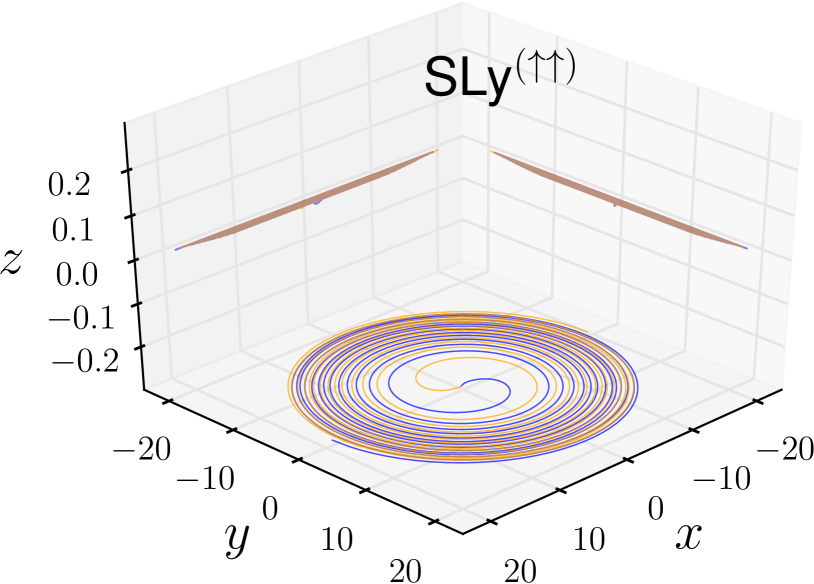
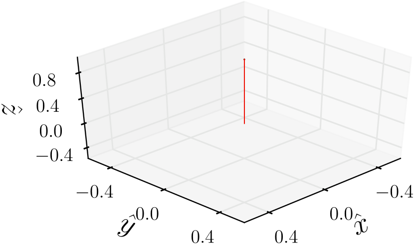
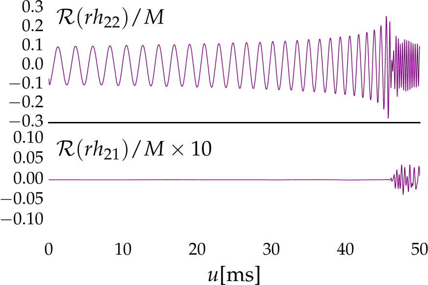
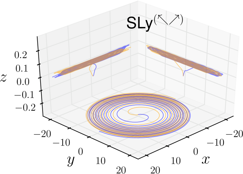
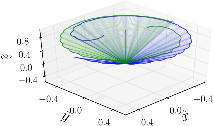
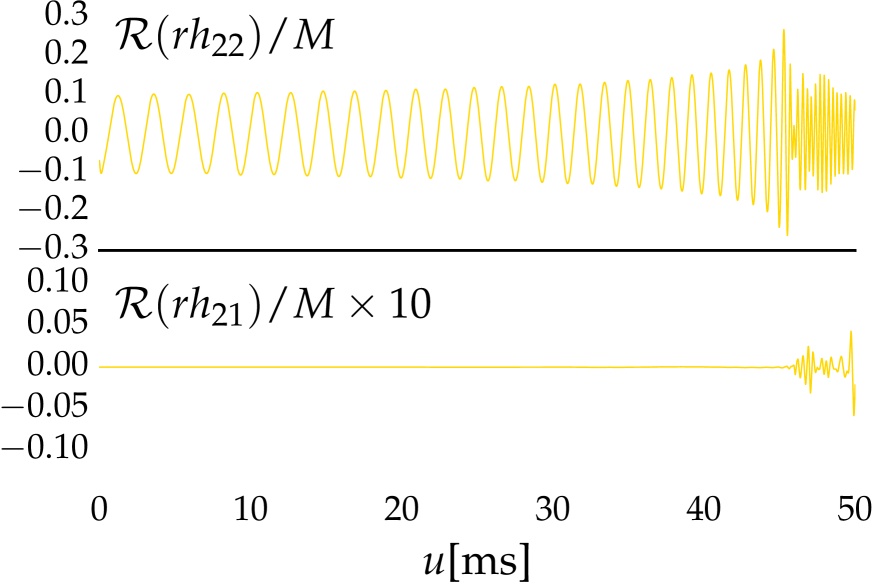
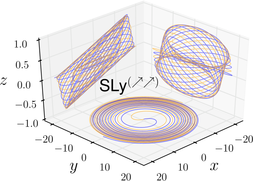
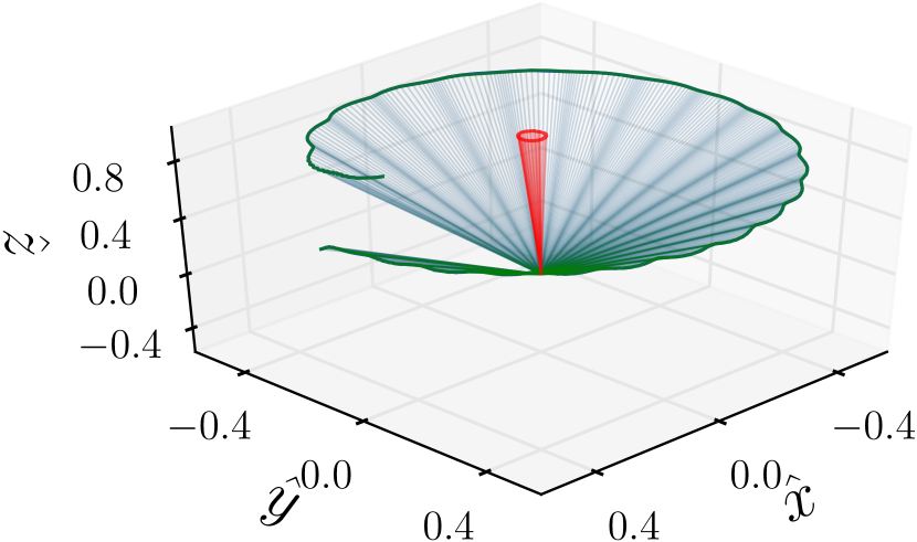
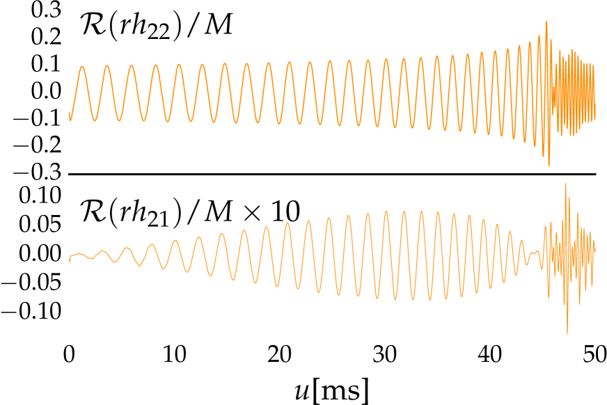
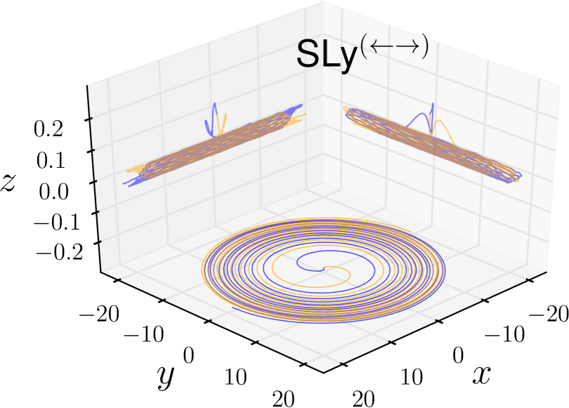
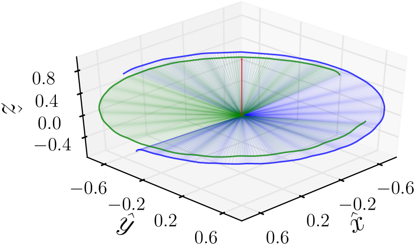
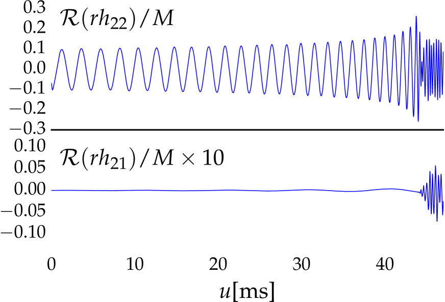
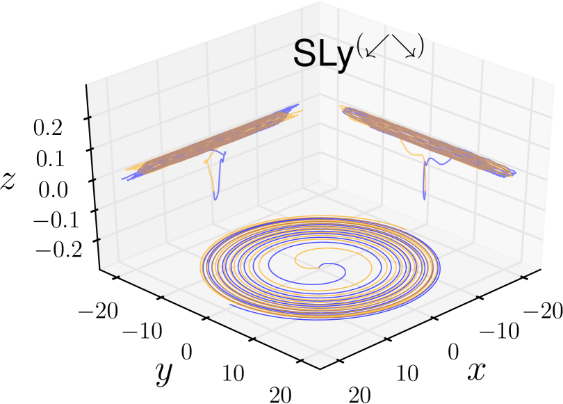
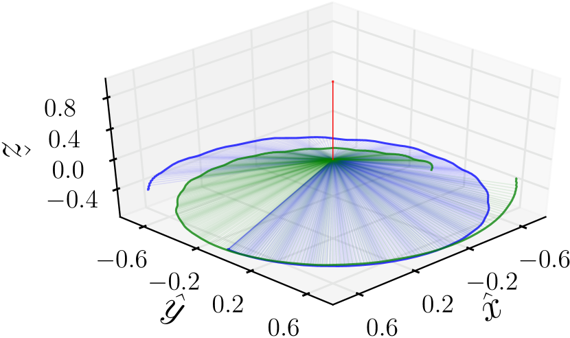
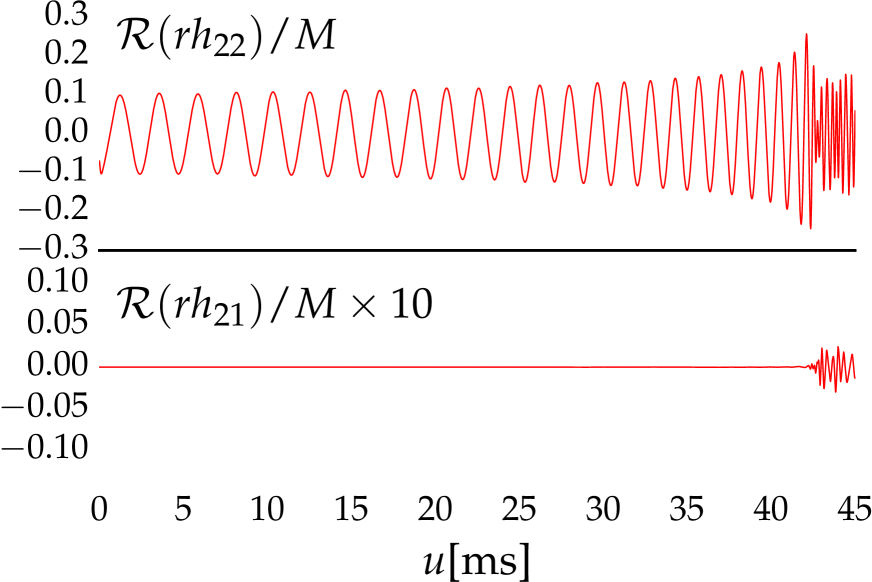
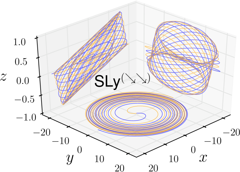
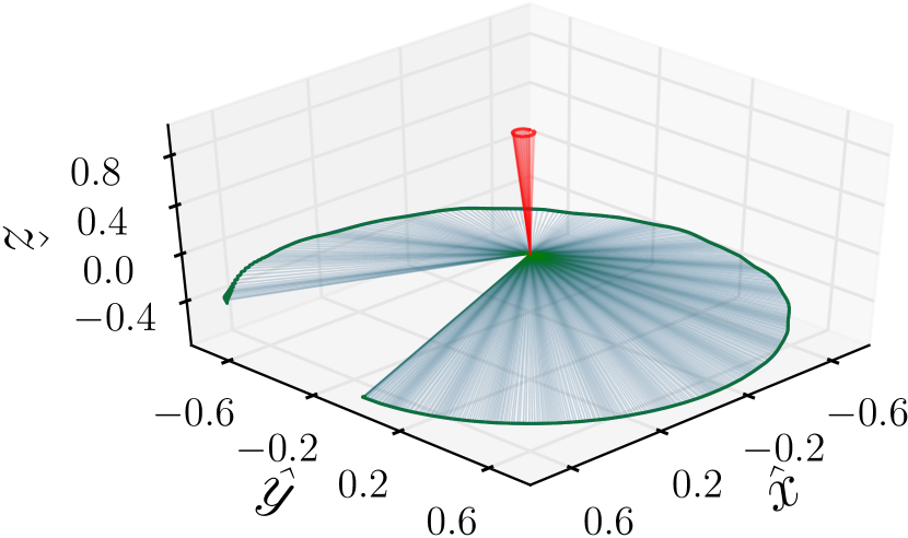
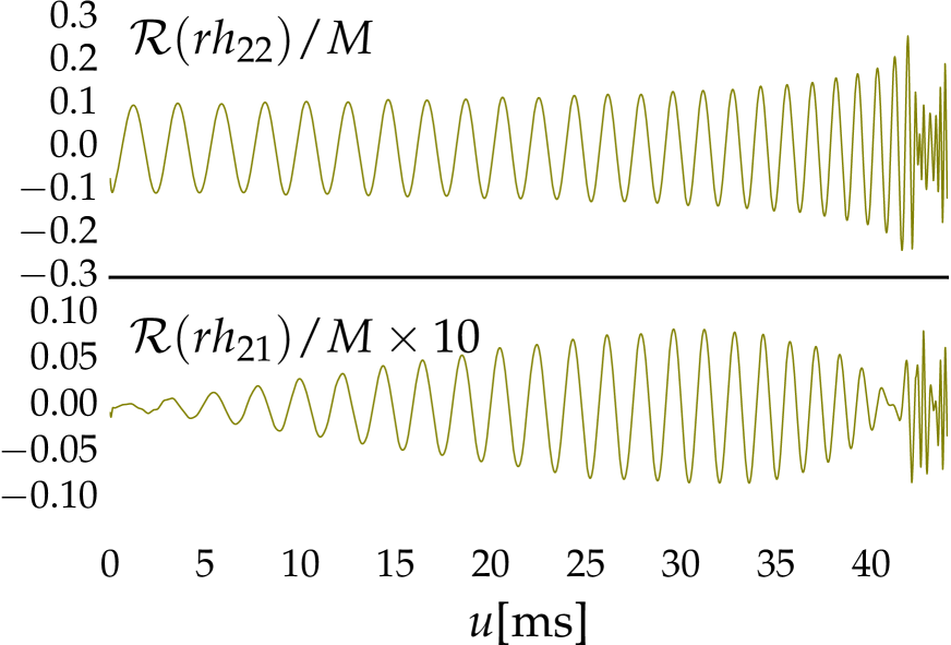
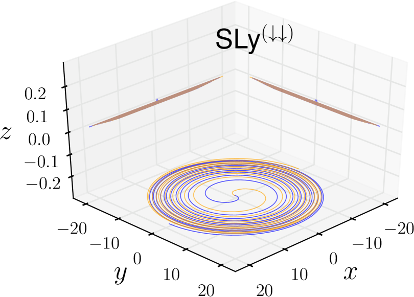
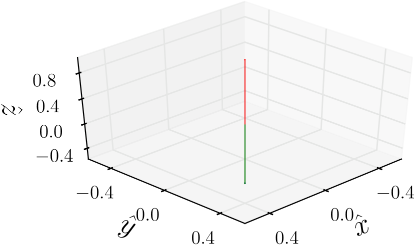
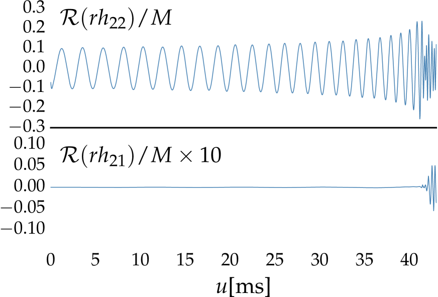
Figure 1: Orbital dynamics and GW emission for all simulations. Column 1 shows the coordinate tracks of each NS in the binary. Column 2 shows the corresponding precession cones. The spin evolution of the individual stars (blue and green), and the orbital angular momentum of the system (red) are shown here. Column 3 shows the (2,2)- and (2,1)-modes of the GW strain $rh$.

III Dynamics

III.1 Qualitative discussion

We start our investigation with a qualitative discussion about all considered systems. For this purpose, we present in Fig. 1 the tracks of the stars (left panels), the precession cones of the individual spins and the orbital angular momentum (middle panels), and the (2,2)- and (2,1)-modes of the GW signal (right panels). The individual rows refer to the different configurations.

Precession effects for SLy^(↗↗) and SLy^(↘↘) are largest due to the misaligned initial spins, which leads to a clearly visible motion of the binaries along the $z-$axis. In addition, the precession cone of the orbital angular momentum has the largest opening angle which confirms our observation that these systems undergo a precessing motion. Moreover, a clear modulation in GW amplitude due to precession can be seen in the (2,1)-mode of the GW signal.

Other configurations, such as SLy^(←→) have clearly different dynamics. Even though the initial spins for this simulation are misaligned, no characteristic precession effect is visible for the orbital angular momentum. As the spins lie in the orbital plane and are opposite and of equal magnitude, any $z-$motion of the stars is in the same direction. This results in a “bobbing” motion of the orbital plane (rather than the “wobbling” motion that is typical for precession). These findings are supported by the corresponding precession cone, which shows no precession of the orbital angular momentum. Furthermore, no precession effects are present in the (2,1)-mode of the GW signal due to the symmetry of this system. However, we find clearly that the individual spins are precessing; cf. blue and green lines in the middle panels.

Similar symmetry arguments can be used to explain why the other symmetrically misaligned simulations show “bobbing” motion in the $z$-direction, but no precession of the orbital plane like the SLy^(↗↗) and the SLy^(↘↘) cases.

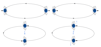
Figure 2: A schematic of the Lense-Thirring effect in a binary system. Left column: A system with symmetrically misaligned-spins of the NSs A and B with respect to the orbital angular momentum direction. Right column: A system with asymmetrically misaligned-spins of the NSs A and B.

Interestingly, the motion of the orbital plane, “wobbling” or “bobbing” for the spin misaligned systems can be explained by considering the general relativistic frame-dragging effect or specifically the Lense-Thirring (LT) effect (Morsink and Stella, 1999). Due to this effect, a rotating mass in general relativity influences the motion of objects in its vicinity i.e., the rotating mass “drags along” spacetime in its vicinity. In Fig. 2 we show a schematic of the frame dragging due to the NS spins. Top row panels show the initial configurations for setups with symmetrically misaligned-spin (left column) and with asymmetrically misaligned-spin (right column) for the NSs A and B. The blue circles represent the two NSs, the black arrows show their spin directions and the dragging of the spacetime is depicted as the circular rings around the NSs. In the top row panel scenario, the stars will feel no LT effect i.e., the dragging due to each other’s spin rotations. The spin orientation of the stars changes very slowly, so that a quarter of an orbit later they will still be pointed in essentially the same direction. This scenario is depicted in the bottom row panels. This time for the symmetrically misaligned system, star B will feel the LT effect due to A in the direction that points into the orbital plane. Since the spin of star B is pointed in the opposite direction, the LT effect on star A will be in the same direction as on star B i.e., into the orbital plane as shown in the bottom left panel. The net result will now push the entire orbital plane in this direction, which is perpendicular to the orbital plane. Half an orbit later, the effect will be in the opposite direction; the resulting motion is an oscillation of the orbital plane in the perpendicular direction i.e., a “bobbing” motion. Similarly, for the asymmetrically misaligned-spin system (right column); stars A and B will be pushed in directions opposite to one another. This results in a zero net force on the orbital plane as shown in the bottom right panel and a nonzero torque that tilts the orbital plane, which over time causes the “wobbling” motion. Therefore, the misaligned-spins of the NSs either produces a torque or a net force on the orbital plane giving rise to either “wobbling” or “bobbing” motions respectively. Additionally, two important observations can be made based on Fig. 1.

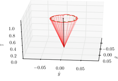
Figure 3: Precession cone for the SLy^(↗↗) configuration for the orbital angular momentum (red). Additionally, as green dashed line we show also the precession cones for $(\hat{L}_{x},\hat{L}_{y},\hat{L}_{z})$ for the SLy^(↘↘) configuration. The opening angles for both the configurations are almost identical, due to the symmetry of the systems.

First, for the SLy^(↑↑) and SLy^(↓↓) configurations there is no precession as their initial spins are (anti-) aligned with the orbital angular momentum. Moreover, the orbital hang-up (speed-up) effect (Campanelli et al., 2006; Bernuzzi et al., 2014), i.e., the fact that spin-aligned systems merge later and vice versa, is clearly visible in the GW signal with respect to the peak time in the amplitude at the merger. This effect also holds for the misaligned systems that have an effective (anti-) aligned spin components with respect to the orbital angular momentum of the system. The exact merger times can be found in Tab. 3 for the R3 setups. Second, apart from precession, the spin misaligned systems also show nutation, i.e., small oscillations in the precession cones for the individual spins (blue and green) as seen in column 2 of Fig. 1. The nutation happens on a much shorter timescale than the precession motion. These nutation cycles are clearly visible for the individual spins for the SLy^(↖↗) and SLy^(↗↗) cases but are also present for the SLy^(↙↘) and SLy^(↘↘) cases. We also show a comparison of the precession cones of the orbital angular momentum for SLy^(↗↗) and SLy^(↘↘) in Fig. 3.

III.2 Energetics

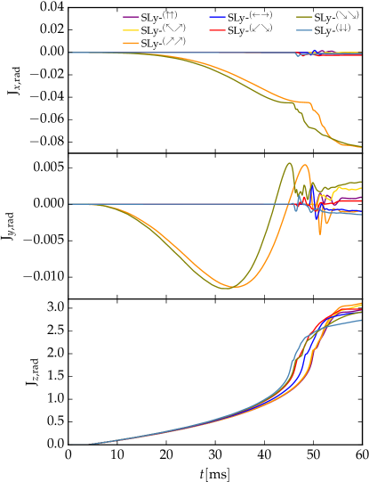
Figure 4: Radiated angular momentum ($\vec{\bf{J}}_{\rm rad}$) in GWs computed using the relations given in Appendix A. For symmetrically misaligned configurations the angular momentum is only radiated in the $z-$component and the $x,y-$components remain identically zero during the inspiral. Whereas for the asymmetrically misaligned systems there is radiation in all the components.

We study the conservative dynamics for all the configurations presented in this article by computing the reduced binding energy,

$$E_{b}=\frac{M_{\rm ADM}(t_{0})-E_{\rm rad}-M}{\nu\ M},$$ (3)

and the specific orbital angular momentum,

$$\ell=\frac{|{\vec{\bf{J}}_{\rm ADM}}(t_{0})-{\vec{\bf{S}}_{A}}(t_{0})-{\vec{\bf{S}}_{B}}(t_{0})-\vec{\bf{J}}_{\rm rad}|}{\nu\ M^{2}}.$$ (4)

Here $\nu:=M^{A}M^{B}/M^{2}$ is the symmetric mass ratio, $E_{\rm rad},\vec{\bf{J}}_{\rm rad}$ are the emitted energy and angular momentum in the radiated GWs, and $M_{\rm ADM},\vec{\bf{J}}_{\rm ADM}$ denote the ADM mass and angular momentum at the beginning of the simulation (i.e. at $t=t_{0}$), ${\vec{\bf{S}}_{A}}(t_{0})$ and ${\vec{\bf{S}}_{B}}(t_{0})$ are estimated from the initial data (Tab. 1), and ${\vec{\bf{S}}}_{A,B}=(M^{A,B})^{2}\chi^{A,B}\hat{\chi}^{A,B}$. In Appendix A, we present a few details about the postprocessing step for the computation of the radiated energy and angular momentum in GWs extracted in numerical relativity simulations employing the BAM code. In Fig. 4, we show the computed angular momentum for all the simulated configurations. One finds that for the symmetrically misaligned configurations (SLy^(←→), SLy^(↖↗), SLy^(↙↘)) the angular momentum is radiated only in the $z-$component whereas the $x,y-$components remain identically zero during the inspiral. For the asymmetrically misaligned systems (SLy^(↗↗)and SLy^(↘↘)) there is radiation in the other components as well.

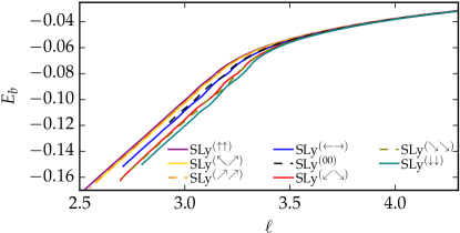
Figure 5: Reduced binding energy $E_{b}$ as a function of the specific orbital angular momentum $\ell$ for all configurations considered in the article. Additionally, we also include the curve for an irrotational case SLy⁽⁰⁰⁾ taken from the CoRe Database (ID:-BAM:0095:R02) for comparison. As expected, the irrotational curve matches nicely to the SLy^(←→) case.

In Fig. 5 we show the $E$-$\ell$ curve for all the configurations for the highest resolution (R4), cf. Tab. 2. For comparison we also show the curve for an irrotational configuration SLy⁽⁰⁰⁾ (‘black line’) with the same masses and EOS. The irrotational setup corresponds to “BAM:0095:R02” from the CoRe database CoR ; Dietrich et al. (2018c). For the early inspiral part of the dynamics (large $E$ and $\ell$), we find that the $E$-$\ell$ curves are very similar for all setups, which is caused by the fact that the main contribution, the point-mass contribution, is identical for all systems.

During the late inspiral part, when the stars come close to each other, due to the emission of energy and angular momentum, a clear difference is present as seen in Fig. 5. Throughout the simulation, the $E$-$\ell$ curve for the irrotational configuration SLy⁽⁰⁰⁾ and the effectively zero-spin configuration ($\chi_{\rm eff}=0$) SLy^(←→) clearly demarcate the effectively aligned spin and the effectively antialigned spin configurations. In general, aligned spin configurations are less bound while the antialigned spin configurations are more bound than the corresponding irrotational setup, cf. Fig. 6 top panel.

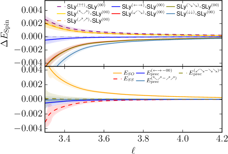
Figure 6: Top panel: Estimate of the spin orientation effects on the conservative dynamics by taking the difference between all the configurations and the SLy⁽⁰⁰⁾(irrotational case taken from CoRe Database) configuration. The shaded region marks the difference in results obtained with a lower resolution and takes into account the uncertainty of the initial data. Bottom panel: Spin and orbital contributions to the binding energy estimated following the discussion in the text.

To better disentangle the different contributions to the total binding energy due to the spin Bernuzzi et al. (2014); Dietrich et al. (2017a), we assume that it consists of a nonspinning contribution including tidal effects $E_{0}$, a spin-orbit $E_{\text{SO}}$ contribution, and a spin-spin contribution $E_{\text{SS}}$,

$$E_{b}=E_{0}+E_{\text{SO}}+E_{\text{SS}}+\mathcal{O}(S^{3}).$$ (5)

In general, the spin-orbit (SO) interaction is at leading order $\propto\vec{\bf L}\cdot\vec{\bf S}_{i}/r^{3}$, see (Kidder et al., 1993). The $\text{SO}-$interaction term is either repulsive or attractive, i.e., positive or negative, according to the sign of $\sum_{i=1}^{2}\vec{\bf L}\cdot\vec{\bf S}_{i}$. The spin-spin term includes the self-spin term (of the form $\vec{\bf S}_{i}\cdot\vec{\bf S}_{i}$) and an interaction term (of the form $\vec{\bf S}_{i}\cdot\vec{\bf S}_{j}\ (i\neq j)$) between the two spins. The spin-spin interaction term in particular is $\propto[3(\vec{\bf n}\cdot{\vec{\bf S}}_{1})(\vec{\bf n}\cdot{\vec{\bf S}}_{2})-({\vec{\bf S}}_{1}\cdot{\vec{\bf S}}_{2})]/r^{3}$ (with $\vec{\mathbf{n}}$ denoting the unit vector pointing from one star to the other and $r$ being the distance between the stars), see e.g. (Kidder et al., 1993). Note that the first term in the interaction term is zero for the (anti-) aligned configurations and the remaining term $\propto-({\vec{\bf S}}_{1}\cdot{\vec{\bf S}}_{2})$ does not change sign if both spins flip. We compute the spin-orbit term $E_{\text{SO}}$ as

$$E_{\text{SO}}=\frac{E_{b}[{\rm SLy}^{(\uparrow\uparrow)}]-E_{b}[{\rm SLy}^{(\downarrow\downarrow)}]}{2},$$ (6)

and estimate the complete spin-spin term, i.e., including the interaction term and the self-spin term as,

$$E_{\text{SS}}=\frac{E_{b}[{\rm SLy}^{(\uparrow\uparrow)}]+E_{b}[{\rm SLy}^{(\downarrow\downarrow)}]}{2}-E_{b}[{\rm SLy}^{(00)}].$$ (7)

The bottom panel in Fig. 6 shows these contributions to the binding energy. We find that compared to the SO-interaction, the spin-spin term is almost negligible during most of the inspiral and mostly within the uncertainty of our data . The SO-contribution is the dominant contribution to the binding energy in our comparison, while in the very late inspiral tidal effects can dominate (Bernuzzi et al., 2014). Intuitively, this is understandable based on the differences in the PN order of the SO (1.5PN), spin-spin (2PN), and tidal effects (5PN).

To get a better understanding of potential precession effects, we also compute

$$E_{\rm prec}^{(\nwarrow\nearrow-\nearrow\nearrow)} =E_{b}[{\rm SLy}^{(\nwarrow\nearrow)}]-E_{b}[{\rm SLy}^{(\nearrow\nearrow)}],$$ (8)

$$E_{\rm prec}^{(\swarrow\searrow-\searrow\searrow)} =E_{b}[{\rm SLy}^{(\swarrow\searrow)}]-E_{b}[{\rm SLy}^{(\searrow\searrow)}],$$ (9)

$$E_{\rm prec}^{(\leftarrow\rightarrow-00)} =E_{b}[{\rm SLy}^{(\leftarrow\rightarrow)}]-E_{b}[{\rm SLy}^{(00)}],$$ (10)

and show the results in the bottom panel of Fig. 6. We find that the configurations (SLy^(↖↗) & SLy^(↗↗)) and (SLy^(↙↘) & SLy^(↘↘)) are almost identical with respect to their binding energy contribution. Also the difference between the irrotational case and SLy^(←→)is not clearly resolved in our simulations. The reasons for this could be due to (i) the fact that the spins are rather small to show any distinguishable effect and (ii) that even the highest resolution employed in the simulations presented in this article falls short in resolving the differences between those configurations. Therefore, even though the tracks and the precession cones, cf. Fig. 1, show clear imprints of precession, the energetics does not shed light on the differences, at least among the abovementioned pairs.

III.3 Merger remnant

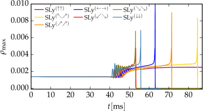
Figure 7: Maximum of $\rho$ vs. coordinate time $t$. The cases that form a black hole (BH) after the merger show a sharp change in the density where the density drops to zero for such cases, because matter is removed inside the BH. Note that we report the merger remnant properties for the R3 resolution setups as the simulations could be evolved for longer times owing to the reduced computational costs.

Table 3: Properties of the merger remnant. The columns represent: (i) the name of the configuration (ii) the merger time in $M_{\odot}$ and in ms (iii) the lifetime, $\tau$, of the HMNS formed during our simulation, given in $M_{\odot}$ and in ms; (iv) the final mass of the BH, $M_{\text{BH}}$, if the HMNS collapsed during our simulation; the dimensionless spin of the final BH, $\chi_{\text{BH}}$ and the mass of the disk surrounding the BH, $M_{\text{disk}}$. The different physical quantities are computed for resolution R3. Note that the case SLy^(↑↑) did not undergo collapse to a BH during our simulation time and therefore the corresponding quantities are marked as “$-$”.

Name	$t_{\rm merge}$		$\tau$		$M_{\text{BH}}$	$\chi_{\text{BH}}$	$M_{\text{disk}}$
	$[M_{\odot}]$	$[\rm ms]$	$[M_{\odot}]$	$[\rm ms]$	$[M_{\odot}]$		$[M_{\odot}]$
SLy(↑↑)	9981	49.16	$>12532$	$>61.72$	$-$	$-$	$-$
SLy(↖↗)	9923	48.88	7074	34.84	2.37	0.57	0.215
SLy(↗↗)	9919	48.86	4421	21.78	2.42	0.62	0.165
SLy(←→)	9622	47.39	3062	15.08	2.40	0.59	0.167
SLy(↙↘)	9275	45.68	1394	6.87	2.45	0.62	0.113
SLy(↘↘)	9230	45.46	1471	7.25	2.45	0.62	0.123
SLy(↓↓)	9064	44.64	2156	10.62	2.41	0.57	0.135

In Tab. 3 we show the properties of the remnants obtained from the R3 resolution, since due to the high computational costs the R4 resolutions are not evolved for a long time after the merger. Until the end of our simulations all the runs except SLy^(↑↑) collapsed into a black hole, see Fig. 7 where the maximum of the density is shown as an indicator of the BH formation. In general, the lifetime of the HMNS decreases when we go from the aligned spin setups to the antialigned spin setups, an indicator that the presence of spins influences the angular momentum support counteracting the gravitational collapse, see also Kastaun and Galeazzi (2015); Dietrich et al. (2017a). Aligned spin configurations, and SLy^(↑↑) in particular, have additional angular momentum support which allows a longer HMNS lifetime. Similar behavior was also found in Dietrich et al. (2017a). While we find that aligned spin configurations lead to more massive disks and less massive BHs, cf. Kastaun et al. (2013); Bernuzzi et al. (2014), which is directly caused by the delayed BH formation which allows for better angular momentum and matter redistribution into the outer layer of the remnant, we do not find any trend in the remnant spins. This can be attributed to the fact that more refinement is required to resolve the BH formed after the merger and therefore the inferred properties can incur some errors.

IV Ejecta and Kick estimates

IV.1 Ejecta

During our simulations, unbound matter is mainly ejected in the very late inspiral from the tidal tail ejection mechanism or from shock heating during the collision of the cores of the NSs. In general, our simulations are too short to estimate properly disk wind ejecta.

We compute the amount of ejected matter as shown for the R3 and R4 resolution simulations in Tab. 4. In general, we mark matter as unbound if it fulfills

$$u_{t}<-1\quad\text{and}\quad v^{i}x_{i}>0\ ,$$ (11)

where $u_{t}=-W(\alpha-\beta_{i}v^{i})$ is the time component of the fluid 4-velocity (with a lowered index), $\alpha$ is the lapse, $\beta^{i}$ is the shift vector, $W$ is the Lorentz factor, and $x^{i}=(x,y,z)$. For Eq. (11) we assume that the fluid elements follow geodesics and require that the orbit is unbound and has an outward pointing velocity, cf. also East and Pretorius (2012).

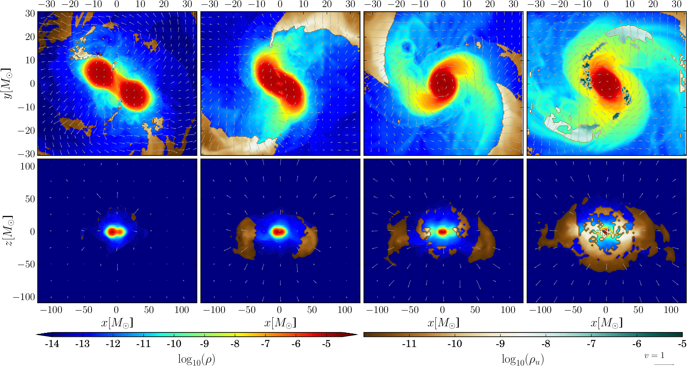
Figure 8: 2D-plots for the SLy^(↙↘) configuration showing the density and velocity field at different times close to the merger, with the unbound material shown in the brown to green color scale, while the bound material is shown in a blue to red color scale. Top row: plots show the $xy-$plane covering a distance of $\sim 88$ km in each direction; Bottom row: plots show the $xz-$plane, where each direction is covering a distance of $\sim 293$ km. Columns one to three: Time snapshots when the surfaces of the stars touch until the cores of the NSs finally merged. Fourth column: Postmerger phase when a hypermassive NS has been formed. Interestingly, we see that in the final phase of the merger unbound matter is ejected asymmetrically due to the “bobbing” motion that this system undergoes. Such an asymmetrical matter ejection is capable of imparting a kick velocity to the merger remnant.

Bound and unbound matter along with their velocity profile is shown for the SLy^(↙↘) case in Fig. 8. Here, we see that the matter ejection does not happen until the NSs collide (column one). After that (column two), unbound matter characterized with a density $\sim\mathcal{O}(10^{-9})-\mathcal{O}(10^{-8})$ ($\sim\mathcal{O}(10^{8})-\mathcal{O}(10^{9})$ g cm^-3) can be seen coming out from the tidal tail mostly in the orbital plane (note that this case shows a “bobbing” motion of the orbital plane, see Fig. 1). These ejecta quickly expand into the volume surrounding the system, dropping in density by several orders of magnitude. Once the cores of the NSs have merged (column three) there are also ejecta in the direction normal to the orbital plane due to shock heating. During these last phases in the merger unbound matter characterized with a density $\sim\mathcal{O}(10^{-8})-\mathcal{O}(10^{-6})$ ($\sim\mathcal{O}(10^{9})-\mathcal{O}(10^{11})$ g cm^-3) is ejected. In principle, unlike equal-mass nonprecessing quasicircular BNSs where the matter should be symmetrically ejected, similar setups for precessing BNSs can eject matter asymmetrically due to the “wobbling” or the “bobbing” motion of the system. This asymmetrical ejection of matter would then give rise to electromagnetic counterparts with a more complicated geometry.

From Tab. 4 we see that the amount of unbound matter increases when the spin of the NS is effectively antialigned to the orbital angular momentum. This indicates that the ejecta is dominated via shock heating during the merger of the cores of the two stars, see also Kastaun et al. (2017); Most et al. (2019). Overall, $\sim\mathcal{O}(10^{-3})-\mathcal{O}(10^{-2})\ M_{\odot}$ ($\sim\mathcal{O}(10^{30})-\mathcal{O}(10^{31})$ g) of unbound matter is ejected for the studied configurations. We find the relative error in the estimate of the ejecta mass to be $\sim 2\%-40\%$ between the R3 and R4 resolution setups. No strong effect of precession is found on the ejecta mass within our simulations.

Table 4: Ejecta mass from the volume integral $M_{\text{ej}}^{\mathcal{V}}$ (cf. Chaurasia et al. (2018)) for the R3 and R4 resolution setups.

Name	$M_{\text{ej}}^{\mathcal{V}}[M_{\odot}]$
	R3	R4
SLy(↑↑)	$0.0053$	$0.0043$
SLy(↖↗)	$0.0045$	$0.0062$
SLy(↗↗)	$0.0031$	$0.0054$
SLy(←→)	$0.0111$	$0.0162$
SLy(↙↘)	$0.0192$	$0.0188$
SLy(↘↘)	$0.0210$	$0.0189$
SLy(↓↓)	$0.0275$	$0.0192$

IV.2 Kick estimates

In addition to the kicks obtained from the asymmetrical matter ejection mechanism briefly described in the previous subsection, the anisotropic loss of linear momentum radiated away via the emission of GWs also imparts a recoil or kick on the remaining system which then moves relative to its original center-of-mass frame. This effect can be particularly pronounced for the inspiral and merger of two compact objects, for BBH cases; see e.g. Gonzalez et al. (2007); Brügmann et al. (2008); González et al. (2007).

In Fig. 9 we show the estimates for the kick speed computed from the ejecta and from the emission of GWs for the R4 resolution setups. The kick estimates from the ejecta are computed from the conservation of linear momentum for the unbound matter whereas the estimates from GWs are computed using the linear momentum conservation for the GWs using the relations given in Appendix A. As expected, aligned (and antialigned) systems considered in this article being symmetrical, the kicks imparted from the GWs are negligible ($<5$ km s^-1). Furthermore, for the symmetrically misaligned configurations considered that undergo “bobbing” motion, we find the kick speeds to be in the range $\sim 15-50$ km s^-1 and is mostly contributed from the motion of the orbital plane giving rise to asymmetrical matter ejection. For the asymmetrically misaligned configurations, for example in the bottom panel of Fig. 9, we find that the kicks are again mostly contributed from the matter ejection, e.g., $\sim 40$ km s^-1 for the SLy^(↘↘) case. In general, we obtain larger recoils for the effectively antialigned configurations than for the aligned spin configurations, but do not see a noticeable difference between the “wobbling” and “bobbing” setups. The kicks from the R3 setups for the configurations shown in Fig. 9 are estimated to be $<10$ km s^-1 for the aligned case and $\sim 52$ km s^-1 for the asymmetrically misaligned case.

Overall, for all simulated cases the kick imparted from the GW emission contributes less than the recoil from unbound matter ejection. This might be due to the “smaller” spins of neutron stars in comparison to BHs, for the latter much larger kicks of $\sim\mathcal{O}(10^{3})$ km s^-1, e.g., Gonzalez et al. (2007), can be obtained due to the anisotropic emission of GWs.

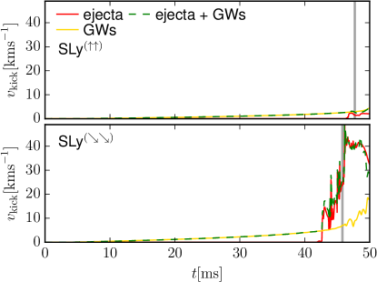
Figure 9: Top panel: Kick estimates for the SLy^(↑↑) case. The aligned/antialigned cases do not show the “bobbing” or the “wobbling” motion of the orbital plane. Bottom panel: Kick estimates for the SLy^(↘↘) case that shows the “wobbling” motion of the orbital plane. The kicks are estimated using the recoil from the ejecta and the GWs and are shown for the R4 setup. The merger time, corresponding to the peak in the (2,2)-mode of GW strain is shown as ‘gray’ line.

V Gravitational Waves

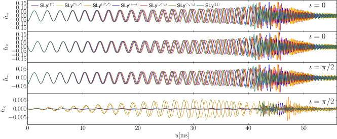
Figure 10: Gravitational wave strains $h_{+}$ (first and third panels) and $h_{\times}$ (second and fourth panels) for the inclinations $\iota=0$ (face on, top panels) and $\iota=\pi/2$ (edge on, bottom panels).

V.1 Qualitative discussion

The individual modes with respect to the $-2$-spin-weighted spherical harmonics of the curvature and the metric scalars are obtained following Sec. VIA of Chaurasia et al. (2018) and references therein. Additionally, in this article we compute the GW strain $h$ by summing all modes up to $\ell\leq 4$. All waveforms are shown against the retarded time

$$u=t-r_{*}=t-t_{\rm extr.}-2M\ln(r_{\rm extr.}/2M-1).$$ (12)

Figure 10 shows the $h_{+}$ and $h_{\times}$ polarizations of the GW strain,

$$h_{+}-ih_{\times}=\sum_{\ell=2}^{4}\sum_{m=-\ell}^{\ell}h_{\ell m}\ ^{-2}Y_{\ell m}(\theta=\iota,\phi=0),$$ (13)

for two inclinations: face on $\iota=0$ (two top panels) and edge on $\iota=\pi/2$ (two bottom panels). Similar inferences can be made as those from column-three of Fig. 1. As expected, we see that for $\iota=0$ (face on) any imprint of precession is hardly visible and that the $h_{+}$ or $h_{\times}-$polarizations have the same magnitude. The GW strain is, as discussed before, mainly determined by the effective spin $\chi_{\rm eff}$ and the spin-orbit-contribution.

Precession effects with more than one precession cycle are visible in $h_{\times}$ for $\iota=\pi/2$ (edge on) for SLy^(↗↗) & SLy^(↘↘). For these cases, the amplitude of $h_{\times}(\iota=\pi/2)$ is about $10$ times smaller than for $h_{+}(\iota=\pi/2)$ and 30 times smaller than $h_{\times}(\iota=0)$ or $h_{+}(\iota=0)$. For the nonprecessing cases, the signal amplitude of $h_{\times}$ is even smaller as already seen in Fig. 1 for the (2,1)-mode of the GW strain.

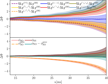
Figure 11: Top panel: Phase differences for all spinning configurations with respect to the irrotational case for the (2,2)-mode of the GW strain. The errors represented by the shaded regions are estimated by computing the phase differences for different resolutions. Note again that the irrotational case data used, namely R3 (0.118 $M_{\odot}$) and R4 (0.078 $M_{\odot}$) resolutions, are not of exactly the same resolution as the other configurations simulated and therefore the error estimates should be taken as conservative estimates. Bottom panel: Estimate of spin-orbit and spin-spin contribution to the phase from the aligned/antialigned configurations as described in the text.

V.2 Phasing analysis

In this subsection we discuss briefly the phase evolution for the different configurations by considering the phase differences between them for the (2,2)-mode of the GW strain $h$. Note that the irrotational case SLy⁽⁰⁰⁾ is aligned with SLy^(←→) configuration in the interval $\hat{\omega}:=M\omega_{22}\in[0.040,0.048]$ for the analysis purpose.

In Fig. 11, the phase differences are shown for the spinning configurations with respect to the nonspinning configuration (top panel). It is clearly visible that the effectively antialigned systems undergo accelerated inspiral and the aligned systems undergo decelerated inspiral. These phase differences are again dominated by the leading-order spin-orbit coupling. The irrotational case and the SLy^(←→) case are almost indistinguishable with negligible difference with respect to phase difference.

To isolate the effect of different contributions to the phase evolution we consider, similar to the binding energy discussion, different linear combinations of the numerical simulations, but we emphasize that this analysis is not gauge invariant, i.e., it only allows for a qualitative interpretation. In particular, we consider for the spin-orbit contribution,

$$\phi_{\text{SO}}=\frac{\phi[\text{SLy}^{(\uparrow\uparrow)}]-\phi[\text{SLy}^{(\downarrow\downarrow)}]}{2},$$ (14)

and for the spin-spin contribution,

$$\phi_{\text{SS}}=\frac{\phi[\text{SLy}^{(\uparrow\uparrow)}]+\phi[\text{SLy}^{(\downarrow\downarrow)}]}{2}-\phi[\text{SLy}^{(00)}].$$ (15)

To estimate the effect of precession, we also compute

$$\phi^{\text{prec}}_{\text{SO}}=\sqrt{2}\frac{\phi[\text{SLy}^{(\nwarrow\nearrow)}]-\phi[\text{SLy}^{(\swarrow\searrow)}]}{2},$$ (16)

where the factor $\sqrt{2}$ is introduced to compensate for the fact that the effective spin of the precessing configurations is smaller than for the spin-aligned setups.

Figure 11 (bottom panel) shows these contributions. Considering the spin-orbit contribution, we find almost no difference between the spin-aligned and the precessing setups, in fact, the difference between both contributions can not be resolved with our simulations; cf. solid green line in the bottom panel of Fig. 11 and the discussion on waveform accuracy in Appendix B. Overall, the spin-orbit contribution dominates so that the spin-spin effect is about a factor 3 smaller. Considering our error estimate, we find that for the last few orbits, the spin-spin contribution is reliably measured as nonzero.

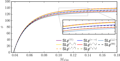
Figure 12: $\phi(\hat{\omega})$ accumulated in $\hat{\omega}\in$ [0.038,0.18] for all the configurations considered for the R4 resolution.

In order for a more quantitative analysis, we analyze the phasing of the waves by considering $\phi(\hat{\omega})$. We fit $\phi(\hat{\omega})$ with a function,

$$f(\hat{\omega})=\frac{\sum_{n=0}^{4}a_{n}\hat{\omega}^{n}}{\sum_{n=0}^{4}b_{n}\hat{\omega}^{n}},$$ (17)

eliminating this way the residual eccentricity oscillations in the NR data. We then align the curves to start at the same frequency $\hat{\omega}=0.038$. The phase comparison is restricted to the frequency interval $\hat{\omega}=[0.038,0.18]$ which corresponds to physical GW frequencies $\sim$ 455 - 2153 Hz. Figure 12 summarizes our results of the comparison of the accumulated phase difference in the mentioned frequency interval. Overall, we again find the dominant spin-orbit contribution to give rise to the different accumulated phases at a particular frequency for the different configurations. Precession effects are again hardly visible. One can also see in the inset plot in Fig. 12 that the SLy⁽⁰⁰⁾ and SLy^(←→) are indistinguishable considering the accumulated phases for the dominant GW mode.

V.3 Comparison with precessing tidal GW approximant

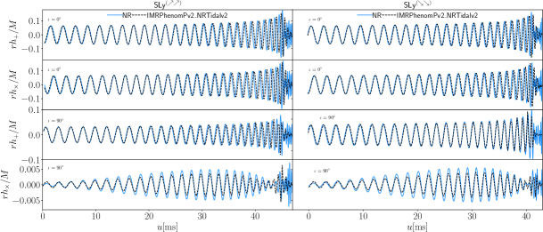
Figure 13: Rescaled GW strains for the precessing systems SLy^(↗↗) (left panel) and SLy^(↘↘) (right panel) (blue, solid curves) for the R4 resolution compared with the IMRPhenomPv2_NRTidalv2 model (black, dashed curve). Results for $h_{+}$ are shown in first and third panel and for $h_{\times}$ are shown in the second and fourth panels for the inclinations $\iota=0$ (face on) in top panels and $\iota=\pi/2$ (edge on) in bottom panels. Note that we find small differences in the amplitudes (as visible in the $h_{\times}$-panels for the $\iota=\pi/2$ case) indicating the importance of future GW waveform model development.

One important advantage of full numerical relativity simulations is their potential usage for the validation of existing waveform approximants. Until now, the only two existing precessing, tidal waveform models are IMRPhenomPv2_NRTidal Dietrich et al. (2019a) and IMRPhenomPv2_NRTidalv2 Dietrich et al. (2019b). We focus on the comparison against IMRPhenomPv2_NRTidalv2 in the following.

IMRPhenomPv2_NRTidalv2 is a phenomenological, frequency domain, tidal-precessing model that augments the aligned-spin binary black hole model, IMRPhenomD Khan et al. (2016); Husa et al. (2016) with the NRTidalv2 Dietrich et al. (2019b) tidal description. In addition, it incorporates all the relevant EOS dependent spin-spin effects and cubic-in-spin effects at 2PN, 3PN, and 3.5PN; and in addition a tidal amplitude correction that is added to the binary black hole amplitude. To ensure that the system can describe precession effects, the aligned-spin waveform is modified by following the framework outlined in Schmidt et al. (2012, 2015).

We align the IMRPhenomPv2_NRTidalv2 waveforms with the numerical relativity waveforms by varying the time translations and phase shifts. To obtain the phase and time shift, we minimize the phase difference between the waveforms in the time interval $u\in[5,18]$ ms which corresponds to roughly $8$ GW cycles. In addition, we also vary slightly the “reference frequency” at which the orientation of individual spins are fixed for the construction of the precessing IMRPhenomPv2_NRTidalv2 model. While the numerical relativity simulations have an initial frequency of $\sim 407~{}\rm Hz$, we use $410~{}\rm Hz$ instead to account for the initial transition caused by gauge changes in the simulation.

The comparison among the precessing systems SLy^(↗↗) (left panel) and SLy^(↘↘) (right panel) and the IMRPhenomPv2_NRTidalv2 model is shown in Fig. 13 for two inclination angles, $\iota=0$ (face on) in top panels and $\iota=\pi/2$ (edge on) in bottom panels. We find that the model is in good agreement with the NR waveforms and also captures precessing motion, i.e., the modulation of the GW strain, adequately as shown in bottom panels. The phase difference between the numerical relativity waveforms and IMRPhenomPv2_NRTidalv2 is about 1 radian for an inclination of $\iota=0$ and about 1.2 radian for $\iota=\pi/2$, just before the merger.

V.4 Postmerger

To understand the postmerger evolution of the GW signal we compute the spectrograms as described in Chaurasia et al. (2018). Figure 14 shows the spectrograms for all the configurations under the assumption of $\iota=\pi/2$. In Tab. 5 we report important characteristic frequencies, namely, the merger frequency and the postmerger frequencies $f_{1}$, the dominant $f_{2}$ frequency, and $f_{3}$.

We find that for our chosen EOS and masses the dominant $f_{2}$-peak frequency lies at $\approx 3400$ Hz. In addition to the $f_{2}$-peak frequency other side peaks and frequencies are visible. These peaks are harmonics of the $f_{2}$ frequency and have amplitudes that are typically $2$ to $3$ orders of magnitude smaller . These peaks correspond to emission at about $f_{1}\approx 1800$ Hz and $f_{3}\approx 5600$ Hz, respectively.

We find that the merger frequencies are higher for the aligned spin cases than for the antialigned cases; cf. Dietrich (2016). The postmerger frequencies reported in Tab. 5 are obtained from the individual modes of the GW strain and in some cases were not available possibly due to low signal amplitude or the lifetime of the remnant before BH formation. However, in Fig. 14 where the spectrogram was obtained from $h$ those frequencies are visible albeit with smaller amplitudes relative to the prominent $f_{2}$ frequency. The frequency estimates have typical uncertainties of $\sim 50-100$ Hz.

For comparison, the estimates for the dominant $f_{2}$ frequency using Ref. (Tsang et al., 2019, Eq. (8)) gives a frequency of $\sim 3372$ Hz and the quasiuniversal relation of Ref. (Breschi et al., 2019, Eq. (13)) gives a frequency of $\sim 3435$ Hz. Both relations do not include spin effects and their estimates are below our simulation results, but are generally in agreement if the uncertainties of the quasiuniversal relations and our numerical relativity simulations are taken into account. This is interesting and hints towards the fact that while spin affects the postmerger dynamics, it only has a minor effect on the main postmerger emission frequency as outlined in Bauswein et al. (2016). Other previous simulations clearly showed spin effects Bernuzzi et al. (2014), so that we conclude that more simulations focusing specifically on the postmerger evolution are needed to solve the existing tension.

Table 5: Postmerger properties. The columns give the name of the configuration, the dimensionless merger frequency $M\omega_{\rm mrg}$, the dimensionful merger frequency $f_{\rm mrg}$ (in Hz), and the dominant postmerger frequencies extracted from the $(2,1)$, $(2,2)$, and $(3,3)$ modes of GW strain $h$. We mark “$-$” for cases where the frequencies could not be extracted properly.

Name	$M\omega_{\text{mrg}}$	$f_{\rm mrg}$	$f_{1}$	$f_{2}$	$f_{3}$
		[Hz]	[Hz]	[Hz]	[Hz]
SLy(↑↑)	$0.165$	$1974$	$1845$	$3358$	$5187$
SLy(↖↗)	$0.170$	$2034$	$1794$	$3557$	$5446$
SLy(↗↗)	$0.177$	$2118$	$1826$	$3620$	$5351$
SLy(←→)	$0.150$	$1795$	$-$	$3431$	$5855$
SLy(↙↘)	$0.150$	$1795$	$-$	$3400$	$-$
SLy(↘↘)	$0.143$	$1711$	$1826$	$3463$	$5257$
SLy(↓↓)	$0.140$	$1675$	$-$	$3447$	$5918$

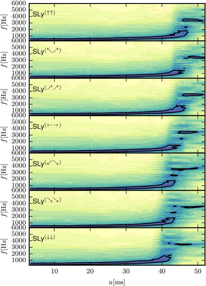
Figure 14: Spectrograms and the corresponding contours for all the configurations computed using the GW strain $h$. An inclination angle of $\iota=\pi/2$ is assumed for all the plots and a logarithmic color scale is used. All individual chunks of the spectrogram have a length of $\sim$ 2 ms and a tapering with a tanh-function is applied before Fourier transforming to minimize oscillations.

VI Summary

In this article we have continued our systematic study of the BNS parameter space where we had previously focused on the effect of the mass ratio Dietrich et al. (2017b), spin Dietrich et al. (2017a), and eccentricity Chaurasia et al. (2018), now, we investigated the influence of the spin orientation. For this purpose, we have studied seven different configurations, from which two setups have aligned/antialigned spins and five setups have misaligned-spins; cf. Tab. 1 for the simulation details. All configurations are simulated for multiple grid resolutions to provide an estimate for the uncertainty of our results; cf. Tab. 2.

In the following, we want to summarize our main findings:

1. Depending on the particular spin configuration, we have systems showing a “bobbing” motion of the orbital plane, i.e., an up- and downward movement of the plane, and systems showing a “wobbling” motion in which the orbital plane precesses. For “wobbling” systems the (2,1)-mode of the GW signal is significantly stronger than for the “bobbing” or aligned-spin setups.

2. Spin-orbit and spin-spin contributions to the binding energy can be extracted from our simulations, but no clear imprint of precession effects is visible in our simulations independent of the spin orientation.

3. Only for the “wobbling” configurations the emitted GWs carry angular momentum that is not parallel to initial orbital angular momentum; cf. Fig. 4.

4. The lifetime of the formed HMNS depends on the effective spin of the system and not on the orientation of the spin, so that systems with positive $\chi_{\rm eff}$ have more angular momentum support at merger and consequently a delayed BH formation in the postmerger stage. In these cases, the disk mass increases while the final BH mass decreases.

5. For the precessing systems, mass can be ejected anisotropically and the final remnant can obtain a kick of $\sim 40\rm km/s$. The anisotropic mass ejection of matter contributes more to the final kick velocity than the anisotropic emission of GWs.

6. Configurations with antialigned spin create a larger ejection of matter compared to spin-aligned systems.

7. The precessing and tidal GW approximant IMRPhenomPv2_NRTidalv2 is capable of describing the inspiral signal and capturing the precessing motion of the studied cases.

8. For the astrophysically motivated cases in which only one star has a non-negligible spin, we expect that there will only be a “wobbling” motion of the orbital plane and no “bobbing” motion. Additionally, if the spin of the individual star is constant, spin-orbit effects will have a smaller impact and the same will be true for the spin-spin terms as there will only be a self-spin term whereas the spin-spin interaction term will vanish. Moreover, we still expect to see orbital hang-up or speed-up effect but with a smaller effect on the orbital dynamics. Other such inferences based on the presented set of simulation results also follow.

Overall, this work has been a first step towards a better understanding of precession effects for BNS systems, but further simulations for unequal-mass systems, unequal spins, and higher spins need to be studied in the near future. To allow the best usage of our simulation data, we will release the waveform signals in the near future as a part of the CoRe database CoR ; Dietrich et al. (2018c).

Appendix A Radiated Energy, Angular Momentum and Linear Momentum Computation

To compute the amount of energy, angular momentum and linear momentum radiated away from the system in the form of gravitational radiation we use the relations as given on pages 313-316 of Alcubierre (2008). The energy is computed from the time integral of

$$\frac{dE}{dt}={\lim_{r\rightarrow\infty}}\ \frac{r^{2}}{16\pi}\ {\sum_{\ell,m}}\ \left\lvert\ {\int^{t}_{-\infty}}A^{\ell,m}\ dt^{\prime}\ \right\rvert{{}^{2}}.$$ (18)

The angular momentum vector is computed from the time integral of

$$\frac{dJ_{x}}{dt}= {-\lim_{r\rightarrow\infty}}\ \frac{ir^{2}}{32\pi}\ {\bf Im}\left\{{\sum_{\ell,m}}{\int^{t}_{-\infty}}{\int^{t^{\prime}}_{-\infty}}A^{\ell,m}\ {dt^{\prime\prime}}\ dt^{\prime}\right.$$

$$\times\left.{\int^{t}_{-\infty}}\left(f_{\ell,m}A^{*\ell,m+1}+f_{\ell,-m}A^{*\ell,m-1}\right)\ dt^{\prime}\right\},$$ (19)

$$\frac{dJ_{y}}{dt}= {-\lim_{r\rightarrow\infty}}\ \frac{r^{2}}{32\pi}\ {\bf Re}\left\{{\sum_{\ell,m}}{\int^{t}_{-\infty}}{\int^{t^{\prime}}_{-\infty}}A^{\ell,m}\ {dt^{\prime\prime}}\ dt^{\prime}\right.$$

$$\times\left.{\int^{t}_{-\infty}}\left(f_{\ell,m}A^{*\ell,m+1}-f_{\ell,-m}A^{*\ell,m-1}\right)\ dt^{\prime}\right\},$$ (20)

$$\frac{dJ_{z}}{dt}= {-\lim_{r\rightarrow\infty}}\ \frac{ir^{2}}{16\pi}\ {\bf Im}\left\{{\sum_{\ell,m}}\ m{\int^{t}_{-\infty}}{\int^{t^{\prime}}_{-\infty}}A^{\ell,m}\ {dt^{\prime\prime}}\ dt^{\prime}\right.$$

$$\times\left.{\int^{t}_{-\infty}}\ A^{*\ell,m}\ dt^{\prime}\right\},$$ (21)

where, $f_{\ell,m}:=\sqrt{(\ell-m)(\ell+m+1)}$ = $\sqrt{\ell(\ell+1)-m(m+1)}$ and ${\bf Im}(a+ib)=ib$ for real $a$ and $b$.

The radiated linear momentum is calculated from the time integral of

$$\frac{dP_{+}}{dt} =\lim_{r\rightarrow\infty}\frac{r^{2}}{8\pi}\sum_{\ell,m}\int^{t}_{-\infty}dt^{\prime}\ A^{\ell,m}$$

$$\times\int^{t}_{-\infty}dt^{\prime}\left(a_{\ell,m}A^{*\ell,m+1}+b_{\ell,-m}A^{*\ell-1,m+1}\right.$$

$$\left.-b_{\ell+1,m+1}A^{*\ell+1,m+1}\right)\ ,$$ (22)

$$\frac{dP_{z}}{dt} =\lim_{r\rightarrow\infty}\frac{r^{2}}{16\pi}\sum_{\ell,m}\int^{t}_{-\infty}dt^{\prime}\ A^{\ell,m}$$

$$\times\int^{t}_{-\infty}dt^{\prime}\left(c_{\ell,m}A^{*\ell,m}+d_{\ell,m}A^{*\ell-1,m}\right.$$

$$\left.+d_{\ell+1,m}A^{*\ell+1,m}\right)\ ,$$ (23)

where $P_{+}=P_{x}+iP_{y}$ and we defined the quantities

$$a_{\ell,m} :=\frac{\sqrt{(\ell-m)(\ell+m+1)}}{\ell(\ell+1)}\ ,$$

$$b_{\ell,m} :=\frac{1}{2l}\sqrt{\frac{(\ell-2)(\ell+2)(\ell+m)(\ell+m-1)}{(2\ell-1)(2\ell+1)}}\ ,$$

$$c_{\ell,m} :=\frac{2m}{\ell(\ell+1)}\ ,$$

$$d_{\ell,m} :=\frac{1}{\ell}\sqrt{\frac{(\ell-2)(\ell+2)(\ell-m)(\ell+m)}{(2\ell-1)(2\ell+1)}}\ .$$ (24)

Note that, ${\int^{t}_{-\infty}}\ A^{\ell,m}\ dt^{\prime}=\dot{h}_{\ell,m}(t)$ and ${\int^{t}_{-\infty}}\ {\int^{t^{\prime}}_{-\infty}}\ A^{\ell,m}\ {dt^{\prime\prime}}\ dt^{\prime}=h_{\ell,m}(t)$. A ‘*’ in the above expressions denotes a complex conjugate. Moreover,

$$A^{\ell,m} =\left\langle{Y^{\ell,m}_{-2}},\Psi_{4}\right\rangle$$

$$={\int^{2\pi}_{0}}{\int^{\pi}_{0}}\ \Psi_{4}\ {Y}^{*\ell,m}_{-2}\ \sin\theta\ d\theta d\phi,$$ (25)

where ${Y}^{\ell,m}_{-2}$ are the spherical harmonics of spin weight $-2$.

Appendix B Convergence Study

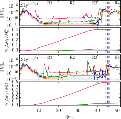
Figure 15: Hamiltonian constraint (first and third panel) and rest mass conservation (second and fourth panel) for the SLy^(↙↘)case (top) and the SLy^(↗↗)case (bottom). The merger time, corresponding to the peak in the (2,2)-mode of GW strain is shown as vertical dashed line for each resolution.

Constraint violation and mass conservation:-

For assessing the accuracy and robustness of our simulations, we present the $L_{2}$ volume norm of the Hamiltonian constraint and the conservation of rest mass in Fig. 15 for the SLy^(↙↘)case (top panels) and for the SLy^(↗↗)case (botton panels).

Owing to the constraint propagation and damping properties of the Z4c evolution system the constraint stays at or below the value of the initial data. Oscillations and spikes in the constraints during the orbital motion, as seen in Fig. 15, mainly originate due the inner refinement levels following the motion of the NSs. After the merger (vertical dashed lines), those spikes are absent as the stars stay near the center or move with a very small velocity compared to during the inspiral phase. At merger the constraint grows by about two orders of magnitude due to regridding and to the development of large gradients in the solution, but it remains below the initial level. Subsequently, the violation is again propagated away and damped. Throughout the simulation we find that the Hamiltonian constraint violation improves monotonically with increasing resolution for the SLy^(↙↘)case. For the SLy^(↗↗)case, only the lower three resolutions, R1, R2 and R3 show this trend whereas for the highest resolution R4, the constraint violation grows one order of magnitude at $t=~{}22\rm ms$ during the regridding of the grid, but does not decrease afterwards; the exact origin of this effect is currently under investigation, but it seems that the results presented in the main text are unaffected; cf. also Fig. 16.

Violations of rest-mass conservation, shown in Fig. 15, happen at the mesh refinement boundaries and due to the artificial atmosphere treatment, and possibly due to mass leaving the computational domain. From the time evolution of the mass violation, we find that, independent of the spin orientation, the resolution R1 shows an increasing mass during the orbital motion. This is caused by inadequate resolution and the artificial atmosphere treatment, see e.g. Dietrich et al. (2015b). For resolutions R2, R3, and R4 the rest mass stays constant within $0.1\%$ throughout the simulation time. The mass loss is caused by the ejected material which decompresses while it leaves the central region of the numerical domain. Once the density drops by $12$ orders of magnitude, the material is counted as atmosphere and is not evolved further. Consequently, conservation of total mass is violated. Overall the mass violation is below $0.6\%$ considering all the resolutions employed in this article.

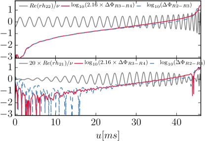
Figure 16: Real part of the (2,2) mode (top panel) and (2,1) mode (bottom panel) for resolution R4 as well as the phase difference between different resolutions for the SLy^(↗↗)configuration shown versus retarded time. We multiply the amplitude of the (2,1) mode by a factor of $20$ for better visibility.

Waveform accuracy:-

In Fig. 16 we present the GW phase difference between different resolutions for SLy^(↗↗)during the inspiral up to the moment of merger, which we define as the time of maximum amplitude in the (2,2)-mode. Through the inspiral we see a monotonic decrease of the phase difference for increasing resolution. Note that in Fig. 16 we have scaled the phase difference from R3-R4 assuming second-order convergence. We find that the rescaled curve agrees very well with the R2-R3 curve implying that our results are in the convergent regime with increasing resolution.

References

- Abbott et al. (2017a) B. P. Abbott et al. (LIGO Scientific Collaboration and Virgo Collaboration), Phys. Rev. Lett. 119, 161101 (2017a), arXiv:1710.05832 [gr-qc] .
- Abbott et al. (2017b) B. P. Abbott et al. (LIGO Scientific Collaboration, Virgo Collaboration, Fermi Gamma-ray Burst Monitor, and INTEGRAL), Astrophys. J. Lett. 848, L13 (2017b), arXiv:1710.05834 [astro-ph.HE] .
- Abbott et al. (2017c) B. P. Abbott et al. (LIGO Scientific, VINROUGE, Las Cumbres Observatory, DLT40, Virgo, 1M2H, MASTER), Nature (2017c), 10.1038/nature24471, arXiv:1710.05835 [astro-ph.CO] .
- Coughlin et al. (2019a) M. W. Coughlin, T. Dietrich, J. Heinzel, N. Khetan, S. Antier, N. Christensen, D. A. Coulter, and R. J. Foley, (2019a), arXiv:1908.00889 [astro-ph.HE] .
- Cowperthwaite et al. (2017) P. S. Cowperthwaite et al., Astrophys. J. 848, L17 (2017), arXiv:1710.05840 [astro-ph.HE] .
- Smartt et al. (2017) S. J. Smartt et al., Nature (2017), 10.1038/nature24303, arXiv:1710.05841 [astro-ph.HE] .
- Kasliwal et al. (2017) M. M. Kasliwal et al., (2017), 10.1126/science.aap9455, arXiv:1710.05436 [astro-ph.HE] .
- Kasen et al. (2017) D. Kasen, B. Metzger, J. Barnes, E. Quataert, and E. Ramirez-Ruiz, Nature (2017), 10.1038/nature24453, [Nature551,80(2017)], arXiv:1710.05463 [astro-ph.HE] .
- Watson et al. (2019) D. Watson et al., Nature 574, 497 (2019), arXiv:1910.10510 [astro-ph.HE] .
- Abbott et al. (2019a) B. P. Abbott et al. (LIGO Scientific, Virgo), Phys. Rev. X9, 011001 (2019a), arXiv:1805.11579 [gr-qc] .
- Radice and Dai (2019) D. Radice and L. Dai, Eur. Phys. J. A55, 50 (2019), arXiv:1810.12917 [astro-ph.HE] .
- Coughlin et al. (2019b) M. W. Coughlin, T. Dietrich, B. Margalit, and B. D. Metzger, Mon. Not. Roy. Astron. Soc. 489, L91 (2019b), arXiv:1812.04803 [astro-ph.HE] .
- Capano et al. (2019) C. D. Capano, I. Tews, S. M. Brown, B. Margalit, S. De, S. Kumar, D. A. Brown, B. Krishnan, and S. Reddy, (2019), arXiv:1908.10352 [astro-ph.HE] .
- Dietrich et al. (2020) T. Dietrich, M. W. Coughlin, P. T. H. Pang, M. Bulla, J. Heinzel, L. Issa, I. Tews, and S. Antier, (2020), arXiv:2002.11355 [astro-ph.HE] .
- Abbott et al. (2020) B. P. Abbott et al. (LIGO Scientific, Virgo), (2020), arXiv:2001.01761 [astro-ph.HE] .
- Veitch et al. (2015) J. Veitch et al., Phys. Rev. D 91, 042003 (2015), arXiv:1409.7215 [gr-qc] .
- Kiziltan et al. (2013) B. Kiziltan, A. Kottas, M. De Yoreo, and S. E. Thorsett, Astrophys. J. 778, 66 (2013), arXiv:1309.6635 [astro-ph.SR] .
- Lattimer (2012) J. M. Lattimer, Ann. Rev. Nucl. Part. Sci. 62, 485 (2012), arXiv:1305.3510 [nucl-th] .
- Lorimer (2008) D. R. Lorimer, Living Rev. Rel. 11, 8 (2008), arXiv:0811.0762 [astro-ph] .
- Farr et al. (2011) W. M. Farr, K. Kremer, M. Lyutikov, and V. Kalogera, Astrophys. J. 742, 81 (2011), arXiv:1104.5001 [astro-ph.HE] .
- Bernuzzi et al. (2014) S. Bernuzzi, T. Dietrich, W. Tichy, and B. Brügmann, Phys. Rev. D 89, 104021 (2014), arXiv:1311.4443 [gr-qc] .
- Dietrich et al. (2015a) T. Dietrich, N. Moldenhauer, N. K. Johnson-McDaniel, S. Bernuzzi, C. M. Markakis, B. Brügmann, and W. Tichy, Phys. Rev. D 92, 124007 (2015a), arXiv:1507.07100 [gr-qc] .
- Dietrich et al. (2017a) T. Dietrich, S. Bernuzzi, M. Ujevic, and W. Tichy, Phys. Rev. D 95, 044045 (2017a), arXiv:1611.07367 [gr-qc] .
- Dietrich et al. (2018a) T. Dietrich, S. Bernuzzi, B. Bruegmann, and W. Tichy (2018) arXiv:1803.07965 [gr-qc] .
- Most et al. (2019) E. R. Most, L. J. Papenfort, A. Tsokaros, and L. Rezzolla, Astrophys. J. 884, 40 (2019), arXiv:1904.04220 [astro-ph.HE] .
- Tsokaros et al. (2019) A. Tsokaros, M. Ruiz, V. Paschalidis, S. L. Shapiro, and K. Uryū, Phys. Rev. D 100, 024061 (2019), arXiv:1906.00011 [gr-qc] .
- East et al. (2019) W. E. East, V. Paschalidis, F. Pretorius, and A. Tsokaros, Phys. Rev. D 100, 124042 (2019), arXiv:1906.05288 [astro-ph.HE] .
- Tacik et al. (2015) N. Tacik et al., Phys. Rev. D 92, 124012 (2015), 94, 049903(E) (2016), arXiv:1508.06986 [gr-qc] .
- Dietrich et al. (2018b) T. Dietrich, S. Bernuzzi, B. Brügmann, M. Ujevic, and W. Tichy, Phys. Rev. D 97, 064002 (2018b), arXiv:1712.02992 [gr-qc] .
- Tichy (2006) W. Tichy, Phys. Rev. D 74, 084005 (2006), arXiv:gr-qc/0609087 [gr-qc] .
- Tichy (2009a) W. Tichy, Classical Quantum Gravity 26, 175018 (2009a), arXiv:0908.0620 [gr-qc] .
- Tichy (2009b) W. Tichy, Phys. Rev. D 80, 104034 (2009b), arXiv:0911.0973 [gr-qc] .
- Tichy et al. (2019) W. Tichy, A. Rashti, T. Dietrich, R. Dudi, and B. Brügmann, Phys. Rev. D 100, 124046 (2019), arXiv:1910.09690 [gr-qc] .
- Wilson and Mathews (1995) J. Wilson and G. Mathews, Phys. Rev. Lett. 75, 4161 (1995).
- Wilson et al. (1996) J. Wilson, G. Mathews, and P. Marronetti, Phys. Rev. D 54, 1317 (1996), arXiv:gr-qc/9601017 [gr-qc] .
- York Jr. (1999) J. W. York Jr., Phys. Rev. Lett. 82, 1350 (1999), arXiv:gr-qc/9810051 [gr-qc] .
- Tichy (2011) W. Tichy, Phys. Rev. D 84, 024041 (2011), arXiv:1107.1440 [gr-qc] .
- Tichy (2012) W. Tichy, Phys. Rev. D 86, 064024 (2012), arXiv:1209.5336 [gr-qc] .
- Tichy (2017) W. Tichy, Rept. Prog. Phys. 80, 026901 (2017), arXiv:1610.03805 [gr-qc] .
- Brügmann et al. (2008) B. Brügmann, J. A. Gonzalez, M. Hannam, S. Husa, U. Sperhake, and W. Tichy, Phys. Rev. D 77, 024027 (2008), arXiv:gr-qc/0610128 [gr-qc] .
- Thierfelder et al. (2011) M. Thierfelder, S. Bernuzzi, and B. Brügmann, Phys. Rev. D 84, 044012 (2011), arXiv:1104.4751 [gr-qc] .
- Dietrich et al. (2015b) T. Dietrich, S. Bernuzzi, M. Ujevic, and B. Brügmann, Phys. Rev. D 91, 124041 (2015b), arXiv:1504.01266 [gr-qc] .
- Bernuzzi and Dietrich (2016) S. Bernuzzi and T. Dietrich, Phys. Rev. D 94, 064062 (2016), arXiv:1604.07999 [gr-qc] .
- Bernuzzi and Hilditch (2010) S. Bernuzzi and D. Hilditch, Phys. Rev. D 81, 084003 (2010), arXiv:0912.2920 [gr-qc] .
- Hilditch et al. (2013) D. Hilditch, S. Bernuzzi, M. Thierfelder, Z. Cao, W. Tichy, et al., Phys. Rev. D 88, 084057 (2013), arXiv:1212.2901 [gr-qc] .
- Bona et al. (1996) C. Bona, J. Massó, J. Stela, and E. Seidel, in The Seventh Marcel Grossmann Meeting: On Recent Developments in Theoretical and Experimental General Relativity, Gravitation, and Relativistic Field Theories, edited by R. T. Jantzen, G. M. Keiser, and R. Ruffini (World Scientific, Singapore, 1996).
- Alcubierre et al. (2003) M. Alcubierre, B. Brügmann, P. Diener, M. Koppitz, D. Pollney, E. Seidel, and R. Takahashi, Phys. Rev. D 67, 084023 (2003), arXiv:gr-qc/0206072 [gr-qc] .
- van Meter et al. (2006) J. R. van Meter, J. G. Baker, M. Koppitz, and D.-I. Choi, Phys. Rev. D 73, 124011 (2006), arXiv:gr-qc/0605030 .
- Borges et al. (2008) R. Borges, M. Carmona, B. Costa, and W. S. Don, J. Comput. Phys. 227, 3191 (2008).
- Jiang (1996) G. Jiang, J. Comp. Phys. 126, 202 (1996).
- Suresh (1997) A. Suresh, J. Comp. Phys. 136, 83 (1997).
- Mignone et al. (2010) A. Mignone, P. Tzeferacos, and G. Bodo, J.Comput.Phys. 229, 5896 (2010), arXiv:1001.2832 [astro-ph.HE] .
- Read et al. (2009) J. S. Read, C. Markakis, M. Shibata, K. Uryū, J. D. Creighton, and J. L. Friedman, Phys. Rev. D 79, 124033 (2009), arXiv:0901.3258 [gr-qc] .
- Bauswein et al. (2010) A. Bauswein, H.-T. Janka, and R. Oechslin, Phys. Rev. D 82, 084043 (2010), arXiv:1006.3315 [astro-ph.SR] .
- Berger and Oliger (1984) M. J. Berger and J. Oliger, J. Comput. Phys. 53, 484 (1984).
- Abbott et al. (2019b) B. P. Abbott et al. (LIGO Scientific, Virgo), Phys. Rev. X 9, 031040 (2019b), arXiv:1811.12907 [astro-ph.HE] .
- Morsink and Stella (1999) S. M. Morsink and L. Stella, The Astrophysical Journal 513, 827 (1999).
- Campanelli et al. (2006) M. Campanelli, C. Lousto, and Y. Zlochower, Phys. Rev. D 74, 041501 (2006), arXiv:gr-qc/0604012 [gr-qc] .
- (59) http://www.computational-relativity.org/, CoRe database of binary neutron star merger waveforms.
- Dietrich et al. (2018c) T. Dietrich, D. Radice, S. Bernuzzi, F. Zappa, A. Perego, B. Brügmann, S. V. Chaurasia, R. Dudi, W. Tichy, and M. Ujevic, (2018c), arXiv:1806.01625 [gr-qc] .
- Kidder et al. (1993) L. E. Kidder, C. M. Will, and A. G. Wiseman, Phys. Rev. D 47, 4183 (1993), arXiv:gr-qc/9211025 [gr-qc] .
- Kastaun and Galeazzi (2015) W. Kastaun and F. Galeazzi, Phys. Rev. D 91, 064027 (2015), arXiv:1411.7975 [gr-qc] .
- Kastaun et al. (2013) W. Kastaun, F. Galeazzi, D. Alic, L. Rezzolla, and J. A. Font, Phys. Rev. D 88, 021501 (2013), arXiv:1301.7348 [gr-qc] .
- East and Pretorius (2012) W. E. East and F. Pretorius, Astrophys. J. Lett. 760, L4 (2012), arXiv:1208.5279 [astro-ph.HE] .
- Kastaun et al. (2017) W. Kastaun, R. Ciolfi, A. Endrizzi, and B. Giacomazzo, Phys. Rev. D 96, 043019 (2017), arXiv:1612.03671 [astro-ph.HE] .
- Chaurasia et al. (2018) S. V. Chaurasia, T. Dietrich, N. K. Johnson-McDaniel, M. Ujevic, W. Tichy, and B. Brügmann, Phys. Rev. D 98, 104005 (2018), arXiv:1807.06857 [gr-qc] .
- Gonzalez et al. (2007) J. A. Gonzalez, M. D. Hannam, U. Sperhake, B. Brügmann, and S. Husa, Phys. Rev. Lett. 98, 231101 (2007), arXiv:gr-qc/0702052 [GR-QC] .
- Brügmann et al. (2008) B. Brügmann, J. A. González, M. Hannam, S. Husa, and U. Sperhake, Physical Review D 77 (2008), 10.1103/physrevd.77.124047.
- González et al. (2007) J. A. González, U. Sperhake, B. Brügmann, M. Hannam, and S. Husa, Phys. Rev. Lett. 98, 091101 (2007), arXiv:gr-qc/0610154 .
- Dietrich et al. (2019a) T. Dietrich et al., Phys. Rev. D 99, 024029 (2019a), arXiv:1804.02235 [gr-qc] .
- Dietrich et al. (2019b) T. Dietrich, A. Samajdar, S. Khan, N. K. Johnson-McDaniel, R. Dudi, and W. Tichy, Phys. Rev. D 100, 044003 (2019b), arXiv:1905.06011 [gr-qc] .
- Khan et al. (2016) S. Khan, S. Husa, M. Hannam, F. Ohme, M. Pürrer, X. Jiménez Forteza, and A. Bohé, Phys. Rev. D 93, 044007 (2016), arXiv:1508.07253 [gr-qc] .
- Husa et al. (2016) S. Husa, S. Khan, M. Hannam, M. Pürrer, F. Ohme, X. Jiménez Forteza, and A. Bohé, Phys. Rev. D 93, 044006 (2016), arXiv:1508.07250 [gr-qc] .
- Schmidt et al. (2012) P. Schmidt, M. Hannam, and S. Husa, Phys. Rev. D 86, 104063 (2012), arXiv:1207.3088 [gr-qc] .
- Schmidt et al. (2015) P. Schmidt, F. Ohme, and M. Hannam, Phys. Rev. D 91, 024043 (2015), arXiv:1408.1810 [gr-qc] .
- Takami et al. (2014) K. Takami, L. Rezzolla, and L. Baiotti, Phys. Rev. Lett. 113, 091104 (2014), arXiv:1403.5672 [gr-qc] .
- Dietrich (2016) T. Dietrich, Binary neutron star merger simulations, Ph.D. thesis, Jena (2016), dissertation, Friedrich-Schiller-Universität Jena, 2016.
- Tsang et al. (2019) K. W. Tsang, T. Dietrich, and C. Van Den Broeck, Physical Review D 100 (2019), 10.1103/physrevd.100.044047.
- Breschi et al. (2019) M. Breschi, S. Bernuzzi, F. Zappa, M. Agathos, A. Perego, D. Radice, and A. Nagar, Physical Review D 100 (2019), 10.1103/physrevd.100.104029.
- Bauswein et al. (2016) A. Bauswein, N. Stergioulas, and H.-T. Janka, Eur. Phys. J. A52, 56 (2016), arXiv:1508.05493 [astro-ph.HE] .
- Dietrich et al. (2017b) T. Dietrich, M. Ujevic, W. Tichy, S. Bernuzzi, and B. Brügmann, Phys. Rev. D 95, 024029 (2017b), arXiv:1607.06636 [gr-qc] .
- Alcubierre (2008) M. Alcubierre, Introduction to 3+1 Numerical Relativity, by Miguel Alcubierre. ISBN 978-0-19-920567-7 (HB). Published by Oxford University Press, Oxford, UK, 2008., edited by M. Alcubierre (Oxford University Press, 2008).