The most powerful astrophysical events: Gravitational-wave peak
luminosity of binary black holes as predicted by numerical relativity

Abstract

For a brief moment, a binary black hole (BBH) merger can be the most powerful astrophysical event in the visible Universe. Here we present a model fit for this gravitational-wave peak luminosity of nonprecessing quasicircular BBH systems as a function of the masses and spins of the component black holes, based on numerical relativity (NR) simulations and the hierarchical fitting approach introduced by X. Jiménez Forteza et al. [Phys. Rev. D 95, 064024 (2017)]. This fit improves over previous results in accuracy and parameter-space coverage and can be used to infer posterior distributions for the peak luminosity of future astrophysical signals like GW150914 and GW151226. The model is calibrated to the $\ell\leq 6$ modes of 378 nonprecessing NR simulations up to mass ratios of 18 and dimensionless spin magnitudes up to 0.995, and includes unequal-spin effects. We also constrain the fit to perturbative numerical results for large mass ratios. Studies of key contributions to the uncertainty in NR peak luminosities, such as (i) mode selection, (ii) finite resolution, (iii) finite extraction radius, and (iv) different methods for converting NR waveforms to luminosity, allow us to use NR simulations from four different codes as a homogeneous calibration set. This study of systematic fits to combined NR and large-mass-ratio data, including higher modes, also paves the way for improved inspiral-merger-ringdown waveform models.

published journal version:
Phsyical Review D 96, 024006 (2017)
doi:10.1103/PhysRevD.96.024006

I Introduction

With Advanced LIGO’s Aasi et al. (2015); Abbott et al. (2016a) first detections Abbott et al. (2016b, c, d), binary black hole (BBH) coalescences have become objects of observational astronomy. The peak rate at which BBHs radiate gravitational wave (GW) energy makes them the most luminous known phenomena in the Universe. The source of the first GW detection GW150914 has been inferred to be consistent with two black holes (BHs) of $29_{-4}^{+4}\,M_{\odot}$ and $36_{-4}^{+5}\,M_{\odot}$ inspiraling, merging and ringing down as described by General Relativity (GR). Its emission of GW energy reached, for a small fraction of a second, a peak rate of $3.6_{-0.4}^{+0.5}\times 10^{56}{}$ erg/s, equivalent to $200_{-20}^{+30}\,M_{\odot}\,c^{2}/\mathrm{s}$ Abbott et al. (2016b, e, f).

Though this peak luminosity, $L_{\mathrm{peak}}$, is not electromagnetic, but gravitational, we can compare its numerical value to the photon luminosity of other astrophysical sources to illustrate its scale: GW150914 at its peak emitted as much power as ${\sim}10^{23}$ suns, $\gtrsim 10^{11}$ times more than all stars in the Milky Way, and still 60–90 times more than the ultra-luminous gamma-ray burst GRB 110918A Frederiks et al. (2013).

The peak luminosities for LIGO’s first BBH events were inferred using a fit Jiménez Forteza et al. (2016) to data from numerical relativity (NR) simulations, which we will improve upon in this paper through an enhanced fitting method and a significantly larger calibration data set. Source parameters of GW events are determined through Bayesian inference Aasi et al. (2013); Veitch et al. (2015); Abbott et al. (2016e, d, g), comparing LIGO data with waveform models, which are approximate maps between the masses and spins of the binary components and the GW signal. As of the aLIGO O1 run, the state-of-the-art NR-calibrated BBH waveform models were PhenomPv2 Hannam et al. (2014); Bohé et al. (2016, ) (a precessing model based on the aligned-spin PhenomD Husa et al. (2016); Khan et al. (2016)) and SEOBNRv2/3 Pan et al. (2014); Pürrer (2014, 2016); Abbott et al. (2016g); Babak et al. (2017). A detailed recent study Abbott et al. (2017) has found these models to be at least sufficiently accurate in the parameter region corresponding to the first detection.

The primary products of this inference are multidimensional sample chains that approximate posterior probability density functions (PDFs) for the intrinsic and extrinsic BBH parameters. Subsequently, such a sampled PDF can be used to infer other quantities, typically obtained through fitting formulas calibrated to NR. Examples include final-state properties Healy et al. (2014); Husa et al. (2016); Healy and Lousto (2017); Hofmann et al. (2016); Jiménez-Forteza et al. (2017): the final spin and final mass of the merger remnant, a single Kerr BH, which also yield the total radiated energy. In fact, full inspiral-merger-ringdown waveform models include such final-state NR fits to describe the ringdown phase, but due to practical implementation details and for greater flexibility in using updated fits, the values reported in Refs. Abbott et al. (2016b, c, d, g) come from stand-alone fitting formulas evaluated on posterior PDFs.

The same approach is used for inference of the GW peak luminosity. However, a robust $L_{\mathrm{peak}}$ model for general BBH configurations was not available in the literature prior to O1. An early phenomenological formula Baker et al. (2008) is limited to nonspinning BBHs, and thus a new fit Jiménez Forteza et al. (2016) had to be developed. To accurately capture the luminosities of the NR calibration set, it also took into account contributions from subdominant harmonics not included in most current waveform models.

In this paper, we present an improved version of that model fit for the GW peak luminosity from the merger of more general BBH systems, including spins on both binary components. Still, we concentrate on cases where the spin of each BH is aligned with the system’s total angular momentum, using the dimensionless components $\chi_{i}=S_{i}/m_{i}^{2}=\tfrac{\vec{S}_{i}}{m_{i}^{2}}\cdot\tfrac{\vec{L}}{|\vec{L}|}$ of the spins $\vec{S}_{i}$ projected onto the orbital angular momentum $\vec{L}$. We use the hierarchical data-driven approach introduced in Ref. Jiménez-Forteza et al. (2017) to develop a three-dimensional ansatz and fit it to a total of 378 simulations from four separate NR codes, including more subdominant modes than before, and to independent numerical results for large mass ratios obtained with the perturbative scheme of Refs. Nagar et al. (2007); Bernuzzi et al. (2011a); Harms et al. (2014). This addition is essential in producing a well-constrained fit at very unequal masses where NR coverage is sparse or nonexistent.

Notably, the GW peak luminosity $L_{\mathrm{peak}}$ does not depend on the total mass of a BBH system: luminosity generally scales with emitted energy over emission time scale, $L\sim E_{\mathrm{rad}}/\Delta t$. But for a BBH, both the total radiated energy $E_{\mathrm{rad}}$ and the characteristic merger time scale $\Delta t$ are proportional to the total mass, so that $L_{\mathrm{peak}}$ is independent of it. Hence, the GW peak luminosities even of super-massive black hole (SMBH) binaries, observable by eLISA-like missions Amaro Seoane et al. (2013a, b); Klein et al. (2016) or by pulsar timing arrays (PTAs, Rajagopal and Romani (1995); Sesana et al. (2009); Sesana and Vecchio (2010)), are similar to those of stellar-mass BBHs. The results of this paper will be applicable to such systems as well.

Besides using $L_{\mathrm{peak}}$ to compare the energetics of GWs and other astrophysical events, one can also consider its relevance for the effect of BBH coalescences on their immediate surroundings. The influence of SMBH mergers on circumbinary accretion disks (see Ref. Schnittman (2013) and references therein) is determined mostly by the integrated radiated energy of the late-inspiral and merger phase, though the authors of Refs. Kocsis and Loeb (2008); Li et al. (2012) suggested weak prompt electromagnetic counterparts sensitive to $L_{\mathrm{peak}}$ and $L_{\mathrm{GW}}(t)$. For stellar-mass BBHs, any significant interaction with surrounding material or fields is highly speculative – see e.g. the references in Sec. 4 of Ref. Connaughton et al. (2016). Still it is conceivable that an accurate $L_{\mathrm{peak}}$ model could be useful in constraining exotic models.

Turning $L_{\mathrm{peak}}$ into an independent GW observable through direct signal reconstruction Cornish and Littenberg (2015); Klimenko et al. (2016); Lynch et al. (2017); Bécsy et al. (2017); Abbott et al. (2016h) will require improved detector sensitivity and calibration accuracy, so that the peak strain can be measured to high absolute accuracy and that degeneracies between the distance estimate and other parameters are significantly reduced. Currently, NR-calibrated fits are the only accurate method to infer peak luminosities from GW observations.

Another motivation for this improved fit is its role as a test case of the general fitting method from Ref. Jiménez-Forteza et al. (2017) for quantities that require accurate treatment of the higher modes from NR simulations, and of combining NR and perturbative large-mass-ratio results. In these aspects, the present study is a preparation for the development of improved inspiral-merger-ringdown waveform models.

In this paper, we use geometric units with $G=1$, $c=1$ and unit total mass $M$, so that luminosity is a dimensionless quantity, corresponding to $1M$ of energy radiated per $1M$ of time. The conversion factor to Watt is $c^{5}/G$, and another factor $10^{7}$ for the usual astronomical unit of erg/s. We will first review the catalog of NR simulations of BBH mergers and perturbative large-mass-ratio data used to construct our model in Sec. II. We discuss the challenges in combining NR data from different simulation codes, the steps taken to process the different sets into a single, effectively homogeneous data set, and how this set is augmented with independent results for large-mass-ratio systems. Given this data set, we discuss the construction and validation of our model fit for peak luminosity in Secs. III and IV. We also compare our new fit with the previous result of Ref. Jiménez Forteza et al. (2016), calibrated to a smaller NR data set, that was used during O1 Abbott et al. (2016b, c, d, e, g); and to another independent, recently published fit Healy and Lousto (2017). The Appendix includes more details on investigations of the NR data.

II Input data

II.1 Numerical relativity data sets

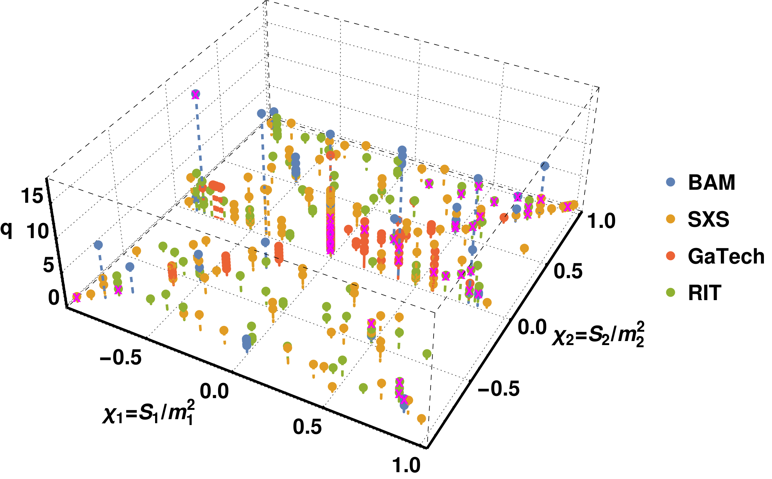
Figure 1: Parameter-space coverage of the combined NR data set from BAM, SXS, GaTech, and RIT, shown against the individual BH spins and the mass ratio $q=m_{1}/m_{2}$ of the system. Simulations not used in the fit (see Table 6) are marked with magenta crosses.

We begin by considering 419 nonprecessing NR simulations from four sources, with their coverage of the three-dimensional BBH parameter space illustrated in Figs. 1 and 2:

1. 47 simulations performed by the authors with the BAM code Bruegmann et al. (2008); Husa et al. (2008), including those first used in Refs. Husa et al. (2016); Jiménez-Forteza et al. (2017).

2. 160 simulations from the public SXS catalog Mroué et al. (2013); SXS Collaboration (2016a) performed with the Spectral Einstein Code (SpEC) SXS Collaboration (2016b).

3. 105 simulations from the public GaTech catalog Jani et al. (2016a, b), performed with the MAYA code Herrmann et al. (2007); Vaishnav et al. (2007); Healy et al. (2009); Pekowsky et al. (2013a).

4. 107 simulations Healy et al. (2014); Healy and Lousto (2017); Healy et al. (2017); Campanelli et al. (2016) with the LAZEV code Zlochower et al. (2005), labeled “RIT” in the following.

BAM, MAYA and LAZEV are finite difference codes to solve the Baumgarte-Shapiro-Shibata-Nakamura formulation of the GR initial value problem Baumgarte and Shapiro (1998) with a singularity-avoiding slicing condition following the moving puncture approach Campanelli et al. (2006); Baker et al. (2006), whereas the simulations of the SXS Collaboration have been performed with the pseudospectral SpEC code SXS Collaboration (2016b) which employs the generalized harmonic gauge (GHG) combined with black-hole excision.

We use mass and spin parameters of the component BHs after equilibration and the initial burst of “junk“ radiation. To compute the luminosity for BAM, SXS and GaTech simulations, we begin with the Weyl scalar $\psi_{4}$ decomposed into its spin-two spherical harmonic multipoles,

$$\psi_{\ell m}(t)\;=\;\frac{1}{r}\,\int_{\Omega}\,{}_{-2}\overline{Y}_{\ell m}(\theta,\phi)\,\psi_{4}(t,\theta,\phi)\,\mathrm{d}\Omega\;.$$ ((1))

For SXS $\psi_{4}$ data, we have applied corrections for center-of-mass drifts Boyle (2013); Boyle et al. (2014); Boyle (2016), which remove some unphysical oscillations in higher modes. From these spherical harmonic multipoles, we calculate the GW strain-rate multipoles $\dot{h}_{\ell m}(t)$ via the fixed-frequency-integration (FFI) method described in Ref. Reisswig and Pollney (2011). We then compute the peak luminosity according to

$$L_{\mathrm{peak}}=\mathop{\mathrm{max}}_{t}\;\lim_{r\rightarrow\infty}\frac{r^{2}}{16\,\pi}\sum_{\ell=2}^{\ell_{\max}}\sum_{m=-\ell}^{+\ell}\left|\,\dot{h}_{\ell m}(t)\,\right|^{2}\,,$$ ((2))

truncating the sum over $\ell$ at $\ell_{\max}=6$. For RIT simulations, we use directly the peak luminosity values as given in Ref. Healy and Lousto (2017), which again include all modes up to $\ell_{\max}=6$.

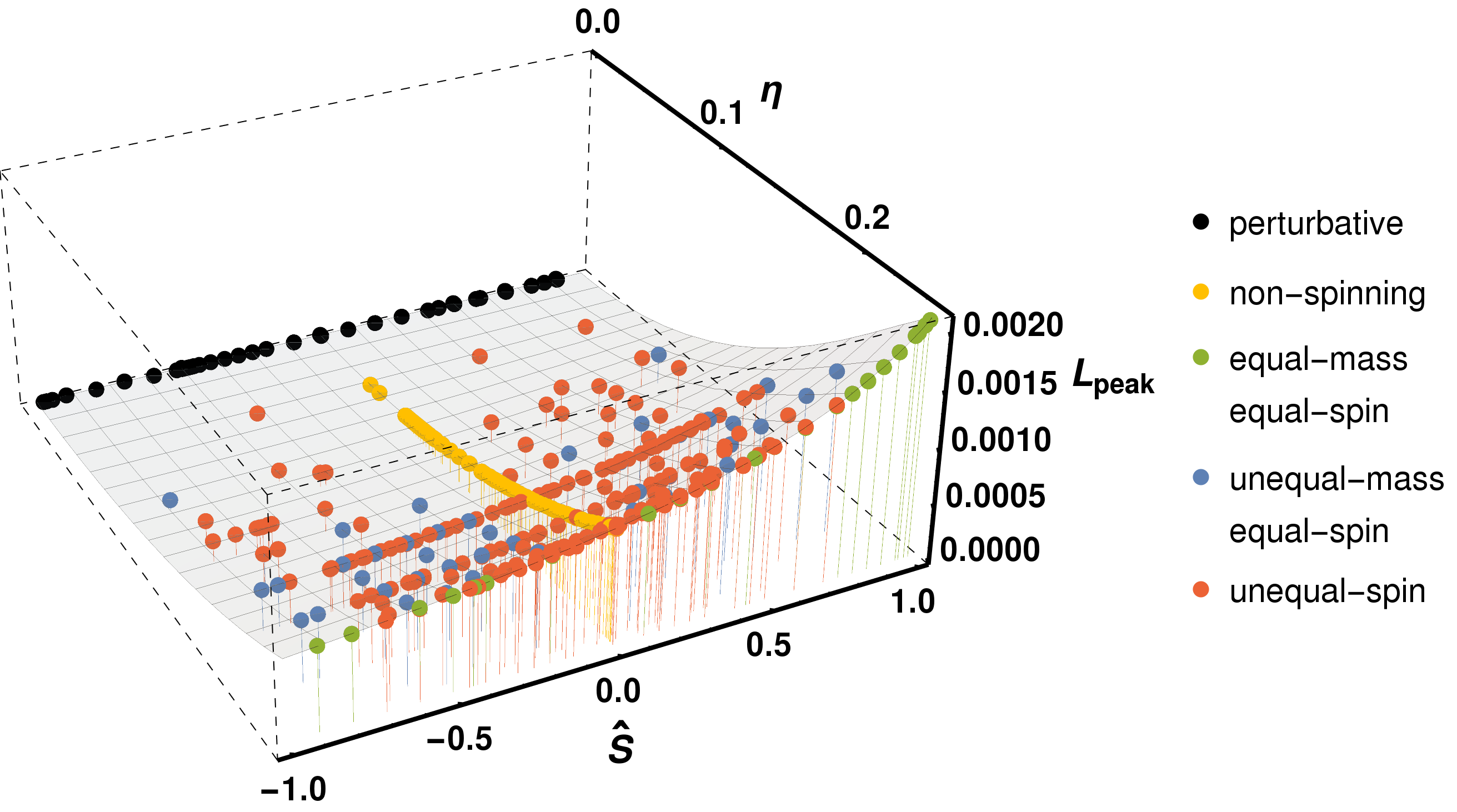
Figure 2: Combined data set over the two-dimensional space spanned by symmetric mass ratio $\eta$ and effective spin $\widehat{S}$, defined in Eq. (3). Top panel: peak luminosity $L_{\mathrm{peak}}$. Lower panel: rescaled as $L_{\mathrm{peak}}/\eta^{2}L_{0}$. Subsets used in the various steps of Sec. III are highlighted by colors. The shaded surface is added here to guide the eye, but is in fact the 2D projection of the new fit developed in this paper.

NR simulation results always have finite accuracy, and the post-processing from the initial $\psi_{4}(t,\theta,\phi)$ to the final product $L_{\mathrm{peak}}$ can lead to additional sources of inaccuracies that could substantially affect the accuracy of individual data points and of any NR-calibrated fits. As we aim to fit small subdominant effects, such as those of unequal spins, possible error sources must be carefully analyzed. Thus, we have considered the impact of the following effects on $L_{\mathrm{peak}}$, with details on each aspect given in the Appendix:

1. Conversion between strain $h(t)$, $\psi_{4}(t)$ and luminosity $L(t)$: The FFI approach is known to be accurate at the $1\%$ level or better. Reisswig and Pollney (2011) We have also tested its validity by verifying that it agrees with a newly developed alternative technique to compute $h(t)$ and $L(t)$ from the time-domain $\psi_{4}(t)$.

2. Extrapolation effects: Gauge invariability of the waveforms is only well defined for an observer at null infinity. We have extrapolated $L_{\mathrm{peak}}$, as computed from waveforms available at a range of finite extraction radii, to infinity and estimated the extrapolation uncertainty.

3. Finite resolution: Convergence tests are only available for a small subset of NR configurations, with estimates indicating that errors due to finite grid resolution are a nondominant but non-negligible contribution to the total error budget.

4. Peak accuracy and discreteness: The peak in luminosity can be quite steep, but we have verified that with a sampling of 0.1M in time the difference between two points next to the peak is only on the order of 0.01–0.2%.

5. Mode selection: While the $\ell=|m|=2$ mode has the largest peak amplitude for all mass ratios, the importance of other spherical harmonics monotonically increases toward the extreme-mass-ratio limit. We can thus bound higher-mode contributions by comparison with the large-mass-ratio results, where neglecting modes with $\ell>8$ incurs an error below 1% even for mass ratios of $10^{5}$ (see below in Sec. II.2). For the available NR waveforms, we determine that it is generally sufficient to consider modes up to $\ell_{\max}=6$, with contributions of the $\ell=7,8$ modes rising to only 1% for mass ratio 18 nonspinning cases.

We remove 41 cases from the initial catalog for reasons as discussed in the Appendix, e.g. because they are inconsistent with equivalent or nearby configurations from the same or other codes. Thus, we perform our fit with a final set of 378 NR results.

II.2 Perturbative large-mass-ratio data

As the computational cost of NR simulations increases rapidly for unequal mass ratios, no data for BBH systems with mass ratios $q>18$ are currently available from any of the simulation codes discussed above. ( $q=m_{1}/m_{2}$ with the convention $m_{1}>m_{2}$.) However, constraining fits to some known behavior in or close to the extreme-mass-ratio limit is essential in ensuring a sane extrapolation towards that limit, and also to reduce uncertainty in the intermediate-mass-ratio region where there is some NR coverage, but it is still very sparse.

For the final-state quantities studied in Ref. Jiménez-Forteza et al. (2017), we used analytical expressions from Ref. Bardeen et al. (1972) for the limiting case of a test particle orbiting a Kerr black hole. For the peak luminosity, it is known Teukolsky and Press (1974); Fujita (2015) that the leading-order term as $\eta\rightarrow 0$ must be $L_{\mathrm{peak}}\propto\eta^{2}$, with the symmetric mass ratio $\eta=(m_{1}m_{2})/(m_{1}+m_{2})^{2}=q/(1+q)^{2}$. However, no fully analytical results for the spin dependence in the extreme-mass-ratio limit exist. Instead, here we constrain our fit by numerical results for finite, but very large mass ratios.

The simulation method for BBH mergers in the test-mass (large-mass-ratio) limit developed in Refs. Nagar et al. (2007); Bernuzzi and Nagar (2010); Harms et al. (2014) combines a semianalytical description of the dynamics with a time-domain numerical approach for computing the multipolar waveform based on BH perturbation theory. The small BH’s dynamics are prescribed using the effective-one-body (EOB) test-mass dynamics, i.e. the conservative (geodesic) motion augmented with a linear-in-$\eta$ radiation reaction expression Nagar et al. (2007); Damour and Nagar (2007). The latter is built from the factorized and resummed circularized waveform introduced in Ref. Damour et al. (2009) (and Ref. Pan et al. (2011) for spin) and uses Post-Newtonian (PN) information up to 5.5PN (see also Refs. Fujita (2012); Nagar and Shah (2016) for extensions up to 22PN). Waveforms are calculated by solving either the Regge-Wheeler-Zerilli (RWZ) 1+1 equations (nonspinning case) or the Teukolsky 2+1 equation (spinning case). Those equations are solved in the time-domain using hyperboloidal coordinates to extract the radiation unambiguously at scri (null infinity) Bernuzzi et al. (2011b, a); Harms et al. (2014).

The method has been extensively applied for developing and assessing the quality of EOB waveforms Bernuzzi et al. (2011a); Harms et al. (2014), informing the EOB model in the test-mass limit Damour et al. (2013), quasinormal mode excitation Bernuzzi and Nagar (2010); Harms et al. (2014), and computing gravitational recoils Nagar (2013); Nagar et al. (2014).

The large-mass-ratio waveforms employed here were produced in Refs. Bernuzzi et al. (2011a) and Harms et al. (2014) (RWZ and Teukolsky data, respectively). These waveforms are approximate because $O(\eta)$ effects are not taken into account in the conservative dynamics. However, the consistency of the method was proven in the nonspinning case by showing that, for $\eta\to 0$, the analytical mechanical flux assumed for the small BH’s motion agrees with the numerical GW fluxes to a few percent up to the last stable orbits Bernuzzi et al. (2011a). The same check has been performed for the spinning case where, instead, significant deviations were found where the spin of the central BH is large ($\chi_{1}\gtrsim 0.7$) and aligned with the orbital angular momentum Harms et al. (2014). The discrepancy originates from poor performance of the straight, 5PN-accurate, EOB-resummed analytical multipolar waveform, from which the radiation reaction force is built, for large spins Pan et al. (2011). An iterative method to produce consistent $O(\eta)$ spinning waveforms has been proposed Harms et al. (2014); and two such waveforms at $\chi_{1}=\pm 0.9$ are available for consistency tests. The method proposed in Ref. Harms et al. (2014) is very expensive, since several iterations are needed to find good consistency between the radiation reaction that is used to drive the dynamics and the waveform. The authors of Ref. Nagar and Shah (2016) proposed an additional factorization and resummation of the residual waveform amplitudes of Ref. Pan et al. (2011) that delivers a more accurate analytical waveform amplitude up to the last stable orbit (or even the light-ring) when the BH dimensionless spin tends to 1. The additional resummation discussed in Ref. Nagar and Shah (2016) (or minimal variations of it), once incorporated in the radiation reaction, is expected to strongly improve the self-consistency of the Teukolsky waveforms computed as in Ref. Harms et al. (2014) without need for the iteration procedure.

We use only the Teukolsky results at $q=10^{3}$ (31 data points) and the RWZ results at $q=10^{4}$ and $q=10^{5}$ (seven data points each), as the RWZ at $q=10^{3}$ are expected to be less accurate, and indeed their luminosities deviate at negative $\chi_{1}$. In Fig. 2 we compare the qualitative behavior of peak luminosities from NR and perturbative data, and the spin dependence is analyzed in Sec. III.3.

Figure 3: Flow chart of the hierarchical step-by-step construction leading to the final 3D ansatz, as introduced in Ref. Jiménez-Forteza et al. (2017), but adjusted for the different handling of large-mass-ratio (low-$\eta$) information.

III Constructing the phenomenological fit

We apply the hierarchical modeling scheme for the three-dimensional nonprecessing BBH parameter space that was introduced in Ref. Jiménez-Forteza et al. (2017) and is summarized in Fig. 3. The general idea is to construct a fit ansatz that matches the structure actually seen in the data set, and to model effects in order of their importance: first fit well-constrained subspaces as functions of the dominant parameters, and then add subdominant effects only to the degree that they are supported by the data.

The parameter-space dimensionality is the same for peak luminosity as for final spin or radiated energy: just like the final (dimensionless) spin, the peak luminosity is manifestly independent of the total mass of the system, while for radiated energy the total mass is still only an overall scale factor. Hence, for nonprecessing quasicircular BBHs, this leaves a three-dimensional parameter space: the mass ratio and two spin parameters $\chi_{1}$ and $\chi_{2}$.

As expected, and obvious visually in Fig. 2, one principal direction of curvature in the data set is given by the mass ratio, equivalently expressed as $q$ or the symmetric $\eta$. We can then perform a three-dimensional (3D) hierarchical fit by changing the spin parametrization from the two component spins $\chi_{i}=S_{i}/m_{i}^{2}$ to a dominant symmetric component

$$\widehat{S}=(m_{1}^{2}\,\chi_{1}+m_{2}^{2}\,\chi_{2})/(m_{1}^{2}+m_{2}^{2})$$ ((3))

and a subdominant antisymmetric component $\Delta\chi=\chi_{1}-\chi_{2}$. This is the same choice of effective spin parameter as in Refs. Husa et al. (2016); Jiménez-Forteza et al. (2017). Tests in Appendix C of Ref. Jiménez-Forteza et al. (2017) show that the fitting method is robust under changing to different parametrizations like the $\chi_{\mathrm{eff}}$ parameter previously used in Ref. Jiménez Forteza et al. (2016).

We perform our fits not on the peak luminosity $L_{\mathrm{peak}}$ itself, but on the rescaled quantity $L_{\mathrm{peak}}^{\prime}=L_{\mathrm{peak}}/\left(\eta^{2}L_{0}\right)$. This removes the expected dominant $\eta^{2}$ dependence (known analytically for large mass ratios Teukolsky and Press (1974); Fujita (2015) and found as the dominant term in previous fits Baker et al. (2008); Jiménez Forteza et al. (2016)) to make small subdominant corrections easier to identify. Here we have also scaled out the equal-mass, zero-spin value $L_{0}=L_{\mathrm{peak}}\left(\eta=0.25,\,\chi_{1}=\chi_{2}=0\right)\,/\,0.25^{2}$ to get typical values of order unity. We use $L_{0}\approx 0.0164$, the average of the SXS, GaTech and RIT results at this configuration. (These three simulations agree within 0.2%.)

All fits are performed with Mathematica’s NonlinearModelFit function. To avoid overfitting, our model selection is guided by the Akaike and Bayesian information criteria (AICc and BIC, Akaike (1974); Schwarz (1978)), which not only help to choose between fits based on the overall goodness of fit, as measured e.g. by the root-mean-square error (RMSE), but also penalize excessively high numbers of free coefficients. The AICc is defined as

$$\mathrm{AICc}=-2\ln\mathcal{L}_{\max}+2N_{\mathrm{coeffs}}+\frac{2N_{\mathrm{coeffs}}(N_{\mathrm{coeffs}}+1)}{N_{\mathrm{data}}-N_{\mathrm{coeffs}}-1}\,,$$ ((4))

with the maximum log-likelihood $\mathcal{L}_{\max}$ (assumed Gaussian). This is the standard AIC proposed by Akaike Akaike (1974) plus a correction for low $N_{\mathrm{data}}$. Schwarz’ alternative criterion Schwarz (1978)

$$\mathrm{BIC}=-2\ln\mathcal{L}_{\max}+N_{\mathrm{coeffs}}\ln(N_{\mathrm{data}})\,,$$ ((5))

despite its name, generally cannot be understood directly as a Bayesian evidence. For specific advantages and disadvantages of these two criteria, their mathematical and philosophical basics and other alternatives see e.g. Ref. Liddle (2007) and references therein. For both, the model with the lowest value is preferred. The BIC tends to impose a slightly stronger penalty on extra parameters than the AICc, and we use it as a default ranking of fits, though in practice we do not find disagreements between the two criteria.

III.1 One-dimensional nonspinning fit

First, we analyze 84 nonspinning cases, including 81 NR simulations as well as the nonspinning large-mass-ratio data points. As in Ref. Jiménez-Forteza et al. (2017), we consider several ansatz choices for the one-dimensional function $L_{\mathrm{peak}}^{\prime}(\eta)$: polynomials up to seventh order, denoted as $\mathrm{P}(m)$, as well as rational functions, denoted as $\mathrm{R}(m,k)$ for polynomial orders $m$ and $k$ in the numerator and denominator, respectively. We construct the latter as Padé approximants from an initial polynomial fit to simplify the handling of initial values in the fitting algorithm.

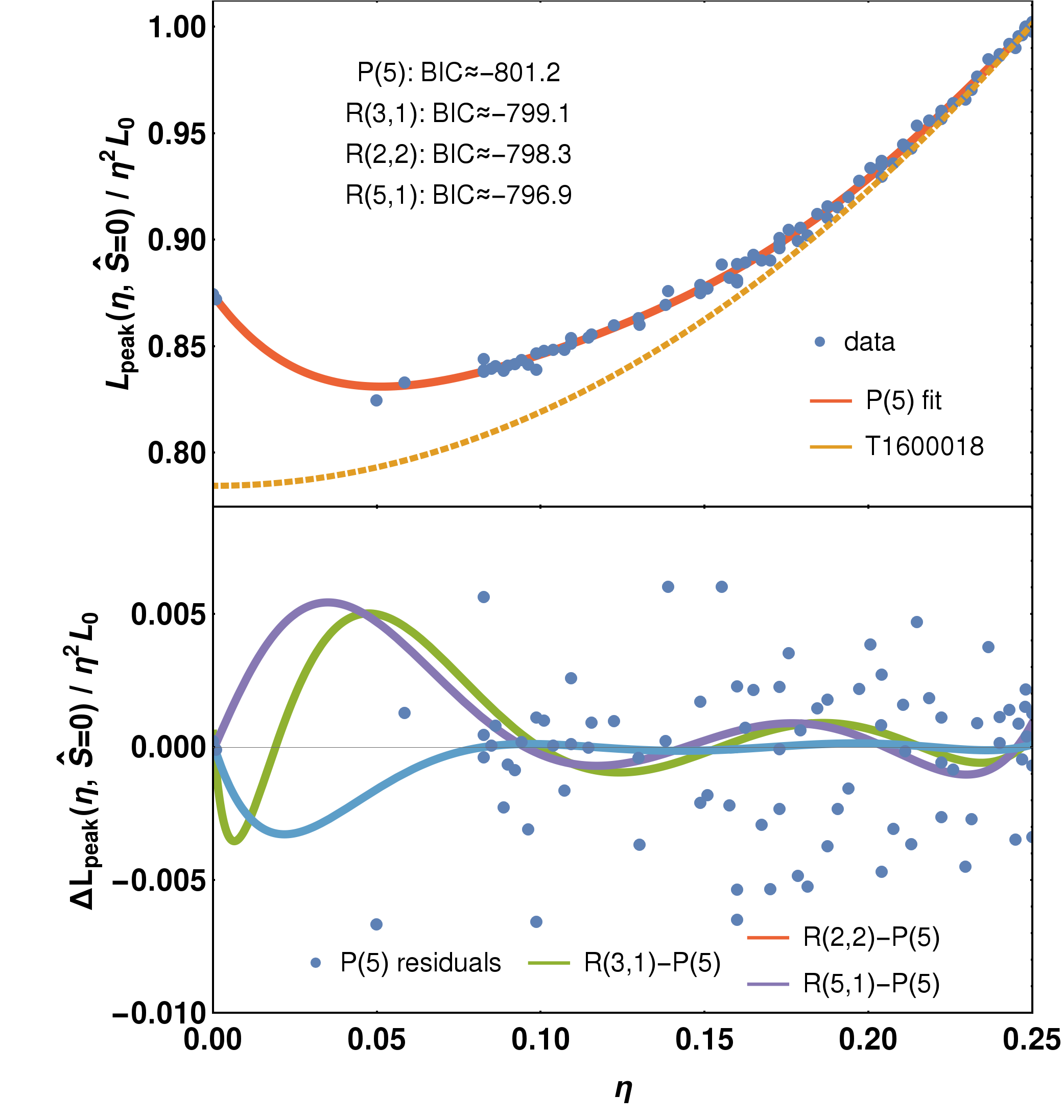
Figure 4: One-dimensional fits of the rescaled nonspinning peak luminosity $L_{\mathrm{peak}}^{\prime}\left(\eta,\widehat{S}=0\right)$. Top panel: The preferred fifth-order polynomial, see Eq. (6), and comparison with the previous fit from Ref. Jiménez Forteza et al. (2016). Lower panel: Residuals of this fit (points) and differences from the three next-highest-ranking fits in terms of BIC (lines).

	Estimate	Standard error	Relative error [$\%$]
$a_{0}$	$0.8742$	$0.0010$	$0.1$
$a_{1}$	$-2.11\hphantom{34}$	$0.28\hphantom{34}$	$13.3$
$a_{2}$	$35.2\hphantom{234}$	$7.0\hphantom{234}$	$19.9$
$a_{3}$	$-245\hphantom{.1234}$	$64\hphantom{.1234}$	$26.0$
$a_{4}$	$877\hphantom{.1234}$	$248\hphantom{.1234}$	$28.3$
$a_{5}$	$-1173\hphantom{.1234}$	$354\hphantom{.1234}$	$30.2$

Table 1: Fit coefficients for the one-dimensional non-spinning $L_{\mathrm{peak}}^{\prime}\left(\eta,\widehat{S}=0\right)$ fit over 84 data points, along with their uncertainties (standard errors) and relative errors (std.err./estimate).

With the dominant $\eta^{2}$ dependence already scaled out, fitting the higher-order corrections allows us to achieve subpercent accuracy, though the additional fit coefficients are not very tightly constrained. The top-ranked fit both by BIC and AICc (with marginally significant differences) is a fifth-order polynomial

$$L_{\mathrm{peak}}^{\prime}\left(\eta,\widehat{S}=0\right)=a_{5}\eta^{5}+a_{4}\eta^{4}+a_{3}\eta^{3}+a_{2}\eta^{2}+a_{1}\eta+a_{0}$$ ((6))

with its fit coefficients and their uncertainties given in Table 1.

Figure 1 shows this fit, its residuals and comparisons with both the previous fit from Ref. Jiménez Forteza et al. (2016) (“T1600018”) and the next-highest-ranked alternatives. These next-best alternatives are all rational functions, with the next-simpler polynomial P(4) disfavored by 7 in BIC and 20% in RMSE and the next-higher-order P(6) marginally disfavored by 4 in BIC with almost identical RMSE. We find a clear upwards correction over the T1600018 result at low $\eta$, and differences between high-ranking fits that are much smaller than this correction or the typical residuals. In the data-less region between the lowest-$\eta$ NR case ($q=18$) and the perturbative results, differences between the highest-ranking fits are larger, but still at most at the same level as the typical fit residuals at higher $\eta$, corresponding to relative errors below 0.6%. As another comparison, refitting the simple $L_{\mathrm{peak}}(\eta)=a_{2}\eta^{2}+a_{4}\eta^{4}$ ansatz that we used in Ref. Jiménez Forteza et al. (2016) (which in $L_{\mathrm{peak}}^{\prime}$ corresponds to just $\mathrm{const.}+\eta^{2}$) is disfavored by over 280 in BIC over this data set, and has a four times higher RMSE.

All highly ranked fits agree that the NR data cannot be connected to the large-mass-ratio regime with a simple monotonic function. This behavior might seem surprising, but can be explained by studying the individual modes: the observed behavior of the total peak luminosity results from competing trends of modes that either fall or rise towards $\eta\rightarrow 0$. (See Appendix A.6 and Fig. 20 for details, and Refs. Berti et al. (2007); Baker et al. (2008); Kelly et al. (2011); Pekowsky et al. (2013b); Calderón Bustillo et al. (2016) for previous studies of higher-mode amplitudes.) Also we recall that the full $L_{\mathrm{peak}}\left(\eta,\widehat{S}=0\right)$ is of course monotonic after the dominant $\eta^{2}$ term has been factored back in.

III.2 One-dimensional equal-mass-equal-spin fit

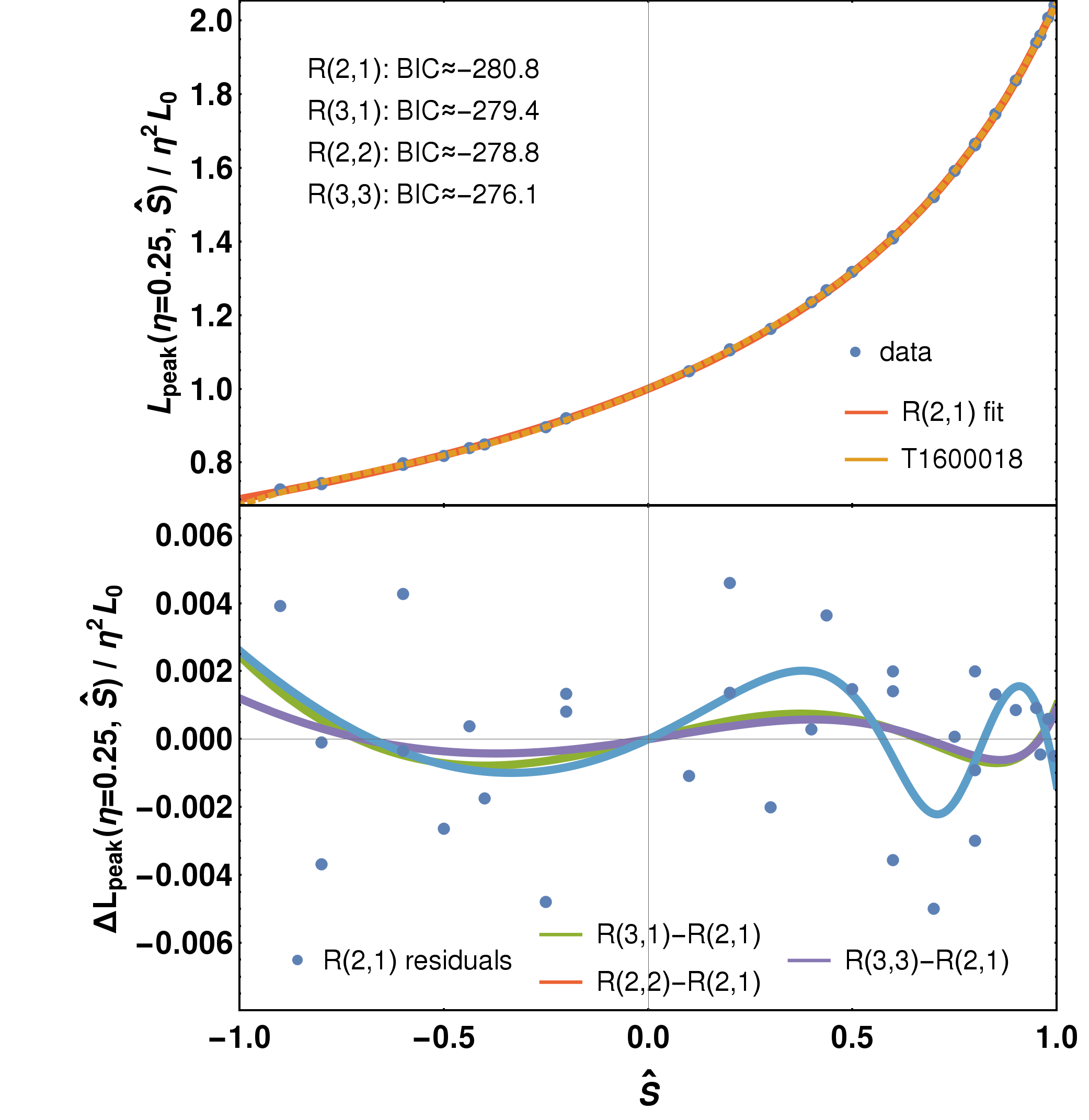
Figure 5: One-dimensional fits of the rescaled equal-mass-equal-spin ($\chi_{1}=\chi_{2}$) peak luminosity $L_{\mathrm{peak}}^{\prime}\left(\eta=0.25,\widehat{S}\right)$.
Top panel: Best fit in terms of BIC, a rational function R(2,1), see Eq. (7), and the almost indistinguishable P(5) from Ref. Jiménez Forteza et al. (2016).
Lower panel: Residuals of this fit (points) and differences from three next-best-ranked fits by BIC (lines).

	Estimate	Standard error	Relative error [$\%$]
$b_{1}$	$0.9800$	$0.0023$	$0.2$
$b_{2}$	$-0.178\hphantom{4}$	$0.028\hphantom{4}$	$15.5$
$b_{4}$	$1.786\hphantom{4}$	$0.014\hphantom{4}$	$0.6$

Table 2: Fit coefficients for the one-dimensional equal-mass-equal-spin $L_{\mathrm{peak}}^{\prime}\left(\eta=0.25,\widehat{S}\right)$ fit over 32 data points.

Next, we consider 32 equal-mass and equal-spin NR simulations, i.e. configurations with $\eta=0.25$ and $\chi_{1}=\chi_{2}\neq 0$, fitting the one-dimensional function $L_{\mathrm{peak}}^{\prime}\left(\eta=0.25,\widehat{S}\right)$. We use a similar set of polynomial and rational ansätze, with the intercept fixed by requiring consistency with the $\eta$ fit in the nonspinning case, $L_{\mathrm{peak}}^{\prime}\left(\eta=0.25,\,\widehat{S}=0\right)$. The curvature of this spin dependence at equal masses is relatively mild and can be best fit by a three-coefficient rational function ansatz

$$L_{\mathrm{peak}}^{\prime}\left(\eta=0.25,\widehat{S}\right)=\frac{0.107b_{2}\widehat{S}^{2}+0.465b_{1}\widehat{S}}{1-0.328b_{4}\widehat{S}}+1.00095\,,$$ ((7))

with the numerical prefactors being due to constructing the ansatz as a Padé approximant to simplify the handling of initial values in the fitting code. This fit is marginally top-ranked by both AICc and BIC; it is shown in Tbl. 2 and the coefficients $b_{i}$ are given in Table 2. Low-order rational functions are clearly preferred over polynomials, with the P(5) we used in Ref. Jiménez Forteza et al. (2016) disfavored by +14 in BIC and having 12% higher RMSE, and the simple R(2,1) ansatz is fully sufficient to describe the data to similar subpercent accuracy as the nonspinning set. Adding another term in either the numerator or denominator is possible, but does not improve the statistics; while adding too many terms tends to induce unconstrained coefficients or singularities within the fitting region.

III.3 Spin dependence at large mass ratios

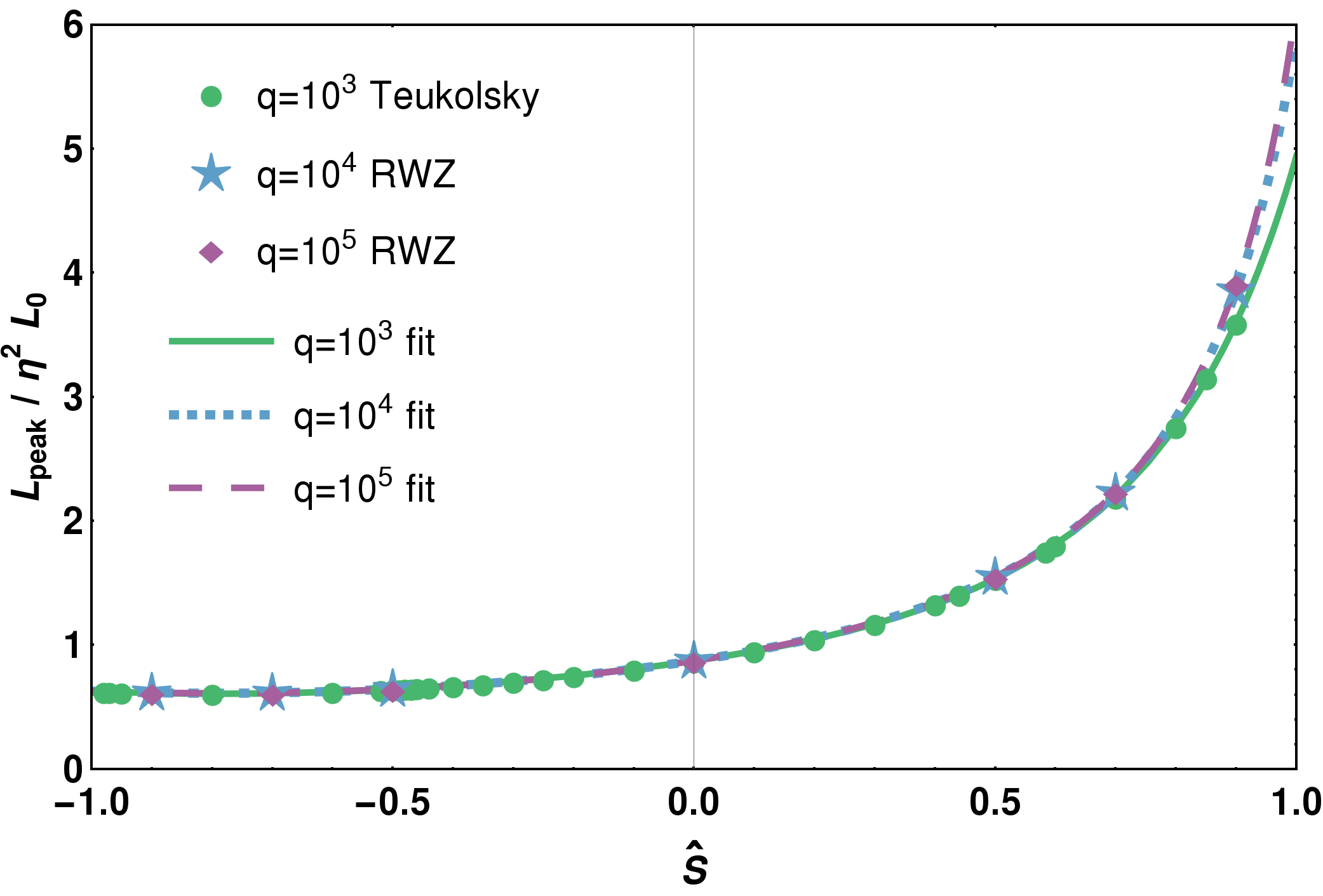
Figure 6: Numerical data from two perturbative codes (circles, stars and diamonds for mass ratios $q=\{10^{3},10^{4},10^{5}\}$), together with separate fits of the form $\mathrm{const.}+\mathrm{R}(4,1)$ at each $q$.

Analyzing the perturbative data at large mass ratios, we verify that the mass-ratio dependence is completely dominated by the leading-order $\eta^{2}$ scaling in this regime, with the rescaled $L_{\mathrm{peak}}^{\prime}$ equal to within 0.2% for the three nonspinning data points at mass ratios $q\in\left\{10^{3},10^{4},10^{5}\right\}$.

We treat the single-spin perturbative data as equivalent to results with $\chi_{1}=\chi_{2}$ which is easily accurate enough as $\widehat{S}(q=10^{3},\,\chi_{1}=1.0,\,\chi_{2}=1.0)-\widehat{S}(10^{3},1.0,0.0)\approx 10^{-6}$ and the spin-difference terms (to be fitted below in Sec. III.5) are expected to be suppressed at least by $\eta^{2}$.

We find that the spin dependence at each of these mass-ratio steps is much steeper than for equal masses, requiring a higher-order spin ansatz. A spin term at least as complex as R(4,1) is clearly preferred over any lower-order alternatives, with the $q=10^{3}$ data yielding $\Delta\mathrm{BIC}\approx 44$ and a factor $>2$ in RMSE in favor of R(4,1) against the R(2,1) found at equal masses, and similar preference even for the two highest mass ratios for which we have only seven data points available each.

Since this analysis of the large-mass-ratio data alone is only used to guide the ansatz choice in the next section, but not used directly as a constraint, we do not list the detailed results of these fits here. Instead, the final 3D fit using NR and perturbative data will be compared with the high-$q$ data in Sec. IV.2.

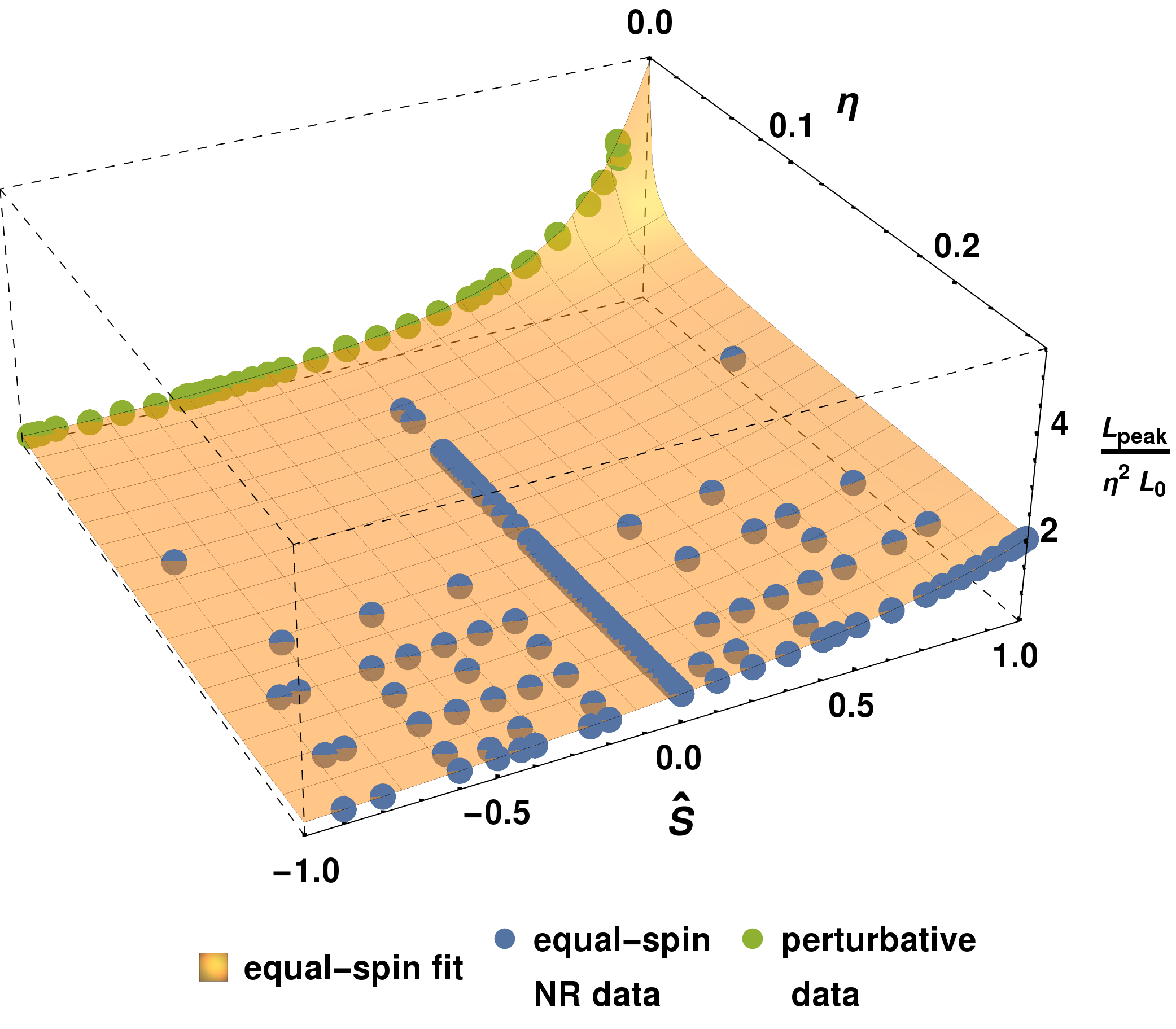
Figure 7: Results of the two-dimensional equal-spin $L_{\mathrm{peak}}^{\prime}\left(\eta,\widehat{S}\right)$ fit. First panel: Comparison of the smooth fit surface with the equal-spin NR data and perturbative results. Second panel: Residuals over the parameter space, color-coded by data provenance.

III.4 Two-dimensional fits

In proceeding with the hierarchical modeling approach, we can now make a two-dimensional (2D) equal-spin ansatz informed and constrained by the previous one-dimensional (1D) steps and the large-mass-ratio information. In Ref. Jiménez-Forteza et al. (2017), we constructed 2D final-state ansätze by first simply adding the two one-dimensional fits and then generalizing each spin coefficient by a polynomial in $\eta$. This time, we find that we need to introduce additional $\eta$-dependent higher-order terms in $\widehat{S}$, as the curvature of $L_{\mathrm{peak}}^{\prime}$ along the spin dimension increases from equal masses towards the largest mass ratios.

We thus consider a 2D ansatz of the general form

$$L_{\mathrm{peak}}^{\prime}\left(\eta,\widehat{S}\right)=L_{\mathrm{peak}}^{\prime}\left(\eta,\widehat{S}=0\right)\,+\,\mathrm{R}(m,k)\left(\eta,\widehat{S}\right)$$ ((8))

with the $\eta$ fit from Eq. (6) and the rational function $\mathrm{R}(m,k)$ in $\widehat{S}$ inheriting the coefficients $b_{i}$ from Table 2 and filled up with $b_{i}=1.0$ for orders not present in $L_{\mathrm{peak}}^{\prime}\left(\eta=0.25,\widehat{S}\right)$ from Eq. (7). We then introduce the required freedom to change the curvature along the $\eta$ dimension through the substitution

$$b_{i}\rightarrow b_{i}\sum_{j=0}^{j=J}f_{ij}\,\eta^{j}\,,$$ ((9))

with a maximum expansion order $J$.

On the other hand, the number of free coefficients is reduced again by consistency constraints with the 1D fits:

$$f_{i2} = 16 -16f_{i0}-4f_{i1}\quad\text{for }b_{i}\text{ from }\eta=0.25\text{ fit}\,,$$ ((10)a)

$$f_{i2} = -16f_{i0}-4f_{i1}\quad\text{for other }b_{i}\,.$$ ((10)b)

In practice, we use R(4,2) to match the $q=10^{3}$ result, thus introducing one extra power of $\widehat{S}$ in both the numerator and denominator compared to $L_{\mathrm{peak}}^{\prime}\left(\eta=0.25,\widehat{S}\right)$ in Eq. (7).

With 92 equal-spin data points not yet used in the two one-dimensional subspace fits (including 50 NR simulations and the single-spin large-mass-ratio results, which as discussed above can be considered as effectively equal-spin), we can easily expand the polynomials in $\eta$ from Eq. (9) to order $J=2$, $b_{i}\rightarrow b_{i}\,\left(f_{i0}+f_{i1}\eta+f_{i2}\eta^{2}\right)$, and still obtain a well-constrained fit. The only further constraint is that we set the remaining highest-order coefficient in the denominator, $f_{71}$, to zero to avoid a singularity within the physical $\left(\eta,\widehat{S}\right)$ region, leaving 11 free coefficients.

The resulting fit and its residuals over the equal-spin data set are plotted in Fig. 7. We again find subpercent relative errors over most of the calibration set, with an RMSE of $\approx 0.0057$ and only two cases over 1% relative error (both $q=8$ from BAM). There is no apparent curvature or oscillatory feature except for the large-mass-ratio region, where the $L_{\mathrm{peak}}^{\prime}$ quantity plotted in Fig. 7 overemphasizes any remaining features and the corresponding relative errors are below 0.5%. This accuracy is similar to that of the large-mass-ratio-only fits in Sec. III.3, thus proving that the combined two-dimensional fit successfully captures both the shallow spin slope at similar masses and the steep slope in the perturbative regime. As discussed in Appendix A.7, several outliers have been removed before the fit; the 2D fit still matches all equal-spin outliers to below 4% relative error.

As this equal-spin part of the full $L_{\mathrm{peak}}^{\prime}\left(\eta,\widehat{S},\Delta\chi\right)$ will be refitted, together with unequal-spin corrections, in the next and final step of the hierarchical procedure, we do not tabulate its best-fit coefficients at this point.

III.5 Unequal-spin contributions and 3D fit

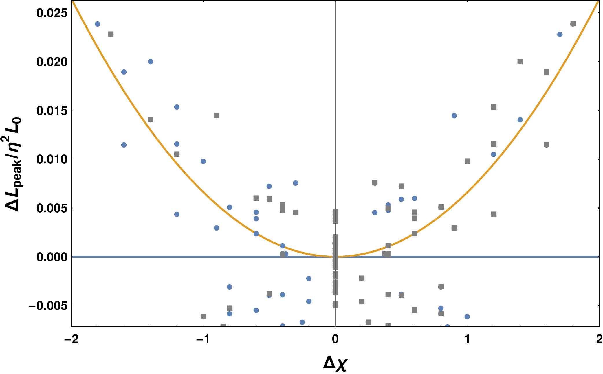
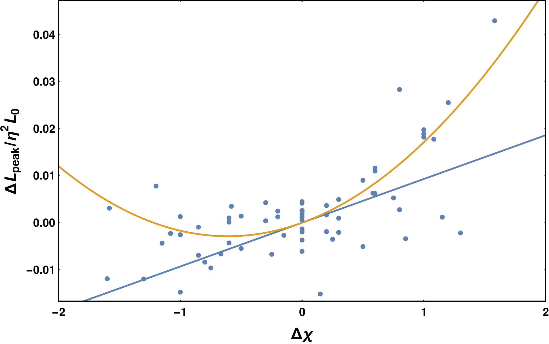
Figure 8: Examples of spin-difference behavior at fixed mass ratios, for scaled NR data $L_{\mathrm{peak}}^{\prime}$ after subtraction of the 2D $\left(\eta,\widehat{S}\right)$ fit. First panel: $q=1$ with the linear term vanishing due to symmetry and mainly quadratic dependence; points in gray are mirror duplicates exploiting the $\chi_{1}\leftrightarrow\chi_{2}$ symmetry at equal masses. There is residual scatter in the $\left|\Delta\chi\right|\lesssim 1$ range not captured by the quadratic fit, which is however not much larger than the scatter in equal-spin residuals, and hence probably related to the general uncertainties in NR data quality for $L_{\mathrm{peak}}$. Second panel: $q=3$ where the linear term dominates and the apparent quadratic dependence likely is noise dominated.

Simply extending the 2D fit to the full 3D parameter space either by evaluating fit errors of the equal-spin-only calibrated fit over the whole data set, or by refitting the 2D ansatz from Eq. (8), more than doubles the RMSE and induces oscillations at high $\left|\widehat{S}\right|$. But even for such a naive approach, relative errors are still limited to below 10%, so that the effects of unequal spins ($\chi_{1}\neq\chi_{2}$) can evidently be treated as subdominant corrections. We follow here the same approach as in Ref. Jiménez-Forteza et al. (2017) to model spin-difference effects, constructing a 3D ansatz as

$$L_{\mathrm{peak}}^{\prime}\left(\eta,\widehat{S},\Delta\chi\right)=L_{\mathrm{peak}}^{\prime}\left(\eta,\widehat{S}\right)+\Delta L_{\mathrm{peak}}^{\prime}(\eta,\widehat{S},\Delta\chi)\,.$$ ((11))

We choose the correction terms $\Delta L_{\mathrm{peak}}^{\prime}$ with guidance from (i) PN analytical results and (ii) an analysis of the residuals of unequal-spin NR simulations under the 2D equal-spin fit.

Though PN cannot be expected to be quantitatively accurate for the late-inspiral and merger stages of BBH coalescence – where the peak luminosity emanates from – it can still give some intuition on the qualitative shape of spin and spin-difference effects. The PN spin-orbit flux terms as given in Eq. (3.13) of Ref. Bohé et al. (2013) and Eq. (4.9) of Ref. Marsat et al. (2014) include linear terms in $\Delta\chi$ with an $\eta$-dependent prefactor that can be expressed as $\mathrm{P}(\eta)\sqrt{1-4\eta}$ with a polynomial $\mathrm{P}(\eta)$. The next-to-leading-order contributions would be quadratic in $\Delta\chi$ and a mixed term proportional to $\widehat{S}\Delta\chi$.

At equal masses ($\eta=0.25$) BBH configurations are symmetric under relabeling of the component BHs, so that terms linear in $\Delta\chi$ must vanish; this is ensured by the $\sqrt{1-4\eta}$ factor, which we therefore expect both in the linear and the mixture term, but not in the quadratic term. Hence, we make the general spin-difference ansatz

$$\Delta L_{\mathrm{peak}}^{\prime}\,\left(\eta,\widehat{S},\Delta\chi\right)=A_{1}(\eta)\,\Delta\chi+A_{2}(\eta)\,\Delta\chi^{2}+A_{3}(\eta)\,\widehat{S}\Delta\chi$$ ((12))

with a simple polynomial for $A_{2}(\eta)$ and $A_{1}(\eta)$, $A_{3}(\eta)$ both being a polynomial multiplied by the symmetry factor.

To check that these up to three terms accurately describe our available set of 215 unequal-spin NR cases, and to get a handle on the functions $A_{i}(\eta)$, we visually inspect the data in steps of fixed mass ratio with sufficient numbers of data points. Examples for $q=1$ and $q=3$ are shown in Fig. 8. The unequal-spin data set appears more noisy for luminosity than for the final-state quantities studied in Ref. Jiménez-Forteza et al. (2017), yet can still be analyzed following the same procedure. For each mass ratio step, $q=\{1,\,1.33,\,1.5,\,1.75,\,2,\,3,\,4,\,5,\,6,\,8\}$, we compute the residuals under the nonspinning fit from Eq. (8), then perform four fits in $\Delta\chi$: linear, linear+quadratic, linear+mixed, or the sum of all three terms. Fits of the collected coefficients, as functions of $\eta$, give estimates of the functions $A_{i}(\eta)$, as displayed with the “per-mass-ratio data” points and “per-mass-ratio fit” lines in Fig. 9.

The scatter of fit coefficients at individual mass-ratio steps is again larger than that found for final spin and radiated energy in Ref. Jiménez-Forteza et al. (2017), but this procedure still yields sufficient evidence for the existence and shape of a linear spin-difference term and some preference for including both second-order terms, though the data is too noisy to constrain their $\eta$-dependent shape very well. For example, there is an apparent sign switch in the linear term at mass ratio $q=4$ ($\eta=0.16$), which is most likely due to a combination of the 2D fit being relatively weakly constrained in this region and non-negligible errors in some of the unequal-spin data points, which however cannot easily be discarded as outliers.

The overall fits in $\eta$ are reasonably robust against such problems, and in the next step we will use not this step-by-step analysis, but a more robust fit of the full 3D ansatz to the full data set, to judge the overall significance of spin-difference terms. A full model selection of $A_{i}(\eta)$ is clearly not feasible at this point without a more detailed understanding of the point-by-point data quality. Hence, we make very simple choices for the $A_{i}(\eta)$ with just one power of $\eta$ each:

$$A_{1}(\eta) =d_{10}\sqrt{1-4\eta}\,\eta^{3}$$ ((13)a)

$$A_{2}(\eta) =d_{20}\eta^{3}$$ ((13)b)

$$A_{3}(\eta) =d_{30}\sqrt{1-4\eta}\,\eta^{3}\,,$$ ((13)c)

and investigate how much improvement this can yield over the 2D fit.

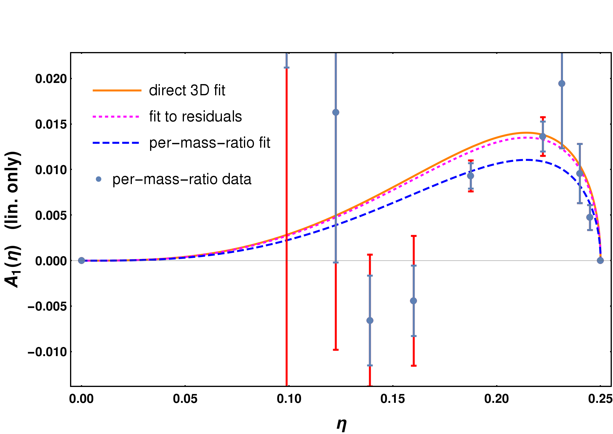
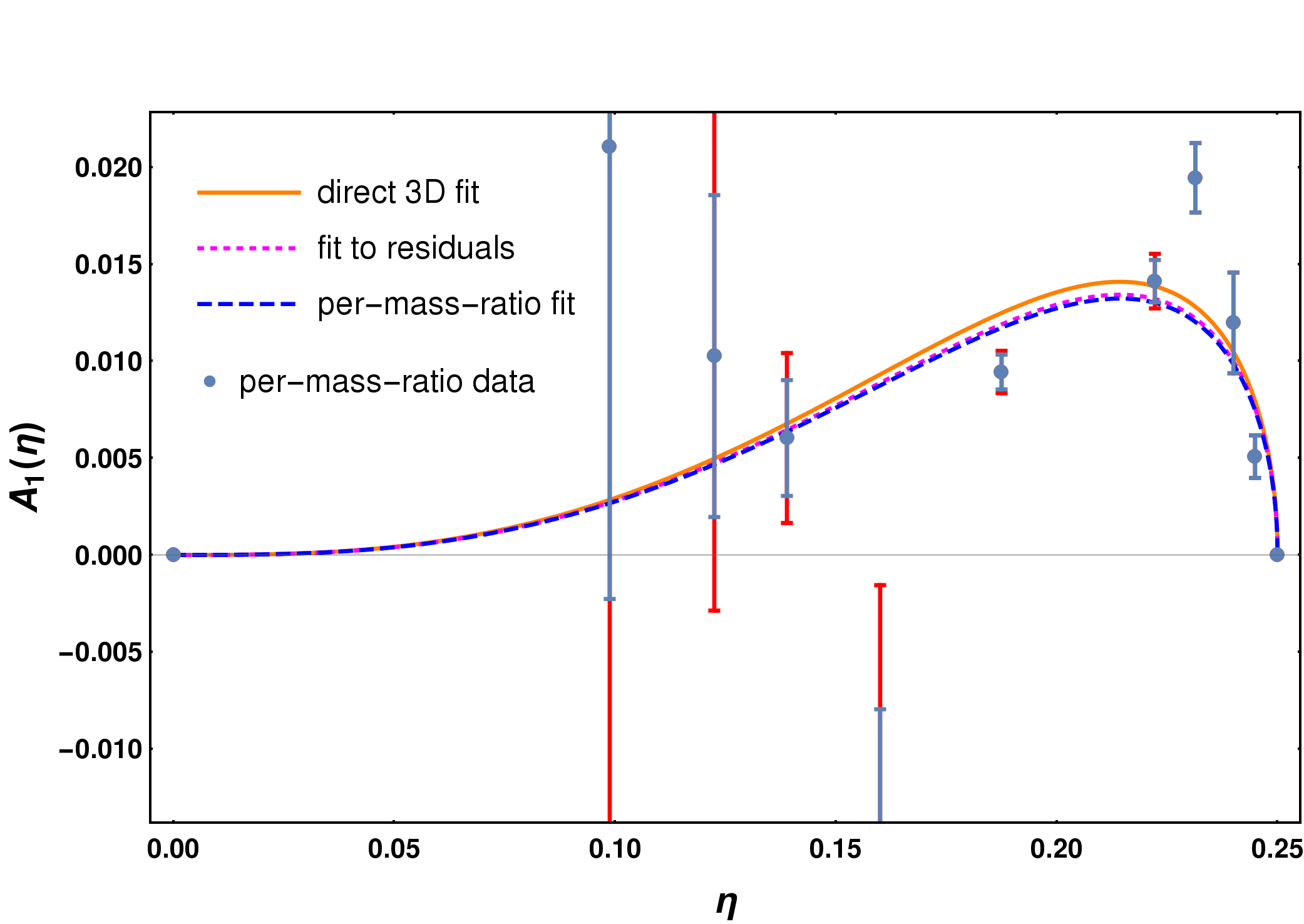
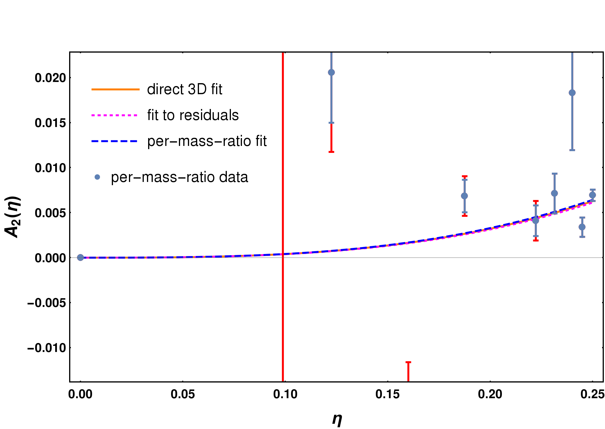
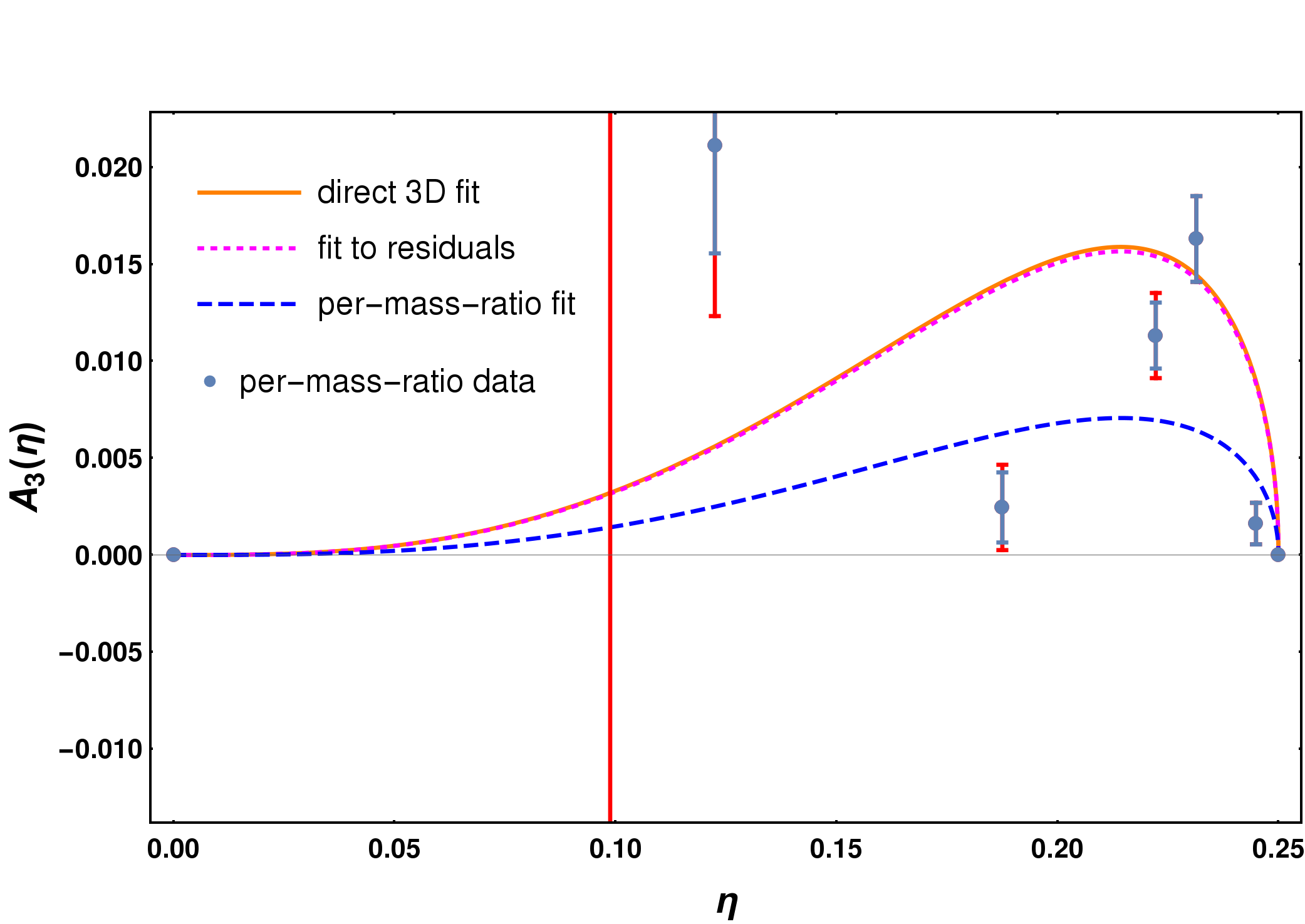
Figure 9: Spin-difference behavior of the scaled NR luminosities $L_{\mathrm{peak}}^{\prime}$ after subtraction of the 2D $\left(\eta,\widehat{S}\right)$ fit over mass ratio $\eta$, showing the results of fits as in Fig. 8 at $\eta$ steps corresponding to $q=\{1,\,1.33,\,1.5,\,1.75,\,2,\,3,\,4,\,5,\,6,\,8\}$ and three estimates for the ansatz functions $A_{i}(\eta)$ from Eq. (13): (i) unequal-spin part of the final 3D fit from Eq. (14) (“direct 3D fit”), (ii) fit of the unequal-spin terms from Eq. (13) (“fit to residuals”) to the residuals of the 2D fit from Eq. (8) over all mass ratios, and (iii) fits of Eq. (13) to the per-mass-ratio results. Top-left panel: Linear term $A_{1}$ only. The remaining panels are for the combined linear+quadratic+mixture fit, in clockwise order: linear term $A_{1}$, quadratic term $A_{2}$ and mixture term $A_{3}$. $A_{1}(\eta)$ from the combined ansatz is very similar to the linear-only fit, demonstrating its robustness. Error bars for the per-mass-ratio points include components from the fit uncertainty at that ratio (blue) and the average data weight of the contributing NR cases (red). At the lowest $\eta$, some points lie outside the plot range, but are so uncertain that they do not contribute significantly to the total fit. The direct-3D and residuals-only results are consistent, while the per-mass-ratio analysis only matches them qualitatively, which is however sufficient since it was only used to investigate the possible shapes of $A_{i}(\eta)$.

We now use the full data set except for the 1D subspaces (307 data points, including 265 NR simulations) to fit the full 3D ansatz from Eq. (11), with the equal-spin and spin-difference contributions from Eqs. (8) and (12)+(13), respectively. The sets of coefficients $a_{i}$, $b_{i}$ and $f_{i2}$ are already fixed from the 1D fits and consistency constraints (see Tables 1, 2 and Eq. (10)), leaving between 11 and 14 free coefficients in this final 3D stage. When including all three spin-difference terms, the full ansatz (with the constraints from Eq. (10) for the $f_{i2}$ still to be applied) is:

$$L_{\mathrm{peak}}^{\prime}\left(\eta,\widehat{S},\Delta\chi\right)=a_{5}\eta^{5}+a_{4}\eta^{4}+a_{3}\eta^{3}+a_{2}\eta^{2}+a_{1}\eta+a_{0}$$ ((14))

$$+\frac{0.107b_{2}\widehat{S}^{2}\left(f_{22}\eta^{2}+f_{21}\eta+f_{20}\right)+0.465b_{1}\widehat{S}\left(f_{12}\eta^{2}+f_{11}\eta+f_{10}\right)+\widehat{S}^{4}\left(f_{42}\eta^{2}+f_{41}\eta+f_{40}\right)+\widehat{S}^{3}\left(f_{32}\eta^{2}+f_{31}\eta+f_{30}\right)}{-0.328b_{4}\widehat{S}\left(f_{62}\eta^{2}+f_{61}\eta+f_{60}\right)+\widehat{S}^{2}\left(f_{72}\eta^{2}+f_{70}\right)+1.0}$$

$$+d_{20}\,\eta^{3}\left(\chi_{1}-\chi_{2}\right)^{2}+d_{10}\sqrt{1-4\eta}\,\eta^{3}\left(\chi_{1}-\chi_{2}\right)+d_{30}\sqrt{1-4\eta}\,\eta^{3}\,\widehat{S}\left(\chi_{1}-\chi_{2}\right)\,.$$

We consider residuals and information criteria, summarized in Table 3, to check which spin-difference terms are actually supported by the data. These rankings depend on the specific choice of $A_{i}(\eta)$, but with the current parameter-space coverage and understanding of NR data quality, the main goal is to find general evidence for spin-difference effects and a general idea of their shape, not to exactly characterize them. With the choices made in Eq. (13), we find a 14-coefficient fit with linear+quadratic+mixture corrections that has well-constrained coefficients (see Table 4), is evidently preferred in terms of AICc and BIC, and reduces overall residuals by about 20% in RMSE. Different choices for the powers of $\eta$ in Eq. (13) yield compatible results, while polynomials in $\eta$ with several free coefficients tend to produce underconstrained fits.

	$N_{\text{data}}$	$N_{\text{coeff}}$	RMSE	AICc	BIC
1D $\eta$	$84$	$6$	$2.81\times 10^{-3}$	$-817.1$	$-801.2$
$\text{1D }\hat{S}$	$32$	$3$	$2.42\times 10^{-3}$	$-285.8$	$-280.8$
$\left.\text{2D (}\chi_{1}=\chi_{2}\right)$	$92$	$11$	$5.65\times 10^{-3}$	$-751.7$	$-724.8$
2D all	$307$	$11$	$1.67\times 10^{-2}$	$-1914.2$	$-1870.4$
3D lin	$307$	$12$	$1.51\times 10^{-2}$	$-2008.0$	$-1960.6$
3D lin+quad	$307$	$13$	$1.39\times 10^{-2}$	$-2134.2$	$-2083.3$
3D lin+mix	$307$	$13$	$1.41\times 10^{-2}$	$-2082.6$	$-2031.7$
3D lin+quad+mix	$307$	$14$	$1.36\times 10^{-2}$	$-2157.8$	$-2103.3$

Table 3: Summary statistics for the various steps of the hierarchical fit. Note that it is not meaningful to compare AICc and BIC between data sets of different sizes. There is preference for the 3D fit including all three linear+mixture+quadratic terms, although many different choices of the $A_{i}(\eta)$ ansatz functions yield similar results with just $\pm$ a few percent in RMSE and $\pm$ a few in AICc/BIC, so that the shape of these terms is not yet strongly constrained.

	Estimate	Standard error	Relative error [$\%$]
$d_{10}$	$3.79\hphantom{3}$	$0.28\hphantom{3}$	$7.5$
$d_{20}$	$0.402$	$0.044$	$10.9$
$d_{30}$	$4.27\hphantom{3}$	$0.84\hphantom{3}$	$19.7$
$f_{10}$	$1.628$	$0.012$	$0.7$
$f_{11}$	$-3.63\hphantom{3}$	$0.23\hphantom{3}$	$6.3$
$f_{20}$	$31.7\hphantom{23}$	$1.3\hphantom{23}$	$4.2$
$f_{21}$	$-274\hphantom{.123}$	$29\hphantom{.123}$	$10.4$
$f_{30}$	$-0.235$	$0.011$	$4.7$
$f_{31}$	$6.96\hphantom{3}$	$0.44\hphantom{3}$	$6.3$
$f_{40}$	$0.211$	$0.022$	$10.6$
$f_{41}$	$1.53\hphantom{3}$	$0.45\hphantom{3}$	$29.6$
$f_{60}$	$3.090$	$0.044$	$1.4$
$f_{61}$	$-16.7\hphantom{23}$	$1.7\hphantom{23}$	$10.0$
$f_{70}$	$0.836$	$0.023$	$2.8$

Table 4: Fit coefficients for the final 3D fit stage, cf. Eq. (14).

IV Fit assessment

In this section, we assess in some detail the properties and statistical quality of the new three-dimensional peak luminosity fit, with the actual nonrescaled luminosity (in geometric units of $G=c=M=1$) obtained as $\eta^{2}\,L_{0}\,L_{\mathrm{peak}}^{\prime}\left(\eta,\widehat{S},\Delta\chi\right)$.

We compare with our previous fit Jiménez Forteza et al. (2016) used for LIGO parameter estimation during O1 Abbott et al. (2016b, c, d, e, g), which used a much smaller calibration set of 89 BAM and SXS simulations, only modes up to $\ell_{\max}=4$ and no extreme-mass-ratio constraints; and with the recent Healy&Lousto fit Healy and Lousto (2017) based on 107 RIT simulations, using modes up to $\ell_{\max}=6$. We attempt to present a fair comparison by analyzing NR and perturbative large-mass-ratio results separately, and also consider the improvement from refitting the unmodified ansätze of Refs. Jiménez Forteza et al. (2016); Healy and Lousto (2017) to the present NR data set.

IV.1 Residuals and information criteria

In Fig. 10 we show the distribution of residuals for the 3D fit in $L_{\mathrm{peak}}^{\prime}$ projected to the $\left(\eta,\widehat{S}\right)$ parameter space, so that it can be compared to the 2D results in Fig. 7. The strongest visible outliers in this scaling are at low $\eta$ and correspond to mild actual deviations; of at most a 7% relative error at $q=18$, with 417 of the 423 data points below 3% relative error.

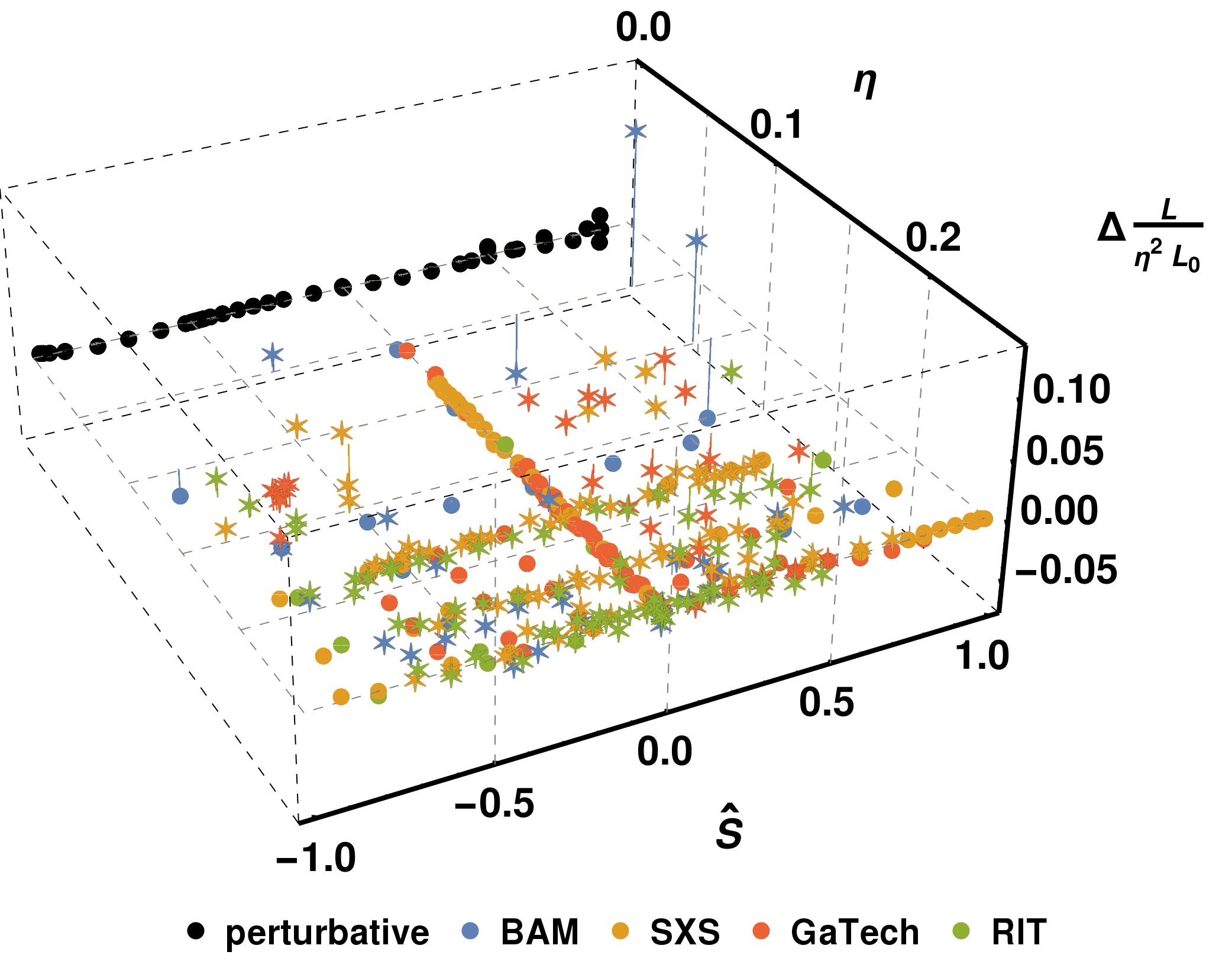
Figure 10: Residuals of the final 3D peak luminosity fit, for NR and perturbative large-mass-ratio data, projected to the 2D parameter space of $\eta$ and $\widehat{S}$. The data sets are distinguished by colors, and unequal-spin points are highlighted with stars.

For a comparison with the two previous fits, we first concentrate on the 378 NR simulations only and revisit large mass ratios in Sec. IV.2. In Tbl. 5 we show histograms of the residuals in $L_{\mathrm{peak}}$ for the three fits over this data set, demonstrating that the new fit achieves a narrower distribution. As listed in Table 5, the standard deviation of residuals is only half of that for our previous fit and three times lower than for the RIT fit. With a mean offset by only a ninth of a standard deviation, there is no evidence for bias, though that notion is notoriously ambiguous for a data set that samples the parameter space nonuniformly.

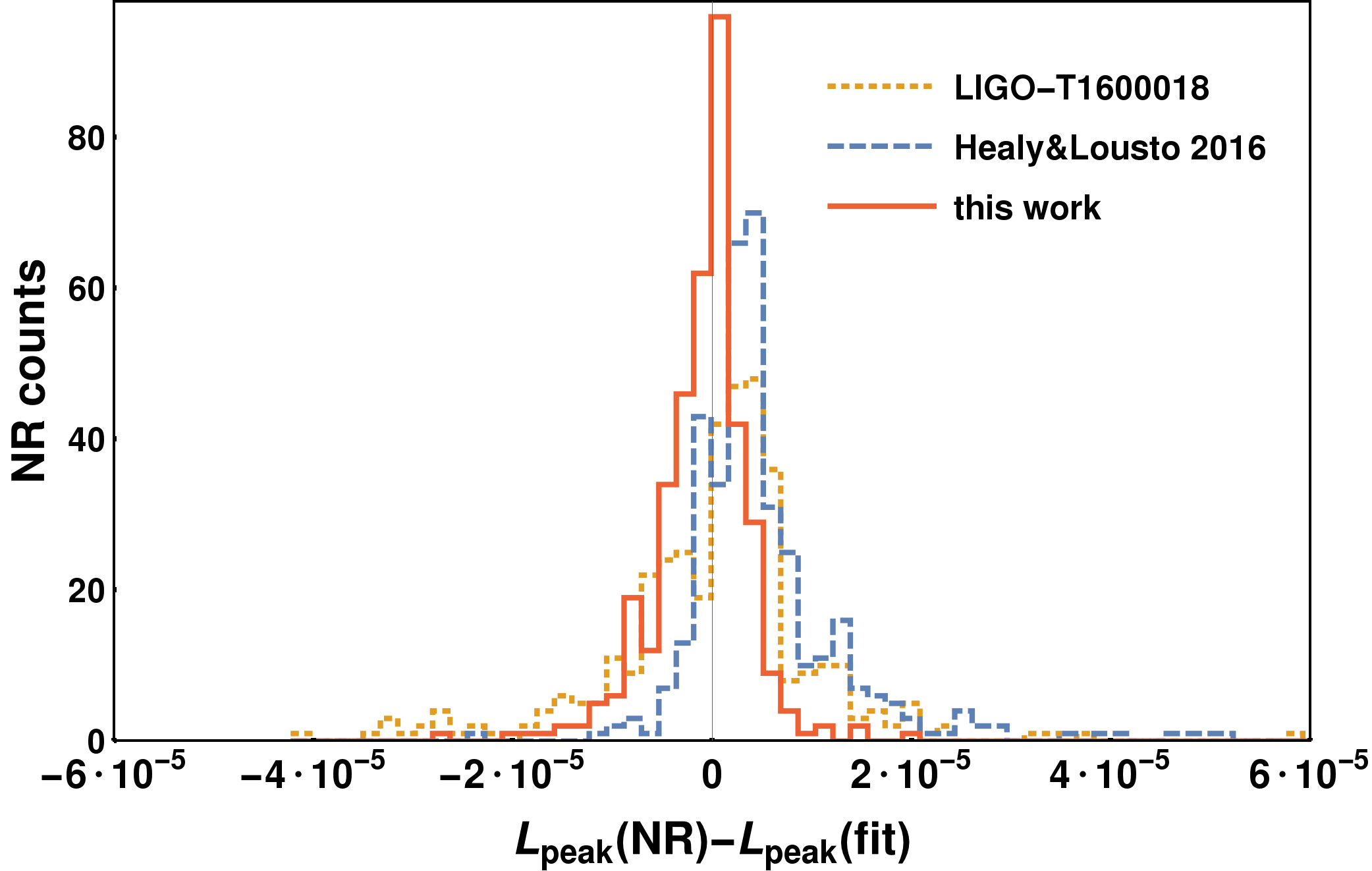
Figure 11: Fit residuals of the final 3D peak luminosity fit compared with the previous fits of LIGO-T160018 Jiménez Forteza et al. (2016) and Healy&Lousto2016 Healy and Lousto (2017), evaluated over the set of 378 NR simulations shown in Fig. 1. Six outliers for Healy&Lousto with $|\text{NR}-\text{fit}|>0.00006$ are outside of the plot range.

	$N_{\text{coef}}$	mean	stdev	AICc	BIC
T1600018	$11$	$3.0\times 10^{-7}$	$1.0\times 10^{-5}$	$-7732.1$	$-7685.6$
(refit)	$11$	$-1.8\times 10^{-6}$	$4.0\times 10^{-5}$	$-6706.0$	$-6659.5$
HL2016	$19$	$6.9\times 10^{-6}$	$1.5\times 10^{-5}$	$-7225.5$	$-7148.9$
(refit)	$19$	$-4.9\times 10^{-7}$	$1.0\times 10^{-5}$	$-7708.3$	$-7631.7$
this work	$23$	$-9.8\times 10^{-7}$	$4.8\times 10^{-6}$	$-8298.1$	$-8206.7$
(refit)	$23$	$-5.5\times 10^{-7}$	$4.8\times 10^{-6}$	$-8323.6$	$-8232.3$

Table 5: Summary statistics for the final 3D peak luminosity fit compared with previous fits with the previous fits of LIGO-T160018 Jiménez Forteza et al. (2016) and Healy&Lousto2016 Healy and Lousto (2017), evaluated over the 378 NR simulations shown in Fig. 1. The new fit has a total of 23 free coefficients, corresponding to tables 1, 2 and 4. We also show results for re-fitting the three ansätze to the full NR + large-mass-ratio data set, again evaluating the statistics over NR only.

The same table contains AICc and BIC values evaluated over the same NR-only data set, which both find a very significant preference for the new fit. Note that, being computed over a different data selection and for $L_{\mathrm{peak}}$ instead of $L_{\mathrm{peak}}^{\prime}$, these values are not directly comparable with the previous Table 3. Since we have removed 41 NR cases from the full available data set (see Appendix A.7), it is advisable to check that the statistical preference still holds when including these in the evaluation set. Indeed, the reduction in standard deviations of residuals is then less against the T1600018 and RIT fits, but still roughly 20% and 30%, and there is still a preference of several hundreds in both information criteria.

We also show results for refitting the T1600018 and RIT ansätze to the present NR + perturbative data set, with the statistics then again evaluated over NR data only. Our old ansatz with only 11 coefficients is not well suited to matching the large-mass-ratio region and the large unequal-spin population in the NR data set, and the refitted version of this 11-coefficient ansatz performs worse than the original. On the other hand, the RIT ansatz with 19 coefficients was only weakly constrained in the original version Healy and Lousto (2017) fitted to 107 simulations, with large errors on several fit coefficients, but improves now significantly through the refit. Yet, it does not achieve the same level of accuracy as the new ansatz and fit developed in this paper.

As a test of robustness, we also perform a refit of our final hierarchically obtained ansatz directly using the full data set, instead of using the constraints from the 1D subsets. This produces somewhat better summary statistics, but it also allows uncertainties from less well-controlled unequal-spin data to influence the nonspinning part of the fit. The more conservative approach is to calibrate the nonspinning part of the fit only to the corresponding data subset, as done in Sec. III.1. Hence we recommend the stepwise fit, with coefficients as reported in Tables 1, 2 and 4, for further applications.

IV.2 Large-mass-ratio and extremal-spin limits

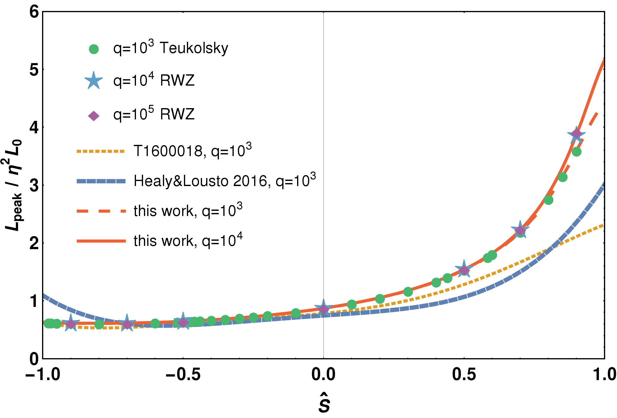
Figure 12: Full NR-calibrated fits from this work and from Refs. Jiménez Forteza et al. (2016); Healy and Lousto (2017) evaluated at large mass ratios, compared with the same perturbative data (circles, stars and diamonds for mass ratios $q=\{10^{3},10^{4},10^{5}\}$) as in Fig. 6. The T160018 and RIT fits are essentially converged at $q=10^{3}$ (e.g. 0.4% change at $S=1.0$ for the RIT fit going to $q=10^{4}$), and the visually identical lines for higher $q$ are not shown; our new fit still matches the data at higher $q$.

In Fig. 12, we compare our full 3D fit with the perturbative large-mass-ratio data and find that it correctly reproduces the behavior it is meant to be constrained to. The T1600018 fit did not predict the steep rise for positive spins, and while at negative spins it matches the shape roughly, it is still off by about 10% in that region. The RIT fit disagrees with the perturbative data at high spin magnitudes, either negative or positive, and does not reproduce the increasing steepness for even higher mass ratios.

The clearest difference between this fit and the previous ones in the NR-dominated region is for high aligned spins, which is shown in Fig. 13 for the extremal spin limit, $\chi_{1}=\chi_{2}=\widehat{S}=1$. The RIT fit estimates a lower luminosity at equal masses, but higher values at $\eta<0.16$ before approaching the $\eta\rightarrow 0$ limit rather flatly, as discussed before. Our older fit and the new one roughly agree at similar masses, but in the lower panel with the rescaled $L_{\mathrm{peak}}^{\prime}$ it is obvious that the previous fit did not anticipate the steep $\eta\rightarrow 0$ limit that we are now implementing through fitting the perturbative data.

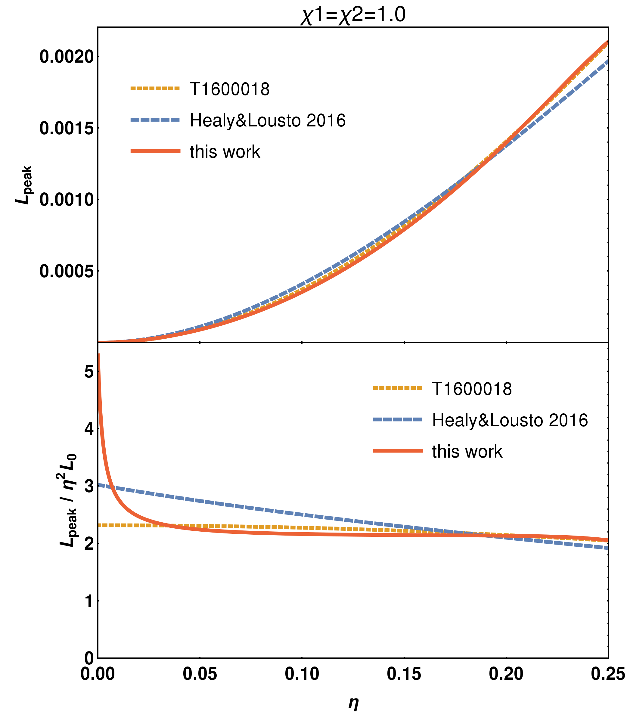
Figure 13: Behavior of the full 3D fit ((11)) in the extremal-spin limit, $\chi_{1}=\chi_{2}=\widehat{S}=1$, where there is no data available. Both panels give functions of mass ratio $\eta$, and we again compare with the fits from Refs. Jiménez Forteza et al. (2016); Healy and Lousto (2017). Top panel: In terms of physical peak luminosity $L_{\mathrm{peak}}$. Lower panel: In terms of rescaled $L_{\mathrm{peak}}^{\prime}=L_{\mathrm{peak}}/\eta^{2}L_{0}$.

V Conclusions

Using the hierarchical analysis approach to the three-dimensional parameter space of nonprecessing quasicircular binary black hole (BBH) coalescences introduced in Ref. Jiménez-Forteza et al. (2017), we have developed a new model for the peak of the gravitational-wave luminosity of BBH coalescence events, $L_{\mathrm{peak}}$. This model fit is based on the largest-yet combined set of numerical relativity (NR) results from four independent simulation codes, as well as on perturbative numerical data for the large-mass-ratio regime not currently probed by NR.

The result that BBHs are, for a brief moment during their merger, the most powerful astrophysical events is already clear from dimensional analysis and simplified order-of-magnitude estimates, as is the rough scaling of this peak luminosity with mass ratio. Yet, only detailed NR-calibrated fits allow for a precise understanding of the parameter-space dependence of $L_{\mathrm{peak}}$. Our new fit significantly reduces the residuals for most available NR cases in comparison with a previous version of this fitting procedure Jiménez Forteza et al. (2016) used in LIGO O1 data analysis and an alternative fit Healy and Lousto (2017), both calibrated to much smaller data sets.

We also characterized the quality of the luminosity data set considering various sources of NR inaccuracies and the compatibility between different simulation codes, finding that the peak luminosity’s subdominant parameter dependencies are of a similar or even smaller order than typical discrepancies between simulations. This limits the level of detail to which we can model spin-difference effects, though we can still improve over an equal-spin-only fit ($\chi_{1}=\chi_{2}$) and find that the spin-difference dependence qualitatively matches expectations. These statistical improvements, wider parameter-space coverage and systematic understanding of sources of uncertainty can make the new fit a useful ingredient for future parameter estimation studies of BBH events.

The final fit ansatz is given in Eq. (14), with coefficient estimates listed in Tables 1, 2 and 4. Example implementations of this fit for Mathematica and python are available as Supplementary Material Keitel et al. (2017a); *Keitel:2016krm-anc, along with an ASCII table of the data set. The python implementation is equivalent to that included in the free software LALInference LIGO Scientific Collaboration package.

As more GW detections are made, there will be more opportunities to infer the luminosities of stellar-mass BBH systems. In particular, the aLIGO observatories in the USA Aasi et al. (2015); Abbott et al. (2016a), Advanced Virgo Acernese et al. (2015) in Italy, and forthcoming observatories in Japan Somiya (2012); Aso et al. (2013) and India Unnikrishnan (2013) are poised to become pivotal tools for earth-based GW astronomy, eventually enabling daily BBH detections Aasi et al. (2016) over a wide parameter range.

The accuracy of the fit presented in this paper should be sufficient for the expected sensitivity at least during the second aLIGO observing run and for “vanilla” BBH events (similar masses, low spins, no strong precession), with sampling uncertainties in mass ratio and spins still dominating over fit errors. Still, a continued expansion of the NR calibration set and an improved understanding of higher-mode contributions, precession and the transition from similar-mass to extreme-mass-ratio regimes will be important to improve the understanding of BBH peak luminosities and waveforms.

Meanwhile, this project of fitting peak luminosities is an important step in extending the “Phenom” waveform family Husa et al. (2016); Khan et al. (2016); Hannam et al. (2014); Bohé et al. (2016, ), as our analysis of higher-mode contributions and the demonstration of joint calibration to NR and perturbative large-mass-ratio data can form the basis for improved modeling of full inspiral-merger-ringdown waveforms.

Appendix A NR data investigations

As a first estimate of the overall accuracy of the peak luminosity data set, we study the differences between results from different codes for equal initial parameters. We then give additional details on the possible error sources listed in Sec. II.1 and on the properties of higher modes, and discuss the 41 cases not used in the calibration set.

A.1 Comparison between different codes

To analyze typical deviations between results from different NR codes, we identify simulations with initial BH parameters equal to within numerical accuracy, with a tolerance criterion

$$\left|\lambda_{i}-\lambda_{j}\right|\leq\epsilon=0.0002\;\text{for}\;\lambda_{i}=\left\{\eta_{i},\,\chi_{1i},\,\chi_{2i}\right\}\,.$$ ((15))

This threshold was found in Appendix A of Ref. Jiménez-Forteza et al. (2017) to be strict enough to reliably identify equivalent initial configurations, and is also tolerant enough to accommodate the minor relaxation of parameters after the initial “junk” radiation which may be different between codes. In Fig. 14 we show the relative difference in $L_{\mathrm{peak}}$ between such matching cases, including the nonspinning $q=4$ case where we have results from all four codes and a few triple coincidences. The set of these tuples is too sparse for clear conclusions on the parameter-space dependence of discrepancies between codes, though there might be some indication of increasing differences at large positive spins, which are particularly challenging to simulate due to increased resolution requirements for capturing the larger metric gradients in the near-horizon zone. We find many pairs with differences below 1%, but also several up to a few % even at not particularly challenging configurations.

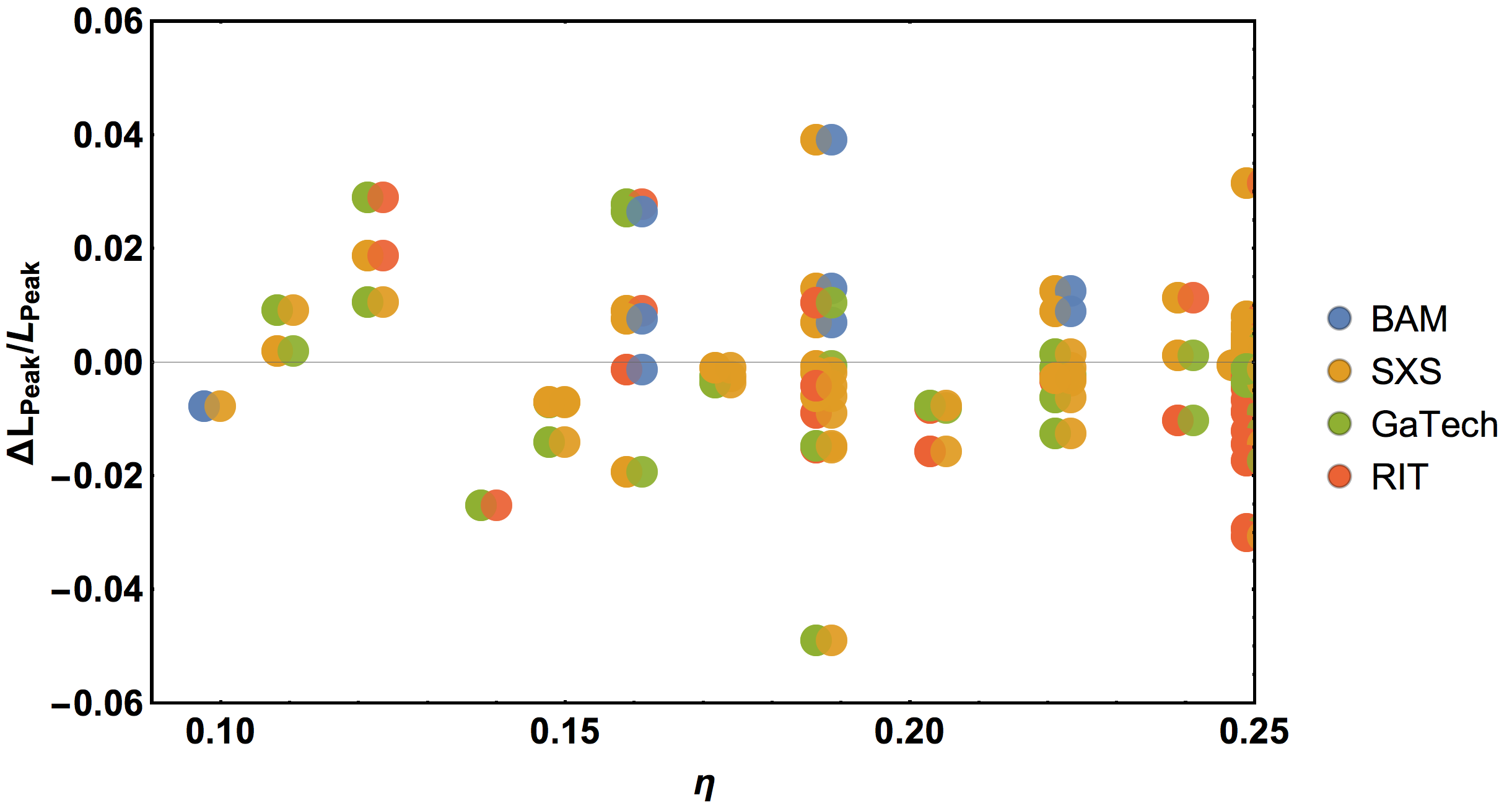
Figure 14: Relative differences in the peak luminosity for equal-parameter configurations from different NR codes, shown against the symmetric mass ratio $\eta$. Pairs of simulations are shown with a small horizontal offset for ease of visual identification.

This study gives a useful overall estimate of the possible error magnitude on the NR data set: while certainly many simulations are accurate to more than the few-% level, in general for any given simulation that does not have a paired case from another code, or at least nearby neighbors in parameter space, we cannot confidently assume that the errors will be low. This affects in particular the unequal-spin cases, where due to the much larger 3D parameter space very few duplicates exist. On the other hand, for equal spins – and particularly for the densely covered nonspinning or equal-mass subsets – we can use the duplicates analysis to make a very strict selection of calibration points, allowing the subpercent calibration demonstrated in Secs. III.1 and III.2. The specific decisions are detailed below in Appendix A.7.

As shown in the histograms of Fig. 15, the overall distribution of (relative) differences between equivalent configurations is of a similar width than that of the fit residuals. This demonstrates that we are indeed not overfitting the data, but also that one would need to characterize the accuracy of all NR cases to a significantly lower level to extract more information on subdominant effects.

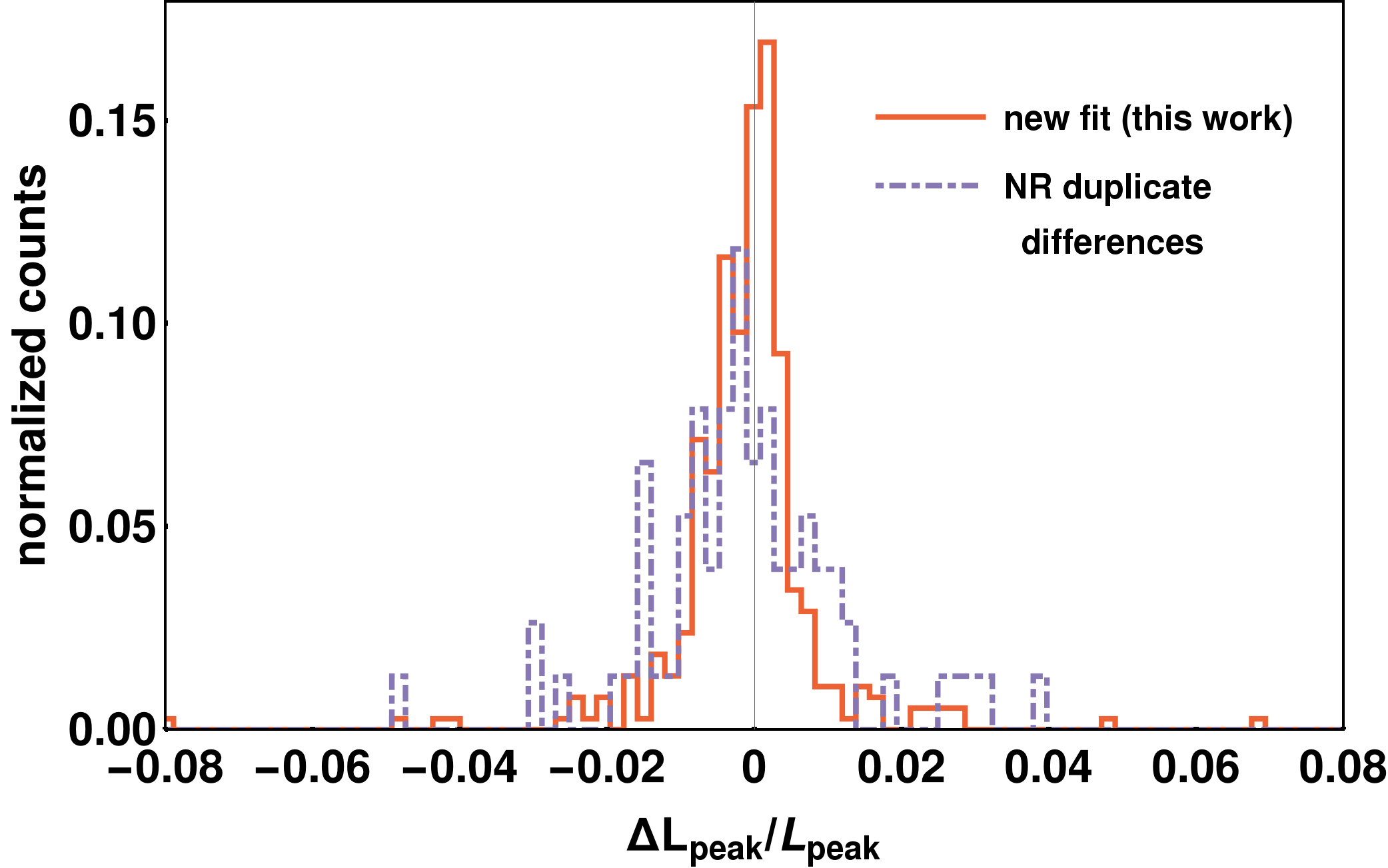
Figure 15: Comparison of the distribution of relative fit errors (NR only, same set as in Tbl. 5) and of differences between NR codes for equivalent parameters.

A.2 Luminosity computation from $\psi_{4}$

Equations ((1)) and ((2)) describe the general computation of peak luminosities from the Weyl curvature component $\psi_{4}(t,\vec{r})$. This conversion is normally performed by either integrating $\psi_{4}(t,\vec{r})$ twice in time or by first applying a Fourier transform to the data, both to finally obtain the strain $h(t)$. However, both strategies for computing $h(t)$ carry the same technical issue: nonlinear drifts in the final strain as a consequence of the characteristic low-frequency noise present when operating on finite segments of data.

This problem was already solved in Ref. Reisswig and Pollney (2011) by means of the FFI algorithm, which we briefly describe here. One takes the Fourier-domain strain as

$$\widetilde{h}\,(f)=\begin{cases}-\frac{\widetilde{\psi_{4}}(f)}{f^{2}},&\text{if}\quad f\geq f_{0}\,,\\ \\ -\frac{\widetilde{\psi_{4}}(f)}{f_{0}^{2}},&\text{if}\quad f<f_{0}\,.\end{cases}$$ ((16))

All physical frequency content must be contained in $\left[f_{0},f_{\mathrm{QNM}}\right]$ where $f_{0}$ must be tuned close to the lowest physical frequency for a given mode and $f_{\mathrm{QNM}}$ is the quasinormal mode frequency of the same mode. Thus, a proper selection of $f_{0}$ down-weights contributions from the low-frequency regime, driving these effects to zero – see Fig. 16.

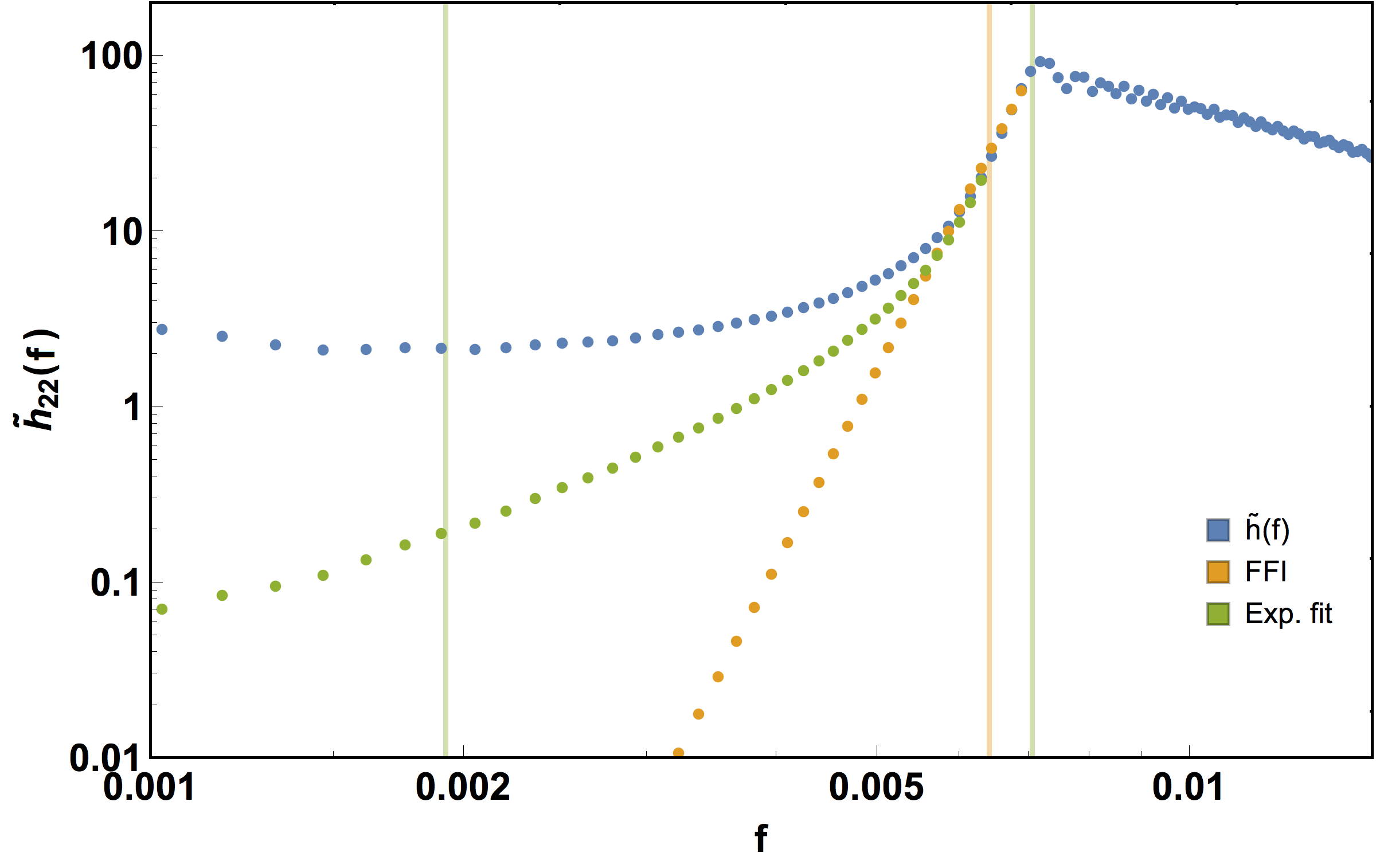
Figure 16: Comparison of the FFI algorithm and the exponential-fit method for the low-frequency regime of $\widetilde{h}_{22}(f)$, for the example of the $q=10$ nonspinning SXS waveform “SXS:BBH:0185”. The green vertical lines indicate the local maximum and minimum of $\widetilde{h}_{22}(f)$ and the yellow line is at the tuned value $f_{0}$ for the FFI.

As a consistency check, we have developed an alternative conversion from $\psi_{4}(t)$ to $h(t)$ which avoids the step of tuning $f_{0}$. In Fig. 16 we show an example of the Fourier transform $\widetilde{h}_{22}(f)$ of the dominant-mode strain. In general, both local maxima and minima are located in the $\left[f_{\min}\sim 0.5f_{0},f_{\max}\sim 1.2f_{0}\right]$ range. The plotted low-frequency behavior occurs for any $\widetilde{h}_{22}(f)$ independently of the system’s physical parameters, as a consequence of the finiteness and discreteness of the time-domain waveforms. Empirically we found that the data in $\left[f_{\min},f_{\max}\right]$ can be well fit with an exponential ansatz, which is then extended to all data in $\left[0,f_{\max}\right]$ and combined with the original data above $f_{\max}$:

$$\widetilde{h}_{\ell m}(f)=\begin{cases}-\frac{\widetilde{\psi}_{4,\ell m}(f)}{f^{2}},&\text{if }f\geq f_{\max}\,,\\ a\exp^{-(b-f)}f^{c}\mathrm{e}^{i\phi_{\ell m}},&\text{if }f<f_{\max}\,,\end{cases}$$ ((17))

where $\phi_{\ell m}$ is the original $\psi_{4}$ phase. The split in the fit coefficients $a$ (amplitude) and $b$ (peak position) is introduced here so that good starting values for the fit function can be picked more easily. With this approach, we smoothly drive the low-frequency noise to zero, eliminating nonphysical artifacts in the Fourier-domain data.

We find that the difference between peak luminosities from the two different algorithms, when $f_{0}$ is optimally selected, is generally negligible, e.g. it is about $\sim 0.05\%$ in the example of the $q=10$ nonspinning SXS waveform, and no significantly larger discrepancies have been found over the data set. So this effect is negligible for our analysis in comparison with other sources of uncertainty.

A.3 Extrapolation

The NR waveforms used in this paper are extracted at finite radii, which implies ambiguities, in particular due to gauge effects. We therefore extrapolate all waveforms to null infinity, where unambiguous waveforms can be defined. This allows us to assemble a consistent set of peak luminosity values for different codes, and to estimate the errors due to finite radius effects.

However, the extraction properties of the codes are not equal, and thus we have extrapolated the available waveforms following the following prescriptions.

1. BAM: We have calculated $L_{\mathrm{peak}}$ at each finite radius and then performed a linear-in-$1/R$ extrapolation using only the well-resolved extraction radii. The maximum used for any case is $R\leq 180M$, but for some cases significantly fewer radii can be used for a robust extrapolation, depending on simulation grid resolutions.

2. GaTech: $L_{\mathrm{peak}}$ is again calculated at finite radii and then extrapolated with a fit quadratic in $1/R$, only using up to $R\leq 100M$ because the slope generally changes for higher radii; this choice of extrapolation order and radius cut yields the most consistent results with other codes in the analysis of equivalent configurations.

3. SXS: These waveforms are already provided at second-, third- and fourth-order polynomial extrapolation, and we compute $L_{\mathrm{peak}}$ from these data products, after a correction Boyle (2013); Boyle et al. (2014); Boyle (2016) for center-of-mass drift, using the 2nd order extrapolation as the preferred value following Refs. Boyle et al. (2007); Calderón Bustillo et al. (2015). We use waveforms based on the Weyl scalar $\psi_{4}$, but also compare with waveforms based on a computation of the strain. The SXS $\psi_{4}$ data use a definition of null-tetrad which is different from their Regge-Wheeler-Zerilli strain data Regge and Wheeler (1957); Zerilli (1970); Sarbach and Tiglio (2001); Rinne et al. (2009), and from the definition used in other codes. For the luminosity this difference corresponds to an overall scaling factor of the lapse function to the fourth power as a consequence of the difference between Eqs. (30)–(33) in Ref. Bruegmann et al. (2008) and Eqs. (11)–(12) in Ref. Boyle et al. (2007). A rough correction for the different tetrad scaling used to compute the Weyl scalar $\psi_{4}$ is to multiply it by $\alpha^{4}$ with $\alpha=1-2M_{\mathrm{f}}/R$, where $M_{\mathrm{f}}$ is the final mass and $R$ is an approximation to the luminosity distance using the standard relation with the isotropic radial coordinate for the Schwarzschild spacetime. (Compare also with the analysis in Ref. Nakano et al. (2015).) Comparisons of SXS luminosities computed from $\psi_{4}$, strain, and heuristically rescaled $\psi_{4}$ with data from other codes are included in Figs. 18 and 18.

4. RIT: The luminosity data provided in Ref. Healy and Lousto (2017) uses the extrapolation method of Ref. Nakano et al. (2015).

In Fig. 18 we show the only configuration, the nonspinning $q=4$ case, for which we have data from all four codes. This includes peak luminosities computed from the finite-radius strain data available as additional data products from SXS to cross-check the pre-extrapolated value. We see that extrapolation for $R\rightarrow\infty$ reduces discrepancies in $L_{\mathrm{peak}}$ between the different codes, but cannot completely alleviate it in this case. Another similar example is shown in Fig. 18 for a $q=2.5$ nonspinning configuration where we have three simulations from SXS, GaTech and RIT, with the GaTech and RIT values being more consistent with each other than with SXS in this case.

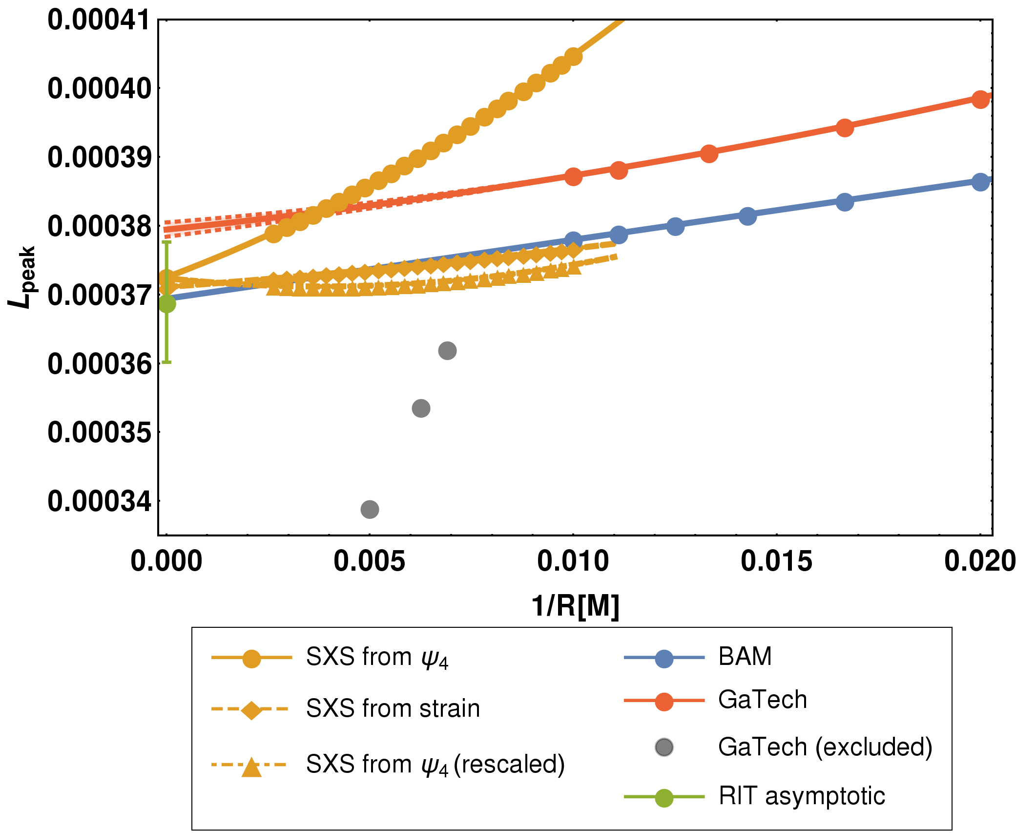
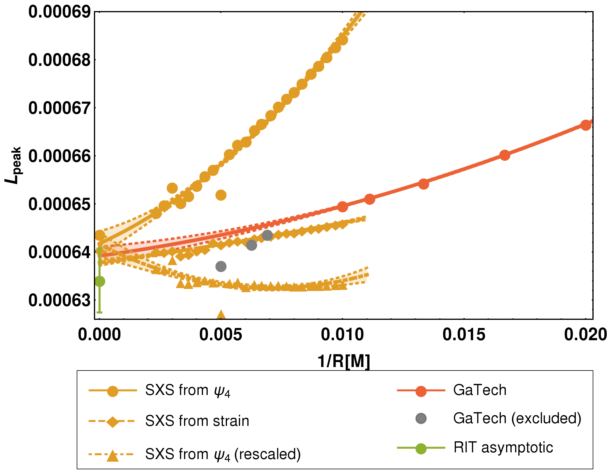
Figure 17: $q=4$ nonspinning example of extrapolation from finite radii for BAM, SXS and GaTech, with second-order fits for SXS and GaTech and linear for BAM; as well as the RIT value extrapolated with the method of Ref. Nakano et al. (2015) and its error bar also containing a finite-resolution estimate. In this case we find consistent values from BAM, SXS and RIT, with the GaTech case being an outlier. The $R>100$M GaTech data would make the trend more inconsistent, and are excluded from extrapolation. SXS luminosities computed from strain, or from $\psi_{4}$ but with the $\alpha^{4}$ rescaling discussed in the text, show a flatter finite-$R$ behavior more similar to the other codes, and extrapolated values consistent with the luminosity from $\psi_{4}$.

Figure 18: $q=2.5$ nonspinning example of extrapolation behavior for SXS and GaTech, compared with the extrapolated RIT value. In this case we find consistent GaTech and RIT values, with the asymptotic SXS computed from $\psi_{4}$ a marginal outlier. Extrapolating the finite-radius peak luminosities computed from $\psi_{4}$ with rescaling, or from strain, seems to improve consistency in this example, which however needs further study before applying it to the whole data set.

The uncertainties of extrapolation fits for BAM, SXS and GaTech can be estimated by the standard deviation on the intersection parameter (equivalent to the confidence interval on the extrapolation to $1/R=0$). For the plotted nonspinning $q=4$ case, these are smaller than the remaining largest difference between the results from GaTech and other codes, while for $q=2.5$ the uncertainties are almost wide enough to make the results marginally consistent. For some other cases, these uncertainties can reach up to a few %, especially when we want to be conservative and take the maximum of (i) the statistical uncertainty for the standard extrapolation-order choice and (ii) the difference between this and the closest alternative order. In general, such an uncertainty estimate cannot provide information about any systematics present in the data from different codes, and indeed for example we find that for BAM the purely statistical extrapolation uncertainties are much smaller in some high-$q$ cases than for low-$q$ cases which are generally considered more reliable.

Hence, a study of the extrapolation uncertainties over the whole parameter space is useful in gaining an understanding of the properties of the different codes, but cannot directly be used as a measure of total NR uncertainties.

A.4 Finite resolution

The error contribution from finite numerical resolution can be estimated through convergence tests, reproducing the same configuration at different resolutions. This multiplies computational cost and is hence only practical for a small set of representative simulations. Comparisons of NR results at different resolutions have been discussed e.g. in Refs. Husa et al. (2008, 2016) for the BAM code and in Ref. Lovelace et al. (2016) for GW150914-like SXS and RIT waveforms. For peak luminosities specifically, multiresolution results are available for some BAM and RIT simulations.

The error estimates presented for 107 RIT simulations in Tables XI–XIII of Ref. Healy and Lousto (2017) combine finite-resolution and finite-radius contributions, but for four cases at mass ratios $q\approx\{1,1.33,2,3\}$ and different spins we can extract error estimates due to finite resolution only from Tables XIV–XVII, by comparing $L_{\mathrm{peak}}$ extrapolated to $r_{\mathrm{obs}}=\infty$ for the highest finite resolution with $L_{\mathrm{peak}}$ extrapolated to both infinite radius and infinite resolution. This yields relative error estimates $\Delta L_{\mathrm{peak}}/L_{\mathrm{peak}}$ of about 0.8–1.6%.

These estimates fall well within the distributions of our fit residuals and of the ”duplicates“ study, as shown in Fig. 15, and from comparison with the combined RIT error estimates and with Appendix A.3 on extrapolation from finite extraction radius we also see that these two error contributions are typically on a comparable level.

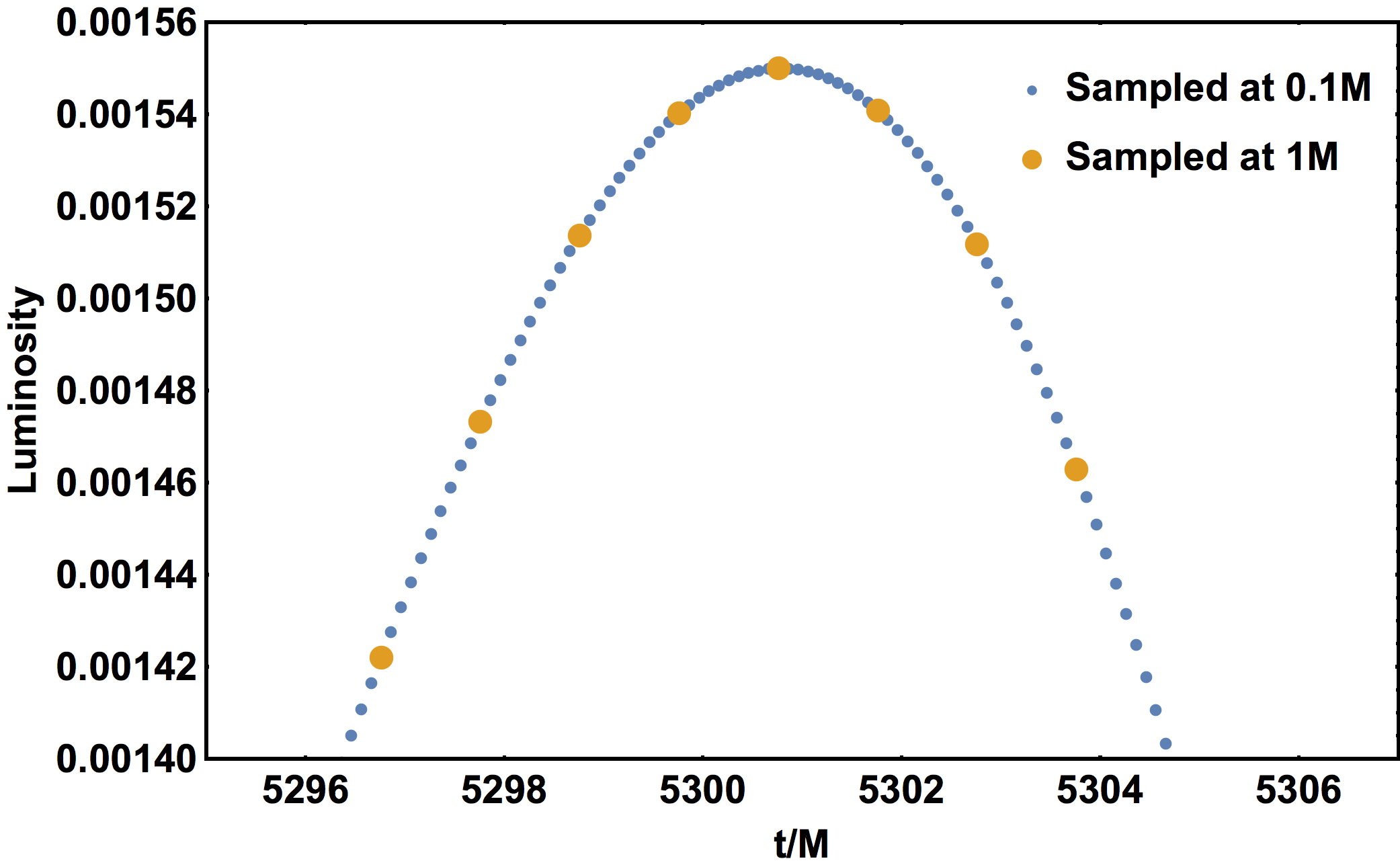
Figure 19: Luminosity computed with different sampling rates in time, for the nonspinning $q=10$ SXS waveform “SXS:BBH:0185” or “BBH_CFMS_d11d2_q10_sA_0_0_0_sB_0_0_0”.

Convergence testing for BAM runs at the particularly challenging $q=18$ mass ratio has previously been discussed in Husa et al. (2016), indicating generally robust behavior. Estimating the finite-difference error as the difference between the highest resolution and a Richardson extrapolation yields $<1\%$ for both $\psi_{4}$ and $L_{\mathrm{peak}}$ in the nonspinning $q=18$ case, and for the $\chi_{1}=0.4$ simulation we find $\approx 1\%$ for $\psi_{4}$ and $\approx 4\%$ for $L_{\mathrm{peak}}$. We already knew that these simulations at high mass ratios must have wider overall error bars due to e.g. the higher-mode contributions.

Hence, finite resolution can be conjectured to be a nondominant, but also non-negligible contribution to the total uncertainty budget, while a point-by-point evaluation is hindered by the large computational cost.

A.5 Peak accuracy

Since we are dealing with discrete numerical data sets, the peak finding might also be a problem if the sampling is not fine enough; particularly for high mass-ratio cases where the higher modes become more relevant and it is important to sample each mode accurately so that the overall peak profile is not washed out. We have estimated this contribution to NR uncertainties by applying two different time samplings to the data: for the actual $L_{\mathrm{peak}}$ values used in this paper, we use $\Delta t=0.1M$, while here we compare also with a coarser $\Delta t=1M$ to illustrate the possible loss of accuracy.

In Fig. 19 we show, for an SXS mass-ratio 10 nonspinning case, that the uncertainty contribution, measured as the difference between two points bracketing the peak, would be about 1% of the total peak luminosity with the coarser sampling, but is only about 0.05% for the finer sampling that we actually use. As a worst case, we found 0.2% for the nonspinning $q=18$ BAM result.

A.6 Mode selection

As introduced in Eq. (2), we compute NR peak luminosities for BAM, SXS and GaTech waveforms as sums over all modes up to $\ell_{\max}=6$. The RIT luminosities from Refs. Healy et al. (2014); Healy and Lousto (2017) use the same cutoff. For the perturbative data from Refs. Nagar et al. (2007); Bernuzzi et al. (2011a); Harms et al. (2014) at large mass ratios, we use $\ell_{\max}=8$. These choices are based on studying the individual contribution of each mode to the total luminosity, finding that $\ell>6$ contributions are sufficiently small to be discarded for the NR data in comparison with other sources of uncertainty.

As an illustrative example, we show in the top panel of Fig. 20 the cumulative peak luminosity when adding modes $\ell$ by $\ell$ (including all $|m|\leq\ell$ at each step) for the $q=10$ nonspinning SXS waveform, and the per-$\ell$ contributions in the lower panel. The falloff of the higher-$\ell$ contributions to the global peak is expected to be exponential, which is indeed found in this case.

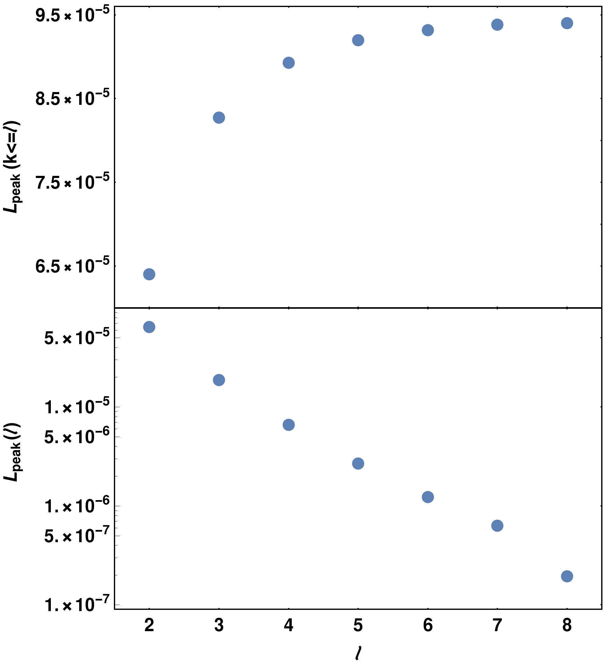
Figure 20: Per-mode contributions to the total peak luminosity for the same SXS case as in Fig. 19. Top panel: Cumulative sum up to $\ell$. Lower panel: Natural logarithm of the luminosity contribution per $\ell$. Each point contains all $m$ for the given $\ell$. Similar behavior for large mass ratios was found in Ref. Bernuzzi et al. (2011b).

To quantify and extrapolate the loss generally expected for nonspinning configurations, we have estimated the relative loss in $L_{\mathrm{peak}}$ from not including the $\ell=7,8$ modes for nonspinning SXS waveforms up to mass ratio $q=10$ (maximum loss of 0.6%) and the nonspinning BAM simulation at $q=18$ (loss of 1%), and fit a quadratic function in $\eta$:

$$\frac{\Delta L_{\mathrm{peak}}}{L_{\mathrm{peak}}}=0.017611-0.153760\eta+0.334803\eta^{2}\,.$$ ((18))

This result is illustrated in Fig. 22, together with a marginally consistent fit when including the $q=10^{3}$ Teukolsky result (loss of 2%). The $\ell>6$ contributions are smaller for negative spins and larger for positive spins, as illustrated in the same figure with $\chi_{1}=\pm 0.8$ results at $q=10^{3}$ and from BAM at $q=18$. The largest loss for any NR case investigated is $\lesssim 2$% for the $q=18$, $\chi_{1}=+0.8$ BAM case, which is a significant contribution to the overall error budget but still on the level of other error sources. For the perturbative large-mass-ratio results, with a worst-case $\ell>6$ of $\approx 5$%, we use $\ell_{\max}=8$ instead, so that the loss from $\ell>8$ is limited to $<1$%.

Figure 21: Relative loss in the peak luminosity including modes up to $\ell_{\max}=6$ against $\ell_{\max}=8$, for nonspinning SXS cases up to $q=10$, a nonspinning BAM case with $q=18$ and the $q=10^{3}$ Teukolsky result. Also shown are $q=18$ and $q=10^{3}$ results for $\chi_{1}=+0.8$ (above the nonspinning line) and for $\chi_{1}=-0.8$ (below), as well as the quadratic nonspinning fit from Eq. (18) to NR data points only and a fit of the same order including the $q=10^{3}$ point, with 90% confidence intervals for both fits.

Figure 22: Comparison of rescaled peak luminosities for nonspinning SXS and BAM and perturbative large-mass-ratio data, for a small selection of modes. The points for each mode have been scaled by the maximum for that mode, which is at $\eta=0.25$ for the 22 mode and at $\eta\rightarrow 0$ for the other modes. The connecting lines are fifth-order polynomial fits, which were not statistically optimized and just added to guide the reader’s eye. This can be compared with the sum over modes in Tbl. 1. As a guide to the overall strength of the individual modes, we list the nonrescaled maxima $\max_{\eta}L_{\mathrm{peak}}^{\ell m}(\widehat{S}=0)$ of each of the displayed modes $(\ell m)=\{22,33,44,55,21,20\}$: $\{1.0\times 10^{-3},5.9\times 10^{-5},1.5\times 10^{-5},5.3\times 10^{-6},9.8\times 10^{-6},6.3\times 10^{-7}\}$.

	q	$\chi_{1}$	$\chi_{2}$	$L_{\text{peak}}$	$\text{$\Delta$L}_{\text{peak}}$	$\text{$\Delta$L}_{\text{peak}}/L_{\text{peak}}$	tag	code
$1$	$1.00$	$0.20$	$0.80$	$0.00133540$	$-0.00001456$	$-0.011$	Q1.00$\_$0.20$\_$0.80	RIT
$2$	$1.00$	$0.25$	$0.25$	$0.00114910$	$-0.00001078$	$-0.009$	Q1.0000$\_$0.2500$\_$0.2500	RIT
$3$	$1.00$	$0.40$	$0.80$	$0.00143030$	$-0.00001617$	$-0.011$	Q1.00$\_$0.40$\_$0.80	RIT
$4$	$1.00$	$0.50$	$0.50$	$0.00132610$	$-0.00002155$	$-0.016$	Q1.0000$\_$0.5000$\_$0.5000	RIT
$5$	$1.00$	$0.80$	$0.80$	$0.00165190$	$-0.00005163$	$-0.031$	Q1.0000$\_$0.8000$\_$0.8000	RIT
$6$	$1.00$	$0.97$	$0.97$	$0.00185963$	$-0.00017055$	$-0.092$	d15$\_$q1$\_$sA$\_$0$\_$0$\_$0.97$\_$sB$\_$0$\_$0$\_$0.97$\_$ecc6e-4	SXS
$7$	$1.00$	$-0.80$	$-0.80$	$0.00075683$	$-0.00000522$	$-0.007$	d15$\_$q1$\_$sA$\_$0$\_$0$\_$-0.8$\_$sB$\_$0$\_$0$\_$-0.8	SXS
$8$	$1.00$	$-0.95$	$-0.95$	$0.00071785$	$-0.00001083$	$-0.015$	d15$\_$q1$\_$sA$\_$0$\_$0$\_$-0.95$\_$sB$\_$0$\_$0$\_$-0.95	SXS
$9$	$1.10$	$0.00$	$0.00$	$0.00102562$	$0.00000646$	$0.006$	D9$\_$q1.1$\_$a0.0$\_$m160	GaT
$10$	$1.33$	$0.50$	$0.50$	$0.00127610$	$-0.00001496$	$-0.012$	Q0.7500$\_$0.5000$\_$0.5000	RIT
$11$	$1.33$	$0.80$	$-0.80$	$0.00113510$	$0.00001336$	$0.012$	Q0.7500$\_$-0.8000$\_$0.8000	RIT
$12$	$1.33$	$0.60$	$0.80$	$0.00144390$	$-0.00002266$	$-0.016$	Q1.33$\_$0.80$\_$0.60	RIT
$13$	$1.50$	$0.00$	$0.00$	$0.00092086$	$-0.00000929$	$-0.010$	Q0.6667$\_$0.0000$\_$0.0000	RIT
$14$	$1.67$	$0.00$	$0.00$	$0.00089059$	$0.00001118$	$0.013$	Q0.6000$\_$0.0000$\_$0.0000	RIT
$15$	$2.00$	$0.85$	$-0.85$	$0.00104805$	$-0.00005372$	$-0.051$	q2$\_$-85$\_$85$\_$0.2833$\_$it2$\_$T$\_$96$\_$468	BAM
$16$	$2.00$	$0.60$	$0.60$	$0.00113005$	$-0.00001154$	$-0.010$	D11$\_$q2.00$\_$a0.60$\_$m200	GaT
$17$	$2.00$	$0.85$	$0.00$	$0.00119969$	$-0.00004465$	$-0.037$	q2$\_$0$\_$85$\_$0.566667$\_$T$\_$80$\_$360	BAM
$18$	$2.00$	$0.80$	$0.80$	$0.00133220$	$-0.00004371$	$-0.033$	Q2.00$\_$0.80$\_$0.80	RIT
$19$	$2.00$	$0.60$	$0.50$	$0.00109870$	$-0.00002568$	$-0.023$	Q0.5000$\_$0.5000$\_$0.6000	RIT
$20$	$2.00$	$0.80$	$0.00$	$0.00115110$	$-0.00004828$	$-0.042$	Q0.5000$\_$0.0000$\_$0.8000	RIT
$21$	$2.50$	$0.00$	$0.00$	$0.00064369$	$0.00000637$	$0.010$	BBH$\_$CFMS$\_$d16.9$\_$q2.50$\_$sA$\_$0$\_$0$\_$0$\_$sB$\_$0$\_$0$\_$0	SXS
$22$	$3.00$	$0.50$	$-0.50$	$0.00067168$	$-0.00002270$	$-0.034$	q3$\_$-50$\_$50$\_$0.25$\_$T$\_$80$\_$400	BAM
$23$	$3.00$	$0.00$	$0.00$	$0.00051866$	$-0.00000761$	$-0.015$	D10$\_$q3.00$\_$a0.0$\_$0.0$\_$m240	GaT
$24$	$3.00$	$0.40$	$0.00$	$0.00065030$	$-0.00001591$	$-0.024$	D10$\_$q3.00$\_$a0.4$\_$0.0$\_$m240	GaT
$25$	$3.00$	$0.50$	$0.80$	$0.00074376$	$-0.00001267$	$-0.017$	Q0.3333$\_$0.8000$\_$0.5000	RIT
$26$	$3.00$	$0.60$	$0.00$	$0.00074392$	$-0.00003003$	$-0.040$	D10$\_$q3.00$\_$a0.6$\_$0.0$\_$m240	GaT
$27$	$3.00$	$0.67$	$0.00$	$0.00078909$	$-0.00002904$	$-0.037$	Q3.00$\_$0.00$\_$0.67	RIT
$28$	$3.00$	$0.80$	$-0.80$	$0.00084159$	$-0.00002278$	$-0.027$	Q3.00$\_$-0.80$\_$0.80	RIT
$29$	$3.00$	$0.85$	$0.85$	$0.00107685$	$0.00003335$	$0.031$	BBH$\_$SKS$\_$d13.9$\_$q3$\_$sA$\_$0$\_$0$\_$0.850$\_$sB$\_$0$\_$0$\_$0.850	SXS
$30$	$4.00$	$0.75$	$0.75$	$0.00069840$	$0.00001188$	$0.017$	q4a075$\_$T$\_$112$\_$448	BAM
$31$	$4.00$	$0.75$	$0.00$	$0.00063280$	$-0.00002841$	$-0.045$	Q4.00$\_$0.00$\_$0.75	RIT
$32$	$4.00$	$0.00$	$0.00$	$0.00037948$	$0.00000782$	$0.021$	D10$\_$q4.00$\_$a0.0$\_$0.0$\_$m240	GaT
$33$	$4.30$	$0.00$	$0.00$	$0.00034217$	$0.00000421$	$0.012$	D9$\_$q4.3$\_$a0.0$\_$m160	GaT
$34$	$4.50$	$0.00$	$0.00$	$0.00031462$	$-0.00000329$	$-0.010$	D9$\_$q4.5$\_$a0.0$\_$m160	GaT
$35$	$5.00$	$0.80$	$0.00$	$0.00052483$	$-0.00000926$	$-0.018$	Q5.00$\_$0.00$\_$0.80	RIT
$36$	$5.00$	$0.00$	$0.00$	$0.00026999$	$-0.00000480$	$-0.018$	D10$\_$q5.00$\_$a0.0$\_$0.0$\_$m240	GaT
$37$	$5.00$	$0.40$	$0.00$	$0.00034792$	$-0.00001784$	$-0.051$	D10$\_$q5.00$\_$a0.4$\_$0.0$\_$m240	GaT
$38$	$6.00$	$0.00$	$0.00$	$0.00020707$	$-0.00000395$	$-0.019$	Q0.1667$\_$0.0000$\_$0.0000	RIT
$39$	$6.00$	$0.00$	$0.00$	$0.00021325$	$0.00000234$	$0.011$	D10$\_$q6.00$\_$a0.00$\_$0.00$\_$m280	GaT
$40$	$6.00$	$0.20$	$0.00$	$0.00023419$	$-0.00000829$	$-0.035$	D10$\_$q6.00$\_$a0.20$\_$0.00$\_$m280	GaT
$41$	$18.00$	$-0.80$	$0.00$	$0.00006179$	$0.00003868$	$0.626$	q18a0aM08c025$\_$96$\_$fine	BAM

Table 6: NR cases from the source catalogs not included in the fit calibration, for reasons detailed in the text.

Another useful investigation is to consider the $\eta$ dependence, and especially the $\eta\rightarrow 0$ behavior, for individual modes. Fitting $L_{\mathrm{peak}}^{\prime}\left(\eta,\widehat{S}=0\right)$ in Sec. III.1 we found, as illustrated in Tbl. 1, that the peak luminosity of all modes summed up to $\ell_{\max}=6$, after scaling out the dominant $\eta^{2}$ dependence, is not a monotonic function towards low $\eta$. The increasing relative amplitudes of higher-order modes at low $\eta$ have been studied with NR results previously Berti et al. (2007); Baker et al. (2008); Kelly et al. (2011); Pekowsky et al. (2013b); Calderón Bustillo et al. (2016), but with our large peak luminosity data set we can now investigate the slope more closely.

Repeating the same comparison as in Tbl. 1 of rescaled nonspinning peak luminosities between NR (SXS+BAM nonspinning) and perturbative large-mass-ratio data, but for individual modes, we find – as shown in Fig. 22 for a subset of modes – that these are all monotonic as $\eta\rightarrow 0$; however, the slopes are very different, with the dominant 22 mode falling off faster than $\eta^{2}$ and the subdominant and higher modes falling off much slower, consistent with the general expectation of stronger contributions at low $\eta$. This finding of monotonicity in each mode increases our trust in the combination of NR and perturbative results, and the nonmonotonicity of the rescaled peak luminosities after summing the modes can thus be explained as a superposition of these counteracting trends in the individual modes.

A.7 Cases not used in fit calibration

Of the full catalog of 419 NR simulations from four codes, we have only used 378 to calibrate our new fit. Of the 41 removed cases, 22 are non-spinning or equal-spin configurations. Of these, 17 belong to one of the pairs or groups of equivalent initial parameters identified in Appendix A.1, with differences between the paired results inconsistent at a level higher than the fit residuals we can otherwise achieve in the corresponding subspace fit; or they are individual points inconsistent with an otherwise consistent set of direct neighbors. In these cases we removed from each tuple the case most discrepant with the others and with the global trend. This includes for example the GaTech $q=4$ and SXS $q=2.5$ nonspinning cases shown in the extrapolation comparisons of Figs. 18 and 18, or the SXS $\left(q=1,\widehat{S}=0.97\right)$ point whose luminosity seems inconsistent with other $q=1$, high-spin SXS results.

We emphasize that in the one-dimensional fits for nonspinning and equal-mass-equal-spin BBHs we calibrate the fits to subpercent accuracies, so that this is a very strict criterion for removing cases, which mainly serves to guarantee a very clean calibration of the well-covered subspaces and dominant effects so that in the later steps we have a better chance of isolating and extracting subdominant effects from the general, more noisy data set. In terms of total absolute or relative errors compared with the whole NR data set, several of these cases are not overly inaccurate, and we do not imply that necessarily there are data quality issues with the waveforms from which the luminosities are calculated.

The remaining cases were identified as strong outliers outside of the main distribution in the visual inspection of the two-dimensional equal-spin fit (Sec. III.4) and the per-mass-ratio analysis of residuals of unequal-spin cases against the 2D fit (Sec. III.5). For these simulations, there are no equivalent or nearby comparison cases, so it cannot be said with certainty whether they would still be outliers in a more densely covered future data set; and at the same time a small residual for any given point is no guarantee for its absolute accuracy when there are no equivalent comparison points. Hence, we have made much less strict exclusions in the sparsely covered unequal-spin range, which limits the accuracy to which we can extract the subdominant spin-difference effects (which are of a similar scale as the remaining scatter in the data set), but also reduces the risk of overfitting to spurious trends in a more strongly trimmed data set.

References

- Aasi et al. (2015) J. Aasi et al. (LIGO Scientific Collaboration), Class. Quant. Grav. 32, 074001 (2015), arXiv:1411.4547 [gr-qc] .
- Abbott et al. (2016a) B. P. Abbott et al. (LIGO Scientific Collaboration and Virgo Collaboration), Phys. Rev. Lett. 116, 131103 (2016a), arXiv:1602.03838 [gr-qc] .
- Abbott et al. (2016b) B. P. Abbott et al. (LIGO Scientific Collaboration and Virgo Collaboration), Phys. Rev. Lett. 116, 061102 (2016b), arXiv:1602.03837 [gr-qc] .
- Abbott et al. (2016c) B. P. Abbott et al. (LIGO Scientific Collaboration and Virgo Collaboration), Phys. Rev. Lett. 116, 241103 (2016c), arXiv:1606.04855 [gr-qc] .
- Abbott et al. (2016d) B. P. Abbott et al. (LIGO Scientific Collaboration and Virgo Collaboration), Phys. Rev. X6, 041015 (2016d), arXiv:1606.04856 [gr-qc] .
- Abbott et al. (2016e) B. P. Abbott et al. (LIGO Scientific Collaboration and Virgo Collaboration), Phys. Rev. Lett. 116, 241102 (2016e), arXiv:1602.03840 [gr-qc] .
- Abbott et al. (2016f) B. P. Abbott et al. (LIGO Scientific Collaboration and Virgo Collaboration), Phys. Rev. Lett. 116, 221101 (2016f), arXiv:1602.03841 [gr-qc] .
- Frederiks et al. (2013) D. D. Frederiks et al., Astrophys. J. 779, 151 (2013), arXiv:1311.5734 [astro-ph.HE] .
- Jiménez Forteza et al. (2016) X. Jiménez Forteza, D. Keitel, S. Husa, M. Hannam, S. Khan, L. London, and M. Pürrer, Phenomenological fit of the peak luminosity from non-precessing binary-black-hole coalescences, Tech. Rep. LIGO-T1600018-v4 (2016).
- Aasi et al. (2013) J. Aasi et al. (LIGO Scientific Collaboration and Virgo Collaboration), Phys. Rev. D88, 062001 (2013), arXiv:1304.1775 [gr-qc] .
- Veitch et al. (2015) J. Veitch, V. Raymond, B. Farr, W. Farr, P. Graff, S. Vitale, B. Aylott, K. Blackburn, N. Christensen, M. Coughlin, W. Del Pozzo, F. Feroz, J. Gair, C.-J. Haster, V. Kalogera, T. Littenberg, I. Mandel, R. O’Shaughnessy, M. Pitkin, C. Rodriguez, C. Röver, T. Sidery, R. Smith, M. Van Der Sluys, A. Vecchio, W. Vousden, and L. Wade, Phys. Rev. D91, 042003 (2015), arXiv:1409.7215 [gr-qc] .
- Abbott et al. (2016g) B. Abbott et al. (LIGO Scientific Collaboration and Virgo Collaboration), Phys. Rev. X6, 041014 (2016g), arXiv:1606.01210 [gr-qc] .
- Hannam et al. (2014) M. Hannam, P. Schmidt, A. Bohé, L. Haegel, S. Husa, F. Ohme, G. Pratten, and M. Pürrer, Phys. Rev. Lett. 113, 151101 (2014), arXiv:1308.3271 [gr-qc] .
- Bohé et al. (2016) A. Bohé, M. Hannam, S. Husa, F. Ohme, M. Pürrer, and P. Schmidt, PhenomPv2 – technical notes for the LAL implementation, Tech. Rep. LIGO-T1500602 (2016).
- (15) A. Bohé, M. Pürrer, M. Hannam, S. Husa, F. Ohme, P. Schmidt, et al., “IMRPhenomPv2 publication,” in preparation.
- Husa et al. (2016) S. Husa, S. Khan, M. Hannam, M. Pürrer, F. Ohme, X. Jiménez Forteza, and A. Bohé, Phys. Rev. D93, 044006 (2016), arXiv:1508.07250 [gr-qc] .
- Khan et al. (2016) S. Khan, S. Husa, M. Hannam, F. Ohme, M. Pürrer, X. Jiménez Forteza, and A. Bohé, Phys. Rev. D93, 044007 (2016), arXiv:1508.07253 [gr-qc] .
- Pan et al. (2014) Y. Pan, A. Buonanno, A. Taracchini, L. E. Kidder, A. H. Mroué, H. P. Pfeiffer, M. A. Scheel, and B. Szilágyi, Phys. Rev. D89, 084006 (2014), arXiv:1307.6232 [gr-qc] .
- Pürrer (2014) M. Pürrer, Class. Quant. Grav. 31, 195010 (2014), arXiv:1402.4146 [gr-qc] .
- Pürrer (2016) M. Pürrer, Phys. Rev. D93, 064041 (2016), arXiv:1512.02248 [gr-qc] .
- Babak et al. (2017) S. Babak, A. Taracchini, and A. Buonanno, Phys. Rev. D95, 024010 (2017), arXiv:1607.05661 [gr-qc] .
- Abbott et al. (2017) B. P. Abbott et al. (LIGO Scientific Collaboration and Virgo Collaboration), Class. Quant. Grav. 34, 104002 (2017), arXiv:1611.07531 [gr-qc] .
- Healy et al. (2014) J. Healy, C. O. Lousto, and Y. Zlochower, Phys. Rev. D90, 104004 (2014), arXiv:1406.7295 [gr-qc] .
- Healy and Lousto (2017) J. Healy and C. O. Lousto, Phys. Rev. D95, 024037 (2017), arXiv:1610.09713 [gr-qc] .
- Hofmann et al. (2016) F. Hofmann, E. Barausse, and L. Rezzolla, Astrophys. J. 825, L19 (2016), arXiv:1605.01938 [gr-qc] .
- Jiménez-Forteza et al. (2017) X. Jiménez-Forteza, D. Keitel, S. Husa, M. Hannam, S. Khan, and M. Pürrer, Phys. Rev. D95, 064024 (2017), arXiv:1611.00332 [gr-qc] .
- Baker et al. (2008) J. G. Baker, W. D. Boggs, J. Centrella, B. J. Kelly, S. T. McWilliams, and J. R. van Meter, Phys. Rev. D78, 044046 (2008), arXiv:0805.1428 [gr-qc] .
- Nagar et al. (2007) A. Nagar, T. Damour, and A. Tartaglia, Class. Quant. Grav. 24, S109 (2007), arXiv:gr-qc/0612096 [gr-qc] .
- Bernuzzi et al. (2011a) S. Bernuzzi, A. Nagar, and A. Zenginoğlu, Phys. Rev. D84, 084026 (2011a), arXiv:1107.5402 [gr-qc] .
- Harms et al. (2014) E. Harms, S. Bernuzzi, A. Nagar, and A. Zenginoğlu, Class. Quant. Grav. 31, 245004 (2014), arXiv:1406.5983 [gr-qc] .
- Amaro Seoane et al. (2013a) P. Amaro Seoane et al., GW Notes 6, 4 (2013a), arXiv:1201.3621 [astro-ph.CO] .
- Amaro Seoane et al. (2013b) P. Amaro Seoane et al. (eLISA Consortium), (2013b), arXiv:1305.5720 [astro-ph.CO] .
- Klein et al. (2016) A. Klein, E. Barausse, A. Sesana, A. Petiteau, E. Berti, S. Babak, J. Gair, S. Aoudia, I. Hinder, F. Ohme, and B. Wardell, Phys. Rev. D93, 024003 (2016), arXiv:1511.05581 [gr-qc] .
- Rajagopal and Romani (1995) M. Rajagopal and R. W. Romani, Astrophys. J. 446, 543 (1995), arXiv:astro-ph/9412038 [astro-ph] .
- Sesana et al. (2009) A. Sesana, A. Vecchio, and M. Volonteri, Mon. Not. Roy. Astron. Soc. 394, 2255 (2009), arXiv:0809.3412 [astro-ph] .
- Sesana and Vecchio (2010) A. Sesana and A. Vecchio, Phys. Rev. D81, 104008 (2010), arXiv:1003.0677 [astro-ph.CO] .
- Schnittman (2013) J. D. Schnittman, Class. Quant. Grav. 30, 244007 (2013), arXiv:1307.3542 [gr-qc] .
- Kocsis and Loeb (2008) B. Kocsis and A. Loeb, Phys. Rev. Lett. 101, 041101 (2008), arXiv:0803.0003 [astro-ph] .
- Li et al. (2012) G. Li, B. Kocsis, and A. Loeb, Mon. Not. Roy. Astron. Soc. 425, 2407 (2012), arXiv:1203.0317 [astro-ph.HE] .
- Connaughton et al. (2016) V. Connaughton et al., Astrophys. J. 826, L6 (2016), arXiv:1602.03920 [astro-ph.HE] .
- Cornish and Littenberg (2015) N. J. Cornish and T. B. Littenberg, Class. Quant. Grav. 32, 135012 (2015), arXiv:1410.3835 [gr-qc] .
- Klimenko et al. (2016) S. Klimenko et al., Phys. Rev. D93, 042004 (2016), arXiv:1511.05999 [gr-qc] .
- Lynch et al. (2017) R. Lynch, S. Vitale, R. Essick, E. Katsavounidis, and F. Robinet, Phys. Rev. D95, 104046 (2017), arXiv:1511.05955 [gr-qc] .
- Bécsy et al. (2017) B. Bécsy, P. Raffai, N. J. Cornish, R. Essick, J. Kanner, E. Katsavounidis, T. B. Littenberg, M. Millhouse, and S. Vitale, Astrophys. J. 839, 15 (2017), arXiv:1612.02003 [astro-ph.HE] .
- Abbott et al. (2016h) B. P. Abbott et al. (LIGO Scientific Collaboration and Virgo Collaboration), Phys. Rev. D93, 122004 (2016h), [Addendum: Phys. Rev.D94,no.6,069903(2016)], arXiv:1602.03843 [gr-qc] .
- Bruegmann et al. (2008) B. Bruegmann, J. A. Gonzalez, M. Hannam, S. Husa, U. Sperhake, and W. Tichy, Phys. Rev. D77, 024027 (2008), arXiv:gr-qc/0610128 [gr-qc] .
- Husa et al. (2008) S. Husa, J. A. Gonzalez, M. Hannam, B. Bruegmann, and U. Sperhake, Class. Quant. Grav. 25, 105006 (2008), arXiv:0706.0740 [gr-qc] .
- Mroué et al. (2013) A. H. Mroué, M. A. Scheel, B. Szilágyi, H. P. Pfeiffer, M. Boyle, D. A. Hemberger, L. E. Kidder, G. Lovelace, S. Ossokine, N. W. Taylor, A. Zenginoğlu, L. T. Buchman, T. Chu, E. Foley, M. Giesler, R. Owen, and S. A. Teukolsky, Phys. Rev. Lett. 111, 241104 (2013), arXiv:1304.6077 [gr-qc] .
- SXS Collaboration (2016a) SXS Collaboration, “SXS Gravitational Waveform Database,” (2016a).
- SXS Collaboration (2016b) SXS Collaboration, “SpEC: Spectral Einstein Code,” (2016b).
- Jani et al. (2016a) K. Jani, J. Healy, J. A. Clark, L. London, P. Laguna, and D. Shoemaker, Class. Quant. Grav. 33, 204001 (2016a), arXiv:1605.03204 [gr-qc] .
- Jani et al. (2016b) K. Jani, J. Healy, J. A. Clark, L. London, P. Laguna, and D. Shoemaker, “Georgia Tech catalog of binary black hole simulations,” (2016b).
- Herrmann et al. (2007) F. Herrmann, I. Hinder, D. Shoemaker, and P. Laguna, Class. Quant. Grav. 24, S33 (2007), arXiv:gr-qc/0601026 [gr-qc] .
- Vaishnav et al. (2007) B. Vaishnav, I. Hinder, F. Herrmann, and D. Shoemaker, Phys. Rev. D76, 084020 (2007), arXiv:0705.3829 [gr-qc] .
- Healy et al. (2009) J. Healy, J. Levin, and D. Shoemaker, Phys. Rev. Lett. 103, 131101 (2009), arXiv:0907.0671 [gr-qc] .
- Pekowsky et al. (2013a) L. Pekowsky, R. O’Shaughnessy, J. Healy, and D. Shoemaker, Phys. Rev. D88, 024040 (2013a), arXiv:1304.3176 [gr-qc] .
- Healy et al. (2017) J. Healy, C. O. Lousto, Y. Zlochower, and M. Campanelli, (2017), arXiv:1703.03423 [gr-qc] .
- Campanelli et al. (2016) M. Campanelli, J. Healy, C. Lousto, and Y. Zlochower, “CCRG@RIT Catalog of Numerical Simulations,” (2016).
- Zlochower et al. (2005) Y. Zlochower, J. G. Baker, M. Campanelli, and C. O. Lousto, Phys. Rev. D72, 024021 (2005), arXiv:gr-qc/0505055 [gr-qc] .
- Baumgarte and Shapiro (1998) T. W. Baumgarte and S. L. Shapiro, Phys. Rev. D59, 024007 (1998), arXiv:gr-qc/9810065 [gr-qc] .
- Campanelli et al. (2006) M. Campanelli, C. O. Lousto, P. Marronetti, and Y. Zlochower, Phys. Rev. Lett. 96, 111101 (2006), arXiv:gr-qc/0511048 [gr-qc] .
- Baker et al. (2006) J. G. Baker, J. Centrella, D.-I. Choi, M. Koppitz, and J. van Meter, Phys. Rev. Lett. 96, 111102 (2006), arXiv:gr-qc/0511103 [gr-qc] .
- Boyle (2013) M. Boyle, Phys. Rev. D87, 104006 (2013), arXiv:1302.2919 [gr-qc] .
- Boyle et al. (2014) M. Boyle, L. E. Kidder, S. Ossokine, and H. P. Pfeiffer, (2014), arXiv:1409.4431 [gr-qc] .
- Boyle (2016) M. Boyle, Phys. Rev. D93, 084031 (2016), arXiv:1509.00862 [gr-qc] .
- Reisswig and Pollney (2011) C. Reisswig and D. Pollney, Class. Quant. Grav. 28, 195015 (2011), arXiv:1006.1632 [gr-qc] .
- Bardeen et al. (1972) J. M. Bardeen, W. H. Press, and S. A. Teukolsky, Astrophys. J. 178, 347 (1972).
- Teukolsky and Press (1974) S. A. Teukolsky and W. H. Press, Astrophys. J. 193, 443 (1974).
- Fujita (2015) R. Fujita, PTEP 2015, 033E01 (2015), arXiv:1412.5689 [gr-qc] .
- Bernuzzi and Nagar (2010) S. Bernuzzi and A. Nagar, Phys. Rev. D81, 084056 (2010), arXiv:1003.0597 [gr-qc] .
- Damour and Nagar (2007) T. Damour and A. Nagar, Phys. Rev. D76, 064028 (2007), arXiv:0705.2519 [gr-qc] .
- Damour et al. (2009) T. Damour, B. R. Iyer, and A. Nagar, Phys. Rev. D79, 064004 (2009), arXiv:0811.2069 [gr-qc] .
- Pan et al. (2011) Y. Pan, A. Buonanno, R. Fujita, E. Racine, and H. Tagoshi, Phys. Rev. D83, 064003 (2011), [Erratum: Phys. Rev.D87,no.10,109901(2013)], arXiv:1006.0431 [gr-qc] .
- Fujita (2012) R. Fujita, Prog. Theor. Phys. 128, 971 (2012), arXiv:1211.5535 [gr-qc] .
- Nagar and Shah (2016) A. Nagar and A. Shah, Phys. Rev. D94, 104017 (2016), arXiv:1606.00207 [gr-qc] .
- Bernuzzi et al. (2011b) S. Bernuzzi, A. Nagar, and A. Zenginoğlu, Phys. Rev. D83, 064010 (2011b), arXiv:1012.2456 [gr-qc] .
- Damour et al. (2013) T. Damour, A. Nagar, and S. Bernuzzi, Phys. Rev. D87, 084035 (2013), arXiv:1212.4357 [gr-qc] .
- Nagar (2013) A. Nagar, Phys. Rev. D88, 121501 (2013), arXiv:1306.6299 [gr-qc] .
- Nagar et al. (2014) A. Nagar, E. Harms, S. Bernuzzi, and A. Zenginoğlu, Phys. Rev. D90, 124086 (2014), arXiv:1407.5033 [gr-qc] .
- Akaike (1974) H. Akaike, IEEE Trans. Autom. Control 19, 716 (1974).
- Schwarz (1978) G. E. Schwarz, Annals of Statistics 6, 461 (1978).
- Liddle (2007) A. R. Liddle, Mon. Not. Roy. Astron. Soc. 377, L74 (2007), arXiv:astro-ph/0701113 [astro-ph] .
- Berti et al. (2007) E. Berti, V. Cardoso, J. A. Gonzalez, U. Sperhake, M. Hannam, S. Husa, and B. Bruegmann, Phys. Rev. D76, 064034 (2007), arXiv:gr-qc/0703053 [GR-QC] .
- Kelly et al. (2011) B. J. Kelly, J. G. Baker, W. D. Boggs, S. T. McWilliams, and J. Centrella, Phys. Rev. D84, 084009 (2011), arXiv:1107.1181 [gr-qc] .
- Pekowsky et al. (2013b) L. Pekowsky, J. Healy, D. Shoemaker, and P. Laguna, Phys. Rev. D87, 084008 (2013b), arXiv:1210.1891 [gr-qc] .
- Calderón Bustillo et al. (2016) J. Calderón Bustillo, S. Husa, A. M. Sintes, and M. Pürrer, Phys. Rev. D93, 084019 (2016), arXiv:1511.02060 [gr-qc] .
- Bohé et al. (2013) A. Bohé, S. Marsat, and L. Blanchet, Class. Quant. Grav. 30, 135009 (2013), arXiv:1303.7412 [gr-qc] .
- Marsat et al. (2014) S. Marsat, A. Bohé, L. Blanchet, and A. Buonanno, Class. Quant. Grav. 31, 025023 (2014), arXiv:1307.6793 [gr-qc] .
- Creighton and Anderson (2011) J. D. E. Creighton and W. G. Anderson, Gravitational-wave physics and astronomy: An introduction to theory, experiment and data analysis (Wiley-VCH, Weinheim, Germany, 2011).
- Keitel et al. (2017a) D. Keitel, X. Jiménez-Forteza, S. Husa, L. London, et al., “Phys. Rev. D96, 024006 Supplemental Material,” (2017a).
- Keitel et al. (2017b) D. Keitel, X. Jiménez-Forteza, S. Husa, L. London, et al., “arXiv:1612.09566v2 ancillary files,” (2017b).
- (92) LIGO Scientific Collaboration, “LSC Algorithm Library - LALSuite,” free software.
- Acernese et al. (2015) F. Acernese et al. (Virgo Collaboration), Class. Quant. Grav. 32, 024001 (2015), arXiv:1408.3978 [gr-qc] .
- Somiya (2012) K. Somiya (KAGRA Collaboration), Class. Quant. Grav. 29, 124007 (2012), arXiv:1111.7185 [gr-qc] .
- Aso et al. (2013) Y. Aso, Y. Michimura, K. Somiya, M. Ando, O. Miyakawa, T. Sekiguchi, D. Tatsumi, and H. Yamamoto (KAGRA Collaboration), Phys. Rev. D88, 043007 (2013), arXiv:1306.6747 [gr-qc] .
- Unnikrishnan (2013) C. S. Unnikrishnan, Int. J. Mod. Phys. D22, 1341010 (2013), arXiv:1510.06059 [physics.ins-det] .
- Aasi et al. (2016) J. Aasi et al. (LIGO Scientific Collaboration and Virgo Collaboration), Living Rev. Rel. 19, 1 (2016), arXiv:1304.0670 [gr-qc] .
- Boyle et al. (2007) M. Boyle, D. A. Brown, L. E. Kidder, A. H. Mroue, H. P. Pfeiffer, M. A. Scheel, G. B. Cook, and S. A. Teukolsky, Phys. Rev. D76, 124038 (2007), arXiv:0710.0158 [gr-qc] .
- Calderón Bustillo et al. (2015) J. Calderón Bustillo, A. Bohé, S. Husa, A. M. Sintes, M. Hannam, and M. Pürrer, (2015), arXiv:1501.00918 [gr-qc] .
- Regge and Wheeler (1957) T. Regge and J. A. Wheeler, Phys. Rev. 108, 1063 (1957).
- Zerilli (1970) F. J. Zerilli, Phys. Rev. Lett. 24, 737 (1970).
- Sarbach and Tiglio (2001) O. Sarbach and M. Tiglio, Phys. Rev. D64, 084016 (2001), arXiv:gr-qc/0104061 [gr-qc] .
- Rinne et al. (2009) O. Rinne, L. T. Buchman, M. A. Scheel, and H. P. Pfeiffer, Class. Quant. Grav. 26, 075009 (2009), arXiv:0811.3593 [gr-qc] .
- Nakano et al. (2015) H. Nakano, J. Healy, C. O. Lousto, and Y. Zlochower, Phys. Rev. D91, 104022 (2015), arXiv:1503.00718 [gr-qc] .
- Lovelace et al. (2016) G. Lovelace et al., Class. Quant. Grav. 33, 244002 (2016), arXiv:1607.05377 [gr-qc] .