Relevance of tidal effects and post-merger dynamics for binary neutron star parameter estimation

Abstract

Measurements of the properties of binary neutron star systems from gravitational-wave observations require accurate theoretical models for such signals. However, current models are incomplete, as they do not take into account all of the physics of these systems: some neglect possible tidal effects, others neglect spin-induced orbital precession, and no existing model includes the post-merger regime consistently. In this work, we explore the importance of two physical ingredients: tidal interactions during the inspiral and the imprint of the post-merger stage. We use complete inspiral–merger–post-merger waveforms constructed from a tidal effective-one-body approach and numerical-relativity simulations as signals against which we perform parameter estimates with waveform models of standard LIGO-Virgo analyses. We show that neglecting tidal effects does not lead to appreciable measurement biases in masses and spin for typical observations (small tidal deformability and signal-to-noise ratio $\sim$ 25). However, with increasing signal-to-noise ratio or tidal deformability there are biases in the estimates of the binary parameters. The post-merger regime, instead, has no impact on gravitational-wave measurements with current detectors for the signal-to-noise ratios we consider.

I Introduction

On August 17, 2017, the LIGO-Virgo collaboration Aasi et al. (2015); Acernese et al. (2015) observed for the first time a gravitational-wave (GW) signal consistent with a binary neutron star (BNS) coalescence Abbott et al. (2017a). The signal, GW170817, was detected with a combined signal-to-noise ratio (SNR) of $32.4$, making it the strongest GW signal observed to date, with the source located at a luminosity distance of only $40^{+8}_{-14}$ Mpc from Earth. This observation was associated with the short gamma-ray burst event GRB 170817A, confirming BNS mergers as a progenitor for short gamma-ray bursts Abbott et al. (2017b). Further, it sparked a global electromagnetic follow-up campaign (see GBM (2017) and references therein) and led to an independent measurement of the Hubble constant Abbott et al. (2017c), as well as new constraints on the neutron star (NS) equation-of-state (EOS) Annala et al. (2018); Fattoyev et al. (2018); Nandi and Char (2018); De et al. (2018); Abbott et al. (2018a). These results and the extraction of binary properties in general Abbott et al. (2018b), including the tidal deformability of the stars, rely on Bayesian inference methods that compare the observed signal against theoretical models Veitch et al. (2015); Biwer et al. (2018). A complete analysis of the source parameters estimated from GW170817 is given in Ref. Abbott et al. (2018b).

The fidelity of parameter measurements depends on detector calibration uncertainty Viets et al. (2018); Cahillane et al. (2017); Acernese et al. (2018), detector performance at the time of the event (both in terms of the overall sensitivity to the signal, and of the stability of the instrument due to the presence/absence of transient noise fluctuations Abbott et al. (2016a)), systematic errors in the theoretical waveforms employed to analyze the data, and any signal correlations between source parameters. Here we focus on systematic errors due to approximations or missing physics in the waveform models. As opposed to the case of the first binary-black-hole (BBH) observation Abbott et al. (2016b); Abbott et al. (2016c); Abbott et al. (2016d, 2017d), where full BBH inspiral-merger-ringdown waveform models were used for parameter estimation, GW170817 was analysed using models with different approximate treatments of tidal effects, and no model described the system post-merger Abbott et al. (2018b).

Several studies investigated the measurability of the NS tidal deformability or the detectability of the post-merger signal in the case of BNS coalescence observations, but a full Bayesian analysis with complete waveforms has not been performed to date. Flanagan and Hinderer Flanagan and Hinderer (2008) considered the early (up to 400 Hz) inspiral of post-Newtonian (PN) waveforms and showed that advanced detectors could constrain the NS tidal deformability for a putative source at $50$ Mpc. Hinderer et al. Hinderer et al. (2010) investigated the possibility of using such constraints on the tidal deformability to distinguish among NS EOS models. They found that advanced detectors would probe only unusually stiff EOSs, while the Einstein Telescope could provide a clean EOS signature. Damour et al. Damour et al. (2012) studied tidally corrected effective-one-body (EOB) waveforms up to merger and concluded that an advanced detector network could measure NS tidal polarizability parameters from GW signals at an SNR of $16$. Favata Favata (2014) investigated the accuracy with which masses, spins, and tidal Love numbers can be constrained in the presence of systematic errors in waveform models. He found that neglecting spins, eccentricity, or high-order PN terms could significantly bias measurements of NS tidal Love numbers.

All studies summarized above relied on the Fisher matrix approximation, which holds for loud signals. Making strong statements about estimating source parameters requires a full Bayesian analysis. This was carried out for the first time with tidally corrected PN waveforms by Del Pozzo et al. Del Pozzo et al. (2013). They showed that second generation detectors could place strong constraints on the NS EOS by combining the information from tens of detections. A full Bayesian analysis in the case of advanced detectors was also carried out by Wade et al. Wade et al. (2014) who found that systematic errors inherent in the PN inspiral waveform families significantly bias the recovery of tidal parameters. Lackey and Wade Lackey and Wade (2015) provided a method to estimate the EOS parameters for piecewise polytropes by stacking tidal deformability measurements from multiple detections, also concluding that a few bright sources would allow one to the NS EOS. Agathos et al. Agathos et al. (2015) revisited the problem of distinguishing among stiff, moderate and soft EOSs using multiple detections. In contrast to Del Pozzo et al. (2013); Wade et al. (2014), they used a large number of simulated BNS signals and took into account more physical ingredients, such as spins, the quadrupole-monopole interaction, and tidal effects to the highest (partially) known order. Later, Chatziioannou et al. (2018) extended the work of Wade et al. (2014) using a more appropriate spectral EOS parametrization, while Carney et al. (2018) showed that imposing a common NS EOS leads to improved tidal inference. Chatziioannou et al. (2015) considered the problem of using BNS inspirals to distinguish among EOSs with different internal composition and concluded that the existence/absence of strange quark stars is the most straightforward scenario to probe with second generation detectors. They also showed that stacking multiple moderately low SNR detections should be carried out with caution as the procedure may fail when the prior information dominates over new information from the data. Finally, Clark and collaborators Clark et al. (2014, 2015) provided the first systematic studies of the detectability of high-frequency content of the merger and post-merger part of BNS GW signals. As opposed to the studies outlined previously, these investigations did not rely on waveform models and optimal filtering, but exploited methodologies used to search for unmodelled GW transients. They focused on the problem of discriminating among different post-merger scenarios and on measuring the dominant oscillation frequency in the post-merger signal, concluding that second generation detectors could detect post-merger signals and constrain the NS EOS for sources up to a distance of 10–25 Mpc (assuming optimal orientation).

In this article, we focus on two sources of systematic uncertainties and try to answer the following questions.

(i) What is the impact of neglecting tidal effects in the analysis of the inspiral GW signal?

As the two NSs orbit and slowly inspiral, each one becomes tidally deformed by the gravitational field of its companion. This effect leads to an increase in the inspiral rate Flanagan and Hinderer (2008). The inspiral rate also increases if the angular momenta of the bodies, i.e., the spins, are aligned in the opposite direction to the orbital angular momentum of the binary, or by a change in the binary mass-ratio Baird et al. (2013); it is plausible, then, that neglecting tidal effects could lead to biases in mass and spin measurements. The extent of this effect will depend on how easily the NSs can be deformed. In PN calculations of binary inspirals, tidal effects enter at high (5PN) order Damour (1983a); Damour et al. (1993); Racine and Flanagan (2005); Flanagan and Hinderer (2008); Damour and Nagar (2010); Vines et al. (2011), so for weak signals or small tidal deformabilities, it is possible that tidal effects could be neglected when measuring source properties such as masses and spins. We find that this is true for SNRs at least as high as 25, for EOSs consistent with current observations. If the tidal deformability is larger, or the signal has a much higher SNRs, then neglecting tidal terms would lead to a bias in other source parameters. We will show examples of this within the article.

(ii) Does the use of inspiral-only waveforms lead to a significant loss of information, or possibly to biases in the estimation of the source properties?

Currently, waveform models used to interpret BNS observations do not include the merger and post-merger regimes. Although numerical-relativity (NR) simulations of BNS mergers have made tremendous progress in recent years Dietrich et al. (2015); Kastaun et al. (2013); Dietrich et al. (2017); Kastaun and Galeazzi (2015); Tacik et al. (2015); Paschalidis et al. (2015); East et al. (2016); Kastaun et al. (2017); Kiuchi et al. (2017); Radice et al. (2014); Bernuzzi et al. (2012), we do not yet have complete models of the inspiral, merger, and post-merger regime, as we do for BBH systems Taracchini et al. (2014); Pürrer (2016); Hannam et al. (2014); Babak et al. (2017). The waveform models used for current GW analyses are either truncated prior to merger (this is the case for all models used to analyse GW170817 Abbott et al. (2018b)), or are BBH models through the merger and ringdown (which are included in this study). While one might expect that these approximations do not impact parameter estimates, because the signal detectable by current ground-based detectors contains negligible power at merger frequencies, this assumption must be properly validated, especially in light of the fact that the GW energy emitted during the post-merger stage can even exceed the GW energy released during the entire inspiral up to merger, cf. Fig. 3 Zappa et al. (2018).

For our study, we produce complete inspiral, merger and post-merger BNS waveforms by combining state-of-the-art tidal EOB waveforms for the inspiral, and NR simulations of the late inspiral and merger. We do this for two choices of the NS EOS: a soft EOS, namely SLy Douchin and Haensel (2001), corresponding to relatively compressible nuclear matter, and a stiff EOS, namely MS1b Müller and Serot (1996), corresponding to relatively incompressible nuclear matter. These yield NSs with low and high tidal deformabilities, respectively. The two waveforms are then individually injected into a fiducial data stream of the LIGO-Hanford and LIGO-Livingston detectors Aasi et al. (2015). We assume two different noise power spectral densities, one from the first observing run of the LIGO detectors and another that is the projected noise curve in the zero-detuned high-power configuration (ZDHP) Shoemaker and Collaboration (2010) for the Advanced LIGO detectors, although no actual noise is added to the data. The LIGO-Virgo parameter-estimation algorithm LALInference Veitch et al. (2015); Allen et al. (2010)) is then employed to extract the binary properties from the signal. To determine the importance of tidal effects in parameter-estimation analyses, we filter the data with a variety of theoretical waveforms, with and without tidal effects. By measuring the SNR of the post-merger part of the signal, we determine the importance of the post-merger regime.

We describe the employed waveform models in Sec. II and the construction of the hybrid waveforms in Sec. III. The parameter estimation methodology is outlined in Sec. IV. Our results are presented in Sec. V.

II Binary Neutron Star Waveforms

II.1 Main features

There are two main differences between GWs emitted from the coalescence of BBH and BNS systems: (i) the presence of tidal effects during the inspiral and (ii) a post-merger GW spectrum that might differ significantly from a simple black hole (BH)-ringdown.

Considering the quasi-circular inspiral of two NSs, the emitted GW signal is chirp-like and characterized by an increasing amplitude and frequency, similarly to the case of a BBH coalescence. However, the deformation of the NSs in the external gravitational field of the companion adds tidal information to the GW Damour (1983b); Hinderer et al. (2010); Damour and Nagar (2010); Binnington and Poisson (2009). Although tidal interactions (for non-spinning binaries) enter the phase evolution at the 5PN order Damour et al. (1991, 1992, 1993, 1994); Racine and Flanagan (2005); Damour and Nagar (2010); Hinderer et al. (2010); Vines et al. (2011), the imprint on the GW phase is visible even at GW frequencies $\lesssim 150$ Hz, e.g. Hinderer et al. (2010); Dietrich et al. (2018a). Closer to merger, tidal effects become stronger and dominate the evolution Bernuzzi et al. (2014); Harry and Hinderer (2018).

The magnitude of the tidal interaction is regulated by a set of tidal deformability coefficients

$$\Lambda_{\ell}^{A,B}=\frac{2k_{\ell}^{A,B}}{C_{A,B}^{2\ell+1}(2\ell-1)!!},$$ (1)

where ${A,B}$ label the two NSs, and $k_{\ell}^{A,B}$ and $C_{A,B}$ denote their Love numbers and compactnesses Hinderer (2008); Damour and Nagar (2009); Binnington and Poisson (2009). Since the $\Lambda_{\ell}^{A,B}$’s depend on the internal structure of the NSs, their measurement provides constraints on the EOS of cold degenerate matter at supranuclear densities. For the two equal-mass ($M_{A,B}=1.35M_{\odot}$) configurations considered in this article, the dominant, quadrupolar tidal deformabilities are $\Lambda_{2}^{A,B}=392.3$ and $\Lambda_{2}^{A,B}=1536.4$ for the SLy and the MS1b EOS, respectively. The tidal deformabilities of the individual stars $\Lambda_{2}^{A,B}$ are difficult to measure, but the combination

$$\tilde{\Lambda}=\frac{16}{13}\frac{(M_{A}+12M_{B})M_{A}^{4}\Lambda_{2}^{A}}{(M_{A}+M_{B})^{5}}+[A\leftrightarrow B]\,.$$ (2)

can be extracted from the detected GW signal with significantly higher precision Favata (2014); Wade et al. (2014). $\tilde{\Lambda}$ captures the entire 5PN tidal correction; it also enters at 6PN order in linear combination with

$$\delta\tilde{\Lambda} =\left(M_{A}^{2}-\frac{7996}{1319}M_{A}M_{B}-\frac{11005}{1319}M_{B}^{2}\right)\frac{M_{A}^{4}\Lambda_{2}^{A}}{(M_{A}+M_{B})^{6}}$$

$$-[A\leftrightarrow B]\,,$$ (3)

which, however, is unlikely to measured by Advanced LIGO/Virgo detectors Wade et al. (2014).

Extracting $\tilde{\Lambda}$ from a detected signal requires reliable waveform models that accurately incorporate tidal effects. Over the last years, there have been improvements in the construction of inspiral BNS waveform approximants. In PN theory Blanchet (2014) several attempts have been made to increase the known PN order of tidal effects, e.g. Racine and Flanagan (2005); Hinderer et al. (2010); Vines et al. (2011). Current analytical knowledge includes (although incomplete) information up to relative 2.5PN order Damour et al. (2012). While PN based models are computationally cheap, it has been shown that they are generally unable to describe the binary coalescence in the late-inspiral, close to the moment of merger Bernuzzi et al. (2012); Favata (2014); Wade et al. (2014). Following the EOB approach Buonanno and Damour (1999); Damour and Nagar (2010) PN knowledge can be used in a resummed form to allow a more accurate description of the binary evolution. Indeed, the development of tidal EOB approaches has seen several improvements in recent years, showing generally a good agreement with full NR simulations up to the moment of merger Damour and Nagar (2010); Baiotti et al. (2010); Bernuzzi et al. (2012); Bernuzzi et al. (2015a); Hotokezaka et al. (2015, 2016); Hinderer et al. (2016); Dietrich and Hinderer (2017). Very recently, phenomenological prescriptions of tidal effects fitted to PN/EOB/NR have been proposed Dietrich et al. (2017); Kawaguchi et al. (2018); Dietrich et al. (2018a). These phenomenological tidal descriptions can augment BBH approximants to mimic BNS waveforms up to the moment of merger.

NR simulations are necessary to describe the GW signal emitted after the merger of the two stars. In general, the merger remnant has a characteristic GW spectrum with a small number of broad peaks in the $f_{\text{GW}}\sim 1.8-4$ kHz frequency range. The main peak frequencies of the post-merger GW spectrum correlate with properties of a zero-temperature spherical equilibrium star Bauswein and Janka (2012); Bauswein et al. (2012) following EOS-independent quasi-universal relations Bauswein and Janka (2012); Bauswein et al. (2012); Hotokezaka et al. (2013); Bauswein et al. (2014); Takami et al. (2014); Bauswein and Stergioulas (2015); Takami et al. (2015); Bernuzzi et al. (2015b); Rezzolla and Takami (2016); Bose et al. (2018). While measuring the post-merger GW signal would in principle allow one to determine the EOS independently of the inspiral signal, there is currently no waveform approximant determining the phase evolution of the post-merger waveform. Independent of this, there have been approaches to obtain information from the post-merger GW signal, without using waveform models, e.g. Clark et al. (2015); Bose et al. (2018); Chatziioannou et al. (2017). Despite these advancements, there has been no study to quantitatively establish whether the usage of a pure inspiral GW signal might lead to systematic biases or uncertainties in determining the binary source properties.

II.2 Waveform approximants

The waveform approximants which we use in our study are described in the remainder of this section.

TaylorF2: The TaylorF2 model is a frequency-domain PN-based waveform model for the inspiral of BBH systems. It uses a 3.5PN accurate point-particle baseline Sathyaprakash and Dhurandhar (1991) and includes the spin-orbit interaction up to 3.5PN Bohé et al. (2013) and the spin-spin interaction up to 3PN Arun et al. (2009); Mikoczi et al. (2005); Bohé et al. (2015); Mishra et al. (2016); Poisson (1998).

TaylorF2_Tides: The TaylorF2_Tides uses TaylorF2 as baseline, but adds tidal effects up to 6PN as presented in Ref. Vines et al. (2011). This model was used in the analysis of GW170817 Abbott et al. (2017a); Abbott et al. (2018b).

IMRPhenomD: IMRPhenomD is a phenomenological, frequency-domain waveform model discussed in detail in Refs. Husa et al. (2016); Khan et al. (2016). It describes non-precessing BBH coalescences throughout inspiral, merger, and ringdown. While the inspiral is based on the TaylorF2 approximation, it is calibrated to EOB results, and the late inspiral, merger and ringdown are calibrated to NR simulations.

SEOBNRv4_ROM: This approximant is based on an EOB description of the general-relativistic two-body problem Buonanno and Damour (1999, 2000), with free coefficients tuned to NR waveforms Buonanno and Damour (1999); Bohé et al. (2017). It provides inspiral-merger-ringdown waveforms for BBH coalescences. For a faster computation of individual waveforms we employ reduced-order-modeling techniques (indicated by the suffix ROM in the name tag)  Pürrer (2016).

IMRPhenomD_NRtidal: To obtain BNS waveforms, we augment the IMRPhenomD BBH approximant with tidal phase corrections. The NRtidal phase corrections have been introduced in Ref. Dietrich et al. (2017) and combine PN, EOB, and NR information in a closed-form expression. The waveform model terminates at the end of the inspiral; the termination frequency is prescribed by fits to NR simulations [see Dietrich et al. (2018a) for details]. IMRPhenomD_NRTidal was also used in the LIGO-Virgo analysis of GW170817 Abbott et al. (2017a); Abbott et al. (2018b).

SEOBNRv4_ROM_NRtidal: Similarly to the IMRPhenomD_NRTidal model, this model augments the BBH approximant SEOBNRv4_ROM with NRtidal phase corrections Dietrich et al. (2017); Dietrich et al. (2018a).

TEOBResum: The TEOBResum model covers the low-frequency regime when building the hybrid waveforms used in this study (see Sec. III.1). TEOBResum was introduced in Bernuzzi et al. (2015a) following the general formalism outlined in Damour and Nagar (2010). The approximant incorporates an enhanced attractive tidal potential derived from resummed PN and gravitational self-force expressions of the EOB $A$-potential that describes tidal interactions Damour and Nagar (2010); Bini and Damour (2014). The resummed tidal potential of TEOBResum improves the description of tidal interactions near the merger with respect to the next-to-next-to-leading-order tidal EOB model Damour and Nagar (2009); Bernuzzi et al. (2012) and is compatible with in large regions of the BNS parameter space with high-resolution, multi-orbit NR results within their uncertainties Bernuzzi et al. (2015a); Dietrich and Hinderer (2017). The model as employed in this article is restricted to irrotational BNSs.

TEOBResum_ROM: Given the high computational cost of the TEOBResum approximant, we employ a reduced-order-model technique when using this approximant in parameter estimation Lackey et al. (2017). There are some systematics difference between TEOBResum approximant and TEOBResum_ROM, which are discussed in the results section of Ref. Lackey et al. (2017).

III Hybrid Waveforms

In order to make meaningful statements for our study of tidal effects and the post-merger waveform, it is necessary to construct a full BNS waveform that covers the inspiral, merger and post-merger regimes. We do this by following the procedure outlined in Ref. Dietrich et al. (2018a, b). We combine analytical waveforms constructed within the EOB approach with waveforms produced by NR simulations. The tidal EOB part is computed using the TEOBResum model Bernuzzi et al. (2015a) covering the long, quasi-adiabatic inspiral portion of the signal (left panel of Fig. 1). The NR part covers the late inspiral, merger, and post-merger regimes (right panel of Fig. 1).

Among the waveform models which we use for parameter estimation, the ones that include tidal effects (TaylorF2_Tides, IMRPhenomD_NRTidal, SEOBNRv4_ROM_NRTidal) differ from the TEOBResum model, as they are either purely PN-based models, or phenomenological/EOB-based BBH models to which tidal terms have been added following the approach outlined in Dietrich et al. (2017); Dietrich et al. (2018a). Using a number of different waveform approximants allows us to estimate systematic errors in the parameter estimation pipelines. In addition, we also use TEOBResum_ROM Lackey et al. (2017) for parameter estimation in order to check that the parameters of the injected waveforms and their recovered values are consistent. We refer the reader also to a recent study of systematic effects presented in the appendix of Ref. Abbott et al. (2018b) where pure tidal EOB waveforms using the SEOBNRv4T model Hinderer et al. (2016); Steinhoff et al. (2016) were injected and recovered. We note that these injected waveforms lacked a post-merger part and that the study restricted the characterization of systematic effects to tidal waveform models, since no recovery with pure BBH approximants was carried out. However, it has been generally found that the TaylorF2_Tides approximant predicts larger tidal deformabilities than the NRTidal models, which we can verify within our extended study.

In the following, we provide details about the construction of the hybrid waveforms, including the discussion about the TEOBResum model and employed NR data.

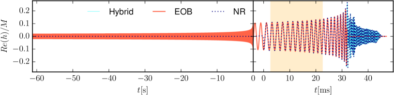
Figure 1: A hybrid waveform used in this study, with $M_{A}=M_{B}=1.35\,M_{\odot}$ and employing the SLy EOS. The hybrid (thin, cyan line) consists of a tidal EOB part (red) and an NR part (dotted blue). The alignment interval is marked by the yellow shaded region in the right panel. The time $t=0$ denotes the start of the NR simulation.

III.1 EOB waveform

We use the TEOBResum waveform model in the frequency regime from $30$ Hz to $\sim$500 Hz. TEOBResum is determined by seven input parameters: the binary mass-ratio $q$ and the $\l=2,3,4$ tidal polarizability parameters $\kappa^{A,B}_{\ell}$. The latter are related to the $\Lambda^{A,B}_{\ell}$ tidal deformability parameters by

$$\kappa^{A}_{\ell} =q^{-1}\ X_{A}^{2\ell+1}\ (2\ell-1)!!\ \Lambda^{A}_{\ell},$$ (4)

$$\kappa^{B}_{\ell} =q\ X_{B}^{2\ell+1}\ (2\ell-1)!!\ \Lambda^{B}_{\ell}\ ,$$ (5)

with $X_{A,B}=M_{A,B}/(M_{A}+M_{B})$. For our equal-mass ($M_{A}=M_{B}=1.35$) SLy and MS1b fiducial BNSs, one has $\kappa^{A}_{2}=\kappa_{2}^{B}=36.7749$ and $\kappa^{A}_{2}=\kappa_{2}^{B}=144.0378$ respectively.

Using the publicly available TEOBResum code, we generate waveforms starting at a frequency of $30$ Hz, which corresponds to $\sim$60 seconds before the time of merger. We restrict our analysis to the dominant $(2,2)$ mode throughout the paper.

III.2 Numerical-relativity data

The numerical simulations were performed with the BAM code Brügmann et al. (2008); Thierfelder et al. (2011), which solves the Einstein equations using the Z4c decomposition Bernuzzi and Hilditch (2010); Hilditch et al. (2013), and have been previously published in Ref. Bernuzzi et al. (2015a). The NR data are publicly available at http://www.computational-relativity.org/, cf. Dietrich et al. (2018b).

The two binary configurations used in this work describe equal-mass BNS systems with a total mass of $2.70\,M_{\odot}$, i.e., a chirp mass $\mathcal{M}=(M_{A}M_{B})^{3/5}/(M_{A}+M_{B})^{1/5}=1.1752\,M_{\odot}$. The two waveforms differ in their choice of the EOS modeling the supranuclear matter inside the NS. The NR waveforms start at an initial dimensionless frequency $(M_{A}+M_{B})\omega_{22}=0.038$, which corresponds to $455$ Hz. They cover $\sim$10 orbits prior to merger, the merger itself, and post-merger. The merger frequencies $f_{\rm merger}$ are $2010$ Hz and $1405$ Hz for waveforms with the SLy and the MS1b EOS, respectively, and the frequency content of the post-merger signal reaches up to $\sim 4000$ Hz. At the moment of merger, the phase uncertainty as estimated in Bernuzzi et al. (2015a) is $\Delta\phi=\pm 0.40\,$rad for the SLy and $\Delta\phi=\pm 3.01\,$rad for the MS1b setup. The larger phase uncertainty of the MS1b setup gets partially compensated for by the fact that this setup has also significantly larger tidal effects due to the stiffer EOS. For a more detailed discussion about uncertainties in NR simulations, we refer to Ref. Bernuzzi and Dietrich (2016).

III.3 Hybrid waveform

To hybridize the tidal EOB and NR waveforms modeling the same physical BNS system, we first align the two waveforms. This is done by minimizing

$$\mathcal{I}(\delta t,\delta\phi)=\int_{t_{i}}^{t_{f}}dt|\phi_{\rm NR}(t)-\phi_{\rm EOB}(t+\delta t)+\delta\phi|^{2},$$ (6)

with $\delta\phi$ and $\delta t$ being relative phase and time shifts. $\phi_{\rm NR}$ and $\phi_{\rm EOB}$ denote the phases of the NR and tidal EOB waveform, respectively. The alignment is done in a time window $[t_{i},t_{f}]$ that corresponds to the dimensionless frequency window $[0.04,0.06]$. Previous comparisons have shown that in this interval the agreement between the NR and EOB waveforms is excellent Bernuzzi et al. (2015a); Hotokezaka et al. (2015); Dietrich and Hinderer (2017). Additionally, our particular choice for this window allows us to average out the phase oscillations linked to the residual eccentricity $(∼10^{-2})$ of the NR simulations.

Once the waveforms are aligned, they are stitched together by the smooth transition

$$h_{\rm Hyb}(t)$$

$$=\left\{\small\begin{array}[]{ll}h_{\rm EOB}(t^{\prime})e^{i\phi}&:t\leq t_{i}\\ h_{\rm NR}(t)H(t)+h_{\rm EOB}(t^{\prime})e^{i\phi}[1-H(t)]&:t_{i}\leq t\leq t_{f}\\ h_{\rm NR}(t)&:t\geq t_{f}\end{array}\right.$$ (10)

where $t^{\prime}=t+\delta t$, and $H(t)$ is the Hann window function

$$H(t):=\frac{1}{2}\bigg{[}1-\cos\bigg{(}\pi\frac{t-t_{i}}{t_{f}-t_{i}}\bigg{)}\bigg{]}\,.$$ (11)

To estimate the uncertainty of the hybrid waveform, we present in Fig. 2 the same configuration, but evolved with different resolutions for the NR simulation and different time resolutions $\rm dt$ for the ordinary-differential-equation (ODE) integrator used in the TEOBResum model. We denote the high resolution NR simulations in which $\sim 128$ grid points cover the NS and in which we use $\rm dt=0.50$ for the EOB as $\rm Hyb_{1}$ (blue line in the top panel). $\rm Hyb_{2}$ is the hybrid employing a lower resolution NR dataset with $\sim 96$ grid points covering the NS, but the same resolution for the EOB ODE integrator. $\rm Hyb_{3}$ is the hybrid with NR resolution of 128 grid points and $\rm dt=0.25$ for the EOB ODE integrator resolution. To check the accuracy of the hybrid, we compute the dephasing between these three cases and an error is shown in the bottom panel of Fig. 2. We define the error as

$${\rm err}=\sqrt[]{(\phi_{{\rm{Hyb_{1}}}}-\phi_{{\rm{Hyb_{2}}}})^{2}+(\phi_{{\rm{Hyb_{1}}}}-\phi_{{\rm{Hyb_{3}}}})^{2}}\,.$$ (12)

Here, $\phi_{\rm{Hyb}_{1}}$, $\phi_{\rm{Hyb}_{2}}$ and $\phi_{\rm{Hyb}_{3}}$ are the phases of hybrids $\rm Hyb_{1}$, $\rm Hyb_{2}$, and $\rm Hyb_{3}$, respectively. For the error computation, we aligned all three hybrids within the frequency interval [32, 34]Hz and then calculate the phase differences. We find that the difference between $\rm Hyb_{1}$ and $\rm Hyb_{2}$ is below $\sim 0.1$ radian and at merger well within the NR uncertainty (olive shaded region). The effect of the ODE integration within the EOB model is even smaller. However, this study does not include the systematic effects of the underlying EOB model, see Ref. Nagar et al. (2018) for further details.

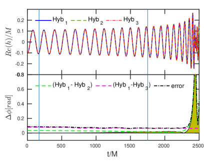
Figure 2: (Top panel) The three flavors of the hybrid discussed in Sec. III.3, each constructed with a different NR resolution and EOB integrator settings. Red and blue dashed curves represent the same NR resolution but a different EOB integrator setting. The green dashed curve has a lower NR resolution but same EOB integrator setting as for the red curve. The hybrid in Fig. 1 corresponds to the blue curve here. (Bottom panel) Phase difference between the hybrid of Fig. 1 and its two other realizations. The green dashed curve represents the absolute dephasing with the hybrid with low NR resolution, while the pink curve shows the absolute dephasing with the hybrid using a different EOB integrator setting. The black curve represents the absolute error defined in Eq. (12). The vertical lines mark the boundaries of the alignment window. The olive shaded region is the dephasing between two NR resolutions used.

IV Bayesian inference

In this section, we provide a brief overview of the Bayesian inference setup we use to determine the physical properties of the injected signal. The time series of detector data, $d(t)$, can be modeled as the sum of the true GW signal and detector noise, denoted by $h(t)$ and $n(t)$, respectively:

$$d(t)=h(t)+n(t).$$ (13)

Under this assumption, we can use Bayes’ theorem to determine the posterior probability density $p(\boldsymbol{\theta}|d(t))$ of the parameters $\boldsymbol{\theta}$, given the data $d(t)$ as

$$p(\boldsymbol{\theta}|d(t))\propto\mathcal{L}(d(t)|\boldsymbol{\theta})p(\boldsymbol{\theta})\,,$$ (14)

where $\mathcal{L}(d(t)|\boldsymbol{\theta})$ is the likelihood, or the probability of observing the data $d(t)$ given the signal model described by $\boldsymbol{\theta}$, and $p(\boldsymbol{\theta})$ denotes the prior probability density of observing such a source. For Gaussian noise, the likelihood for a single detector is given by Finn (1992)

$$\mathcal{L}(d(t)|\boldsymbol{\theta})\propto\exp\left[\ -2\int_{0}^{\infty}\frac{|\tilde{d}(f)-\tilde{h}(f,\boldsymbol{\theta})|^{2}}{S_{\rm det}(f)}df\right]\ ,$$ (15)

where tildes denote Fourier transforms of time series introduced so far and $S_{\rm det}(f)$ is the one sided PSD of the detector. Under the assumption that noise in different detectors is not correlated, this expression is readily generalized to the case of a coherent network of detectors by taking the product of the likelihoods in each detector Finn (1996).

Credible intervals for a specific subset of source parameters in the set $\boldsymbol{\theta}$ may be obtained by marginalising the full posterior over all but those parameters. Obtaining credible intervals therefore requires sampling the multidimensional space of source parameters. We do this with lalinference_mcmc, a Markov-Chain Monte Carlo sampler algorithm van der Sluys et al. (2008) included in the LALInference package Veitch et al. (2015) as part of the LSC Algorithm Library (LAL) Allen et al. (2010). In addition to the chirp mass, $\mathcal{M}$, the binary mass ratio, $q=M_{B}/M_{A}(\leq 1)$, the dimensionless spin magnitudes of the two NSs, $\chi_{A,B}$, the tidal deformability parameters, $\tilde{\Lambda}$ and $\delta\tilde{\Lambda}$ [Eqs. (2)-(3)], our parameter space also includes the luminosity distance, an arbitrary reference phase and time for the GW signal, the inclination angle of the binary with respect to the line-of-sight of the detectors, the polarization angle, and the right ascension and declination of the source, i.e., its sky location.

A key ingredient of Bayesian analyses is one’s choice of the prior probability density $p(\boldsymbol{\theta})$ (along with the hypothesis used to perform inference on the data, which in our specific case is the choice of the waveform model). We use a uniform prior distribution in the interval $[1M_{\odot},3M_{\odot}]$ for the component masses, and a uniform prior between $-1$ and $1$ for both dimensionless aligned spins. We also pick a uniform prior distribution for the individual tidal deformabilities $\Lambda_{2}^{A,B}$ between $0$ and $5000$ for all waveform models except TEOBResum_ROM, in which case they are bound between $50$ and $5000$. With regards to tidal deformability, our setup makes the simplifying assumption of ignoring correlations between $\Lambda_{2}^{A}$, $\Lambda_{2}^{B}$, and the mass parameters, which are known to exist Flanagan and Hinderer (2008); Hinderer et al. (2010); Favata (2014). For all other parameters we follow the setup of standard GW analyses, e.g., Abbott et al. (2018b).

V Results

EOS	$\tilde{\Lambda}$	$\mathcal{M}$ $[M_{\odot}]$	$\chi_{\rm eff}$	PSD	$f_{\rm high}$	SNR
SLy	392	1.1752	0.0	O1	2048 Hz	25
					2048 Hz	100
				ZDHP	2048 Hz	100
					8192 Hz	100
MS1b	1536	1.1752	0.0	O1	2048 Hz	25
					2048 Hz	100
				ZDHP	2048 Hz	100
					8192 Hz	100

Table 1: The eight injections used in this study. We consider two equal-mass, non-spinning BNS hybrid waveforms (see Sec. III) with the same chirp mass, but different EOS, and hence different tidal polarizability $\tilde{\Lambda}$. The SNR of each injection is specified in the seventh column. When assessing the impact of tidal effects on the analysis of a GW inspiral signal, we use the first observing run’s noise PSD. In such cases, the waveform models employed to recover the signal are IMRPhenomD_NRTidal, SEOBNRv4_ROM_NRTidal, TaylorF2_Tides, IMRPhenomD, TaylorF2, and TEOBResum_ROM. When assessing the impact of post-merger dynamics on GW inference, instead, we use the projected noise curve for the Advanced LIGO detectors in the ZDHP configuration, and IMRPhenomD_NRTidal and TaylorF2_Tides waveform models for the signal recovery. Given that the high-frequency content of the post-merger portion of the signal reaches $\sim 4$ kHz, we produce injections with sampling rates of $16384$ Hz and $4096$ Hz, and correspondingly use a high-frequency cutoff in our Bayesian analysis of $f_{\rm high}=8192$ Hz and $f_{\rm high}=2048$ Hz. The merger frequencies are $2010$ Hz and $1405$ Hz for waveforms with SLy and MS1b EOS, respectively.

We consider a two-detector network that consists of the LIGO interferometers situated in Hanford and Livingston, US. We inject the equal-mass SLy and MS1b hybrid GW signals discussed in Sec. III Schmidt et al. (2017). For each hybrid signal, we consider $4$ different injection setups, for a total of $8$ scenarios, as summarized in Table 1. To study the impact of neglecting/including tidal effects in the analysis of a BNS GW inspiral signal, we assume a noise PSD from the first observing run of the LIGO detectors and perform two injections per hybrid, with SNRs $25$ and $100$ [rows 1, 2, 5, and 6 in Table 1]. The former value allows us to address a scenario in which the source is detected with a moderately high SNR, namely $\sim 3$ times the detection threshold. An SNR of $100$ is chosen, instead, to assess the impact that tidal effects have on the recovery of BNS source properties for an extreme scenario. The same, high value of SNR is used when assessing the impact of post-merger dynamics on GW inference. For this scope, we assume the projected noise curve for the Advanced LIGO detectors in the ZDHP Shoemaker and Collaboration (2010). Because the high-frequency content of the post-merger portion of the GW reaches $\sim 4000$ Hz, we produce injections with two different sampling rates: $16384$ Hz and $4096$ Hz, which correspond to a high-frequency cutoff in our Bayesian analysis of $f_{\rm high}=8192$ Hz and $f_{\rm high}=2048$ Hz, respectively (rows 3, 4, 7, and 8 in Table 1). In all cases, no actual noise is added to the data. This allows us to obtain posteriors that do not depend upon a specific noise realization, therefore isolating systematic errors. All injections start at a frequency of $30$ Hz, while our Bayesian analysis uses a low cutoff frequency $f_{\rm low}=32$ Hz to generate template waveforms. As discussed in Sec. II, we use a number of different waveform approximants for estimating parameters; this allows us to qualitatively assess systematic errors present in such waveform models. As opposed the full inspiral-merger-post–merger BNS signals we inject, the waveform models used for estimating parameters are limited to the inspiral regime.

The insights we gained by comparing the results of parameter estimation using different waveform models are summarized in the following subsections.

V.1 Effects of tidal terms

We first assess under what conditions neglecting tidal effects incurs a bias in the recovered masses and spins, and then investigate configurations where uncertainties in the modeling of tidal effects can incur a bias in both the masses and spins, and the measurement of the tidal deformability.

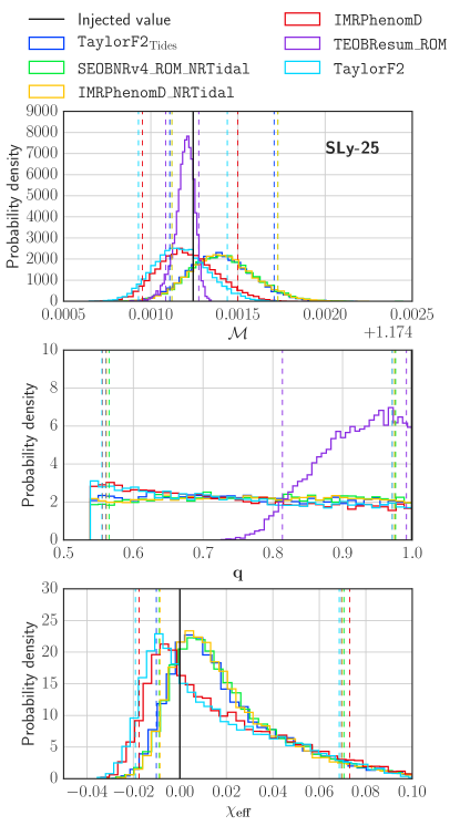
Figure 3: The chirp mass $\mathcal{M}$ (top panel), mass ratio $q$ (middle panel), and effective spin $\chi_{eff}$ (bottom panel) posterior distributions for the BNS injection with SLy EOS at SNR 25. The vertical dashed lines mark the $90$% credible intervals, while the solid black line indicates the injected value.

The waveform phase evolution is dominated by the chirp mass Peters and Mathews (1963), followed by the mass-ratio $q$, and then spin effects. The spins are characterized in parameter measurements by a weighted sum of the two spins, $\chi_{\rm eff}$ Ajith et al. (2011),

$$\chi_{\rm eff}=\frac{M_{A}\chi_{A}+M_{B}\chi_{B}}{M_{A}+M_{B}},$$ (16)

which is related to the leading-order PN spin contribution to the waveform phase Kidder et al. (1993). There is a partial signal degeneracy between the mass-ratio and the spin Cutler and Flanagan (1994); Poisson and Will (1995); Baird et al. (2013); Hannam et al. (2013); Ohme et al. (2013), in that increased spin can be compensated by a lower mass ratio; the degeneracy is not exact because mass-ratio and spin effects enter at different PN order. Tidal effects enter at yet higher (5PN) order, but can also be partially mimicked by a change in mass ratio and spin; thus, neglecting tidal effects could lead to a bias in $\chi_{\rm eff}$ and in the mass ratio. We will investigate the extent of these biases in the following, by considering the recovery of the chirp mass, $\mathcal{M}$, the mass-ratio $q$, and $\chi_{\rm eff}$.

We first consider the SLy configuration observed with an SNR of 25; note that the GW170817 observation was at a comparable SNR of 32.4, and the SLy configuration has a tidal deformability of $\tilde{\Lambda}=392$, also consistent with the measurements of GW170817 Abbott et al. (2018b). Figure 3 shows the chirp mass $\mathcal{M}$, mass-ratio $q$ and effective spin $\chi_{\rm eff}$. We see that the injected value of the chirp mass is inside the 90% credible interval for all approximants used to recover the injected signal. The chirp-mass (and mass-ratio) posterior distribution yielded by the TEOBResum_ROM approximant is significantly different from the other ones. This is due to the fact that this waveform model is non-spinning; the parameter estimation algorithm therefore explores a parameter space that differs from the one it handles in the case of all other approximants. With the exception of TEOBResum_ROM, the peak of the chirp-mass distribution is slightly higher than the injected chirp-mass value for approximants that include tidal terms, but it is shifted to lower values for the approximants that neglect tidal terms. The degeneracy between mass-ratio and spin leads to a relatively flat distribution in $q$ for all approximants; although there is a hint that the posterior is starting to rail against the lower prior limit of $q$ in the parameter estimation run, the effect is small. The effect of this degeneracy is most clearly illustrated by the results from the TEOBResum_ROM approximant, which, once more, is a non-spinning approximant, and without this degree of freedom the mass ratio is recovered with far greater accuracy. In measurements of the spin, the peak of the distribution is again slightly shifted away from the injected value, towards lower values for non-tidal approximants and towards higher values for tidal approximants. Once again, the injected values lie within the 90% credible interval.

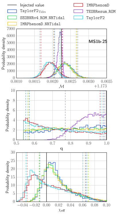
Figure 4: Same as Fig. 3 but assuming the MS1b EOS to produce the injected BNS signal.

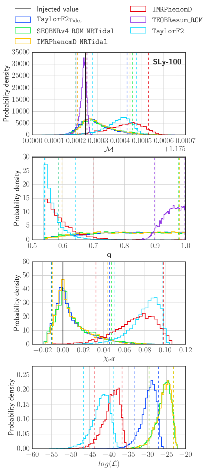
Figure 5: Same as Fig. 3, but with an injected SNR of 100. We also show the distribution of the logarithm of the likelihood in the bottom panel.

We conclude that for soft EOSs at this SNR, neglecting tidal terms does not lead to a significant bias in measurements of masses and spins.

This picture changes when we consider a stiffer EOS. Figure 4 shows the same quantities, but for the MS1b configuration ($\tilde{\Lambda}=1536$) injected at SNR 25. Although the 90% credible intervals for the mass ratio and spin agree with the injected values, the bias in the measurement of the chirp mass obtained with non-tidal approximants is more significant: the injected value is outside the 90% credible interval for TaylorF2, and it is very close to the edge of the 90% credible interval for IMRPhenomD. Further, the peak of the mass-ratio distribution is railing more significantly against the lower prior limit in the case of the non-tidal approximants, and, similarly, we observe an increase in the shift of the peak of the spin distribution for the same waveform models. Collectively, these results indicate that for stiff EOSs neglecting tidal terms does lead to a bias in the measurement of the masses and spins.

Assuming future observations will be similar to GW170817 ($\tilde{\Lambda}<720$ Abbott et al. (2018b)) and that SNRs higher than 25 will be rare, our results suggest that neglecting tidal effects will not significantly bias measurements of masses and spins for typical observations. However, careful analyses will be required once individual events are combined to extract information about the BNS population as a whole.

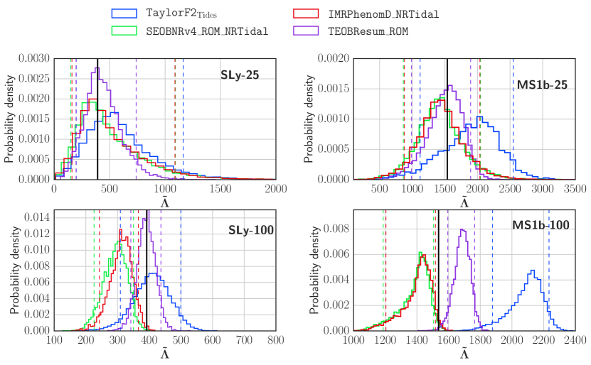
Figure 6: Measurements of the tidal deformability parameter. The two panels on the left show results for the SLy signal injected at SNR 25 (top) and 100 (bottom). The two panels on the right show results for the MS1b signal injected at SNR 25 (top) and 100 (bottom).

We also investigate how these results change for a much higher SNR. Figure 5 shows measurements of the chirp mass, mass ratio and spin for the SLy configuration, now injected at an SNR of 100. We see that the chirp mass is now biased away from the correct value for the two approximants that do not include tidal terms. When estimating the parameters, we enforced a limit that $m_{1,2}\in[1,3]M_{\odot}$, which implies $\mathcal{M}_{c}\in[0.8706,2.6117]M_{\odot}$. The parameter estimation code adjusts the masses and spins to find the best match with the data, and for those approximants that do not include tidal terms, the search rails against the limits on the masses, as well as on the physical limit $\chi\leq 1$ for the spins. This is most clear in the plot of the posterior distribution for $q$. The Figure also includes a plot of the logarithm of the likelihood; we see that the TaylorF2 and IMRPhenomD approximants cannot be made to match the data as accurately as the tidal approximants, and so their likelihoods are lower. (More generous limits on the masses in the parameter recovery may lead to a higher likelihood for these approximants, but we do not expect it to be as high as for the approximants that include tidal terms, since biases in the masses and spins can only partially mimic the missing tidal effects.) We also see that the TaylorF2_Tides approximant, although it contains tidal terms, is not as accurate as the NRTidal approximants, for which the tidal terms have been tuned to NR waveforms.

We now move on to measurements of the tidal deformability, $\tilde{\Lambda}$, for which we can compare the accuracy of different tidal approximants. In Fig. 6, the left two panels show the results for SLy injections (at SNRs 25 and 100), and the two right panels show the results for MS1b. The results shown here are entirely consistent with the systematics tests performed for the LIGO-Virgo Collaboration analysis of the properties of GW170817 Abbott et al. (2018b). In particular, all tidal approximants agree within their 90% credible intervals at SNRs measured to date, for both soft and stiff EOSs, and for all configurations the TaylorF2_Tides approximant can be used to place an upper bound on $\tilde{\Lambda}$, as in Refs. Abbott et al. (2017a); Abbott et al. (2018b).

It is interesting to note, however, the at an SNR of 100, the measurement using the NRTidal approximants is biased away from the injected value of the hybrid, which was constructed from the TEOBResum approximant. This is an indication that we do not have sufficient control over systematics for high-SNR setups. A possible explanation for this behavior is that tidal effects in the NRTidal model are larger than in the TEOBResum model used to produce the injected signals, as already highlighted in Fig. 10 of Ref. Dietrich et al. (2018a). Another possible explanation is that this is due to differences between the NRTidal and TEOBResum approximants in the BH limit. The agreement of TaylorF2_Tides in the bottom-left panel of Fig. 6 is accidental. (We believe that this is due to a compensation of two effects: TaylorF2_Tides models underestimating tidal effects and therefore overestimating $\tilde{\Lambda}$, and systematics errors in the point-particle description Messina et al. (2018).) We note also that at SNR 100, the TEOBResum approximant provides a biased measurement for MS1b. This may be surprising at first, since TEOBResum was used in the construction of the MS1b hybrid, but the approximant is used only up to the hybridisation frequency, from which point onwards the NR waveform is used. There is an SNR of $\sim 16$ from the hybridization frequency up to the merger. As already stated, there are also systematic differences between TEOBResum and TEOBResum_ROM Lackey et al. (2017). We found a phase difference between our hybrid and the waveform generated using TEOBResum_ROM of about $\sim 4$ rad at merger for the MS1b case and $\sim 0.8$ rad for the SLy case. We suggest this to be the reason for the offset between the injected value and the TEOBResum_ROM result at ${\rm\acs{SNR}}=100$, cf. Fig. 6.

V.2 Effect of postmerger

We now investigate whether the lack of the post-merger part of the signal in the models, which we use for Bayesian inference, could lead to biases in parameter measurements. Previous studies of post-merger GW signals Clark et al. (2015); Bose et al. (2018); Chatziioannou et al. (2017) suggest that this portion of the signal would be detectable, and its properties measurable, only if the SNR of the post-merger regime alone were above $\sim 5$. Recently, Chatziioannou et al. (2017) found that for soft EOSs an SNR of $3$–$4$ might be sufficient for a detection of the post-merger GW using the BayesWave algorithm Cornish and Littenberg (2015). In this article, we assume a threshold SNR of $5$ to produce more conservative estimates. Figure 7 shows the accumulated SNR of the post-merger regime for our SLy and MS1b configurations at a total signal SNR of 100. In order to achieve a post-merger SNR of 5, we would need a total signal SNRs of approximately 185 and 250, for the MS1b and SLy EOSs, respectively. These would correspond to source distances of 17 Mpc and 13 Mpc. If we assume an SNR signal detection threshold of 10 and a uniform volume distribution of sources throughout the universe, then only about 1 in every 6000 observations will have an SNR greater than 185. This suggests that it is unlikely for Advanced LIGO and Virgo detectors to be able to measure post-merger signals, and that it is therefore extremely unlikely that the post-merger part that is absent from our signal models will bias the parameter recovery from the inspiral waveform. Nonetheless, our hybrid waveforms provide the opportunity to conclusively test this expectation, and that is what we do in this section.

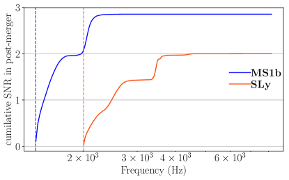
Figure 7: SNR accumulated during the post-merger regime as a function of frequency. The vertical lines indicate the merger frequency, where the computation of the SNR starts. Blue and red curves correspond to the hybrid being injected. The ZDHP projected noise curve for the Advanced LIGO detectors is used.

To quantify the impact of the post-merger portion of the signal, we injected full, hybrid waveforms at ${\rm\acs{SNR}}=100$ and compared results obtained using upper cutoff frequencies $f_{\rm high}=2048$ Hz and $f_{\rm high}=8192$ Hz. The merger frequencies $f_{\rm merger}$ are $2010$ Hz and $1405$ Hz for waveforms with the SLy and the MS1b EOS, respectively, and the frequency content of the post-merger signal reaches up to $\sim 4000$ Hz, with peak frequencies at $f_{1}$ $\sim 2600$ Hz and $f_{2}$ $\sim 3400$ Hz for SLy, and $f_{1}$ $\sim 1600$ Hz and $f_{2}$ $\sim 2100$ Hz for MS1b. We find that the results of parameter estimation for the two different cutoff frequencies are remarkably in agreement with each other, suggesting that the lack of post-merger content in the models used for parameter estimation has no impact on the recovery for this configuration. Figure 8 shows that the recovered SNR is insensitive to the upper cutoff frequency, i.e., to the presence/absence of post-merger content in the injected signal, and to the waveform model used in the recovery, since results for IMRPhenomD_NRTidal and TaylorF2_Tides are quite close. Further, in all four cases the full injected SNR is recovered. The $\sim 2$% drop from the nominal injected SNR of 100 to ${\rm\acs{SNR}}=98$ is due to the fact that while the injected signal starts at $30$ Hz, the filtering against the template waveform has a minimum frequency of $32$ Hz.

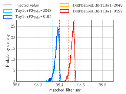
Figure 8: The matched filter SNR recovered by TaylorF2_Tides and IMRPhenomD_NRTidal for the EOS-MS1b hybrid injected at SNR=100, using two different sampling rates for the templates, namely, $4096$ Hz and $16384$ Hz. Vertical dashed lines indicate $90\%$ credible intervals, while the black solid line marks the injected value.

Figure 9 shows the posterior distribution for $\tilde{\Lambda}$ for both choices of upper cutoff frequency, for the SLy (upper panel) and MS1b (bottom panel) configuration injected at $\rm\acs{SNR}=100$, using the IMRPhenomD_NRTidal and TaylorF2_Tides waveform models. The upper cutoff frequency, or equivalently the inclusion or absence of the post-merger regime in the injected signal, has negligible effect on the results. As was the case for the ${\rm{\acs{SNR}}}=100$ injections performed with the second observing run noise PSD, the NRTidal models underestimate $\tilde{\Lambda}$ for all injections. For an explanation, we refer the reader to V.1.

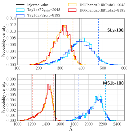
Figure 9: Tidal deformability posterior distributions found when injecting the SLy EOS (top panel) and the MS1b EOS (bottom panel) BNS hybrids at SNR $100$. The recovery is performed the IMRPhenomD_NRTidal and TaylorF2_Tides approximants with sampling rates $16384$ Hz and $4096$ Hz. Vertical dashed lines indicate $90\%$ credible intervals, while the black solid lines mark the injected values.

These results are consistent with our expectation that the post-merger will have negligible impact on our parameter recovery with the current generation of interferometric GW detectors.

VI Conclusion

In this work, we considered two possible sources of systematic uncertainties in the Bayesian parameter estimation of the GW signal emitted by a coalescing BNS. We focused on two questions: (i) What is the impact of neglecting tidal effects in the analysis of the inspiral GW signal? (ii) Does the use of inspiral-only waveforms lead to a significant loss of information, or possibly to biases in the estimation of the source properties? To answer these questions, we produced complete BNS GW signals by combining state-of-the-art EOB waveforms for the inspiral, and NR simulations of the late inspiral and merger (see Sec. III), we injected such signals into fiducial data streams of the LIGO detectors (see Table 1), and, finally, we used the parameter-estimation algorithm LALInference Veitch et al. (2015); Allen et al. (2010)) to extract the source properties from the data streams containing the injected signals. We addressed the first question by filtering the data with a variety of theoretical waveforms, with and without tidal effects, whereas to address the second question we quantified the importance of the post-merger part of the signal by measuring its SNR.

We showed that neglecting tidal effects in the inspiral waveforms used to infer the source properties does not bias measurements of masses and spin for a canonical observation at SNR=25, as long as the NS EOS is fairly soft ($\tilde{\Lambda}\lesssim 400$). In the high SNR regime and/or for stiff EOSs ($\tilde{\Lambda}\sim 1500$), however, there will be a significant bias in the measurements of masses and spins when inspiral waveform models that do not include tidal effects are used (Figs. 4 and 5).

We also found that the recovery of chirp mass $\mathcal{M}$, mass-ratio $q$, effective spin $\chi_{\rm eff}$, and tidal deformability $\tilde{\Lambda}$ is consistent among all tidal models that include tidal effects for an injected SNR of $25$ for both soft and stiff EOSs. In this context, TaylorF2_Tides overestimates the recovered value of $\tilde{\Lambda}$, as stated in the analysis of GW170817 Abbott et al. (2018b). This is due to TaylorF2_Tides favouring larger values of $\tilde{\Lambda}$ in order to compensate for the smaller tidal effects it includes in the phasing of the late inspiral regime when compared to NRTidal models Dietrich et al. (2018a). At high SNR, the impact of systematics present in the various waveform models increases. In particular, the bottom panels of Fig. 6 show that NRTidal models yield a conservative lower estimate of $\tilde{\Lambda}$. It is not clear whether the differences between the NRTidal and TEOBResum approximants are dominated by differences in the BH ($\tilde{\Lambda}\rightarrow 0$) limit, or in the description of tidal effects, and this requires further study.

Considering the possibility for upcoming detections with large SNRs due to the increasing sensitivity of advanced GW detectors our study showed the importance to further improve BNS waveform models in coming years.

To investigate the impact of neglecting the post-merger portion of the signal in waveform models used for parameter estimation of BNS signals, we calculated the SNR of the post-merger regime. As suggested in Refs. Clark et al. (2015); Bose et al. (2018); Chatziioannou et al. (2017) this part of the signal would be detectable, and its properties measurable, only if its SNR were above $\sim 5$. As shown in Fig. 7, achieving SNR $\sim 5$ in the post-merger regime requires a total SNR of about $\sim 200$. The odds of having an event with SNR $\sim 200$ are 1 in every 6000 observations. This makes it unlikely for second generation detectors to measure the post-merger part of BNS GW signals, and thus the absence of the post-merger regime in waveform models currently used in Bayesian inference is not worrisome for Advanced LIGO and Virgo.