Gravitational-wave signal from binary neutron stars: a systematic analysis of the spectral properties

Abstract

A number of works have shown that important information on the equation of state of matter at nuclear density can be extracted from the gravitational waves emitted by merging neutron-star binaries. We present a comprehensive analysis of the gravitational-wave signal emitted during the inspiral, merger and post-merger of 56 neutron-star binaries. This sample of binaries, arguably the largest studied to date with realistic equations of state, spans across six different nuclear-physics equations of state and ten masses, allowing us to sharpen a number of results recently obtained on the spectral properties of the gravitational-wave signal. Overall we find that: (i) for binaries with masses differing no more than $20\%$, the frequency at gravitational-wave amplitude’s maximum is related quasi-universally with the tidal deformability of the two stars; (ii) the spectral properties vary during the post-merger phase, with a transient phase lasting a few millisecond after the merger and followed by a quasi-stationary phase; (iii) when distinguishing the spectral peaks between these two phases, a number of ambiguities in the identification of the peaks disappear, leaving a simple and robust picture; (iv) using properly identified frequencies, quasi-universal relations are found between the spectral features and the properties of the neutron stars; (v) for the most salient peaks analytic fitting functions can be obtained in terms of the stellar tidal deformability or compactness. Altogether, these results support the idea that the equation of state of nuclear matter can be constrained tightly when a signal in gravitational waves from binary neutron stars is detected.

I Introduction

The recent measurement from the advanced interferometric LIGO detectors (Harry et al., 2010) of the first direct gravitational-wave (GW) signal from what has been interpreted as the inspiral, merger and ringdown of a binary system of black holes Abbott et al. (2016) marks, in many respects, the beginning of GW astronomy. As additional advanced detectors such as Virgo (Accadia et al., 2011), and KAGRA (Aso et al., 2013) are going to become operational in the next few years, we are likely to soon witness also signals from the inspiral and post-merger of neutron-star binaries or neutron-star–black-hole binaries. Such systems are not only excellent sources of GWs, but also the most attractive scenario to explain the phenomenology associated with short gamma-ray bursts (SGRBs). Starting from the first suggestions that merging neutron stars could be behind these phenomena Narayan et al. (1992); Eichler et al. (1989) and supported by the circumstantial evidence coming from numerous astronomical observations (see Berger (2014) for a recent review), numerical simulations have sharpened the contours of this scenario Shibata and Uryū (2000); Baiotti et al. (2008); Anderson et al. (2008a); Liu et al. (2008); Bernuzzi et al. (2012a). What we now know rather reliably is that the merger of a binary neutron-star (BNS) system inevitably leads to the formation of a massive metastable object, which can either collapse promptly to a black hole or survive up to thousands of seconds Ravi and Lasky (2014), emitting gravitational and electromagnetic radiation Zhang and Mészáros (2001); Metzger et al. (2011); Rezzolla and Kumar (2015); Ciolfi and Siegel (2015). Furthermore, if the neutron stars have large magnetic fields and extended magnetospheres, the inspiral can be accompanied by a precursor electromagnetic signal Palenzuela et al. (2013), while the merger can lead to instabilities Siegel et al. (2013); Kiuchi et al. (2015) and to the formation of magnetically confined jet structures once a torus is formed around the black hole Rezzolla et al. (2011); Paschalidis et al. (2015). Hence, the prospects of a multimessenger gravitational and electromagnetic signal are particularly good in the case of merger of binary neutron stars.

In addition to a strong electromagnetic signal, the merger of a neutron-star binary also promises a GW signal that will contain important signatures of the equation of state (EOS) of matter at nuclear densities. These signatures are contained both in the inspiral and in the post-merger signals. The former is reasonably well understood analytically Flanagan and Hinderer (2008); Baiotti et al. (2010); Bernuzzi et al. (2012b, 2015a); Hinderer et al. (2016) and can be tracked accurately with advanced high-order numerical codes Radice et al. (2014a, b, 2015) and over many orbits now Hotokezaka et al. (2016). More importantly, the instantaneous GW frequency at amplitude maximum $f_{\rm max}$ has been shown to correlate closely with the tidal deformability of the two stars Read et al. (2013); Bernuzzi et al. (2014a); Takami et al. (2015). The latter part of the signal has already been studied in the past Shibata (2005); Oechslin and Janka (2007); Baiotti et al. (2008), but it has become the focus of attention particularly over the last few years Bauswein and Janka (2012); Stergioulas et al. (2011); Bauswein et al. (2012); Hotokezaka et al. (2013); Bauswein et al. (2014); Takami et al. (2014, 2015); Bernuzzi et al. (2015b); Palenzuela et al. (2015); Bauswein and Stergioulas (2015); Dietrich et al. (2015); Foucart et al. (2016); Lehner et al. (2016). This large bulk of work has reached some generally agreed-upon conclusions, but also has raised points that are a matter of debate that we hope to clarify here.

Let us therefore start by summarising the aspects of the post-merger GW signal that seem to be robust and confirmed by several groups employing a variety of numerical methods and mathematical approximations. Given a realistic BNS system, namely, with a total mass between $\sim 2.4$ and $\sim 2.8\,M_{\odot}$, and a mass difference between the two components that is $\sim 20\%$ or less, then the spectrum of the post-merger GW signal will present at least three strong peaks Bauswein and Janka (2012); Stergioulas et al. (2011); Bauswein et al. (2012); Hotokezaka et al. (2013); Bauswein et al. (2014); Takami et al. (2014, 2015). These peaks were dubbed $f_{1},f_{2}$ and $f_{3}$ in Refs. Takami et al. (2014, 2015) and were found to satisfy the following approximate relation: $f_{2}\simeq(f_{1}+f_{3})/2$. A simple mechanical toy model was also presented in Takami et al. (2015), that provided an intuitive explanation on the origin of these peaks and why they should be almost equally spaced. In addition to these three peaks, another peak can be identified in the power spectral density (PSD) of the GW signal, although not always. This is given by the coupling between the $\ell=2=m$ fundamental mode (which yields the $f_{2}$ peak) and a quasi-radial (fundamental) axisymmetric mode, i.e., with $\ell=2,m=0$; this mode was dubbed $f_{2\mbox{-}0}$ in Ref. Stergioulas et al. (2011). Finally, Ref. Bauswein and Stergioulas (2015) introduced the concept of the $f_{\rm spiral}$ peak frequency and associated it to a “rotating pattern of a deformation of spiral shape”. It is difficult to measure this motion in a numerical-relativity calculation without the possible contamination of spatial-gauge effects; however, as we will show in the following, $f_{\rm spiral}$ coincides with $f_{1}$ in the large majority of the cases so that, in the end, the strongest and most robust features of the post-merger signal are confined to four frequencies: $f_{1},f_{2},f_{3}$, and $f_{2\mbox{-}0}$, respectively.

In addition to selecting the most salient spectral features of the post-merger GW signal, the analyses of Refs. Bauswein and Janka (2012); Stergioulas et al. (2011); Bauswein et al. (2012); Hotokezaka et al. (2013); Bauswein et al. (2014); Takami et al. (2014, 2015); Bernuzzi et al. (2015b) have also tried to associate the values of these frequencies to the stellar properties of the two stars before the merger and hence to their EOS. This was initiated by Refs. Bauswein and Janka (2012); Bauswein et al. (2012), who showed that $f_{2}$ correlated with the radius of the maximum-mass nonrotating configuration; the correlation found was rather tight, but restricted to binaries having all the same total mass of $2.7\,M_{\odot}$ Bauswein and Janka (2012); later on, the correlation was explored also when considering a larger sample of masses Bauswein et al. (2012), and it was noted that the correlation was not as tight as previously expected. Indeed, Refs. Takami et al. (2014, 2015) discovered that the correlations of the $f_{2}$ peaks with the radius of the maximum-mass nonrotating configuration depend on the total mass of the system and hence are not “universal” in the sense of being only weakly dependent on the EOS (see also Refs. Bauswein et al. (2012); Hotokezaka et al. (2013)). At the same time, Refs. Takami et al. (2014, 2015) showed that the $f_{1}$ peak is correlated with the total compactness of the stars in a quasi-universal manner, and highlighted a number of other correlations (24 different ones were presented in Fig. 15 of Takami et al. (2015)); some of these correlations had been already presented in the literature, e.g., in Refs. Read et al. (2013); Bernuzzi et al. (2014a), while most of them were presented there for the first time. More specifically, correlations were found between $f_{\rm max},f_{1}$ and $f_{2}$ frequencies and the physical quantities of the binary system, e.g., the stellar compactness, the average density, or the dimensionless tidal deformability (some of these correlations will be further discussed below).

Some of the results reviewed above are robust, while other are less so. In particular, although the interpretation of the largest peak in the spectrum is normally attributed to the $\ell=2=m$ mode of the HMNS, the interpretation of the low-frequency peak (or peaks) is still subject to debate. More specifically, it is unclear whether such a peak (or peaks) correlates in a “universal” manner with the stellar properties, as shown in Takami et al. (2015) for the $f_{1}$ peak, or not, as shown in Bauswein and Stergioulas (2015) for the $f_{\rm spiral}$ peak.

The purpose of this paper is to try and clarify this debate and, more specifically, to show that for the cases considered here the $f_{\rm spiral}$ frequency either coincides with the $f_{1}$ frequency or falls in a part of the PSD of the signal where no significant power can be found, thus explaining why no universal behaviour was found in Ref. Bauswein and Stergioulas (2015). We reach this conclusion by extending the sample of binaries considered in Refs. Takami et al. (2014, 2015) to include the fully general-relativistic simulations of the very low-mass binaries with total mass $2\times 1.2\,M_{\odot}$ and that were suggested by Bauswein and Stergioulas (2015) to be missing in our sample. In addition, we also consider the largest masses that can be supported for a timescale after the merger sufficiently long to yield an accurate spectrum; depending on the EOS, these masses can be as large as $2\times 1.5\,M_{\odot}$. The large majority of binaries have equal masses, but we consider also four different instances of unequal-mass binaries with mass difference of about $20\%$.

This complete sample of binaries, which counts a total of 56 binaries and doubles the sample presented in Takami et al. (2015), is arguably the largest studied to date with nuclear-physics EOSs and in full general relativity (a sample of comparable size but not in full general relativity was already presented in Ref. Bauswein et al. (2012)). After a systematic analysis of the complete sample, it was possible to sharpen a number of arguments on the spectral properties of the GW signal and that can be summarised as follows:

• the GW frequency at amplitude maximum $f_{\rm max}$ is related to quasi-universally with the tidal deformability of the two stars; this correlation is strong for equal-mass binaries and holds as long as the binaries have masses that do not differ of more than $20\%$.

• the post-merger signal is characterised by a transient phase lasting a few millisecond after the merger, which is then followed by quasi-stationary phase.

• the spectral properties of the GW signal vary during the post-merger phase with a marked difference between the transient and the quasi-stationary phase.

• spectrograms are particularly useful when selecting spectral features in the transient phase because peaks that appear in the short transient, may be subdominant when analysed in terms of the full PSD.

• when distinguishing the spectral peaks between the transient and quasi-stationary phases, a number of ambiguities in the identification of the peaks disappear, leaving a rather simple and robust picture;

• the strongest and most robust features of the post-merger signal are confined to four frequencies: $f_{1},f_{2},f_{3}$, and $f_{2\mbox{-}0}$, where $f_{2}\simeq(f_{1}+f_{3})/2$ and $f_{2\mbox{-}0}$ is the result of a mode coupling.

• a number of “universal” relations can be found between the main spectral features and the physical properties of the neutron stars.

• for all of the correlations found, simple analytic expressions can be given either in terms of the dimensionless tidal deformability or of the stellar compactness.

When considered as a whole, these results support the idea that the equation of state of nuclear matter can be tightly constrained when a strong post-merger signal in GWs is measured.

The paper is organised as follows. Section II provides a very brief summary of the mathematical and numerical methods used to obtain our results in full general relativity, while Sect. III is dedicated to the illustration of our results. In particular, in Sects. III.1, III.2, and III.3 we concentrate on the waveform properties coming from transient signals, quasi-stationary signals and from the analysis of the full PSDs, respectively. The analysis of the correlations of the spectral signatures with the stellar properties is instead presented in Sect. III.4, while Sect. IV contains our conclusions and future prospects. Three different appendices offer details on the full set of binaries considered (Appendix A), on the analysis of some modes (Appendix B) or on a two-dimensional fit employed in our analysis (Appendix C).

II Mathematical and numerical Setup

The mathematical and numerical setup used for the simulations reported here is the same discussed in Takami et al. (2014, 2015) and presented in greater detail in other papers Baiotti et al. (2008, 2009, 2010). For completeness we review here only the basic aspects, referring the interested reader to the papers above for additional information. All of our simulations have been performed in full general relativity using a fourth-order finite-differencing code McLachlan Brown et al. (2009); Löffler et al. (2012), which solves a conformal traceless formulation of the Einstein equations Nakamura et al. (1987); Shibata and Nakamura (1995); Baumgarte and Shapiro (1999), with a “$1+\log$” slicing condition and a “Gamma-driver” shift condition (Alcubierre et al., 2003; Pollney et al., 2007). At the same time, the general-relativistic hydrodynamics equations are solved using the finite-volume code Whisky (Baiotti et al., 2005), which has been extensively tested in simulations involving the inspiral and merger of BNSs Baiotti et al. (2008, 2009); Rezzolla et al. (2010); Baiotti et al. (2010).

The hydrodynamics equations are solved employing the Harten-Lax-van Leer-Einfeldt (HLLE) Harten et al. (1983) approximate Riemann solver Harten et al. (1983), which is less accurate but more robust, in conjunction with a Piecewise Parabolic Method (PPM) for the reconstruction of the evolved variables Colella and Woodward (1984). For the time integration of the coupled set of the hydrodynamic and Einstein equations we have used the Method of Lines (MOL) in conjunction with an explicit fourth-order Runge-Kutta method Rezzolla and Zanotti (2013). In all our simulations we prescribe a Courant-Friedrichs-Lewy (CFL) factor of $0.35$ to compute the size of the timestep.

II.0.1 Grid structure and extents

We employ an adaptive-mesh refinement (AMR) approach that follows closely the one adopted in Baiotti et al. (2008); Kastaun et al. (2013) and where the grid hierarchy is handled by the Carpet mesh-refinement driver Schnetter et al. (2004). It implements vertex-centered mesh refinement, also known as the box-in-box method, and allows for regridding during the calculation as well as multiple grid centres. The timestep on each grid is set by the Courant condition and by the spatial grid resolution for that level. Boundary data for finer grids are calculated with spatial prolongation operators employing fifth-order polynomials and with prolongation in time employing second-order polynomials.

During the inspiral, a grid with the finest refinement and fully covering each star is centred at the position of the maximum rest-mass density. The grid hierarchy is composed of six refinement levels and a $2:1$ refinement factor for successive levels. The grid resolution varies from $\Delta h_{5}=0.15\,M_{\odot}$ (i.e., $\simeq 221\,{\rm m}$) for the finest level, to $\Delta h_{0}=4.8\,M_{\odot}$ (i.e., $\simeq 7.1\,{\rm km}$) for the coarsest level, whose outer boundary is at $514\,M_{\odot}$ (i.e., $\simeq 759\,{\rm km}$). To reduce computational costs in the case of equal-mass binaries, which represent the large majority of our sample, the grid structure is then replicated employing a $\pi$-symmetric, i.e., a symmetry of $180$ degrees around the $z$-axis. Independently of the mass ratio, the whole grid is set up to be symmetric with respect to the $(x,y)$ plane both for equal- and unequal-mass binaries, with a reflection symmetry across the $z=0$ plane, again to reduce computational costs.

The number of grid points across the linear dimension of a star is of the order of $100$, and this is roughly doubled when the merger has taken place and a HMNS has been formed. The boundary conditions are chosen to be “radiative” for the metric in order to prevent GWs (or other numerical perturbations) from scattering back into the grid, and “static” for the hydrodynamical variables.

Finally, we recall that in Ref. Takami et al. (2015) we have carried out a resolution study to assess the influence of the resolution on the spectral properties. By comparing the results with higher and lower resolutions, we have found that the use of a “medium” resolution of $\Delta h_{5}=0.15\,M_{\odot}$ is sufficient to provide numerically robust measurements of the peaks, that is, peaks which differ of a few per-cent only from those obtained with higher resolutions (see Section IV A of Takami et al. (2015)).

II.0.2 Equations of state

As in our previous work Takami et al. (2014, 2015), we model the stars with five “cold” (i.e., at zero temperature) nuclear-physics EOSs: i.e., APR4 Akmal et al. (1998), ALF2 Alford et al. (2005), SLy Douchin and Haensel (2001), H4 Glendenning and Moszkowski (1991) and GNH3 Glendenning (1985). All of these EOSs satisfy the current observational constraint on the observed maximum mass in neutron stars, i.e., $2.01\pm 0.04\,M_{\odot}$ obtained for the pulsar PSR J0348+0432 Antoniadis et al. (2013). In addition, to validate the results also across “hot” EOSs, we consider two binaries described by the Lattimer-Swesty EOS Lattimer and Swesty (1991), with nuclear compressibility parameter $K=220\ \mathrm{MeV}$ (LS220); these binaries were first studied in Radice et al. (2016), where additional information on their dynamics can be found.

The nuclear-physics EOSs are normally provided in tabular form, but it is more convenient numerically to express them in terms of a number of piecewise polytropes Read et al. (2009); Rezzolla and Zanotti (2013). Four different “pieces” are normally sufficient to reproduce to good precision most of the EOSs, with three of the pieces describing the high-density core and one the crustal region; we refer to Table I of Ref. Takami et al. (2015) for a list of the properties of the various piecewise polytropes used here.

The cold nuclear-physics EOSs also need to be supplemented by a “hot” contribution that accounts for the considerable increase in the internal energy at the merger. This is normally done through a so-called “hybrid EOS” Rezzolla and Zanotti (2013), in which an ideal-fluid component that accounts for the shock heating is added to the cold part Janka et al. (1993). In practice the total pressure and specific internal energy are expressed as

$$p =p_{\mathrm{c}}+p_{\mathrm{th}}\,,$$ (1)

$$\epsilon =\epsilon_{\mathrm{c}}+\epsilon_{\mathrm{th}}\,,$$ (2)

where $p_{\mathrm{c}},\epsilon_{\mathrm{c}}$ are given by cold nuclear-physics EOSs (expressed as piecewise polytropes), while the “thermal” part is given by

$$p_{\mathrm{th}} =\rho\,\epsilon_{\mathrm{th}}\left(\Gamma_{\mathrm{th}}-1\right)\,,$$ (3)

$$\epsilon_{\mathrm{th}} =\epsilon-\epsilon_{\mathrm{c}}\,,$$ (4)

where $\epsilon$ is obtained through the solution of the hydrodynamics equations and $\Gamma_{\mathrm{th}}$ is arbitrary, but constrained mathematically to be $1\leq\Gamma_{\mathrm{th}}\leq 2$. After some experimentation carried out in Takami et al. (2015), we have concluded that values $\Gamma_{\mathrm{th}}=1.8-2.0$ do not introduce a significant variance in the spectral properties of the GW signal and we have therefore chosen $\Gamma_{\mathrm{th}}=2.0$ for consistency with the single polytrope (see discussion in Sect. IV B. in Takami et al. (2015)).

II.0.3 Initial data

The initial data in our simulations represents quasi-equilibrium irrotational BNSs and is computed with the multi-domain spectral-method code LORENE (Gourgoulhon et al., 2001) under the assumption of a conformally flat spacetime metric. All binaries have an initial coordinate separation between the stellar centres of $45\,\mathrm{km}$, which yields at least four orbits (or more) before the merger.

The choice of the masses for the binaries is constrained by two considerations. The first one is that, given the substantial computational costs of these simulations we need to consider masses that are realistic, rather than masses that give, for instance, the largest mass difference; in practice, this implies that our masses are around $1.30\,M_{\odot}$, which indeed we take as our fiducial mass. The second consideration is that in order to model the post-merger reliably we need an HMNS that survives for a sufficiently large amount of time before collapsing to a black hole (e.g., at least $t_{\mathrm{HMNS}}\geq 5000\,M_{\odot}\approx 25\,{\rm ms}$); stated differently, binaries with these EOSs and masses larger than $\sim 2.70\,M_{\odot}$, are not optimal for the post-merger analysis although we use them to have the largest possible sample.

As a result of these considerations, for each cold EOS, we have considered ten equal-mass binaries with average (gravitational) mass at infinite separation in the range $\bar{M}\equiv(M_{{}_{A}}+M_{{}_{B}})/2=(1.200-1.500)M_{\odot}$ for the APR4, ALF2, GNH3, H4, and SLy EOSs. Furthermore, as a complement to our set of equal-mass binaries, we have also considered four unequal-mass binaries with $\bar{M}=1.300\,M_{\odot}$ and mass ratio $q\simeq 0.93$ and $\bar{M}=1.275\,M_{\odot}$ and mass ratio $q\simeq 0.82$; these unequal-mass binaries have been chosen for the GNH3 and SLy EOSs as examples of stiff and soft EOSs, respectively. The sample is completed by two equal-mass binaries with masses $\bar{M}=1.338,1.372\,M_{\odot}$ and described by the the hot LS220 EOS. Detailed information on all the models and their properties is collected in Table 1 of Appendix A.

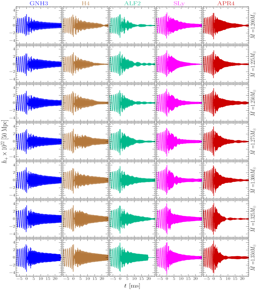
Figure 1: Gravitational waveforms for some of the cold-EOS binaries listed in Table. 1. The rows correspond to the gravitational masses, $\bar{M}=1.200,1.225,1.250,1.275,1.300,1.325,1350\,M_{\odot}$, respectively, while each column refers to a given EOS. The different EOSs are distinguished by different colours and we will adopt this colour-coding also for all the subsequent plots. All models have formed long-lived HMNSs with $t>20\,\mathrm{ms}$.

II.0.4 Gravitational-wave signal

The GW signal is extracted at different surfaces of constant coordinate radius using the Newman-Penrose formalism, so that the GW polarization amplitudes $h_{+}$ and $h_{\times}$ are related to Weyl curvature scalar $\psi_{4}$ by (see Sect. IV of Ref. Baiotti et al. (2008) for details)

$$\ddot{h}_{+}-{\rm i}\ddot{h}_{\times}=\psi_{4}=\sum_{\ell=2}^{\infty}\sum_{m=-\ell}^{\ell}\psi_{4}^{\ell m}\;{}_{-2}Y_{\ell m}(\theta,\varphi),$$ (5)

where the overdot indicates a time derivative and we have introduced the (multipolar) expansion of $\psi_{4}$ in spin-weighted spherical harmonics Goldberg et al. (1967) of spin-weight $s=-2$. In practice, all of our analysis is limited to the dominant mode, i.e., the $\ell=m=2$ mode

$$h_{+,\times}=\sum_{\ell=2}^{\infty}\sum_{m=-\ell}^{\ell}h^{\ell m}_{+,\times}\,{}_{-2}Y_{\ell m}\left(\theta,\varphi\right)\approx h^{22}_{+,\times}\,{}_{-2}Y_{22}\left(\theta,\varphi\right)\,,$$ (6)

where ${}_{s}Y_{\ell m}\left(\theta,\varphi\right)$ are the spin-weighted spherical harmonics. Following previous work Read et al. (2013); Takami et al. (2015), we align the waveforms at the “time of merger”, which we set to be $t=0$ and define to be correspondent to the time when the GW amplitude

$$|h|\equiv({h^{2}_{+}}+{h^{2}_{\times}})^{1/2}\,,$$ (7)

reaches its first maximum. As a result, for most binaries we consider GW signals in the time interval $t\in[-1500,5000]\,M_{\odot}\approx[-7.39,24.63]\,{\rm ms}$. After defining the instantaneous frequency of the GW as $f_{{}_{\mathrm{GW}}}\equiv\frac{1}{2\pi}(d\phi/dt)$, where $\phi=\arctan(h_{\times}/h_{+})$ is the phase of the complex gravitational waveform Read et al. (2013). The time of the merger is also used to define the “frequency at amplitude maximum” (or peak frequency in Ref. Read et al. (2013)) as $f_{\mathrm{max}}\equiv f_{{}_{\mathrm{GW}}}(t=0)$.

Another quantity used extensively in our analysis is the PSD of the effective amplitude and defined as

$$\tilde{h}(f)\equiv\sqrt{\frac{|\tilde{h}_{+}(f)|^{2}+|\tilde{h}_{\times}(f)|^{2}}{2}}\,,$$ (8)

with

$$\tilde{h}_{+,\times}(f)\equiv\left\{\begin{array}[]{ll}\displaystyle\int h_{+,\times}(t)\,e^{-i2\pi ft}dt&(f\geq 0)\\ \displaystyle 0&(f<0)\end{array}\right.\,,$$ (11)

and where the $+$ and $\times$ indices refer to the two polarization modes. Using this PSD, we can compute the signal-to-noise ratio (SNR) as

$$\mathrm{SNR}\equiv\left[~{}\int^{\infty}_{0}\frac{\bigl{|}2~{}\tilde{h}(f)f^{1/2}\bigr{|}^{2}}{S_{h}(f)}~{}\frac{df}{f}~{}\right]^{1/2}\,,$$ (12)

with $S_{h}(f)$ being the noise PSD of a given GW detector [e.g., Advanced LIGO url , or the Einstein Telescope (ET) Punturo et al. (2010a, b)].

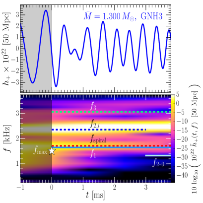
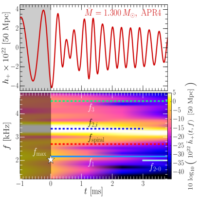
Figure 2: Two examples of the GW emission around the merger, i.e., $1\,{\rm ms}$ before the (gray-shaded area) and $4\,{\rm ms}$ after the merger. Both panels refer to a fiducial mass of $\bar{M}=1.300\,M_{\odot}$, with the left panel showing a representative stiff EOS (i.e., GNH3), while the right panel a representative soft EOS (i.e., APR4). The top part of each panel reports the gravitational strain $h_{+}$ for a source at $50\,{\rm Mpc}$, while the bottom part the corresponding spectrogram. Also marked with horizontal lines of different type and colour are the various frequencies discussed so far in the literature (see main text).

III Results

III.1 Waveform properties: transient signals

Figure 1 provides a summarising view of some of the waveforms (i.e., of $h_{+}$ for sources at a distance of $50\,{\rm Mpc}$) computed in this paper and that are combined with those of Takami et al. (2015) to offer a more comprehensive impression of the GW signal across different masses and EOSs. The figure is composed of 35 panels referring to the 35 equal-mass binaries with nuclear-physics EOSs that we have simulated and that have a postmerger signal of at least $20\,{\rm ms}$; binaries with shorter post-merger (e.g., ALF2-q10-M1400) and unequal-mass (e.g., GNH3-q09-M1300) are not reported in the figure but their properties are listed in Table 1. Different rows refer to models with the same mass, while different columns select the five cold EOSs considered and colour-coded for convenience. It is then rather easy to see how small differences across the various EOSs during the inspiral become marked differences after the merger. In particular, it is straightforward to observe how the GW signal increases considerably in frequency after the merger and how low-mass binaries with stiff EOSs (e.g., top-left panel for the GNH3 EOS) show a qualitatively different behaviour from high-mass binaries with soft EOSs (e.g., bottom-right panel for the APR4 EOS). Also quite apparent is that, independently of the mass considered, the post-merger amplitude depends sensitively on the stiffness of the EOS, with stiff EOSs (e.g., GNH3) yielding systematically larger amplitudes than soft EOSs (e.g., APR4).

What is less evident from Fig. 1 are the features of the transient GW signals emitted a few millisecond after the merger. To this scope, we present in Fig. 2 two representative examples that concentrate on a time window around the merger, i.e., one millisecond in the inspiral (light-gray shaded area) and four milliseconds after the merger. Both panels represent what could be the most realistic reference value for the mass, i.e., $\bar{M}=1.300\,M_{\odot}$, with the left panel referring to a representative soft EOS (i.e., GNH3), while the right panel showing the same but for a representative stiff EOS (i.e., APR4). The top part of each panel reports the gravitational strain $h_{+}$ for a source at $50\,{\rm Mpc}$, while the bottom part the corresponding spectrogram, i.e., the evolution of the PSD, where timeseries segments with length $\sim 8\,{\rm ms}$ and transformed with a Blackman window are overlapped by $90\%$. Also marked with horizontal line of different type and colour are the various frequencies that have been so far discussed in the literature when describing the spectral properties of the GW signal.

Although we have already mentioned such spectral properties in the Introduction, but we also briefly summarise them below:

• the frequencies $f_{\rm max}$ were first introduced in Ref. Read et al. (2013) and mark the instantaneous GW frequency at the merger, i.e., at GW amplitude maximum. These frequencies were discussed in Ref. Read et al. (2013), where they were first shown to correlate with the tidal deformability of the two stars; similar findings were later reported in Refs. Bernuzzi et al. (2014a); Takami et al. (2015). The values reported here are measured from the data (see also Fig. 7 below).

• the frequencies $f_{1},f_{2},f_{3}$ were introduced in Refs. Takami et al. (2014, 2015) and represent the three main peaks of the PSDs measured in those references. The frequencies were found to roughly follow the relation $f_{2}\simeq(f_{1}+f_{3})/2$, and a simple mechanical toy model was proposed in Takami et al. (2015) to explain simply this relation.

  

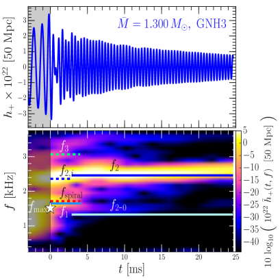
  Figure 3: The same as in Fig. 2, but shown on a much longer timescale, i.e., $25\,{\rm ms}$ after the merger. Note that all of the peaks present in the short transient stage (i.e., $t\lesssim 3\,{\rm ms}$) essentially disappear in the quasi-stationary evolution. The only exception is the $f_{2}$ peak, which slightly evolves from the $f_{2,i}$ frequency. In the case of a stiff EOS (e.g., for the H4 EOS, but not shown here) a trace of the $f_{2\mbox{-}0}$ mode is still present, although at very low amplitudes.

• the $f_{2}$ frequencies correspond to the $\ell=2=m$ fundamental mode of the HMNS and hence are equal to twice the rotation frequency of the bar deformation of the HMNS. Their values change slightly in time (by $\sim 5\%$), and we indicate with $f_{2,i}$ the values in the transient phase to distinguish them from the values $f_{2}$ attained in the subsequent quasi-stationary evolution of the GW signal.

• the values reported here for $f_{2,i},f_{2}$, and $f_{1}$ are measured from the data. In particular, the $f_{2,i}$ frequencies are measured from the spectrograms, while the $f_{2}$ frequencies from the full PSDs; see Sect. III.3). For the $f_{1}$ frequencies, instead, a first guess is predicted from the analytic expression Eq. (25) of Takami et al. (2015) [i.e., Eq. (20) here]; we then use these guesses and the spectrograms to refine the measured values of the $f_{1}$ frequencies, which we report in Figs. 2–6 and in Table 2. Such values of the $f_{1}$ frequencies are also used to obtain an improved estimate of the fitting coefficients (21). Finally, the third frequency is also predicted as $f_{3}=2f_{2,i}-f_{1}$.

• the frequencies $f_{2\mbox{-}0}$ were first introduced in Ref. Stergioulas et al. (2011) and refer to a coupling between the $\ell=2=m$ fundamental mode and a quasi-radial axisymmetric mode, i.e., with $m=0$, and that we indicate as $f_{m=0}$. The frequency of the latter mode can be measured, for instance, from the oscillations in the lapse function or the rest-mass density at the center of the HMNS Bauswein and Stergioulas (2015); Bauswein et al. (2016), so that $f_{2\mbox{-}0}\equiv f_{2}-f_{m=0}$ are effectively measured quantities.

• the frequencies $f_{\rm spiral}$ were first introduced in Ref. Bauswein and Stergioulas (2015) and refer to the contribution to the GW signal coming from a “rotating pattern of a deformation of spiral shape”. Because shapes in gauge-dependent quantities such as the rest-mass density are essentially impossible to measure in numerical-relativity calculations, we cannot measure these frequencies in our calculation. Hence, the values reported are those predicted from the analytic prescription given in Ref. Bauswein and Stergioulas (2015) [cf., Eq. (2) of Bauswein and Stergioulas (2015)]. It was also claimed that the $f_{\rm spiral}$ peak can be roughly reproduced in a toy model, but no details were given in Ref. Bauswein and Stergioulas (2015).

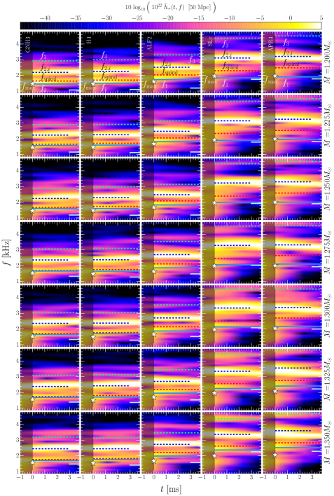
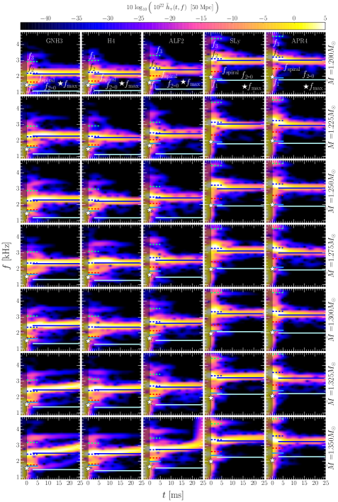
Figure 4: The left and right panels show short and long spectrograms similar to those presented in Figs. 2 and 3, but for the same set of binaries reported in Fig. 1.

The spectrograms in Fig. 2 contain a wealth of information about the transient post-merger phase. To clarify a series of imprecise and sometimes confusing statements recently appeared in the literature, we collect below the main information on the spectral properties of the transient. The points summarised below do not refer only to the models in Figs. 2 and 3, but to all of the models simulated [cf., Fig. 4].

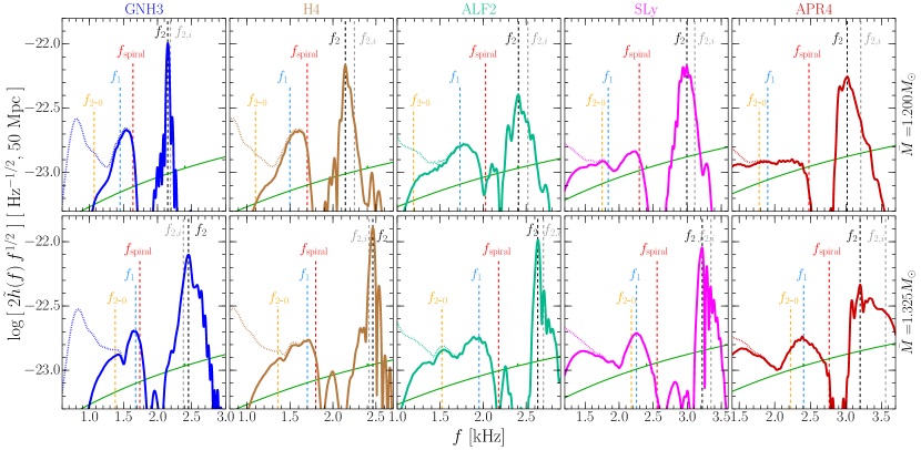
Figure 5: Total PSDs of the GW signals for all the EOSs considered and relative to a series of low-mass (i.e., $\bar{M}=1.200\,M_{\odot}$) and medium-mass binaries (i.e., $\bar{M}=1.325\,M_{\odot}$); these are the two masses also considered in Ref. Bauswein and Stergioulas (2015). The solid lines refer to the post-merger signal only, while the dotted lines report also the power during the short inspiral. Reported with vertical dashed lines of different colours are instead the values of the frequencies $f_{1}$, $f_{2,i}$, $f_{2}$, $f_{2\mbox{-}0}$, and $f_{\rm spiral}$. These are either measured from the PSDs or estimated numerically (see discussion in Sect. III.1). The PSDs are relative to GWs from binaries at a distance of $50\,{\rm Mpc}$ and we report also the sensitivity curves of Advanced LIGO as a reference (green line). Note that the $f_{1}$ and $f_{\rm spiral}$ frequencies (blue and red vertical dashed lines) are very similar for stiff EOSs (e.g., GNH3, H4), but significantly different for soft EOSs (e.g., SLy, APR4), making a proper distinction fallible. Note also that the $f_{2\mbox{-}0}$ frequencies (orange vertical dashed lines) do not always correspond to clearly identifiable peaks in the total PSDs.

• the frequencies $f_{2,i}$ (blue dashed lines) are short-lived and evolve into the $f_{2}$ frequencies as the GW signal reaches its quasi-stationary phase (i.e., the one after $t\simeq 3\,{\rm ms}$). This change is of the order of $\sim 5\%$, so that $f_{2}\sim(1\pm 0.05)\,f_{2,i}$.

• the frequencies $f_{1},f_{3}$ (light blue solid lines and green dashed lines) are instead short-lived and their amplitude becomes vanishingly small after the transient. This was remarked in Ref. Takami et al. (2015), where a simple toy model was developed to explain these frequencies as a result of the modulation of the (rotating) oscillation of the two stellar cores [cf., Appendix A of Takami et al. (2015)]. Note that although $f_{1},f_{3}$ are only predicted analytically, they do coincide with the maximum values of the spectrogram. This provides an important confirmation on the correctness of the interpretation in Ref. Takami et al. (2015).

• the frequencies $f_{2\mbox{-}0}$ (cyan solid lines) do not have significant power during the transient phase and it is only later that they may produce a contribution and only for rather stiff EOSs (cf., Fig. 4, which we discuss below). Note also that the frequencies $f_{2\mbox{-}0}$ are measured from $f_{2}$ and $f_{m=0}$, respectively, leaving no room for interpretation.

• the frequency $f_{\rm spiral}$ (red dashed lines) is essentially the same as the $f_{1}$ frequency for the stiff EOS GNH3, while it is significantly different for the soft EOS APR4. The fact that $f_{\rm spiral}\sim f_{1}$ in some cases but not in all cases, holds true also when considering other EOSs and was found also in Ref. Bauswein and Stergioulas (2015). We will touch on this point further below (see dashed blue and red lines in Figs. 5 and 6 and relative discussion).

• because the frequency $f_{\rm spiral}$ is predicted from an analytic expression [cf., Eq. (2) of Bauswein and Stergioulas (2015)], its coincidence with the $f_{1}$ frequency for stiff EOSs suggests that the two frequencies are just the same for stiff EOSs. On the other hand, for soft EOSs the frequencies $f_{\rm spiral}$ do select a genuinely different mode, which are however short-lived; as we will show in Fig. 5, the total power stored in these $f_{\rm spiral}$ modes is always very small in our data (see also Bauswein and Stergioulas (2015)).

• the only partial correspondence between the $f_{1}$ and $f_{\rm spiral}$ frequencies can explain why the $f_{1}$ frequencies are found to behave universally Takami et al. (2014, 2015), while the $f_{\rm spiral}$ are not Bauswein and Stergioulas (2015).

To recap, the analysis of the spectrograms in the transient phase reveals that three modes are clearly visible: $f_{2,i},f_{1},f_{3}$. The last two disappear later on, while the first one survives as $f_{2}$ and with changes of a few percent. The $f_{\rm spiral}$ frequencies essentially coincide with the $f_{1}$ frequencies for stiff EOSs, while marking a different mode for soft EOSs; these latter frequencies are short lived and provide a minimal contribution to the total PSD.

III.2 Waveform properties: quasi-stationary signals

We next discuss the spectral properties of the signal when considered over a much longer timescale, which we take to be at least $20\,{\rm ms}$ after the merger if the HMNS does not collapse before. This is shown in Fig. 3, again for two representative EOSs and for the fiducial mass of $\bar{M}=1.300\,M_{\odot}$. As anticipated in the previous Section, the only frequency surviving on these timescales is the $f_{2}$ peak (blue solid lines), which evolves slightly from the $f_{2,i}$ peak as the HMNS attains a quasi-stationary equilibrium. Other peaks, such those associated to $f_{1},f_{3},f_{\rm spiral}$ essentially vanish after the transient, while the $f_{2\mbox{-}0}$ peak retain only small powers.

Figure 4 is rather “dense”, but provides a comprehensive summary in terms of spectrograms of the results discussed in the last two sections. In particular, the left panel reports the spectrograms for the 35 binaries presented in Fig. 1, but concentrating on the transient phase, i.e., for $t\in[-1,4]\,{\rm ms}$, while the right panel shows the spectrograms for the complete GW signal. In essence, the two panels show that:

• for all the EOSs considered here, three frequencies appear in the transient phase: $f_{1},f_{2,i},f_{3}$.

• the $f_{\rm spiral}$ frequencies essentially coincide with the $f_{1}$ frequencies for stiff EOSs (i.e., GNH3, H4, and ALF2), but differ for soft EOSs (i.e., SLy and APR4).

• for soft EOSs, the $f_{\rm spiral}$ frequencies are systematically at larger frequencies than the $f_{1}$ frequencies (see, e.g., the model with $\bar{M}=1.225\,M_{\odot}$ for the APR4 EOS), but yield a very contribution to the overall PSD.

• after the transient, only the $f_{2}$ frequencies survive as an adjustment of the $f_{2,i}$ frequencies produced during the transient.

• the $f_{2\mbox{-}0}$ frequency can be easily measured from the oscillations of the lapse function but the associated power in the spectrograms is always extremely small and appreciable only after the transient and for a limited period of time (see, e.g., model with $\bar{M}=1.300-1.350\,M_{\odot}$ for stiff EOSs GNH3, H4 and ALF2).

III.3 Waveform properties: analysis of the full PSDs

The discussion has so far been focused on the analysis of the spectral properties of the GW signal as deduced when looking at the spectrograms. We next investigate how the spectral properties appear when analysing the full PSDs of the GW signal.

We start this discussion by considering two representative examples in Fig. 5, which reports the PSDs of a series of low-mass (i.e., $\bar{M}=1.200\,M_{\odot}$) and medium-mass binaries (i.e., $\bar{M}=1.325\,M_{\odot}$); solid lines refer to the post-merger signal only, while the dotted lines report also the power during the short inspiral. The frequencies relative to the peaks $f_{1}$, $f_{2,i}$, $f_{2}$, and $f_{2\mbox{-}0}$ are shown with vertical dashed lines of different colours. Additionally, the $f_{\rm spiral}$ frequency of Ref. Bauswein and Stergioulas (2015), which was reported for $\bar{M}=1.200,~{}1.350$ and $1.500\,M_{\odot}$ [cf., Eq. (2) of Bauswein and Stergioulas (2015)], are also shown as a reference. In essence, the PSDs in Fig. 5 reveal that:

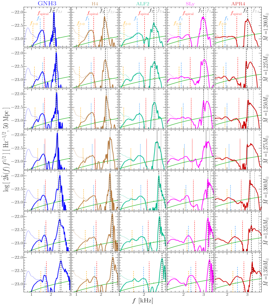
Figure 6: The same as in Fig. 5, but for the same set of binaries reported in Fig. 1. Note that the $f_{1}$ and $f_{\rm spiral}$ frequencies (blue and red vertical dashed lines) are very similar for stiff EOSs (e.g., GNH3, H4), but significantly different for soft EOSs (e.g., SLy, APR4).

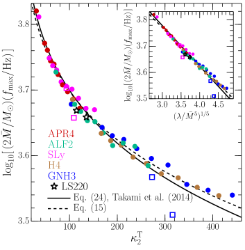
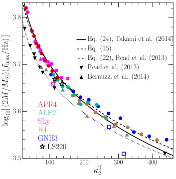
Figure 7: Left panel: Mass-weighted frequencies at amplitude maximum $f_{\mathrm{max}}$ shown as a function of the dimensionless tidal deformability $\kappa^{{}^{T}}_{2}$ (the inset shows the same data in terms of $(\lambda/\bar{M}^{5})^{1/5}$ to highlight the essentially linear behaviour). Filled circles of different colours refer to equal-mass binaries with different cold EOSs, the empty squares to the unequal-mass binaries, and the stars to the hot-EOS binariess. The black solid line shows the fit as given by Eq. (24) of Takami et al. (2015), while the black dashed line the fit with the updated coefficients (19). Right panel: The same as in the left panel but showing also the data from Refs. Read et al. (2013); Bernuzzi et al. (2014a), where a slightly different definition of the merger time is used and leads to the larger variance.

• for all the EOSs considered, the peak corresponding to the $f_{2}$ frequency is rather easy to recognise and is reasonably well reproduced by an analytic expression that we will discuss in Sect. III.4.

• the $f_{2,i}$ frequencies as measured from the spectrograms do not correspond to any visible peak in the total PSDs; this is to be expected given that these frequencies are only short lived and their contribution to the total PSD is much smaller than that of the $f_{2}$ frequencies.

• smaller but still clearly visible are the contributions of the $f_{1}$ and $f_{3}$ frequencies (the latter are not reported in Fig. 5 for clarity). This behaviour too is not surprising and is due to the short duration of these modes. Note that the $f_{1}$ frequencies in Fig. 5, which we recall are predicted analytically, also mark the presence of a local maximum in the PSD.

• for stiff EOSs, e.g., GNH4 and H4, the peaks corresponding to the $f_{1}$ and $f_{\rm spiral}$ frequencies are very similar, but they become distinct for soft EOSs, e.g., ALF2, SLy and APR4.

• when not being comparable to $f_{1}$, the $f_{\rm spiral}$ frequencies do not seem to mark any local maximum in the PSDs, see, for example the BNS with $\bar{M}=1.200\,M_{\odot}$ and the SLy EOS, or the BNS with $\bar{M}=1.350\,M_{\odot}$ and the EOSs SLy and APR4.

• the behaviour of the $f_{2\mbox{-}0}$ frequencies is far less clear. In those cases where it is comparable with the $f_{1}$ frequencies (e.g., for the SLy EOS), these frequencies can be associated to the same power excess attributed to the $f_{1}$ frequencies. In other cases, however, they are either associated to peaks with very limited power or are associated to peaks. This is not surprising since the $f_{2\mbox{-}0}$ peaks result from a mode coupling and are therefore expected to be less energetic.

The properties of the PSDs listed above and illustrated in Fig. 5 are not limited to the cases of the binary masses reported in that figure. This conclusion can be reached after inspecting Fig. 6, which is the same as Fig. 5, but reports also all the other masses considered. For compactness we do not report here the PSDs relative to the unequal-mass binaries considered, and whose PSDs show a very similar behaviour to the ones discussed so far.

III.4 Waveform properties: correlations with the stellar properties

In what follows we make use of the results discussed so far to correlate the spectral properties of the GW signal with the properties of the progenitor stellar models. As discussed extensively in Refs. Bauswein and Janka (2012); Bauswein et al. (2012); Read et al. (2013); Bernuzzi et al. (2014a); Takami et al. (2014, 2015); Bernuzzi et al. (2015b), some of these correlations appear to be “universal”, i.e., only slightly dependent on the EOS, and can therefore be used to constrain the physical properties of the progenitor stars and hence the EOS.

III.4.1 Inspiral and merger

We start by considering the inspiral part of the signal. Figure 7 reports the mass-weighted frequencies at amplitude maximum $f_{\mathrm{max}}$ as a function of the tidal polarizability parameter $\kappa_{2}^{{}^{T}}$ for a generic unequal-mass binary. We recall that the latter is defined as (see, e.g., Bernuzzi et al. (2014a))

$$\kappa_{2}^{{}^{T}}\equiv 2\left[q\left(\frac{X_{{}_{A}}}{C_{{}_{A}}}\right)^{5}k^{{}^{A}}_{2}+\frac{1}{q}\left(\frac{X_{{}_{B}}}{C_{{}_{B}}}\right)^{5}k^{{}^{B}}_{2}\right]\,,$$ (13)

where $A$ and $B$ refer to the primary and secondary stars in the binary

$$q\equiv\frac{M_{{}_{B}}}{M_{{}_{A}}}\leq 1\,, X_{{}_{A,B}}\equiv\frac{M_{{}_{A,B}}}{M_{{}_{A}}+M_{{}_{B}}}\,,$$ (14)

$k_{2}^{{}^{A,B}}$ are the $\ell=2$ dimensionless tidal Love numbers, and $\mathcal{C}_{{}_{A,B}}\equiv M_{{}_{A,B}}/R_{{}_{A,B}}$ are the compactnesses. In the case of equal-mass binaries, $k_{2}^{A}=k_{2}^{B}=\bar{k}_{2}$, and expression (13) reduces to

$$\kappa_{2}^{{}^{T}}\equiv\frac{1}{8}\bar{k}_{2}\left(\frac{\bar{R}}{\bar{M}}\right)^{5}=\frac{3}{16}\Lambda=\frac{3}{16}\frac{\lambda}{\bar{M}^{5}}\,,$$ (15)

where the quantity

$$\lambda\equiv\frac{2}{3}\bar{k}_{2}{\bar{R}}^{5}\,.$$ (16)

is another commonly employed way of expressing the tidal Love number for equal-mass binaries Read et al. (2013), while $\Lambda\equiv\lambda/\bar{M}^{5}$ is its dimensionless counterpart and was employed in Takami et al. (2015).

The black solid line in the left panel of Fig. 7 shows the fit as given by Eq. (24) of Takami et al. (2015), where five realistic EOSs (i.e., APR4, ALF2, SLy, H4, GNH3) and an ideal-fluid EOS with $\Gamma=2$ were employed across a range of five different masses for each EOS. Such a fit was expressed as [cf., Eq. (24) of Takami et al. (2015)]

$$\log_{10}\left(\frac{f_{\mathrm{max}}}{\mathrm{kHz}}\right)\approx a_{0}+a_{1}\,\left(\kappa^{{}^{T}}_{2}\right)^{\!\!1/5}\!-\log_{10}\left(\frac{2\bar{M}}{M_{\odot}}\right)\,,$$ (17)

where

$$a_{0}=4.242\,, a_{1}=-0.216\,.$$ (18)

Making use of the larger sample of binaries and excluding from the fit the ideal-fluid EOS, we can further refine the fit and obtain new and slightly modified coefficients

$$a_{0}=4.186\,, a_{1}=-0.195\,.$$ (19)

The new fit is indicated with a black dashed in the left panel of Fig. 7, which also reports in an inset the same data but when represented via the dimensionless tidal deformability $(\lambda/M^{5})^{1/5}$ to highlight the essentially linear dependence in terms of this variable.

In the right panel of Fig. 7, we instead show the same correlation as in the left panel (and the corresponding fitting expressions) but when using the data taken from Refs. Read et al. (2013); Bernuzzi et al. (2014a). Note that in these cases, the frequencies reported are measured at the peak of amplitude of one of the polarization modes of the strain, i.e., at the maximum amplitude of $h^{2}_{+}(t)$ rather than of $h(t)\equiv\left(h^{2}_{+}+h^{2}_{\times}\right)^{1/2}$; we believe this slight differences is responsible for the larger variance in the correlation (see discussion in Sect. V C. in Takami et al. (2015)).

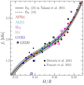
Figure 8: Left panel: Values of the low-frequency peaks $f_{1}$ for equal-mass binaries (we use the same symbol convention as in Fig. 7) shown as a function of the average stellar compactness. The solid black line shows the quasi-universal relation first reported in Takami et al. (2015). Note that the new data, including the low- and high-mass models (e.g., $\bar{M}=1.200,1.500\,M_{\odot}$), respect the “universal” behaviour. Also reported is the data presented in Ref. Dietrich et al. (2015) (black diamonds) and Foucart et al. (2016) (black triangles). Right panel: The same data as in the left panel, but shown as a function of the dimensionless tidal deformability $\kappa^{{}^{T}}_{2}$ and highlighting a quasi-universal relation also in terms of this quantity.

Overall, the data reported in Fig. 7 confirms what was first pointed out in Ref. Read et al. (2013), namely, that a rather tight “universal” correlation exists between the frequency at peak amplitude and the tidal deformability; for equal-mass binaries, the largest difference between the values measured for $f_{\rm max}$ and those predicted by the fit are $\simeq 3.6\%$, but the average deviation is much smaller and $\simeq 1.3\%$ only.

The correlation becomes weaker when considering unequal-mass binaries and this is clearly shown by the data marked with empty squares at $\kappa^{{}^{T}}_{2}\simeq 105$ and at $\kappa^{{}^{T}}_{2}\simeq 315$. Both points refer respectively to the APR4 and GNH3 binaries with the smallest mass ratio of $q\simeq 0.8$ and this can be interpreted as the “breaking” of the universality for small (and possibly unrealistic) mass ratios. Given that the dynamics and GW signal in these cases is rather different from the corresponding equal-mass binaries (the merger necessarily happens at lower frequencies as the tidal interaction is amplified and the lower-mass star disrupted), this is perfectly plausible; however additional simulations will be needed to confirm this conjecture.

III.4.2 Post-merger

Next, we consider the correlations in the post-merger part of the signal and concentrate initially on the low-frequency $f_{1}$ peaks. The left panel of Fig. 8 reports the values of such frequencies as a function of the stellar compactness. The solid black line represents the “universal” relation first reported in Ref. Takami et al. (2015) and expressed as a cubic polynomial [cf., Eq. (25) of Ref. Takami et al. (2015)]

$$f_{1}\approx b_{0}+b_{1}~{}{\mathcal{C}}+b_{2}~{}{\mathcal{C}}^{2}+b_{3}~{}{\mathcal{C}}^{3}\ {\mathrm{kHz}}\,,$$ (20)

where the fitting coefficients given by Takami et al. (2015) have been further refined after using the larger sample of data considered here and are given by

$$b_{0}=-35.17\,, b_{1}=727.99\,,$$

$$b_{2}=-4858.54\,, b_{3}=10989.88\,.$$ (21)

Also indicated with a gray shaded band is the overall $\lesssim 0.06\,{\rm kHz}$ uncertainty in the fit related either to the truncation error or to the determination of the frequencies Takami et al. (2015).

Note that the data relative to the new binaries is in full agreement with our previous results in Takami et al. (2015) and that even the very low-mass binaries, i.e., with $\bar{M}=1.200\,M_{\odot}$, support the universal relation. Hence, we believe that the mismatch found in Bauswein and Stergioulas (2015) is due to the incorrect association of the $f_{1}$ frequency with the $f_{\rm spiral}$ frequencies.

Also reported in the figure are the putative $f_{1}$ frequencies as taken from Refs. Dietrich et al. (2015); Foucart et al. (2016), respectively for binaries with $\bar{M}=1.350\,M_{\odot}$ and $q=0.862$ and $q=1$, evolved with EOSs MS1, H4, ALF2, and SLy Dietrich et al. (2015), as well as for binaries with $\bar{M}=1.200\,M_{\odot}$ and $q=1$ evolved with EOSs LS220, DD2, and SFHo Foucart et al. (2016). In particular, in the case of the SFHo EOS, we believe that the value reported in Table II of Foucart et al. (2016) (i.e., $2.1\,{\rm kHz}$) actually refers to the $f_{\rm spiral}$ frequency and that the correct value for the $f_{1}$ frequency is the low-frequency one which is clearly marked in the left panel of Fig. 6 in Foucart et al. (2016) (i.e., $1.7\,{\rm kHz}$). We have already remarked that in the case of soft EOSs and low-mass binaries it is very easy to confuse the $f_{1}$ frequency with the $f_{\rm spiral}$ one; we believe this is one of those instances. Indeed, when this correction is made, all of the data of Refs. Dietrich et al. (2015) and Foucart et al. (2016) appears in good agreement with the expected “universal” behaviour and its variance.

The $f_{1}$ frequencies also show a very good tight correlation with the the tidal deformability. This was already reported in Ref. Takami et al. (2015) (cf., Fig. 15 of Takami et al. (2015)) and we further remark on this point in the right panel of Fig. 8, where we employ the same data of the left panel and fit it with a third-order polynomial expansion of the dimensionless tidal deformability $(\kappa^{{}^{T}}_{2})^{1/5}$

$$f_{1}\approx c_{0}+c_{1}~{}\left(\kappa^{{}^{T}}_{2}\right)^{\!\!1/5}+c_{2}~{}\left(\kappa^{{}^{T}}_{2}\right)^{2/5}+c_{3}~{}\left(\kappa^{{}^{T}}_{2}\right)^{3/5}\ {\mathrm{kHz}}\,,$$ (22)

with the coefficients being given by

$$c_{0}=45.195\,, c_{1}=-43.484\,,$$

$$c_{2}=14.653\,, c_{3}=-1.6623\,.$$ (23)

When considering only equal-mass binaries, the largest deviation from the fit (22) is $\simeq{7.1}\%$, while the average is only $\simeq{2.3}\%$.

We next consider the correlations of the $f_{2,i}$ and $f_{2}$ frequencies with the stellar properties. We recall that the $f_{2,i}$ and $f_{2}$ frequencies correspond to the same fundamental $\ell=2=m$ mode of oscillation and the different denomination refers to whether the frequencies are measured during the transient phase ($f_{2,i}$) or in the quasi-periodic one ($f_{2}$). These frequencies are reported as a function of the dimensionless tidal deformability in the left panel Fig. 9, where we report the data taken from all of our simulations, including those that produce a black hole before 25 ms; a similar figure was presented in Ref. Takami et al. (2015) (cf., Fig. 15 of Takami et al. (2015)), but here we also provide a fitting function in terms of the dimensionless tidal deformability, both for the $f_{2}$ and the $f_{2,i}$ frequencies (see inset in the left panel of Fig. 9) as

$$f_{2,i} \approx 6.401-1.299\,\left(\kappa^{{}^{T}}_{2}\right)^{\!\!1/5}\quad\mathrm{kHz}\,,$$ (24)

$$f_{2} \approx 5.832-1.118\,\left(\kappa^{{}^{T}}_{2}\right)^{\!\!1/5}\quad\mathrm{kHz}\,.$$ (25)

Relative to the equal-mass binaries, the largest (average) deviations from the fit are $\simeq 11\%\ (4.9\%)$ for the $f_{2,i}$ frequencies and $\simeq 9.0\%\ (3.0\%)$ for the $f_{2}$ frequencies.

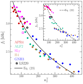
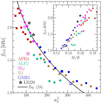
Figure 9: Left panel: Values of the $f_{2}$ peak frequencies shown as a function of the dimensionless tidal deformability $\kappa^{{}^{T}}_{2}$ (we use the same symbol convention as in Fig. 7). Although there is a correlation, the scatter is much larger than for the $f_{\rm max}$ or $f_{1}$ frequencies (see Figs. 7 and 8). The inset shows instead the $f_{2,i}$ frequencies for which the scatter is larger. Right panel: Values of the $f_{2\mbox{-}0}$ peak frequencies shown as a function of the dimensionless tidal deformability $\kappa^{{}^{T}}_{2}$. In the inset, instead, the frequencies are reported as a function of the average compactness $\bar{M}/\bar{R}$, as done in Ref. Bauswein and Stergioulas (2015).

In addition, we present in the right panel of Fig. 9 the correlation between the $f_{2\mbox{-}0}$ frequencies and the tidal deformability. We recall that the $f_{2\mbox{-}0}$ frequencies are simply the difference between the $f_{2}$ frequencies, which are easy to measure from the PSDs and the $f_{m=0}$ frequencies that can be estimated from the analysis of the data of the simulations (e.g., via the oscillation frequencies of the central rest-mass density or of the lapse function). In this sense, the $f_{2\mbox{-}0}$ frequencies are straightforward to compute; yet, as discussed above, these do not always correspond to a clearly visible peak in the total PSDs (cf., Fig. 6). Using all of this data we obtain a linear fit in terms of shown as a black solid line

$$f_{2\mbox{-}0} \approx 5.424-1.350\,\left(\kappa^{{}^{T}}_{2}\right)^{\!\!1/5}\quad\mathrm{kHz}\,.$$ (26)

A similar correlation is exhibited by the compactness (see Bauswein and Stergioulas (2015) and also the inset in the right panel of Fig. 9) and this is not particularly surprising given the fundamental nature of the $f_{2\mbox{-}0}$ frequencies. Because the correlation is weaker, the maximum and average deviations from the fit are of $\simeq 36\%$ and $\simeq 8.3\%$, respectively.

We conclude this Section by reporting the fitting expressions for the $f_{\rm spiral}$ frequencies as given by Eq. (2) in Bauswein and Stergioulas (2015) for equal-mass binaries with $\bar{M}=1.350\,M_{\odot}$,

$$f_{\rm spiral}\approx 6.16-82.1~{}{\mathcal{C}}+358~{}{\mathcal{C}}^{2}\quad{\mathrm{kHz}}\,.$$ (27)

No fitting expression was provided in Bauswein and Stergioulas (2015) for the binaries with $\bar{M}=1.200,1.500\,M_{\odot}$, but it was not difficult to reconstruct the behaviour of $f_{\rm spiral}$ through a quadratic two-dimensional fit in terms of the compactness and average gravitational mass of the binary, i.e.,

$$f_{\rm spiral}\approx ~{}d_{0}+d_{1}~{}{\mathcal{C}}+d_{2}~{}{\mathcal{C}}^{2}+$$

$$~{}d_{3}~{}\bar{M}+d_{4}~{}\bar{M}^{2}+d_{5}~{}{\mathcal{C}}~{}\bar{M}\quad\mathrm{kHz}\,,$$ (28)

and where

$$d_{0}=3.28\,, d_{1}=-8.68\,, d_{2}=174\,,$$

$$d_{3}=-2.34\,, d_{4}=0.99\,, d_{5}=-13.0\,.$$ (29)

Expression (III.4.2) is the one used when indicating the expected $f_{\rm spiral}$ frequencies in all the figures of this paper; a comparison of the two-dimensional fit (III.4.2) with the various fits suggested by Ref. Bauswein and Stergioulas (2015) will be presented in Appendix C.

IV Conclusions

The merger of a neutron-star binary is expected to be accompanied not only by a highly energetic electromagnetic signal, but also by a strong signal in GWs that will contain important signatures of the EOS of matter at nuclear densities. These signatures are contained both in the inspiral and in the post-merger signals and, following previous work of a number of authors Baiotti et al. (2010); Bernuzzi et al. (2012b); Radice et al. (2014a, b, 2015); Hotokezaka et al. (2016); Read et al. (2013); Bauswein and Janka (2012); Stergioulas et al. (2011); Bauswein et al. (2012); Hotokezaka et al. (2013); Bauswein et al. (2014); Takami et al. (2014, 2015); Bernuzzi et al. (2015b); Palenzuela et al. (2015); Bauswein and Stergioulas (2015); Dietrich et al. (2015); Foucart et al. (2016) we have here analysed the GW signal from merging neutron star binaries.

A particularly important goal of this work has been the analysis of the post-merger signal, which presents a number of quite strong spectral features that, just like spectral lines from the atmospheres of normal stars, can be used to extract information on the physical properties of the progenitor neutron stars. More specifically, we have tried to clarify whether or not some of these spectral features can be correlated with the properties of the stars before the merger in a way that is quasi-universal, that is, only weakly dependent on the EOS.

To this scope we have simulated a large number of neutron-star binaries in full general relativity and relativistic hydrodynamics. The binaries, which are mostly with equal masses, have total masses as low as $2.4\,M_{\odot}$ and as large as $3.0\,M_{\odot}$, spanning six different nuclear-physics EOSs. Because of the close similarities in the EOSs, the new set of binaries has been analysed together with the one already presented in Refs. Takami et al. (2014, 2015), thus providing a total sample of 56 binaries, arguably the largest studied to date in general relativity and with nuclear-physics EOSs.

A systematic analysis of the complete sample has allowed us to obtain a rather robust picture of the spectral properties of the GW signal and hopefully clarify a number of aspects that have been debated recently in the literature. In essence, our most important findings can be summarised as follows:

• the instantaneous GW frequency when the amplitude reaches its first maximum is related quasi-universally with the tidal deformability of the two stars.

• this correlation is observed for binaries with masses that do not differ of more than $20\%$.

• the spectral properties vary during the post-merger phase with a marked difference between a transient phase lasting a few millisecond after the merger and a following quasi-stationary phase.

• the most robust features of the post-merger signal pertain four frequencies: $f_{1},f_{2},f_{3}$, and $f_{2\mbox{-}0}$, where $f_{2}\simeq(f_{1}+f_{3})/2$ and $f_{2\mbox{-}0}$ is the result of a mode coupling.

• when distinguishing the spectral peaks between these two phases, a number of ambiguities in the identification of the peaks disappear, leaving a rather simple and robust picture.

• “universal” relations are found between the spectral features and the physical properties of the neutron stars.

• for all of the correlations between the spectral features and the stellar properties, simple analytic expressions can be found either in terms of the dimensionless tidal deformability or of the stellar compactness.

When considered as a whole and in the light of recent direct detection of GWs Abbott et al. (2016), these results open the exciting and realistic prospects of constraining the EOS of nuclear matter via GW observations of merging BNSs. At the same time, the robustness of these results needs to be validated when different physical conditions are assumed for the merging neutron stars. These include accounting a nonzero amount of initial stellar spin Kastaun et al. (2013); Tsatsin and Marronetti (2013); Bernuzzi et al. (2014b); Tsokaros et al. (2015); Kastaun and Galeazzi (2015), evaluating the modifications introduced by ideal- and resistive-MHD effects Giacomazzo et al. (2011); Dionysopoulou et al. (2015), and assessing the impact that the $m=1$ shear instability Ou and Tohline (2006); Corvino et al. (2010); Anderson et al. (2008b); East et al. (2016) may have on the post-merger spectrum when the instability is able to fully develop and persist on secular timescales. Furthermore, while some examples of unequal-mass binaries or of genuinely three-dimensional EOSs have been considered here, a more systematic analysis needs to be performed; this will be part of our future work.

Appendix A Summary of stellar properties

We report in Table 1 a summary of the main physical properties of the binaries simulated in this work; some of the data has already been provided in Ref. Takami et al. (2015), but we report it also here for completeness. The various columns denote the gravitational mass ratio $q\equiv M_{{}_{B}}/M_{{}_{A}}$ at infinite separation, the average gravitational mass $\bar{M}$ at infinite separation, the average radius $\bar{R}$ at infinite separation, the ADM mass $M_{\mathrm{ADM}}$ of the system at initial separation, the baryon mass $\bar{M}_{\mathrm{b}}$, the compactness ${\mathcal{C}}$, the orbital frequency $f_{\mathrm{orb}}$ at the initial separation, the total angular momentum $J$ at the initial separation, the dimensionless moment of inertia $\bar{I}/\bar{M}^{3}$ at infinite separation (which is tightly correlated with the compactness Breu and Rezzolla (2016)), the $\ell=2$ dimensionless tidal Love number $\bar{k}_{2}$ at infinite separation, the dimensionless tidal deformability $\lambda/\bar{M}^{5}$, and the contact frequency $f_{\rm cont}$. All quantities with a bar are defined as averages, i.e., $\bar{\Psi}\equiv(\Psi_{{}_{A}}+\Psi_{{}_{B}})/2$.

model	EOS	$q$	$\bar{M}$	$\bar{R}$	$M_{\mathrm{ADM}}$	$\bar{M_{\mathrm{b}}}$	$\bar{M}/\bar{R}$	$f_{\mathrm{orb}}$	$J$	$J/M_{\mathrm{ADM}}^{2}$	$\bar{I}/\bar{M}^{3}$	$\bar{k_{2}}$	$\lambda/\bar{M}^{5}$	$f_{\rm cont}$
			$[M_{\odot}]$	$[\mathrm{km}]$	$[M_{\odot}]$	$[M_{\odot}]$		$[\mathrm{Hz}]$	$[M_{\odot}^{2}]$				$[\mathrm{Hz}]$
GNH3-q10-M1200	GNH3	$1.000$	$1.200$	$13.827$	$2.3796$	$1.2882$	$0.12814$	$268.89$	$5.9899$	$1.0579$	$20.298$	$0.12184$	$2351.1$	$1235.2$
GNH3-q10-M1225	GNH3	$1.000$	$1.225$	$13.823$	$2.4288$	$1.3172$	$0.13085$	$2.7111$	$6.1967$	$1.0505$	$19.575$	$0.11970$	$2080.2$	$1248.6$
GNH3-q10-M1250	GNH3	$1.000$	$1.250$	$13.817$	$2.4780$	$1.3464$	$0.13358$	$273.29$	$6.4067$	$1.0434$	$18.890$	$0.11753$	$1842.4$	$1262.1$
GNH3-q10-M1275	GNH3	$1.000$	$1.275$	$13.810$	$2.5271$	$1.3756$	$0.13632$	$275.38$	$6.6187$	$1.0364$	$18.237$	$0.11531$	$1633.0$	$1275.7$
GNH3-q10-M1300	GNH3	$1.000$	$1.300$	$13.801$	$2.5763$	$1.4050$	$0.13908$	$277.44$	$6.8340$	$1.0296$	$17.614$	$0.11305$	$1448.1$	$1289.4$
GNH3-q10-M1325	GNH3	$1.000$	$1.325$	$13.790$	$2.6255$	$1.4345$	$0.14187$	$279.53$	$7.0538$	$1.0233$	$17.019$	$0.11075$	$1284.7$	$1303.2$
GNH3-q10-M1350	GNH3	$1.000$	$1.350$	$13.777$	$2.6746$	$1.4641$	$0.14468$	$281.58$	$7.2766$	$1.0172$	$16.450$	$0.10841$	$1139.9$	$1317.3$
GNH3-q10-M1375	GNH3	$1.000$	$1.375$	$13.762$	$2.7237$	$1.4938$	$0.14753$	$283.58$	$7.5023$	$1.0113$	$15.904$	$0.10602$	$1011.5$	$1331.7$
GNH3-q10-M1400	GNH3	$1.000$	$1.400$	$13.744$	$2.7729$	$1.5236$	$0.15040$	$285.56$	$7.7311$	$1.0055$	$15.381$	$0.10359$	$897.44$	$1346.3$
GNH3-q10-M1500	GNH3	$1.000$	$1.500$	$13.648$	$2.9692$	$1.6442$	$0.16228$	$293.15$	$8.6778$	$0.9843$	$13.479$	$0.09347$	$553.71$	$1408.3$
GNH3-q09-M1300	GNH3	$0.926$	$1.300$	$13.797$	$2.5763$	$1.4052$	$0.13912$	$277.51$	$6.8255$	$1.0283$	$17.607$	$0.11297$	$1445.0$	$1289.9$
GNH3-q08-M1275	GNH3	$0.821$	$1.275$	$13.789$	$2.5274$	$1.3770$	$0.13653$	$275.37$	$6.5564$	$1.0264$	$18.205$	$0.11483$	$1613.6$	$1278.6$
H4-q10-M1200	H4	$1.000$	$1.200$	$13.516$	$2.3796$	$1.2922$	$0.13109$	$268.83$	$5.9885$	$1.0576$	$19.918$	$0.12779$	$2200.9$	$1278.1$
H4-q10-M1225	H4	$1.000$	$1.225$	$13.525$	$2.4288$	$1.3213$	$0.13373$	$271.05$	$6.1956$	$1.0503$	$19.247$	$0.12571$	$1959.3$	$1290.1$
H4-q10-M1250	H4	$1.000$	$1.250$	$13.533$	$2.4780$	$1.3506$	$0.13638$	$273.25$	$6.4058$	$1.0432$	$18.610$	$0.12361$	$1746.5$	$1302.1$
H4-q10-M1275	H4	$1.000$	$1.275$	$13.539$	$2.5271$	$1.3799$	$0.13904$	$275.40$	$6.6191$	$1.0364$	$18.004$	$0.12147$	$1558.3$	$1314.1$
H4-q10-M1300	H4	$1.000$	$1.300$	$13.544$	$2.5763$	$1.4094$	$0.14172$	$277.52$	$6.8356$	$1.0299$	$17.426$	$0.11930$	$1391.4$	$1326.1$
H4-q10-M1325	H4	$1.000$	$1.325$	$13.548$	$2.6255$	$1.4390$	$0.14440$	$279.60$	$7.0552$	$1.0235$	$16.873$	$0.11708$	$1243.1$	$1338.3$
H4-q10-M1350	H4	$1.000$	$1.350$	$13.550$	$2.6746$	$1.4687$	$0.14711$	$281.61$	$7.2770$	$1.0173$	$16.344$	$0.11483$	$1111.1$	$1350.6$
H4-q10-M1375	H4	$1.000$	$1.375$	$13.550$	$2.7237$	$1.4985$	$0.14983$	$283.55$	$7.5010$	$1.0111$	$15.837$	$0.11253$	$993.41$	$1363.1$
H4-q10-M1400	H4	$1.000$	$1.400$	$13.548$	$2.7728$	$1.5284$	$0.15258$	$285.50$	$7.7293$	$1.0053$	$15.350$	$0.11019$	$888.32$	$1375.7$
H4-q10-M1500	H4	$1.000$	$1.500$	$13.518$	$2.9692$	$1.6494$	$0.16384$	$293.13$	$8.6772$	$0.9842$	$13.580$	$0.10046$	$567.34$	$1428.7$
ALF2-q10-M1200	ALF2	$1.000$	$1.200$	$12.227$	$2.3795$	$1.3076$	$0.14491$	$268.76$	$5.9850$	$1.0570$	$17.519$	$0.13524$	$1410.9$	$1485.5$
ALF2-q10-M1225	ALF2	$1.000$	$1.225$	$12.252$	$2.4288$	$1.3373$	$0.14762$	$271.00$	$6.1923$	$1.0497$	$16.975$	$0.13290$	$1263.8$	$1496.2$
ALF2-q10-M1250	ALF2	$1.000$	$1.250$	$12.276$	$2.4779$	$1.3672$	$0.15034$	$273.16$	$6.4014$	$1.0425$	$16.455$	$0.13049$	$1132.6$	$1507.0$
ALF2-q10-M1275	ALF2	$1.000$	$1.275$	$12.298$	$2.5271$	$1.3971$	$0.15307$	$275.12$	$6.6103$	$1.0351$	$15.957$	$0.12803$	$1015.6$	$1517.9$
ALF2-q10-M1300	ALF2	$1.000$	$1.300$	$12.319$	$2.5763$	$1.4272$	$0.15582$	$277.26$	$6.8274$	$1.0287$	$15.480$	$0.12552$	$911.00$	$1529.0$
ALF2-q10-M1325	ALF2	$1.000$	$1.325$	$12.337$	$2.6254$	$1.4574$	$0.15858$	$279.36$	$7.0475$	$1.0224$	$15.021$	$0.12297$	$817.44$	$1540.1$
ALF2-q10-M1350	ALF2	$1.000$	$1.350$	$12.353$	$2.6746$	$1.4877$	$0.16136$	$281.42$	$7.2708$	$1.0164$	$14.581$	$0.12037$	$733.63$	$1551.5$
ALF2-q10-M1375	ALF2	$1.000$	$1.375$	$12.368$	$2.7237$	$1.5181$	$0.16415$	$283.45$	$7.4970$	$1.0106$	$14.158$	$0.11773$	$658.50$	$1563.0$
ALF2-q10-M1400	ALF2	$1.000$	$1.400$	$12.380$	$2.7728$	$1.5487$	$0.16697$	$285.44$	$7.7266$	$1.0049$	$13.750$	$0.11505$	$591.07$	$1574.8$
ALF2-q10-M1500	ALF2	$1.000$	$1.500$	$12.409$	$2.9692$	$1.6723$	$0.17847$	$293.14$	$8.6758$	$0.9841$	$12.261$	$0.10404$	$383.01$	$1624.3$
SLy-q10-M1200	SLy	$1.000$	$1.200$	$11.465$	$2.3795$	$1.3116$	$0.15454$	$268.59$	$5.9804$	$1.0562$	$14.981$	$0.10746$	$812.79$	$1636.0$
SLy-q10-M1225	SLy	$1.000$	$1.225$	$11.468$	$2.4287$	$1.3417$	$0.15772$	$2.7084$	$6.1874$	$1.0489$	$14.478$	$0.10507$	$717.63$	$1652.4$
SLy-q10-M1250	SLy	$1.000$	$1.250$	$11.469$	$2.4779$	$1.3720$	$0.16092$	$273.04$	$6.3977$	$1.0420$	$14.000$	$0.10266$	$634.27$	$1668.8$
SLy-q10-M1275	SLy	$1.000$	$1.275$	$11.470$	$2.5271$	$1.4024$	$0.16413$	$275.20$	$6.6110$	$1.0352$	$13.545$	$0.10025$	$561.11$	$1685.3$
SLy-q10-M1300	SLy	$1.000$	$1.300$	$11.469$	$2.5763$	$1.4330$	$0.16736$	$277.34$	$6.8275$	$1.0287$	$13.113$	$0.097835$	$496.81$	$1701.9$
SLy-q10-M1325	SLy	$1.000$	$1.325$	$11.468$	$2.6254$	$1.4637$	$0.17060$	$279.36$	$7.0455$	$1.0221$	$12.702$	$0.095415$	$440.20$	$1718.5$
SLy-q10-M1350	SLy	$1.000$	$1.350$	$11.465$	$2.6745$	$1.4946$	$0.17386$	$281.34$	$7.2663$	$1.0158$	$12.309$	$0.092993$	$390.29$	$1735.2$
SLy-q10-M1375	SLy	$1.000$	$1.375$	$11.461$	$2.7237$	$1.5256$	$0.17714$	$283.37$	$7.4923$	$1.0100$	$11.935$	$0.090570$	$346.23$	$1752.1$
SLy-q10-M1400	SLy	$1.000$	$1.400$	$11.456$	$2.7728$	$1.5568$	$0.18043$	$285.36$	$7.7215$	$1.0043$	$11.577$	$0.088149$	$307.28$	$1769.1$
SLy-q10-M1500	SLy	$1.000$	$1.500$	$11.424$	$2.9692$	$1.6832$	$0.19387$	$293.05$	$8.6705$	$0.9835$	$10.292$	$0.007850$	$191.10$	$1838.9$
SLy-q09-M1300	SLy	$0.926$	$1.300$	$11.467$	$2.5763$	$1.4333$	$0.16739$	$277.23$	$6.8154$	$1.0268$	$13.115$	$0.097828$	$496.31$	$1702.3$
SLy-q08-M1275	SLy	$0.821$	$1.275$	$11.457$	$2.5273$	$1.4043$	$0.16432$	$275.08$	$6.5460$	$1.0249$	$13.560$	$0.10018$	$557.53$	$1688.2$
APR4-q10-M1200	APR4	$1.000$	$1.200$	$11.034$	$2.3795$	$1.3173$	$0.16058$	$268.60$	$5.9801$	$1.0562$	$14.100$	$0.10415$	$650.23$	$1732.9$
APR4-q10-M1225	APR4	$1.000$	$1.225$	$11.043$	$2.4287$	$1.3478$	$0.16379$	$270.85$	$6.1870$	$1.0489$	$13.651$	$0.10197$	$576.72$	$1748.6$
APR4-q10-M1250	APR4	$1.000$	$1.250$	$11.052$	$2.4779$	$1.3783$	$0.16700$	$273.05$	$6.3973$	$1.0419$	$13.226$	$0.099787$	$512.14$	$1764.3$
APR4-q10-M1275	APR4	$1.000$	$1.275$	$11.060$	$2.5271$	$1.4090$	$0.17022$	$275.22$	$6.6107$	$1.0351$	$12.821$	$0.097595$	$455.30$	$1779.9$
APR4-q10-M1300	APR4	$1.000$	$1.300$	$11.067$	$2.5763$	$1.4399$	$0.17344$	$277.24$	$6.8245$	$1.0282$	$12.436$	$0.095396$	$405.19$	$1795.5$
APR4-q10-M1325	APR4	$1.000$	$1.325$	$11.073$	$2.6254$	$1.4709$	$0.17667$	$279.31$	$7.0437$	$1.0219$	$12.070$	$0.093194$	$360.93$	$1811.1$
APR4-q10-M1350	APR4	$1.000$	$1.350$	$11.079$	$2.6746$	$1.5020$	$0.17992$	$281.37$	$7.2665$	$1.0158$	$11.720$	$0.090990$	$321.78$	$1826.7$
APR4-q10-M1375	APR4	$1.000$	$1.375$	$11.084$	$2.7237$	$1.5334$	$0.18317$	$283.39$	$7.4924$	$1.0100$	$11.387$	$0.088786$	$287.10$	$1842.3$
APR4-q10-M1400	APR4	$1.000$	$1.400$	$11.088$	$2.7728$	$1.5649$	$0.18643$	$285.39$	$7.7218$	$1.0043$	$11.068$	$0.086582$	$256.33$	$1858.0$
APR4-q10-M1500	APR4	$1.000$	$1.500$	$11.096$	$2.9692$	$1.6925$	$0.19960$	$293.09$	$8.6708$	$0.9835$	$9.9256$	$0.077808$	$163.73$	$1921.1$
LS220-q10-M1338	LS220	$1.000$	$1.338$	$12.754$	$2.6737$	$1.4733$	$0.15491$	$2.8129$	$7.2656$	$1.0163$	$14.489$	$0.096525$	$721.43$	$1472.4$
LS220-q10-M1372	LS220	$1.000$	$1.372$	$12.732$	$2.7414$	$1.5150$	$0.15910$	$2.8404$	$7.5772$	$1.0082$	$13.859$	$0.093518$	$611.61$	$1494.8$

Table 1: All binaries evolved and their properties. The various columns denote the gravitational mass ratio $q\equiv M_{{}_{B}}/M_{{}_{A}}$ at infinite separation, the average gravitational mass $\bar{M}$ at infinite separation, the average radius $\bar{R}$ at infinite separation, the ADM mass $M_{\mathrm{ADM}}$ of the system at initial separation, the baryon mass $\bar{M}_{\mathrm{b}}$, the compactness ${\mathcal{C}}\equiv\bar{M}/\bar{R}$, the orbital frequency $f_{\mathrm{orb}}$ at the initial separation, the total angular momentum $J$ at the initial separation, the dimensionless moment of inertia $\bar{I}/\bar{M}^{3}$ at infinite separation, the $\ell=2$ dimensionless tidal Love number $\bar{k}_{2}$ at infinite separation, the dimensionless tidal deformability $\lambda/\bar{M}^{5}$ defined by $\lambda\equiv 2\bar{k}_{2}\bar{R}^{5}/3$ and the contact frequency $f_{\rm cont}=\mathcal{C}^{3/2}/(2\pi\bar{M})$ Damour et al. (2012). The quantities with a bar are defined as averages, i.e., $\bar{\Psi}\equiv(\Psi_{{}_{A}}+\Psi_{{}_{B}})/2$.

Similarly, we report in Table 2 the precise frequencies of the main spectral properties of the GW signals computed here. In particular, the various columns report the values of the frequency at maximum amplitude $f_{\rm max}$, the low-frequency peak $f_{1}$, the initial and stationary values of the largest peak frequencies $f_{2,i}$ and $f_{2}$, and the frequency of the quasi-radial axisymmetric ($m=0$) mode $f_{m=0}$. For completeness, we recall that $f_{\rm max}$ is measured from the evolution of the instantaneous GW frequency, $f_{1}$ is estimated through the analytic expression (20) with coefficients (21), $f_{2,i}$ is measured through the spectrograms (cf., Fig. 4), $f_{2}$ is measured through the full PSDs (cf., Fig. 6), while $f_{m=0}$ is measured from the evolution of the minimum value of the lapse function $\alpha_{\rm min}$.

Appendix B Quasi-radial oscillations and the $f_{m=0}$ frequency

As mentioned in Sect. III.1, the frequency $f_{2\mbox{-}0}$ refers to a coupling between the $\ell=2=m$ fundamental mode, which yields the $f_{2}$ frequency, and a quasi-radial axisymmetric mode $f_{m=0}$ Stergioulas et al. (2011). Hence, it can be computed as $f_{2\mbox{-}0}\equiv f_{2}-f_{m=0}$, once $f_{m=0}$ is measured. There are several different ways of doing this. A simple and convenient one is to study the oscillations in the lapse function at the center of the HMNS, which also corresponds to the minimum value of this function $\alpha_{\rm min}(t)$, and to measure the oscillation period from a spectrogram. This measure is very robust and a clear peak can be easily isolated. As an example, we report in the top panels of Fig. 10, the evolution of $\alpha_{\rm min}(t)$ for the five cold EOSs considered here and for the reference binary with mass $\bar{M}=1.300\,M_{\odot}$. Also shown in Fig. 10, but in the lower panels, are the corresponding spectrograms. A rapid inspection of the figure, both for $\alpha_{\rm min}(t)$ and for the frequencies, shows that determining $f_{m=0}$ reliably is possible and straightforward. A very similar behaviour is exhibited also by all the other binaries, which we do not show for compactness.

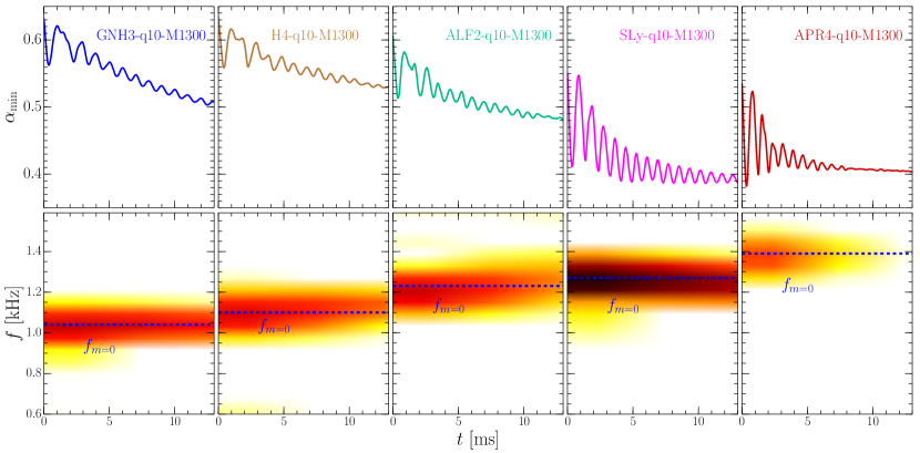
Figure 10: Evolution of the minimum of the lapse function after the merger (top panels) and the corresponding spectrograms (bottom panels), for all the cold EOSs and binaries with mass $\bar{M}=1.300M_{\odot}$. The horizontal blue dashed lines in the spectrograms indicate the fundamental quasi-radial oscillation frequencies $f_{m=0}$.

Appendix C Two-dimensional fit of $f_{\rm spiral}$

As mentioned in Sect. III.1, the frequency corresponding to $f_{\rm spiral}$ cannot be measured reliably in our simulations without the contamination of gauge effects. Hence, the values for these frequencies can be only obtained from the analytic expression provided in Ref. Bauswein and Stergioulas (2015), which refers uniquely to binaries with $\bar{M}=1.350\,M_{\odot}$ [cf., Eq. (2) of Bauswein and Stergioulas (2015)]. However, it is not difficult to perform a two-dimensional fit of the data presented in Fig. 7 of Bauswein and Stergioulas (2015) and obtain a fitting expression which is given by our Eq. (27) and can therefore be employed in principle for any interpolating mass (we recall that the data in Bauswein and Stergioulas (2015) refers to three sequences of binaries with $\bar{M}=1.200,1.350,1.500\,M_{\odot}$).

The goodness of our two-dimensional fit is shown in Fig. 11, where symbols of the different colour refer to the data presented in Fig. 7 of Ref. Bauswein and Stergioulas (2015) and thus to to the three sequences of binaries with mass $\bar{M}=1.200,1.350,1.500\,M_{\odot}$, respectively. Shown instead with the three solid lines is our fit for the three sequences, while the blue dashed line is the one given by Eq. (2) of Bauswein and Stergioulas (2015). Clearly, the two-dimensional fit (27) provides a very good representation of the data and has therefore been used to estimate the values of $f_{\rm spiral}$ in the various figures of this paper.

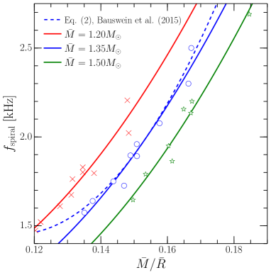
Figure 11: Two-dimensional fit of the data presented in Fig. 7 of Ref. Bauswein and Stergioulas (2015) referring to the three sequences of binaries with $\bar{M}=1.200,1.350,1.500\,M_{\odot}$, and shown with symbols of the different colour. The three solid lines represent our two-dimensional quadratic fit (27) for the three sequences, while the blue dashed line is the one given by Eq. (2) of Bauswein and Stergioulas (2015).

model	$f_{\rm max}$	$f_{1}$	$f_{2,i}$	$f_{2}$	$f_{m=0}$
	$[\mathrm{kHz}]$	$[\mathrm{kHz}]$	$[\mathrm{kHz}]$	$[\mathrm{kHz}]$	$[\mathrm{kHz}]$
GNH3-q10-M1200	$1.444$	$1.45$	$2.19$	$2.15$	$1.12$
GNH3-q10-M1225	$1.439$	$1.57$	$2.24$	$2.28$	$1.09$
GNH3-q10-M1250	$1.439$	$1.60$	$2.24$	$2.30$	$1.06$
GNH3-q10-M1275	$1.510$	$1.65$	$2.36$	$2.33$	$1.04$
GNH3-q10-M1300	$1.515$	$1.65$	$2.36$	$2.46$	$1.03$
GNH3-q10-M1325	$1.539$	$1.68$	$2.38$	$2.46$	$1.00$
GNH3-q10-M1350	$1.560$	$1.70$	$2.45$	$2.52$	$0.97$
GNH3-q10-M1375	$1.552$	$1.80$	$2.48$	$2.72$	$0.86$
GNH3-q10-M1400	$1.570$	$1.90$	$2.50$	$2.78$	$0.80$
GNH3-q10-M1500	$1.589$	$--$	$--$	$--$	$--$
GNH3-q09-M1300	$1.420$	$1.50$	$2.38$	$2.38$	$1.05$
GNH3-q08-M1275	$1.268$	$1.20$	$2.23$	$2.23$	$1.09$
ALF2-q10-M1200	$1.601$	$1.73$	$2.52$	$2.41$	$1.33$
ALF2-q10-M1225	$1.678$	$1.81$	$2.48$	$2.43$	$1.32$
ALF2-q10-M1250	$1.664$	$1.82$	$2.48$	$2.42$	$1.30$
ALF2-q10-M1275	$1.617$	$1.86$	$2.70$	$2.54$	$1.23$
ALF2-q10-M1300	$1.658$	$1.88$	$2.71$	$2.61$	$1.18$
ALF2-q10-M1325	$1.692$	$1.95$	$2.70$	$2.64$	$1.18$
ALF2-q10-M1350	$1.667$	$1.99$	$2.73$	$2.75$	$1.15$
ALF2-q10-M1375	$1.690$	$2.00$	$2.89$	$2.85$	$1.02$
ALF2-q10-M1400	$1.702$	$2.02$	$2.90$	$2.91$	$0.93$
ALF2-q10-M1500	$1.779$	$--$	$--$	$--$	$--$
H4-q10-M1200	$1.441$	$1.50$	$2.25$	$2.15$	$1.15$
H4-q10-M1225	$1.453$	$1.60$	$2.26$	$2.18$	$1.14$
H4-q10-M1250	$1.473$	$1.60$	$2.29$	$2.22$	$1.12$
H4-q10-M1275	$1.464$	$1.64$	$2.37$	$2.37$	$1.10$
H4-q10-M1300	$1.489$	$1.70$	$2.38$	$2.37$	$1.09$
H4-q10-M1325	$1.494$	$1.70$	$2.42$	$2.47$	$1.06$
H4-q10-M1350	$1.529$	$1.75$	$2.45$	$2.49$	$1.04$
H4-q10-M1375	$1.525$	$1.85$	$2.51$	$2.54$	$1.00$
H4-q10-M1400	$1.537$	$1.89$	$2.53$	$2.58$	$0.94$
H4-q10-M1500	$1.616$	$--$	$--$	$--$	$--$
SLy-q10-M1200	$1.948$	$1.84$	$3.11$	$3.00$	$1.36$
SLy-q10-M1225	$1.918$	$1.90$	$3.15$	$3.04$	$1.36$
SLy-q10-M1250	$1.947$	$2.00$	$3.23$	$3.00$	$1.31$
SLy-q10-M1275	$1.971$	$2.05$	$3.29$	$3.13$	$1.27$
SLy-q10-M1300	$1.954$	$2.13$	$3.34$	$3.22$	$1.26$
SLy-q10-M1325	$1.946$	$2.25$	$3.35$	$3.22$	$1.17$
SLy-q10-M1350	$1.991$	$2.37$	$3.37$	$3.29$	$1.11$
SLy-q10-M1375	$1.985$	$2.65$	$3.60$	$3.58$	$--$
SLy-q10-M1400	$2.002$	$--$	$3.35$	$3.31$	$--$
SLy-q10-M1500	$2.160$	$--$	$--$	$--$	$--$
SLy-q09-M1300	$1.940$	$2.20$	$3.30$	$3.11$	$1.29$
SLy-q08-M1275	$1.783$	$1.90$	$2.95$	$2.84$	$1.35$
APR4-q10-M1200	$1.959$	$1.90$	$3.21$	$3.02$	$1.43$
APR4-q10-M1225	$1.982$	$1.95$	$3.25$	$2.95$	$1.43$
APR4-q10-M1250	$1.992$	$2.00$	$3.30$	$3.04$	$1.40$
APR4-q10-M1275	$2.001$	$2.10$	$3.32$	$3.01$	$1.39$
APR4-q10-M1300	$2.035$	$2.17$	$3.36$	$3.14$	$1.36$
APR4-q10-M1325	$2.071$	$2.41$	$3.56$	$3.20$	$1.34$
APR4-q10-M1350	$2.056$	$2.52$	$3.60$	$3.25$	$1.31$
APR4-q10-M1375	$2.096$	$2.70$	$3.25$	$3.22$	$1.26$
APR4-q10-M1400	$2.109$	$2.85$	$3.37$	$3.28$	$1.19$
APR4-q10-M1500	$2.204$	$--$	$--$	$--$	$--$
LS220-q10-M1338	$1.703$	$1.92$	$2.95$	$2.93$	$1.06$
LS220-q10-M1372	$1.699$	$2.05$	$2.95$	$3.09$	$0.88$

Table 2: Values of the main spectral frequencies of the GW signals computed here: $f_{\rm max},f_{1}$, $f_{2,i}$, $f_{2}$ and $f_{m=0}$. In the case of high-mass binaries the post-merger phase is too short to obtain reliable measures of the peak frequencies, which are therefore not reported.

References

- Harry et al. (2010) G. M. Harry et al., Class. Quantum Grav. 27, 084006 (2010).
- Abbott et al. (2016) B. P. Abbott, R. Abbott, T. D. Abbott, M. R. Abernathy, F. Acernese, K. Ackley, C. Adams, T. Adams, P. Addesso, R. X. Adhikari, and et al., Phys. Rev. Lett. 116, 061102 (2016).
- Accadia et al. (2011) T. Accadia et al., Class. Quantum Grav. 28, 114002 (2011).
- Aso et al. (2013) Y. Aso, Y. Michimura, K. Somiya, M. Ando, O. Miyakawa, T. Sekiguchi, D. Tatsumi, and H. Yamamoto, Phys. Rev. D 88, 043007 (2013).
- Narayan et al. (1992) R. Narayan, B. Paczynski, and T. Piran, Astrophysical Journal, Letters 395, L83 (1992).
- Eichler et al. (1989) D. Eichler, M. Livio, T. Piran, and D. N. Schramm, Nature 340, 126 (1989).
- Berger (2014) E. Berger, Annual Review of Astron. and Astrophys. 52, 43 (2014).
- Shibata and Uryū (2000) M. Shibata and K. Uryū, Phys. Rev. D 61, 064001 (2000).
- Baiotti et al. (2008) L. Baiotti, B. Giacomazzo, and L. Rezzolla, Phys. Rev. D 78, 084033 (2008).
- Anderson et al. (2008a) M. Anderson, E. W. Hirschmann, L. Lehner, S. L. Liebling, P. M. Motl, D. Neilsen, C. Palenzuela, and J. E. Tohline, Phys. Rev. D 77, 024006 (2008a).
- Liu et al. (2008) Y. T. Liu, S. L. Shapiro, Z. B. Etienne, and K. Taniguchi, Phys. Rev. D 78, 024012 (2008).
- Bernuzzi et al. (2012a) S. Bernuzzi, M. Thierfelder, and B. Brügmann, Phys. Rev. D 85, 104030 (2012a).
- Ravi and Lasky (2014) V. Ravi and P. D. Lasky, Mon. Not. R. Astron. Soc. 441, 2433 (2014).
- Zhang and Mészáros (2001) B. Zhang and P. Mészáros, Astrophys. J. 552, L35 (2001).
- Metzger et al. (2011) B. D. Metzger, D. Giannios, T. A. Thompson, N. Bucciantini, and E. Quataert, Mon. Not. R. Astron. Soc. 413, 2031 (2011).
- Rezzolla and Kumar (2015) L. Rezzolla and P. Kumar, Astrophys. J. 802, 95 (2015).
- Ciolfi and Siegel (2015) R. Ciolfi and D. M. Siegel, Astrophys. J. 798, L36 (2015).
- Palenzuela et al. (2013) C. Palenzuela, L. Lehner, M. Ponce, S. L. Liebling, M. Anderson, D. Neilsen, and P. Motl, Phys. Rev. Lett. 111, 061105 (2013).
- Siegel et al. (2013) D. M. Siegel, R. Ciolfi, A. I. Harte, and L. Rezzolla, Phys. Rev. D R 87, 121302 (2013).
- Kiuchi et al. (2015) K. Kiuchi, P. Cerdá-Durán, K. Kyutoku, Y. Sekiguchi, and M. Shibata, Phys. Rev. D 92, 124034 (2015).
- Rezzolla et al. (2011) L. Rezzolla, B. Giacomazzo, L. Baiotti, J. Granot, C. Kouveliotou, and M. A. Aloy, Astrophys. J. Letters 732, L6 (2011).
- Paschalidis et al. (2015) V. Paschalidis, M. Ruiz, and S. L. Shapiro, Astrophys. J. Lett. 806, L14 (2015).
- Flanagan and Hinderer (2008) É. É. Flanagan and T. Hinderer, Phys. Rev. D 77, 021502 (2008).
- Baiotti et al. (2010) L. Baiotti, T. Damour, B. Giacomazzo, A. Nagar, and L. Rezzolla, Phys. Rev. Lett. 105, 261101 (2010).
- Bernuzzi et al. (2012b) S. Bernuzzi, A. Nagar, M. Thierfelder, and B. Brügmann, Phys. Rev. D 86, 044030 (2012b).
- Bernuzzi et al. (2015a) S. Bernuzzi, A. Nagar, T. Dietrich, and T. Damour, Phys. Rev. Lett. 114, 161103 (2015a).
- Hinderer et al. (2016) T. Hinderer, A. Taracchini, F. Foucart, A. Buonanno, J. Steinhoff, M. Duez, L. E. Kidder, H. P. Pfeiffer, M. A. Scheel, B. Szilagyi, K. Hotokezaka, K. Kyutoku, M. Shibata, and C. W. Carpenter, arXiv:1602.00599 (2016).
- Radice et al. (2014a) D. Radice, L. Rezzolla, and F. Galeazzi, Mon. Not. R. Astron. Soc. L. 437, L46 (2014a).
- Radice et al. (2014b) D. Radice, L. Rezzolla, and F. Galeazzi, Class. Quantum Grav. 31, 075012 (2014b).
- Radice et al. (2015) D. Radice, L. Rezzolla, and F. Galeazzi, Numerical Modeling of Space Plasma Flows ASTRONUM-2014, Astronomical Society of the Pacific Conference Series, 498, 121 (2015).
- Hotokezaka et al. (2016) K. Hotokezaka, K. Kyutoku, Y.-i. Sekiguchi, and M. Shibata, arXiv:1603.01286 (2016).
- Read et al. (2013) J. S. Read, L. Baiotti, J. D. E. Creighton, J. L. Friedman, B. Giacomazzo, K. Kyutoku, C. Markakis, L. Rezzolla, M. Shibata, and K. Taniguchi, Phys. Rev. D 88, 044042 (2013).
- Bernuzzi et al. (2014a) S. Bernuzzi, A. Nagar, S. Balmelli, T. Dietrich, and M. Ujevic, Phys. Rev. Lett. 112, 201101 (2014a).
- Takami et al. (2015) K. Takami, L. Rezzolla, and L. Baiotti, Phys. Rev. D 91, 064001 (2015).
- Shibata (2005) M. Shibata, Phys. Rev. Lett. 94, 201101 (2005).
- Oechslin and Janka (2007) R. Oechslin and H.-T. Janka, Phys. Rev. Lett. 99, 121102 (2007).
- Bauswein and Janka (2012) A. Bauswein and H.-T. Janka, Phys. Rev. Lett. 108, 011101 (2012).
- Stergioulas et al. (2011) N. Stergioulas, A. Bauswein, K. Zagkouris, and H.-T. Janka, Mon. Not. R. Astron. Soc. 418, 427 (2011).
- Bauswein et al. (2012) A. Bauswein, H.-T. Janka, K. Hebeler, and A. Schwenk, Phys. Rev. D 86, 063001 (2012).
- Hotokezaka et al. (2013) K. Hotokezaka, K. Kiuchi, K. Kyutoku, T. Muranushi, Y.-i. Sekiguchi, M. Shibata, and K. Taniguchi, Phys. Rev. D 88, 044026 (2013).
- Bauswein et al. (2014) A. Bauswein, N. Stergioulas, and H.-T. Janka, Phys. Rev. D 90, 023002 (2014).
- Takami et al. (2014) K. Takami, L. Rezzolla, and L. Baiotti, Phys. Rev. Lett. 113, 091104 (2014).
- Bernuzzi et al. (2015b) S. Bernuzzi, T. Dietrich, and A. Nagar, Phys. Rev. Lett. 115, 091101 (2015b).
- Palenzuela et al. (2015) C. Palenzuela, S. L. Liebling, D. Neilsen, L. Lehner, O. L. Caballero, E. O’Connor, and M. Anderson, Phys. Rev. D 92, 044045 (2015).
- Bauswein and Stergioulas (2015) A. Bauswein and N. Stergioulas, Phys. Rev. D 91, 124056 (2015).
- Dietrich et al. (2015) T. Dietrich, S. Bernuzzi, M. Ujevic, and B. Brügmann, Phys. Rev. D 91, 124041 (2015).
- Foucart et al. (2016) F. Foucart, R. Haas, M. D. Duez, E. O’Connor, C. D. Ott, L. Roberts, L. E. Kidder, J. Lippuner, H. P. Pfeiffer, and M. A. Scheel, Phys. Rev. D 93, 044019 (2016).
- Lehner et al. (2016) L. Lehner, S. L. Liebling, C. Palenzuela, O. L. Caballero, E. O’Connor, M. Anderson, and D. Neilsen, arXiv:1603.00501 (2016).
- Baiotti et al. (2009) L. Baiotti, B. Giacomazzo, and L. Rezzolla, Class. Quantum Grav. 26, 114005 (2009).
- Baiotti et al. (2010) L. Baiotti, M. Shibata, and T. Yamamoto, Phys. Rev. D 82, 064015 (2010).
- Brown et al. (2009) D. Brown, P. Diener, O. Sarbach, E. Schnetter, and M. Tiglio, Phys. Rev. D 79, 044023 (2009).
- Löffler et al. (2012) F. Löffler, J. Faber, E. Bentivegna, T. Bode, P. Diener, R. Haas, I. Hinder, B. C. Mundim, C. D. Ott, E. Schnetter, G. Allen, M. Campanelli, and P. Laguna, Class. Quantum Grav. 29, 115001 (2012).
- Nakamura et al. (1987) T. Nakamura, K. Oohara, and Y. Kojima, Progress of Theoretical Physics Supplement 90, 1 (1987).
- Shibata and Nakamura (1995) M. Shibata and T. Nakamura, Phys. Rev. D 52, 5428 (1995).
- Baumgarte and Shapiro (1999) T. W. Baumgarte and S. L. Shapiro, Phys. Rev. D 59, 024007 (1999).
- Alcubierre et al. (2003) M. Alcubierre, B. Brügmann, P. Diener, M. Koppitz, D. Pollney, E. Seidel, and R. Takahashi, Phys. Rev. D 67, 084023 (2003).
- Pollney et al. (2007) D. Pollney, C. Reisswig, L. Rezzolla, B. Szilágyi, M. Ansorg, B. Deris, P. Diener, E. N. Dorband, M. Koppitz, A. Nagar, and E. Schnetter, Phys. Rev. D 76, 124002 (2007).
- Baiotti et al. (2005) L. Baiotti, I. Hawke, P. J. Montero, F. Löffler, L. Rezzolla, N. Stergioulas, J. A. Font, and E. Seidel, Phys. Rev. D 71, 024035 (2005).
- Rezzolla et al. (2010) L. Rezzolla, L. Baiotti, B. Giacomazzo, D. Link, and J. A. Font, Class. Quantum Grav. 27, 114105 (2010).
- Harten et al. (1983) A. Harten, P. D. Lax, and B. van Leer, SIAM Rev. 25, 35 (1983).
- Colella and Woodward (1984) P. Colella and P. R. Woodward, Journal of Computational Physics 54, 174 (1984).
- Rezzolla and Zanotti (2013) L. Rezzolla and O. Zanotti, Relativistic Hydrodynamics (Oxford University Press, Oxford, UK, 2013).
- Kastaun et al. (2013) W. Kastaun, F. Galeazzi, D. Alic, L. Rezzolla, and J. A. Font, Phys. Rev. D 88, 021501 (2013).
- Schnetter et al. (2004) E. Schnetter, S. H. Hawley, and I. Hawke, Class. Quantum Grav. 21, 1465 (2004).
- Akmal et al. (1998) A. Akmal, V. R. Pandharipande, and D. G. Ravenhall, Phys. Rev. C 58, 1804 (1998).
- Alford et al. (2005) M. Alford, M. Braby, M. Paris, and S. Reddy, Astrophys. J. 629, 969 (2005).
- Douchin and Haensel (2001) F. Douchin and P. Haensel, Astron. Astrophys. 380, 151 (2001).
- Glendenning and Moszkowski (1991) N. K. Glendenning and S. A. Moszkowski, Phys. Rev. Lett. 67, 2414 (1991).
- Glendenning (1985) N. K. Glendenning, Astrophys. J. 293, 470 (1985).
- Antoniadis et al. (2013) J. Antoniadis, P. C. C. Freire, N. Wex, T. M. Tauris, R. S. Lynch, M. H. van Kerkwijk, M. Kramer, C. Bassa, V. S. Dhillon, T. Driebe, J. W. T. Hessels, V. M. Kaspi, V. I. Kondratiev, N. Langer, T. R. Marsh, M. A. McLaughlin, T. T. Pennucci, S. M. Ransom, I. H. Stairs, J. van Leeuwen, J. P. W. Verbiest, and D. G. Whelan, Science 340, 448 (2013).
- Lattimer and Swesty (1991) J. M. Lattimer and F. D. Swesty, Nucl. Phys. A 535, 331 (1991).
- Radice et al. (2016) D. Radice, F. Galeazzi, J. Lippuner, L. F. Roberts, C. D. Ott, and L. Rezzolla, ArXiv e-prints (2016).
- Read et al. (2009) J. S. Read, B. D. Lackey, B. J. Owen, and J. L. Friedman, Phys. Rev. D 79, 124032 (2009).
- Janka et al. (1993) H.-T. Janka, T. Zwerger, and R. Mönchmeyer, Astron. Astrophys. 268, 360 (1993).
- Gourgoulhon et al. (2001) E. Gourgoulhon, P. Grandclément, K. Taniguchi, J.-A. Marck, and S. Bonazzola, Phys. Rev. D 63, 064029 (2001).
- Goldberg et al. (1967) J. N. Goldberg, A. J. MacFarlane, E. T. Newman, F. Rohrlich, and E. C. G. Sudarshan, J. Math. Phys. 8, 2155 (1967).
- (77) Advanced LIGO anticipated sensitivity curves, LIGO Document No. T0900288-v3.
- Punturo et al. (2010a) M. Punturo et al., Class. Quantum Grav. 27, 084007 (2010a).
- Punturo et al. (2010b) M. Punturo et al., Class. Quantum Grav. 27, 194002 (2010b).
- Bauswein et al. (2016) A. Bauswein, N. Stergioulas, and H.-T. Janka, European Physical Journal A 52, 56 (2016).
- Font et al. (2000) J. A. Font, N. Stergioulas, and K. D. Kokkotas, Mon. Not. R. Astron. Soc. 313, 678 (2000).
- Font et al. (2002) J. A. Font, T. Goodale, S. Iyer, M. Miller, L. Rezzolla, E. Seidel, N. Stergioulas, W.-M. Suen, and M. Tobias, Phys. Rev. D 65, 084024 (2002).
- Radice and Rezzolla (2011) D. Radice and L. Rezzolla, Phys. Rev. D 84, 024010 (2011).
- Tsatsin and Marronetti (2013) P. Tsatsin and P. Marronetti, Phys. Rev. D 88, 064060 (2013).
- Bernuzzi et al. (2014b) S. Bernuzzi, T. Dietrich, W. Tichy, and B. Brügmann, Phys. Rev. D 89, 104021 (2014b).
- Tsokaros et al. (2015) A. Tsokaros, K. Uryū, and L. Rezzolla, Phys. Rev. D 91, 104030 (2015).
- Kastaun and Galeazzi (2015) W. Kastaun and F. Galeazzi, Phys. Rev. D 91, 064027 (2015).
- Giacomazzo et al. (2011) B. Giacomazzo, L. Rezzolla, and L. Baiotti, Phys. Rev. D 83, 044014 (2011).
- Dionysopoulou et al. (2015) K. Dionysopoulou, D. Alic, and L. Rezzolla, Phys. Rev. D 92, 084064 (2015).
- Ou and Tohline (2006) S. Ou and J. E. Tohline, Astrophys. J. 651, 1068 (2006).
- Corvino et al. (2010) G. Corvino, L. Rezzolla, S. Bernuzzi, R. De Pietri, and B. Giacomazzo, Class. Quantum Grav. 27, 114104 (2010).
- Anderson et al. (2008b) M. Anderson, E. W. Hirschmann, L. Lehner, S. L. Liebling, P. M. Motl, D. Neilsen, C. Palenzuela, and J. E. Tohline, Phys. Rev. Lett. 100, 191101 (2008b).
- East et al. (2016) W. E. East, V. Paschalidis, F. Pretorius, and S. L. Shapiro, Phys. Rev. D 93, 024011 (2016).
- Breu and Rezzolla (2016) C. Breu and L. Rezzolla, Mon. Not. R. Astron. Soc. 459, 646 (2016).
- Damour et al. (2012) T. Damour, A. Nagar, and L. Villain, Phys. Rev. D 85, 123007 (2012).