Accurate numerical simulations of inspiralling binary neutron stars
and their comparison with effective-one-body analytical models
Abstract
Binary neutron-star systems represent one of the most promising sources of gravitational waves. In order to be able to extract important information, notably about the equation of state of matter at nuclear density, it is necessary to have in hands an accurate analytical model of the expected waveforms. Following our recent work Baiotti et al. (2010), we here analyze more in detail two general-relativistic simulations spanning about gravitational-wave cycles of the inspiral of equal-mass binary neutron stars with different compactnesses, and compare them with a tidal extension of the effective-one-body (EOB) analytical model. The latter tidally extended EOB model is analytically complete up to the 1.5 post-Newtonian level, and contains an analytically undetermined parameter representing a higher-order amplification of tidal effects. We find that, by calibrating this single parameter, the EOB model can reproduce, within the numerical error, the two numerical waveforms essentially up to the merger. By contrast, analytical models (either EOB or Taylor-T4) that do not incorporate such a higher-order amplification of tidal effects, build a dephasing with respect to the numerical waveforms of several radians.
pacs:
04.25.dk, 04.25.Nx, 04.30.Db, 04.40.Dg, 95.30.Sf, 97.60.JdI Introduction
Binary neutron-star inspirals are among the most promising and certain target sources for the advanced versions of the currently operating ground-based gravitational-wave (GW) detectors LIGO/Virgo/GEO. These detectors will be maximally sensitive during the inspiral part of the signal (around a GW frequency of Hz, i.e., significantly below the typical GW frequencies at merger, which are around Hz). The inspiral part of the signal will be influenced by tidal interaction between the two neutron stars (NSs), which, in turn, encodes important information about the equation of state (EOS) of matter at nuclear densities. In other words, the detection of GWs emitted from inspiralling NS in the LIGO/Virgo bandwidth could enable us to acquire important information about the EOS of NS matter. However, besides getting sufficiently accurate GW data from advanced detectors, two conditions must be fulfilled for the success of this program: (i) obtaining a large enough sample of accurate numerical simulations of inspiralling binary neutron stars (BNS); (ii) possessing a sufficiently accurate analytical model of inspiralling BNS, allowing the extrapolation of the finite set of numerical simulations to the multi-parameter space of possible GW templates. Extending the work recently reported in Baiotti et al. (2010), we here address issues and provide useful progress on both of them. In essence, we will present the results of general-relativistic simulations spanning about gravitational-wave cycles of the inspiral of equal-mass BNSs, and show how a suitably calibrated effective-one-body (EOB) analytical model of tidally interacting BNS systems enables us to accurately reproduce the numerically simulated inspiral waveform.
Numerical simulations of merging BNSs in full general relativity have a long history (see the Introduction of Baiotti et al. (2008) for a brief review), and the first merger to a hypermassive neutron star (HMNS) was computed more than ten years ago Shibata and Uryū (2000). However, it is only in recent years and with the use of more advanced and accurate numerical algorithms that it has been possible to obtain a more precise and robust description of this process and to include additional physical ingredients such as magnetic fields and realistic EOSs. In particular the use of adaptive mesh refinement techniques Anderson et al. (2008); Baiotti et al. (2008); Yamamoto et al. (2008) made it possible to use very high resolutions, increasing not only the level of accuracy, but giving the possibility, for example, to compute the full evolution of the HMNS up to black-hole (BH) formation Baiotti et al. (2008) or to investigate in detail the development of hydrodynamical instabilities at the time of the merger Baiotti et al. (2008). Also the numerical convergence properties of BNS simulations have been studied only recently Baiotti et al. (2009a), providing for the first time evidence of the level of accuracy that it is now possible to achieve in the generation of GW templates from these sources. Several groups are now able to simulate BNSs using more realistic EOSs (see, e.g., Read et al. (2009); Kiuchi et al. (2009, 2010) and references therein) and to assess the possibility to measure their effects in the GW signals. In the last two years three different groups were also able to perform for the first time the simulations of magnetized BNSs Anderson et al. (2008); Liu et al. (2008); Giacomazzo et al. (2009). One conclusion already reached is that no effect of the magnetic field can be measured in the inspiral waveforms Giacomazzo et al. (2009), while the role of the magnetic field in the post-merger phase has been recently investigated in Giacomazzo et al. (2011) as well as its role in the emission of relativistic jets after the collapse to BH Rezzolla et al. (2011). Because of their possible connection with the production of short gamma-ray bursts (GRBs), numerical simulations have also investigated in detail the formation of massive tori and their dependence on the initial mass and mass ratio of the binary (see e.g., Rezzolla et al. (2010)) as well as on the EOS used (see Kiuchi et al. (2009, 2010) and references therein).
On the other hand, the program of developing an analytical description within general relativity of tidally-interacting binary systems has been initiated only recently Flanagan and Hinderer (2008); Hinderer (2008); Damour and Nagar (2009); Binnington and Poisson (2009); Hinderer et al. (2010); Damour and Nagar (2010); Pannarale et al. (2011). Overall, this work has brought to light two surprising results. First, that the dimensionless expression (Love number) in the (gravito-electric) tidal polarizability parameter measuring the relativistic coupling (of multipolar order ) between a NS of radius and the external gravitational field in which it is embedded strongly decreases with the compactness parameter of the NS Damour and Nagar (2009); Binnington and Poisson (2009)111As a consequence, for a given EOS, the Love numbers of a typical () NS are found to be about time smaller than their corresponding Newtonian estimates, that assume .. Second, a recent comparison between a numerical computation of the binding energy of quasi-equilibrium circular sequences of BNS systems Uryu et al. (2009) and the EOB description of tidal effects Damour and Nagar (2010) suggests that high-order (beyond the first order) post-Newtonian (PN) corrections to tidal effects tend to significantly increase (typically by a factor of order two) the effective tidal polarizability of NSs.
The main aim of this paper is to present a detailed comparison between waveforms computed from the tidal-completed EOB analytical model of Ref. Damour and Nagar (2010) and waveforms from BNS simulations comprising between and GW cycles of inspiral Baiotti et al. (2010). More specifically, we will follow Ref. Damour and Nagar (2010), which has proposed a new way of analytically describing the dynamics of tidally interacting BNSs, whose validity is not a priori limited (like the purely PN-based descriptions used in, e.g., Flanagan and Hinderer (2008)) to the low-frequency part of the GW signal, but may be extended to higher frequencies, essentially up to the merger. The proposal of Ref. Damour and Nagar (2010) consists in extending the EOB method Buonanno and Damour (1999, 2000); Damour (2001), which has recently shown its ability to accurately describe the GW waveforms emitted by inspiralling, merging, and ringing binary black holes (BBHs) Damour and Nagar (2009a); Buonanno et al. (2009), by incorporating tidal effects in it. We will improve the tidally-extended EOB model of Ref. Damour and Nagar (2010) (which already contained the 1PN contributions to the dynamics) by incorporating the 1PN contributions to the waveform (from Vines et al. (2011)), as well as the waveform tail effects (from Blanchet and Damour (1992); Damour and Nagar (2008)).
The paper is organized as follows. In Sec. II we present in detail our numerical simulations, briefly reviewing our numerical setup, discussing the dynamics of the binaries, and presenting the main features of the waveforms. Section III deals instead with the analytical models of the binary dynamics and of waveforms that include tidal interaction (either PN-based or EOB-based). Sec. IV introduces some tools, notably a certain intrinsic representation of the time evolution of the GW frequency, which is useful for doing the numerical-relativity/analytical-relativity (NR/AR) comparison. Section V discusses the various errors that affect the NR phasing. The NR/AR comparison is carried out in Sec. VI. We finally present a summary of our findings in Sec. VII. Two appendices give additional technical details on the use of the waveforms from the numerical-relativity simulations.
We use a spacelike signature and (unless explicitly said otherwise) a system of units in which . Greek indices are taken to run from to , Latin indices from to .
II Numerical-relativity simulations
II.1 Numerical setup
The numerical simulations were performed with the set of codes Cactus-Carpet-Whisky Goodale et al. (2003); Schnetter et al. (2004); Pollney et al. (2007); Baiotti et al. (2003, 2005). The reader is referred to these references for the description of the details of the implementations and of the tests of the codes. Since in this work we use the same gauges and numerical methods already applied and explained in Baiotti et al. (2008, 2009a), we also refer the reader to these articles for more detailed explanations of the setup only briefly recalled below.
| Model | |||||||||||
|---|---|---|---|---|---|---|---|---|---|---|---|
| () | () | () | () | () | () | () | |||||
| M2.9C.12 | |||||||||||
| M3.2C.14 |
In essence, we evolve a conformal-traceless “” formulation of the Einstein equations in which the spacetime is decomposed into three-dimensional spacelike slices, described by a metric , its embedding in the full spacetime, specified by the extrinsic curvature , and the gauge functions (lapse) and (shift), which specify a coordinate frame (see Ref. Pollney et al. (2007) for details on the latest implementation of the Einstein equations in the code). For the evolution of the matter, the Whisky code implements the flux-conservative formulation of the general-relativistic hydrodynamics equations proposed by the Valencia group Banyuls et al. (1997). Among its important features is that the set of conservation equations for the stress-energy tensor and for the matter current density are written in hyperbolic, first-order, and flux-conservative form (see Ref. Baiotti et al. (2008) for details on the latest implementation of the hydrodynamics equations in the code).
As initial data we use quasi-equilibrium binaries generated with the multi-domain spectral-method code LORENE developed at the Observatoire de Paris-Meudon Gourgoulhon et al. (2001). For more information on the code and its methods, the reader is referred to the LORENE web pages Lor . In particular, we use irrotational configurations, defined as having vanishing vorticity and obtained under the additional assumption of a conformally flat spacetime metric Gourgoulhon et al. (2001). The EOS assumed for the initial data is in all cases the polytropic EOS
| (1) |
where and are the pressure and the rest-mass (baryonic-mass) density, respectively. The chosen adiabatic index is , while the polytropic constant is (in units where ). For this particular EOS, the allowed maximum baryonic mass for an individual stable NS is , thus leading to a maximum compactness . The initial coordinate separation of the stellar centers in all cases is .
The physical properties of the two binaries considered here are summarized in Table 1, where we have adopted the following naming convention: M%C#, with % being replaced by the rounded total baryonic mass of the binary NS system and # by the compactness. As an example, M2.9C.12 is the binary with total baryonic mass and compactness . We note that at least as far as the tidal effects are concerned, the most important difference in the two sets of initial data is represented by the compactness, which is smaller in the binary M2.9C.12 than in the binary M3.2C.14. Note that the dimensionless EOB parameter measuring the strength of the (conservative) quadrupolar interaction is nearly three times larger for , than for .
The initial data is then evolved either using the (isentropic) polytropic EOS (1) or using the (non-isentropic) “ideal-fluid” EOS defined by the condition
| (2) |
where is the specific internal energy and is the total energy density. Although these EOSs are idealized, they provide a reasonable approximation of the dynamics of NSs during the inspiral, so that we expect that the use of realistic EOSs (with similar compactnesses) would not change the main qualitative conclusions of this work. A detailed discussion of the consequences of using either EOS will be presented in Sec. V.
As mentioned above, the use of adaptive mesh-refinement techniques allows us to reach a considerable level of precision and for this we use the Carpet code Schnetter et al. (2004) that implements a vertex-centered adaptive-mesh-refinement scheme adopting nested grids with a refinement factor for successive grid levels. We center the highest resolution level around the peak in the rest-mass density of each star. This represents our rather basic form of adaptive-mesh refinement. The timestep on each grid is set by the Courant condition (expressed in terms of the speed of light) and so by the spatial grid resolution for that level; the typical Courant coefficient is set to be . The time evolution is carried out using fourth-order accurate Runge-Kutta integration steps. Boundary data for finer grids are calculated with spatial prolongation operators employing fifth-order polynomials and with prolongation in time employing second-order polynomials.
In the results presented below we have used levels of mesh refinement with the finest grid resolution of and the coarsest (or wave-zone) grid resolution of . Each star is completely covered by the finest grid, so that the high-density regions of the stars are tracked with the highest resolution available. The refined grids are then moved by tracking the position of the maximum of the rest-mass density as the stars orbit, and are finally merged when they overlap. In addition, a set of refined but fixed grids is set up at the center of the computational domain so as to capture the details of the Kelvin-Helmholtz instability (cf. Baiotti et al. (2008)). The finest of these grids extends to for model M2.9C.12 and for model M3.2C.14 (here and in the following denotes the gravitational mass of the system at infinite separation, namely the sum of the gravitational masses of each NS as computed individually in isolation, i.e., in the notation of Table 1). A single grid-resolution covers then the region between and (or for M2.9C.12 and for M3.2C.14), in which our wave extraction is carried out. The resolution is here and thus more than sufficient to accurately resolve the gravitational waveforms that have initially a wavelength of about .
A reflection symmetry condition across the plane and a -symmetry condition222Stated differently, we evolve only the region applying a 180-degree rotational-symmetry boundary condition across the plane at . across the plane are used. A number of tests have been performed to ensure that both the hierarchy of the refinement levels described above and the resolutions used yield results that are numerically consistent although not always in a convergent regime at the time of merger (see the detailed discussion in Ref. Baiotti et al. (2009a)).
II.2 Overall matter dynamics and gravitational waveforms
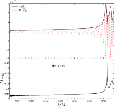
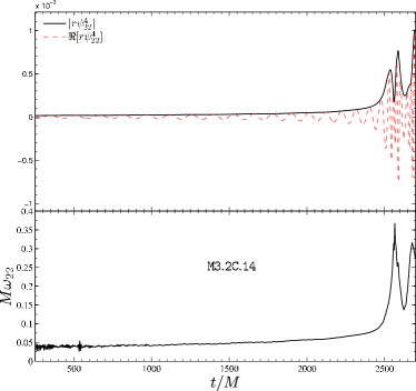
We next briefly recall the physical properties of BNS inspiral and merger as discussed in Refs. Baiotti et al. (2008, 2009a). The inspiral proceeds at higher and higher frequencies until the time of the merger, just before which the stars decompress because of the tidal force. At the time of the merger, a Kelvin-Helmholtz instability develops in the shearing layer formed by the colliding stars, which could lead to an exponential growth of magnetic fields if these are present Price and Rosswog (2006); Obergaulinger et al. (2010); such a large growth was not found in recent related works Giacomazzo et al. (2009, 2011), and no magnetic fields are included in the simulations reported here. If the total mass of the system is sufficiently large, the merged object immediately collapses to a Kerr BH, while, for smaller masses the merger remnant is a HMNS in a metastable equilibrium. Because of the excess angular momentum, the HMNS is also subject to a bar deformation, being responsible for a copious emission of gravitational radiation with peak amplitudes that are comparable or even larger than those at the merger (cf. Ref. Baiotti et al. (2008)). As the bar-deformed HMNS loses energy and angular momentum via GWs, it contracts and spins up, thus further increasing the losses. The process terminates when the threshold to the collapse to BH is crossed and the HMNS then rapidly produces a rotating BH surrounded by a torus of hot and high-density material. Although this post-merger evolution of the binary is of great interest and is likely to yield a wealth of physical information, it will not be further considered in the present work, which is instead focussed on the analytical modelling of the inspiral phase, up to the merger.
The GW signal is extracted at different surfaces of constant coordinate radius by means of two distinct methods. The first one is based on the measurements of the non-spherical gauge-invariant perturbations of a Schwarzschild BH Nagar and Rezzolla (2005, 2006). The second and independent one uses instead the Newman-Penrose formalism so that the GW (metric) polarization amplitudes and are then related to by (see Sec. IV of Ref. Baiotti et al. (2008) for details of the Newman-Penrose scalar extraction in our setup)
| (3) |
where we have introduced the (multipolar) expansion of in spin-weighted spherical harmonics Goldberg et al. (1967) of spin-weight . The coordinate extraction radius is for both models, which corresponds to for M2.9C.12 and to for M3.2C.14. The top panels of Fig. 1 summarizes most of the information related to the curvature waveforms for the M2.9C.12 model (left panels) and for the M3.2C.14 model (right panels). The top panels of the figures show together the modulus and the real part of the waveform; the bottom ones, illustrate the behavior of the instantaneous GW (curvature) frequency . Note that the inspiral waveform of M2.9C.12 contains about 22 GW cycles, while that of M3.2C.14 contains about GW cycles. To fix conventions, let us recall that we write the waveform as a complex number according to
| (4) |
so that the instantaneous (curvature) GW frequency is simply defined as . After the initial junk radiation (cf. Ref. Baiotti et al. (2009b)) that is responsible for a spike in the modulus around together with incoherent oscillations in the frequency, the complex waveform becomes circularly polarized (as expected for circularized inspiral), with a modulus that grows monotonically in time up to the merger (see upper panels of Fig. 1).
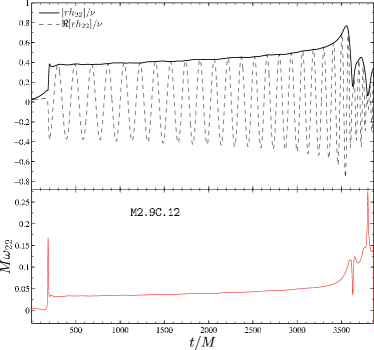
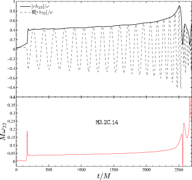
The matter dynamics is reflected in the behavior of the frequency: for both models we clearly see that grows monotonically during the inspiral phase, until it reaches a maximum around the “merger”. In this work, we phenomenologically define the “NR merger” as the instant when the modulus of the metric waveform (see below) reaches its (first) maximum. Roughly speaking, in our simulations the “dynamical range” of the dimensionless GW frequency parameter during the inspiral (i.e., before the merger) is . Note that, if we were considering a conventional BNS system, we would then have the correspondence so that corresponds to Hz, while corresponds to Hz.
In order to perform direct comparisons with (resummed) analytical waveforms and since the resummations used in the EOB method have been developed (and tested) mainly for metric waveforms, we derived the metric waveform by a (double) time-integration of the waveform (the so-obtained metric waveform was found to be more accurate than the output of the gauge-invariant perturbation scheme). We recall that the metric waveform is also expanded in spin-weighted spherical harmonics with the following convention
| (5) |
so that the metric multipoles at time can be obtained from by double time-integration as
| (6) |
This expression assumes that one knows the curvature waveform on the infinite time interval . Since, however, the simulated curvature waveform does not start at an infinite time in the past, but at a finite (conventional) time , one has to find a way of determining two (complex) integration constants accounting from the GW emission from infinite time to our present starting time. To do so, we use here an improved version of the fit procedure of Ref. Damour et al. (2008a), which is presented in detail in Appendix A. Figure 2 shows the result of this process, with the left panels referring to model M2.9C.12 and the right ones to model M3.2C.14. Note that the waveforms displayed in these figures are obtained from simulations with: (i) the non-isentropic (ideal fluid) EOS; (ii) the highest available resolution; and (iii) an extraction radius of . These will be taken as our fiducial “target” waveforms for our NR/AR comparisons, and we will refer to them in the following with the label . The numerical uncertainty on these target waveforms will be estimated in Sec. V below.
III Analytical models
We recall below some basic information relative to the EOB-based and PN-based descriptions of the binary dynamics and waveforms that include tidal effects. We follow here the general discussion of Ref. Damour and Nagar (2010), to which we refer the reader for more details. We consider successively: (i) the resummed EOB description of the conservative dynamics, (ii) the resummed EOB description of the waveform, and (iii) one of the non-resummed (i.e., PN expanded) descriptions of the phasing.
III.1 Effective-one-body description of the conservative dynamics
The EOB formalism Buonanno and Damour (1999, 2000); Damour (2001) replaces the PN-expanded two-body interaction Lagrangian (or Hamiltonian) by a resummed Hamiltonian, of a specific form, which depends only on the relative position and momentum of the binary system . For a non spinning BBH system, it has been shown that its dynamics, up to the 3PN level, can be described by the following EOB Hamiltonian (in polar coordinates, within the plane of the motion):
| (7) |
where
| (8) |
Here is the total mass, is the symmetric mass ratio, and . In addition, we are using rescaled dimensionless (effective) variables, namely and , and is canonically conjugated to a “tortoise” modification of Damour and Nagar (2009b).
A remarkable feature of the EOB formalism is that the complicated, original 3PN Hamiltonian (which contains many corrections to the basic Newtonian Hamiltonian ) can be replaced by the simple structure (7)-(8), whose two crucial ingredients are: (i) a “double square-root” structure and (ii) the “condensation” of most of the nonlinear relativistic gravitational interactions in one function of the (EOB) radial variable: the basic “radial potential” . The structure of the function is rather simple at 3PN, being given by
| (9) |
where , and . It was recently found that an excellent description of the dynamics of BBH systems is obtained Damour and Nagar (2009a) by: (i) augmenting the presently computed terms in the PN expansion (9) by additional 4PN and 5PN terms; (ii) Padé-resumming the corresponding 5PN “Taylor” expansion of the function. In other words, the BBH (or “point mass”) dynamics is well described by a function of the form
| (10) |
where denotes an Padé approximant. It was found in Ref. Damour and Nagar (2009a) that a good agreement between EOB and numerical-relativity BBH waveforms is obtained in an extended “banana-like” region in the plane approximately spanning the interval between the points and . In this work we will select the values , , which lie within this region (we have checked that the use of other values within the “good BBH fit” region would have no measurable influence on our discussion below).
The proposal of Ref. Damour and Nagar (2010) for including dynamical tidal effects in the conservative part of the dynamics consists in simply using Eqs. (7)-(8) with the following tidally-augmented radial potential
| (11) |
Here is the point-mass potential defined in Eq. (10), while is a supplementary “tidal contribution” of the form
| (12) |
where the terms represent the leading-order (LO) tidal interaction, i.e., the Newtonian order tidal interaction. The dynamical EOB tidal coefficients are functions of the two masses and , of the two compactnesses , and of the two (relativistic) Love numbers of the two objects Damour and Nagar (2009); Binnington and Poisson (2009); Hinderer et al. (2010):
| (13) | |||||
where the second line refers to an equal-mass binary, as the ones considered here. Note in Table I the rather large numerical values for the tidal coefficients: and . In our EOB modelling we also use the higher multipolar tidal coefficients and , which are even larger than (e.g., ), although their effect is marginal in view of the higher power of (namely ) with which they enter the potential.
The additional factor in Eq. (12) represents the effect of higher-order relativistic contributions to the dynamical tidal interactions: next-to-leading–order (NLO) contributions, next-to-next-to-leading–order (NNLO) contributions, etc. Here we will consider a “Taylor-expanded” expression
| (14) |
where are functions of , , and for a general binary. The analytical value of the () 1PN coefficient has been reported in Damour and Nagar (2010) (and recently confirmed in Vines et al. (2011)). In the equal-mass case, it yields . By contrast, there are no analytical calculations available for with , nor for the 2PN tidal coefficients . Indeed, one of the main aims of the present work will be to constrain the value of by comparing the EOB predictions to numerical data.
III.2 Effective-one-body description of the waveform and radiation reaction
Let us first recall that the EOB formalism defines the radiation reaction from the angular-momentum flux computed from the waveform. Concerning the waveform, in the case of BBH systems, the EOB formalism replaces the PN-expanded multipolar (metric) waveform by a specifically resummed “factorized waveform” Damour and Nagar (2008); Damour et al. (2009), say (where the superscript is added to signal the absence of tidal effects). This tidal-free multipolar waveform includes resummed versions of very high-order PN effects in the phase and the modulus, in particular tail effects. Actually, in the present work, we have used a factorized waveform which includes in the modulus (but not in the phase) the new (5PN accurate) terms recently computed in Fujita and Iyer (2010)333 As in Ref. Damour et al. (2009) we resum the modulus by using the Padé-resummed function .. We also included in the two next-to-quasi-circular parameters as in Ref. Damour and Nagar (2009a)444 Since both M2.9C.12 and M3.2C.14 are equal-mass binaries, we fix and , according to the EOB/NR comparison (for a BBH equal-mass system) of Ref. Damour and Nagar (2009a)..
When considering tidally interacting binary systems, one needs to augment the BBH waveform by tidal contributions. Similarly to the additive tidal modification (11) of the potential, we will here consider an additive modification of the waveform, having the structure
| (15) |
This is slightly different from the factorized form introduced in Eq. (71) of Damour and Nagar (2010) and used in Baiotti et al. (2010). The above additive form turns out to be more convenient for incorporating higher-order relativistic corrections to the tidal waveform. Using the recent computation Vines et al. (2011) of the 1PN-accurate Blanchet-Damour mass quadrupole moment Blanchet and Damour (1989) of a tidally interacting binary system (together with the Newtonian-accurate spin quadrupole and mass octupole) and transforming their symmetric-trace-free tensorial results into our -multipolar form, we have computed the corresponding 1PN-accurate value555We leave a detailed presentation of our results to future work. Let us however mention that, notwithstanding some statements in footnote 4 of Vines et al. (2011), the 1PN-accurate (circular) quadrupolar waveform exactly matches the form given in Eq. (71) of Damour and Nagar (2010) (which was expressed in terms of frequency-related gauge-invariant quantities). of , as well as the 0PN-accurate values of , , and . In addition, using the general analysis of tail effects in Refs. Blanchet and Damour (1992); Blanchet (1995) and the resummation of tails introduced in Refs. Damour and Nagar (2007, 2008), we were able to further improve the accuracy of these waveforms by incorporating (in a resummed manner) the effect of tails (to all orders in ). From a PN point of view, this means, in particular, that the tidal contribution we use to the total metric waveform is 1.5PN accurate.
In summary, the EOB tidal model that we use here is analytically complete at the 1.5 PN level. In addition, we adopt the simplifying assumption that the higher–multipolar tidal–amplification factors , for , are taken to coincide with the one. This means that the EOB model that we will use here contains only one (yet undetermined) higher-order flexibility parameter, say , that is taken to replace the various , with , entering Eq. (14), i.e. (and, similarly, ). Note that, although this parameter is formally of 2PN order, it is used here as an effective parametrization of all the higher-order effects not covered by the current analytical knowledge (both in the conservative dynamics and in the radiation reaction). Note also that, while in the general case such a parameter should be allowed to depend on the mass ratio and the compactnesses, in the equal-mass case that we consider here, it is a pure number. We will use below the comparison between NR simulations and EOB predictions to constrain the value of the effective higher-order parameter .
III.3 PN-expanded Taylor-T4
Tidal effects can be accounted for also via modifications of one of the non-resummed PN description of the dynamics of inspiralling binaries Flanagan and Hinderer (2008); Read et al. (2009); Hinderer et al. (2010). Reference Hinderer et al. (2010), in particular, has recently suggested to use as baseline a time-domain T4-type incorporation of tidal effects. We recall that the phasing of the T4 approximant is defined by the following equations
| (16) |
where is the PN expanded expression describing point-mass contributions, given by
| (17) |
and where is the tidal contribution. From Vines et al. (2011) the latter is given at 1PN accuracy by
| (18) |
with
| (19) |
and
| (20) |
where we introduced the auxiliary quantity
| (21) |
In the particular case of equal-mass binaries, , , and the tidal contribution has the form
| (22) |
with .
Similarly to the inclusion of yet undetermined higher-order effects in the tidally-augmented EOB formalism via the effective parameter , we will consider below an effective modification of the 1PN result (22) of the form
| (23) |
with an effective higher-order parameter666We found that the 1.5PN fractional contribution to , predicted by our 1.5PN-accurate EOB waveform, has (like the 1PN contribution) only a small effect on the phasing compared to the large amplification that we will need to agree with NR data. This is why we only consider here, for simplicity and for easier comparison with the 2PN EOB parameter , the formally 2PN parameter . , which we will constrain by comparing NR data to the T4-predicted phasing.
Let us mention that, in the case of inspiralling BBH systems, several studies Damour and Nagar (2008); Boyle et al. (2008); Damour et al. (2008a) have shown that the nonresummed Taylor-T4 description of the GW phasing was significantly less accurate than the EOB description, especially for mass ratios different from one. Ref. Damour and Nagar (2010) has also shown that, in the presence of tidal effects, it was predicting GW phases that differed by more than a radian with respect to the tidal-completed EOB model. Below, we will investigate how the T4 phasing based on Eq. (16) differs from the EOB one, both in the absence (Eq. (22)) and in the presence (Eq. (23)) of the higher-order parameter .
IV Characterizing the phasing: the function
In order to measure the influence of tidal effects it is useful to consider the “phase acceleration”777In the text of this Section and denote the dimensionless quantities and . as a function of , say (here can be either the curvature or the metric instantaneous GW frequency). Indeed, as emphasized in Damour and Nagar (2008), the function is independent of the two “shift ambiguities” that affect the GW phase , namely the shifts in time and phase. The diagnostics (especially in its Newton-reduced form , with , is a useful intrinsic measure of the quality of the waveform and it has been used extensively in recent analyses of BBHs Damour and Nagar (2007); Damour et al. (2008a, 2011); Bernuzzi and Nagar (2010).
Here we will use another dimensionless measure of the phase acceleration: the function . It is defined as the derivative of the (time-domain) phase with respect to the logarithm of the (time-domain) frequency:
| (24) |
Note that, as a consequence of this definition, the (time-domain) GW phase accumulated between frequencies is given by the following integral:
| (25) |
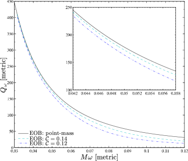
Stated differently, the function measures the number of GW cycles spent by the binary system within an octave of the GW frequency (it is therefore analogous to the “quality factor” of a damped oscillator). Let us also note that, in the stationary phase approximation, enters as an amplification factor of the signal, so that the squared signal-to-noise ratio is equal to Damour et al. (2000)
| (26) |
where denotes the amplitude of the time-domain metric waveform and where denotes the one-sided noise power spectral density and .
In view of its definition, is a useful quantitative indicator of the physics driving the variation of . Indeed, a change of of the order during a frequency “octave” corresponds to a local dephasing (around ) of rad. Because such a dephasing (if it occurs within the sensitivity band of the detector) can be expected to significantly affect the measurability of the signal, it is probably necessary to model with an absolute accuracy of about (see Ref. Damour et al. (2011) for a quantitative discussion of the admissible error level on in the BBH context).
We start our analysis by comparing the functions (as predicted by the EOB formalism) for the (metric) gravitational waveforms generated by three (equal-mass) binary models, namely a BBH and the two BNS systems discussed in Sec. II.1. To simplify the discussion, these functions are computed with the LO tidal interaction . [We will separately study below the effect of changing .]
Figure 3 compares the properties of the functions by showing together the curves for the three binaries versus their corresponding GW frequency. A number of remarks are worth making. First, is a large number that diverges in the small-frequency limit. This follows from the fact that in the limit one has , and then, via Eq. (24), . Second, the presence of tidal interactions decreases the “point-mass” value of by an amount that is (essentially) proportional to . In other words, tidal effects “accelerate” the inspiral by reducing the number of cycles spent around a given frequency. In particular, BBHs (which have vanishing tidal constants Damour and Nagar (2009); Binnington and Poisson (2009)) are effectively the binaries that spend the largest time at any given frequency. Finally, note that since is a large number, the fact that the curves look relatively close on the large-scale plot can be misleading, since the corresponding accumulated relative phase difference can actually be large (see inset, which shows that the absolute differences between the various is of order , corresponding to integrated dephasings of order radians).
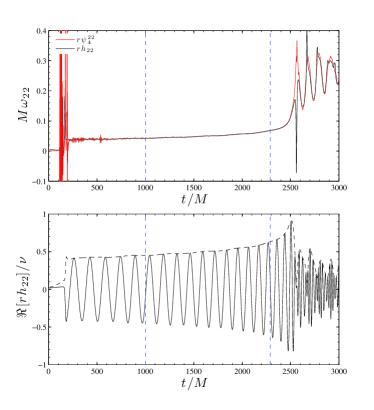
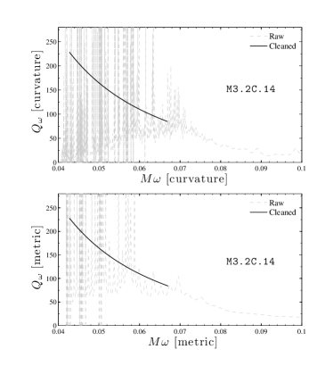
Although the calculation of the phase “quality-factor” is straightforward within the EOB framework, this is not the case when is to be calculated from the NR (either curvature or metric) waveforms. Indeed, the direct computation of the functions from raw data is in general made difficult by the presence of both high-frequency noise in and of low-frequency oscillations probably due to a residual eccentricity. This is illustrated in the right panels of Fig. 4, where we show with (light) dashed lines the raw NR functions obtained by direct time-differentiation of the NR curvature (top panel) or metric (bottom panel) phase for the binary M3.2C.14. A fourth order accurate finite differencing algorithm has been used to compute the derivatives. Similar results have been obtained also for the binary M2.9C.12.
The right panel of Fig. 4 shows that the two time-derivatives involved in the definition of amplify considerably the high-frequency noise contained in the NR phase evolution, and make it impossible to extract a reliable value of from such a direct numerical attack. To tackle this problem, one needs to filter out the high-frequency numerical errors in the time-domain phase before effecting any time-differentiation. To do this, we found useful to “clean” the phase by fitting the NR phase to an analytic expression that is inspired by the PN expansion. More precisely, after introducing a formal “coalescence” time and defining the quantity
| (27) |
we fitted the time-domain NR phase to an expression of the form
| (28) |
In this expression, we have set the lower coefficients and to and , as suggested by the corresponding lowest-order PN expression (see, e.g., Eq. (234) of Blanchet (2006)), but we left , , and the higher-PN ’s as free coefficients to be determined from the NR data. The basic idea is that of using a simple analytical form that incorporates the leading trend of to remove the influence of the numerical errors while leaving some flexibility in the subleading part of the phase evolution that is influenced by tidal effects. We view the fitting parameters as effective parameters for describing tidal-phasing effects.
Such a fit of the phase evolution can be reliably done only in a limited time interval. Indeed, one has to cut off both the early phase of the inspiral (where the numerical data is too noisy), and the last few cycles before the merger (where the PN-based fit is no longer a good approximation). We present in Appendix B a detailed discussion of the optimal choice of the time interval where to make the fit, as well as a series of consistency checks. See also the discussion at the end of Sec. V.2.
Let us start by discussing the application of this procedure to the GW phase (both curvature and metric) of the binary model M3.2C.14. The result of this fitting is shown by the solid lines in the right-panels of Fig. 4 (top, curvature phase; bottom, metric phase). The time interval on which we could reliably apply the fitting procedure is . This time window is indicated by the dashed vertical lines in the top-left panel of Fig. 4, were we show together the time evolution of both the curvature (dashed, red online) and metric (solid) GW frequencies. For completeness, the lower-left panel of the same figure translates this information in terms of GW cycles of the metric waveform. Note that this time interval excludes the first GW cycles (whose NR frequency is indeed seen to be quite noisy), but covers about GW cycles, and ends around GW cycles before the merger (defined as the maximum of the modulus of the metric waveform; the modulus of the metric waveform is indicated by a dashed line on the left-bottom panel of the figure). The corresponding frequency interval can be visualized on the right panels, and is listed in the fifth column of Table 3. Similar results are obtained also for the M2.9C.12 data (see Fig. 10 below). In this case, the time interval we use is , with the corresponding frequencies listed in the seventh column of Table 3. Finally, notice that for this model the inspiral is longer than in the previous case and so this interval actually corresponds to GWs cycles. In addition, similarly to the other case, our choice of fitting interval excludes the first GW cycles, and ends about GW cycles before merger.
As we will discuss below, although the frequency windows where our cleaning procedure allowed us to compute an estimate of the NR functions do not cover the full inspiral, these estimates will give us access to important information for performing quantitative comparisons with the predictions of the EOB (and Taylor T4) analytical models.
V Numerical Error-Budget
The aim of this section is to discuss the various errors affecting the numerical waveforms extracted (for both models) at and computed with the highest resolution. Such a discussion will in turn allow us to estimate an uncertainty range on the analytical parameter representing the not-yet-calculated, high-PN-order tidal effects entering the EOB description of the phasing.
We will discuss in turn the numerical errors entailed by three different effects: (i) the choice of EOS (isentropic versus non-isentropic evolution); (ii) the finite extraction radius; (iii) the finite resolution. We will perform this analysis both by comparing waveforms in the time domain and by means of the diagnostic.
V.1 Time-domain analysis
V.1.1 Non-isentropic evolutions
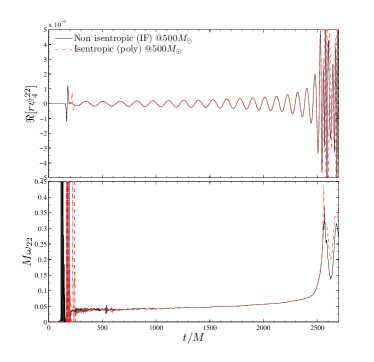
As discussed in Sec. II.1, we have evolved the binaries using either a (isentropic) polytropic EOS or a (non-isentropic) ideal-fluid EOS. We recall that, in the absence of large-scale shocks (like those taking place at the merger), the two EOSs are equivalent and should therefore yield evolutions that differ only at machine precision. In practice, however, when using the ideal-fluid EOS small shocks are produced in the very low-density layers of the stars even when these orbit Baiotti et al. (2008). These small shocks channel some of the orbital kinetic energy into internal energy, leading to small ejections of matter (i.e., amounting to a total of ), and are thus responsible for slight differences even during the inspiral. Since we are here presenting the results of simulations that are considerably longer than any presented so far and in particular of those in Refs. Baiotti et al. (2008, 2009a), it is important to quantify the influence of these non-isentropic effects. Concentrating on model M3.2C.14, we show in the top-panel of Fig. 5 the real parts of the waveforms computed with the two EOSs as extracted at . The bottom panel displays the corresponding instantaneous frequencies for completeness. As customary in comparing waveforms in the time domain, one allows for arbitrary relative time and phase shifts . These quantities can be determined in various ways, for example by means of the two-frequency pinching technique of Ref. Damour et al. (2008b). In this paper we find it useful to use the method used in Ref. Boyle et al. (2008) to compute . More precisely, given two timeseries of the phase defined on a given time interval that is covered by numerical points , with , we define the quantity
| (29) |
and determine and such that they minimize the “reduced” quantity
| (30) |
The minimization on is done analytically, while that on is done numerically. Note in addition that the square root of the minimum value of Eq. (30), say
| (31) |
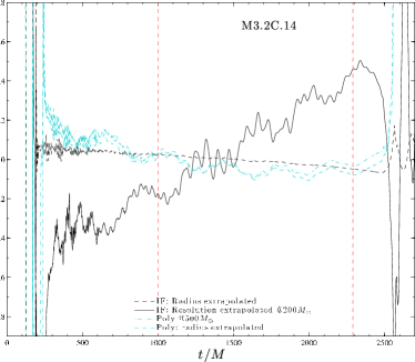
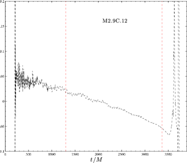
has the meaning of a root-mean-square deviation of the phase difference over the interval ; as such, it can also be employed to give a quantitative measure of a phase difference (and thereby of some phase errors).888We note in passing that the alignment procedure also highlights the weak dependence on the EOS of the late part of the waveform: although the inspiral of the non-isentropic waveform is about longer than the corresponding isentropic one, the growth of (and the corresponding phasing) is qualitatively and quantitatively very close for both models until peaks for the first time. The phase difference (least-square minimized on the time interval ) is represented as a dash-dotted line (solid light blue) in Fig. 6. One sees that the instantaneous phase difference varies roughly between rad and rad on this time interval, which corresponds to a “two-sided” Damour et al. (2008b) phase uncertainty of the order rad. The information of Fig. 6 is completed by Table 2, where we list the norm of the phase difference [i.e., the maximum absolute value of ], labelled , the root-mean-square as computed above, and the corresponding time interval that is used to compute . Note that gives a measure of the phase difference which is always significantly smaller than the norm. Indeed, these two quantities measure different aspects of a phase difference, and, when the time variation of is dominated by low-frequency effects (which can be roughly modelled as power laws), the averaging involved in the definition of will lead to a smallish ratio linked to integrals of the type .
V.1.2 Finite-radius extraction
We next discuss the phasing error introduced by the fact that our high-resolution target waveforms, for both models, are extracted at the finite coordinate radius . Note that, when expressed in units of the gravitational mass of the binary at infinite separation, this value corresponds to for M2.9C.12 and for M3.2C.14, i.e., , for one model waves are actually extracted slightly farther than for the other. For both models we have at our disposal several extraction radii, so that we can estimate the phasing error linked to the finite extraction radius as follows: (i) We used the raw data extracted at radii ; (ii) We time-shifted them so that this triplet of timeseries is expressed as a function of the (coordinate) retarded time ; (iii) We separated each curvature waveform in phase and amplitude as functions of (cf. page III.1); (iv) We fitted each resulting triplet of timeseries to a linear polynomial in the triplet of inverse extraction radii: . The quantities [i.e., and ] yield estimates of the amplitude and phase of the infinite-radius extrapolation of . We then compare the radius-extrapolated phase to the phase extracted at the outermost radius, allowing for additional time and phase shifts (which are determined by the least-square minimization discussed above).
The time evolution of the phase differences computed in this way are shown in Fig. 6 for model M3.2C.14 (top panel, dash-line) and for M2.9C.12 (bottom panel). This local information is completed by the “global” quantitative information (, ) listed in the last two columns of Table 2. On the basis of this analysis, we estimate that, for both models, the phase uncertainty due to finite extraction is of order rad almost up to the merger, i.e., roughly before the peak of the GW frequency.
| Model | EOS | Extrap. | ||||
|---|---|---|---|---|---|---|
| [rad] | [rad] | |||||
| M3.2C.14 | IF | radius | ||||
| M3.2C.14 | IF | resolution | ||||
| M3.2C.14 | poly | |||||
| M3.2C.14 | poly | radius | ||||
| M2.9C.12 | IF | radius |
V.1.3 Finite-resolution error
Finite-resolution errors have already been discussed in detail in our previous work Baiotti et al. (2009a), which used the same numerical setup (i.e., the same resolution and grid structure) adopted here. Skipping the details, we recall that it was shown there that, at the resolution that we are using in this work, the dynamics and waveforms are in a convergent regime, with a convergence rate that is during the inspiral phase and drops to after the merger, when large-scale shocks appear. As the computational cost of the calculations presented here is already at the limit of what can be reasonably afforded, we have decided to estimate the truncation-error of our present waveform by assuming that the inspiral convergence rate found in our previous work Baiotti et al. (2009a) approximately holds in the present (numerically similar) case. We have then selected the more compact binary M3.2C.14 and used only two simulations with different resolutions. More specifically, we have considered a “high-resolution” simulation, where the finest refinement level has a resolution , and a “low-resolution” simulation, with . For this particular comparison the waveforms are extracted at . When comparing the low- and high-resolution curvature waveforms, after suitable alignment, one discovers that the phase difference accumulated between the two resolutions over a timescale of during the inspiral is about rad (corresponding to a relative error of ). Using the convergence rate discussed above, we can now Richardson-extrapolate the results obtained with the two resolutions and obtain an estimate of the “infinite-resolution” waveform. More precisely, we model the suitably aligned, low- and high-resolution phase evolutions as
| (32) | ||||
| (33) |
where represents the infinite-resolution phase (). From the above equations, we obtain the following estimate of the infinite-resolution extrapolation of the phase evolution
| (34) |
| Model | EOS | Extrap. | ||||||
|---|---|---|---|---|---|---|---|---|
| [] | [rad] | [] | [%] | |||||
| M3.2C.14 | IF | |||||||
| M3.2C.14 | IF | radius | ||||||
| M3.2C.14 | IF | resolution | ||||||
| M3.2C.14 | poly | |||||||
| M3.2C.14 | poly | radius | ||||||
| M2.9C.12 | IF | |||||||
| M2.9C.12 | IF | radius |
We performed the same extrapolation also on the waveform modulus, so as to have access to the complete extrapolated curvature waveform. The solid line in Fig. 6 displays the phase difference . This indicates a phase uncertainty of rad on as measured up to about before the maximum of . See Table 2 for the corresponding global measures of the phase uncertainty, and . Note that these uncertainty estimates are much larger than those normally computed for binary BH simulations for the same computational costs (see, for instance, Pollney et al. (2009)). This is the natural consequence of the smaller resolution employable here and of the lower-order convergence that one achieves when solving the hydrodynamics equations. Since this error is deduced only after assuming a certain convergence order (in addition obtained from a slightly different numerical setup) it will be used below only to estimate a rough uncertainty range on the value of the higher-order EOB tidal correction parameter . We will comment more on this in the next Sections.
Adding in quadrature the various uncertainties computed so far to obtain a total error bar on the phases of the data for the M3.2C.14 model would give a (two-sided) time-domain phase uncertainty rad, when excluding the uncertainty due to the finite resolution, or rad when including it. Alternatively, if we add in quadrature the root-mean-squares of the corresponding phase errors we find rad, when excluding the uncertainty due to the finite resolution, and rad when including it. Clearly the resolution-extrapolation error is dominating the error budget. In view of the uncertainty in estimating this source of error, we will not directly use these time-domain phase-error levels in estimating the uncertainties in the comparison between the EOB, T4, and NR phasings. As we will discuss next, we prefer to express the information gathered above on numerical errors in terms of the corresponding curves.
V.2 analysis
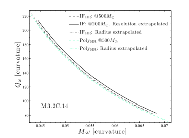
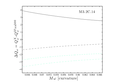
In Sec. IV we have introduced as a convenient, intrinsic diagnostics to describe the phasing of the waveform. In particular, it allows us to better visualize the influence of tidal effects on the phasing, as well as to compute the dephasing accumulated on a given frequency interval. It is then useful to recast the various time-domain phase uncertainties on the high-resolution waveform extracted at discussed above, in terms of . In practice, we apply the cleaning procedure on each waveform of Table 2 so as to obtain four curves. These curves are displayed together in the left panel of Fig. 7, while the fifth column of Table 3 lists the specific frequency intervals that were selected to apply the cleaning procedure. For a quantitative assessment of the differences between the curves, we present in the right panel of Fig. 7 the quantity , where the labelling indicates any curve other than our fiducial one, . Although the information conveyed by this figure is qualitatively analogous to the time-domain analysis, Fig. 6, it is made here both independent of any phase-alignment procedure and simpler to quantify. First of all, the figure shows that the extrapolations in radius and in resolution act in different directions: the first one pushes the curve down (i.e., less GW cycles accumulated on a given frequency interval, tidal effects look stronger), while the second one pushes the curve up (i.e., more GW cycles accumulated and tidal effects look weaker). This result is qualitatively compatible with the corresponding curves in Fig. 6, whose slopes have opposite signs. In addition, by integrating in frequency the curves on the common frequency interval one obtains an estimate of an actual accumulated phase error that can be compared to our previous time-domain results (i.e., Fig. 6). The result of this integration is given in the seventh column of Table 3. Note that the computed in this way is typically significantly larger than what was estimated above in the time domain. For instance, regarding the comparison with the resolution extrapolated waveform, the -based procedure indicates a phase difference of about 1.3 rad over ; by contrast, inspecting Fig. 6, where the vertical (red) dashed line corresponds to in the time-domain, we read from the plot an accumulated phase difference on this interval of about 0.8 rad, i.e., about smaller. Similar results hold for the other phase comparisons. This increase in the estimated phase errors is probably due to the additional uncertainty brought by the necessity to use a phase-cleaning procedure to compute each (see below). This is the price we have to pay to be able to have the convenience of an intrinsic diagnostic of the phase evolution.
A separate discussion is needed when comparing isentropic and non-isentropic curves. Figure 7 indicates that the curve corresponding to the ideal-fluid EOS lies above the polytropic one, and this indicates that the tidal interaction appears weaker in the former case than the latter (because the curve referring to the ideal-fluid is closer to the point-mass curve than the polytropic curve, see below). This effect was already discussed in Ref. Baiotti et al. (2008) and is likely due to the small shocks that are formed by the interaction between the outer layer of the stars and the external atmosphere. The polytropic EOS should yield a priori a more accurate evolution during the inspiral, when the stars are far apart, but should become progressively inaccurate and inconsistent when the two stars become closer and closer, with mass shedding and the formation of actual shocks that are not simply due to the weak interaction with the atmosphere. For this reason we will not use the isentropic ’s as a lower bound in our analysis, but we will focus only on non-isentropic evolutions, though keeping in mind that there is a further source of error on them.
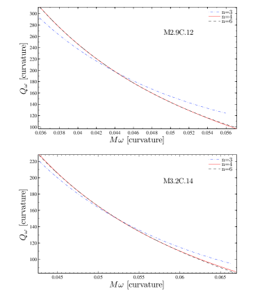
A natural question that comes at this stage is: what is the uncertainty on the determination of the function that is due to the phase-cleaning (i.e., phase-fitting) procedure? A first way of addressing this issue is to measure the impact that changing our fiducial fitting function Eq. (28) has on . Focussing, for both models, only on our basic data, we computed the cleaned frequency using, besides our fiducial fitting polynomial of order (see Eq. (28)), either a lower-order polynomial truncated at or a higher-order one, extended up to .999Note that is not meaningful as the corresponding term is exactly degenerate with . Furthermore, the use of does not help, as the corresponding term is nearly degenerate with . The results of these computations are displayed in Fig. 8 for model M2.9C.12 (top panel) and M3.2C.14 (bottom). The results are qualitatively analogous in the two cases. First, we see that the low polynomial order is clearly too small, and fails to capture (when comparing it to the PN or EOB curves, which are accurate on the low-frequency side) the low-frequency behavior of . By contrast, the fact that the curve is barely distinguishable (on the scale of the figure) from the one is an indication of a sort of “convergence” of our fitting procedure as the number of powers is increased. We can therefore use the difference between and as an estimate of the uncertainty entailed by the cleaning procedure. Computing this difference, we find that it remains of order unity all over the fitting frequency interval . In conclusion, we estimate the uncertainty associated with the choice of the order of the fitting polynomial to be . Note that this error is rather small compared to the various numerical errors on displayed in Fig. 7, but it is only a lower bound on the uncertainty level linked to the cleaning procedure.
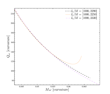
In particular, another relevant source of uncertainty on is the choice of the fitting time interval . In Appendix B we explicitly discuss some rules of thumb that we follow to select such that the cleaning procedure is reliable and robust. To complete the discussion of Appendix B, we investigate (for model M3.2C.14) the modifications in brought by changes in the choice of . More precisely, we modified the right-end point of our preferred cleaning time interval (see Table 3) by (with fixed polynomial order ). The three curves corresponding to are displayed in Fig. 9. When comparing the cases , we find that the absolute value of the difference in stays all over the time-interval (corresponding to a frequency interval ), but then grows up to values of order near . On the other hand, when comparing the cases we find that the absolute value of the difference in stays of order all over . This further analysis suggests that the cleaning procedure allows us to determine within an uncertainty level during most of the inspiral, with a possible increased uncertainty level near the end of the inspiral. Note that these levels are significantly smaller than the changes in the analytical ’s associated to a variation of the NNLO parameter between and (see next Section).
VI Comparison of analytical and numerical-relativity results
VI.1 Characterizing tidal effects from NR simulations
Before proceeding with the NR/AR comparison it is useful to discuss a procedure by means of which it is possible to effectively subtract the tidal interaction from the NR curves obtained so far. This procedure will then allow us to obtain a phase diagnostic that, within some approximation, represents a non-tidally interacting binary, namely a binary of two point-particles. As pointed out in Ref. Damour and Nagar (2010), the binding energy of a binary system is approximately linear in and it is therefore possible to subtract the tidal effects by combining different sets of binding-energy curves coming out of NR calculations. In particular, Ref. Damour and Nagar (2010) computed several “tidal-free” binding energy curves (one curve for each combination of two different data sets) that were compared with the corresponding point-mass curve computed within the EOB approach or within non-resummed PN theory. This procedure allowed for both the identification (and thus subtraction) of systematic uncertainties in the NR data and the discovery of higher-order tidal amplification effects.
Here we will generalize the approach introduced in Ref. Damour and Nagar (2010) to the curve. In particular we assume that the function is approximately linear in the (leading) tidal parameter , at least during part of the inspiral, say up to some maximum frequency (we will use ). As a result of this assumption, we can approximately write , for each binary, as
| (35) |
where is an index labelling some binary system. As a result, given the diagnostics of two different binaries with labels , we can estimate the two separate functions and as
| (36) | ||||
| (37) |
From the decomposition (35), we see that, by definition, the function denotes the diagnostic of two non-tidally interacting NSs, namely of two point-like (relativistic) masses (and also two BHs Damour and Nagar (2009); Binnington and Poisson (2009)). Hence, the function is seen to represent, within the present approximation, the effect of the tidal interaction on the function. The calculation of both functions contains therefore important information about the analytical representation of tidally-interacting binary systems. In the following we will only discuss the computation of the tidal-free part , leaving a discussion of the properties of to a future work.
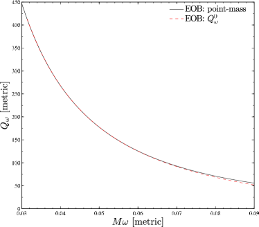
This subtraction procedure for computing can be first tested by using the EOB metric waveforms computed from binaries with compactnesses and . The result of the subtraction is displayed in Fig. 10, where we compare the point-mass (i.e., BBH) EOB curve (solid line) to the curve (dashed line), obtained by inserting in Eq. (36) the and data of Fig. 3. The fact that the curves are barely distinguishable up to (where the difference is ) gives us confidence that the procedure will be effective also with actual NR data. This will indeed be shown in the next Section.
VI.2 Inspiral: subtracting tidal effects from NR data
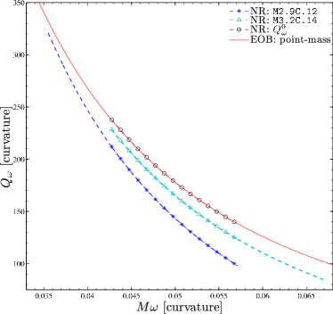
We start our NR/AR comparison by computing the function as defined by Eq. (36) from NR data using our two models M2.9C.12 and M3.2C.14 as the binaries labelled g and in that equation. For all the comparisons carried out here we have limited ourselves to using the curvature waveforms, although similar results can be obtained from the corresponding metric waveforms.
The results are shown in Fig. 11, which reports four different curves: the two tidally-modified NR curves for the binaries M2.9C.12 and M3.2C.14 (with the asterisks and triangles highlighting a sample of the data on the common frequency window), the subtracted NR curve (with empty circles), and the point-mass-EOB (as a solid line). This figure illustrates at once several of the main results of this paper. First of all, it highlights the excellent agreement between the cleaned NR and the analytical EOB one (cf. the red solid curve and the empty circles). This gives evidence both for the validity of the EOB description and for the robustness of our cleaning procedure. When we compute the relative phase difference over the common frequency interval , we obtain the remarkably small value of rad, which translates into a relative difference 101010To cross-check the consistency of both the recovery procedure of from and the cleaning of the phase, we carried out the same calculation also for the metric waveforms, finding a difference rad, which is consistent with the estimated error-bar rad on the EOBNR point-mass waveform during inspiral Damour and Nagar (2009a).. Second, it confirms, independently of our EOB-based check (cf. Fig. 10), that the NR tidal effects are approximately linear in at least in the early part111111In the following, we will refer to the frequency domain as the “early-inspiral”. Note that for a fiducial system corresponds to Hz. Note also that in the case, for instance, of our system the frequency is reached at time , i.e., only about GW cycles before merger. of the waveform, and thus that they can be efficiently subtracted. Third, it illustrates the fact that the tidal interaction between the two objects is important already in the early-inspiral part of the waveform, since both the M2.9C.12 and M3.2C.14 curves are significantly displaced (by ) with respect to the point-mass one. Fourth, such a good agreement with the point-mass EOB analytical model (which was tuned so as to accurately reproduce the equal-mass BBHs) yields an independent check of the consistency and accuracy of our numerical simulations. Finally, we note that in Ref. Damour and Nagar (2010) the procedure of subtraction, applied there to the NR binding energy, was giving a curve slightly displaced with respect to the point-mass EOB (or PN) curve. This displacement was interpreted as evidence of systematic errors in the NR simulation and prompted the introduction of a “correcting” procedure, which however is not necessary for the present NR data.
VI.3 Early inspiral: evidence for large NNLO tidal effects
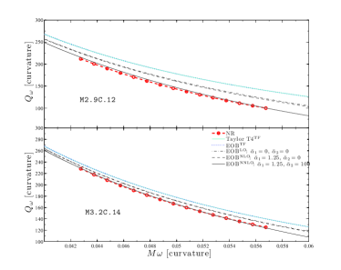
We continue our analysis by focussing on the influence of LO tidal effects on the early-frequency part of the curves. We already know from Fig. 11 that tidal effects are important in such early-frequency part of the simulations, since we found a significant difference (of order ) between the point-mass curve and the NR ones. Can these differences be accounted just by the LO tidal effects? Figure 12 shows quite clearly that this is not the case and that the LO description is not sufficient to match the corresponding NR curves (dashed line with open circles). Note that this is the case for both the M2.9C.12 (upper panel) and the M3.2C.14 binaries (lower panel). The difference with NR data (on the frequency interval where the data of M2.9C.12 and M3.2C.14 overlap) is quantified in the first line of Table 4 and is rather large, namely several radians.
We next turn to analyzing the effect of NLO and NNLO tidal interactions. Here, we will regroup under the label of NLO both 1PN and 1.5PN effects. As seen in Fig. 12, the inclusion of the NLO tidal effects ( Damour and Nagar (2010), 1PN tidal-radiation effects Vines et al. (2011), and 1.5PN tail effects) has only a barely noticeable effect on the curve. This clearly indicates the need for large NNLO (2PN and higher) tidal effects, which we chose to parameterize by means of the effective parameter introduced in Eq. (14). We then found that choosing yields a good match between the NR and EOB curves (solid line, EOBNNLO), especially for the M3.2C.14 model, for which the analytical curve is on top of the NR data. See also Table 4 for the corresponding phase differences. The Table also indicates that if we use , as we did in Ref. Baiotti et al. (2010), the accumulated dephasing on the common frequency interval is further reduced to a fraction of a radian for both models. Note that the implementation of the EOB waveform and radiation reaction that we use here is slightly different with respect to the one of Baiotti et al. (2010), which was based on Ref. Damour and Nagar (2010) and thus did not incorporate the waveform 1PN corrections Vines et al. (2011) nor the tail effects. This explains why we were quoting different phase differences ( rad) over the same interval when referring to in Baiotti et al. (2010). However, we prefer here the smaller value because the corresponding curve is, on average, closer to the NR one on the larger frequency interval on which we succeeded to clean the NR phase.
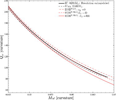
It is important to recall that various numerical errors affect the computation of the NR curves, and thereby affect the quantitative determination of the effective NNLO parameter . For example, we have seen that the resolution extrapolation (which seemed to be the dominant source of uncertainty) has the practical effect of pushing the numerical curve upwards. This suggests that the value obtained from using finite-resolution NR data is probably too large. To have a rough idea of the error range on , we compare in Fig. 13 various NR and EOB curves. More precisely, this figure shows two numerical black curves: a solid one, derived from our fiducial highest-resolution and largest-extraction-radius , and a dashed one, derived from the resolution-extrapolated NR data. Also reported in Fig. 13 are three analytical curves (red lines): namely the EOB predictions for the three values , respectively. Clearly, the resolution-extrapolated curve is close to the analytical curve corresponding to the value , which is more than twice smaller than the value suggested by our fiducial, highest-resolution NR data. It is interesting to note that the value agrees with the preferred value of (when using ) found in Damour and Nagar (2010), the work that pinpointed the first evidence for the need of large NNLO effects. Let us also note that, independently of the precise value of , Fig. 13 clearly shows the need for large NNLO effects, namely .
Let us also recall that the other sources of numerical error act in various directions. For instance, non-isentropic effects actually act so as to effectively reduce the magnitude of the tidal interaction121212Indeed the non-isentropic curve lies above the isentropic one. This is certainly a source of error during the early-inspiral, where the isentropic description is a priori more accurate but some energy is channelled by shocks due to the interaction with the atmosphere., while the extrapolation to infinite extraction radius acts in the opposite direction, namely effectively increasing the magnitude of the tidal interaction.
In view of our incomplete knowledge of all the sources of error intervening in our NR waveforms, we can only conclude that probably lies in the range , with the understanding that the lower values () are preferred because of the expected importance of the truncation error in the numerical simulations. More numerical simulations with a more detailed estimate of the numerical error budget will be needed in the future to reduce this error range on .
| Model | NNLO | ||
|---|---|---|---|
| parameters | [rad] | [rad] | |
| EOBLO | |||
| EOBNLO | |||
| EOBNNLO | |||
| EOBNNLO | |||
| T4LO | |||
| T4NLO | |||
| T4NNLO |
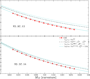
Let us conclude this Section by briefly discussing the comparison between the NR diagnostics with those obtained using several versions of the Taylor-T4 approximant. More precisely, Fig. 14 displays the following curves: the tidal-free T4 model (, dotted line), the LO Taylor-T4 model (dashed-line), the NLO (i.e., 1PN) one (dash-dotted line), and finally the effective NNLO one (solid line), as introduced in Sec. III.3 above. Let us recall that the NNLO model contains an effective 2PN parameter, called , which is a rough T4 analog of the NNLO EOB parameter and which enters the T4 tidal amplification factor Eq. (23). Similarly to the EOB case, one finds that a suitably large value of the effective 2PN tidal parameter can provide curves that are close to the numerical ones. The integrated dephasings corresponding to Fig. 14 are listed in Table 4.
A few comments are worth making on the comparison between the EOB and T4 results. Let us first recall that, in the BBH case, it has been shown that the EOB description is definitely more accurate than the Taylor-T4 one, especially when considering unequal mass ratios Damour et al. (2008a) or spin effects Hannam et al. (2008). However, as we are considering here an equal-mass case and frequencies that are smaller (when considering the dimensionless frequencies ) than in the BBH case, the tidal-free T4 phasing is quite close to the EOB one (see Fig. 12). Concerning tidal-extended models, we see that both EOB and T4 approximations highlight the need for large higher-order tidal-amplification factors. When choosing one such amplification factor for both BNS systems (say for EOB and for T4), a close look at the comparison of the corresponding curves suggests that the EOB-predicted curves are somewhat closer than the T4-predicted one to the NR curves. However, this, by itself, would only be a weak indication that EOB gives a better representation of our fiducial NR data, especially in view of the large uncertainties discussed above on the actual value of the functions. On the other hand, we consider that the need of a much larger tidal-amplification factor in the T4 case is an indication that the analytical modelling of (LO, NLO and NNLO) tidal effects within the EOB-resummed framework might be more robust than the corresponding one based on Taylor-expanded approximants. Indeed, in both cases the parametrization of NNLO effects involves multiplying tidal effects by a factor having a similar structure: versus . In addition, the quantities and are numerically close to each other (both being close to ). At the end of the inspiral, reaches numerical values of order (i.e., Hz for a fiducial BNS system), corresponding to . For such a value one sees that the EOB amplification factor (with ) remains relatively moderate131313For , this amplification factor becomes , namely , while the T4 one (with ) is suspiciously large, and is completely dominated by the 2PN contribution, namely . Another way to phrase this is to notice that the large T4 value is such that the 2PN contribution starts dominating the LO term at , i.e., at large separations corresponding to rather low frequencies , i.e., Hz for a fiducial BNS system. Furthermore, such a large value for works well for binary M3.2C.14, but less well for binary M2.9C.12.
Clearly, in view of the large current uncertainties on the NR curve, more work is needed to confirm this provisional conclusion. In particular, more accurate NR simulations, encompassing more compactnesses and different mass ratios will be needed to assess the relative merits of the EOB versus the Taylor-T4 description of tidally interacting BNS systems.
VI.4 EOB/NR phasing
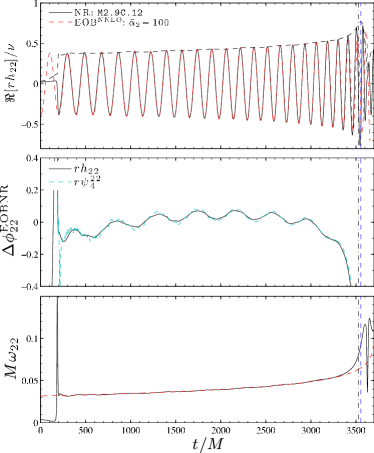
So far our NR/AR comparison based on the function has been limited to a frequency interval which did not cover the last octave of frequency evolution, even if, when viewed in the time domain, this interval covered most of the cycles of the inspiral. In this section we finally focus on a phasing comparison in the time domain which covers the full inspiral and plunge phase, up to the merger of the two NSs. Our strategy here will not be to explore from scratch a good range of values of the tidal NNLO parameter values, but instead to use the value suggested by our previous -analysis, and to explore to what extent it succeeds in providing a waveform which agrees with our fiducial (highest-resolution) NR waveform over the full inspiral. Anticipating our conclusion, we will find that the EOB waveform with does closely agree (both in phase and modulus) with the NR waveform essentially up to the merger.
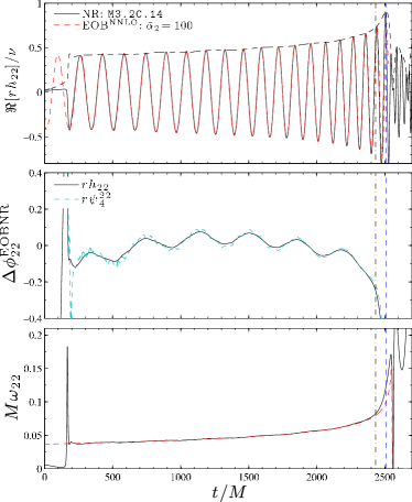
This is shown in Fig. 15, which compares the (real part of the) EOB and NR metric waveforms for the case including NNLO effects with . The left panels refer to the M2.9C.12 binary, while the right panels refer to the M3.2C.14 one. The top panels show the real parts of both the EOB and NR waveforms (divided by the symmetric mass ratio ); the middle panels display instead the corresponding phase differences , for both metric (solid line) and curvature (dashed line) waveforms, for completeness; the bottom panels compare the EOB (dashed line) and NR (solid line) instantaneous GW frequency. The least-squares phase alignment has been performed on the time interval for the M2.9C.12 binary and for the M3.2C.14 one.
The two vertical lines (dot-dashed and dashed) indicate the “end of the inspiral phase”, as defined either within the EOB analytical framework (dot-dashed line) or by using NR information (dashed line). Note that we call here simply “inspiral” what was called “insplunge” in previous EOB studies, namely the union of the inspiral and (when it is reached before merger) of the plunge. More precisely, the dashed line indicates the NR-defined “merger”, i.e., the time (computed from the NR data) at which the modulus of the metric waveform reaches its first maximum. On the other hand, the vertical dash-dotted line indicates the EOB-defined “contact” between the two NSs141414Note that the styles of the corresponding merger and contact vertical lines as depicted in the two panels of Fig. 2 of Ref. Baiotti et al. (2010) are inverted with respect to the text there. See the arXiv version for the correct figures.. Such a formal contact moment was introduced in Eqs. (72) and (77) of Ref. Damour and Nagar (2010), by a condition expressing that the EOB radial separation becomes equal to the sum of the tidally deformed radii of the two NSs, namely
| (38) |
where is the dimensionless parameter controlling the (LO) strength of the tidal deformation of the NS labeled by its companion and where is the shape Love number Damour and Nagar (2009); Damour and Lecian (2009). A recent study of the tidally induced shape deformation of BHs Damour and Lecian (2009) has shown that the BH shape Love number was a function of the separation , which increased as decreased (and increased). This behavior is similar to the behavior of the (effective) quadrupole Love number , where both and were found to be positive Damour and Nagar (2010). One would need a special study devoted to the comparison of the EOB-predicted NS shape deformation to NR data to investigate in detail the dependence of the analogous . Leaving to future work such a study, we will here replace the -dependent effective shape Love number by a constant, chosen such that the EOB-predicted contact happens before the NR-defined merger for the two BNS systems we consider. We found that works, and this is the value we will use to replace and in the contact condition written above151515A similar approach was taken in Damour and Nagar (2009); Baiotti et al. (2010), with a less conservative value . Let us recall that the computation of the infinite-separation shape Love number of NSs gives values of order unity Damour and Nagar (2009).. An important point to note is that our (EOB-based) analytical definition of contact allows one to analytically predict a complete inspiral waveform, including its termination just before merger.
Figure 15 shows that the agreement in the time domain between the analytic EOB description and the fully numerical one is extremely good essentially up to the merger. More precisely, the match between the two descriptions is excellent both in modulus and in phase, with a dephasing of order rad during most of the long inspiral phase. It is only during the last before contact that the dephasing grows significantly. One should note that this excellent EOB/NR agreement holds for both binaries M3.2C.14 and M2.9C.12, and has been obtained by tuning a single tidal-amplification parameter.
Clearly the results presented here give only a first cut at these issues. More NR/AR comparisons are needed to confirm our findings and to determine the most effective value of . With sufficiently accurate NR data one can hope to determine not only the effective tidal-amplification factor , but also the precise separation-dependence of . This would allow one to extend the EOB description right up to the merger.
VII Conclusions
We have presented the first comprehensive NR/AR comparison of the gravitational waveforms emitted during the inspiral of relativistic BNSs as computed via state-of-the-art numerical-relativity simulations and as modelled via state-of-the-art analytical approaches. Overall, the work reported here and our findings can be summarized as follows.
-
1.
We have considered the longest to date numerical simulations of inspiralling and coalescing equal-mass BNSs modeled either with an ideal-fluid or a polytropic EOS. Because tidal effects are most sensitive to the stellar compactness, we have considered two binaries with either a small compactness of or with a large compactness of . The parts of the waveforms relative to the inspiral cover between and cycles and have been studied to isolate possible sources of error, such as non-isentropic evolutions, finite-radii GW extractions, and the use of finite resolutions. For the model with the highest compactness, the first two sources of errors lead to a total error-bar in the GW phase of rad, while the error coming from a finite resolution indicates an accumulated phase error of rad.
-
2.
We have used the function as a useful diagnostic of the physics driving the evolution of the GW frequency . The calculation of this quantity is however challenging when made from the early-inspiral part of the NR waveforms, as the latter is affected by a series of contaminating errors. We have filtered out these errors by fitting the NR phase evolution with a simple analytical expression that reproduces at lower order the behavior expected from the PN approximation. We have compared the various ’s obtained from different data to estimate the error range entailed by comparing analytical predictions to our highest-resolution, largest-extraction-radius NR data.
-
3.
Using the estimated function we have shown that it is possible, at least for frequencies (i.e., Hz for a fiducial BNS system), to subtract the tidal-effect contribution from the NR waveforms and consistently match this with the expected EOB model for point particles which has been successfully matched to BBH simulations. The ability to perform this match accurately provides us with an independent validation of the quality of our numerical results as well as with a confirmation that the function is approximately linear in the (leading) tidal parameter .
-
4.
The comparison of analytical predictions with NR data shows that tidal effects are significantly amplified by higher-order (NNLO) relativistic corrections even in the early inspiral phase. These NNLO tidal corrections are parameterized within the EOB approach by a unique (effective, 2PN) tidal parameter . Although the most precise available at the moment, the quality of the NR data is such that we can only constrain the actual value of to be in the range .
-
5.
Once a single choice for is made, the EOB-predicted waveforms agree (both in phase and in modulus) with the NR ones (for both BNS systems) within their error bar and essentially up to the merger.
-
6.
Finally, we have also compared the NR phasing with the one predicted by a non-resummed Taylor-T4 PN expansion, completed by additional tidal terms. If one uses only the currently known analytic T4 tidal terms, the T4 model dephases (when ) by more than rad already at the GW frequency , which is about twice smaller than the GW frequency at merger (we recall that corresponds to Hz for a fiducial system). On the other hand, a good match (for both compactnesses) with the NR phasing is possible if one allows for a T4 analog of the EOB parameter, i.e., an (effective) 2PN amplification of tidal effects. The corresponding parameter is suspiciously large, works well for binary M3.2C.14 but less well for binary M2.9C.12, and dominates the amplification of tidal effects already at frequencies (corresponding to Hz). This seems to suggest that the EOB-based representation of tidal effects is more reliable than the Taylor-T4 one.
In summary, the work presented here opens new avenues to the important synergy between numerical and analytic descriptions of inspiralling compact-object binaries in general relativity. For the first time we have shown that an analytic modelling is possible also for objects which cannot be treated as point-particles and for which, therefore, tidal effects represent important corrections. Although the results presented here are very encouraging, a number of improvements are needed on both the numerical and the analytical sides. On the numerical side, higher resolutions and better measures of the convergence rates (which are particularly challenging in non-vacuum simulations) are needed to decrease the numerical phase errors to and reach firm conclusions about the tidal contributions to the phasing. On the analytical side, higher-order PN calculations are needed to better determine the form of the NNLO corrections. Both of these goals will be the subject of our future work. Hopefully, progress on both fronts will enable us to determine the crucial tidal-induced dephasing function with an accuracy sufficiently high to extract reliable information on the EOS of matter at nuclear densities 161616Simple estimates based on the scaling suggest that one needs to know with a fractional accuracy better than to constrain NS radii to a relative precision of . See also Ref. Pannarale et al. (2011) for the prospects from a BH-NS system..
Acknowledgements.
We are grateful to Sebastiano Bernuzzi for discussion throughout the development of this work and to Francesco Pannarale for useful input. The simulations were performed on the Ranger cluster at the Texas Advanced Computing Center through TERAGRID allocation TG-MCA02N014, and on the cluster Damiana of the AEI. This work was supported in part by the DFG Grant SFB/Transregio 7, by “CompStar”, a Research Networking Programme of the European Science Foundation, by the JSPS Grant-in-Aid for Scientific Research (19-07803), by the MEXT Grant-in-Aid for Young Scientists (22740163), and by NASA Grant No. NNX09AI75G.Appendix A Computing metric waveforms from
We discuss here the details of how to accurately derive the metric waveforms from the numerically computed curvature waveforms . We first recall that the procedure outlined in Ref. Damour et al. (2008a) consisted essentially of three steps. (i) First one performs the double integration of starting at with the integration constants set to zero; this amounts to defining
| (39) | ||||
| (40) |
The provisional metric waveform differs from the “exact” metric waveform (6) (integrated from past infinity) by a linear function of , say
| (41) |
(ii) The second step consists in obtaining an estimate of the two (complex) integration constants () that enter the metric waveform (6) by fitting over the full simulation time interval the -integrated waveform (40) to a linear function of , say , where and are complex quantities. (iii) The third and final step of the procedure of Ref. Damour et al. (2008a) consisted in subtracting the linear function from so as to define an approximation to the ()-integrated metric waveform, say .
Here we will use a “new” (three-step) procedure, which starts with the same step (i), but modifies both steps (ii) and (iii) so as to get a better approximation to the exact metric waveform. First of all, we define an “adiabatic-like” approximation to the metric waveform,
| (42) |
and use this to define
| (43) |
As is approximately equal to (because of the approximately adiabatic nature of the inspiral), we see from Eq. (41) that will be closer to the unknown linear function than was. Therefore, the next step is to perform the linear fit on this rather than on itself. Then, the last step (iii) consists, as in the past, in subtracting the resulting improved linear fit from the (–integrated metric waveform .
In addition, let us note that we perform the fit not on the whole time interval, but rather on a restricted time interval that cuts away the first cycles of the waveform. Finally, after doing several tests, we realized that the entire procedure leads to a physically more reliable metric waveform (see below) if is fitted not to a simple linear function, but rather to a quadratic171717We think that such a quadratic fit is needed for absorbing several effects that “pollute” the waveform, notably finite-extraction-radius effects, remnant junk radiation, etc. In this respect, we also mention that Ref. Baiotti et al. (2009b), in the context of non-spherical star oscillations, found that a quadratic polynomial used in the recovery of from was a necessary choice to find a good agreement both with Abrahams-Price metric extraction and perturbative waveforms. one, .
As emphasized in Ref. Damour et al. (2008a), we accept the integrated waveform if and only if its modulus exhibits a monotonic growth in time during the inspiral, consistently with the expected circularly polarized behavior of the metric waveform (as well as the curvature one)181818Note however that small-amplitude, high frequency “ripples” are still present in the modulus. Their origin is however essentially numerical, as they are also present in the modulus of .. Figure 2 displays the metric waveforms (both for the M2.9C.12 (left) and the M3.2C.14 (right) models) obtained using this improved procedure. The time intervals where we fit the waveforms to get start respectively at (model M2.9C.12) and at (model M3.2C.14). Note how the modulus of both models exhibits a smooth monotonic behavior in time.
Appendix B Cleaning the GW phase and curves
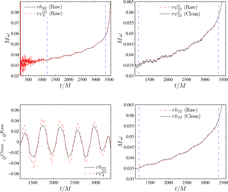
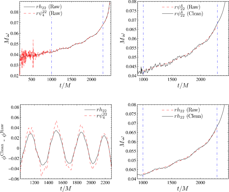
We next provide more detailed information about the cleaning procedure of the NR GW phase advocated in Sec. IV and used to drive NR/AR comparisons. As we said in the main text, the final goal is to fit away the high-frequencies oscillations in the GW phase so as to get a clean and smooth curve, Eq. (24). We recall that the idea is to fit with an analytic expression that is modeled on the PN expansion. Defining the quantity
| (44) |
one then fits the NR phase with an expression of the form
| (45) |
where , , and the ’s are free coefficients to be determined by the fit. Note that can be thought of as defining a formal “coalescence” time. There are two delicate (correlated) points: (i) how many powers of [possibly including also terms] one has to include in Eq. (45), and (ii) on which (time) interval the approximate description of given by Eq. (45) (and consequently of ) is reliable. The procedure to select the “best” time interval and to consistently assess the quality of our cleaned curves can be summarized as follows:
-
1.
The initial time is chosen so as to eliminate as much as possible the most noisy part of the curvature frequency. In practical terms, this meant cutting at for M2.9C.12 data and for data. This is illustrated in the top-left panels of Fig. 16 (for M2.9C.12 data) and of Fig. 17 (for M3.2C.14 data), which show the curvature (dashed line) and metric (solid line) instantaneous GW frequency . In both plots, the first vertical line identifies the location of .
-
2.
For a given order of the polynomial, we found the right end, , of the time window essentially, by trial and error, monitoring the behavior of several quantities. In particular, (i) we checked that the cleaned visually “averages” the raw , for both and data. This is illustrated in the top-right and bottom-right panels of Figs. 16-17, the raw data appearing as dashed lines, the cleaned data as solid lines. Then, (ii), we require that the phase difference averages to zero, which indicates that we have subtracted all the “secular” trends by means of our polynomial fit. The quantity (both curvature and metric) is displayed in the bottom-left panel of Figs. 16-17. The fact that it averages to zero is the indication that our fit caught the “secular” behavior of the phase, averaging away both (numerical) low-frequency and high-frequency oscillations.
-
3.
For a fixed time window, the inspection of is also crucial for choosing the order of the polynomial in , which we set to be of fourth-order. A 3rd-order one is clearly not enough to get the right trend of the frequency (and thus of ) up to the end of our preferred interval.
-
4.
To better select the end of the time window, we found it useful to monitor the difference between the curvature and metric ’s, namely . We typically choose the value of in such a way that is always smaller than on the frequency interval corresponding to . This value can be estimated by comparing curvature and metric ’s within the EOB. For example, for the NNLO model with one checks that when for , and when for . This gives us an idea of the level of that we can accept from our cleaned NR curves, so that we can choose the fitting time window accordingly.
In conclusion, to obtain the central NR-cleaned curves labelled used in the core of the paper, we fixed for the M2.9C.12 phase and for the M3.2C.14 one. The time intervals (and the corresponding frequency ones) used to clean the other NR phases are also listed in Table 3.
References
- Baiotti et al. (2010) L. Baiotti, T. Damour, B. Giacomazzo, A. Nagar, and L. Rezzolla, Phys. Rev. Lett. 105, 261101 (2010), arXiv:1009.0521 [gr-qc] .
- Baiotti et al. (2008) L. Baiotti, B. Giacomazzo, and L. Rezzolla, Phys. Rev. D 78, 084033 (2008), arXiv:0804.0594 [gr-qc] .
- Shibata and Uryū (2000) M. Shibata and K. Uryū, Phys. Rev. D 61, 064001 (2000), gr-qc/9911058.
- Anderson et al. (2008) M. Anderson, E. W. Hirschmann, L. Lehner, S. L. Liebling, P. M. Motl, D. Neilsen, C. Palenzuela, and J. E. Tohline, Phys. Rev. D 77, 024006 (2008), arXiv:0708.2720 .
- Yamamoto et al. (2008) T. Yamamoto, M. Shibata, and K. Taniguchi, Phys. Rev. D 78, 064054 (2008), 0806.4007 .
- Baiotti et al. (2009a) L. Baiotti, B. Giacomazzo, and L. Rezzolla, Class. Quantum Grav. 26, 114005 (2009a), arXiv:0901.4955 [gr-qc] .
- Read et al. (2009) J. S. Read, C. Markakis, M. Shibata, K. Uryu, J. D. E. Creighton, and J. L. Friedman, Phys. Rev. D 79, 124033 (2009).
- Kiuchi et al. (2009) K. Kiuchi, Y. Sekiguchi, M. Shibata, and K. Taniguchi, Phys. Rev. D 80, 064037 (2009), arXiv:0904.4551 .
- Kiuchi et al. (2010) K. Kiuchi, Y. Sekiguchi, M. Shibata, and K. Taniguchi, Phys. Rev. Lett. 104, 141101 (2010).
- Anderson et al. (2008) M. Anderson, E. W. Hirschmann, L. Lehner, S. L. Liebling, P. M. Motl, D. Neilsen, C. Palenzuela, and J. E. Tohline, Phys. Rev. Lett. 100, 191101 (2008), 0801.4387 .
- Liu et al. (2008) Y. T. Liu, S. L. Shapiro, Z. B. Etienne, and K. Taniguchi, Phys. Rev. D 78, 024012 (2008), arXiv:0803.4193 [astro-ph] .
- Giacomazzo et al. (2009) B. Giacomazzo, L. Rezzolla, and L. Baiotti, Mon. Not. R. Astron. Soc. 399, L164 (2009).
- Giacomazzo et al. (2011) B. Giacomazzo, L. Rezzolla, and L. Baiotti, Phys. Rev. D 83, 044014 (2011).
- Rezzolla et al. (2011) L. Rezzolla, B. Giacomazzo, L. Baiotti, J. Granot, C. Kouveliotou, and M. A. Aloy, Astrophys. Journ. Lett. 732, L6 (2011), arXiv:1101.4298 [gr-qc] .
- Rezzolla et al. (2010) L. Rezzolla, L. Baiotti, B. Giacomazzo, D. Link, and J. A. Font, Class. Quantum Grav. 27, 114105 (2010), arXiv:1001.3074 [gr-qc] .
- Flanagan and Hinderer (2008) É. É. Flanagan and T. Hinderer, Phys. Rev. D 77, 021502 (2008), arXiv:0709.1915 .
- Hinderer (2008) T. Hinderer, Astrophysical Journal 677, 1216 (2008), arXiv:0711.2420 .
- Damour and Nagar (2009) T. Damour and A. Nagar, Phys. Rev. D 80, 084035 (2009), arXiv:0906.0096 [gr-qc] .
- Binnington and Poisson (2009) T. Binnington and E. Poisson, Phys. Rev. D 80, 084018 (2009), arXiv:0906.1366 [gr-qc] .
- Hinderer et al. (2010) T. Hinderer, B. D. Lackey, R. N. Lang, and J. S. Read, Phys. Rev. D 81, 123016 (2010), arXiv:0911.3535 [astro-ph.HE] .
- Damour and Nagar (2010) T. Damour and A. Nagar, Phys. Rev. D 81, 084016 (2010), arXiv:0911.5041 [gr-qc] .
- Pannarale et al. (2011) F. Pannarale, L. Rezzolla, F. Ohme, and J. S. Read, arXiv:1103.3526 (2011).
- Uryu et al. (2009) K. Uryu, F. Limousin, J. L. Friedman, E. Gourgoulhon, and M. Shibata, Phys. Rev. D 80, 124004 (2009), arXiv:0908.0579 [gr-qc] .
- Buonanno and Damour (1999) A. Buonanno and T. Damour, Phys. Rev. D 59, 084006 (1999), arXiv:gr-qc/9811091 .
- Buonanno and Damour (2000) A. Buonanno and T. Damour, Phys. Rev. D 62, 064015 (2000), gr-qc/0001013 .
- Damour (2001) T. Damour, Phys. Rev. D 64, 124013 (2001), gr-qc/0103018 .
- Damour and Nagar (2009a) T. Damour and A. Nagar, Phys. Rev. D 79, 081503 (2009a), arXiv:0902.0136 [gr-qc] .
- Buonanno et al. (2009) A. Buonanno et al., Phys. Rev. D 79, 124028 (2009), arXiv:0902.0790 [gr-qc] .
- Vines et al. (2011) J. Vines, T. Hinderer, and É. É. Flanagan, arXiv:1101.1673 (2011), arXiv:1101.1673 [gr-qc] .
- Blanchet and Damour (1992) L. Blanchet and T. Damour, Phys. Rev. D 46, 4304 (1992).
- Damour and Nagar (2008) T. Damour and A. Nagar, Phys. Rev. D 77, 024043 (2008), arXiv:0711.2628 [gr-qc] .
- Goodale et al. (2003) T. Goodale, G. Allen, G. Lanfermann, J. Massó, T. Radke, E. Seidel, and J. Shalf, in Vector and Parallel Processing – VECPAR’2002, 5th International Conference, Lecture Notes in Computer Science (Springer, Berlin, 2003).
- Schnetter et al. (2004) E. Schnetter, S. H. Hawley, and I. Hawke, Class. Quantum Grav. 21, 1465 (2004).
- Pollney et al. (2007) D. Pollney, C. Reisswig, L. Rezzolla, B. Szilágyi, M. Ansorg, B. Deris, P. Diener, E. N. Dorband, M. Koppitz, A. Nagar, and E. Schnetter, Phys. Rev. D 76, 124002 (2007).
- Baiotti et al. (2003) L. Baiotti, I. Hawke, P. Montero, and L. Rezzolla, in Computational Astrophysics in Italy: Methods and Tools, Vol. 1, edited by R. Capuzzo-Dolcetta (MSAIt, Trieste, 2003) p. 210.
- Baiotti et al. (2005) L. Baiotti, I. Hawke, P. J. Montero, F. Löffler, L. Rezzolla, N. Stergioulas, J. A. Font, and E. Seidel, Phys. Rev. D 71, 024035 (2005).
- Banyuls et al. (1997) F. Banyuls, J. A. Font, J. M. Ibáñez, J. M. Martí, and J. A. Miralles, Astrophys. J. 476, 221 (1997).
- Gourgoulhon et al. (2001) E. Gourgoulhon, P. Grandclément, K. Taniguchi, J. A. Marck, and S. Bonazzola, Phys. Rev. D 63, 064029 (2001).
- (39) .
- Price and Rosswog (2006) R. H. Price and S. Rosswog, Science 312, 719 (2006).
- Obergaulinger et al. (2010) M. Obergaulinger, M. A. Aloy, and E. Müller, Astronomy and Astrophysics 515, A30 (2010).
- Nagar and Rezzolla (2005) A. Nagar and L. Rezzolla, Class. Quantum Grav. 22, R167 (2005), erratum-ibid. 23, 4297, (2006).
- Nagar and Rezzolla (2006) A. Nagar and L. Rezzolla, Class. Quantum Grav. 23, 4297 (2006).
- Goldberg et al. (1967) J. N. Goldberg, A. J. MacFarlane, E. T. Newman, F. Rohrlich, and E. C. G. Sudarshan, J. Math. Phys. 8, 2155 (1967).
- Baiotti et al. (2009b) L. Baiotti, S. Bernuzzi, G. Corvino, R. De Pietri, and A. Nagar, Phys. Rev. D 79, 024002 (2009b), arXiv:0808.4002 [gr-qc] .
- Damour et al. (2008a) T. Damour, A. Nagar, M. Hannam, S. Husa, and B. Bruegmann, Phys. Rev. D 78, 044039 (2008a), arXiv:0803.3162 [gr-qc] .
- Damour and Nagar (2009b) T. Damour and A. Nagar, arXiv:0906.1769 (2009b), arXiv:0906.1769 [gr-qc] .
- Vines et al. (2011) J. Vines, E. E. Flanagan, and T. Hinderer, Phys.Rev. D83, 084051 (2011), arXiv:1101.1673 [gr-qc] .
- Damour et al. (2009) T. Damour, B. R. Iyer, and A. Nagar, Phys. Rev. D 79, 064004 (2009), arXiv:0811.2069 [gr-qc] .
- Fujita and Iyer (2010) R. Fujita and B. R. Iyer, Phys.Rev. D82, 044051 (2010), arXiv:1005.2266 [gr-qc] .
- Blanchet and Damour (1989) L. Blanchet and T. Damour, Annales Poincare Phys.Theor. 50, 377 (1989).
- Blanchet (1995) L. Blanchet, Phys.Rev. D51, 2559 (1995), arXiv:gr-qc/9501030 [gr-qc] .
- Damour and Nagar (2007) T. Damour and A. Nagar, Phys. Rev. D 76, 064028 (2007), arXiv:0705.2519 .
- Boyle et al. (2008) M. Boyle et al., Phys. Rev. D 78, 104020 (2008), arXiv:0804.4184 [gr-qc] .
- Damour et al. (2011) T. Damour, A. Nagar, and M. Trias, (2011), in preparation.
- Bernuzzi and Nagar (2010) S. Bernuzzi and A. Nagar, Phys. Rev. D 81, 084056 (2010).
- Damour et al. (2000) T. Damour, B. R. Iyer, and B. S. Sathyaprakash, Phys. Rev. D 62, 084036 (2000), arXiv:gr-qc/0001023 .
- Blanchet (2006) L. Blanchet, Living Rev. Relativ. 9, 4 (2006).
- Damour et al. (2008b) T. Damour, A. Nagar, E. N. Dorband, D. Pollney, and L. Rezzolla, Phys. Rev. D 77, 084017 (2008b), arXiv:0712.3003 [gr-qc] .
- Pollney et al. (2009) D. Pollney, C. Reisswig, E. Schnetter, N. Dorband, and P. Diener, “High accuracy binary black hole simulations with an extended wave zone,” (2009), arXiv:0910.3803 [gr-qc] .
- Hannam et al. (2008) M. Hannam, S. Husa, B. Bruegmann, and A. Gopakumar, Phys. Rev. D 78, 104007 (2008), arXiv:0712.3787 [gr-qc] .
- Damour and Lecian (2009) T. Damour and O. M. Lecian, Phys. Rev. D 80, 044017 (2009), arXiv:0906.3003 [gr-qc] .