Heavy hadronic molecules with pion exchange and quark core couplings: a guide for practitioners

Abstract

We discuss selected and important features of hadronic molecules as one of several promising forms of exotic hadrons near thresholds. Using examples of $D\bar{D}^{*}$ systems such as $X(3872)$ and $Z_{c}$, emphasis is put on the roles of the one pion exchange interaction between them and their coupling to intrinsic quark states. Thus hadronic molecules emerge as admixtures of the dominant long-range hadron structure and short-range quark structure. For the pion exchange interaction, properties of the tensor force are analyzed in detail. More coupled channels supply more attractions, and heavier constituents suppress kinetic energies, providing more chances to form hadronic molecules of heavy hadrons. Throughout this article, we show details of basic ideas and methods.

Keywords: hadronic molecule, $X(3872)$, pion, tensor force, quark core

1 Introduction

1.1 Exotic phenomena

Since the discovery of the $X(3872)$ in 2003 at Belle/KEK and BaBar/SLAC, many candidates of new hadrons have been observed [1, 2].  Their observed properties such as masses and life times are not easily explained by conventional methods and models of QCD. Thus they have been called exotic hadrons or simply exotics. Historically, exotic hadrons of multiquarks are already predicted by Gell-Mann in his original work of the quark model [3]. The states with quantum numbers that are not accessed by the standard quark model, mesons as quark and antiquark ($q\bar{q}$) and baryons as three quarks ($qqq$), are often referred to as manifest or genuine exotics. In this regard, the $X(3872)$ is not manifestly exotic, but it shows up with many unusual properties. By now the $X(3872)$ has been observed by many experimental facilities, and is well established with its quantum numbers determined by LHCb, $J^{PC}=1^{++}$ [4]. In the latest PDG data base, more than thirty particles are listed as candidates of exotic hadrons. Many of them are considered to contain charm quarks as constituents, while some of them only light quarks [5].

Those exotic candidates are observed near thresholds. For charmonia ($c\bar{c}$ pairs), the thresholds are the energies of $D^{(*)}\bar{D}^{(*)}$ above which an excited charmonium may decay into a $D^{(*)}\bar{D}^{(*)}$ pair . Therefore, near the threshold region systems may contain an extra light $q\bar{q}\ (q=u,d)$ in addition to the heavy quark-antiquark pair ($c\bar{c}$ or $b\bar{b}$). The nature of hadrons near thresholds and of those well below thresholds are qualitatively different from each other. Quarkonium-like states of $c\bar{c}$ or $b\bar{b}$ well below the threshold are essentially non-relativistic systems of a slowly moving heavy quark pair [6]. In contrast, exotics containing both heavy and light quarks may show up with various configurations such as compact multiquarks [7, 8, 9, 10], hadronic molecules [11, 12] and hybrids or complicated structure of quarks and gluons [13, 14, 15]. The question of how and where these different structures show up is an important issue in hadron physics and has been discussed in references [16, 17].

In multi-quark systems, the quarks may rearrange into a set of colorless clusters. For instance, a hidden charm four quarks rearrange as $c\bar{c}q\bar{q}\to(c\bar{c})(q\bar{q})\sim J/\psi\pi$, or $(c\bar{q})(q\bar{c})\sim D\bar{D}^{*}$. $J/\psi\pi$ dominantly appears in decays because the pion is light and unlikely to be a constituent of hadrons. In the chiral limit massless pions behave just as chiral radiations. In contrast, $D\bar{D}^{*}$ may form quasi-stable states if suitable interactions are provided via light meson exchanges, in particular pion exchanges between light quarks. This is the crude but basic idea of how hadronic molecules are formed. The idea of hadronic molecule is dated back to the discussion of $\Lambda(1405)$ as a $\bar{K}N$ molecule [11], and more were conjectured in the context of $c\bar{c}$ productions after the discovery of $J/\psi$ [18].

1.2 Clusterization

The rearrangement of multi-quarks shares a general feature of clustering phenomena by neutralizing the original strong force among the constituents. Then among the neutralized clusters only relatively weak forces act. In the present case the color force is strong, while the meson exchange force is weak. In this clustering process hierarchies of matter, or separation of the energy scale occurs. Strong color force is of order hundred MeV while the weak meson exchange force is of order ten MeV. This qualitatively explains how hadronic molecules are bound with a binding energy of order ten MeV. In table 1, several candidates of hadronic molecules are shown. From these small binding energies can verify that the spatial sizes of these systems are of order one fm or larger. With this inter-distance, the constituent hadrons in molecules can maintain their identity.

Table 1: Candidates of exotic hadrons near thresholds, where $\Delta E={\rm Mass}-{\rm Threshold\ mass}$. Data are taken from PDG [5] for $\Lambda$, $X$ and $Z_{c}$, and from [19] for $P_{c}$’s. The lower raw of $\Lambda(1405)$ is for the higher pole of the two-pole scenario.

State	Mass (MeV)	Width (MeV)	Threshold	$\Delta E$
$\Lambda(1405)$	1405	$\sim 50$	$\bar{K}N$	$-30$
	1421-1434		$\bar{K}N$	$-15$ to $-1$
$X(3872)$	3872	$<1$	$D^{+}\bar{D}^{*-}$	$-8$
			$D^{0}\bar{D}^{*0}$	$<1$
$Z_{c}(3900)$	3887	26-31	$D\bar{D}^{*}$	$+15$
$Z_{c}(4020)$	4024	9-18	$D^{*}\bar{D}^{*}$	$+4$
$P_{c}(4312)$	4312	7-12	$\bar{D}\Sigma_{c}$	$-8$
$P_{c}(4440)$	4440	15-25	$\bar{D}^{*}\Sigma_{c}$	$-26$
$P_{c}(4457)$	4457	4-8	$\bar{D}^{*}\Sigma_{c}$	$-7$
$Z_{b}(10610)$	10610	16-21	$B\bar{B}^{*}$	$+7$
$Z_{b}(10650)$	10650	9-14	$B^{*}\bar{B}^{*}$	$+2$

Analogous phenomena are found in nuclear excited states in which alpha cluster correlations are strongly developed. A well known example is the Hoyle state, the first $0^{+}$ excited state of ¹²C [20]. The formation of alpha clusters near the threshold of alpha decays is known as the Ikeda rule that predicts the dominance of alpha cluster components in nuclear structure in the threshold region of $4N$ ($N=$ integer) nuclei [21]. Threshold phenomena are now regarded as universal phenomena and are discussed in the context of universality that covers various systems from quarks to atoms and molecules [22, 23].

By now there are many articles that discuss hadronic molecules including comprehensive reviews [24]. Here in this article we do not intend to list all of the previous works, but rather focus on limited subjects that we believe important for the discussions of hadronic molecules. To elucidate the points we discuss $D^{(*)}\bar{D}^{(*)}$ systems, especially for the $X(3872)$ and some related states. We do not discuss baryons; for $\Lambda(1405)$, there are many discussions including the summary one in PDG [5]; for $P_{c}$’s, discussions have just started and we need more studies to make conclusive statements. In this way, this article is not inclusive. However, we try to emphasize general features by using a few specific examples. We also try to show some details of how basic ingredients are derived. Sometimes, we discuss items that are by now taken for granted. We think that this strategy is important because many current discussions seem to be based on ad hoc assumptions, and many explanations and predictions depend very much on them.

1.3 Pions and interactions

Now the most important ingredient is the interaction that is provided by light meson exchanges at long and medium distances. Among them best established is the one-pion exchange potential (OPEP). The pion is the Nambu-Goldstone boson of the spontaneous symmetry breaking (SSB) of chiral symmetry [25, 26]. Its interaction with hadrons is dictated by low-energy theorems. The leading term is the Yukawa term of $\pi hh^{\prime}$ ($h,h^{\prime}$: hadrons). By repeating this twice, the OPEP emerges in the $t$-channel as shown in (t) of figure 1, where general structure of two-body amplitudes is shown. Hence, in hadronic molecules, pions play a role of the mediator of the force between constituent hadrons.

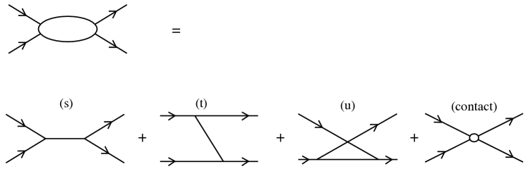
Figure 1: Decomposition of two-body interaction into s, t, u and c (contact) channels.

Microscopically, the pion couples to the constituent quarks that are dynamically generated by SSB. Combined with the quark model wave functions of hadrons, the coupling strengths as well as form factors are estimated, schematically by

$$V_{\pi hh^{\prime}}=\sum_{i}\langle h^{\prime}|V_{\pi q_{i}q_{i}}|h\rangle\,,$$ (1)

where the sum is taken over the light quarks ($i$) in the hadrons as shown in figure 2. This method works qualitatively well for nuclear interactions and is now extended to other hadrons for the study of hadronic molecules. Other meson interactions such as $\sigma$, $\omega$ and $\rho$ mesons are also employed but then more parameters are needed. In fact, the masses of these mesons are of the same order of the inverse of hadron size, and their contributions may be masked by the form factors. Thus, the pion interaction is the best known and under control. In most part of this paper, we test models of hadronic molecules with the pion interaction.

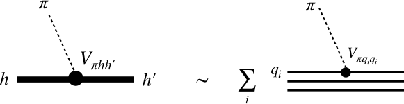
Figure 2: Schematic view of a pion hadron (nucleon in this figure) coupling.

Another feature of the pion interaction is in its tensor structure. This is the consequence of SSB of chiral symmetry which leads to pseudoscalar nature of the pion with spin-parity $J^{P}=0^{-}$. Therefore, the coupling structure of the pion to hadrons is of $\boldsymbol{\sigma}\cdot\bi r$ type. This leads to the tensor force causing mixing of orbital motions of different angular momenta by two units. This provides extra attraction which contributes significantly to the formation of molecules. Although the importance of the tensor force has long been recognized in nuclear physics [27, 28], quantitative understanding has progressed by developments in the microscopic treatment of many-body systems and in computer power [29, 30, 31, 32].

In addition to the pion exchange interaction at long distances, we also discuss $s$-channel interactions at short distances where the incoming hadrons merge into a single hadron (one-particle) as an intermediate state (see figure 1). Hence this process leads to the mixing of configurations, an extended molecular structure of two particles and a compact one-particle state. The problem is also related to the question of the so-called compositeness [33, 34, 35, 36, 37]. We emphasize the importance of such mixing for $X(3872)$; a molecular component of $D\bar{D}^{*}$ at long distances and a $c\bar{c}$ component at short distances [38].

1.4 Contents of this paper

This paper is organized as follows. In section 2, we show how the Yukawa vertex of a pion to heavy hadrons are derived. Coupling constants in different schemes are discussed in some detail. Estimation in the quark model is also discussed. In section 3, OPEP is derived with emphasis on general features of the potential. Special attention is paid to the tensor structure and form factors. A non-static feature is also discussed when the mass of the interacting hadrons changes, which is taken into account by an effective mass of the pion. In section 4, we discuss the structure of $X(3872)$. After briefly reviewing experimental status, we discuss the molecular nature made by the one-pion exchange. An important role of the short distance dynamics is also discussed, and consider a mixing structure of hadronic molecule coupled by a compact quark $c\bar{c}$ component. In section 5, a brief review for $Z_{c}$ with some discussions are given. Section 6 is for a few subjects for pentaquarks, where we quickly overview for a few candidates including the most recent ones from LHCb, $P_{c}$ baryons. We summarize the paper with some remarks and prospects in section 7.

2 Heavy hadron interactions

Hadronic molecules are composite systems of hadrons which are loosely bound or resonate. “Loosely” means that the binding or resonant energies are small as compared to the QCD scale of $\Lambda_{QCD}\sim$ some hundreds MeV, which is relevant to intrinsic structure of hadrons by quarks. In such a situation, the constituent hadrons can retain their intrinsic structure in the molecules. The interaction among the hadrons is colorless and its dominant part is expected to be dictated by meson exchanges. Among them, pion exchange interaction is the best under control. The pion couples to the light $u,d$ quarks, and their dynamics is determined by the nature of Nambu-Goldstone bosons of spontaneous breaking of chiral symmetry. This is the case if hadrons contain light $u,d$ quarks as constituents such as protons, neutrons and also heavy open flavor hadrons such as $D$ mesons ($c\bar{u}$) and $\Sigma_{c}$ baryons ($cuu$).

In this section, we discuss basic interactions of heavy mesons, that is the Yukawa vertices for $P$ and $P^{*}$ with the pion, where $P$ stands for $D$ or $\bar{B}$ meson, and $P^{*}$ for $D^{*}$ or $\bar{B}^{*}$. We also employ the notation $P^{(*)}$ for either $P$ or $P^{*}$. In addition to chiral symmetry features associated with light quarks, heavy quark spin symmetry also applies in the presence of heavy quarks (either charm $c$ or bottom $b$ quark) [39, 40]. In particular, heavy quark spin symmetry relates the mesons with different spins under spin transformations. For example, $P$-meson of spin-parity $J^{P}=0^{-}$ is a spin partner of $P^{*}$ meson of $J^{P}=1^{-}$; they are the same particles under heavy quark spin symmetry.

To implement the aspects of heavy quark spin and chiral symmetries in the effective Lagrangian, we shall quickly overview several issues such as a convention for heavy quark normalization, representations of heavy fields for $D$ and $D^{*}$ mesons, and their properties under the heavy quark spin and chiral symmetry transformations. We also discuss how the relevant coupling constants are determined. We see that the constituent picture of the light quark coupled by the pion consistently describes the decay properties of the $D^{(*)}$ mesons as well as axial properties of the nucleon.

2.1 Heavy fields

When considering quantum fields of heavy particles of mass $m_{H}$, it is convenient to redefine the effective heavy fields in which the rapidly oscillating component in time, $\exp(-im_{H}t)$, is factored out. For QCD “heavy” means that $m_{H}$ is sufficiently larger than the QCD scale, $\Lambda_{\rm QCD}\ll m_{H}$, and the heavy quarks almost stay on mass-shell with quantum fluctuations being suppressed. In accordance with the redefinition of the field, the normalization of the effective heavy fields are naturally modified from the familiar one of quantum fields by the factor $\sqrt{m_{H}}$.

To show this point let us consider the standard Lagrangian for a complex scalar meson field of heavy mass $m_{H}$, $\phi(x)=\frac{1}{\sqrt{2}}(\phi_{1}(x)+i\phi_{2}(x))$,

$${{{\cal L}}}=(\partial_{\mu}\phi^{\dagger})(\partial^{\mu}\phi)-m_{H}^{2}\phi^{\dagger}\phi\,.$$ (2)

The factor 1/2 is recovered when using the real components $\phi_{1,2}$. From this Lagrangian, the current is given by

$$j^{\mu}=i\left(\phi^{\dagger}\partial^{\mu}\phi-\phi\partial^{\mu}\phi^{\dagger}\right)\,.$$ (3)

The field expansion may be done as

$$\phi(x) = \int\frac{\rmd^{3}p}{2E(2\pi)^{3}}\left(e^{-ipx}a_{\bi p}+e^{+ipx}b_{\bi p}^{\dagger}\right),\;\;\;E=\sqrt{m_{H}^{2}+\bi p^{2}}$$ (4)

in the standard conventions.

In the heavy mass limit $m_{H}\to\infty$, the particle is almost on-mass shell, and it is convenient to define the velocity $v_{\mu},v^{2}=1$ which defines the on-shell momentum $m_{H}v_{\mu}$. Thus the momentum fluctuation $k_{\mu}$ around it is considered to be small, $k_{\mu}\ll m_{H}$

$$p_{\mu}=m_{H}v_{\mu}+k_{\mu}\,.$$ (5)

Moreover the Hilbert space of different heavy particle numbers decouple because particle-antiparticle creation is suppressed in the considering energy scale.

Hence we define the heavy field by

$$\phi(x)=\exp(-im_{H}vx)\tilde{\phi}(x)\,.$$ (6)

This means that the energy of $\tilde{\phi}(x)$ is measured from $m_{H}$. Inserting the relation

$$\partial_{\mu}\phi(x)=(-im_{H}v_{\mu}\tilde{\phi}(x)+\partial_{\mu}\tilde{\phi}(x))\exp(-im_{H}vx)$$ (7)

into (2), we find

$${{{\cal L}}}=2im_{H}(\tilde{\phi}^{\dagger}v\partial\tilde{\phi})+{\cal O}(1)$$ (8)

and for the current,

$$j^{\mu}=2m_{H}\tilde{\phi}^{\dagger}v^{\mu}\tilde{\phi}+{\cal O}(1)\,,$$ (9)

where in both equations we have only shown the leading term of order ${\cal O}(m_{H})$. Note that the mass term in (2) disappears in the Lagrangian as expected because the energy is measured from $m_{H}$. By absorbing the factor $m_{H}$ into the field as

$$\phi_{H}\equiv\sqrt{m_{H}}\tilde{\phi}$$ (10)

then we have

$${{{\cal L}}}_{H} = 2i(\phi_{H}^{\dagger}v\partial\phi_{H})\,,$$

$$j_{H}^{\mu} = 2\phi_{H}^{\dagger}v^{\mu}\phi_{H}\,.$$ (11)

In this convention, the heavy (boson) field $\phi_{H}$ carries dimension 3/2 in units of mass, unlike 1 in the standard boson theory. In this paper, as in many references, we follow this convention, while we also come back to the ordinary convention of dimension 1. In terms of one-particle states, these two conventions correspond to different normalizations [40]

$$\langle v|v\rangle=\sqrt{2v_{0}}\ ,\;\;\;\langle p|p\rangle=\sqrt{2p_{0}}\ ,\;(p_{0}=E)\ .$$ (12)

Moreover the one-particle to vacuum matrix element of the field is given by

$$\langle 0|\phi_{H}(x)|p\rangle=\sqrt{m_{H}}e^{-ipx}\ .$$ (13)

2.2 Interaction Lagrangian

Let us consider the pseudoscalar $P$ and vector $P^{*}$ mesons as a pair of heavy quark $Q$ and light antiquark $\bar{q}$ in the lowest S-wave orbit. Having overviewed the features of heavy particles in the previous subsection, the heavy meson field is defined in the frame of a fixed velocity $v_{\mu}$ and contains multiplet of spin 0 pseudoscalar and spin 1 vector mesons. They are $(D,D^{*})$ in the charm sector, and $(\bar{B},\bar{B}^{*})$ for the bottom sector. For convenience, namings and quark contents of various mesons are given in table 2. In this article throughout, we place symbols without bar on the left of those with bar. This is a convention that is consistent with quark model calculations.

Table 2: Various heavy mesons and quark contents, where $q=u,d$ quarks.

Mesons $P^{(*)}$	$K^{(*)}$	$\bar{K}^{(*)}$	$D^{(*)}$	$\bar{D}^{(*)}$	$B^{(*)}$	$\bar{B}^{(*)}$
Quark contents	$q\bar{s}$	$s\bar{q}$	$c\bar{q}$	$q\bar{c}$	$q\bar{b}$	$b\bar{q}$

A convenient way to express such heavy meson fields (including antiparticles) is

$$H^{a} = \frac{1+{v/}}{2}\left[-P^{*a}_{\mu}\gamma^{\mu}+P^{a}\gamma_{5}\right]\sim Q\bar{q}\ ,$$

$$\bar{H}^{a} = \gamma_{0}H^{\dagger}_{a}\gamma_{0}=\left[-(P^{*\dagger})^{a}_{\mu}\gamma^{\mu}-(P^{\dagger})^{a}\gamma_{5}\right]\frac{1+{v/}}{2}\sim q\bar{Q}\ ,$$ (14)

where $P^{a}$ and $P^{*a}_{\mu}$ carry an index of isospin 1/2, $a=1,2\sim u,d$. The factor $(1+{v/})/{2}$ is a projector to constrain the heavy quark velocity at $v$. We employ the convention for $\gamma$-matrices

$$\gamma^{0}=\left(\begin{array}[]{c c}1&0\\ 0&-1\end{array}\right)\,,\;\;\;\gamma^{i}=\left(\begin{array}[]{c c}0&\sigma_{i}\\ -\sigma_{i}&0\end{array}\right)\,,\;\;\;\gamma_{5}=\left(\begin{array}[]{c c}0&1\\ 1&0\end{array}\right)\,,$$ (21)

and contractions $A^{\mu}B_{\mu}=A^{0}B_{0}+A^{i}B_{i}=A^{0}B_{0}-\bi A\cdot\bi B$. For later convenience, we express the meson fields explicitly in terms of the quark fields

$$P^{a}=\bar{q}^{a}i\gamma_{5}Q,\;\;\;P^{*a}_{\mu}=\bar{q}^{a}\gamma_{\mu}Q\ .$$ (22)

Let us consider $D^{+}=\bar{d}i\gamma_{5}c,D^{*+}_{\mu}=\bar{d}\gamma_{\mu}c$, where $d,c$ express the Dirac fields for the down and charm quarks. Under charge conjugation transformations,

$$c\to-i(\bar{c}\gamma^{0}\gamma^{2})^{T},\;\;\;\bar{d}\to-i(\gamma^{0}\gamma^{2}d)^{T}\ ,$$ (23)

we can verify that

$$D^{+}\to D^{-}=(D^{+})^{\dagger},\;\;\;D^{*+}_{\mu}\to-D^{*-}_{\mu}=-(D^{*+}_{\mu})^{\dagger}\ .$$ (24)

In this convention, again using the notation $P$’s, the operators for the charge conjugated anti-particles are $P^{\dagger}$ for pseudoscalars and $-P^{*\dagger}_{\mu}$ for vectors. The corresponding states are defined by

$$|P\rangle=P^{\dagger}|0\rangle,\;\;\;|P^{*}_{\mu}\rangle=P^{*\dagger}_{\mu}|0\rangle\ ,$$

$$|\bar{P}\rangle=P|0\rangle,\;\;\;|\bar{P}^{*}_{\mu}\rangle=-P^{*}_{\mu}|0\rangle\ .$$ (25)

These relations will be used when forming eigenstates of charge conjugation of molecules formed by $P^{(*)}$ and $\bar{P}^{(*)}$ mesons.

The spin multiplet nature of $P$ and $P^{*}$ is verified by writing (14) in the rest frame $v^{\mu}=(1,0,0,0)$, where only the spatial components remain for the vector meson as its degrees of freedom

$$H=\left(\begin{array}[]{ c c}0&P+{\boldsymbol{\sigma}}\cdot\bi{P}^{*}\\ 0&0\end{array}\right)\ .$$ (28)

Here the isospin label $a$ is suppressed, since it is irrelevant under spin transformations. The combination $P+\bi{\boldsymbol{\sigma}}\cdot\bi{P}^{*}$ indicates that $P$ and $\bi P^{*}$ are the spin multiplet of $(1/2,1/2)$ representation of the heavy and light spin group $SU(2)_{Q}\times SU(2)_{q}$. They transform under the heavy and light spin transformations as

$$H\to\exp(i\bi{\boldsymbol{\Sigma}}\cdot\bi\boldsymbol{\theta}_{Q})H\exp(-i\bi{\boldsymbol{\Sigma}}\cdot\bi\boldsymbol{\theta}_{q})\ ,$$ (29)

where $\bi{\boldsymbol{\Sigma}}$ are the four component spin matrices defined by $\Sigma_{k}=\frac{i}{2}\epsilon_{ijk}[\gamma^{i},\gamma^{j}]$, and $\bi\boldsymbol{\theta}_{Q}$ and $\bi\boldsymbol{\theta}_{q}$ are the rotation angles of heavy and light quark spins, respectively. The diagonal part of $\bi\boldsymbol{\theta}_{Q}=\bi\boldsymbol{\theta}_{q}$ corresponds to the total spin rotation.

Chiral symmetry property of the heavy meson field (14) is inferred by the constituent nature of the light quark $q$. It is subject to nonlinear transformations of chiral symmetry [41, 42, 43, 44]. In this article, we consider two light flavors and therefore $SU(2)_{L}\times SU(2)_{R}$ is the relevant chiral symmetry group, where the left ($L$) and right ($R$) transformations act on the two isospin groups. Explicitly, the quark field $q$ of isospin 1/2 are transformed as

$$q\to h(g_{R},g_{L},\boldsymbol{\pi}(x))q\ ,$$ (30)

where the isospin $SU(2)$ matrix function $h(g_{R},g_{L},\boldsymbol{\pi}(x))$ characterizes nonlinear chiral transformations determined by global chiral transformations of $g_{L,R}\in SU(2)_{L,R}$ at the pion field $\boldsymbol{\pi}(x)$. Therefore, the heavy meson fields of isospinor transforms under chiral symmetry transformations as

$$H\to Hh^{\dagger},\;\;\;\bar{H}\to h\bar{H}\ .$$ (31)

The isovector pion field parametrizes unitary matrices as

$$U(x)=\exp\left(i\frac{\boldsymbol{\tau}\cdot\boldsymbol{\pi}(x)}{f_{\pi}}\right)\ ,$$ (32)

which linearly transforms as

$$U(x)\to g_{L}U(x)g_{R}^{\dagger}\ .$$ (33)

The nonlinear transformation for the pion field is then conveniently expressed in terms of the square root

$$\xi(x)=\exp\left(i\frac{\boldsymbol{\tau}\cdot\boldsymbol{\pi}(x)}{2f_{\pi}}\right)\ ,$$ (34)

which is subject to

$$\xi\to h\xi g_{R}^{\dagger}=g_{L}\xi h^{\dagger}\ .$$ (35)

Here $f_{\pi}$ is the pion decay constant for which our convention is $f_{\pi}\sim 93$ MeV. The $\xi$-field defines the vector and axial-vector currents

$$V_{\mu} = \frac{1}{2}(\xi^{\dagger}\partial_{\mu}\xi+\xi\partial_{\mu}\xi^{\dagger})\ ,$$

$$A_{\mu} = \frac{1}{2}(\xi^{\dagger}\partial_{\mu}\xi-\xi\partial_{\mu}\xi^{\dagger})\ ,$$ (36)

which are transformed as

$$V_{\mu} \to h(V_{\mu}+\partial_{\mu})h^{\dagger}\ ,$$

$$A_{\mu} \to hA_{\mu}h^{\dagger}\ .$$ (37)

Note that the currents (36) are anti-Hermitian. Moreover, the vector and axial-vector currents are of even and odd power with respect to the pion field (see (39)), while properly satisfying the parity of the currents, $1^{-}$ and $1^{+}$, respectively.

With the heavy quark spin and chiral transformation properties established, we can write down the invariant Lagrangian. To the leading order of derivative expansion, we find

$${{{\cal L}}} = -i\tr\left[Hv_{\mu}(\partial^{\mu}+iV^{\mu})\bar{H}\right]+ig_{A}\tr\left[H\gamma_{\mu}\gamma_{5}A^{\mu}\bar{H}\right]\ .$$ (38)

By expanding the vector and axial-vector currents, $V_{\mu}$ and $A_{\mu}$ with respect to the pion field,

$$V_{\mu} = \frac{i}{4f_{\pi}^{2}}\boldsymbol{\tau}\cdot\boldsymbol{\pi}\times\partial_{\mu}\boldsymbol{\pi}+\cdots$$

$$A_{\mu} = \frac{i}{2f_{\pi}}\boldsymbol{\tau}\cdot\partial_{\mu}\boldsymbol{\pi}+\cdots$$ (39)

the vector current leads to the pion-hadron interaction of the so-called Weinberg-Tomozawa interaction, while the axial vector current to the Yukawa coupling. The former strength is determined by the pion decay constant while the latter contains one unfixed parameter, the axial coupling constant $g_{A}$. In the present scheme it corresponds to the one of the constituent quark as discussed in section 2.5. By inserting the expansion (39), we find the $PP^{*}\pi$ and $P^{*}P^{*}\pi$ interaction Lagrangians

$${{{\cal L}}}_{P^{*}P\pi} = -\frac{g_{A}}{f_{\pi}}\left(P_{\mu}^{*a}\partial^{\mu}({\boldsymbol{\tau}\cdot\boldsymbol{\pi}})_{ab}(P^{\dagger})^{b}+P^{a}\partial^{\mu}({\boldsymbol{\tau}\cdot\boldsymbol{\pi}})_{ab}(P^{*\dagger}_{\mu})^{b}\right)\ ,$$

$${{{\cal L}}}_{P^{*}P^{*}\pi} = -i\frac{g_{A}}{f_{\pi}}\epsilon^{\alpha\beta\gamma\delta}v_{\alpha}P_{\beta}^{*a}\partial_{\gamma}(\boldsymbol{\tau}\cdot\boldsymbol{\pi})_{ab}(P^{*\dagger})^{b}_{\delta}\ .$$ (40)

As anticipated, the strengths of these interactions are given by one coupling constant $g_{A}$, which is a consequence of heavy quark spin symmetry.

2.3 Meson decays I, $D^{*}\to D\pi$

To see the use of (40) together with the heavy quark normalization, let us consider the simplest and important example of meson decays, $D^{*+}(\lambda,p)\to D^{+}(p^{\prime})\pi^{0}(q)$, where $\lambda$ labels the polarization of $D^{*+}$. The relevant matrix element for these charged states is ($P\sim D$)

$$\langle P(p^{\prime})\pi(q)|{{\cal L}}_{P^{*}P\pi}|P^{*}(\lambda,p)\rangle=-m_{H}\frac{ig_{A}}{f_{\pi}}q_{\nu}\epsilon^{\nu}(\lambda)e^{i(-p+q+p^{\prime})x}\equiv Ve^{i(-p+q+p^{\prime})x}\ ,$$ (41)

where $\epsilon^{\nu}(\lambda)$ is the polarization vector of the $D^{*}$ meson, and we have used the relation for the matrix elements;

$$\langle P(p^{\prime})|P(x)|0\rangle = \sqrt{m_{H}}e^{+ip^{\prime}x},$$

$$\langle 0|P^{*}_{\mu}(x)|P^{*}(\lambda,p)\rangle = \sqrt{m_{H}}\epsilon_{\mu}(\lambda)e^{-ipx},$$

$$\langle\pi(q)|\pi(x)|0\rangle = e^{+iqx}\ .$$ (42)

Here the masses of $D$ and $D^{*}$ mesons are regarded sufficiently heavy and set equal to $m_{H}$. For later convenience, we summarize the other matrix elements which are needed for the computations of the transition amplitudes $PP^{*}\to P^{*}P$ and $\bar{P}\bar{P}^{*}\to\bar{P}^{*}\bar{P}$ in table 3. By using the relations of (25), one can verify these relative signs.

Table 3: Relative signs of various $P^{(*)}P^{(*)}\pi$ couplings including antiparticles.

$\langle P\pi|{{{\cal L}}}|P^{*}\rangle$	$\langle P^{*}\pi|{{{\cal L}}}|P\rangle$	$\langle\bar{P}^{*}\pi|{{{\cal L}}}|\bar{P}\rangle$	$\langle\bar{P}\pi|{{{\cal L}}}|\bar{P}^{*}\rangle$
+	$-$	+	$-$

Now the decay width is computed by

$$\Gamma=\frac{1}{2m_{D^{*}}}\int\frac{\rmd^{3}p^{\prime}}{2E_{D}(\bi p^{\prime})(2\pi)^{3}}\frac{\rmd^{3}q}{2E_{\pi}(\bi q)(2\pi)^{3}}(2\pi)^{4}\delta^{4}(p-p^{\prime}-q)|V|^{2}\ .$$ (43)

Note that in the heavy mass limit, $m_{D^{*}}\sim E_{D}\sim m_{H}$, heavy meson mass $m_{H}$ dependence in $E_{D}(\bi p^{\prime})$ in the denominator and that in $|V|^{2}$ in the numerator cancel. The heavy mass independence is reasonable because the decay $D^{*+}\to D^{+}\pi^{0}$ occurs through the spin flip of the light quark which should not depend on the heavy mass of the spectator heavy quark. Fixing the polarization $\epsilon(\lambda)^{\nu}$ of initial $D^{*}$ meson and performing the phase space integral

$$\int\frac{\rmd^{3}p^{\prime}}{2E_{P}(\bi p^{\prime})(2\pi)^{3}}\frac{\rmd^{3}q}{2E_{\pi}(\bi q)(2\pi)^{3}}(2\pi)^{4}\delta^{4}(P_{f}-P_{i})=\frac{q}{16\pi^{2}(E_{D}+E_{\pi})}\int d\Omega$$ (44)

together with the angle average of $|q_{\nu}\epsilon^{\nu}|^{2}\to|\bi q\cdot\bi\epsilon|^{2}\to q^{2}/3$, we find

$$\Gamma_{D^{*+}\to D^{+}\pi^{0}}=\frac{q^{3}}{24\pi}\left(\frac{m_{H}}{m_{D}^{*}}\right)^{2}\left(\frac{g_{A}}{f_{\pi}}\right)^{2}\to\frac{q^{3}}{24\pi}\left(\frac{g_{A}}{f_{\pi}}\right)^{2}\ .$$ (45)

Using the experimental data

$$\Gamma_{D^{*+}\to D^{+}\pi^{0}} = 83.4\;{\rm keV}\times 30.7\;\%\ ,$$

$$m_{D^{*+}} = 2010\;{\rm MeV},\;\;m_{D^{+}}=1870\;{\rm MeV},\;\;m_{\pi^{0}}=135\;{\rm MeV},$$

$$q = 38\;{\rm MeV},\;\;f_{\pi}=93\;{\rm MeV},$$ (46)

we find

$$g_{A}\sim 0.55\ .$$ (47)

This value is obtained in the limit $m_{D},m_{D^{*}}\to\infty$ using the formula (45). If we take into account their finite values, we find $g_{A}\sim 0.53$. This estimates uncertainties of few percent at minimum in the discussions based on the leading terms of the heavy quark symmetry.

2.4 Meson decays II, $K^{*}\to K\pi$

Now it is instructive to demonstrate another textbook like calculation for the decay $K^{*}\to K\pi$, which is the analog of $D^{*}\to D\pi$ by replacing the charm quark by the (anti)strange quark. A commonly used Lagrangian in a flavor SU(3) symmetric form is written as

$${{\cal L}}_{K^{*}K\pi} = -igK^{\dagger}\partial^{\mu}(\boldsymbol{\tau}\cdot\boldsymbol{\pi})K^{*}_{\mu}+(h.c.)$$ (48)

$$= -ig(K^{-}\partial^{\mu}\pi^{0}+\sqrt{2}\bar{K}^{0}\partial_{\mu}\pi^{-})K^{*+}_{\mu}+\cdots\ .$$

where $g$ is the coupling constant of a vector meson with two pseudoscalar mesons. In the SU(3) limit it is the $\rho\to\pi\pi$ coupling constant and is given to be $g\sim 6$ [44, 45, 46]. In this convention, the normalization is

$$\langle 0|K^{(*)}(x)|K^{(*)}(p)\rangle=e^{-ipx}\ ,$$ (49)

such that there are $2E$ particles in a unit volume. The matrix element of the above Lagrangian is then (again for the neutral pion decay)

$$\langle K^{+}(\bi q)\pi^{0}(-\bi q)|{\cal L}_{K^{*}K\pi}|K^{*+}({\rm at}\;{\rm rest})\rangle=-igq_{\mu}\epsilon^{\mu}\ .$$ (50)

Therefore, we find the formula

$$\Gamma_{K^{*+}\to K^{+}\pi^{0}}=\frac{q^{3}}{24\pi m_{K^{*}}(E_{K}+E_{\pi})}g^{2}\ .$$ (51)

Here if we break $SU(3)$ symmetry and take heavy mass limit for the strange quark, $m_{K^{*}}\sim E_{K}\to m_{H}$, we find the total decay width

$$\Gamma_{tot}=\frac{q^{3}}{8\pi}\left(\frac{g}{m_{H}}\right)^{2}\ .$$ (52)

By using the experimental data

$$\Gamma_{K^{*+}\to K^{+}\pi^{0}}=50\times\frac{1}{3}\;{\rm MeV},\;\;\;m_{K^{*}}=890\;{\rm MeV},\;\;\;q=290\;{\rm MeV}\ ,$$ (53)

we find

$$g\sim 6.4\ ,$$ (54)

which is close to the coupling constant of the $\rho$ meson decay, $g(\rho\to\pi\pi)\sim 6$.

Comparing equations (45) and (52) we find

$$\frac{g_{A}}{f_{\pi}}=\frac{g}{m_{H}}\,.$$ (55)

This is nothing but the generalized Goldberger-Treiman relation, implying that the coupling constant $g$ scales as the meson mass $m_{H}$, when $g_{A}$ is independent of $m_{H}$ as we shall discuss in the next subsection. In other words, flavor symmetry breaking for the coupling constant $g$ defined by the Lagrangian (48) scales as that of the corresponding meson masses. As a matter of fact, the coupling constant $g$ for the decay of $D^{*}$ is estimated to be $g\sim 12$, which is different from $g\sim 6$ estimated from the decay of $K^{*}$ by about factor two. This difference is explained by the difference in the masses of $D^{*}$ and $K^{*}$ mesons, $m_{D^{*}}\sim 2000$ and $m_{K^{*}}\sim 890$ MeV within about 10 % accuracy.

2.5 Quark model estimate

In this subsection we show that the coupling constant $g_{A}$ in the Lagrangian (40) is nothing but the quark axial-vector coupling constant in the non-relativistic quark model. Let us start with the $\pi qq$ Lagrangian in the axial vector type

$${\cal L}_{\pi qq}=\frac{g_{A}^{q}}{2f_{\pi}}\bar{q}\gamma_{\mu}\gamma_{5}\partial^{\mu}\pi q\ ,$$ (56)

where we have denoted the quark axial-vector coupling by $g_{A}^{q}$, and ignored isospin structure for simplicity. This Lagrangian operates to the light quark-pion vertex at position $\bi x_{1}$ as shown in figure 3, where assignments of various variables are also shown. For example, the the center of mass and relative coordinates are defined by

$$\bi X=\frac{m\bi x_{1}+M\bi x_{2}}{m+M}\,,\;\;\;\bi r=\bi x_{1}-\bi x_{2}\ ,$$ (57)

with $m,M$ being the masses of the light and heavy quarks,

In the non-relativistic limit, the matrix element of (56) for $\bar{D}^{*}$(at rest) $\to\bar{D}(-\bi q)\pi(+\bi q)$ is given as [47]

$${\cal L}_{\pi qq}\to i\frac{g_{A}^{q}}{2f_{\pi}}\chi_{f}^{\dagger}\left[\frac{\omega_{\pi}}{m}\boldsymbol{\sigma}\cdot\bi p_{i}-\left(1+\frac{\omega_{\pi}}{2m}\right)\boldsymbol{\sigma}\cdot\bi q\right]\chi_{i}e^{+i\omega_{\pi}t-i\bi q\cdot\bi x_{1}}\ ,$$ (58)

where $\chi_{i,f}$ are the quark wave functions of the initial $D^{*}$ and final $D$ meson, $(\omega_{\pi},\bi q)$ the energy and momentum of the pion, $\bi p_{i}$ the momentum of the quark in the initial $\bar{D}^{*}$ meson. For a notational reason in the definition of the quark model wave function as explained below, here we consider the decay of $\bar{D}^{*}$ rather than $D^{*}$.

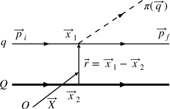
Figure 3: Quark model diagram for the decay of $D^{*}\to D\pi$.

The wave functions $\chi_{i,f}$ are written as a product of the plain wave for the center of mass and internal part including spin, $\phi_{i,f}(\bi r)$

$$\chi_{i,f}(t,\bi X,\bi r)=\exp\left(-i\omega_{i,f}t+i\bi P_{i,f}\cdot\bi X\right)\phi_{i,f}(\bi r)\ ,$$ (59)

where $\omega_{i,f}$ are the energies of the initial $\bar{D}^{*}$ and final $\bar{D}$ mesons. Expressing $\bi p_{i}$ by the relative momentum $\bi p_{r}$ as

$$\bi p_{i}=\frac{m}{m+M}\bi P_{i}+\bi p_{r}\ ,$$ (60)

we can perform the $t$ and $\bi X$-integral leading to the total energy-momentum conservation, leaving the $\bi r$ integral as

$$\frac{ig_{A}^{q}}{2f_{\pi}}\int\rmd^{3}r\ \phi_{f}^{\dagger}(\bi r)\left[\frac{\omega_{\pi}}{m}\left(\frac{m}{m+M}\boldsymbol{\sigma}\cdot\bi P_{i}-i\boldsymbol{\sigma}\cdot{\bi\nabla}_{r}\right)\left(1+\frac{\omega_{\pi}}{2m}\right)\boldsymbol{\sigma}\cdot\bi q\right]\phi_{i}(\bi r)e^{-i\tilde{\bi q}\cdot\bi r}\ ,$$ (61)

where effective momentum transfer is defined by

$$\tilde{\bi q}=\frac{M}{m+M}\bi q\ ,$$ (62)

and the relative momentum $\bi p_{r}$ is replaced by ${-i\bi\nabla}_{r}$. Using the harmonic oscillator wave function for both $\phi_{i}$ and $\phi_{f}$,

$$\phi(\bi r)=\frac{1}{\sqrt{4\pi}}\frac{2\alpha^{3/2}}{\pi^{1/4}}\exp\left(-\frac{\alpha^{2}}{2}r^{2}\right)\ ,$$ (63)

with the size parameter $\alpha$, after some computation, we find

$$\langle D\pi|{\cal L}_{\pi qq}|D^{*}\rangle = \frac{ig_{A}^{q}}{2f_{\pi}}\left(1+\frac{\omega_{\pi}}{2m}\left(-1+\frac{M}{m+M}\right)\right)|\bi q|\langle\boldsymbol{\sigma}\cdot\hat{\bi}q\rangle F(\bi q^{2})\ ,$$ (64)

$$F(\bi q^{2}) = \int\rmd^{3}r\ \phi_{f}^{\dagger}(\bi r)\phi_{i}(\bi r)e^{i\bi q\cdot\bi r}\ .$$ (65)

For small $|\bi q|$, we set the form factor $F(\bi q^{2})\to 1$. For the spin matrix element $\langle\boldsymbol{\sigma}\cdot\hat{\bi}q\rangle$, we evaluate the transition

$$D^{*}(S=1,S_{z}=1)\to D(S=S_{z}=0),\;\;\hat{\bi}q\sim\hat{\bi}z\ .I$$ (66)

Having the spin wave functions

$$|S=1,S_{z}=0\rangle=\frac{1}{\sqrt{2}}(\uparrow\downarrow+\downarrow\uparrow)\,,\;\;\;|S=S_{z}=0\rangle=\frac{1}{\sqrt{2}}(\uparrow\downarrow-\downarrow\uparrow)\ ,$$ (67)

and with the understanding that the spin operator acts on the first (left) spin state for the light quark, we find $\langle S=0|\boldsymbol{\sigma}\cdot\hat{\bi}q|S=1\rangle=1\ .$

These results are compared with the matrix element (41), where we may set $q^{\mu}=(0,0,0,|\bi q|)$ and $q^{\mu}\epsilon_{\mu}=-|\bi q|$. Suppressing the second term in the heavy quark limit $M\to\infty$, we find the relation

$$g_{A}=g_{A}^{q}$$ (68)

in the limit $|\bi q|\to 0$.

Usually in the quark model $g_{A}$ is assumed to be unity, $g_{A}^{q}=1$. However, it is known that this overestimates the axial couplings of various hadrons. For the nucleon it is known that the quark model predicts $g_{A}^{N}=5/3$ [44]. In the quark model, the nucleon $g_{A}$ is defined to be the matrix element of spin and isospin operator

$$\sum_{n=1,2,3}\sigma_{i}(n)\tau^{a}(n)\ .$$ (69)

Therefore, effectively the reduction of $g_{A}^{q}\sim 0.7$ is needed to reproduce the data. Similarly heavy baryon transitions such as $\Sigma_{c}^{(*)}\to\Lambda_{c}$ consistently implies small $g_{A}^{q}$ [47]. How baryon $g_{A}$ is computed is found in Refs. [44, 47].

3 Meson exchange potential

In this section, we derive meson exchange potentials for the study of hadronic molecules. Starting from the classic method for the derivation, we revisit the OPEP for the nucleon ($N$). We find it is useful to recognize important and universal features of meson exchange potentials.

3.1 Simple exercise

Let us illustrate a simple example for a scalar field $\phi$ interacting with the exchange of a scalar $\pi$ meson of mass $m$. The extension to the case of physical pion will be done later in a rather straightforward manner. The model Lagrangian is

$${\cal L}=\frac{1}{2}(\partial_{\mu}\pi)^{2}-\frac{m^{2}}{2}\pi^{2}-\frac{g}{2}\pi\phi^{2}+({\rm kinetic\ terms\ of\ }\phi)\ ,$$ (70)

from which the equation of motion and a special solution for $\pi$ are obtained as

$$(\partial^{2}+m^{2})\pi(x) = -\frac{g}{2}\phi(x)^{2}\ ,$$

$$\hskip 51.21495pt\pi(x) = -\frac{g}{2}\int\rmd^{3}y\ \langle x|\frac{1}{\partial^{2}+m^{2}}|y\rangle\phi(y)^{2}\ .$$ (71)

We note that in this example, the coupling constant $g$ carries dimension of unit mass.

The potential energy for $\phi$ is given by the energy shift $\Delta E$ due to the interaction;

$$\Delta E = +\frac{g}{2}\int\rmd^{3}x\ \pi(x)\phi^{2}(x)$$ (72)

$$= \left(\frac{g}{2}\right)^{2}\int\rmd^{3}x\rmd^{3}y\ \phi^{2}(x)\langle x|\frac{-1}{\partial^{2}+m^{2}}|y\rangle\phi(y)^{2}\ ,$$

where in the second line we have used the solution of (71). Inserting the complete set and representing the propagator in the momentum representation, $\int\rmd^{3}p/(2\pi)^{3}|\bi{p}\rangle\langle\bi{p}|$, we find the expression

$$\Delta E = \int\rmd^{3}x\rmd^{3}y\ \phi^{2}(\bi{x})\left[\int\frac{\rmd^{3}q}{(2\pi)^{3}}\frac{-g^{2}}{-p^{2}+m^{2}}e^{i\bi{q}\cdot(\bi{x}-\bi{y})}\right]\phi(\bi{y)}^{2}\ .$$ (73)

Now we regard $\phi$ as a field operator and expand in momentum space. Then consider a scattering process of $\bi p_{1},\bi p_{2}\to\bi p_{1}^{\prime},\bi p_{2}^{\prime}$ as shown in figure 4. Taking the matrix element $\langle\bi p_{1}^{\prime},\bi p_{2}^{\prime}|\Delta E|\bi p_{1},\bi p_{2}\rangle$ and performing $x,y$, and $q$ integrals, we find

$$\Delta E=(2\pi)^{3}\delta(\bi p_{1}+\bi p_{2}-\bi p_{1}^{\prime}-\bi p_{2}^{\prime})\frac{-g^{2}}{-q^{2}+m^{2}}\ .$$ (74)

Remarks are in order.

• The energy shift $\Delta E$ (73) is for the entire volume $V\sim(2\pi)^{3}\delta(\bi p_{1}+\bi p_{2}-\bi p_{1}^{\prime}-\bi p_{2}^{\prime})\to\delta^{3}(0)$, and also for the normalization of $2E$ $\phi$-particles per unit volume. In the center-of-mass frame, energies of the two particles are the same and conserved, $E=\sqrt{\bi p^{2}+M^{2}}$, where $M$ is the mass of $\phi$.

  Therefore, the energy shift per unit volume and per particle is given by

  $$\Delta E=\frac{1}{(2E)^{2}}\frac{-g^{2}}{-q^{2}+m^{2}}\ .$$ (75)

• In the non-relativistic limit for the $\phi$ particle, we can take the static limit where the energy transfer $q^{0}$ is neglected such that $-q^{2}\to+\bi{q}^{2}$, and $E\sim M$. This defines the potential in momentum space

  $$V(\bi{q})=-\frac{1}{(2M)^{2}}\frac{g^{2}}{\bi{q}^{2}+m^{2}}\ ,$$ (76)

  and in turn

  $$V(\bi{r})=\int\frac{\rmd^{3}q}{(2\pi)^{3}}\frac{1}{(2M)^{2}}\frac{-g^{2}}{\bi{q}^{2}+m^{2}}e^{i\bi{q}\cdot\bi{r}}=-4\pi\left(\frac{g}{2M}\right)^{2}\frac{e^{-mr}}{r}$$ (77)

  in coordinate space.

• Though obvious but not very often emphasized, the potential appears always attractive when the coupling square $g^{2}$ is positive. If the coupling structure has spin dependence this is no longer the case, otherwise always so. This is understood by the formula of second order perturbation theory where the intermediate state of $\phi\phi\pi$ in the pion-exchange process is in higher energy state than the initial $\phi\phi$ (see figure 4) . This fact is in contrast with what we know for the Coulomb force. The reason is that the latter is given by the unphysical component of the photon, which is manifest in the sign of the metric.

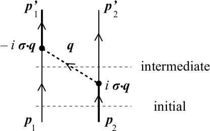
Figure 4: One meson exchange potential. The vertex structure of $\boldsymbol{\sigma}\cdot\bi q$ is needed for the one-pion exchange potential (OPEP) of the nucleon. For $\phi\phi$ or $NN$ the line widths of bold or normal are irrelevant. It will become relevant when discussing the potential for $P^{(*)}P^{(*)}$.

3.2 OPEP for the nucleon-nucleon $NN$

Now the most familiar and important example is the OPEP. In this section we will discuss OPEP for the nucleon, because the nucleon system is the best established, and can share common features with heavy hadrons. Since the pion is the pseudoscalar particle, the pion nucleon coupling is given either by the pseudoscalar or axial vector (pseudovector) form,

$${\cal L}_{\pi NN;PS} = -ig_{\pi NN}\bar{N}\gamma_{5}\boldsymbol{\tau}\cdot\boldsymbol{\pi}N\ ,$$

$${\cal L}_{\pi NN;PV} = -\frac{g_{A}^{N}}{2f_{\pi}}\bar{N}\gamma_{\mu}\gamma_{5}\boldsymbol{\tau}\cdot\partial^{\mu}\boldsymbol{\pi}N\ .$$ (78)

When the nucleons are on mass-shell, it is shown that the matrix elements for $N(\bi{p})\to N(\bi{p}^{\prime})\pi(\bi{q})$ in the two schemes are equivalent by using the equation of motion for the nucleon. The equivalence of the two expressions leads to the familiar Goldberger-Treiman relation

$$\frac{g_{\pi NN}}{m_{N}}=\frac{g_{A}^{N}}{f_{\pi}}\ .$$ (79)

In the non-relativistic limit, the equivalent matrix elements reduce to

$$\langle N(\bi{p}_{1}^{\prime})\pi^{a}(\bi{q})|{\cal L}_{\pi NN}|N(\bi{p}_{1})\rangle \to -i\frac{g_{A}^{N}}{2f_{\pi}}\boldsymbol{\sigma}_{1}\cdot\bi{q}\ \tau^{a}_{1}\ 2m_{N}\ ,$$

$$\langle N(\bi{p}_{2}^{\prime})|{\cal L}_{\pi NN}|N(\bi{p}_{2})\pi^{a}(\bi{q})\rangle \to +i\frac{g_{A}^{N}}{2f_{\pi}}\boldsymbol{\sigma}_{2}\cdot\bi{q}\ \tau^{a}_{2}\ 2m_{N}\ ,$$ (80)

where the two-component nucleon spinors are implicit and $a$ on $\pi$ and $\tau$-matrix is an isospin index. The extra factor $2m_{N}$ on the right-hand side appears due to the normalization of the nucleon (fermion) field when the state is normalized such that there are $2E\sim 2m_{N}$ nucleons in a unit volume. The positivity of the coupling square as discussed in the previous subsection is ensured by $\pm i$ in (80). Inserting these coupling structures into the general form of (76), we find the OPEP for the nucleon in the momentum space

$$V^{NN}_{\pi}(\bi{q})=-\left(\frac{g_{A}^{N}}{2f_{\pi}}\right)^{2}\frac{(\boldsymbol{\sigma}_{1}\cdot\bi{q}\,)(\boldsymbol{\sigma}_{2}\cdot\bi{q}\,)}{\bi{q}\,^{2}+m^{2}_{\pi}}\boldsymbol{\tau}_{1}\cdot\boldsymbol{\tau}_{2}\ .$$ (81)

Sometimes, this form is called the bare potential because the Lagrangian (78) does not consider the finite size structure of the nucleons and pions. The OPEP depends on $\bi{q}$, a feature consistent with the low energy theorems of chiral symmetry; interactions of the Nambu-Goldstone bosons contain their momenta. At low energies the $NN$ interaction (81) is of order ${\cal O}(\bi{q}^{2})$. In particular at zero momentum the interaction vanishes. In contrast, when $\bi{q}\to\infty$, the interaction approaches a constant. This requires a careful treatment for the large momentum or short range behavior of the interaction.

To see this point in more detail, let us decompose the spin factor $\boldsymbol{\sigma}_{1}\cdot\bi{q}\boldsymbol{\sigma}_{2}\cdot\bi{q}$ into the central and tensor parts

$$V^{NN}_{\pi}(\bi{q})=\left(\frac{g_{A}^{N}}{2f_{\pi}}\right)^{2}\frac{1}{3}\left[\left(-1+\frac{m^{2}_{\pi}}{\bi{q}\,^{2}+m^{2}_{\pi}}\right)\boldsymbol{\sigma}_{1}\cdot\boldsymbol{\sigma}_{2}+S_{12}(\hat{\bi q})\frac{-\bi{q}\,^{2}}{\bi{q}\,^{2}+m^{2}_{\pi}}\right]\boldsymbol{\tau}_{1}\cdot\boldsymbol{\tau}_{2}\ ,$$ (82)

where the tensor operator is defined by

$$S_{12}(\hat{\bi q})=3(\boldsymbol{\sigma}_{1}\cdot\hat{\bi q})(\boldsymbol{\sigma}_{2}\cdot\hat{\bi q})-\boldsymbol{\sigma}_{1}\cdot\boldsymbol{\sigma}_{2}\ .$$ (83)

The first term of (82) is the spin and isospin dependent central force, which has been further decomposed into the constant and the Yukawa terms. The constant term takes on the form of the $\delta$-function in the coordinate space. This singularity appears because the nucleon is treated as a point-like particle. In reality, nucleons have finite structure and the delta function is smeared out.

In the chiral perturbation scheme starting from the bare interaction of (81) the constant ($\delta$-function) term is kept and higher order terms are systematically computed by perturbation. In this case, low energy constants are introduced order by order together with a form factor with a cutoff to limit the work region of the perturbation series [48, 49]. To determine the parameters experimental data are needed. This is possible for the $NN$ force but not for hadrons in general. Alternatively, in nuclear physics the constant term is often subtracted. One of reasons is that the hard-core in the nuclear force suppresses the wave function at short distances and the $\delta$-function term is practically ineffective. Then form factors are introduced to incorporate the structure of the nucleon, and the cutoff parameters there are determined by experimental data.

In this paper, we employ the latter prescription, namely subtract the constant term and multiply the form factor. As in (82), the constant and Yukawa terms in the central force have opposite signs, and hence part of their strengths are canceled. The inclusion of the form factor in the Yukawa term is to weaken its strength, which is partially consistent with the role of the constant term. In practice, the central interaction of the OPEP is not very important for low energy properties. Rather the dominant role is played by the tensor force. We will see the important role of the tensor force in the subsequent sections.

So far we have discussed only the OPEP. In the so-called realistic nuclear force, to reproduce experimental data such as phase shifts and deuteron properties, more boson exchanges are included such as $\sigma$, $\rho$ and $\omega$ mesons [50, 51, 52]. Their masses are fixed at experimental data except for less established $\sigma$. Coupling constants and cutoff masses in the form factors are determined by experimental data of $NN$ phase shifts and deuteron properties. The resulting potentials work well for $NN$ scatterings up to several hundred MeV, and several angular momentum (higher partial waves). However, if we restrict discussions to low energy properties, which is the case for the present aim for exotic hadronic molecules, meson exchanges other than the pion exchange are effectively taken into account by the form factors. As discussed in the next section, we will see this for the deuteron.

Having said so much, let us summarize various formulae for the OPEP for $NN$. Subtracting the constant term with the form factor included we find

$$V^{NN}_{\pi}(\bi{q})\to\left(\frac{g_{A}^{N}}{2f_{\pi}}\right)^{2}\frac{1}{3}\left[\frac{m^{2}_{\pi}}{\bi{q}\,^{2}+m^{2}_{\pi}}\boldsymbol{\sigma}_{1}\cdot\boldsymbol{\sigma}_{2}+S_{12}(\hat{q})\frac{-\bi{q}\,^{2}}{\bi{q}\,^{2}+m^{2}_{\pi}}\right]F(\bi{q})\ \boldsymbol{\tau}_{1}\cdot\boldsymbol{\tau}_{2},$$ (84)

For the form factor we employ the one of dipole type

$$F(\bi{q})=\left(\frac{\Lambda^{2}-m_{\pi}^{2}}{\Lambda^{2}-q^{2}}\right)^{2}\to\left(\frac{\Lambda^{2}-m_{\pi}^{2}}{\Lambda^{2}+\bi{q}^{2}}\right)^{2}\ .$$ (85)

The potential in the $r$-space is obtained by performing the Fourier transformation as

$$V_{NN}^{\pi}(\bi r) = \int\frac{\rmd^{3}q}{(2\pi)^{3}}V(\bi{q})e^{i\bi{q}\cdot\bi{r}}$$ (86)

$$= \left(\frac{g_{A}^{N}}{2f_{\pi}}\right)^{2}\frac{1}{3}\left[\boldsymbol{\sigma}_{1}\cdot\boldsymbol{\sigma}_{2}C(r;m_{\pi},\Lambda)+S_{12}(\hat{r})T(r;m_{\pi},\Lambda)\right]\boldsymbol{\tau}_{1}\cdot\boldsymbol{\tau}_{2}\ .$$

where $C(r;m,\Lambda)$ and $T(r;m,\Lambda)$ are given by by

$$C(r;m,\Lambda) = \frac{m^{2}}{4\pi}\left[\frac{e^{-mr}}{r}-\frac{e^{-\Lambda r}}{r}-\frac{(\Lambda^{2}-m^{2})}{2\Lambda}e^{-\Lambda r}\right],$$ (87)

$$T(r;m,\Lambda) = \frac{1}{4\pi}\left(\left(3+3mr+m^{2}r^{2}\right)\frac{e^{-mr}}{r^{3}}-\left(3+3\Lambda r+\Lambda^{2}r^{2}\right)\frac{e^{-\Lambda r}}{r^{3}}\right.$$ (88)

$$+\left.\frac{m^{2}-\Lambda^{2}}{2}(1+\Lambda r)\frac{e^{-\Lambda r}}{r}\right)\ .$$

3.3 Deuteron

It is instructive to discuss how the OPEP alone explains basic properties of the deuteron by adjusting the cutoff parameter in the form factor. It implies the importance of OPEP especially for low energy hadron dynamics. Furthermore, we will see the characteristic role of the tensor force which couples partial waves of different orbital angular momenta by two units. Inclusion of more coupled channels gains more attraction, and hence more chances to generate hadronic molecules. The importance of the OPEP for the $NN$ interaction is discussed nicely in the classic textbook [53].

The deuteron is the simplest composite system of the proton and neutron. It has spin 1 and isospin 0. The main partial wave in the orbital wave function is $S$-wave with a small $D$-wave admixture of about 4 %. It has binding energy of 2.22 MeV and size of about 4 fm (diameter or relative distance of the proton and neutron). Because the interaction range of OPEP is $\sim 1/m_{\pi}\sim 1.4$ fm while the deuteron size is sufficiently larger than that, the nucleons in the deuteron spend most of their time without feeling the interaction. This defines loosely bound systems and is the defining condition for a hadronic molecule.

The main S-wave component of the wave function $\psi(r)$ can be written as those of the free space

$$\psi(r)=A\frac{e^{-r\sqrt{2\mu B}}}{r}\ ,$$ (89)

where $\mu,B$ and $A$ are the reduced mass of the nucleon, binding energy and normalization constant. By using this the root mean square distance can be computed as

$$\langle r^{2}\rangle^{1/2}=\frac{1}{2\sqrt{\mu B}}\ .$$ (90)

The binding energy and the mass of the nucleon give $\langle r^{2}\rangle^{1/2}\sim 4$ fm, consistent with the data.

Now it is interesting to show that these properties are reproduced by solving the coupled channel Schrödinger equation with only the OPEP included. Explicit form of the coupled channel equations are found in many references, and so we show here only essential results. Employing the axial vector coupling constant for the nucleon $g_{A}^{N}\sim 1.25$ and choosing the cutoff parameter at $\Lambda$ = 837 MeV the binding energy is reproduced. At the same time experimental data for the scattering length and effective range are well reproduced as shown in the third raw of table 4. Note that since $g_{A}\sim 1.25$ is fixed, the cutoff $\Lambda$ is the only parameter here.

The cutoff value $\Lambda=837$ MeV is consistent with the intrinsic hadron (nucleon) size. By interpreting the form factor related to the finite structure of the nucleon, we may find the relation

$$\langle r^{2}\rangle^{1/2}=\frac{\sqrt{6}}{\Lambda}\sim 0.6\;{\rm fm}\ .$$ (91)

The size 0.6 fm corresponds to the core size of the nucleon with the pion cloud removed. In table 4, results are shown also for those when other meson exchanges are included [54]. By tuning the cutoff parameter $\Lambda$ around the suitable range as consistent with the nucleon size, low energy properties are reproduced.

Table 4: The cutoff parameter $\Lambda_{N}$ determined to reproduce the deuteron binding energy, $B=2.22$ MeV, in the various meson exchange models. The scattering length $a$ and the effective range $r_{e}$ of the ${}^{3}S_{1}$ channel are also shown. The experimental values of $a$ and $r_{e}$ are $a=-5.42$ fm and $r_{e}=1.70$ fm, respectively.

Meson ex.	$\Lambda_{N}$ [MeV]	$a$ [fm]	$r_{e}$ [fm]
		-5.42 (Exp)	1.70 (Exp)
$\pi$	837	-5.25	1.49
$\pi\rho\omega$	839	-5.25	1.49
$\pi\sigma$	681	-6.51	1.51
$\pi\rho\omega\sigma$	710	-5.27	1.53

3.4 OPEP for $P^{(\ast)}\bar{P}^{(\ast)}$

For the interaction of heavy $P$ and $P^{*}$ mesons, we use the Lagrangian and matrix elements of (40) and (41). In deriving the potential, we need to be a bit careful about the normalization of the state; there are $2E$ particles in unit volume. This requires to divide amplitudes by $\sqrt{2E}$ per one external leg as was done for $NN$  . The OPEP for the $P^{(\ast)}\bar{P}^{(\ast)}$ is given by

$$V^{\pi}_{P\bar{P}{\mathchar 45\relax}P^{\ast}\bar{P}^{\ast}}(r)=\left(\frac{g_{A}}{2f_{\pi}}\right)^{2}\frac{1}{3}\left[\boldsymbol{\varepsilon}_{1}\,^{\ast}\cdot\boldsymbol{\varepsilon}_{2}\,^{\ast}C(r;\mu,\Lambda)+S_{\varepsilon^{\ast}\varepsilon^{\ast}}(\hat{r})T(r;\mu,\Lambda)\right]\boldsymbol{\tau}_{1}\cdot\boldsymbol{\tau}_{2}\ ,$$ (92)

$$V^{\pi}_{P\bar{P}^{\ast}{\mathchar 45\relax}P^{\ast}\bar{P}}(r)=\left(\frac{g_{A}}{2f_{\pi}}\right)^{2}\frac{1}{3}\left[\boldsymbol{\varepsilon}_{1}\,^{\ast}\cdot\boldsymbol{\varepsilon}_{2}\,C(r;\mu,\Lambda)+S_{\varepsilon^{\ast}\varepsilon}(\hat{r})T(r;\mu,\Lambda)\right]\boldsymbol{\tau}_{1}\cdot\boldsymbol{\tau}_{2}\ ,$$ (93)

$$V^{\pi}_{P\bar{P}^{\ast}{\mathchar 45\relax}P^{\ast}\bar{P}^{\ast}}(r)=\left(\frac{g_{A}}{2f_{\pi}}\right)^{2}\frac{1}{3}\left[\boldsymbol{\varepsilon}_{1}\,^{\ast}\cdot\bi{S}_{2}\,C(r;m_{\pi},\Lambda)+S_{\varepsilon^{\ast}S}(\hat{r})T(r;m_{\pi},\Lambda)\right]\boldsymbol{\tau}_{1}\cdot\boldsymbol{\tau}_{2}\ ,$$ (94)

$$V^{\pi}_{P^{\ast}\bar{P}^{\ast}{\mathchar 45\relax}P^{\ast}\bar{P}^{\ast}}(r)=-\left(\frac{g_{A}}{2f_{\pi}}\right)^{2}\frac{1}{3}\left[\bi{S}_{1}\cdot\bi{S}_{2}\,C(r;m_{\pi},\Lambda)+S_{SS}(\hat{r})T(r;m_{\pi},\Lambda)\right]\boldsymbol{\tau}_{1}\cdot\boldsymbol{\tau}_{2}\ .$$ (95)

Here the axial coupling $g_{A}$ is for $P^{(*)}$ (or for the light quark), and $\boldsymbol{\varepsilon}$ and $\bi{S}$ are the spin transition operator between $P\leftrightarrow P^{*}$, and spin one operator for $P^{*}$, respectively. The polarization vector plays the role of spin transition of $P\leftrightarrow P^{*}$ and $\bar{P}\leftrightarrow\bar{P}^{*}$. The tensor operator is $S_{{\cal O}_{1}{\cal O}_{2}}(\hat{r})=3({\cal O}_{1}\cdot\hat{r})({\cal O}_{2}\cdot\hat{r})-{\cal O}_{1}\cdot{\cal O}_{2}$ with ${\cal O}=\boldsymbol{\varepsilon}^{(\ast)}$ or $\bi{S}$. In actual studies for $X$ and $Z$ states, the total isospin of a $P^{(*)}\bar{P}^{(*)}$ system must be specified. The isospinors of these particles are

$$\bar{P}^{(*)}=\left(\begin{array}[]{c}u\bar{Q}\\ d\bar{Q}\end{array}\right),\;\;\;P^{(*)}=\left(\begin{array}[]{c}-Q\bar{d}\\ Q\bar{u}\end{array}\right)\ ,$$ (100)

and the $\boldsymbol{\tau}$ matrices in (92)-(95) are understood to operate these isospin states. When $\bar{P}^{(*)}$ is replaced by $P^{(*)}$, an extra minus sign appears at each vertex reflecting the charge-conjugation or G-parity of the pion as shown in table 3. Finally we note that in (92) and (93), the mass is replaced by an effective one $\mu$ by taking into account the energy transfer as discussed in the next subsection.

3.5 Effective long-range interaction

In the derivation of $P^{(\ast)}\bar{P}^{(\ast)}$ potential, (94) and (95) we have assumed the static approximation, where the energy transfer $p^{0}$ is neglected for the exchanged pion

$$\frac{1}{q^{2}-m_{\pi}^{2}}\to-\frac{1}{\bi q^{2}+m_{\pi}^{2}}\ .$$ (101)

However, when the masses of the interacting particles changes such as in (92) and (93), the effective mass of the exchanged pion may change from that in the free space due to finite energy transfer.

To see how this occurs let us start with the expression

$$V(\bi r)=-\left(\frac{g_{A}}{2f_{\pi}}\right)^{2}\int\frac{\rmd^{3}q}{(2\pi)^{3}}\frac{\bi\boldsymbol{\varepsilon}^{*}\cdot\bi q\boldsymbol{\varepsilon}\cdot\bi q}{-(E_{P^{*}}(\bi p)-E_{P}(\bi p^{\prime}))^{2}+\bi q^{2}+m_{\pi}^{2}}e^{i\bi q\cdot\bi r}\ ,$$ (102)

where we have included the energy transfer with

$$E_{P^{*}}(\bi p)=\sqrt{m_{P^{*}}^{2}+\bi p^{2}},\;\;\;E_{P}(\bi p^{\prime})=\sqrt{m_{P}^{2}+\bi p^{\prime 2}},\;\;\;\bi q=\bi p-\bi p^{\prime}\ .$$ (103)

For heavy particles, we may approximate

$$E_{P^{*}}(\bi p)\sim m_{P^{*}},\;\;\;E_{P}(\bi p)\sim m_{P}\ .$$ (104)

The ignored higher order terms are of order

$$\frac{\langle{\bi p}^{2}\rangle}{2m_{P^{(*)}}} \sim 20\;{\rm MeV},\;\;{\rm for\;charm}\ ,$$

$$\frac{\langle{\bi p}^{2}\rangle}{2m_{P^{(*)}}} \sim 8\;{\rm MeV},\;\;{\rm for\;bottom}\ ,$$ (105)

or less when the molecule size is of order 1 fm or larger. These values can be neglected as compared with the mass differences of $m_{D^{*}}-m_{D}\sim 140$ MeV and $m_{B^{*}}-m_{B}\sim 45$ MeV. In the integration over $\bi q$, the pion energy is $E_{\pi}(\bi q)>m_{\pi}$. Therefore,

• If $m_{P^{*}}-m_{P}<m_{\pi}$ which is the case of $B^{*},B$ mesons, the integrand of (102) is regular but the exchanged pion mass is effectively reduced as

  $$\mu^{2}\equiv m_{\pi}^{2}-(m_{P^{*}}-m_{P})^{2}<m_{\pi}^{2}\ ,$$ (106)

  where $\mu$ is regarded as an effective mass. Therefore the interaction range is extended. Some consequences of this effective long range interactions are discussed in [61].

• If $m_{P^{*}}-m_{P}>m_{\pi}$ which is marginally the case of $D^{*},D$ mesons, the integrand of (102) hits the singularity and generates an imaginary part. The integral is still performed, and the resulting $\bi r$-space potential is given by

  $$-\int\frac{\rmd^{3}q}{(2\pi)^{3}}\frac{1}{\bi q^{2}-|\mu|^{2}-i\epsilon}e^{i\bi q\cdot\bi r}=-\frac{1}{4\pi}\frac{e^{i|\mu|r}}{r}\ .$$ (107)

  The function ${e^{i|\mu|r}}/{r}$ represents the outgoing wave for the decaying pion with momentum $|\bi k|=|\mu|$. The plus sign is determined by the boundary condition implemented by $+i\epsilon$.

3.6 Physical meaning of the imaginary part

The presence of imaginary part implies an instability of a system. For $D\bar{D}^{*}$ systems, it corresponds to the decay of $D\bar{D}^{*}\to D\bar{D}\pi$ if this process is allowed kinematically. To show this explicitly, let us first consider the matrix element of the complex OPEP (107) by a bound state $\langle\bi r|B\rangle=\varphi(\bi r)$,

$$\langle B|V|B\rangle = \int\rmd^{3}r\ \varphi^{*}(\bi r)V(\bi r)\varphi(\bi r)$$ (108)

$$= \left(\frac{g_{A}}{2f_{\pi}}\right)^{2}\int\frac{\rmd^{3}p}{(2\pi)^{3}}\frac{\rmd^{3}q}{(2\pi)^{3}}\tilde{\varphi}^{*}(\bi p+\bi q)\frac{\boldsymbol{\varepsilon}^{*}\cdot\bi q\boldsymbol{\varepsilon}\cdot\bi q}{\bi q^{2}-\mu^{2}-i\epsilon}\tilde{\varphi}(\bi p)\ ,$$

where the momentum wave function is defined by

$$\tilde{\varphi}(\bi p)=\int\rmd^{3}r\ e^{-i\bi p\cdot\bi r}\varphi(\bi r)$$ (109)

and is normalized as

$$\int\frac{\rmd^{3}p}{(2\pi)^{3}}\tilde{\varphi}(\bi p)^{*}\tilde{\varphi}(\bi p)=\int\rmd^{3}x\ \varphi^{*}(\bi x)\varphi(\bi x)=1\ .$$ (110)

Decomposing the denominator of the interaction by using $\mu^{2}=m_{\pi}^{2}-(m_{D^{*}}^{2}-m_{D}^{2})$ and $\Delta=m_{D^{*}}-m_{D}+E_{\pi}(\bi q^{2})$

$$\frac{1}{\bi q^{2}-\mu^{2}-i\epsilon} = -\frac{1}{(m_{D^{*}}-m_{D}-E_{\pi}(\bi q^{2})+i\epsilon)\Delta}\ ,$$ (111)

we find

$$\langle B|V|B\rangle = \left(\frac{g_{A}}{2f_{\pi}}\right)^{2}\int\frac{\rmd^{3}p}{(2\pi)^{3}}\frac{\rmd^{3}q}{(2\pi)^{3}}\tilde{\varphi}^{*}(\bi p+\bi q)\frac{\boldsymbol{\varepsilon}^{*}\cdot\bi q\boldsymbol{\varepsilon}\cdot\bi q}{m_{D^{*}}-m_{D}-E_{\pi}(\bi q^{2})+i\epsilon}\tilde{\varphi}(\bi p)\frac{1}{\Delta}$$ (112)

$$= -\left(\frac{g_{A}}{2f_{\pi}}\right)^{2}\int\frac{\rmd^{3}p}{(2\pi)^{3}}\frac{\rmd^{3}q}{(2\pi)^{3}}\frac{\rmd^{3}p^{\prime}}{(2\pi)^{3}}(2\pi)^{3}\delta^{3}(\bi p^{\prime}+\bi p+\bi q)$$

$$\times \tilde{\varphi}^{*}(\bi p^{\prime})\frac{\boldsymbol{\varepsilon}^{*}\cdot\bi q\boldsymbol{\varepsilon}\cdot\bi q}{m_{D^{*}}-m_{D}-E_{\pi}(\bi q^{2})+i\epsilon}\tilde{\varphi}(\bi p)\frac{1}{\Delta}\ .$$

By using the identity

$$\frac{1}{x+i\epsilon}=\frac{\rm P}{x}-i\pi\delta(x)\ ,$$ (113)

where P stands for the principal value integral, the imaginary part of (112) is written as

$${\rm Im}\ \langle B|V|B\rangle = +\frac{1}{2}\left(\frac{g_{A}}{2f_{\pi}}\right)^{2}\int\frac{\rmd^{3}p}{(2\pi)^{3}}\frac{\rmd^{3}q}{2E_{\pi}(\bi q)(2\pi)^{3}}\frac{\rmd^{3}p^{\prime}}{(2\pi)^{3}}(2\pi)^{4}\delta^{4}(p^{\prime}+p+q-P)$$ (114)

$$\times \tilde{\varphi}^{*}(\bi p^{\prime})\boldsymbol{\varepsilon}^{*}\cdot\bi q\boldsymbol{\varepsilon}\cdot\bi q\tilde{\varphi}(\bi p)\ .$$

We can now show explicitly that the imaginary part (114) is related to a part of the decay processes of the quasi-bound state $\varphi$. For illustrative purpose, we consider the three-body decay of $D\bar{D}^{*}\to D\bar{D}\pi$ of isospin symmetric case as shown in figure 5. There actual small mass differences in the charged and neutral particles are ignored in the right panel.

Figure 5: The spectrum of $D\bar{D}^{*}$ and $D\bar{D}\pi$. Actual case with isospin breaking (left) and a simplified one (right).

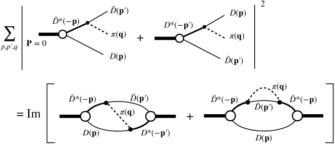
Figure 6: The optical theorem for a $D\bar{D}^{*}$ bound state decaying into $D\bar{D}\pi$.

The three-body decay is computed by the diagrams in the first (upper) line of figure 6, which are for the decay of the quasi-bound state at rest ($\bi P=0$) into $D(\bi p),\bar{D}(\bi p^{\prime}),\pi(\bi q)$. Note that there are two possible processes for a given set of the final state momenta $\bi p,\bi p^{\prime},\bi q$, whose amplitudes are added coherently. Denoting the interaction vertex of $\bar{D}^{*}\to\bar{D}\pi$ as $h\boldsymbol{\varepsilon}\cdot\bi q$, where $h=g_{A}/2f_{\pi}$ the amplitude is written as

$$\sqrt{2M_{B}}(\tilde{\varphi}(\bi p)+\tilde{\varphi}(\bi p^{\prime}))h\boldsymbol{\varepsilon}\cdot\bi q\ .$$ (115)

Here the factor $\sqrt{2M_{B}}$ is for the normalization of the initial state; there are $2M_{B}$ particles in a unit volume. Squaring this and multiplying the three-body phase space the decay rate is computed by

$$\Gamma = \frac{1}{2M_{B}}\int\frac{\rmd^{3}p}{2E_{D}(\bi p)(2\pi)^{3}}\frac{\rmd^{3}p^{\prime}}{2E_{D}(\bi p^{\prime})(2\pi)^{3}}\frac{\rmd^{3}q}{2E_{\pi}(\bi q)(2\pi)^{3}}(2\pi)^{4}\delta^{4}(p+p^{\prime}+q-P)$$ (116)

$$\times 2M_{B}h^{2}(\varphi^{*}(\bi p)+\varphi^{*}(\bi p^{\prime}))\boldsymbol{\varepsilon}^{*}\cdot\bi q\boldsymbol{\varepsilon}\cdot\bi q(\varphi(\bi p)+\varphi(\bi p^{\prime}))\ .$$

Now let us consider the diagrams of the second line of figure 6. The left diagram is computed by

$$A(M_{B}) = \int\frac{\rmd^{3}p}{2E_{D}(\bi p)(2\pi)^{3}}\frac{\rmd^{3}p^{\prime}}{2E_{D}(\bi p^{\prime})(2\pi)^{3}}\frac{\rmd^{3}q}{2E_{\pi}(\bi q)(2\pi)^{3}}(2\pi)^{3}\delta^{3}(\bi p+\bi p^{\prime}+\bi q)$$ (117)

$$\times \sqrt{2M_{B}}\tilde{\varphi}^{*}(\bi p){h\boldsymbol{\varepsilon}\cdot\bi q}\frac{1}{M_{B}-E_{D}(\bi p)-E_{D}(\bi p^{\prime})-E_{\pi}(\bi q)+i\epsilon}{h\boldsymbol{\varepsilon}\cdot\bi q}\sqrt{2M_{B}}\tilde{\varphi}(\bi p^{\prime})$$

$$= 2M_{B}h^{2}\int\frac{\rmd^{3}p}{2E_{D}(\bi p)(2\pi)^{3}}\frac{\rmd^{3}p^{\prime}}{2E_{D}(\bi p^{\prime})(2\pi)^{3}}\frac{\rmd^{3}q}{2E_{\pi}(\bi q)(2\pi)^{3}}(2\pi)^{3}\delta^{3}(\bi p+\bi p^{\prime}+\bi q)$$

$$\hskip 28.45274pt\times\;\tilde{\varphi}^{*}(\bi p)\frac{\boldsymbol{\varepsilon}^{*}\cdot\bi q\boldsymbol{\varepsilon}\cdot\bi q}{M_{B}-E_{D}(\bi p)-E_{D}(\bi p^{\prime})-E_{\pi}(\bi q)+i\epsilon}\tilde{\varphi}(\bi p^{\prime})\ .$$

Here we have used the time ordered perturbation theory and taken into account only the terms that contribute to the decay. Similarly we obtain the amplitude for the right diagram by the replacement $\varphi(\bi p^{\prime})\to\varphi(\bi p)$ in the numerator. Therefore the sum of the diagrams is

$$A(M_{B}) = 2M_{B}h^{2}\int\frac{\rmd^{3}p}{2E_{D}(\bi p)(2\pi)^{3}}\frac{\rmd^{3}p^{\prime}}{2E_{D}(\bi p^{\prime})(2\pi)^{3}}\frac{\rmd^{3}q}{2E_{\pi}(\bi q)(2\pi)^{3}}(2\pi)^{3}\delta^{3}(\bi p+\bi p^{\prime}+\bi q)$$ (118)

$$\hskip 28.45274pt\times\;\frac{(\varphi^{*}(\bi p)+\varphi^{*}(\bi p^{\prime}))\boldsymbol{\varepsilon}\cdot\bi q\boldsymbol{\varepsilon}\cdot\bi q(\varphi(\bi p)+\varphi(\bi p^{\prime}))}{M_{B}-E_{D}(\bi p)-E_{D}(\bi p^{\prime})-E_{\pi}(\bi q)+i\epsilon}\frac{1}{2}\ .$$

Picking up the imaginary part, we find

$${\rm Im}\ A(M_{B}) = -\frac{M_{B}}{2}h^{2}\int\frac{\rmd^{3}p}{2E_{D}(\bi p)(2\pi)^{3}}\frac{\rmd^{3}p^{\prime}}{2E_{D}(\bi p^{\prime})(2\pi)^{3}}\frac{\rmd^{3}q}{2E_{\pi}(\bi q)(2\pi)^{3}}(2\pi)^{4}\delta^{4}(p+p^{\prime}+q-P)$$ (119)

$$\hskip 28.45274pt\times\;(\varphi^{*}(\bi p)+\varphi^{*}(\bi p^{\prime}))\boldsymbol{\varepsilon}\cdot\bi q\boldsymbol{\varepsilon}\cdot\bi q(\varphi(\bi p)+\varphi(\bi p^{\prime}))\ .$$

The optical theorem says that by writing the $S$-matrix as $S=1-iT$,

$$S^{\dagger}S=1\to 2{\rm Im}T=|T|^{2}\ .$$ (120)

Therefore, considering the normalization of this particle ($2M_{B}$ particles in a unit volume), we find that the imaginary part agrees with the decay width. This is nothing but an explicit check of the optical theorem.

We see that the off diagonal integral in (119), $\varphi^{*}(\bi p)\cdots\varphi(\bi p^{\prime}),$ agrees with the the potential matrix element (114) modulo a kinematical factor. The difference appears due to different normalization factors in the state decaying into two particles and that of bound states. The diagonal part $\varphi^{*}(\bi p)\cdots\varphi(\bi p)$ corresponds to the imaginary part of the self energy of $\bar{D}^{*}$ and is not included in the potential matrix element.

3.7 The quark model and the hadronic model

Here we define meson and exotic states using a quark model. By doing so, we can combine the quark model and the hadron model smoothly into a quark-hadron hybrid model. Such a model enables us to handle the physics of resonances, long range interactions like OPEP, and rather complicated systems, by a hadron model but with the quark degrees of freedom effectively included. Also, by constructing hadrons from the quark degrees of freedom, the charge conjugation of the hadron systems can be defined in a more consistent way as shown below.

To obtain observables from the model Lagrangian, one has to choose the initial and/or the final state. A $q_{\alpha}\bar{{q}}_{\beta}$ meson with a certain spin structure can be defined by using the fermion bilinear as [62]

$$|q_{\alpha}\bar{q}_{\beta};\tilde{n}\Gamma\rangle = \sqrt{2M\over 2m_{\alpha}2m_{\beta}}~{}\phi~{}\tilde{n}^{*}\cdot\Big{(}\bar{\psi}_{\alpha}\;\Gamma\;\psi_{\beta}\Big{)}|0\rangle~{},$$ (121)

where $\psi_{\alpha}$ is the field operator, $\Gamma$ stands for the sixteen 4$\times$4 matrices, $\tilde{n}$ stands for the spin orientation of the state, and the mark ${\tilde{n}}^{*}$ corresponds to the complex conjugate of $\tilde{n}$. For a vector meson, $\tilde{n}^{*}\cdot(\bar{\psi}\Gamma\psi)$ corresponds to ${1\over\sqrt{2}}{\bi\epsilon}^{*}_{\mu}(\bar{\psi}\gamma^{\mu}\psi)$, and for a pseudoscalar meson, it corresponds to $({-i\over\sqrt{2}})(\bar{\psi}i\gamma^{5}\psi)$. The suffix $\alpha$ or $\beta$ stands for other quantum numbers, such as color and flavor. $\phi$ is a relative motion wave function of the quark and the antiquark. $M$ is the meson mass while $m_{\alpha}$ and $m_{\beta}$ are the quark and the antiquark masses. The normalization of this state is taken as $\langle q_{\alpha^{\prime}}\bar{q}_{\beta^{\prime}}|q_{\alpha}\bar{q}_{\beta}\rangle=2M\delta_{\alpha^{\prime}\alpha}\delta_{\beta^{\prime}\beta}(2\pi)^{3}\delta^{3}({\bi K}^{\prime}-{\bi K})$, where $\bi K$ and $\bi K^{\prime}$ are the center of mass momenta of the initial and final $q\bar{q}$ mesons, which we set to be zero in the following. The above expression can be reduced to

$$|q_{\alpha}\bar{q}_{\beta};\tilde{n}\Gamma{\bi r}\rangle =\sqrt{2M\over 2m_{\alpha}2m_{\beta}} \int{{\rm d}^{3}{\bi k}\over(2\pi)^{3}}e^{-i{\bi k}{\bi r}}\phi({\bi k})$$ (122)

$$\times\tilde{n}^{*}\cdot\sum_{s,t}\Big{(}{\bar{u}}^{s}_{\alpha}(k)\Gamma v^{t}_{\beta}(-k)\Big{)}{a}^{s}_{\alpha,{\bi k}}{}^{\dagger}b^{t}_{\beta,-{\bi k}}{}^{\dagger}|0\rangle~{},$$

where ${\bi r}={\bi r}_{q}-{\bi r}_{\bar{q}}$. Note that in this definition the ${a}^{s}{}^{\dagger}$ operator stays always on the left side of the $b^{t}{}^{\dagger}$ operator, not vice versa, for the $q\bar{q}$ meson.

Charge conjugation, $C$, changes the creation operators of the quarks to those of the antiquarks:

$$C{a}^{s}_{\alpha,{\bi k}}{}^{\dagger}C={b}^{s}_{\alpha,{\bi k}}{}^{\dagger}~{},~{}~{}~{}C{b}^{s}_{\alpha,{\bi k}}{}^{\dagger}C={a}^{s}_{\alpha,{\bi k}}{}^{\dagger}~{}.$$ (123)

So, the state $|q_{\alpha}\bar{q}_{\beta};\tilde{n}\Gamma\rangle$ is transformed into

$$C|q_{\alpha}\bar{q}_{\beta};\tilde{n}\Gamma{\bi r}\rangle = \sqrt{2M\over 2m_{\alpha}2m_{\beta}}\int{{\rm d}^{3}{\bi k}\over(2\pi)^{3}}\rme^{+\rmi{\bi k}{\bi r}}\phi({\bi k})$$ (124)

$$\times\tilde{n}^{*}\cdot\sum_{s,t}\Big{(}{\bar{u}}_{\alpha}^{s}(k)\Gamma v^{t}_{\beta}(-k)\Big{)}{b}^{s}_{\alpha,{\bi k}}{}^{\dagger}a^{t}_{\beta,-{\bi k}}{}^{\dagger}|0\rangle$$

$$= \sqrt{2M\over 2m_{\alpha}2m_{\beta}}\int{{\rm d}^{3}{\bi k}\over(2\pi)^{3}}e^{-i{\bi k}{\bi r}}\phi(-{\bi k})$$

$$\times\tilde{n}^{*}\cdot\sum_{s,t}\Big{(}{\bar{u}}_{\alpha}^{s}(-k)\Gamma v^{t}_{\beta}(k)\Big{)}{b}^{s}_{\alpha,-{\bi k}}{}^{\dagger}a^{t}_{\beta,{\bi k}}{}^{\dagger}|0\rangle$$

$$= -\sqrt{2M\over 2m_{\alpha}2m_{\beta}}\int{{\rm d}^{3}{\bi k}\over(2\pi)^{3}}e^{-i{\bi k}{\bi r}}(-1)^{\ell}\phi({\bi k})$$

$$\times\tilde{n}^{*}\cdot\sum_{s,t}\Big{(}{\bar{u}}_{\beta}^{t}(k)\gamma^{0}\gamma^{2}\Gamma^{T}\gamma^{2}\gamma^{0}v^{s}_{\alpha}(-k)\Big{)}a^{t}_{\beta,{\bi k}}{}^{\dagger}{b}^{s}_{\alpha,-{\bi k}}{}^{\dagger}|0\rangle~{}.$$

Here the coordinate ${\bi r}$ is changed to $-{\bi r}$ after the charge conjugation because it is defined as ${\bi r}_{q}-{\bi r}_{\bar{q}}$. The minus sign in the last equation comes from anticommutation of the fermion operators $a^{\dagger}$ and ${b}^{\dagger}$. There we also use

$${\bar{u}}^{s}(k) = i(\gamma^{2}\gamma^{0}v^{s}(k))^{T},{\rm~{}~{}~{}and~{}~{}~{}}v^{s}(k)=-i({\bar{u}}^{s}(k)\gamma^{0}\gamma^{2})^{T}~{}.$$ (125)

For simplicity, let us omit the orbital part of the wave function, $\phi$, and assume $\ell=0$. In a nonrelativistic quark model, the higher order term of $O(p/m)$ in the spinors is usually taken care of in operators as relativistic effects. For further computations here, we follow the convention of [62]. The nonrelativistic spinors are taken as

$$u^{s}(k)=\sqrt{m}\left(\begin{array}[]{c}\xi^{s}\\ \xi^{s}\end{array}\right){\rm~{}and~{}}v^{s}(k)=\sqrt{m}\left(\begin{array}[]{c}\xi^{-s}\\ -\xi^{-s}\end{array}\right),$$ (130)

$$\xi^{-s}=-i\sigma_{y}(\xi^{s})^{*},$$ (131)

$$\xi^{1}=\left(\begin{array}[]{c}1\\ 0\end{array}\right),\xi^{2}=\left(\begin{array}[]{c}0\\ 1\end{array}\right),$$ (136)

$$\xi^{-1}=\left(\begin{array}[]{c}0\\ 1\end{array}\right){\rm~{}and~{}}\xi^{-2}=\left(\begin{array}[]{c}-1\\ 0\end{array}\right),$$ (141)

where spin up and down correspond to $s$ = 1 and 2, respectively, for both of quarks and antiquarks.

First let us consider the pseudoscalar $Q\bar{q}$ meson, $|Q\bar{q};SS_{z}\rangle=|Q\bar{q};00\rangle$, and its behavior under the charge conjugation. For a pseudoscalar meson we take $\Gamma=i\gamma^{5}$ and $\tilde{n}=i/\sqrt{2}$ in (122),

$${1\over\sqrt{2M}}|Q\bar{q};00\rangle = {-i\over\sqrt{2}}{1\over\sqrt{2m_{Q}2m_{q}}}\sum_{s,t}\Big{(}{\bar{u}}^{s}_{Q}i\gamma^{5}v^{t}_{q}\Big{)}{a}^{s}_{Q}{}^{\dagger}b^{t}_{q}{}^{\dagger}|0\rangle~{}.$$ (142)

Then we have

$${1\over\sqrt{2M}}|Q\bar{q};00\rangle = {-i\over\sqrt{2}}(-i)\sum_{s,t}\xi^{s}{}^{\dagger}\xi^{-t}{a}^{s}_{Q}{}^{\dagger}b^{t}_{q}{}^{\dagger}|0\rangle$$ (143)

$$= -{1\over\sqrt{2}}\Big{(}\xi^{1}{}^{\dagger}\xi^{-2}{a}^{1}_{Q}{}^{\dagger}b^{2}_{q}{}^{\dagger}+\xi^{2}{}^{\dagger}\xi^{-1}{a}^{2}_{Q}{}^{\dagger}b^{1}_{q}{}^{\dagger}\Big{)}|0\rangle$$

$$= -{1\over\sqrt{2}}\Big{(}-{a}^{1}_{Q}{}^{\dagger}b^{2}_{q}{}^{\dagger}+{a}^{2}_{Q}{}^{\dagger}b^{1}_{q}{}^{\dagger}\Big{)}|0\rangle$$

$$= {1\over\sqrt{2}}\Big{(}|Q^{\uparrow}\bar{q}^{\downarrow}\rangle-|Q^{\downarrow}\bar{q}^{\uparrow}\rangle\Big{)}.$$

This corresponds to the $D$ meson when $Q$ and $q$ are taken as the charm and the light quarks, respectively. In the last equation, we define $|q\rangle=a^{\dagger}|0\rangle$ so that its normalization becomes 1 instead of $2E$ as in the nonrelativistic quark model.

When charge conjugation is applied to this state, we have

$$C{1\over\sqrt{2M}}|Q\bar{q};00\rangle = -{-i\over\sqrt{2}}{1\over\sqrt{2m_{Q}2m_{q}}}\sum_{s,t}\Big{(}{\bar{u}}^{t}_{q}\gamma^{0}\gamma^{2}i(\gamma^{5})^{T}\gamma^{2}\gamma^{0}v^{s}_{Q}\Big{)}{a}^{t}_{q}{}^{\dagger}b^{s}_{Q}{}^{\dagger}|0\rangle$$ (144)

$$= {-i\over\sqrt{2}}{1\over\sqrt{2m_{Q}2m_{q}}}\Big{(}{\bar{u}}^{t}_{q}i\gamma^{5}v^{s}_{Q}\Big{)}{a}^{t}_{q}{}^{\dagger}b^{s}_{Q}{}^{\dagger}|0\rangle$$

$$= {1\over\sqrt{2}}\Big{(}|q^{\uparrow}\bar{Q}^{\downarrow}\rangle-|q^{\downarrow}\bar{Q}^{\uparrow}\rangle\Big{)}$$

$$= +{1\over\sqrt{2M}}|q\bar{Q};00\rangle~{}.$$

This state can be regarded as the $\bar{D}$ meson, meaning that the charge conjugate of the $D$ meson is ($+1$) times the $\bar{D}$ meson. Or, when both of the $Q$ and $q$ quarks are taken to be the charm quarks, this state corresponds to the $\eta_{c}$ meson, whose $C$-parity is ($+1$).

Next we consider the vector meson, $|Q\bar{q};SS_{z}\rangle=|Q\bar{q};11\rangle$, and its behavior under charge conjugation. Now we take $\tilde{n}$ to be ${{\bi\epsilon}^{+}/\sqrt{2}}={1\over 2}(0,1,-i,0)^{\mu}$ and $\Gamma=\gamma^{\mu}$.

$${1\over\sqrt{2M}}|Q\bar{q};11\rangle = {1\over 2}(0,1,i,0)_{\mu}{1\over\sqrt{2m_{Q}2m_{q}}}\sum_{s,t}\Big{(}{\bar{u}}^{s}_{Q}\gamma^{\mu}v^{t}_{q}\Big{)}{a}^{s}_{Q}{}^{\dagger}b^{t}_{q}{}^{\dagger}|0\rangle~{}.$$ (145)

Then we have

$${1\over\sqrt{2M}}|Q\bar{q};11\rangle = \sum_{s,t}\xi^{s}{}^{\dagger}{1\over 2}(\sigma_{x}+i\sigma_{y})\xi^{-t}{a}^{s}_{Q}{}^{\dagger}b^{t}_{q}{}^{\dagger}|0\rangle$$ (146)

$$= \xi^{1}{}^{\dagger}\xi^{-1}{a}^{1}_{Q}{}^{\dagger}b^{1}_{q}{}^{\dagger}|0\rangle={a}^{1}_{Q}{}^{\dagger}b^{1}_{q}{}^{\dagger}|0\rangle,$$

$$= |Q^{\uparrow}\bar{q}^{\uparrow}\rangle~{},$$

which corresponds to the $D^{*}$ meson, when $Q$ and $q$ are the charm and nonflavor quarks, respectively. Under the charge conjugation, it becomes

$$C{1\over\sqrt{2M}}|Q\bar{q};11\rangle = -{1\over 2}(0,1,i,0)_{\mu}$$ (147)

$$\times{1\over\sqrt{2m_{Q}2m_{q}}}\sum_{s,t}\Big{(}{\bar{u}}^{t}_{q}\gamma^{0}\gamma^{2}(\gamma^{\mu})^{T}\gamma^{2}\gamma^{0}v^{s}_{Q}\Big{)}{a}^{t}_{q}{}^{\dagger}b^{s}_{Q}{}^{\dagger}|0\rangle$$

$$= -{1\over 2}(0,1,i,0)_{\mu}{1\over\sqrt{2m_{Q}2m_{q}}}\sum_{s,t}\Big{(}{\bar{u}}^{t}_{q}\gamma^{\mu}v^{s}_{Q}\Big{)}{a}^{t}_{q}{}^{\dagger}b^{s}_{Q}{}^{\dagger}|0\rangle$$

$$= -{a}^{1}_{q}{}^{\dagger}b^{1}_{Q}{}^{\dagger}|0\rangle$$

$$= -|q^{\uparrow}\bar{Q}^{\uparrow}\rangle~{}.$$

This corresponds to ($-1$) times the ${\bar{D}}{}^{*}$ meson. Or, when both of the $Q$ and $q$ quarks are taken to be the charm quarks, this state corresponds to the $J/\psi$ meson, whose $C$-parity is ($-1$). This result and (144) are in accordance with what has been anticipated in (24).

Finally, we consider a four-quark system such as $D^{(*)}\bar{D}{}^{(*)}$ and its charge conjugation. The $C$-parity can be defined for the neutral systems. The charge conjugation changes $D$ to $\bar{D}$, and $D^{*}$ to $-{\bar{D}}{}^{*}$. Thus the $C$-parity changes $D^{(*)}\bar{D}{}^{(*)}$ associated with the orbital relative wave function, $\psi_{L}({\bi r})$, with ${\bi r}={\bi r}_{D}-{\bi r}_{\bar{D}}$, as

$$C:~{}D{\bar{D}}\psi_{L}({\bi r}) \to {\bar{D}}D\psi_{L}(-{\bi r})=(-1)^{L}D{\bar{D}}\psi_{L}({\bi r}),$$ (148)

$$C:~{}D{\bar{D}}{}^{*}\psi_{L}({\bi r}) \to {-{\bar{D}}}D^{*}\psi_{L}(-{\bi r})=-(-1)^{L}D^{*}{\bar{D}}\psi_{L}({\bi r}),$$ (149)

$$C:~{}D{}^{*}{\bar{D}}\psi_{L}({\bi r}) \to {-{\bar{D}}{}^{*}}D\psi_{L}(-{\bi r})=-(-1)^{L}D{\bar{D}}{}^{*}\psi_{L}({\bi r}),$$ (150)

$$C:~{}D^{*}{\bar{D}}{}^{*}\psi_{L}({\bi r}) \to {\bar{D}}{}^{*}D^{*}\psi_{L}(-{\bi r})=(-1)^{L+S}D^{*}{\bar{D}}{}^{*}\psi_{L}({\bi r}),$$ (151)

where $L$ is the orbital angular momentum of the $D^{(*)}$ and $\bar{{D}}^{(*)}$ relative motion, and $S$ is the total spin $(=0,1,2)$. Thus, the $C$-parity eigenstates of the $D{\bar{D}}$ systems are also eigenstates of the parity,

$$J^{PC} = L^{++}:[D\bar{D}]_{+}\psi_{L=even}$$ (153)

$$L^{--}:[D\bar{D}]_{-}\psi_{L=odd}$$

with

$${}[D\bar{D}]_{\pm} = {1\over\sqrt{2}}\Big{(}D{\bar{D}}\pm{\bar{D}}D\Big{)}~{}.$$ (154)

Similarly, those with $D{\bar{D}}{}^{*}$ or $D^{*}{\bar{D}}$ are

$$J^{PC} = J^{++}:{1\over\sqrt{2}}\Big{(}[D{\bar{D}}{}^{*}]_{-}-[D{}^{*}{\bar{D}}]_{-}\Big{)}\psi_{L=even},$$ (158)

$$J^{+-}:{1\over\sqrt{2}}\Big{(}[D{\bar{D}}{}^{*}]_{+}+[D{}^{*}{\bar{D}}]_{+}\Big{)}\psi_{L=even},$$

$$J^{-+}:{1\over\sqrt{2}}\Big{(}[D{\bar{D}}{}^{*}]_{-}+[D{}^{*}{\bar{D}}]_{-}\Big{)}\psi_{L=odd},$$

$$J^{--}:{1\over\sqrt{2}}\Big{(}[D{\bar{D}}{}^{*}]_{+}-[D{}^{*}{\bar{D}}]_{+}\Big{)}\psi_{L=odd}$$

with

$${}[D{\bar{D}}{}^{*}]_{\pm} = {1\over\sqrt{2}}(D{\bar{D}}{}^{*}\pm{\bar{D}}D^{*}),~{}~{}~{}{}[D{}^{*}{\bar{D}}]_{\pm}={1\over\sqrt{2}}(D^{*}{\bar{D}}\pm{\bar{D}}{}^{*}D)~{}.$$ (159)

For $D^{*}{\bar{D}}{}^{*}$, the simultaneous eigenstates of the parity and the $C$-parity relate to the angular momentum $L$ and the total spin $S$ as

$$J^{PC} = J^{++}:[D^{*}{\bar{D}}{}^{*}]_{S=even,+}\psi_{L=even},$$ (163)

$$J^{+-}:[D^{*}{\bar{D}}{}^{*}]_{S=odd,-}\psi_{L=even},$$

$$J^{-+}:[D^{*}{\bar{D}}{}^{*}]_{S=odd,+}\psi_{L=odd},$$

$$J^{--}:[D^{*}{\bar{D}}{}^{*}]_{S=even,-}\psi_{L=odd}$$

with

$${}[D{}^{*}\bar{D}{}^{*}]_{S,\pm} = {1\over\sqrt{2}}\Big{(}D{}^{*}{\bar{D}}{}^{*}\pm{\bar{D}}{}^{*}D{}^{*}\Big{)}\Big{|}_{S}~{}.$$ (164)

In the quark model, the relations concerning the rearrangement between $c\bar{c}$-$q\bar{q}$ and $c\bar{q}$-$q\bar{c}$ are derived in a systematic manner. For this, first we note that there are two color configurations for the $q\bar{{q}}c\bar{{c}}$ systems: the one where the quark-antiquark pairs $q\bar{{q}}$ and $c\bar{{c}}$ are color singlet and the other where the pairs $q\bar{{c}}$ and $c\bar{{q}}$ are color singlet. These two configurations are related to hidden charm, $\omega J\!/\!\psi$ etc., and open charm $D^{(*)}\bar{{D}}{}^{(*)}$ configurations, respectively. They are two independent bases although they are not orthogonal to each other from the quark model point of view. In fact, they are related by rearrangement factors. The color rearrangement factor is 1/3. In the following we demonstrate the rearrangement for the spin and isospin parts and omit the color factor for simplicity.

The spin rearrangement factor of the $q\bar{{q}}c\bar{{c}}$ $S$-wave system can be obtained as

$$|(s_{12}s_{34})SM\rangle = \sum_{s_{14},s_{32}}(-1)^{-s_{12}-s_{32}}\sqrt{(2s_{12}+1)(2s_{34}+1)(2s_{14}+1)(2s_{32}+1)}$$ (168)

$$\times\left\{\begin{array}[]{ccc}{1\over 2}&{1\over 2}&s_{12}\\ {1\over 2}&{1\over 2}&s_{34}\\ s_{32}&s_{14}&S\\ \end{array}\right\}|(s_{32}s_{14})SM\rangle,$$

where $s_{ij}=s_{i}+s_{j}$ with the spin of $i$th quark $s_{i}$, the total spin $S$ corresponds to $S=\sum_{i}s_{i}=s_{12}+s_{34}=s_{14}+s_{32}$, and the array with the braces is the 9-$J$ symbol. The factor $(-1)^{-s_{12}-s_{32}}$ appears because we define the mesons by the $q\bar{{q}}$ (not $\bar{{q}}q$) states. The numerical factors are listed in table 5 together with the two meson states for the isospin 0 systems. The table shows, for example, that the rearrangement of $\eta\eta_{c}$ ($J^{PC}=0^{++}$) consists of $[D\bar{{D}}]_{+}$ and the total spin-0 $[D^{*}\bar{{D}}{}^{*}]_{0,+}$ states in the spin space as

$$\eta\eta_{c}(0^{++})={1\over 2}[D\bar{{D}}]_{+}-{\sqrt{3}\over 2}[D^{*}\bar{{D}}{}^{*}]_{0,+}.$$ (169)

One can see in table 5 that the above relation between $J^{PC}$ and the phase in (153)–(164) appears for each $C$-parity.

Table 5: Rearrangement of the $q\bar{{q}}$-$c\bar{{c}}$-type mesons and $D\bar{{D}}$ mesons. The definition of $[D{}^{(*)}\bar{{D}}{}^{(*)}]$ are shown in (154), (159) and (164). $[D\bar{{D}}{}^{*}]_{\pm}$ means $[D\bar{{D}}{}^{*}]_{+}$ for $J^{PC}=1^{+-}$, and $[D\bar{{D}}{}^{*}]_{-}$ for $1^{++}$. The quark configuration of the $\eta$ meson is assumed to be $(u\bar{{u}}+d\bar{{d}})/\sqrt{2}$.

$J^{PC}$		$[D\bar{{D}}]_{+}$	$[D^{*}\bar{{D}}{}^{*}]_{S=0,+}$	$[D\bar{{D}}{}^{*}]_{\pm}$	$[D^{*}\bar{{D}}]_{\pm}$	$[D^{*}\bar{{D}}{}^{*}]_{S=1,-}$	$[D^{*}\bar{{D}}{}^{*}]_{S=2,+}$
$0^{++}$	$\eta\eta_{c}$	${1\over 2}$	$-{\sqrt{3}\over 2}$
$0^{++}$	$\omega J\!/\!\psi$	$-{\sqrt{3}\over 2}$	$-{1\over 2}$
$1^{+-}$	$\eta J\!/\!\psi$			${1\over 2}$	${1\over 2}$	$-\sqrt{1\over 2}$
$1^{+-}$	$\omega\eta_{c}$			${1\over 2}$	${1\over 2}$	$\sqrt{1\over 2}$
$1^{++}$	$\omega J\!/\!\psi$			$-\sqrt{1\over 2}$	$\sqrt{1\over 2}$	$0$
$2^{++}$	$\omega J\!/\!\psi$						1

Up to now, the $D$ meson corresponds to $c\bar{{q}}$ and the $\bar{{D}}$ meson to $q\bar{{c}}$. The neutral $D\bar{{D}}$ states consist of the isospin 0 and 1 states, $((c\bar{{u}}u\bar{{c}})+(c\bar{{d}}d\bar{{c}}))/\sqrt{2}$ and $((c\bar{{u}}u\bar{{c}})-(c\bar{{d}}d\bar{{c}}))/\sqrt{2}$, respectively. Using relation (100), we replace the $c\bar{{q}}$-$q\bar{{c}}$ expression, $[D^{(*)}\bar{{D}}{}^{(*)}]_{\pm}$, by

$$-\sqrt{1\over 2}\Big{(}[D^{(*)+}D{}^{(*)-}]_{\pm}-[D^{(*)0}\bar{{D}}{}^{(*)0}]_{\pm}\Big{)}~{}~{}~{}(I=0)$$ (170)

$$+\sqrt{1\over 2}\Big{(}[D^{(*)+}D{}^{(*)-}]_{\pm}+[D^{(*)0}\bar{{D}}{}^{(*)0}]_{\pm}\Big{)}~{}~{}~{}(I=1).$$ (171)

In the next section we discuss the $X$(3872), whose $J^{PC}=1^{++}$. The rearrangement becomes

$$\omega J\!/\!\psi(1^{++}) = -\sqrt{1\over 2}[D\bar{{D}}{}^{*}]_{-}+\sqrt{1\over 2}[D^{*}\bar{{D}}]_{-},$$ (172)

which, if the state has isospin 0, becomes

$${1\over 2}\Big{(}([D^{+}D{}^{*-}]_{-}-[D^{0}\bar{{D}}{}^{*0}]_{-})-([D^{*+}D{}^{-}]_{-}-[D^{*0}\bar{{D}}{}^{0}]_{-})\Big{)}.$$ (173)

We will denote above state simply by $(D\bar{D}{}^{*}-D^{*}{\bar{{D}}})/\sqrt{2}$, or just by $D\bar{D}{}^{*}$ in the isospin basis if there is no room for confusion. Or, in the following section on $X(3872)$, when we write $D^{+}D{}^{*-}$ and $D^{0}\bar{{D}}{}^{*0}$ in the particle basis, they mean

$${1\over\sqrt{2}}([D^{+}D{}^{*-}]_{-}-[D^{*+}D{}^{-}]_{-})~{}~{}{\rm and}~{}~{}{1\over\sqrt{2}}([D^{0}\bar{{D}}{}^{*0}]_{-}-[D^{*0}\bar{{D}}{}^{0}]_{-}),$$ (174)

respectively. So, by this notation, the isospin eigenstates of $I(J^{PC})=0(1^{++})$ are

$$\sqrt{1\over 2}\Big{(}D^{+}D{}^{*-}-D^{0}\bar{{D}}{}^{*0}\Big{)}$$ (175)

as usual.

In much of the literature on hadron models, such as [63, 64], the charge conjugate of $D^{*}$ is defined as ${\bar{D}}{}^{*}$, not $-{\bar{D}}{}^{*}$. This can be realized when the $\bar{{D}}{}^{(*)}$ meson is taken to be ${\bar{c}}q$, not $q\bar{c}$. In such a hadron model, the $C$-parity $\pm 1$ eigenstates are given by $(D{\bar{D}}{}^{*}\pm D^{*}{\bar{D}})/\sqrt{2}$, respectively. This difference in the phase is due only to the definition. An extra factor appears when the observables are calculated, which compensates for the above difference.

4 $X$(3872)

4.1 The observed features of $X$(3872)

The $X$(3872) state (also $\chi_{c1}(3872)$) was first observed in 2003 by Belle in the weak decay of the $B$ meson, $B^{\pm}\to J/\psi\,\pi^{+}\,\pi^{-}\,K^{\pm}$ [1] and was confirmed by CDF [65], D0 [66], $BABAR$ [67], LHCb [68], CMS [69] ATLAS [70] and BESIII [71] collaborations. Since then a considerable amount of $X$(3872)-related data has been accumulated. We summarize major experimental data samples in Table 6.

The observed mass of $X$(3872) extracted from the $B\to J/\psi\,\pi^{+}\pi^{-}K$ mode in the recent measurement is $3871.85\pm 0.27\pm 0.19$ MeV [72]. Those from the $p\bar{p}$ and the $pp$ collisions in the final state $J/\psi\pi^{+}\pi^{-}+$ anything are $3871.61\pm 0.16\pm 0.19$ MeV [73] and $3871.95\pm 0.48\pm 0.12$ MeV [68], respectively. The average mass given by the particle data group in 2018 [5] in the $J/\psi X$ modes is $3871.69\pm 0.17$ MeV, which is $0.01\pm 0.19$ MeV above the $D^{0}\mbox{$\bar{D}^{\ast 0}$}$ threshold 3871.68 MeV.

The observed masses of the $X$(3872) in the $B\to\mbox{$\bar{D}^{\ast 0}$}D^{0}K$ decay mode are $3872.9^{+0.6}_{-0.4}{}^{+0.4}_{-0.5}$ MeV by Belle [74] and $3875.1^{+0.7}_{-0.5}\pm 0.5$ MeV by $BABAR$ [75]. The observed mass of the $X$(3872) in the $B\to D^{0}\bar{D}^{0}\pi^{0}K$ decay mode is $3875.2\pm 0.7^{+0.9}_{-1.8}$ MeV [76]. The masses observed in the $B\to\mbox{$\bar{D}^{\ast 0}$}D^{0}K$ and $B\to D^{0}\bar{D}^{0}\pi^{0}K$ decay mode are heavier than those in the $J/\psi X$ modes.

The full width is less than 1.2 MeV [72]. The observed full widths of the charmonia in the same energy region as the $X(3872)$ are $27.2\pm 1.0$ MeV for $\psi(3770)$, $11.3^{+3.2}_{-2.9}$ MeV for $\eta_{c}(2S)$, $201^{+154}_{-67}{}^{+88}_{-82}$ MeV for $\chi_{c0}(3860)$ and $24\pm 6$ MeV for $\chi_{c2}(3930)$ [5]. Therefore the width of $X(3872)$ is unusually small as compared with the other charmonia, which is one of the striking features of the $X(3872)$.

As for the spin-parity quantum numbers of the $X$(3872), the angular distributions and correlations of the $\pi^{+}\pi^{-}J/\psi$ final state have been studied by CDF [77]. They concluded that the pion pairs originate from $\rho^{0}$ mesons and that the favored quantum numbers of the $X$(3872) are $J^{PC}=1^{++}$ and $2^{-+}$. The radiative decays of $X(3872)\to\gamma J/\psi$ have been observed [78, 79, 80, 81], which implies that the $C$-parity of $X$(3872) is positive. Finally, LHCb performed an analysis of the angular correlations in $B^{+}\to X(3872)K^{+}$, $X(3872)\to\pi^{+}\pi^{-}J/\psi$, $J/\psi\to\mu^{+}\mu^{-}$ decays and confirmed the eigenvalues of total spin angular momentum, parity and charge conjugation of the $X(3872)$ state to be $1^{++}$ [4, 82].

Table 6: Experimental status of $X(3872)$. In the fourth and fifth columns, short notations are employed. S($\sigma$) means the significance in unit of $\sigma$ and OQ means Observed quantities. M, W, BF and CS mean Mass, Width, Branching Fraction and Cross Section, respectively.

Exp.	Mode	Yield	S($\sigma$)	OQ	Ref.
Belle	$B^{\pm}\to X(3872)(\to J/\psi\pi^{+}\pi^{-})K^{\pm}$	$35.7\pm 6.8$	10.3	M, W	[1]
	$B\to X(3872)(\to D^{\ast 0}\bar{D}^{0})K$	$50.1^{+14.8}_{-11.1}$	6.4	M, W, BF	[74]
	$B^{+}\to X(3872)(\to J/\psi\gamma)K^{+}$	$30.0^{+8.2}_{-7.4}$	4.9	BF	[80]
	$B^{0}\to X(3872)(\to J/\psi\gamma)K^{0}_{S}$	$5.7^{+3.5}_{-2.8}$	2.4	BF	[80]
	$B^{+}\to X(3872)(\to J/\psi\pi^{+}\pi^{-})K^{+}$	$152\pm 15$		M, W, BF	[72]
	$B^{0}\to X(3872)(\to J/\psi\pi^{+}\pi^{-})K^{0}_{S}$	$21.0\pm 5.7$	6.1	M, W, BF	[72]
CDF II	$J/\psi\pi^{+}\pi^{-}$ in $p\bar{p}$ at $\sqrt{S}=1.96$ TeV	$730\pm 90$	11.6	M, W	[65]
CDF	$J/\psi\pi^{+}\pi^{-}$ in $p\bar{p}$ at $\sqrt{S}=1.96$ TeV			$J^{PC}$	[77]
D0	$J/\psi\pi^{+}\pi^{-}$ in $p\bar{p}$ at $\sqrt{S}=1.96$ TeV	$522\pm 100$	5.2	M	[66]
BABAR	$B^{-}\to X(3872)(\to J/\psi\pi^{+}\pi^{-})K^{-}$	$25.4\pm 8.7$		M, BF	[67]
	$B^{+}\to X(3872)(\to J/\psi\gamma)K^{+}$	$19.2\pm 5.7$	3.4	BF	[78]
	$B^{+}\to X(3872)(\to D^{\ast 0}\bar{D}^{0})K^{+}$	$27.4\pm 5.9$	4.6	BF	[75]
	$B^{0}\to X(3872)(\to D^{\ast 0}\bar{D}^{0})K^{0}_{S}$	$5.8\pm 2.7$	1.3	BF	[75]
	$B^{+}\to X(3872)(\to J/\psi\pi^{+}\pi^{-})K^{+}$	$93.4\pm 17.2$	8.6	M, W, BF	[83]
	$B^{0}\to X(3872)(\to J/\psi\pi^{+}\pi^{-})K^{0}_{S}$	$9.4\pm 5.2$	2.3	M, W, BF	[83]
	$B^{+}\to X(3872)(\to J/\psi\gamma)K^{+}$	$23.0\pm 6.4\pm 0.6$	3.6	BF	[79]
	$B^{+}\to X(3872)(\to\psi(2S)\gamma)K^{+}$	$25.4\pm 7.3\pm 0.7$	3.5	BF	[79]
LHCb	$J/\psi\pi^{+}\pi^{-}$ in $pp$ at $\sqrt{S}=7$ TeV	$565\pm 62$		M, W, CS	[68]
	$B^{+}\to X(3872)(\to J/\psi\gamma)K^{+}$	$591\pm 48$		BF	[81]
	$B^{+}\to X(3872)(\to\psi(2S)\gamma)K^{+}$	$36.4\pm 9.0$	4.4	BF	[81]
	$B^{+}\to X(3872)(\to J/\psi\rho^{0})K^{+}$	$1011\pm 38$	16	$J^{PC}$	[4, 82]
CMS	$J/\psi\pi^{+}\pi^{-}$ in $pp$ at $\sqrt{S}=7$ TeV	$11910\pm 490$		CS	[69]
ATLAS	$J/\psi\pi^{+}\pi^{-}$ in $pp$ at $\sqrt{S}=8$ TeV			CS	[70]
BESIII	$e^{+}e^{-}\to\gamma X(3872)(\to J/\psi\pi^{+}\pi^{-})$	$20.0\pm 4.6$	6.3	M, CS, BF	[71]
	$e^{+}e^{-}\to\gamma X(3872)(\to J/\psi\pi^{+}\pi^{-}\pi^{0})$	$45\pm 9\pm 3$	5.7	M, W, BF	[84]

Since the first observation of the $X$(3872), it has received much attention because its features are difficult to explain if a simple $c\bar{c}$ bound state of the quark potential model is assumed [85]. The interaction between heavy quark and heavy antiquark is well understood and known that it can be approximately expressed by a Coulomb-plus-linear potential, a feature that is confirmed by lattice QCD studies [86, 87]. The charmonium states with $J^{PC}=1^{++}$ are the $\chi_{c1}$ states. The observed mass of the ground state of the $\chi_{c1}(1P)$ is ($3510.67\pm 0.05$) MeV and the quark potential model gives similar mass [88]. The first excited state of the $\chi_{c1}$ is the $\chi_{c1}(2P)$ and that state has, so far, not been observed. The predicted mass of the $\chi_{c1}(2P)$ in quark potential models is in between $3925$ MeV and $3953$ MeV [88]. The observed mass of $X(3872)$ is 53-81 MeV smaller than these predictions. This is one of the strong grounds for the identification of the $X$(3872) as a non-ccbar structure. A variety of structures have been suggested for the $X$(3872) from the theoretical side, such as a tetraquark structure [9, 89, 10, 90, 91], $D^{0}\mbox{$\bar{D}^{\ast 0}$}$ molecule [92, 93, 63, 94, 95, 96, 97, 98, 99, 100, 101, 102, 103, 104, 105, 106, 107, 108, 109, 110] and a charmonium-molecule hybrid [111, 112, 113, 114, 115, 116, 117, 38, 118, 119]. The structure of the $X(3872)$ has also been studied with the lattice QCD approach [120, 121, 122, 123].

One of the important properties of the $X$(3872) is its isospin structure. The branching fractions measured by Belle [124] is

$$\frac{Br(X\rightarrow\pi^{+}\pi^{-}\pi^{0}J/\psi)}{Br(X\rightarrow\pi^{+}\pi^{-}J/\psi)}=1.0\pm 0.4\pm 0.3\,,$$ (176)

and $0.8\pm 0.3$ by $BABAR$ [125]. Here the two-pion mode originates from the isovector $\rho$ meson while the three-pion mode comes from the isoscalar $\omega$ meson. So, the equation (176) indicates strong isospin violation. Recently, BESIII observed $X(3872)\to\omega J/\psi$ decay with a significance of more than 5$\sigma$ and the relative decay ratio of $X(3872)\to\omega J/\psi$ and $\pi^{+}\pi^{-}J/\psi$ was measured to be ${\cal R}=1.6^{+0.4}_{-0.3}\pm 0.2$ [84]. The kinematical suppression factor including the difference of the vector meson decay width were studied [126, 127], and the production amplitude ratio [127] was obtained by using Belle’s value [124]

$$\left|\frac{A(\rho J/\psi)}{A(\omega J/\psi)}\right|=0.27\pm 0.02\,.$$ (177)

Typical size of the isospin symmetry breaking ratios is at most a few %. It is interesting to know what the origin of this strong isospin symmetry breaking is. In [98], this problem was studied using the chiral unitary model, and the effect of the $\rho$-$\omega$ mixing has been discussed in [128]. It was reported that both of these approaches can explain the observed ratio given in (176). In the charmonium-molecule hybrid approach, the difference of the $D^{0}\mbox{$\bar{D}^{\ast 0}$}$ and the $D^{+}D^{*-}$ thresholds produces sufficient isospin violation to naturally explain the experimental results [115, 38]. The Friedrichs-model-like scheme can also explain the isospin symmetry breaking [129]. Recently, a new Isospin=1 decay channel, $X(3872)\to\pi^{0}\chi_{c1}$ has been observed [130].

$X$(3872) production at high energy hadron colliders has been studied in [131, 132, 133, 134, 69, 135, 136, 137, 138, 139, 140, 141, 142, 143], where unexpectedly large production rates have been observed at large transverse momentum transfers $p_{\perp}>10$ GeV [144]. These rates are much larger than those for production of light nuclei such as the deuteron and ³He, and are about 5 % of that for the $\psi(2S)$. This property is naively explained if $X(3872)$ has a small “core” component that is a compact structure such as the $\chi_{c1}(2P)$. In a later subsection we will see that this will be realized in a model of $D\bar{D}^{*}$ molecular coupled with a $c\bar{c}$ core.

The hadronic decays of the $X$(3872) are investigated in [145, 126, 146, 147, 148, 149, 150, 151, 152, 153, 135, 154, 155, 156, 157, 158]. As for radiative decays, as seen in [159, 160, 161, 162, 163, 164, 165, 166, 167, 168, 169, 170, 171, 172, 173], the existence of a core seems to be required, but the results depend on details of the wave function.

Another important issue is whether the charged partner of $X(3872)$ exists as a measurable peak or not. $BABAR$ has searched such a state in the $X(3872)\to\pi^{-}\pi^{0}J/\psi$ channel and found no signal [2]. Belle has also studied such a state using much accumulated data but found no signal [72]. The hybrid picture, where the coupling to the $c\bar{{c}}$ core is essential to bind the neutral $X(3872)$, is consistent with the absence of a charged $X(3872)$.

Since the $X(3872)$ has many interesting properties, and many studies of it have been done, several review papers have been written from various viewpoints [174, 175, 6, 176, 177, 178, 144, 179, 180, 24].

4.2 $D^{(\ast)}\bar{D}^{(\ast)}$ molecule with OPEP

In this subsection, we demonstrate the analysis of the $X(3872)$ as a $D^{(\ast)}\bar{D}^{(\ast)}$ molecule with $I^{G}(J^{PC})=0^{+}(1^{++})$. As for the interaction between $D^{(\ast)}$ and $\bar{D}^{(\ast)}$ mesons, we employ only the OPEP in (92)-(95). In the $D^{(\ast)}\bar{D}^{(\ast)}$ coupled channel system, the possible $D^{(\ast)}\bar{D}^{(\ast)}$ components with positive charge conjugation are

$$\frac{1}{\sqrt{2}}(D\bar{D}^{\ast}-D^{\ast}\bar{D})(^{3}S_{1},{{}^{3}D_{1}}),\quad D^{\ast}\bar{D}^{\ast}(^{5}D_{1}),$$ (178)

where $(^{2S+1}L_{J})$ denotes the total spin $S$, the orbital angular momentum $L$ and the total angular momentum $J$ [12, 57]. We note that the phase convention in (178) is different from the one in the literature [12, 57] as discussed in section 3.7. In this basis, the matrix elements of the OPEP are given by [12, 57]

$$V_{\pi}(r) = \left(\frac{g_{A}}{2f_{\pi}}\right)^{2}\left(\begin{array}[]{ccc}{\cal C}_{\pi}&-\sqrt{2}{\cal T}_{\pi}&-\sqrt{6}T_{\pi}\\ -\sqrt{2}{\cal T}_{\pi}&{\cal C}_{\pi}+{\cal T}_{\pi}&-\sqrt{3}T_{\pi}\\ -\sqrt{6}T_{\pi}&-\sqrt{3}T_{\pi}&C_{\pi}-T_{\pi}\\ \end{array}\right),$$ (182)

where ${\cal C}_{\pi}=C(r;\mu,\Lambda)$, ${\cal T}_{\pi}=T(r;\mu,\Lambda)$, $C_{\pi}=C(r;m_{\pi},\Lambda)$, and $T_{\pi}=T(r;m_{\pi},\Lambda)$, respectively. The functions $C(r;m,\Lambda)$ and $T(r;m,\Lambda)$ are defined in (87) and (88). The functions ${\cal C}_{\pi}$ and ${\cal T}_{\pi}$ with $\mu$ emerge because the nonzero energy transfer in the $D$-$D^{\ast}$ transition is taken into account in the potential $V^{\pi}_{P\bar{P}^{\ast}{\mathchar 45\relax}P^{\ast}\bar{P}}(r)$ as explained in section 3.4. In the charm sector, the mass $\mu$ becomes imaginary, i.e. $\mu^{2}=m^{2}_{\pi}-(m_{D^{\ast}}-m_{D})^{2}<0$. In this subsection, the hadron masses summarized in table 7 are used, which are the isospin averaged masses. Then, $\mu^{2}=(37.3i)^{2}$ [MeV²] is obtained, and the $\cal{C}_{\pi}$ and $\cal{T}_{\pi}$ become complex as seen in (107). The explicit expression of the imaginary central and tensor potentials is given in [127]. In this analysis, we consider only the real part of the potential, because the imaginary part is small for small $\mu$.

Table 7: Hadron masses used in the numerical calculation. The masses of the pion, pseudoscalar meson $P=D,B$ and vector $P^{\ast}=D^{\ast},B^{\ast}$ meson are shown in the $ud$, charm and bottom sectors. The pion mass is given as the averaged mass of $\pi^{+}$, $\pi^{0}$ and $\pi^{-}$ [5]. The $P^{(\ast)}$ mass is the averaged mass of $P^{(\ast)0}$ and $P^{(\ast)\pm}$ [5]. The mass difference $\Delta M_{PP^{\ast}}$ between the masses of $P$ and $P^{\ast}$ is also shown. The values are in units of MeV.

	$\pi$ [MeV]
$ud$	137
	$P$ [MeV]	$P^{\ast}$ [MeV]	$\Delta M_{PP^{\ast}}$ [MeV]
charm	1867	2009	145
bottom	5279	5325	46

The Hamiltonian of the $D^{(\ast)}\bar{D}^{(\ast)}$ coupled channel system is

$$H=K+V_{\pi},$$ (183)

where the kinetic term $K$ is given by

$$K={\rm diag}\left(-\frac{1}{2\mu_{D\bar{D}^{\ast}}}\Delta_{0},-\frac{1}{2\mu_{D\bar{D}^{\ast}}}\Delta_{2},-\frac{1}{2\mu_{D^{\ast}\bar{D}^{\ast}}}\Delta_{2}+\Delta m_{DD^{\ast}}\right).$$ (184)

Here we define

$$\Delta_{\ell}=\frac{\partial^{2}}{\partial r^{2}}+\frac{2}{r}\frac{\partial}{\partial r}+\frac{\ell(\ell+1)}{r^{2}},$$ (185)

for the state of orbital angular momentum $\ell$, the reduced mass

$$\mu_{D^{(\ast)}\bar{D}^{(\ast)}}=\frac{m_{D^{(\ast)}}m_{\bar{D}^{(\ast)}}}{m_{D^{(\ast)}}+m_{\bar{D}^{(\ast)}}},$$ (186)

and

$$\Delta m_{DD^{\ast}}=m_{D^{\ast}}-m_{D}.$$ (187)

The $D^{(\ast)}\bar{D}^{(\ast)}$ systems are studied by solving the Schrödinger equation with the Hamiltonian $H$ (183). In the potential $V_{\pi}$, there are two parameters, the coupling constant $g_{A}$ and the cutoff parameter $\Lambda$. The coupling $g_{A}$ is determined by the $D^{\ast}\rightarrow D\pi$ decay as shown in section 2.3. The cutoff $\Lambda$ is a free parameter, while it can be evaluated by the ratio of the size of hadrons. In [55, 54], the cutoff $\Lambda$ for the heavy meson is determined by the relation $\Lambda/\Lambda_{N}=r_{N}/r_{D}$, with the nucleon cutoff $\Lambda_{N}$, and the sizes of the nucleon and $D$ meson $r_{N}$, and $r_{D}$, respectively. The nucleon cutoff is determined to reproduce the deuteron properties as discussed in section 3.3, and we use $\Lambda_{N}=837$ MeV. The ratio of the hadron sizes $r_{N}/r_{D}=1.35$ is obtained by the quark model in [55]. Thus, $\Lambda=1.13$ GeV is obtained.

To start with, the $D^{(\ast)}\bar{D}^{(\ast)}$ system is solved for the standard parameters $(g_{A},\Lambda)$ = (0.55, 1.13 GeV). We have found that the OPEP provides an attraction but is not strong enough to generate a bound or resonant state. The resulting scattering length is $a=0.64$ fm for the $S$-wave $D\bar{D}^{\ast}$ channel. By changing the parameter set $(g_{A},\Lambda)$ by a small amount of value toward more attraction, a bound state is accommodated.

To see better the properties of the interaction, we show parameter regions on the $(g_{A},\Lambda)$ plane which allow bound states or not. In figure 7, boundaries of the two regions are plotted for three cases depending on how the system is solved; (i) the full calculations with all coupled-channels of $D^{(\ast)}\bar{D}^{(\ast)}$ states included and with energy transfer properly taken into account in the potential (182), (ii) calculations in the full coupled channels but with the energy transfer ignored (static approximation), and (iii) calculations with a truncated coupled channels removing the $D^{\ast}\bar{D}^{\ast}$ states. Those lines indicate the correlation between $g_{A}$ and $\Lambda$. If the coupling $g_{A}$ is small, the cutoff $\Lambda$ should be large to produce the bound state, and vice versa.

The lines for (i) and (ii) are similar, which is a consequence of the fact that the energy transfer is not very important here. Nevertheless, the dashed line (ii) is slightly on the right side (or upper side) of the solid line (i). When $g_{A}$ = 0.55, $\Lambda=1.6$ GeV on the line (i), while $\Lambda=1.7$ GeV on the line (ii). Hence, introducing the energy transfer produces more attraction due to smaller effective mass or equivalently to longer force range. Even for $\mu=0$, the result is almost the same as that in the case (i).

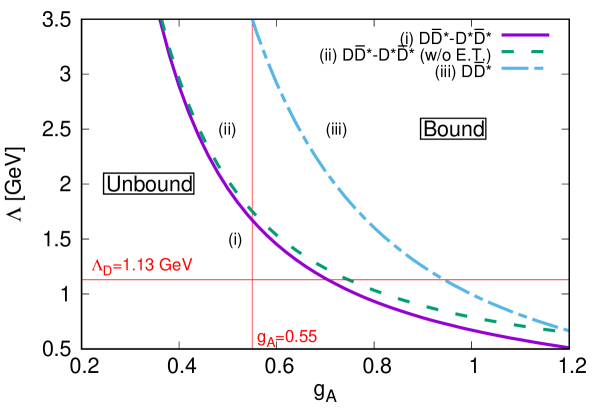
Figure 7: Boundary lines separating the regions where a bound state exists or not. The solid (i) and long-dashed (ii) lines are the results with and without the energy transfer, respectively. The dot-dashed line (iii) is the result without the $D^{(\ast)}\bar{D}^{(\ast)}$ channel (see the text for details). The right sides of these lines (i), (ii) and (iii) are the region where the system is bound in the cases of (i), (ii) and (iii), respectively, while the left side is the region where the the system is unbound. The vertical and horizontal solid lines shows the values at $g_{A}=0.55$ and at $\Lambda=\Lambda_{D}=1.13$ GeV, respectively.

The central and tensor potentials $C(r;m,\Lambda)$ and $T(r;m,\Lambda)$ for the $X(3872)$ in (182) are shown in figure 8, where the potentials with various effective pion masses are compared, $m=m_{\pi},0,\mu$. The potential with $m=m_{\pi}$ corresponds to the $D^{\ast}\bar{D}^{\ast}$ potential and the $D\bar{D}^{\ast}$ one in the static approximation, where the energy transfer is ignored. The potential with $m=\mu$ is the $D\bar{D}^{\ast}$ potential ${\cal C}_{\pi}$ taking into account the energy transfer. In figure 8 we plot only the real part of the potential. We also show the potential with $m=0$, which is in the limit of the small mass of the transfer pion. Since the central potential is proportional to the effective mass of the transfer pion, $m^{2}$, for $m^{2}=m^{2}_{\pi}>0$ in the static approximation, the overall sign of the potential $C(r;m_{\pi},\Lambda)$ is positive, while for $m^{2}=\mu^{2}<0$ with the energy transfer, the sign of the potential $C(r;\mu,\Lambda)$ is negative. The central potential vanishes for $m=0$. On the other hand, the tensor force does not depend on the effective pion mass strongly as shown in figure 8.

Naively, one would expect that a longer range potential yields more interaction strength, which we do not see here. One reason is that the central force has the factor $m^{2}$ as discussed. Another reason is that the tensor force is mostly effective at shorter distances than $1/m$, due to the $S$-$D$ coupling. In momentum space, it is due to the $\bi q^{2}$ dependence in the numerator (81) which increases the tensor force for large $\bi q^{2}$.

Central	Tensor

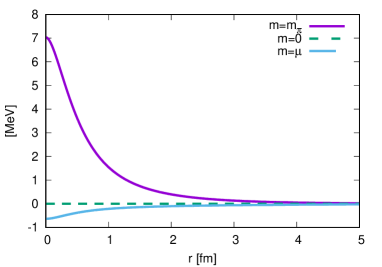
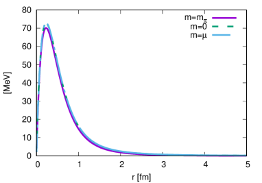
Figure 8: The central and tensor components of the OPEP for the $X(3872)$ (182), $\left(\frac{g_{A}}{2f_{\pi}}\right)^{2}C(r;m,\Lambda)$ and $\left(\frac{g_{A}}{2f_{\pi}}\right)^{2}T(r;m,\Lambda)$ respectively, with various effective pion masses and $(g_{A},\Lambda)=(0.55,1.13\,{\rm GeV})$. The solid, dashed and dashed-dot lines correspond to the potentials with $m=m_{\pi}(=137),0,\mu(=37.3i)$ MeV, respectively.

Turning to figure 7, the line (iii) shows the result without the $D^{\ast}\bar{D}^{\ast}$ channel. This line is far above the lines (i) and (ii), indicating that the attraction is significantly reduced. Since the coupling to $D^{\ast}\bar{D}^{\ast}$ component with the $D$-wave induces the tensor force as shown in (182), ignoring this component decreases the attraction due to the tensor force significantly. Hence, the full-coupled channel analysis of $D\bar{D}^{\ast}$ and $D^{\ast}\bar{D}^{\ast}$ is important when the tensor force of the OPEP is considered.

Figure 9: The boundaries of the $D^{(\ast)}\bar{D}^{(\ast)}$ (solid line) and $B^{(\ast)}\bar{B}^{(\ast)}$ (dashed double-dotted line) bound states in the $(g_{A},\Lambda)$ plane. The boundary of the $D^{(\ast)}\bar{D}^{(\ast)}$ state is the same as the boundary (i) in figure 7. The vertical solid line shows the value of $g_{A}=0.55$, and the horizontal solid and dashed lines show the values of $\Lambda=\Lambda_{D}=1.13$ GeV and $\Lambda=\Lambda_{B}=1.08$ GeV, respectively.

Finally, the $B^{(\ast)}\bar{B}^{(\ast)}$ bound state in the bottom sector is studied. We employ the same potential as used in the $D^{(\ast)}\bar{D}^{(\ast)}$ system (182) because the potential is given as the leading term of the $1/M_{P}$ expansion and thus the potential form is heavy flavor independent in the heavy quark limit. The cutoff $\Lambda_{B}$ for the $B$ meson is also evaluated by the hadron size in the similar way to the cutoff $\Lambda_{D}$. In [55], the ratio of the hadron size is obtained by $r_{N}/r_{B}=1.29$, and thus the cutoff $\Lambda_{B}$ is obtained by $\Lambda_{B}=1.29\Lambda_{N}=1.08$ GeV. This value can be the reference point here, while we also vary the cutoff to see the cutoff dependence. The use of different $\Lambda$ for charm and bottom sectors is to take partly into account $1/$(heavy quark mass) corrections due to kinematics, because in the quark model meson size is a function of the reduced mass.

In figure 9, the boundary line of the $B^{(\ast)}\bar{B}^{(\ast)}$ bound state is shown, where it is compared with the boundary of the $D^{(\ast)}\bar{D}^{(\ast)}$ bound state, which is the same as shown in figure 7 (i). The bound region for the $B^{(\ast)}\bar{B}^{(\ast)}$ system is larger than that of the $D^{(\ast)}\bar{D}^{(\ast)}$. In the bottom sector, the kinetic term is suppressed by the large $B^{(\ast)}$ meson mass, about 5 GeV, while the $D^{(\ast)}$ meson mass is about 2 GeV. In addition, the small mass difference between $B$ and $B^{\ast}$, about 46 MeV, magnifies the mixing rate of the $S$-$D$ coupled channel due to the tensor force, yielding more attraction. For the parameters $(g_{A},\Lambda)=(0.55,1.08\,{\rm GeV})$, the bound state is found in the bottom sector, where the binding energy is 6.3 MeV.

Because of the attraction in the bottom sector, the bottom counter part of the $X(3872)$ is also expected to be formed as the $B^{(\ast)}\bar{B}^{(\ast)}$ bound state. Verification in experiments is needed.

4.3 Admixture of the $c\bar{c}$ core and the $D\bar{D}^{*}$ molecule

As discussed in the previous section, the OPEP tensor term induces the $D^{(*)}\bar{D}{}^{(*)}$ $S$-$D$-wave channel mixing, which gives an attraction to the $X$(3872) system. This attraction is sizable, but seems not large enough to produce a bound state. Another origin of the attraction is discussed in [115], where $X$(3872) is assumed to be a shallow bound state of the coupled channels of $c\bar{{c}}$, ${D^{0}\bar{{D}}{}^{*0}}$ and the ${D^{+}D^{*-}}$. The coupling occurs between the bare $c\bar{c}$ pole and the isospin-0 $S$-wave $D\bar{{D}}{}^{*}$ continuum. A nearby $c\bar{{c}}(1^{++})$ state is $\chi_{c1}(2P)$, which has not been observed experimentally but was predicted by the quark model [181]. The predicted mass of $\chi_{c1}(2P)$ is by about 80 MeV above the $D\bar{{D}}{}^{*}$ threshold energy according to the quark model. So, the coupling to the $c\bar{{c}}$ state pushes the low energy $D\bar{{D}}{}^{*}$ continuum states downward, toward the threshold. As a result, the coupling provides an attraction for the isospin-0 $S$-wave $D\bar{{D}}{}^{*}$. This dynamically generates a pole, $X$(3872), while the $c\bar{c}$ state gets a broad width, which makes the state difficult to observe.

The $c\bar{{c}}$-$D\bar{D}{}^{*}$ coupling occurs in the short range where the light quark pair in the $D\bar{{D}}{}^{*}$ state can annihilate. On the other hand, the size of $X$(3872) is very large as shown later in table 8. The volume of the interaction region is the order of $10^{-3}$ of that of the $X$(3872) [182]. Since most of the $X$(3872) wave function stays spatially outsize of the interaction region, one may wonder whether such a short range coupling can be responsible to make the $X$(3872). Actually, any potential of a finite range can make a bound state with an appropriate strength. Suppose we employ a three-dimensional square-well potential of the range $a$ and the strength $V_{0}$. Then one bound state at the threshold appears when $V_{0}\sim\pi^{2}/(8\mu a^{2})$. Since the reduced mass of the $D\bar{D}^{*}$ system is about 1 GeV, the required strength $V_{0}$ to make a bound state is 50–200 MeV for $a\sim$ 0.5–1 fm. This size of the strength is reasonable when considering that the typical mass difference of the hadrons, such as $D^{*}$-$D$ (140 MeV) or as $J/\psi$-$\eta_{c}$ (113 MeV), is the order of 100 MeV. So, in this section, we study $X$(3872) in a coupled channel model of $c\bar{{c}}$, $D^{(*)0}\bar{{D}}{}^{(*)0}$ and $D^{(*)+}D^{(*)-}$.

To start with, we investigate a simple model of such, a model of coupled channels of $D\bar{D}^{*}$ and $c\bar{c}$ where the interaction of $D\bar{D}^{*}$ takes place only through their coupling to $c\bar{c}$ channel. We call this $c\bar{c}$ model, where, in the absence of OPEP, only the $S$-waves are relevant for $D\bar{D}^{*}$ channels. It is reported that by assuming a coupling between $c\bar{c}$ and ${D^{0}\bar{{D}}{}^{*0}}$ and ${D^{+}D^{*-}}$, a shallow bound state appears below the ${D^{0}\bar{{D}}{}^{*0}}$ threshold; but there is no peak structure found at the ${D^{+}D^{*-}}$ threshold. The coupling structure is assumed as

$$\langle{D^{+}D^{*-}}({\bi q})|U|c\bar{c}\rangle=-\langle{D^{0}\bar{{D}}{}^{*0}}({\bi q})|U|c\bar{c}\rangle={g_{c\bar{c}}\over\sqrt{\Lambda_{q}}}{\Lambda_{q}^{2}\over q^{2}+\Lambda_{q}^{2}}.$$ (188)

The coupling strength $g_{c\bar{c}}$ is taken so as to produce the observed mass of $X$(3872). The cutoff $\Lambda_{q}$ is roughly corresponds to the inverse of the size of the region where the $q\bar{q}$ annihilation occurs, being $U\propto e^{-\Lambda_{q}r}/r$. Here we show the results with $\Lambda_{q}$ = 0.5 GeV $\sim$ (0.4 fm)^-1 [115]. When one uses smaller value for $\Lambda_{q}$, e.g. 0.3 GeV, the model gives a sizable enhancement around the mass of $\chi_{c1}(2P)$, 3950 MeV, in the final $D\bar{{D}}^{*}$ mass spectrum of the $B\to D\bar{{D}}^{*}K$ decay. Since such a structure is not observed, it can be a constraint to the interaction region from the $B$-decay experiments that $\Lambda_{q}$ is more than about 0.5 GeV [115].

The mass of the charged $D$ meson is heavier than the neutral one by 4.822$\pm$0.015 MeV and that of $D^{*}$ by 3.41$\pm$0.07 MeV [5]. Therefore, the threshold difference between ${D^{0}\bar{{D}}{}^{*0}}$ and ${D^{+}D^{*-}}$ is about 8.2 MeV. Since the $X(3872)$ mass is almost at the ${D^{0}\bar{{D}}{}^{*0}}$ threshold, the major component of the $X(3872)$ is considered to be ${D^{0}\bar{{D}}{}^{*0}}$. In such a situation, it is convenient to look into $X$(3872) in the particle basis rather than in the isospin basis. The wave functions of the $S$-wave $D\bar{{D}}{}^{*}$ components of the $X$(3872) obtained by using the $c\bar{c}$ model are plotted by the long dashed curves in figure 10. In the $c\bar{c}$ model only the S-waves are relevant. The ${D^{0}\bar{{D}}{}^{*0}}$ wave function is actually large in size and has a very long tail. Its root mean square distance (rms) is listed in table 8. Note that this number varies rapidly as the binding energy varies because the rms becomes infinite as the binding energy goes zero as seen from (90). The rms of the ${D^{+}D^{*-}}$ component is much smaller than that of the ${D^{0}\bar{{D}}{}^{*0}}$ because of the ${D^{0}\bar{{D}}{}^{*0}}$-${D^{+}D^{*-}}$ threshold difference. As seen from figure 10, the amplitudes of the ${D^{0}\bar{{D}}{}^{*0}}$ and the ${D^{+}D^{*-}}$ wave functions are similar in size in the very short range region where the $D\bar{{D}}{}^{*}$ state couples to the $c\bar{{c}}$; the isospin-0 $D\bar{{D}}{}^{*}$ state becomes a dominant component there as shown in figure 11. Probabilities of various components of the bound state are shown in the first line of table 9. As was mentioned in section 6, the production rate of $X$(3872) in the $p\bar{p}$ collision experiments suggests that the amount of the $c\bar{c}$ component is expected to be several %. In the present $c\bar{c}$ model, the admixture is 8.6%. As we will show later, by introducing OPEP between the $D$ and $\bar{{D}}$ mesons, this admixture reduces to 5.9 %, which corresponds to the amount just required from the experiments.

Table 8: Parameters and the root mean square distance (rms) of the two mesons in $X$(3872) in the $c\bar{c}$ model ($c\bar{c}$) [115], in the OPEP model (OPEP) [183], and in the $c\bar{c}$-OPEP model ($c\bar{c}$-OPEP) [183]. The rms₀ (rms_±) means the rms between $D^{(*)0}$ and $\bar{D}{}^{(*)0}$ ($D^{(*)+}$ and $D{}^{(*)-}$). BE is the binding energy in MeV. (90) stands for the values calculated by using (90).

	$g_{c\bar{c}}$	$\Lambda_{q}$ (GeV)	$g_{A}$	$\Lambda$ (GeV)	rms0 (fm)	rms± (fm)	BE(MeV)
$c\bar{c}$	0.05110	0.5	-	-	8.39	1.56	0.16
OPEP	-	-	0.55	1.791	8.25	1.44	0.16
$c\bar{c}$-OPEP	0.04445	0.5	0.55	1.13	8.36	1.59	0.16
(90)	-	-	-	-	7.93	1.11	0.16

Table 9: Probabilities of each components of $X$(3872) in the $c\bar{c}$ model ($c\bar{c}$) [115], in the OPEP model (OPEP) [183], and in the $c\bar{c}$-OPEP model ($c\bar{c}$-OPEP) [183]. $|c_{c\bar{c}}|^{2}$ stands for the probability of the $c\bar{{c}}$ component, $|c_{0,\pm}({{}^{3}\!S})|^{2}$ stands for the ${D^{0}\bar{{D}}{}^{*0}}$ (${D^{+}D^{*-}}$) $({}^{3}\!S)$ component, $|c_{0,\pm}({{}^{2S+1}\!D})|^{2}$ for the ${D^{0}\bar{{D}}{}^{*0}}$ (${D^{+}D^{*-}}$) $({}^{2S+1}\!D)$ component. $D$ stands for the $D$-state probabilities, $\sum|c_{0,\pm}(^{2S+1}D)|^{2}$.

model	$|c_{c\bar{c}}|^{2}$	$|c_{0}({{}^{3}\!S})|^{2}$	$|c_{0}({{}^{3}\!D})|^{2}$	$|c_{0}({{}^{5}\!D})|^{2}$	$|c_{\pm}({{}^{3}\!S})|^{2}$	$|c_{\pm}({{}^{3}\!D})|^{2}$	$|c_{\pm}({{}^{5}\!D})|^{2}$	$D$(%)
$c\bar{c}$	0.086	0.848	-	-	0.067	-	-	-
OPEP	-	0.910	0.004	0.004	0.073	0.005	0.006	2.0
$c\bar{c}$-OPEP	0.059	0.869	0.002	0.001	0.065	0.002	0.001	0.6

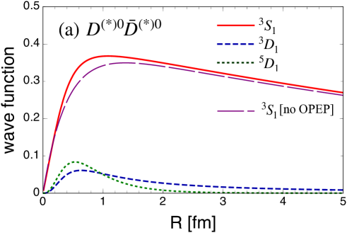
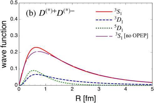
Figure 10: (a) The ${D^{0}\bar{{D}}{}^{*0}}$ and (b) the ${D^{+}D^{*-}}$ wave function of $X$(3872) in the OPEP model; solid lines are for $D\bar{{D}}{}^{*}({}^{3}S_{1})$, dashed lines for $({}^{3}D_{1})$ and dotted lines for $D^{*}\bar{{D}}{}^{*}({}^{5}D_{1})$. The long dashed lines are for those of [115], which corresponds the $c\bar{c}$-model in tables 8 and 9, where the $X$(3872) consists of the $c\bar{{c}}$ and the $D\bar{{D}}{}^{*}({}^{3}S_{1})$ components, without OPEP. The sign of the wave functions is taken to be positive at small $r$.

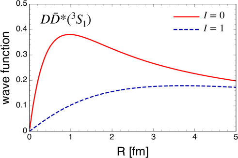
Figure 11: The $D\bar{{D}}{}^{*}$ wave function of $X$(3872) in the isospin basis. The solid (dashed) line is for the isospin 0 (1) wave function of the $c\bar{c}$ model. The sign of the wave functions is taken to be positive at small $r$.

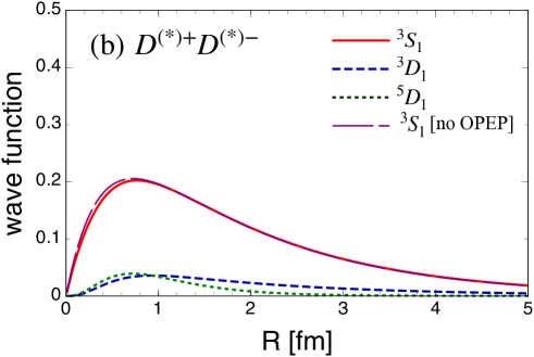
Figure 12: (a) The ${D^{0}\bar{{D}}{}^{*0}}$ and (b) the ${D^{+}D^{*-}}$ wave function of $X$(3872) in the $c\bar{c}$-OPEP model with the same convention as in figure 10.

Now we consider models with OPEP included; the one denoted as OPEP in table 9 is the model with only the $D^{(*)}\bar{D}^{(*)}$ channels included as discussed in section 4.2, and the other one denoted as $c\bar{c}$-OPEP is the $c\bar{c}$-$D^{(*)}\bar{D}^{(*)}$ coupled channel model with the OPEP and their $S$-$D$ tensor couplings included [183]. The model space is now taken to be ${c\bar{c}}$, $D^{(*)0}\bar{{D}}{}^{(*)0}$ and $D^{(*)+}D^{(*)-}$ found in (178):

$$\Psi = c_{c\bar{c}}|c\bar{{c}}\rangle+\psi_{0}+\psi_{\pm},$$ (189)

$$\psi_{0,\pm} = c_{0,\pm}({}^{3}\!S)|D\bar{{D}}{}^{*}({}^{3}\!S_{1})\rangle+c_{0,\pm}({}^{3}\!D)|D\bar{{D}}{}^{*}({}^{3}\!D_{1})\rangle+c_{0,\pm}({}^{5}\!D)|D^{*}\bar{{D}}{}^{*}({}^{5}\!D_{1})\rangle,$$

where $c_{c\bar{c}}$ is the amplitude of the $c\bar{c}$ component, $c_{0}({}^{3}\!S)$ is that of the ${D^{0}\bar{{D}}{}^{*0}}({}^{3}\!S_{1})$ component, $c_{\pm}({}^{3}\!S)$ is that of the ${D^{+}D^{*-}}({}^{3}\!S_{1})$ component, and so on.

The OPEP potential among the $I(J^{PC})=0(1^{++})$ $D^{(*)}\bar{{D}}{}^{(*)}$ states are found in (182). In the particle base calculation, it is convenient to use the expression with the explicitly written isospin factor

$$V_{\pi}(r) = -\left(\frac{g_{A}}{2f_{\pi}}\right)^{2}\frac{1}{3}\left(\begin{array}[]{ccc}{\cal C}_{\pi}&-\sqrt{2}{\cal T}_{\pi}&-\sqrt{6}T_{\pi}\\ -\sqrt{2}{\cal T}_{\pi}&{\cal C}_{\pi}+{\cal T}_{\pi}&-\sqrt{3}T_{\pi}\\ -\sqrt{6}T_{\pi}&-\sqrt{3}T_{\pi}&C_{\pi}-T_{\pi}\\ \end{array}\right)\boldsymbol{\tau}_{1}\cdot\boldsymbol{\tau}_{2},$$ (194)

where $C_{\pi}$, $T_{\pi}$, ${\cal C}_{\pi}$, and ${\cal T}_{\pi}$ are the same as those defined for (182). The $c\bar{c}$-$D\bar{{D}}{}^{*}$ coupling is taken as (188). The parameters are listed in table 8. The OPEP cutoff $\Lambda$ in the OPEP-model is taken to be a free parameter to reproduce a bound state with the binding energy, 0.16 MeV. As for the $c\bar{c}$-OPEP model, the OPEP cutoff $\Lambda=\Lambda_{D}$ is the standard one obtained from the $D$-meson size as marked in figure 7 in the previous subsection. The $c\bar{c}$-$D\bar{{D}}$ coupling strength, $g_{c\bar{c}}$, in the $c\bar{c}$-OPEP model is taken to be a free parameter to fit the binding energy.

In table 8, rms of the ${D^{0}\bar{{D}}{}^{*0}}$ and ${D^{+}D^{*-}}$ system are listed. The size of $X$(3872), governed mostly by the binding energy, does not depend much on details of the model. The wave functions of each model are plotted in figure 10 and figure 12. The $D\bar{{D}}{}^{*}$ ${}^{3}S_{1}$ wave functions are similar to each other, though they are slightly enhanced at the short distance in the OPEP model. This is due to the tensor force; the $S$-$D$ coupling causes effectively an attraction in the $S$-wave channel which contains the square of the $D$-wave amplitude. In fact, the location of the maximum strength of the $D$-wave amplitude roughly coincides with where the ${}^{3}S_{1}$ wave function is enhanced.

In the $c\bar{c}$ model, the attraction comes from the $c\bar{c}$-$D\bar{{D}}^{*}$ coupling, while the $S$-$D$-wave mixing by the OPEP tensor term provides the attraction in the OPEP model. Their effects can be roughly estimated by the amounts of the ${c\bar{c}}$ components, $|c_{c\bar{c}}|^{2}$, and the $D$-state probabilities, which are listed in table 9. In the ${c\bar{c}}$-OPEP model, where both of these attractions are introduced, $|c_{c\bar{c}}|^{2}$ reduces from 8.6 % to 5.9 %, while the $D$-state probabilities reduces from 2.0 % to 0.6 %. The former reduces to 2/3, and the latter reduces to 1/3, which are the rough share of the attraction in the $c\bar{c}$-$D\bar{{D}}^{*}$ coupling model with a reasonable cutoff for the OPEP. The $D$-state probability and the $c\bar{{c}}$ probability depend much on the binding energy, or on slight change of $g_{A}$, whose value is determined in the heavy quark limit. The size of the $c\bar{c}$ component can also vary as shown in the next subsection. Therefore, it is difficult to estimate the relative importance of OPEP quantitatively. Qualitatively, however, we can conclude that effects of the $c\bar{c}$-$D\bar{{D}}{}^{*}$ coupling and OPEP are comparable in $X$(3872). One has to consider the coupled channel system of the $c\bar{{c}}$ pole, the ${D^{0}\bar{{D}}{}^{*0}}$ and the ${D^{+}D^{*-}}$ scattering channels with their mass difference, and the $c\bar{c}$-$D\bar{{D}}^{*}$ coupling and the OPEP, simultaneously, to understand the feature of $X$(3872).

4.4 The decay spectrum of $X(3872)$

The strong decay modes of $X(3872)$ observed up to now are $J\!/\!\psi\pi^{+}\pi^{-}$, $J\!/\!\psi\pi^{+}\pi^{-}\pi^{0}$, $D^{0}\bar{{D}}{}^{*0}$[5], and recently, $\chi_{c1}\pi^{0}$ [130]. Here we discuss the strong decay of $X(3872)$, especially the following two notable features to understand the $X$(3872) nature. One is that a large isospin symmetry breaking is found in the final decay fractions: as seen in (176), the decay fractions of $X$(3872) going into $J\!/\!\psi\pi^{3}$ and $J\!/\!\psi\pi^{2}$ indicate that amounts of the $J\!/\!\psi\omega$ and $J\!/\!\psi\rho^{0}$ components in $X$(3872) are comparable to each other as shown in (177). The other feature we would like to discuss here is that the decay width of the $X$(3872) is very small for a resonance above the open charm threshold, or for a resonance decaying through the $\rho$ and $\omega$ components, which themselves have a large decay width.

In the following we employ a model which consists of the $c\bar{c}$ core, ${D^{0}\bar{{D}}{}^{*0}}$, ${D^{+}D^{*-}}$, $J\!/\!\psi\omega$ and $J\!/\!\psi\rho^{0}$. The system here does not include the $\chi_{c1}\pi^{0}$ channel. Since an amount of the observed fraction is about the same as that of the $J\!/\!\psi\rho^{0}$, this channel can probably be treated by a perturbational; properties of the other channels will not change much if this $\chi_{c1}\pi^{0}$ channel is introduced. Moreover, since its threshold is lower than the $X$(3872) by 230 MeV, it will be necessary to consider the pion radiation from the $D^{(*)}\bar{D}{}^{(*)}$ components to obtain the $\chi_{c1}\pi^{0}$ fraction. Here the model contains only the relative $S$-wave hadron systems which have thresholds close to each other.

For the discussions of decay properties here, it is sufficient to consider the formation of a loosely bound $D\bar{D}^{*}$ states, which couple to the $c\bar{c}$ and to the $J\psi\rho$ and $J\psi\omega$ with finite decay widths for $\rho$ and $\omega$. We assume effective couplings between $c\bar{c}$ and $D\bar{{D}}{}^{*}$, which gives the attraction as we discussed in the previous section, and between $D\bar{{D}}{}^{*}$ and $J\!/\!\psi\omega(\rho^{0})$, which expresses the rearrangements. In this section we do not introduce OPEP; the system is restricted only to the $S$-waves, and the attraction from the OPEP is effectively taken into account by introducing the central attraction between the $D^{(*)}$ and $\bar{{D}}{}^{(*)}$. The widths of the $\omega$ and $\rho$ mesons are taken into account as an imaginary part in the $J/\psi\omega$ and $J/\psi\rho$ propagators. In this way, we consider that the model can simulate essential features of the decay properties of $X(3872)$.

From the quark model point of view, the $D\bar{{D}}{}^{*}$ states of total charge 0 are the $c\bar{{c}}u\bar{{u}}$ or $c\bar{{c}}d\bar{{d}}$ states, which contain also the $J\!/\!\psi\omega$ or $J\!/\!\psi\rho^{0}$ state with the appropriate color configuration. The observed final $J\!/\!\psi\pi^{3}$ and $J\!/\!\psi\pi^{2}$ decay modes are considered to come from these components. The rearrangement between $D\bar{{D}}{}^{*}$ and $\omega J\!/\!\psi$ or $\rho^{0}J\!/\!\psi$ occurs at the short distance, where all four quarks exist in the hadron size region. The coupling between the $c\bar{c}$ and $D\bar{D}{}^{*}$, however, is not known. Therefore, it is treated as a phenomenological one, as shown below. Note that there is no direct channel coupling between the $c\bar{{c}}$ channel and the $\omega J\!/\!\psi$ or $\rho^{0}J\!/\!\psi$ channels in the present model setup. They break the OZI rule, and the latter breaks the isospin symmetry.

The model Hamiltonian for the $c\bar{{c}}$, $D^{0}\bar{{D}}{}^{*0}$, $D^{+}D^{-*}$, $J\!/\!\psi\omega$ and $J\!/\!\psi\rho$ channels is taken as [38]:

$$H = \left(\begin{array}[]{ccccccc}m_{c\bar{c}}&U^{(mc)}{}^{\dagger}\\ U^{(mc)}&H^{(mm)}\\ \end{array}\right),$$ (197)

$$H^{(mm)} = H^{(mm)}_{0}+V^{(mm)},$$ (198)

$$H^{(mm)}_{0} = {\rm diag}(K_{D{\bar{D}}0},K_{D{\bar{D}}\pm},K_{J/\psi\omega},K_{J/\psi\rho}),$$ (199)

$$K_{D{\bar{D}}0,\pm} = m_{D^{0,-}}+m_{D^{*0,+}}+{p^{2}\over 2\mu_{D{\bar{D}}0,\pm}},$$ (200)

$$K_{J\!/\!\psi\omega,\rho} = m_{J\!/\!\psi}+m_{\omega,\rho}+{p^{2}\over 2\mu_{J/\psi\omega,\rho}},$$ (201)

$$U^{(mc)} = \left(\begin{array}[]{ccccccc}-u\\ u\\ 0\\ 0\\ \end{array}\right),~{}~{}~{}V^{(mm)}=\left(\begin{array}[]{ccccccc}\tilde{v}&0&-v&-v\\ 0&\tilde{v}&v&-v\\ -v&v&0&0\\ -v&-v&0&0\\ \end{array}\right),$$ (210)

$$u(q) = {g_{c\bar{c}}\over\sqrt{\Lambda_{q}}}L_{\Lambda_{q}}(q),~{}~{}~{}~{}L_{\Lambda_{q}}(q)={\Lambda_{q}^{2}\over\Lambda_{q}^{2}+q^{2}},$$ (211)

$$v(q,q^{\prime}) = {v_{0}\over\Lambda_{q}^{2}}L_{\Lambda_{q}}(q)L_{\Lambda_{q}}(q^{\prime}),~{}~{}~{}\tilde{v}(q,q^{\prime})={\tilde{v}_{0}\over\Lambda_{q}^{2}}L_{\Lambda_{q}}(q)L_{\Lambda_{q}}(q^{\prime}),$$ (212)

where $m_{c\bar{c}}$ is the $c\bar{{c}}$ bare mass when the coupling to $D\bar{{D}}{}^{*}$ is switched off. The reduced masses, $\mu_{D{\bar{D}}0,\pm}$ and $\mu_{J/\psi\omega,\rho}$, are for the $D{}^{0}\bar{{D}}{}^{*0}$, $D^{\pm}D^{*\mp}$, $J\!/\!\psi\omega$ and $J\!/\!\psi\rho$ systems, respectively. The coupling between the $c\bar{{c}}$ state and the $D\bar{{D}}{}^{*}$ state is expressed by the transfer potential, $U^{(mc)}$, which is chosen to be Lorentzian in the momentum space with the strength $g_{c\bar{c}}$. The rearrangement between the $D\bar{{D}}{}^{*}$ states and the $J\!/\!\psi\omega$ and $J\!/\!\psi\rho$ meson is expressed by a separable potential, $v$ in $V^{(mm)}$. The basis of the matrix expression in (199) and in (210) are ($D^{(*)0}\bar{{D}}{}^{(*)0}$, $D^{(*)\pm}D^{(*)\mp}$, $J\!/\!\psi\omega$, $J\!/\!\psi\rho^{0}$). The strength of the interaction between the $D$ and $\bar{{D}}$ mesons, $\tilde{v}_{0}$, is taken to be the maximal value which does not create a bound state in the $B\bar{B}$ systems, where no bound states has been observed yet. The strengths $g_{c\bar{c}}$ and $v_{0}$ are free parameters under the condition that the mass of $X$(3872) can be reproduced. The value of $\Lambda_{q}$ is the same as the one used in the previous section, $\Lambda_{q}$ = 0.5 GeV. The parameters are summarized in table 10.

Table 10: Model parameters and the amounts of each component. Masses and widths are in MeV, and taken from [184]

$m_{J/\psi}$	$m_{\omega}$	$\Gamma_{\omega}$	$m_{\rho}$	$\Gamma_{\rho}$	$g_{c\bar{c}}$	$v_{0}$	$\tilde{v}_{0}$
3096.916	782.65	8.49	775.26	147.8	0.04136	0.1929	$-0.1886$
$|c_{c\bar{c}}|^{2}$	$|c_{0}(^{3}S)|^{2}$	$|c_{\pm}(^{3}S)|^{2}$	$|c_{J/\psi\omega}|^{2}$	$|c_{J/\psi\rho}|^{2}$
0.036	0.913	0.034	0.010	0.006

The amount of each component in the $X$(3872) bound state is also listed in table 10. The bulk feature is similar to the models in the previous section: the dominant component is ${D^{0}\bar{{D}}{}^{*0}}$ while the ${D^{+}D^{*-}}$ component is considerably smaller because of the threshold difference. The amount of the $c\bar{c}$ component is somewhat smaller but still sizable. The $J/\psi\omega$ and $J/\psi\rho$ components are small comparing to the $D\bar{{D}}{}^{*}$ components. The fact that the $J/\psi\rho$ and $J/\psi\omega$ components of $X$(3872) are comparable in size is reproduced in the present model.

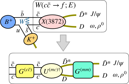
Figure 13: The $B$ meson weak decay. See text.

As listed in table 6, the $X$(3872) is produced by various processes. As a typical example, we discuss the $X$(3872) decay process in the $B$ meson weak decay in the following. As illustrated in figure 13, the mass spectrum of $X$(3872) from the $B$ meson weak decay is proportional to the sum of the transfer strength from the $c\bar{{c}}$ to the two-meson states, $f$, $W(c\bar{{c}}\rightarrow f;E)$, which can be expressed as

$$\sum_{f}{\rmd W(c\bar{{c}}\rightarrow f;E)\over\rmd E}=-{1\over\pi}{\rm Im}\langle c\bar{{c}}|{G^{(c\bar{c})}}(E)|c\bar{{c}}\rangle.$$ (213)

Here ${G^{(c\bar{c})}}$ is the full propagator of the $c\bar{{c}}$ state, which can be written by using the self energy $\Sigma_{c\bar{c}}$ as:

$${G^{(c\bar{c})}}(E) = (E-m_{c\bar{c}}-\Sigma_{c\bar{c}}(E))^{-1},$$ (214)

$$\Sigma_{c\bar{c}}(E) = U^{(mc)}{}^{\dagger}{G^{(mm)}}(E)U^{(mc)}.$$ (215)

Here we define the free and the full propagators within the two-meson space, ${G^{(mm)}_{0}}(E)$ and ${G^{(mm)}}(E)$, respectively, with the decay widths as

$${G^{(mm)}_{0}}(E) = \Big{(}E-H_{0}^{(mm)}+\rmi{\Gamma\over 2}\Big{)}^{-1},$$ (216)

$${G^{(mm)}}(E) = \Big{(}E-H^{(mm)}+\rmi{\Gamma\over 2}\Big{)}^{-1},$$ (217)

$$\Gamma = {\rm diag}(0,0,\Gamma_{\omega},\Gamma_{\rho}),$$ (218)

where $\Gamma_{\omega,\rho}$ is the $\omega$ or $\rho$ decay width, respectively. The $\rho$ meson width is taken to be energy dependent as discussed in [38]. The widths of $D^{*}$ mesons are neglected. The width $\Gamma$ is ignored when the bound state energy or the component is calculated above. It, however, is essential to include them when one investigates the decay spectrum.

In order to obtain the decay spectrum of each final two-meson channel separately, we have rewritten the right-hand side of (213) as follows. Since the system has only one $c\bar{c}$ state in the present model, the above ${G^{(c\bar{c})}}(E)$ and $\Sigma_{c\bar{c}}(E)$ are single channel functions of the energy $E$. They become matrices when more than one $c\bar{c}$ states are introduced, but the following procedure can be extended in a straightforward way. As seen from (214), the imaginary part of ${G^{(c\bar{c})}}(E)$ comes only from the imaginary part of $\Sigma_{c\bar{c}}(E)$. Therefore,

$${\rm Im}\,{G^{(c\bar{c})}} = {\rm Im}\,({G^{(c\bar{c})}}^{*}\,({G^{(c\bar{c})}}^{*})^{-1}\,{G^{(c\bar{c})}})={\rm Im}\,({G^{(c\bar{c})}}^{*}\,\Sigma_{c\bar{c}}\,{G^{(c\bar{c})}})$$ (219)

$$= {\rm Im}\,({G^{(c\bar{c})}}^{*}\,U^{(mc)}{}^{\dagger}{G^{(mm)}}U^{(mc)}\,{G^{(c\bar{c})}}),$$

where ^∗ stands for the complex conjugate. Using the following relation for a real potential

$${\rm Im}\,{G^{(mm)}}^{-1} = {\rm Im}\,{G^{(mm)}_{0}}^{-1}$$ (220)

and Lippmann Schwinger equation for the propagator, $G=(1+GV)G_{0}$, we have for Im${G^{(mm)}}$ on the right-hand side of (219)

$${\rm Im}\,{G^{(mm)}} = {\rm Im}\,({G^{(mm)}}({G^{(mm)}}{}^{*})^{-1}{G^{(mm)}}{}^{*})$$ (221)

$$= {\rm Im}\,({G^{(mm)}}({G^{(mm)}_{0}}{}^{*})^{-1}{G^{(mm)}}{}^{*})$$

$$= {\rm Im}\,\Big{(}(1+{G^{(mm)}}V^{(mm)}){G^{(mm)}_{0}}(1+{G^{(mm)}}{}^{*}V^{(mm)})\Big{)}.$$

Thus, (219) can be rewritten as

$${\rm Im}\,{G^{(c\bar{c})}} = {\rm Im}\,\Big{(}{G^{(c\bar{c})}}^{*}U^{(mc)}{}^{\dagger}(1+{G^{(mm)}}V^{(mm)}){G^{(mm)}_{0}}(1+{G^{(mm)}}{}^{*}V^{(mm)})U^{(mc)}{G^{(c\bar{c})}}\Big{)}.$$

When we apply the plain wave expansion for the ${G^{(mm)}_{0}}$ in (LABEL:eq:ImG-3), we have

$${\rmd W(c\bar{{c}}\rightarrow f;E)\over\rmd E}$$

$$= -{1\over\pi}{\rm Im}\int{\rm d}{\bi k}\langle f{\bi k}|{G^{(mm)}_{0}}(E)|f{\bi k}\rangle\Big{|}\sum_{f^{\prime}}\int\rmd{{\bi k}^{\prime}}\langle\!\langle f^{\prime}{\bi k}^{\prime}(f{\bi k})|U^{(mc)}({\bi k}^{\prime}){G^{(c\bar{c})}}(E)|c\bar{c}\rangle\Big{|}^{2}$$

$$= {2\over\pi}\mu_{f}\int{k^{2}{\rm d}k\;\mu_{f}\Gamma_{f}\over(k_{f}^{2}-k^{2})^{2}+(\mu_{f}\Gamma_{f})^{2}}\Big{|}\sum_{f^{\prime}}\int\rmd{{\bi k}^{\prime}}\langle\!\langle f^{\prime}{\bi k}^{\prime}(f{\bi k})|U^{(mc)}({\bi k}^{\prime}){G^{(c\bar{c})}}(E)|c\bar{c}\rangle\Big{|}^{2},$$

where $k_{f}$ and $\mu_{f}$ stand for the three-momentum and the reduced mass of the final two-meson state where $E=m_{1f}+m_{2f}+k_{f}^{2}/(2\mu_{f})$. $\Gamma_{f}$ is the the decay width of mesons in the final state $f$, i.e. 0 if $f$ is $D\bar{{D}}{}^{*}$, $\Gamma_{\omega}$ or $\Gamma_{\rho}$ when $f$ is $J/\psi\omega$ or $J/\psi\rho$. $|f{\bi k}\rangle$ stands for the plain wave of the channel $f$ with the momentum ${\bi k}$. $|f^{\prime}{\bi k}^{\prime}(f{\bi k})\rangle\!\rangle$ stands for the distorted wave function of the channel $f^{\prime}$ with the momentum ${\bi k}^{\prime}$ which is generated from $|f{\bi k}\rangle$. This can be obtained by the Lippmann Schwinger equation as

$$|f^{\prime}{\bi k}^{\prime}(f{\bi k})\rangle\!\rangle = (1+{G^{(mm)}}V^{(mm)})|f{\bi k}\rangle.$$ (224)

In the present model, only the $D\bar{D}{}^{*}$ channels couple directly to $c\bar{c}$. The summation over $f^{\prime}$ in (LABEL:eq:X3872-width) means summation over $D^{0}\bar{{D}}{}^{*0}$ and $D^{+}D^{-*}$. The final two-meson fraction expressed by $f$ in the above equations can be $J\!/\!\psi\omega$ or $J\!/\!\psi\rho$ as well as $D\bar{D}{}^{*}$. For the channels where $\Gamma_{f}$ is small, the transfer strength becomes

$${\rmd W(c\bar{{c}}\rightarrow f;E)\over\rmd E} \rightarrow \mu_{f}k_{f}\Big{|}\sum_{f^{\prime}}\int\rmd{{\bi k}^{\prime}}\langle\!\langle f^{\prime}{\bi k}^{\prime}(fk_{f})|U^{(mc)}({\bi k}^{\prime}){G^{(c\bar{c})}}(E)|c\bar{c}\rangle\Big{|}^{2}~{}~{}~{}(\Gamma_{f}\rightarrow 0).$$

The calculated $W$ spectrum is shown for each final state in figure 14. The narrow peak at around the $D^{0}\bar{{D}}{}^{*0}$ threshold as well as the large isospin mixing are successfully reproduced by this picture of the $c\bar{{c}}$, $D^{0}\bar{{D}}{}^{*0}$, $D^{+}D^{-*}$, $J\!/\!\psi\omega$ and $J\!/\!\psi\rho$. The spectrum shape depends on the $X$(3872) binding energy, but the qualitative feature does not. The $J\!/\!\psi\omega$ and $J\!/\!\psi\rho$ peaks in the decay spectrum remain sharp when the $X$(3872) is around the threshold[38].

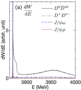
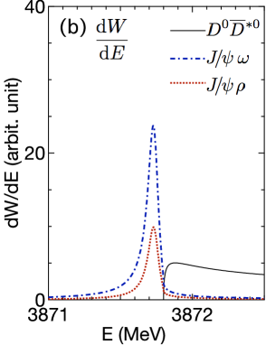
Figure 14: The transfer strength from the $c\bar{{c}}$ state to the final two-meson states. The energy $E$ is the center of mass energy of the two-meson states. Figure (b) is the same as (a) but magnified at around the $D^{0}\bar{{D}}{}^{*0}$ threshold. Taken from [38].

Let us discuss the mechanism to have the small width of the peak and the isospin mixing in the final fractions, the two notable features of the final $J\!/\!\psi\omega(\rho)$ spectrum mentioned before. The small width of $X$(3872) means that the corresponding pole of ${G^{(c\bar{c})}}$ is close to the real axis. The imaginary part in the denominator of ${G^{(c\bar{c})}}$ comes from the imaginary part of $\Sigma_{c\bar{c}}$ as shown (214), which can be expanded by using (215) as

$$\Sigma_{c\bar{c}} = u^{\dagger}G^{(D\bar{D}{}^{*})}u+u^{\dagger}G^{(D\bar{D}{}^{*})}vG^{(J/\psi\omega,\rho)}_{0}vG^{(D\bar{D}{}^{*})}u+\cdots,$$

$$= u^{\dagger}G^{(D\bar{D}{}^{*})}u\Big{(}1+{g_{c\bar{c}}}^{-1}v_{0}^{2}(\Lambda_{q}^{-2}L_{\Lambda_{q}}G^{(J/\psi\omega,\rho)}_{0}L_{\Lambda_{q}})(\Lambda_{q}^{-3/2}L_{\Lambda_{q}}G^{(D\bar{D}{}^{*})}u)+\cdots\Big{)},$$

where $G^{(D\bar{D}{}^{*})}$ stands for the full propagator obtained within the $D\bar{{D}}{}^{*}$ space, and the second equation can be obtained for the separable potential, (212) and (211).

On the right-hand side of (LABEL:eq:Sigcc-1), the first term is real for the energy below the threshold. It is because there is no bound state without the $c\bar{c}$ core, and also because the decay width of $D^{*}$ is very small, $83.4\pm 1.8$ keV for $D^{*\pm}$ and $<2.1$ MeV for $D^{*0}$ [5], and can be neglected. The first term gives most of the size of the real part of the self energy, $\Sigma_{c\bar{c}}$, which gives the mass difference between the $c\bar{c}$ core and the $X$(3872).

The second term has an imaginary part which comes from the width of the $\omega$ and $\rho$ in the propagator $G^{(J/\psi\omega,\rho)}_{0}$. This term corresponds to the decay with the rearrangement, $D\bar{D}{}^{*}\to J\!/\!\psi\omega$, $J\!/\!\psi\rho$. The second term is very much suppressed. One suppression comes from the color factor. Probability to find a color-singlet $c\bar{c}$ pair in the $D\bar{D}{}^{*}$ channel has a factor 1/9 in the color space. In the present model this effect is taken into account by employing a small coupling constant $v_{0}$ in the transfer potential $v$. Another suppression comes from the range of the rearrangement. It occurs with charm quark exchange, which means that the reaction occurs in the hadron size region of the very large object, $X$(3872). The factor $G^{(D\bar{D}{}^{*})}u|c\bar{c}\rangle$ can be regarded as the ${D\bar{D}{}^{*}}$ wave function generated from $|c\bar{c}\rangle$. So, one of the factors of the second term becomes a overlap:

$$(\Lambda_{q}^{-3/2}L_{\Lambda_{q}}G^{(D\bar{D}{}^{*})}u) \propto 4\pi\sqrt{2}\Lambda_{q}^{-3/2}\int{q^{2}\rmd q\over(2\pi)^{3}}L_{\Lambda_{q}}(q)\psi_{X(3872)}(q)|_{D\bar{D}{}^{*}}$$ (227)

which is 0.109 for $I=0$, and 0.017 for $I=1$ when the wave function plotted in figure 11 is used. These suppressions, with kinematical factor for the final $J/\psi\omega$ channel discussed below, bring about the small imaginary part for the $X$(3872).

The isospin ratio of (227), 0.15 (=0.017/0.109), is a rough size of the isospin symmetry breaking in the short range part of the $X$(3872) wave function. This ratio has been calculated in other literatures, $(11.5\pm 5.7)^{-1}$[126], or $0.27^{2}$ in (177) [127]. In order to compare this ratio to the experimental branching fractions (176), the kinematical factor, another factor in the second term, should be considered. For the final $J/\psi\omega$ channel, the kinematical suppression appears because the charged and the neutral $D\bar{D}{}^{*}$ threshold difference is comparable in size to the $\omega$ decay width.

$${\rm Im}\int\rmd q\;\Lambda_{q}^{-2}L_{\Lambda_{q}}^{2}(q)G^{(J/\psi\omega)}_{0}(E=m_{X(3872)})\Big{/}(\omega\leftrightarrow\rho)=0.15~{}.$$ (228)

The corresponding value with a careful treatment for the off-shell $\omega$ meson is found to be 0.0870 [126], or 1/13.3 [127]. When both of the factors, (227) and (228), are considered, the ratio of the branching fractions becomes of the order of 1, that is consistent with the observed one as discussed in section 4. The above estimate gives a rough size of the isospin violation in the $X(3872)$. The new experiment, the $X(3872)\to\chi_{c1}\pi^{0}$ decay, which we have not discussed here, will also support this value because that decay fraction has a similar size of that of the $\pi\pi J/\psi$ [130].

In figure 15, the $J\!/\!\psi\omega$ and $J\!/\!\psi\rho$ peaks are plotted for the $c\bar{c}$ coupling with four different values of the strength $g_{c\bar{c}}$. The corresponding binding energies are shown by the arrows, which, as mentioned before, are calculated without the $\rho$ or $\omega$ meson widths. The left two peaks correspond to the ones with stronger coupling than that of the reference [38]. The third one is that of the original value with a binding energy of 0.16 MeV. The most right one corresponds to the one where the coupling $g_{c\bar{c}}^{2}$ is reduced by a factor 0.95; there is no bound state but a virtual state appears. As the coupling $g_{c\bar{c}}^{2}$ is weakened, the peak moves as the bound state moves to the threshold, but stops at the threshold when the pole moves to the second Riemann sheet.

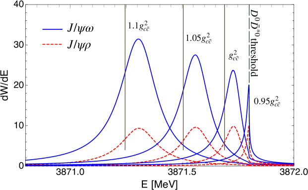
Figure 15: The transfer strength from the $c\bar{{c}}$ state to the final $J\!/\!\psi\omega$ and $J\!/\!\psi\rho$ states. Note that the energy abscissa is taken to be from 3870.8 to 3872 MeV. Final states are $J\!/\!\psi\omega$ (Solid lines), and $J\!/\!\psi\rho$ (dashed lines). The coupling $g_{c\bar{c}}^{2}$ is factored by 1.1, 1.05, 1, 0.95. The corresponding bound state energies calculated without the decay widths are shown by the left three vertical lines: 3871.25, 3871.51, and 3871.69 MeV, respectively. The most right vertical line corresponds to the $D^{0}\bar{{D}}{}^{*0}$ threshold. The one with the weakest coupling, 0.95$g_{c\bar{c}}^{2}$, does not have a bound state.

Namely, the peak energy of the final $J\!/\!\psi\pi^{n}$ is kept lower than or equal to the $D^{0}\bar{{D}}{}^{*0}$ threshold energy. On the other hand, the peak energy of the final $D^{0}\bar{{D}}{}^{*0}$ fraction is higher than threshold by definition. This means that the $X$(3872) mass is higher when measured by the final $D\bar{{D}}{}^{*}$ fraction, which is consistent with the observation. Experimentally the $X$(3872) mass observed by the $J/\psi$ and anything is 3871.69$\pm$0.17 MeV with a width of $<$1.2 MeV [5], while that of the final $D\bar{D}{}^{*}$ is 3872.9${+0.6\atop-0.4}{+0.4\atop-0.5}$ MeV [74] or 3875.1${+0.7\atop-0.5}\pm 0.5$ MeV[75]. The observed threshold mass is 3871.68$\pm$0.07 MeV [5]. Thus the mass observed by the $J/\psi$ and anything is consistent with the heavier two peaks in figure 15. This suggests that the $X$(3872) is either a virtual state or a very shallow bound state. These two states are very hard to distinguish from each other experimentally when one considers the width of the component, such as the $\rho$ meson. In literature, line shapes were studied by using amplitudes parametrized by effective range method [147] or by the Flatte parametrization [185, 186, 187]. It, however, seems difficult to determine the position of the resonance poles just from the shape of the decay spectrum. To discuss this subject, it will probably be necessary to treat the $\rho$ meson as a resonance of the $\pi\pi$ continuum and perform dynamical analyses.

In order to discuss possibilities of the other mechanism for the $X$(3872) peak as well as the effects of the meson decay width, let us ignore the OZI rule just for now. In strong decay, where the isospin is conserved, $J\!/\!\psi\rho$ does not directly decay from the $c\bar{c}$ core, but $J\!/\!\psi\omega$ may. We estimate the effects of existence of such a process by introducing a direct coupling between $J\!/\!\psi\omega$-$c\bar{c}$. Suppose the $J\!/\!\psi\omega$-$c\bar{c}$ coupling occurs by the same potential, $u$, there is a bound state with a binding energy of 10 MeV below the $D^{0}\bar{{D}}{}^{*0}$ threshold. But as seen in figure 16 and as expected, almost all the decay fraction is $J\!/\!\psi\omega$ and not $J\!/\!\psi\rho$ in that case, which is excluded by experiment. As far as $X$(3872) is concerned, no direct coupling seems to occur between the $c\bar{c}$ core and the $J/\psi\omega$ channel. One interesting point of this trial calculation is that the peak energy approaches the threshold as a less pronounced peak when the width of the $\omega$ meson is enlarged by hand. Therefore, exotic hadrons which appears at around a two-meson threshold and which contain meson(s) with a large decay width should be examined carefully. Let us make one more comment on the direct decay from the $c\bar{c}$ core. The $\chi_{c1}(2P)$ peak may not be seen in the $D\bar{{D}}{}^{*}$ decay spectrum, but it may be seen from the radiative decay. There is a selection rule of $E1$ transition that reduces the fraction $\chi_{c1}(2P)\to J/\psi\gamma$ but not $\to\psi(2S)\gamma$, which may show clearly the existence of $\chi_{c1}(2P)$ [188, 173], and if so, support the $c\bar{c}$ admixture of $X$(3872) discussed in this section.

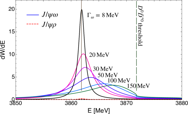
Figure 16: Trial calculation to estimate the effects of constructing mesons’ width. The $J\!/\!\psi\omega$ channel is assumed to couple to the $c\bar{c}$ core, and the width is enhanced by hand. (See text.) The solid line is for the final $J\!/\!\psi\omega$ fraction, the dashed line is for the final $J\!/\!\psi\rho$ fraction. The latter is shown only for $\Gamma_{\omega}$ = 8 MeV. The vertical lines correspond to the bound state energy and the ${D^{0}\bar{{D}}{}^{*0}}$ threshold.

Let us summarize the features of $X$(3872) and the $B$-decay to the final two-meson spectrum obtained in section 4. The two-meson and the $c\bar{c}$ hadron model which consists of the $c\bar{c}(1^{++})$ core, $D^{(*)0}\bar{{D}}{}^{(*)0}$ $({}^{3}S,{}^{3}D,{}^{5}D)$, $D^{(*)\pm}D^{(*)\mp}({}^{3}S,{}^{3}D,{}^{5}D)$, $J\!/\!\psi\omega$ and $J\!/\!\psi\rho^{0}$, the following features are obtained:

• $X$(3872) is a very shallow bound state or a virtual state which is close to the $D^{0}\bar{D}{}^{*0}$ threshold, which are very difficult to distinguish each other.

• The state is molecular, mostly $D^{0}\bar{D}{}^{*0}$ in the long range region, but has a considerable $D^{\pm}\bar{D}{}^{*\mp}$ component at the short distance.

• Two kinds of channel couplings provides attraction for $X$(3872): one is OPEP tensor, which mixes $D^{(*)}\bar{{D}}^{(*)}$ $S$-$D$-waves, the other is the $c\bar{c}$-$D\bar{D}{}^{*}$ coupling. These two effects are comparable in size.

• The amount of the $c\bar{c}$ component is found to be about 6 % in the model which contains both of the OPEP and the $c\bar{c}$-couplings, which meets the requirement from the production rate in the $p\bar{p}$ experiments.

• When considering the whole energy spectrum of the $B$ weak decay, there is one very narrow peak at the $D^{0}\bar{D}{}^{*0}$ threshold, but not around the $D^{\pm}\bar{D}{}^{*\mp}$ threshold, nor around the $c\bar{c}(1^{++})$ bare mass.

• Among the final products, amounts of $D\bar{{D}}^{*}$’s is the largest, which are produced directly from $c\bar{{c}}$ core. There are small amount of $J\!/\!\psi\omega$ and $J\!/\!\psi\rho$ final product, which are comparable to each other.

• The spectrum of the $J\!/\!\psi\omega$ and the $J\!/\!\psi\rho$ final products makes a very narrow peak at the bound state energy, if a bound state exists, or at the $D^{0}\bar{D}{}^{*0}$ threshold, if not. For instance, according to figure 15, the width is around 0.1 MeV when the binding energy is 0.5 MeV.

5 Charged heavy mesons

5.1 Brief overview in experimental status

Here we overview current experimental status about charged exotic mesons. We have summarized major experimental results of the charged charmonium-like and bottomonium-like exotic candidates in Table 11.

State	Mass [MeV]	Width [MeV]	Reaction	Exp. (Year)
$Z_{c}(3900)^{\pm}$	$3899.0\pm 3.6\pm 4.9$	$46\pm 10\pm 20$	$Y(4260)\to\pi^{+}\pi^{-}J/\psi$	BESIII(2013)
	$3894.5\pm 6.6\pm 4.5$	$63\pm 24\pm 26$	$Y(4260)\to\pi^{+}\pi^{-}J/\psi$	Belle(2013)
	$3886\pm 4\pm 2$	$37\pm 4\pm 8$	$\psi(4160)\to\pi^{+}\pi^{-}J/\psi$	CLEO-c(2013)
	$3883.9\pm 1.5\pm 4.2$	$24.8\pm 3.3\pm 11.0$	$Y(4260)\to(D\bar{D}^{\ast})^{\pm}\pi^{\mp}$	BESIII(2014)
	$3895.0\pm 5.2\pm^{+4.0}_{-2.7}$		$H_{b}\to J/\psi\pi^{+}\pi^{-}+X$	D0(2018)
$Z_{c}(3900)^{0}$	$3894.8\pm 2.3\pm 3.2$	$29.6\pm 8.2\pm 8.2$	$Y(4260)\to\pi^{0}\pi^{0}J/\psi$	BESIII(2015)
	$3885.7^{+4.3}_{-5.7}\pm 8.4$	$35^{+11}_{-12}\pm 15$	$Y(4260)\to(D\bar{D}^{\ast})^{0}\pi^{0}$	BESIII(2015)
$Z_{c}(4020)^{\pm}$	$4022.9\pm 0.8\pm 2.7$	$7.9\pm 2.7\pm 2.6$	$e^{+}e^{-}\to\pi^{+}\pi^{-}h_{c}$	BESIII(2013)
$Z_{c}(4025)^{\pm}$	$4026.3\pm 2.6\pm 3.7$	$24.8\pm 2.6\pm 7.7$	$Y(4260)\to(D^{\ast}\bar{D}^{\ast})^{\pm}\pi^{\mp}$	BESIII(2014)
$Z_{c}(4025)^{0}$	$4025.5^{+2.0}_{-4.7}\pm 3.1$	$23.0\pm 6.0\pm 1.0$	$Y(4260)\to(D^{\ast}\bar{D}^{\ast})^{0}\pi^{0}$	BESIII(2015)
$Z_{c}(4050)^{+}$	$4051\pm 14^{+20}_{-41}$	$82^{+21}_{-17}{}^{+47}_{-22}$	$\bar{B}^{0}\to\chi_{c1}(1P)K^{-}\pi^{+}$	Belle(2008)
$Z_{c}(4200)^{+}$	$4196^{+31}_{-29}{}^{+17}_{-13}$	$370^{+70}_{-70}{}^{+70}_{-132}$	$\bar{B}^{0}\to J/\psi K^{-}\pi^{+}$	Belle(2014)
$Z_{c}(4250)^{+}$	$4248^{+44}_{-29}{}^{+180}_{-35}$	$177^{+54}_{-39}{}^{+316}_{-61}$	$\bar{B}^{0}\to\chi_{c1}(1P)K^{-}\pi^{+}$	Belle(2008)
$Z_{c}(4430)^{+}$	$4433\pm 4\pm 2$	$45^{+18}_{-13}{}^{+30}_{-13}$	$B\to K\pi^{+}\psi(2S)$	Belle(2008)
$Z_{c}(4430)^{-}$	$4485^{+22+28}_{-22-11}$	$200^{+41+26}_{-46-35}$	$B^{0}\to K^{+}\pi^{-}\psi(2S)$	Belle(2013)
$Z_{c}(4430)^{-}$	$4475\pm 7^{+15}_{-25}$	$172\pm 13^{+37}_{-34}$	$B^{0}\to K^{+}\pi^{-}\psi(2S)$	LHCb(2014)
$Z_{b}(10610)^{\pm}$	$10607.2\pm 2.0$	$18.4\pm 2.4$	$\Upsilon(5S)\to\pi^{+}\pi^{-}\Upsilon(1,2,3S)$	Belle(2012)
			$\Upsilon(5S)\to\pi^{+}\pi^{-}h_{b}(1,2P)$
$Z_{b}(10610)^{0}$	$10609\pm 4\pm 4$	18.4 (input)	$\Upsilon(5S)\to\pi^{0}\pi^{0}\Upsilon(2,3S)$	Belle(2013)
$Z_{b}(10650)^{\pm}$	$10652.2\pm 1.5$	$11.5\pm 2.2$	$\Upsilon(5S)\to\pi^{+}\pi^{-}\Upsilon(1,2,3S)$	Belle(2012)
			$\Upsilon(5S)\to\pi^{+}\pi^{-}h_{b}(1,2P)$

Table 11: Experimental status of the charged charmonium-like and bottomonium-like exotic candidates with the neutral isospin partners.

Below, we pickup $Z_{c}(3900)$, $Z_{c}(4200)$, $Z_{c}(4430)$, $Z_{b}(10610)$ and $Z_{b}(10650)$, as well-known candidates. All these states have the quantum numbers $I^{G}(J^{PC})=1^{+}(1^{+-})$.

$Z_{c}(3900)$ with mass $3887.2\pm 2.3$ MeV and decay width $28.2\pm 2.6$ MeV was found in the decay of $Y(4260)$: $Y(4260)\rightarrow\pi^{\mp}Z_{c}(3900)^{\pm}$, $Z_{c}(3900)^{\pm}\rightarrow\pi^{\pm}J/\psi$ in BESIII [189] and was also confirmed by Belle [190] and CLEO [191]. The mass lies about 11 MeV above the $D^{+}\bar{D}^{\ast 0}$ (or 12 MeV above the $D^{\ast+}\bar{D}^{0}$) threshold. The process $e^{+}e^{-}\to\pi^{\pm}(D\bar{D}^{\ast})^{\mp}$ at $\sqrt{s}=4.26$ GeV was studied and the strong threshold enhancement, $Z_{c}(3885)$ with mass $3883.9\pm 1.5\pm 4.2$ MeV and width $24.8\pm 3.3\pm 11.0$ MeV was observed in [192]. In PDG [5], $Z_{c}(3885)$ is assumed to be related to $Z_{c}(3900)$. Its quantum numbers, $I^{G}(J^{P})=1^{+}(1^{+})$, have been determined in a partial wave analysis of the process $e^{+}e^{-}\to\pi^{+}\pi^{-}J/\psi$ by BESIII [193]. The decay $Z_{c}(3900)\rightarrow\pi^{\pm}h_{c}$ was not seen in BESIII [194].

The $\pm 1$ electric charge of the $Z_{c}(3900)^{\pm}$, indicating the quark contents $u\bar{d}c\bar{c}$ and $d\bar{u}c\bar{c}$, suggests the existence of the isospin partner, $(u\bar{u}-d\bar{d})c\bar{c}$. Indeed, a 3.5 $\sigma$ level significance evidence of a neutral $Z_{c}(3900)^{0}$ was reported in [191]. Later, $Z_{c}(3900)^{0}$ was also observed in $e^{+}e^{-}\rightarrow\pi^{0}Z_{c}(3900)^{0}\rightarrow\pi^{0}\pi^{0}J/\psi$ (10.4 $\sigma$) [195] and in $e^{+}e^{-}\rightarrow\pi^{0}Z_{c}(3900)^{0}\rightarrow\pi^{0}(D\bar{D}^{\ast})^{0}$ (greater than 10$\sigma$) [196].

Belle observed $Z_{c}(4200)$ via $Z_{c}(4200)\rightarrow J/\psi\pi^{+}$ in $\bar{B}^{0}\rightarrow K^{-}\pi^{+}J/\psi$, and it has mass $4196^{+31}_{-29}{}^{+17}_{-13}$ MeV and decay width $370^{+70}_{-70}{}^{+70}_{-132}$ MeV with the quantum numbers $I^{G}(J^{P})=1^{+}(1^{+-})$ [197]. LHCb found the evidence for $Z_{c}(4200)$ contributions to $\Lambda_{b}\to J/\psi p\pi^{-}$ decays [198], and found some structure where the invariant mass of $J/\psi\pi^{-}$ is near 4200 MeV in $B^{0}\to J/\psi K^{+}\pi^{-}$ decays [199].

$Z_{c}(4430)$ was first observed in Belle with the mass of $4433\pm 4\pm 2$ MeV [200]. The present world average of the mass, $4478^{+15}_{-18}$ MeV [5], is about 50 MeV higher than the original value, though the name $Z_{c}(4430)$ is still used. An interesting point is that $Z_{c}(4430)$ is first observed in the channel including the radially excited state of the charmonium $\psi(2S)$, not the ground state charmonium $J/\psi$. Dalitz analysis of $B\rightarrow K\pi\psi(2S)$ decays was performed in [201] and the full amplitude analysis of $B^{0}\rightarrow K^{+}\pi^{-}\psi(2S)$ decays was done in [202]. As for the quantum numbers of the $Z_{c}(4430)$, $J^{P}=1^{+}$ were favored in [202] and confirmed by LHCb [203]. LHCb also performed Argand diagram analysis and showed its resonance character.

The decay patterns of $Z_{c}(4430)$ exhibit interesting features:

$${\cal B}(B^{0}\rightarrow K^{+}Z_{c}^{-}(4430))\times{\cal B}(Z_{c}^{-}(4430)\rightarrow\pi^{-}\psi(2S))=(6.0^{+1.7+2.5}_{-2.0-1.4})\times 10^{-5}$$ (229)

from Ref. [202], and

$${\cal B}(\bar{B}^{0}\rightarrow K^{-}Z_{c}^{+}(4430))\times{\cal B}(Z_{c}^{+}(4430)\rightarrow\pi^{+}J/\psi)=(5.4^{+4.0+1.1}_{-1.0-0.9})\times 10^{-6}$$ (230)

from Ref. [197]. From the above two results, we obtain the branching ratio:

$$\frac{{\cal B}(Z_{c}^{-}(4430)\rightarrow\pi^{-}\psi(2S))}{{\cal B}(Z_{c}^{+}(4430)\rightarrow\pi^{+}J/\psi)}\simeq 10,$$ (231)

which indicates that the decay to $\pi\psi(2S)$ is enhanced relative to the decay to $\pi J/\psi$. This ordering is against the naive intuition; the decay rate to $\pi\psi(2S)$ should be smaller than the decay to $\pi J/\psi$ if only their phase space is considered. Further investigations will be useful for understanding the internal structure of the $Z_{c}(4430)$.

There are charged bottomonium-like states. The $Z_{b}^{\pm}(10610)$ and $Z_{b}^{\pm}(10650)$ were found in $\Upsilon(5S)\rightarrow\pi^{+}\pi^{-}\Upsilon(nS)$ ($n=1,2,3$) and $\Upsilon(5S)\rightarrow\pi^{+}\pi^{-}h_{b}(mP)$ ($m=1,2$) by Belle [204, 205]. $Z_{b}^{\pm}(10610)$ has the mass $10607.2\pm 2.0$ MeV and the decay width $18.4\pm 2.4$ MeV, and $Z_{b}^{\pm}(10650)$ has the mass $10652.2\pm 1.5$ MeV and the decay width $11.5\pm 2.2$ MeV. It is noted that their masses are very close to the $B\bar{B}^{\ast}$ and $B^{\ast}\bar{B}^{\ast}$ thresholds. The fact that $Z_{b}^{\pm}(10610)$ and $Z_{b}^{\pm}(10650)$ were found in $e^{+}e^{-}\rightarrow\Upsilon(nS)\pi^{+}\pi^{-}$ favors $I^{G}(J^{P})=1^{+}(1^{+})$, as it is expected from the final state when $S$-waves are assumed [205].

It is interesting that $Z_{b}^{\pm}(10610)$ and $Z_{b}^{\pm}(10650)$ have a larger probability in the decay to open heavy mesons rather than the decay to bottomonia; $Z_{b}^{\pm}(10610)\rightarrow B\bar{B}^{\ast}$ and $Z_{b}^{\pm}(10650)\rightarrow B^{\ast}\bar{B}^{\ast}$ are the dominant channels with the fractions about 86 % and 74 %, respectively [206]. For a charged state, $Z_{b}^{\pm}(10610)$ decays to $\pi\Upsilon(nS)$ ($n=1,2,3$) and to $\pi h_{b}(mP)$ ($n=1,2$) with the fractions whose values are of the same order. Situation is the same for the $Z_{b}^{\pm}(10650)$. This indicates that the heavy quark spin symmetry is violated largely for $Z_{b}^{\pm}(10610)$ and $Z_{b}^{\pm}(10650)$ [207]. $Z_{b}^{\pm}(10610)$ and $Z_{b}^{\pm}(10650)$ were also found in $\Upsilon(11020)\rightarrow h_{b}(nP)\pi^{+}\pi^{-}$ [208], where the mass of $\Upsilon(11020)$ lies above $\Upsilon(5S)$. The neutral partner, $Z_{b}^{0}(10610)$, was found in $\Upsilon(5S)\rightarrow\pi^{0}\pi^{0}\Upsilon(nS)$ ($n=1,2,3$) by Belle[209]. However, no significance signal was obtained for $Z_{b}^{0}(10650)$.

The structures of the charged charmonium-like and bottomoniumu-like states discussed above have been studied theoretically in the hadronic-molecular approaches [210, 211, 212, 213, 214, 59, 15, 215, 216, 217, 218, 219, 220, 221, 222, 223, 224, 225, 226, 227, 228, 229, 230, 231], in the hadrocharmonium approach [232], in the QCD sum rule approaches [233, 234, 235, 236, 237, 105, 238, 239, 240, 241, 242, 243, 244], in the tetraquark approaches [245, 246, 247, 248, 249, 250, 251, 252, 253, 254], in the heavy quark spin symmetry approaches [207, 100, 255, 256] and in the lattice QCD approaches [257, 258, 259, 260, 261, 262, 263]. The production and decay processes of the charged charmonium-like and bottomoniumu-like states have been studied in [264, 265, 266, 267, 268, 269, 270, 271, 272, 273, 274, 275, 276, 277, 278, 279, 280, 281, 282, 283, 284, 285, 286, 287, 288, 289, 290, 291, 292, 293, 294, 295, 296, 297, 298, 299, 300, 301, 302, 303, 304].

5.2 Isovector $P^{(\ast)}\bar{P}^{(\ast)}$ molecule with OPEP

In this subsection, we study how the $Z_{c}$ and $Z_{b}$ states are generated as isovector $P^{(\ast)}\bar{P}^{(\ast)}$ molecular state with the OPEP. We focus on the states with $J^{PC}=0^{++},$ $1^{+-}$ and $1^{++}$, where the $S$-wave $P^{(\ast)}\bar{P}^{(\ast)}$ component is included. Among them, $J^{PC}=1^{+-}$ is assigned as the quantum number of $Z_{c}(3900)$, $Z_{c}(4200)$, and $Z_{c}(4430)$. The $J^{PC}=1^{++}$ state has not been reported, but it is the isospin partner of $X(3872)$.

The components of the isovector $P^{(\ast)}\bar{P}^{(\ast)}$ states for $J^{PC}=0^{++},1^{++}$, and $1^{+-}$ are given by [12, 57]

$$0^{++}: P\bar{P}(^{1}S_{0}),P^{\ast}\bar{P}^{\ast}(^{1}S_{0},{{}^{5}D_{0}}),$$ (232)

$$1^{++}: \frac{1}{\sqrt{2}}\left(P\bar{P}^{\ast}-P^{\ast}\bar{P}\right)(^{3}S_{1},{{}^{3}D_{1}}),P^{\ast}\bar{P}^{\ast}(^{5}D_{1}),$$ (233)

$$1^{+-}: \frac{1}{\sqrt{2}}\left(P\bar{P}^{\ast}+P^{\ast}\bar{P}\right)(^{3}S_{1},{{}^{3}D_{1}}),P^{\ast}\bar{P}^{\ast}(^{3}S_{1},{{}^{3}D_{1}}).$$ (234)

The lowest threshold of the $J^{PC}=0^{++}$ state is $P\bar{P}$, while $P\bar{P}^{\ast}$ and $P^{\ast}\bar{P}$ are the lowest thresholds for $J^{PC}=1^{++}$ and $1^{+-}$. We note that the phase convention in (232)-(234) is different from the one in the literatures [12, 57] as discussed in section 3.7.

In the basis (232)-(234), the matrix elements of the OPEP in (92)-(95) are given by [12, 57]

$$V^{0^{++}}_{\pi}(r) = \left(\frac{g_{A}}{2f_{\pi}}\right)^{2}\frac{1}{3}\left(\begin{array}[]{ccc}0&-\sqrt{3}{\cal C}_{\pi}&\sqrt{6}{\cal T}_{\pi}\\ -\sqrt{3}{\cal C}_{\pi}&2C_{\pi}&\sqrt{2}T_{\pi}\\ \sqrt{6}{\cal T}_{\pi}&\sqrt{2}T_{\pi}&-C_{\pi}+2T_{\pi}\\ \end{array}\right),$$ (238)

$$V^{1^{++}}_{\pi}(r) = \left(\frac{g_{A}}{2f_{\pi}}\right)^{2}\frac{1}{3}\left(\begin{array}[]{ccc}-{\cal C}_{\pi}&\sqrt{2}{\cal T}_{\pi}&\sqrt{6}T_{\pi}\\ \sqrt{2}{\cal T}_{\pi}&-{\cal C}_{\pi}-{\cal T}_{\pi}&\sqrt{3}T_{\pi}\\ \sqrt{6}T_{\pi}&\sqrt{3}T_{\pi}&-C_{\pi}+T_{\pi}\\ \end{array}\right),$$ (242)

$$V^{1^{+-}}_{\pi}(r) = \left(\frac{g_{A}}{2f_{\pi}}\right)^{2}\frac{1}{3}\left(\begin{array}[]{cccc}{\cal C}_{\pi}&-\sqrt{2}{\cal T}_{\pi}&-2C_{\pi}&-\sqrt{2}T_{\pi}\\ -\sqrt{2}{\cal T}_{\pi}&{\cal C}_{\pi}+{\cal T}_{\pi}&-\sqrt{2}T_{\pi}&-2C_{\pi}+T_{\pi}\\ -2C_{\pi}&-\sqrt{2}T_{\pi}&C_{\pi}&-\sqrt{2}T_{\pi}\\ -\sqrt{2}T_{\pi}&-2C_{\pi}+T_{\pi}&-\sqrt{2}T_{\pi}&C_{\pi}+T_{\pi}\\ \end{array}\right),$$ (247)

where the functions ${\cal C}_{\pi}$, ${\cal T}_{\pi}$, $C_{\pi}$ and $T_{\pi}$ are given in (182). The potential form in the isovector channel is almost the same as the one in the isoscalar channel, while the isospin factors are different, ${\boldsymbol{\tau}}_{1}\cdot{\boldsymbol{\tau}}_{2}=+1$ for $I=1$ and ${\boldsymbol{\tau}}_{1}\cdot{\boldsymbol{\tau}}_{2}=-3$ for $I=0$, compare (247) and (182).

As in section 4.2, the $P^{(\ast)}\bar{P}^{(\ast)}$ state is studied by solving the coupled channel Schrödinger equation with the Hamiltonian

$$H^{J^{PC}} = K^{J^{PC}}+V^{J^{PC}}_{\pi}.$$ (248)

The kinetic term is given by

$$K^{0^{++}} = {\rm diag}\left(-\frac{1}{2\mu_{P\bar{P}}}\Delta_{0},-\frac{1}{2\mu_{P^{\ast}\bar{P}^{\ast}}}\Delta_{0}+2\Delta m_{PP^{\ast}},-\frac{1}{2\mu_{P^{\ast}\bar{P}^{\ast}}}\Delta_{2}+2\Delta m_{PP^{\ast}},\right)$$ (249)

$$K^{1^{++}} = {\rm diag}\left(-\frac{1}{2\mu_{P\bar{P}^{\ast}}}\Delta_{0},-\frac{1}{2\mu_{P\bar{P}^{\ast}}}\Delta_{2},-\frac{1}{2\mu_{P^{\ast}\bar{P}^{\ast}}}\Delta_{2}+\Delta m_{PP^{\ast}},\right)$$ (250)

$$K^{1^{+-}} = {\rm diag}\left(-\frac{1}{2\mu_{P\bar{P}^{\ast}}}\Delta_{0},-\frac{1}{2\mu_{P\bar{P}^{\ast}}}\Delta_{2},-\frac{1}{2\mu_{P^{\ast}\bar{P}^{\ast}}}\Delta_{0}+\Delta m_{PP^{\ast}},\right.$$ (251)

$$\left.-\frac{1}{2\mu_{P^{\ast}\bar{P}^{\ast}}}\Delta_{2}+\Delta m_{PP^{\ast}}\right),$$

where $\mu_{P^{(\ast)}\bar{P}^{(\ast)}}$, $\Delta_{\ell}$ and $\Delta m_{P^{(\ast)}\bar{P}^{(\ast)}}$ are defined in (185)-(187), and the masses of $P^{(\ast)}=D^{(\ast)},B^{(\ast)}$ are given in table 7.

As studied in section 4.2, we search the parameter region which gives a bound state by varying the parameters $g_{A}$ and $\Lambda$. As a result, the boundary of the isovector $D^{(\ast)}\bar{D}^{(\ast)}$ and $B^{(\ast)}\bar{B}^{(\ast)}$ bound states in the $(g_{A},\Lambda)$ plane is shown in figure 17. The results for $J^{PC}=0^{++}$ and $1^{+-}$ are similar, while we note that the lowest thresholds are different, $P\bar{P}$ for $J^{PC}=0^{++}$, and $P\bar{P}^{\ast}$ $(P^{\ast}\bar{P})$ for $J^{PC}=1^{+-}$. The bound region of the $J^{PC}=1^{++}$ is slightly larger than the others, and hence the attraction for $J^{PC}=1^{++}$ is larger than that for $J^{PC}=0^{++}$ and $1^{+-}$. Comparing the results of the $D^{(\ast)}\bar{D}^{(\ast)}$ and $B^{(\ast)}\bar{B}^{(\ast)}$ states, the $B^{(\ast)}\bar{B}^{(\ast)}$ bound region is wider than the $D^{(\ast)}\bar{D}^{(\ast)}$ one. This is because the heavier mass suppresses the kinetic energy, and because the the small $BB^{\ast}$ mass splitting enhances the attraction from the coupled channel effect. For the reference point $(g_{A},\Lambda)=(0.55,1.13\,{\rm GeV})$, no bound state is found for the isovector channels of both the charm and bottom sectors. To accommodate bound states, we need larger $g_{A}$ and/or $\Lambda$. In fact, our previous choice of the overestimated coupling strength corresponds to the vertical line $g_{A}\sim 0.83=\sqrt{2}\times 0.59$ [57] (see the footnote§ ‣ 3.4 in page § ‣ 3.4) which allowed a shallow bound state for the isovector $B^{(\ast)}\bar{B}^{(\ast)}$ channel. When we have only the OPEP, larger $g_{A}$ or $\Lambda$ is needed to produce a isovector $P^{(\ast)}\bar{P}^{\ast}$ bound state.

$J^{PC}=0^{++}$

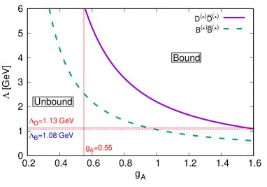
$J^{PC}=1^{++}$	$J^{PC}=1^{+-}$

Figure 17: The boundary lines of the isovector $P^{(\ast)}\bar{P}^{(\ast)}$ bound states in the $(g_{A},\Lambda)$ plane for $J^{PC}=0^{++}$, $1^{++}$ and $1^{+-}$. The results of the $D^{(\ast)}\bar{D}^{(\ast)}$ and $B^{(\ast)}\bar{B}^{(\ast)}$ states are shown by the solid and dashed lines, respectively. The right side beyond the line is the bound region, while the left side is the unbound region. The vertical solid lines is the values at $g_{A}=0.55$, while the horizontal solid and dashed lines are the values at $\Lambda=\Lambda_{D}=1.13$ GeV and $\Lambda=\Lambda_{B}=1.08$ GeV, respectively.

Finally, we compare the results for the isovector and isoscalar channels. In figure 18, the boundary lines of the $D^{(\ast)}\bar{D}^{(\ast)}$ bound states for $I(J^{PC})=I(1^{++})$ ($I=0,1$) are shown, which were obtained in figure 17 for $I=1$ and in figure 7 for $I=0$. As seen in figure 18, the bound region for $I=0$ is obviously larger than that for $I=1$. This fact indicates that the attraction in the $I=0$ channel is stronger than that in the $I=1$ channel. The difference between them comes from the isospin dependence of the OPEP, which is given by the isospin factor $\boldsymbol{\tau}_{1}\cdot\boldsymbol{\tau}_{2}$ in (92)-(95); ${\boldsymbol{\tau}}_{1}\cdot{\boldsymbol{\tau}}_{2}=-3$ for the isoscalar channel, while ${\boldsymbol{\tau}}_{1}\cdot{\boldsymbol{\tau}}_{2}=+1$ for the isovector channel. For the OPEP, the tensor force in the off-diagonal term has the dominant role to produce an attraction rather than the diagonal term. For the off-diagonal term, the sign of the potential is not important, but the magnitude is important because the off-diagonal term contributes as the second order of the perturbation. Thus, the attraction in the isoscalar channel with $|{\boldsymbol{\tau}}_{1}\cdot{\boldsymbol{\tau}}_{2}|=3$ is larger than that in the isovector one with $|{\boldsymbol{\tau}}_{1}\cdot{\boldsymbol{\tau}}_{2}|=1$ by about a factor $9$.

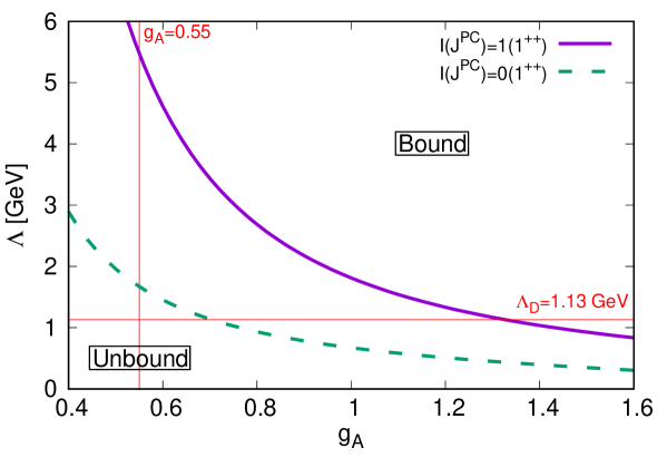
Figure 18: The boundary lines of the $D^{(\ast)}\bar{D}^{(\ast)}$ bound states $J^{PC}=1^{++}$ in the $(g_{A},\Lambda)$ plane for the isospin $I=1$ and $0$. The solid and dashed lines show the results for $I=1$ and for $I=0$, respectively, which are obtained in figure 17 and figure 7. The right side beyond the line is the bound region, while the left side is the unbound region. The vertical and horizontal solid lines show the values at $g_{A}=0.55$ and at $\Lambda=\Lambda_{D}=1.13$ GeV, respectively.

5.3 $P^{(\ast)}\bar{P}^{(\ast)}$ molecule with OPEP and $\sigma$ exchange potential

In the previous subsection, we have seen that the OPEP contribution is rather small in the isovector channel. In such a situation, the short and middle range interactions may become important. Such interaction includes $\sigma$, $\rho$ and $\omega$ exchange interactions [305]. In the isoscalar $P^{(\ast)}\bar{P}^{(\ast)}$ channel for $X(3872)$, we have not considered them because of a reason discussed below. In the isovector channel, there is another reason that we expect that the vector meson exchanges are not important; $\rho$ and $\omega$ exchange interactions have opposite signs and mostly cancel.

The $\sigma$ exchange potential may be effective not only for the isovector channel but also for the $X(3872)$ isoscalar channel. One of the reasons that we have considered only OPEP in the previous sections is that the effect of the short range interaction including the $\sigma$ exchange has been effectively taken care of by the suitable choice of the cutoff parameter $\Lambda$. To determine the reference value of $\Lambda$, we have used the binding energy of the deuteron. The OPEP thus determined for the nucleon-nucleon interaction is extrapolated to that of $D\bar{D}^{\ast}$ by assuming hadron structures by constituent quarks and the pion coupling to the light quarks. Strictly, however, we do not know to what extent such extrapolation works. Therefore, in this subsection we consider the role of $\sigma$-exchange interaction in some detail. Analysis here also provides an estimate of ambiguities coming from short range interactions.

The $\sigma$ exchange potential is derived by the effective Lagrangian of the heavy and $\sigma$ mesons [306],

$${\cal L}_{\sigma HH}=g_{\sigma}{\rm Tr}\left[H\sigma\bar{H}\right].$$ (252)

From this Lagrangian, the $\sigma$ exchange potential is obtained as

$$V^{\sigma}_{P\bar{P}{\mathchar 45\relax}P\bar{P}}(r)=-\left(\frac{g_{\sigma}}{m_{\sigma}}\right)^{2}C(r;m_{\sigma},\Lambda),$$ (253)

$$V^{\sigma}_{P\bar{P}^{\ast}{\mathchar 45\relax}P\bar{P}^{\ast}}(r)=-\left(\frac{g_{\sigma}}{m_{\sigma}}\right)^{2}C(r;m_{\sigma},\Lambda),$$ (254)

$$V^{\sigma}_{P^{\ast}\bar{P}^{\ast}{\mathchar 45\relax}P^{\ast}\bar{P}^{\ast}}(r)=-\left(\frac{g_{\sigma}}{m_{\sigma}}\right)^{2}C(r;m_{\sigma},\Lambda),$$ (255)

where the $\sigma$ mass $m_{\sigma}=550$ MeV is used. The factor $1/m^{2}_{\sigma}$ is multiplied because the function $C(r;m_{\sigma},\Lambda)$ includes $m^{2}_{\sigma}$ (see (87)).

There is ambiguity in the value of the coupling constant $g_{\sigma}$. In [305], $g_{\sigma}=3.65$ is taken, which is determined by a quark model estimation. This value is one-third of the value of the $\sigma NN$ coupling $g_{\sigma NN}$ according to the quark number counting, because the $\sigma$ meson couples to the scalar charge of hadrons which is additive. Another way to estimate $g_{\sigma}$ is to use a chiral theory for quarks such as the Nambu-Jona-Lasinio model [25, 26, 307]. By using the equality of the $\sigma qq$ and $\pi qq$ couplings, and the Goldberger-Treiman relation for the constituent quark, we have the relation

$$\frac{g_{\sigma}}{m_{q}}=\frac{g_{A}^{q}}{f_{\pi}}.$$ (256)

By using the parameter values $m_{q}\sim 300$ MeV, $f_{\pi}=93$ MeV, $g_{A}^{q}\sim 0.55$, we find $g_{\sigma}\sim 1.8$. Yet, in [306], an even smaller value $g_{\sigma}=g_{\pi}/2\sqrt{6}\sim 0.76$ is obtained, where $g_{\pi}=\Delta M/f_{\pi}$ and $\Delta M$ is the mass difference between the $0^{+}$ and $0^{-}$ heavy-light mesons. $\Delta M=349$ MeV is used in [306], which is the mass difference between $D^{\ast+}_{s0}$ and $D^{+}_{s}$. In this subsection, we present the results for $g_{\sigma}=0.76$ and $3.65$, which are regarded as the lower and upper limits of the attractive contribution due to the sigma meson exchange potential.

Using $\Lambda_{N}=681$ MeV for the $\pi\sigma$ potential for the nucleon as shown in table 4, $\Lambda_{D}$ and $\Lambda_{B}$ are obtained by $919$ MeV and $878$ MeV, respectively. In the basis of (232)-(233), the matrix elements of the $\sigma$ exchange potential for the given $J^{PC}$ are obtained by

$$V^{0^{++}}_{\sigma}(r) = -\left(\frac{g_{\sigma}}{m_{\sigma}}\right)^{2}\left(\begin{array}[]{ccc}C_{\sigma}&0&0\\ 0&C_{\sigma}&0\\ 0&0&C_{\sigma}\\ \end{array}\right),$$ (260)

$$V^{1^{++}}_{\sigma}(r) = -\left(\frac{g_{\sigma}}{m_{\sigma}}\right)^{2}\left(\begin{array}[]{ccc}C_{\sigma}&0&0\\ 0&C_{\sigma}&0\\ 0&0&C_{\sigma}\\ \end{array}\right),$$ (264)

$$V^{1^{+-}}_{\sigma}(r) = -\left(\frac{g_{\sigma}}{m_{\sigma}}\right)^{2}\left(\begin{array}[]{cccc}C_{\sigma}&0&0&0\\ 0&C_{\sigma}&0&0\\ 0&0&C_{\sigma}&0\\ 0&0&0&C_{\sigma}\\ \end{array}\right),$$ (269)

with the function $C_{\sigma}=C(r;m_{\sigma},\Lambda)$.

(i) $J^{PC}=0^{++}$

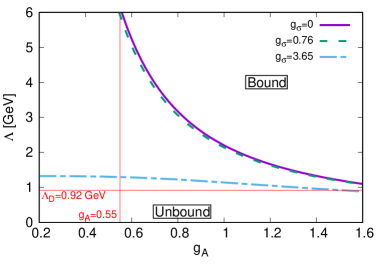
(ii) $J^{PC}=1^{++}$	(iii) $J^{PC}=1^{+-}$

Figure 19: The boundary of the isovector $D^{(\ast)}\bar{D}^{(\ast)}$ bound state with $V_{\pi}$ and $V_{\sigma}$ for (i) $J^{PC}=0^{++}$, (ii) $1^{++}$ and (iii) $1^{+-}$ in the $(g_{A},\Lambda)$ plane. The solid line shows the result for $g_{\sigma}=0$, namely only with $V_{\pi}$, while the dashed and dashed-dot lines are the results for $g_{\sigma}=0.76$ and $3.65$, respectively. The right side beyond the boundary line is the bound region, while the left side is the unbound region. The vertical and horizontal solid lines show the values at $g_{A}=0.55$ and at $\Lambda=\Lambda_{D}=0.92$ GeV, respectively.

In figure 19, the boundaries of the isovector $D^{(\ast)}\bar{D}^{(\ast)}$ bound states are shown for the case only with OPEP ($V_{\pi}$) is used and for the case of the $\pi\sigma$ exchange potential ($V_{\sigma}$) used in the $(g_{A},\Lambda)$ plane. The result with $g_{\sigma}=0$ is corresponds to the one only with the OPEP as shown in figure 17. Since $V_{\sigma}$ is attractive, the bound region for $g_{\sigma}\neq 0$ is larger than that for $g_{\sigma}=0$. For the small coupling $g_{\sigma}=0.76$, the boundary is close to the one for $g_{\sigma}=0$. Thus the $V_{\sigma}$ contribution is small, and the OPEP plays the dominant role. For $g_{\sigma}=3.65$, however, the bound region is much larger than that for $g_{\sigma}=0$ and $0.76$.

(i) $J^{PC}=0^{++}$

(ii) $J^{PC}=1^{++}$	(iii) $J^{PC}=1^{+-}$

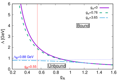
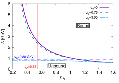
Figure 20: The boundary of the isovector $B^{(\ast)}\bar{B}^{(\ast)}$ bound state for (i) $J^{PC}=0^{++}$, (ii) $1^{++}$ and (iii) $1^{+-}$ in the $(g_{A},\Lambda)$ plane. The same convention is used as figure 19, while the vertical and horizontal solid lines show the values at $g_{A}=0.55$ and $\Lambda=\Lambda_{B}=0.88$ GeV, respectively.

The results for the isovector $B^{(\ast)}\bar{B}^{(\ast)}$ state are summarized in figure 20 for $J^{PC}=0^{++},1^{++}$ and $1^{+-}$. As seen in the $D^{(\ast)}\bar{D}^{(\ast)}$ state, the bound region of the $B^{(\ast)}\bar{B}^{(\ast)}$ state becomes large as the coupling $g_{\sigma}$ increases. The result for $g_{\sigma}=0.76$ is the similar to the one for $g_{\sigma}=0$. For $g_{\sigma}=3.65$, the bound region is much larger than those for $g_{\sigma}=0$ and $0.76$. For $(g_{A},\Lambda)=(0.55,0.88\,{\rm GeV})$, there are bound states for $J^{PC}=0^{++},1^{++}$ and $1^{+-}$. The binding energies are $0.92$ MeV for $0^{++}$, $1.51$ MeV for $1^{++}$, and $0.76$ MeV for $1^{+-}$. In experiments, however, the charged $Z^{(\prime)}_{b}$ states have been found above the $B^{(\ast)}\bar{B}^{(\ast)}$ threshold so far. The attraction generated by the interaction parameters $(g_{A},\Lambda)=(0.55,0.88\,{\rm GeV})$ could be overestimated. In the study of the hadronic molecules, the uncertainty of the parameters remains a problem, which should be addressed.

(i) $D^{(\ast)}\bar{D}^{(\ast)}$	(ii) $B^{(\ast)}\bar{B}^{(\ast)}$

Figure 21: The boundary of the isovector (i) $D^{(\ast)}\bar{D}^{(\ast)}$ and (ii) $B^{(\ast)}\bar{B}^{(\ast)}$ bound states in the $(g_{\sigma},\Lambda)$ plane. The vertical lines show the values at $g_{s}=0.76$ and $g_{s}=3.65$. The horizontal lines show the values at $\Lambda=\Lambda_{D}=0.92$ GeV for (i) $D^{(\ast)}\bar{D}^{(\ast)}$ and at $\Lambda=\Lambda_{B}=0.88$ GeV for (ii) $B^{(\ast)}\bar{B}^{(\ast)}$.

In the end, we show $g_{\sigma}$-$\Lambda$ plots to see continuously the change in the role of $\sigma$ exchange as $g_{\sigma}$ is varied figure 21. For the charm sector, the left figure indicates an unlikely situation for the molecular states to be generated at the mean value $g_{\sigma}\lesssim$ 1.8, where a very large cutoff is needed, $\Lambda\sim 4$ GeV. For bottom sector, the molecular states are not yet generated there, but only slight increase of $g_{\sigma}$ will do.

6 Pentaquark baryons

The discussion of exotic hadrons was activated when two new observations were reported in 2003; one is the $X(3872)$ which we have discussed in detail in this review, and the other the pentaquark $\Theta^{+}$ [308]. While the observation of the $X(3872)$ was rather accidental in the study of charmonium spectrum, that of $\Theta^{+}$ was motivated by the theoretical prediction by Diakonov et al [309]. The expected flavor quantum number $S=+1$ of the $\Theta^{+}$ requires the minimal quark content $uudd\bar{s}$, and hence the genuine multiquark exotic state. Various theoretical models have shown very different features, which was thought as an indication that we understood hadrons beyond the ground states only poorly. As in Ref. [309], a model of chiral symmetry with strong pionic soliton correlations predicts a positive parity state with a relatively low mass at around 1.5 GeV. The positive parity is also explained due to the strong pionic spin and isospin correlation [310]. One unique feature of this model is that the decay width is very narrow around 10 MeV or less. A model with strong diquark correlations can also make similar predictions, though their mechanisms are very much different [311]. Contrary, conventional quark model predicts a negative parity state at relatively large mass around 1.7 GeV or more and with a wide decay width [312]. Therefore, the experimental signals of mass at around 1.5 GeV with a narrow width seemed to support the chiral or diquark model.

After the first observation many data appeared supporting the $\Theta^{+}$, which are, however, followed by a number of experiments with no evidence [313]. There, more experimental data were taken and higher statistics analyses were done. In Ref. [314] how statistical fluctuations would have lead no evidence is discussed. One cannot, however, definitely conclude that these results have proven that the $\Theta^{+}$ does not exist. There are also discussions how multiquark exotics can be seen in some processes while not in the others [315]. It is particularly so when many experiments utilizes indirect processes induced by photons, leptons and hadrons (protons or pions) because the direct formation experiments, for instance, $K^{+}+n\to\Theta^{+}$ with a free neutron, is not possible. Therefore, we may expect further analyses with improved signal to noise ratio or direct experiments [316].

Aside from the $\Theta^{+}$, $\Lambda(1405)$ has long been an exotic baryon candidate that is described as a $\bar{K}N$ molecule [317, 318, 319, 5]. Its existence was first inferred by the analysis of $\bar{K}N$ scattering [11]. It is the lowest negative parity hyperon with an excitation energy of about 300 MeV. This amount is significantly small as compared to the others. For instance, the lowest negative parity nucleon $N(1535)$ is about 600 MeV above the ground state nucleon. This feature is not easy to be explained by the conventional quark model where baryons are made from three valence quarks. In Ref. [320], by introducing five quark states corresponding to the molecular channels such as $\bar{K}N$ coupled to the three-quark states, they have shown that the resonance structure at around 1405 MeV was generated.

Whether the picture of hadronic molecule $\bar{K}N$ crucially depends on the interaction between them. In the low energy theorem of chiral symmetry, the $\bar{K}N$ interaction appears attractive as given by the Weinberg-Tomozawa theorem. Physically, much of attraction strength is provided by $\omega$ meson exchange. At the quark level, it originates from the interaction between the antiquark $\bar{q}$ in the antikaon $\bar{K}$ and the quarks $q$ in the nucleon $N$. Due to charge conjugation, the sign of the vector type interaction flips from the one between quarks. Such a picture has been shown in the Skyrme model, which is one of successful chiral models for baryons [321, 322, 323, 324]. As a result, a $\bar{K}N$ bound state appears near the $\bar{K}N$ threshold. By coupling to the lower $\pi\Sigma$ channel, the bound state turns into a resonance, which is a typical mechanism of a Feshbach resonance. An experimental study of the $\bar{K}N$ molecule is going at J-PARC and analysis is underway [325, 326, 327].

Another important topic is the hidden charm $P_{c}$ baryons observed by LHCb in the weak decay $\Lambda_{b}\to J/\!\psi p\bar{K}$. Generally speaking, heavier constituents are more likely to be bound or resonate due to the suppression of their kinetic energies. Thus we expect more chances for exotic baryons. The first observation was reported in 2015 with a prominent peak structure in the invariant mass plot of $J/\!\psi p$ [328]. In their detailed analysis, they claimed that the peak was generated by two resonant states, one at 4380 MeV and the other at 4450 MeV. The analysis has been further performed with more statistics data in 2019, and they have reported three narrow peaks [19]; two at 4440 MeV and 4457 MeV that seem to split the strength of the former prominent peak, and one at 4312 MeV that was not seen in the former analysis. Thus they are denoted as $P_{c}(4312)^{+},P_{c}(4440)^{+}$ and $P_{c}(4457)^{+}$. Interestingly these three peaks are just below the thresholds; the higher two below $\Sigma_{c}\bar{D}^{*}$ threshold, and the lower one below the $\Sigma_{c}\bar{D}$ threshold.

The new observation has lead to a number of theory discussions of heavy quark multiplets formed by the four combinations of $\Sigma_{c},\Sigma_{c}^{*}$ and $\bar{D},\bar{D}^{*}$ [329, 330, 331, 332]. In the heavy quark limit, the pair of $\bar{D}$ and $\bar{D}^{*}$, and the pair of $\Sigma_{c}$ and $\Sigma_{c}^{*}$ are considered as a spin doublet of $J=0$ and 1, and the one of $J=1/2$ and 3/2, respectively. Their hadronic molecules also form multiplets of heavy quark spin symmetry. In connection with the present discussions, in the formation of these multiplets the tensor interaction of OPEP seem to play an important role [333]. It not only binds the constituent hadrons of these states but also splits the above two $P_{c}(4440)^{+}$, $P_{c}(4457)^{+}$ as a spin doublet.

Because the LHCb observed these states in the $J/\!\psi p$ final state, the isospin of these $P_{c}$ states is $I=1/2$. Therefore their masses are, respectively, 23 MeV and 6 MeV below the isospin averaged threshold of $\Sigma_{c}\bar{D}^{*}$, 4463 MeV. A relevant question is the origin of the masses, decay widths and quantum numbers of these states. Assuming that the orbital motion of the molecules is dominated by $S$-waves, possible total spin values are $J=1/2$ and 3/2. Now the crucial observation is that the tensor interaction can be effective for both states because the $S$-$D$ couplings survive for both channels. This is understood by the fact that the sum of $S(\Sigma_{c})=1/2,S(\bar{D}^{*})=1,L=0$ and the sum of $S(\Sigma_{c})=1/2,S(\bar{D}^{*})=1,L=2$ can both make the total spin $J=1/2$ and 3/2. This contrasts with the two nucleon system, where two states of $J=1$ and 0 are possible while the tensor force is effective only for the $J=1$ state (corresponding to the deuteron). Therefore, the two $P_{c}$’s provide an interesting opportunity to study the role of the tensor force in the OPEP.

Having said this much, in [333] the role of the tensor force in the OPEP has been discussed in a coupled channel model of $\Sigma_{c}^{(*)}\bar{D}^{(*)}$, $\Lambda_{c}\bar{D}^{(*)}$ with OPEP supplemented by the short range interaction that is brought about by the coupling of the molecular states with compact five quark states [334]. An interesting observation there is that by adjusting one most important model parameter for the short range interaction, they have made predictions of ten states. Three of them correspond to the $P_{c}$ states of the LHCb with good agreement with the observed masses and decay widths. The quantum numbers for the would be doublet $P_{c}(4440)$ and $P_{c}(4457)$ are then identified with $J=3/2$ and 1/2, respectively. It turns out that the mechanism of lowering the $J=3/2$ state is mostly due to the tensor force. The assignment of these quantum numbers is unique because the tensor force acts in the second order and the sign of the interaction does not matter. In general spin-spin interaction with heavy quark symmetry is employed to explain the splitting. However, the quantum numbers are not uniquely determined. Therefore, in Ref. [331], two options were investigated for the spin assignments. The spins of the $P_{c}$ states are not yet known, and hence the determination of them is very important for the further understanding of these states.

7 Summary and complements

7.1 Brief summary

In this article we have discussed the hadronic molecule as one of the exotic structures of hadrons. It has become possible experimentally to observe various exotic phenomena long after the predictions made more than half century ago, which have stimulated a diverse body of theoretical work. The ingredients of hadronic molecules are constituent hadrons and their interactions. The constituent hadrons also couple to compact structures. Therefore, we have discussed in detail how the admixture model has been applied to the $X(3872)$.

From a first-principle point of view, such a picture should effectively and conveniently replace the direct but complicated approach of QCD. In other words, the model should be economized [33, 335, 34], such that its work region, where and how, is under control. As emphasized in the introduction, hadronic molecules are expected to appear near threshold regions. Their formation is a consequence of finely tuned hadron dynamics, as their binding or resonant energies are of order MeV which is much smaller than the scale of low energy QCD, $\Lambda_{QCD}\sim$ some hundreds MeV. We have discussed why such conditions are likely to be realized for heavy hadrons. Their kinetic energies are suppressed and relatively weak force is sufficient to generate hadronic molecules.

For the interaction, we have emphasized the role of the one-pion exchange interaction. Pion dynamics are well established because the pion is the Nambu-Goldstone boson of spontaneous breaking of chiral symmetry, where the pion interaction is dictated by the low energy theorems. In the constituent quark picture the pion interacts with the light $u,d$ quarks by the pseudoscalar Yukawa coupling of $\boldsymbol{\sigma}\cdot\bi q$ type, whose strength is extracted from the empirically known axial coupling constants of hadrons.

The long range part of hadron interactions is provided by the OPEP, which we have discussed in detail in this paper. Because of the spin structure of the Yukawa coupling, the OPEP contributes to the transitions $D\to D^{*}$ and $D^{*}\to D^{*}$. It turns out that they are effective in the formation of a $D\bar{D}^{*}$ molecule for the $X(3872)$ channel . Therefore, an emphasis has been put on the role of the tensor component of the OPEP that causes mixing of states (channels) differing in angular momenta by 2$\hbar$. Because this transition leads to second order process, the resulting interaction for the relevant low lying channel must be attractive, with more attraction with more channel couplings.

There still remains a question for the short-range part, because the bare OPEP is singular. To avoid this we introduce a form factor. Such a prescription is known to work well for low energy properties of the deuteron [53] by employing a cutoff parameter around $\Lambda\sim 800$ MeV (see Table 4). To extend such a prescription to $DD^{*}$ molecule, in particular to determine the coupling strength and cutoff values for $DD^{*}$, we have employed a counting of quarks and the sizes of the nucleon and $D^{(*)}$ using the quark model.

It is interesting to note that the employed cutoff, $\Lambda\sim 800$ MeV for the nucleon, is consistent with the size of the nucleon core $\sqrt{6}/\Lambda\sim 0.5$ fm. Discussions of the nucleon core have a long history. It is recognized as the repulsive core of the $NN$ interaction, which has been explicitly shown in the study by the quark cluster model [336, 337]. It was also discussed in the chiral bag model where the nucleon is expressed as a quark core with pion clouds [338, 44].

Having this construction of the interactions, the OPEP provides a non-negligible amount of attraction particularly for hidden heavy hadrons such as $X(3872)$ with isospin 0, where the tensor force plays the dominant role, while the central component plays little. Therefore, the inclusion of the channel coupling of $SD$ waves (generally, states that differ in angular momenta by 2$\hbar$) is very important. The resulting strength of the attraction, however, turns out not to be sufficient to generate the $X(3872)$ as a molecular state of $D\bar{D}^{*}$. The coupling/mixing with a compact state of $c\bar{c}$ supplies additional attraction, if the compact state has a larger mass such as that theoretically expected for $\chi_{c1}(2P)$ charmonium meson. The mixing is also required to explain the large production rates of the $X(3872)$ in high energy hadron processes. Quantitative estimates of the production rate, however, have to be done carefully [133, 223, 144, 131, 132]. In the present analysis of the $X(3872)$, the OPEP and the short-range coupling play roughly equal roles. In general, however, their relative importance depends on the system under study.

Another possible molecule that we have discussed is the $Z_{c}(3900)$. However, the strength of the OPEP for the $Z_{c}(3900)$ of isospin one is smaller than that for the $X(3872)$ of isospin zero by factor three. As a result, the attraction is reduced and the formation of molecular state is less likely. In the remaining part of this article, we have also discussed the above features for the bottom sector.

7.2 Resonances or cusps

Here, we briefly mention a question which one would yet like to ask; whether the observed exotic phenomena imply physical resonant states or cusps of virtual states. At this moment, we have no decisive answer to this question for the observed signals, while there are many articles discussing the nature of the signals theoretically. Here we just refer only to a few of them in relation with the $X(3872)$ [185, 147, 186, 187, 339]. There, amplitude analyses are performed by using parametrizations of Flattè or effective range expansion types. Then an observation was made that by suitably choosing parameters, the line shape $X(3872)$ was shown to emerge as a virtual state cusp at the threshold [147].

To reproduce a very narrow or sharp peak at the $D^{0}\bar{D}^{*0}$ threshold, however, there must be sufficient amount of attraction between them. If the attraction is larger than the critical value, the peak appears as a resonant state, otherwise as a virtual state cusp. The difference between them is subtle because only a small change in the interaction strength may change the nature of the peak. Moreover, in such a situation it is difficult to differentiate them experimentally. But then the important question is; what would be the mechanism to provide that suitable amount of the attraction? In this paper, we have tried to offer an option that a model with the pion exchange interaction does it, supplemented by a coupling to a short distance structure. This is a dynamical approach for the construction of amplitudes that we discuss shortly below.

7.3 Hadron interactions and exotics

The last issue that we would like to mention is the dynamical approach for the construction of amplitudes from reliable hadron interactions. For heavy hadrons including charm or bottom quarks, it is formidably difficult to derive interactions from experiments. This is the reason that we have resorted to a model for the study of the the $X(3872)$ in this paper.

Yet another powerful and promising method is lattice QCD, which is, in principle, the first principle method for the strong interaction. In the so called HAL QCD method, hadron interactions are obtained by using the Nambu-Bethe-Salpeter amplitude [340, 341]. To obtain hadron interactions, this method is practically more powerful than the widely used Luscher’s method [342, 343]. An attempt was made for the $Z_{c}(3900)$ with coupled channels of $D\bar{D}^{*}$, $\eta_{c}\rho$, $J/\!\psi\pi$, where they have derived the interactions between these channels and solved the coupled channel problem [262, 263]. Unexpectedly it was found that there is a rather strong coupling between $J/\!\psi\pi$ and $D\bar{D}^{*}$ channels, which effectively causes an attraction in the $J/\!\psi\pi$ channel. As a consequence, they have found rather than a resonance, a virtual state pole that contributes to an enhancement near the $D\bar{D}^{*}$ threshold corresponding to $Z_{c}(3900)$.

For the study of exotic hadrons, an approach based on the coupled channel method with suitable hadron interactions is highly desired. It is a non-trivial program because many channels may couple, including those with more than two particles. With complementary approaches of experiments, effective theories and lattice simulations, such an approach can be further elaborated, thereby enabling elucidation of the nature of exotic hadrons.

References

References

- [1] Choi S K et al. (Belle) 2003 Phys. Rev. Lett. 91 262001 (Preprint hep-ex/0309032)
- [2] Aubert B et al. (BaBar) 2005 Phys. Rev. D71 031501 (Preprint hep-ex/0412051)
- [3] Gell-Mann M 1964 Phys.Lett. 8 214–215
- [4] Aaij R et al. (LHCb) 2013 Phys. Rev. Lett. 110 222001 (Preprint 1302.6269)
- [5] Tanabashi M et al. (Particle Data Group) 2018 Phys. Rev. D98 030001
- [6] Brambilla N et al. 2011 Eur. Phys. J. C71 1534 (Preprint 1010.5827)
- [7] Jaffe R L 1977 Phys.Rev. D15 267
- [8] Jaffe R L 1977 Phys.Rev. D15 281
- [9] Maiani L, Piccinini F, Polosa A D and Riquer V 2005 Phys. Rev. D71 014028 (Preprint hep-ph/0412098)
- [10] Terasaki K 2007 Prog. Theor. Phys. 118 821–826 (Preprint 0706.3944)
- [11] Dalitz R and Tuan S 1959 Phys.Rev.Lett. 2 425–428
- [12] Tornqvist N A 1994 Z. Phys. C61 525–537 (Preprint hep-ph/9310247)
- [13] Close F E and Page P R 2005 Phys.Lett. B628 215–222 (Preprint hep-ph/0507199)
- [14] Kou E and Pene O 2005 Phys.Lett. B631 164–169 (Preprint hep-ph/0507119)
- [15] Voloshin M B 2013 Phys. Rev. D87 091501 (Preprint 1304.0380)
- [16] Karliner M, Rosner J L and Skwarnicki T 2018 Ann. Rev. Nucl. Part. Sci. 68 17–44 (Preprint 1711.10626)
- [17] Karliner M 2019 JPS Conf. Proc. 26 011005
- [18] De Rujula A, Georgi H and Glashow S 1977 Phys.Rev.Lett. 38 317
- [19] Aaij R et al. (LHCb) 2019 Phys. Rev. Lett. 122 222001 (Preprint 1904.03947)
- [20] Hoyle F 1954 Astrophys.J.Suppl. 1 121–146
- [21] Ikeda K, Takigawa N and Horiuchi H 1968 Progress of Theoretical Physics Suppl. E68 464–475
- [22] Braaten E and Hammer H W 2007 Annals Phys. 322 120–163 (Preprint cond-mat/0612123)
- [23] Naidon P and Endo S 2017 Rept. Prog. Phys. 80 056001 (Preprint 1610.09805)
- [24] Guo F K, Hanhart C, Meißner U G, Wang Q, Zhao Q and Zou B S 2018 Rev. Mod. Phys. 90 015004 (Preprint 1705.00141)
- [25] Nambu Y and Jona-Lasinio G 1961 Phys. Rev. 122 345–358
- [26] Nambu Y and Jona-Lasinio G 1961 Phys. Rev. 124 246–254
- [27] Nagata S, Sasakawa T, Sawada T and Tamagaki R 1959 Progress of Theoretical Physics 22 274–298
- [28] Terasawa T 1960 Progress of Theoretical Physics 23 87–105
- [29] Pieper S C and Wiringa R B 2001 Ann. Rev. Nucl. Part. Sci. 51 53–90 (Preprint nucl-th/0103005)
- [30] Carlson J, Gandolfi S, Pederiva F, Pieper S C, Schiavilla R, Schmidt K E and Wiringa R B 2015 Rev. Mod. Phys. 87 1067 (Preprint 1412.3081)
- [31] Otsuka T, Suzuki T, Fujimoto R, Grawe H and Akaishi Y 2005 Phys. Rev. Lett. 95 232502
- [32] Myo T, Kato K, Toki H and Ikeda K 2007 Phys. Rev. C76 024305 (Preprint 0706.2911)
- [33] Weinberg S 1963 Phys. Rev. 130 776–783
- [34] Weinberg S 1965 Phys. Rev. 137 B672–B678
- [35] Nagahiro H and Hosaka A 2013 Phys. Rev. C88 055203 (Preprint 1307.2031)
- [36] Nagahiro H and Hosaka A 2014 Phys. Rev. C90 065201 (Preprint 1406.3684)
- [37] Sekihara T, Hyodo T and Jido D 2015 PTEP 2015 063D04 (Preprint 1411.2308)
- [38] Takeuchi S, Shimizu K and Takizawa M 2014 PTEP 2014 123D01 [Erratum: PTEP2015,no.7,079203(2015)] (Preprint 1408.0973)
- [39] Casalbuoni R, Deandrea A, Di Bartolomeo N, Gatto R, Feruglio F and Nardulli G 1997 Phys. Rept. 281 145–238 (Preprint hep-ph/9605342)
- [40] Manohar A V and Wise M B 2000 Heavy quark physics (Cambridge, England: Cambridge University Press)
- [41] Weinberg S 1968 Phys. Rev. 166 1568–1577
- [42] Coleman S R, Wess J and Zumino B 1969 Phys. Rev. 177 2239–2247
- [43] Callan Jr C G, Coleman S R, Wess J and Zumino B 1969 Phys. Rev. 177 2247–2250
- [44] Hosaka A and Toki H 2001 Quarks, baryons and chiral symmetry (Singapore, Singapore: World Scientific)
- [45] Bando M, Kugo T, Uehara S, Yamawaki K and Yanagida T 1985 Phys. Rev. Lett. 54 1215
- [46] Bando M, Kugo T and Yamawaki K 1988 Phys. Rept. 164 217–314
- [47] Nagahiro H, Yasui S, Hosaka A, Oka M and Noumi H 2017 Phys. Rev. D95 014023 (Preprint 1609.01085)
- [48] Cohen T D and Hansen J M 1998 Phys. Lett. B440 233–238 (Preprint nucl-th/9808006)
- [49] Epelbaum E and Gegelia J 2009 Eur. Phys. J. A41 341–354 (Preprint 0906.3822)
- [50] Nagels M M, Rijken T A and de Swart J J 1977 Phys. Rev. D15 2547
- [51] Rijken T A, Stoks V G J and Yamamoto Y 1999 Phys. Rev. C59 21–40 (Preprint nucl-th/9807082)
- [52] Machleidt R, Holinde K and Elster C 1987 Phys. Rept. 149 1–89
- [53] Ericson T E O and Weise W 1988 Pions and Nuclei vol 74 (Oxford, UK: Clarendon Press) ISBN 0198520085 URL http://www-spires.fnal.gov/spires/find/books/www?cl=QC793.5.M42E75::1988
- [54] Yamaguchi Y, Ohkoda S, Yasui S and Hosaka A 2011 Phys. Rev. D84 014032 (Preprint 1105.0734)
- [55] Yasui S and Sudoh K 2009 Phys. Rev. D80 034008 (Preprint 0906.1452)
- [56] Yamaguchi Y, Ohkoda S, Yasui S and Hosaka A 2012 Phys. Rev. D85 054003 (Preprint 1111.2691)
- [57] Ohkoda S, Yamaguchi Y, Yasui S, Sudoh K and Hosaka A 2012 Phys. Rev. D86 014004 (Preprint 1111.2921)
- [58] Ohkoda S, Yamaguchi Y, Yasui S, Sudoh K and Hosaka A 2012 Phys. Rev. D86 034019 (Preprint 1202.0760)
- [59] Yamaguchi Y, Ohkoda S, Yasui S and Hosaka A 2013 Phys. Rev. D87 074019 (Preprint 1301.4557)
- [60] Yamaguchi Y, Yasui S and Hosaka A 2014 Nucl. Phys. A927 110–118 (Preprint 1309.4324)
- [61] Geng L S, Lu J X, Valderrama M P and Ren X L 2018 Phys. Rev. D97 091501 (Preprint 1705.00516)
- [62] Peskin M E and Schroeder D V 1995 An Introduction to quantum field theory (Reading, USA: Addison-Wesley) ISBN 9780201503975, 0201503972 URL http://www.slac.stanford.edu/~mpeskin/QFT.html
- [63] Swanson E S 2004 Phys. Lett. B588 189–195 (Preprint hep-ph/0311229)
- [64] Thomas C E and Close F E 2008 Phys. Rev. D78 034007 (Preprint 0805.3653)
- [65] Acosta D et al. (CDF) 2004 Phys. Rev. Lett. 93 072001 (Preprint hep-ex/0312021)
- [66] Abazov V M et al. (D0) 2004 Phys. Rev. Lett. 93 162002 (Preprint hep-ex/0405004)
- [67] Aubert B et al. (BaBar) 2005 Phys. Rev. D71 071103 (Preprint hep-ex/0406022)
- [68] Aaij R et al. (LHCb) 2012 Eur. Phys. J. C72 1972 (Preprint 1112.5310)
- [69] Chatrchyan S et al. (CMS) 2013 JHEP 04 154 (Preprint 1302.3968)
- [70] Aaboud M et al. (ATLAS) 2017 JHEP 01 117 (Preprint 1610.09303)
- [71] Ablikim M et al. (BESIII) 2014 Phys. Rev. Lett. 112 092001 (Preprint 1310.4101)
- [72] Choi S K et al. 2011 Phys. Rev. D84 052004 (Preprint 1107.0163)
- [73] Aaltonen T et al. (CDF) 2009 Phys. Rev. Lett. 103 152001 (Preprint 0906.5218)
- [74] Aushev T et al. (Belle) 2010 Phys. Rev. D81 031103 (Preprint 0810.0358)
- [75] Aubert B et al. (BaBar) 2008 Phys. Rev. D77 011102 (Preprint 0708.1565)
- [76] Gokhroo G et al. (Belle) 2006 Phys. Rev. Lett. 97 162002 (Preprint hep-ex/0606055)
- [77] Abulencia A et al. (CDF) 2007 Phys. Rev. Lett. 98 132002 (Preprint hep-ex/0612053)
- [78] Aubert B et al. (BaBar) 2006 Phys. Rev. D74 071101 (Preprint hep-ex/0607050)
- [79] Aubert B et al. (BaBar) 2009 Phys. Rev. Lett. 102 132001 (Preprint 0809.0042)
- [80] Bhardwaj V et al. (Belle) 2011 Phys. Rev. Lett. 107 091803 (Preprint 1105.0177)
- [81] Aaij R et al. (LHCb) 2014 Nucl. Phys. B886 665–680 (Preprint 1404.0275)
- [82] Aaij R et al. (LHCb) 2015 Phys. Rev. D92 011102 (Preprint 1504.06339)
- [83] Aubert B et al. (BaBar) 2008 Phys. Rev. D77 111101 (Preprint 0803.2838)
- [84] Ablikim M et al. (BESIII) 2019 Phys. Rev. Lett. 122 232002 (Preprint 1903.04695)
- [85] Barnes T and Godfrey S 2004 Phys. Rev. D69 054008 (Preprint hep-ph/0311162)
- [86] Donoghue J F, Golowich E and Holstein B R 1992 Camb. Monogr. Part. Phys. Nucl. Phys. Cosmol. 2 1–540 [Camb. Monogr. Part. Phys. Nucl. Phys. Cosmol.35(2014)]
- [87] Bali G S 2001 Phys. Rept. 343 1–136 (Preprint hep-ph/0001312)
- [88] Barnes T, Godfrey S and Swanson E S 2005 Phys. Rev. D72 054026 (Preprint hep-ph/0505002)
- [89] Ebert D, Faustov R N and Galkin V O 2006 Phys. Lett. B634 214–219 (Preprint hep-ph/0512230)
- [90] Dubnicka S, Dubnickova A Z, Ivanov M A and Korner J G 2010 Phys. Rev. D81 114007 (Preprint 1004.1291)
- [91] Kim H, Kim K S, Cheoun M K, Jido D and Oka M 2016 Eur. Phys. J. A52 184 (Preprint 1602.07540)
- [92] Close F E and Page P R 2004 Phys. Lett. B578 119–123 (Preprint hep-ph/0309253)
- [93] Voloshin M B 2004 Phys. Lett. B579 316–320 (Preprint hep-ph/0309307)
- [94] Tornqvist N A 2004 Phys. Lett. B590 209–215 (Preprint hep-ph/0402237)
- [95] AlFiky M T, Gabbiani F and Petrov A A 2006 Phys. Lett. B640 238–245 (Preprint hep-ph/0506141)
- [96] Ding G J, Liu J F and Yan M L 2009 Phys. Rev. D79 054005 (Preprint 0901.0426)
- [97] Lee I W, Faessler A, Gutsche T and Lyubovitskij V E 2009 Phys. Rev. D80 094005 (Preprint 0910.1009)
- [98] Gamermann D, Nieves J, Oset E and Ruiz Arriola E 2010 Phys. Rev. D81 014029 (Preprint 0911.4407)
- [99] Li N and Zhu S L 2012 Phys. Rev. D86 074022 (Preprint 1207.3954)
- [100] Guo F K, Hidalgo-Duque C, Nieves J and Valderrama M P 2013 Phys. Rev. D88 054007 (Preprint 1303.6608)
- [101] Wang P and Wang X G 2013 Phys. Rev. Lett. 111 042002 (Preprint 1304.0846)
- [102] Baru V, Epelbaum E, Filin A A, Hanhart C, Meissner U G and Nefediev A V 2013 Phys. Lett. B726 537–543 (Preprint 1306.4108)
- [103] Garzon E J, Molina R, Hosaka A and Oset E 2014 Phys. Rev. D89 014504 (Preprint 1310.0972)
- [104] Jansen M, Hammer H W and Jia Y 2014 Phys. Rev. D89 014033 (Preprint 1310.6937)
- [105] Wang Z G and Huang T 2014 Eur. Phys. J. C74 2891 (Preprint 1312.7489)
- [106] Tomaradze A, Dobbs S, Xiao T and Seth K K 2015 Phys. Rev. D91 011102 (Preprint 1501.01658)
- [107] Baru V, Epelbaum E, Filin A A, Guo F K, Hammer H W, Hanhart C, Meißner U G and Nefediev A V 2015 Phys. Rev. D91 034002 (Preprint 1501.02924)
- [108] Braaten E 2015 Phys. Rev. D91 114007 (Preprint 1503.04791)
- [109] Wang Z Y, Qi J J, Guo X H and Wang C 2018 Phys. Rev. D97 016015 (Preprint 1710.07424)
- [110] Schmidt M, Jansen M and Hammer H W 2018 Phys. Rev. D98 014032 (Preprint 1804.00375)
- [111] Matheus R D, Navarra F S, Nielsen M and Zanetti C M 2009 Phys. Rev. D80 056002 (Preprint 0907.2683)
- [112] Danilkin I V and Simonov Yu A 2010 Phys. Rev. Lett. 105 102002 (Preprint 1006.0211)
- [113] Coito S, Rupp G and van Beveren E 2011 Eur. Phys. J. C71 1762 (Preprint 1008.5100)
- [114] Coito S, Rupp G and van Beveren E 2013 Eur. Phys. J. C73 2351 (Preprint 1212.0648)
- [115] Takizawa M and Takeuchi S 2013 PTEP 2013 093D01 (Preprint 1206.4877)
- [116] Ferretti J, Galatà G and Santopinto E 2013 Phys. Rev. C88 015207 (Preprint 1302.6857)
- [117] Chen W, Jin H y, Kleiv R T, Steele T G, Wang M and Xu Q 2013 Phys. Rev. D88 045027 (Preprint 1305.0244)
- [118] Ferretti J, Galatà G and Santopinto E 2014 Phys. Rev. D90 054010 (Preprint 1401.4431)
- [119] Zhou Z Y and Xiao Z 2017 Phys. Rev. D96 054031 [Erratum: Phys. Rev.D96,no.9,099905(2017)] (Preprint 1704.04438)
- [120] Yang Y B, Chen Y, Gui L C, Liu C, Liu Y B, Liu Z, Ma J P and Zhang J B (CLQCD) 2013 Phys. Rev. D87 014501 (Preprint 1206.2086)
- [121] Prelovsek S and Leskovec L 2013 Phys. Rev. Lett. 111 192001 (Preprint 1307.5172)
- [122] Lee S H, Detar C, Mohler D and Na H (Fermilab Lattice, MILC) 2014 PoS LATTICE2014 125
- [123] Padmanath M, Lang C B and Prelovsek S 2015 Phys. Rev. D92 034501 (Preprint 1503.03257)
- [124] Abe K et al. (Belle) 2005 Evidence for X(3872) gamma J/psi and the sub-threshold decay X(3872) omega J/psi Lepton and photon interactions at high energies. Proceedings, 22nd International Symposium, LP 2005, Uppsala, Sweden, June 30-July 5, 2005 (Preprint hep-ex/0505037)
- [125] del Amo Sanchez P et al. (BaBar) 2010 Phys. Rev. D82 011101 (Preprint 1005.5190)
- [126] Braaten E and Kusunoki M 2005 Phys. Rev. D72 054022 (Preprint hep-ph/0507163)
- [127] Suzuki M 2005 Phys. Rev. D72 114013 (Preprint hep-ph/0508258)
- [128] Terasaki K 2010 Prog. Theor. Phys. 122 1285–1290 (Preprint 0904.3368)
- [129] Zhou Z Y and Xiao Z 2018 Phys. Rev. D97 034011 (Preprint 1711.01930)
- [130] Ablikim M et al. (BESIII) 2019 Phys. Rev. Lett. 122 202001 (Preprint 1901.03992)
- [131] Braaten E, Kusunoki M and Nussinov S 2004 Phys. Rev. Lett. 93 162001 (Preprint hep-ph/0404161)
- [132] Braaten E and Kusunoki M 2005 Phys. Rev. D71 074005 (Preprint hep-ph/0412268)
- [133] Bignamini C, Grinstein B, Piccinini F, Polosa A D and Sabelli C 2009 Phys. Rev. Lett. 103 162001 (Preprint 0906.0882)
- [134] Zanetti C M, Nielsen M and Matheus R D 2011 Phys. Lett. B702 359–363 (Preprint 1105.1343)
- [135] Cho S and Lee S H 2013 Phys. Rev. C88 054901 (Preprint 1302.6381)
- [136] Denig A, Guo F K, Hanhart C and Nefediev A V 2014 Phys. Lett. B736 221–225 (Preprint 1405.3404)
- [137] Martinez Torres A, Khemchandani K P, Navarra F S, Nielsen M and Abreu L M 2014 Phys. Rev. D90 114023 [Erratum: Phys. Rev.D93,no.5,059902(2016)] (Preprint 1405.7583)
- [138] Larionov A B, Strikman M and Bleicher M 2015 Phys. Lett. B749 35–43 (Preprint 1502.03311)
- [139] Wang W and Zhao Q 2016 Phys. Lett. B755 261–264 (Preprint 1512.03123)
- [140] Abreu L M 2016 PTEP 2016 103B01 (Preprint 1608.08165)
- [141] Meng C, Han H and Chao K T 2017 Phys. Rev. D96 074014 (Preprint 1304.6710)
- [142] Albaladejo M, Guo F K, Hanhart C, Meißner U G, Nieves J, Nogga A and Yang Z 2017 Chin. Phys. C41 121001 (Preprint 1709.09101)
- [143] Esposito A, Grinstein B, Maiani L, Piccinini F, Pilloni A, Polosa A D and Riquer V 2018 Chin. Phys. C42 114107 (Preprint 1709.09631)
- [144] Esposito A, Pilloni A and Polosa A D 2017 Phys. Rept. 668 1–97 (Preprint 1611.07920)
- [145] Swanson E S 2004 Phys. Lett. B598 197–202 (Preprint hep-ph/0406080)
- [146] Navarra F S and Nielsen M 2006 Phys. Lett. B639 272–277 (Preprint hep-ph/0605038)
- [147] Braaten E and Lu M 2007 Phys. Rev. D76 094028 (Preprint 0709.2697)
- [148] Dubynskiy S and Voloshin M B 2008 Phys. Rev. D77 014013 (Preprint 0709.4474)
- [149] Braaten E and Lu M 2008 Phys. Rev. D77 014029 (Preprint 0710.5482)
- [150] Fleming S and Mehen T 2008 Phys. Rev. D78 094019 (Preprint 0807.2674)
- [151] Artoisenet P, Braaten E and Kang D 2010 Phys. Rev. D82 014013 (Preprint 1005.2167)
- [152] Fleming S and Mehen T 2012 Phys. Rev. D85 014016 (Preprint 1110.0265)
- [153] Braaten E and Kang D 2013 Phys. Rev. D88 014028 (Preprint 1305.5564)
- [154] Guo F K, Hidalgo-Duque C, Nieves J, Ozpineci A and Valderrama M P 2014 Eur. Phys. J. C74 2885 (Preprint 1404.1776)
- [155] Meng C, Sanz-Cillero J J, Shi M, Yao D L and Zheng H Q 2015 Phys. Rev. D92 034020 (Preprint 1411.3106)
- [156] Mehen T 2015 Phys. Rev. D92 034019 (Preprint 1503.02719)
- [157] Kang X W and Oller J A 2017 Eur. Phys. J. C77 399 (Preprint 1612.08420)
- [158] Ferretti J and Santopinto E 2019 Phys. Lett. B789 550–555 (Preprint 1806.02489)
- [159] Colangelo P, De Fazio F and Nicotri S 2007 Phys. Lett. B650 166–171 (Preprint hep-ph/0701052)
- [160] Dong Y b, Faessler A, Gutsche T and Lyubovitskij V E 2008 Phys. Rev. D77 094013 (Preprint 0802.3610)
- [161] Nielsen M and Zanetti C M 2010 Phys. Rev. D82 116002 (Preprint 1006.0467)
- [162] Wang T H and Wang G L 2011 Phys. Lett. B697 233–237 (Preprint 1006.3363)
- [163] Harada M and Ma Y L 2011 Prog. Theor. Phys. 126 91–113 (Preprint 1010.3607)
- [164] Mehen T and Springer R 2011 Phys. Rev. D83 094009 (Preprint 1101.5175)
- [165] Dubnicka S, Dubnickova A Z, Ivanov M A, Koerner J G, Santorelli P and Saidullaeva G G 2011 Phys. Rev. D84 014006 (Preprint 1104.3974)
- [166] Ke H W and Li X Q 2011 Phys. Rev. D84 114026 (Preprint 1107.0443)
- [167] Badalian A M, Orlovsky V D, Simonov Yu A and Bakker B L G 2012 Phys. Rev. D85 114002 (Preprint 1202.4882)
- [168] Margaryan A and Springer R P 2013 Phys. Rev. D88 014017 (Preprint 1304.8101)
- [169] Guo F K, Hanhart C, Meissner U G, Wang Q and Zhao Q 2013 Phys. Lett. B725 127–133 (Preprint 1306.3096)
- [170] Guo F K, Hanhart C, Kalashnikova Yu S, Meißner U G and Nefediev A V 2015 Phys. Lett. B742 394–398 (Preprint 1410.6712)
- [171] Cardoso M, Rupp G and van Beveren E 2015 Eur. Phys. J. C75 26 (Preprint 1411.1654)
- [172] Badalian A M, Simonov Yu A and Bakker B L G 2015 Phys. Rev. D91 056001 (Preprint 1501.01168)
- [173] Takeuchi S, Takizawa M and Shimizu K 2017 JPS Conf. Proc. 17 112001 (Preprint 1602.04297)
- [174] Swanson E S 2006 Phys. Rept. 429 243–305 (Preprint hep-ph/0601110)
- [175] Godfrey S and Olsen S L 2008 Ann. Rev. Nucl. Part. Sci. 58 51–73 (Preprint 0801.3867)
- [176] Olsen S L 2015 Front. Phys.(Beijing) 10 121–154 (Preprint 1411.7738)
- [177] Hosaka A, Iijima T, Miyabayashi K, Sakai Y and Yasui S 2016 PTEP 2016 062C01 (Preprint 1603.09229)
- [178] Chen H X, Chen W, Liu X and Zhu S L 2016 Phys. Rept. 639 1–121 (Preprint 1601.02092)
- [179] Lebed R F, Mitchell R E and Swanson E S 2017 Prog. Part. Nucl. Phys. 93 143–194 (Preprint 1610.04528)
- [180] Ali A, Lange J S and Stone S 2017 Prog. Part. Nucl. Phys. 97 123–198 (Preprint 1706.00610)
- [181] Godfrey S and Isgur N 1985 Phys. Rev. D32 189–231
- [182] Achasov N N and Rogozina E V 2015 Mod. Phys. Lett. A30 1550181 (Preprint 1501.03583)
- [183] Yamaguchi Y, Takeuchi S, Hosaka A and Takizawa M in preparation
- [184] Olive K A et al. (Particle Data Group) 2014 Chin. Phys. C38 090001
- [185] Hanhart C, Kalashnikova Yu S, Kudryavtsev A E and Nefediev A V 2007 Phys. Rev. D76 034007 (Preprint 0704.0605)
- [186] Voloshin M B 2007 Phys. Rev. D76 014007 (Preprint 0704.3029)
- [187] Kalashnikova Yu S and Nefediev A V 2009 Phys. Rev. D80 074004 (Preprint 0907.4901)
- [188] Takizawa M, Takeuchi S and Shimizu K 2014 Few Body Syst. 55 779–782
- [189] Ablikim M et al. (BESIII) 2013 Phys. Rev. Lett. 110 252001 (Preprint 1303.5949)
- [190] Liu Z Q et al. (Belle) 2013 Phys. Rev. Lett. 110 252002 (Preprint 1304.0121)
- [191] Xiao T, Dobbs S, Tomaradze A and Seth K K 2013 Phys. Lett. B727 366–370 (Preprint 1304.3036)
- [192] Ablikim M et al. (BESIII) 2014 Phys. Rev. Lett. 112 022001 (Preprint 1310.1163)
- [193] Ablikim M et al. (BESIII) 2017 Phys. Rev. Lett. 119 072001 (Preprint 1706.04100)
- [194] Ablikim M et al. (BESIII) 2013 Phys. Rev. Lett. 111 242001 (Preprint 1309.1896)
- [195] Ablikim M et al. (BESIII) 2015 Phys. Rev. Lett. 115 112003 (Preprint 1506.06018)
- [196] Ablikim M et al. (BESIII) 2015 Phys. Rev. Lett. 115 222002 (Preprint 1509.05620)
- [197] Chilikin K et al. (Belle) 2014 Phys. Rev. D90 112009 (Preprint 1408.6457)
- [198] Aaij R et al. (LHCb) 2016 Phys. Rev. Lett. 117 082003 [Addendum: Phys. Rev. Lett.118,119901(2017)] (Preprint 1606.06999)
- [199] Aaij R et al. (LHCb) 2019 Phys. Rev. Lett. 122 152002 (Preprint 1901.05745)
- [200] Choi S K et al. (Belle) 2008 Phys. Rev. Lett. 100 142001 (Preprint 0708.1790)
- [201] Mizuk R et al. (Belle) 2009 Phys. Rev. D80 031104 (Preprint 0905.2869)
- [202] Chilikin K et al. (Belle) 2013 Phys. Rev. D88 074026 (Preprint 1306.4894)
- [203] Aaij R et al. (LHCb) 2014 Phys. Rev. Lett. 112 222002 (Preprint 1404.1903)
- [204] Bondar A et al. (Belle) 2012 Phys. Rev. Lett. 108 122001 (Preprint 1110.2251)
- [205] Garmash A et al. (Belle) 2015 Phys. Rev. D91 072003 (Preprint 1403.0992)
- [206] Garmash A et al. (Belle) 2016 Phys. Rev. Lett. 116 212001 (Preprint 1512.07419)
- [207] Bondar A E, Garmash A, Milstein A I, Mizuk R and Voloshin M B 2011 Phys. Rev. D84 054010 (Preprint 1105.4473)
- [208] Abdesselam A et al. (Belle) 2016 Phys. Rev. Lett. 117 142001 (Preprint 1508.06562)
- [209] Krokovny P et al. (Belle) 2013 Phys. Rev. D88 052016 (Preprint 1308.2646)
- [210] Liu X, Liu Y R, Deng W Z and Zhu S L 2008 Phys. Rev. D77 034003 (Preprint 0711.0494)
- [211] Liu X, Liu Y R, Deng W Z and Zhu S L 2008 Phys. Rev. D77 094015 (Preprint 0803.1295)
- [212] Ding G J, Huang W, Liu J F and Yan M L 2009 Phys. Rev. D79 034026 (Preprint 0805.3822)
- [213] Braaten E and Lu M 2009 Phys. Rev. D79 051503 (Preprint 0712.3885)
- [214] Cleven M, Wang Q, Guo F K, Hanhart C, Meissner U G and Zhao Q 2013 Phys. Rev. D87 074006 (Preprint 1301.6461)
- [215] Wilbring E, Hammer H W and Meißner U G 2013 Phys. Lett. B726 326–329 (Preprint 1304.2882)
- [216] Zhao L, Ma L and Zhu S L 2014 Phys. Rev. D89 094026 (Preprint 1403.4043)
- [217] Aceti F, Bayar M, Oset E, Martinez Torres A, Khemchandani K P, Dias J M, Navarra F S and Nielsen M 2014 Phys. Rev. D90 016003 (Preprint 1401.8216)
- [218] He J 2014 Phys. Rev. D90 076008 (Preprint 1409.8506)
- [219] Dias J M, Aceti F and Oset E 2015 Phys. Rev. D91 076001 (Preprint 1410.1785)
- [220] Karliner M and Rosner J L 2015 Phys. Rev. Lett. 115 122001 (Preprint 1506.06386)
- [221] He J 2015 Phys. Rev. D92 034004 (Preprint 1505.05379)
- [222] Zhou Z Y and Xiao Z 2015 Phys. Rev. D92 094024 (Preprint 1505.05761)
- [223] Albaladejo M, Guo F K, Hidalgo-Duque C and Nieves J 2016 Phys. Lett. B755 337–342 (Preprint 1512.03638)
- [224] Voloshin M B 2016 Phys. Rev. D93 074011 (Preprint 1601.02540)
- [225] Kang X W, Guo Z H and Oller J A 2016 Phys. Rev. D94 014012 (Preprint 1603.05546)
- [226] Coito S 2016 Phys. Rev. D94 014016 (Preprint 1602.07821)
- [227] Goerke F, Gutsche T, Ivanov M A, Korner J G, Lyubovitskij V E and Santorelli P 2016 Phys. Rev. D94 094017 (Preprint 1608.04656)
- [228] Gong Q R, Guo Z H, Meng C, Tang G Y, Wang Y F and Zheng H Q 2016 Phys. Rev. D94 114019 (Preprint 1604.08836)
- [229] He J and Chen D Y 2018 Eur. Phys. J. C78 94 (Preprint 1712.05653)
- [230] Gong Q R, Pang J L, Wang Y F and Zheng H Q 2018 Eur. Phys. J. C78 276 (Preprint 1612.08159)
- [231] Wang Q, Baru V, Filin A A, Hanhart C, Nefediev A V and Wynen J L 2018 Phys. Rev. D98 074023 (Preprint 1805.07453)
- [232] Voloshin M B 2018 Phys. Rev. D98 094028 (Preprint 1810.08146)
- [233] Lee S H, Mihara A, Navarra F S and Nielsen M 2008 Phys. Lett. B661 28–32 (Preprint 0710.1029)
- [234] Bracco M E, Lee S H, Nielsen M and Rodrigues da Silva R 2009 Phys. Lett. B671 240–244 (Preprint 0807.3275)
- [235] Zhang J R 2013 Phys. Rev. D87 116004 (Preprint 1304.5748)
- [236] Wang Z G and Huang T 2014 Phys. Rev. D89 054019 (Preprint 1310.2422)
- [237] Cui C Y, Liu Y L, Chen W B and Huang M Q 2014 J. Phys. G41 075003 (Preprint 1304.1850)
- [238] Wang Z G and Huang T 2014 Nucl. Phys. A930 63–85 (Preprint 1312.2652)
- [239] Chen W, Steele T G, Chen H X and Zhu S L 2015 Phys. Rev. D92 054002 (Preprint 1505.05619)
- [240] Agaev S S, Azizi K and Sundu H 2016 Phys. Rev. D93 074002 (Preprint 1601.03847)
- [241] Agaev S S, Azizi K and Sundu H 2017 Phys. Rev. D96 034026 (Preprint 1706.01216)
- [242] Ozdem U and Azizi K 2017 Phys. Rev. D96 074030 (Preprint 1707.09612)
- [243] Wang Z G and Zhang J X 2018 Eur. Phys. J. C78 14 (Preprint 1711.07215)
- [244] Wang Z G 2018 Eur. Phys. J. C78 297 (Preprint 1712.05664)
- [245] Ali A, Hambrock C and Wang W 2012 Phys. Rev. D85 054011 (Preprint 1110.1333)
- [246] Maiani L, Riquer V, Faccini R, Piccinini F, Pilloni A and Polosa A D 2013 Phys. Rev. D87 111102 (Preprint 1303.6857)
- [247] Braaten E 2013 Phys. Rev. Lett. 111 162003 (Preprint 1305.6905)
- [248] Braaten E, Langmack C and Smith D H 2014 Phys. Rev. D90 014044 (Preprint 1402.0438)
- [249] Deng C, Ping J and Wang F 2014 Phys. Rev. D90 054009 (Preprint 1402.0777)
- [250] Zhao L, Deng W Z and Zhu S L 2014 Phys. Rev. D90 094031 (Preprint 1408.3924)
- [251] Deng C, Ping J, Huang H and Wang F 2015 Phys. Rev. D92 034027 (Preprint 1507.06408)
- [252] Deng C, Ping J, Huang H and Wang F 2018 Phys. Rev. D98 014026 (Preprint 1801.00164)
- [253] Anwar M N, Ferretti J and Santopinto E 2018 Phys. Rev. D98 094015 (Preprint 1805.06276)
- [254] Wu J, Liu X, Liu Y R and Zhu S L 2019 Phys. Rev. D99 014037 (Preprint 1810.06886)
- [255] Cleven M, Guo F K, Hanhart C, Wang Q and Zhao Q 2015 Phys. Rev. D92 014005 (Preprint 1505.01771)
- [256] Baru V, Epelbaum E, Filin A A, Hanhart C and Nefediev A V 2017 JHEP 06 158 (Preprint 1704.07332)
- [257] Meng G Z et al. (CLQCD) 2009 Phys. Rev. D80 034503 (Preprint 0905.0752)
- [258] Prelovsek S and Leskovec L 2013 Phys. Lett. B727 172–176 (Preprint 1308.2097)
- [259] Chen Y et al. 2014 Phys. Rev. D89 094506 (Preprint 1403.1318)
- [260] Prelovsek S, Lang C B, Leskovec L and Mohler D 2015 Phys. Rev. D91 014504 (Preprint 1405.7623)
- [261] Albaladejo M, Fernandez-Soler P and Nieves J 2016 Eur. Phys. J. C76 573 (Preprint 1606.03008)
- [262] Ikeda Y, Aoki S, Doi T, Gongyo S, Hatsuda T, Inoue T, Iritani T, Ishii N, Murano K and Sasaki K (HAL QCD) 2016 Phys. Rev. Lett. 117 242001 (Preprint 1602.03465)
- [263] Ikeda Y (HAL QCD) 2018 J. Phys. G45 024002 (Preprint 1706.07300)
- [264] Liu X H, Zhao Q and Close F E 2008 Phys. Rev. D77 094005 (Preprint 0802.2648)
- [265] Liu X, Zhang B and Zhu S L 2008 Phys. Rev. D77 114021 (Preprint 0803.4270)
- [266] Matsuki T, Morii T and Sudoh K 2008 Phys. Lett. B669 156–159 (Preprint 0805.2442)
- [267] Branz T, Gutsche T and Lyubovitskij V E 2010 Phys. Rev. D82 054025 (Preprint 1005.3168)
- [268] Li X and Voloshin M B 2012 Phys. Rev. D86 077502 (Preprint 1207.2425)
- [269] Ohkoda S, Yamaguchi Y, Yasui S and Hosaka A 2012 Phys. Rev. D86 117502 (Preprint 1210.3170)
- [270] Dong Y, Faessler A, Gutsche T and Lyubovitskij V E 2013 J. Phys. G40 015002 (Preprint 1203.1894)
- [271] Li G, Shao F l, Zhao C W and Zhao Q 2013 Phys. Rev. D87 034020 (Preprint 1212.3784)
- [272] Voloshin M B 2013 Phys. Rev. D87 074011 (Preprint 1301.5068)
- [273] Wang Q, Hanhart C and Zhao Q 2013 Phys. Lett. B725 106–110 (Preprint 1305.1997)
- [274] Liu X H and Li G 2013 Phys. Rev. D88 014013 (Preprint 1306.1384)
- [275] Dong Y, Faessler A, Gutsche T and Lyubovitskij V E 2013 Phys. Rev. D88 014030 (Preprint 1306.0824)
- [276] Chen D Y, Liu X and Matsuki T 2013 Phys. Rev. D88 014034 (Preprint 1306.2080)
- [277] Chen D Y, Liu X and Matsuki T 2013 Phys. Rev. D88 036008 (Preprint 1304.5845)
- [278] Chen D Y, Liu X and Matsuki T 2013 Phys. Rev. Lett. 110 232001 (Preprint 1303.6842)
- [279] Dong Y, Faessler A, Gutsche T and Lyubovitskij V E 2014 Phys. Rev. D89 034018 (Preprint 1310.4373)
- [280] Liu X H, Ma L, Sun L P, Liu X and Zhu S L 2014 Phys. Rev. D90 074020 (Preprint 1407.3684)
- [281] Gutsche T, Kesenheimer M and Lyubovitskij V E 2014 Phys. Rev. D90 094013 (Preprint 1410.0259)
- [282] Wang X Y, Xie J J and Chen X R 2015 Phys. Rev. D91 014032
- [283] Swanson E S 2015 Phys. Rev. D91 034009 (Preprint 1409.3291)
- [284] Guo F K, Hanhart C, Wang Q and Zhao Q 2015 Phys. Rev. D91 051504 (Preprint 1411.5584)
- [285] Wang X Y, Chen X R and Guskov A 2015 Phys. Rev. D92 094017 (Preprint 1503.02125)
- [286] Szczepaniak A P 2015 Phys. Lett. B747 410–416 (Preprint 1501.01691)
- [287] Pakhlov P and Uglov T 2015 Phys. Lett. B748 183–186 (Preprint 1408.5295)
- [288] Bediaga I, de Miranda J M, Rodrigues F and Nielsen M 2015 Phys. Lett. B748 187–190 (Preprint 1504.04313)
- [289] Chen W, Steele T G, Chen H X and Zhu S L 2015 Eur. Phys. J. C75 358 (Preprint 1501.03863)
- [290] Liu X H, Oka M and Zhao Q 2016 Phys. Lett. B753 297–302 (Preprint 1507.01674)
- [291] Chen D Y and Dong Y B 2016 Phys. Rev. D93 014003 (Preprint 1510.00829)
- [292] Huang Y, He J, Liu X, Zhang H F, Xie J J and Chen X R 2016 Phys. Rev. D93 034022 (Preprint 1512.00981)
- [293] Chen Y H, Daub J T, Guo F K, Kubis B, Meißner U G and Zou B S 2016 Phys. Rev. D93 034030 (Preprint 1512.03583)
- [294] Abreu L M and Lafayette Vasconcellos A 2016 Phys. Rev. D94 096009
- [295] Huo W S and Chen G Y 2016 Eur. Phys. J. C76 172 (Preprint 1501.02189)
- [296] Goerke F, Gutsche T, Ivanov M A, Körner J G and Lyubovitskij V E 2017 Phys. Rev. D96 054028 (Preprint 1707.00539)
- [297] Voloshin M B 2017 Phys. Rev. D96 094024 (Preprint 1707.00565)
- [298] Yang Z, Wang Q and Meißner U G 2017 Phys. Lett. B775 50–53 (Preprint 1706.00960)
- [299] Agaev S S, Azizi K and Sundu H 2017 Eur. Phys. J. C77 836 (Preprint 1709.03148)
- [300] Voloshin M B 2018 Phys. Rev. D98 034025 (Preprint 1806.05651)
- [301] Nakamura S X 2019 Phys. Rev. D100 011504 (Preprint 1903.08098)
- [302] Nakamura S X and Tsushima K 2019 Phys. Rev. D100 051502 (Preprint 1901.07385)
- [303] Wu Q, Chen D Y, Fan X J and Li G 2019 Eur. Phys. J. C79 265 (Preprint 1902.05737)
- [304] Wang G J, Liu X H, Ma L, Liu X, Chen X L, Deng W Z and Zhu S L 2019 Eur. Phys. J. C79 567 (Preprint 1811.10339)
- [305] Chen R, Hosaka A and Liu X 2017 Phys. Rev. D96 116012 (Preprint 1707.08306)
- [306] Bardeen W A, Eichten E J and Hill C T 2003 Phys. Rev. D68 054024 (Preprint hep-ph/0305049)
- [307] Hatsuda T and Kunihiro T 1994 Phys. Rept. 247 221–367 (Preprint hep-ph/9401310)
- [308] Nakano T et al. (LEPS) 2003 Phys. Rev. Lett. 91 012002 (Preprint hep-ex/0301020)
- [309] Diakonov D, Petrov V and Polyakov M V 1997 Z. Phys. A359 305–314 (Preprint hep-ph/9703373)
- [310] Hosaka A 2003 Phys. Lett. B571 55–60 (Preprint hep-ph/0307232)
- [311] Jaffe R L and Wilczek F 2003 Phys. Rev. Lett. 91 232003 (Preprint hep-ph/0307341)
- [312] Hosaka A, Oka M and Shinozaki T 2005 Phys. Rev. D71 074021 (Preprint hep-ph/0409102)
- [313] Amsler C et al. (Particle Data Group) 2008 Phys. Lett. B667 1–1340
- [314] Hicks K 2007 Pentaquark Searches Proceedings, 9th International Conference on Hypernuclear and Strange Particle Physics (HYP 2006): Mainz, Germany, October 10-14, 2006 pp 365–370 (Preprint hep-ph/0703004)
- [315] Azimov Y I, Goeke K and Strakovsky I 2007 Phys. Rev. D76 074013 (Preprint 0708.2675)
- [316] E949 Pentaquark studies https://www.phy.bnl.gov/e949/analysis/pentaquark/; Proporsals for Nuclear and Particle Physics Experiments at J-PARC http://j-parc.jp/researcher/Hadron/en/Proposal_e.html
- [317] Oset E and Ramos A 1998 Nucl. Phys. A635 99–120 (Preprint nucl-th/9711022)
- [318] Jido D, Oller J A, Oset E, Ramos A and Meissner U G 2003 Nucl. Phys. A725 181–200 (Preprint nucl-th/0303062)
- [319] Hyodo T and Jido D 2012 Prog. Part. Nucl. Phys. 67 55–98 (Preprint 1104.4474)
- [320] Takeuchi S and Shimizu K 2007 Phys. Rev. C76 035204 (Preprint 0705.0565)
- [321] Callan Jr C G and Klebanov I R 1985 Nucl. Phys. B262 365–382
- [322] Callan Jr C G, Hornbostel K and Klebanov I R 1988 Phys. Lett. B202 269–275
- [323] Ezoe T and Hosaka A 2017 Phys. Rev. D96 054002 (Preprint 1703.01004)
- [324] Ezoe T and Hosaka A 2016 Phys. Rev. D94 034022 (Preprint 1605.01203)
-
[325]
Ajimura S et al. 2009 Spectroscopic Study of Hyperon Resonace Below
Threshold via the Reaction
http://j-parc.jp/researcher/Hadron/en/Proposal_e.html#0907, http://j-parc.jp/researcher/Hadron/en/pac_0907/pdf/Noumi.pdf - [326] Inoue K et al. 2017 JPS Conf. Proc. 17 072003
- [327] Kawasaki S et al. (J-PARC E31) 2017 JPS Conf. Proc. 13 020018
- [328] Aaij R et al. (LHCb) 2015 Phys. Rev. Lett. 115 072001 (Preprint 1507.03414)
- [329] Chen H X, Chen W and Zhu S L 2019 Possible interpretations of the , , and (Preprint 1903.11001)
- [330] Xiao C W, Nieves J and Oset E 2019 Phys. Rev. D100 014021 (Preprint 1904.01296)
- [331] Liu M Z, Pan Y W, Peng F Z, Sánchez Sánchez M, Geng L S, Hosaka A and Pavon Valderrama M 2019 Phys. Rev. Lett. 122 242001 (Preprint 1903.11560)
- [332] He J 2019 Eur. Phys. J. C79 393 (Preprint 1903.11872)
- [333] Yamaguchi Y, GarcÃa-Tecocoatzi H, Giachino A, Hosaka A, Santopinto E, Takeuchi S and Takizawa M 2020 Phys. Rev. D 101 091502 (Preprint 1907.04684)
- [334] Yamaguchi Y, Giachino A, Hosaka A, Santopinto E, Takeuchi S and Takizawa M 2017 Phys. Rev. D96 114031 (Preprint 1709.00819)
- [335] Weinberg S 1963 Phys. Rev. 131 440–460
- [336] Oka M, Shimizu K and Yazaki K 2000 Prog. Theor. Phys. Suppl. 137 1–20
- [337] Shimizu K, Takeuchi S and Buchmann A J 2000 Prog. Theor. Phys. Suppl. 137 43–82
- [338] Hosaka A and Toki H 1996 Phys. Rept. 277 65–188
- [339] Zhang O, Meng C and Zheng H Q 2009 Phys. Lett. B680 453–458 (Preprint 0901.1553)
- [340] Ishii N, Aoki S and Hatsuda T 2007 Phys. Rev. Lett. 99 022001 (Preprint nucl-th/0611096)
- [341] Aoki S, Doi T, Hatsuda T, Ikeda Y, Inoue T, Ishii N, Murano K, Nemura H and Sasaki K (HAL QCD) 2012 PTEP 2012 01A105 (Preprint 1206.5088)
- [342] Iritani T, Aoki S, Doi T, Hatsuda T, Ikeda Y, Inoue T, Ishii N, Nemura H and Sasaki K 2017 Phys. Rev. D96 034521 (Preprint 1703.07210)
- [343] Iritani T, Aoki S, Doi T, Hatsuda T, Ikeda Y, Inoue T, Ishii N, Nemura H and Sasaki K (HAL QCD) 2019 JHEP 03 007 (Preprint 1812.08539)