$Z_{c}(4430)$ and $Z_{c}(4200)$ as triangle singularities

Abstract

$Z_{c}(4430)$ discovered by the Belle and confirmed by the LHCb in $\bar{B}^{0}\to\psi(2S)K^{-}\pi^{+}$ is generally considered to be a charged charmonium-like state that includes minimally two quarks and two antiquarks. $Z_{c}(4200)$ found in $\bar{B}^{0}\to J/\psi K^{-}\pi^{+}$ by the Belle is also a good candidate of a charged charmonium-like state. In this work, we propose a compelling alternative to the tetraquark-based interpretations of $Z_{c}(4430)$ and $Z_{c}(4200)$. We demonstrate that kinematical singularities in triangle loop diagrams induce a resonance-like behavior that can consistently explain the properties (spin-parity, mass, width, and Argand plot) of $Z_{c}(4430)$ and $Z_{c}(4200)$ from the experimental analyses. Applying this idea to $\Lambda_{b}^{0}\to J/\psi p\pi^{-}$, we also identify triangle singularities that behave like $Z_{c}(4200)$, but no triangle diagram is available for $Z_{c}(4430)$. This is consistent with the LHCb’s finding that their description of the $\Lambda_{b}^{0}\to J/\psi p\pi^{-}$ data is significantly improved by including a $Z_{c}(4200)$ contribution while $Z_{c}(4430)$ seems to hardly contribute. Even though the proposed mechanisms have uncertainty in the absolute strengths which are currently difficult to estimate, otherwise the results are essentially determined by the kinematical effects and thus robust.

Charged quarkonium-like states, so-called $Z_{c}$ and $Z_{b}$ , occupy a special position in the contemporary hadron spectroscopy. This is because, if they do exist, they clearly consist of at least four valence (anti)quarks, being different from the conventional quark-antiquark structure. The QCD phenomenology would become significantly richer by establishing their existence. Among $\sim 10$ of such states that have been claimed to exist as of 2018, we focus on $Z_{c}(4430)$ and $Z_{c}(4200)$.

$Z_{c}(4430)$ was discovered by the Belle Collaboration as a bump in the $\psi(2S)\pi^{+}$ invariant mass distribution of $\bar{B}^{0}\to\psi(2S)K^{-}\pi^{+}$ belle_z4430_2008 ; charge conjugate modes are implicitly included throughout. Many theoretical interpretations of $Z_{c}(4430)$ have been proposed: diquark-antidiquark z4430-tetraquark1 ; z4430-tetraquark2 ; z4430-tetraquark3 , hadronic molecule z4430-molecule1 ; z4430-molecule2 ; z4430-molecule3 ; z4430-molecule4 ; z4430-molecule5 , and kinematical threshold cusp z4430_cusp1 ; z4430_cusp2 , as summarized in reviews review_hosaka ; review_chen ; review_lebed ; review_raphael . The experimental determination of the spin-parity ($J^{P}=1^{+}$) ruled out many of the scenarios belle_z4430 ; lhcb_z4430 ; in particular, the threshold cusp has been eliminated. After the LHCb Collaboration found a resonance-like behavior in the $Z_{c}(4430)$ Argand plot lhcb_z4430 , a consensus is that $Z_{c}(4430)$ is a genuine tetraquark state z4430-aps . $Z_{c}(4200)$ is also a good tetraquark candidate z4430-tetraquark3 ; z4200_tetra1 . It was observed by the Belle in $\bar{B}^{0}\to J/\psi K^{-}\pi^{+}$ belle_z4200 . The LHCb also found $Z_{c}(4200)$-like contributions in $\bar{B}^{0}\to J/\psi K^{-}\pi^{+}$ lhcb_z4200 and $\Lambda_{b}^{0}\to J/\psi\,p\,\pi^{-}$ lhcb_z4200_Lb .

Meanwhile, triangle singularities (TS) landau ; Aitchison ; coleman ; schmid ; s-matrix have been considered to interpret several resonance(-like) states such as a hidden charm pentaquark $P_{c}(4450)^{+}$ TS-Pc ; TS-Pc3 ; TS-Pc2 , and a charged charmonium-like state $Z_{c}(3900)$ TS-Zc3900-1 ; TS-Zc3900-2 . The TS is a kinematical effect that arises in a triangle diagram like Fig. 1 when a special kinematical condition is reached: three intermediate particles are, as in a classical process, allowed to be on-shell at the same time. A mathematical detail how the singularity shows up is well illustrated in Ref. TS-Pc2 . A dispersion theoretical viewpoint is given in Ref. TS-DR .

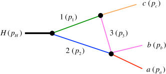
Figure 1: Triangle diagram for $H\to abc$ decay. Particle labels and their momenta (in parentheses) are defined.

Although it was claimed in Refs. Pakhlov2011 ; Pakhlov2015 that an on-shell triangle loop, which includes an experimentally unobserved hadron, can induce a spectrum bump of $Z_{c}(4430)$, the kinematics of the proposed mechanism is in fact classically forbidden and not causing a TS (Coleman-Norton theorem coleman ; also see Fig. 4 and related discussion in Ref. TS-Pc2 ). The mechanism generates a clockwise Argand plot, which is opposite to the LHCb data lhcb_z4430 , and has already been ruled out .

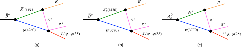
Figure 2: Triangle diagrams contributing to $\bar{B}^{0}\to\psi_{f}K^{-}\pi^{+}$ (a,b) and $\Lambda_{b}^{0}\to\psi_{f}p\pi^{-}$ (c); $\psi_{f}=J/\psi,\psi(2S)$. In (c), $N^{*}$ represents an isospin 1/2 nucleon resonances of 1400$-$1800 MeV. The triangle singularity from the diagram (a) [(b,c)] generates a $Z_{c}(4430)$ [$Z_{c}(4200)$]-like bump in the $\psi_{f}\pi$ invariant mass distribution.

In this paper, we give a new insight into $Z_{c}(4430)$ and $Z_{c}(4200)$ by showing that these exotic candidates can be consistently interpreted as TS if the TS have absolute strengths detectable in the experiments. First we point out that triangle diagrams in Fig. 2, formed by experimentally well-established hadrons, meet the kinematical condition to cause the TS (in the zero width limit of unstable particles). Then we demonstrate that the diagram of Fig. 2(a) [Fig. 2(b,c)] creates a $Z_{c}(4430)$ [$Z_{c}(4200)$]-like bump in the $\psi_{f}\pi$ ($\psi_{f}=J/\psi,\psi(2S)$) invariant mass distribution of $\bar{B}^{0}\to\psi(2S)K^{-}\pi^{+}$ [$\bar{B}^{0}\to J/\psi K^{-}\pi^{+}$ and $\Lambda_{b}^{0}\to J/\psi p\pi^{-}$]. The Breit-Wigner masses and widths fitted to the spectra turn out to be in very good agreement with those of $Z_{c}(4430)$ and $Z_{c}(4200)$. The $Z_{c}(4430)$ Argand plot from the LHCb lhcb_z4430 is also well reproduced by the triangle diagram. Finally, we give a natural explanation for the absence of $Z_{c}(4430)$ in $\Lambda_{b}^{0}\to J/\psi p\pi^{-}$ and $e^{+}e^{-}$ annihilations in terms of the TS. This is so far the most successful TS-based interpretation of charged quarkonium-like states; $Z_{c}(3900)$ as TS has been disfavored in Ref. TS-Zc3900-2  .

First we show that the triangle diagrams in Fig. 2 hit the TS in the zero width limit of the unstable particles. A set of equations presented in Sec. II of Ref. TS-Pc2 is useful for this purpose. Regarding Fig. 2(a), we substitute the PDG averaged particle masses pdg into the formulas, and obtain $p_{1}=p_{2}=491$ MeV, $p_{3}=154$ MeV (the momentum symbols of Fig. 1) in the $\bar{B}^{0}$-at-rest frame, and $m_{\psi(2S)\pi}=4420$ MeV ($\psi(2S)\pi$ invariant mass) at the TS where all particles in the loop have classically allowed energies and momenta. Similarly, we obtain $m_{J/\psi\pi}=4187$ MeV at the TS for Fig. 2(b), and $m_{J/\psi\pi}=3970$ MeV, 4004 MeV, 4116 MeV for Fig. 2(c) with $N^{*}=N(1440)\,1/2^{+}$, $N(1520)\,3/2^{-}$, and $N(1680)\,5/2^{+}$, respectively. In the realistic case where the unstable particles have finite widths, the triangle diagrams do not exactly hit the TS and the location of the spectrum peak due to the TS can be somewhat different from the above $m_{\psi_{f}\pi}$ values. Using the same formulas, we can also confirm that the triangle diagrams of Refs. Pakhlov2011 ; Pakhlov2015 are, in the zero-width limit, kinematically forbidden at the classical level.

We use a simple and reasonable model to calculate the triangle diagrams of Fig. 2. Let us use labeling of particles and their momenta in Fig. 1 to generally express the triangle amplitudes:

$$T_{abc,H} = \int d\bm{p}_{1}\,{v_{ab;23}(\bm{p}_{a},\bm{p}_{b};\bm{p}_{2},\bm{p}_{3})\,\Gamma_{3c,1}(\bm{p}_{3},\bm{p}_{c};\bm{p}_{1})\over E-E_{2}(\bm{p}_{2})-E_{3}(\bm{p}_{3})-E_{c}(\bm{p}_{c})}$$ (1)

$$\times {1\over E-E_{1}(\bm{p}_{1})-E_{2}(\bm{p}_{2})}\Gamma_{12,H}(\bm{p}_{1},\bm{p}_{2};\bm{p}_{H})\ ,$$

where the summation over spin states of the intermediate particles is implied. The quantity $E$ denotes the total energy in the center-of-mass (CM) frame, and $E_{x}(\bm{p}_{x})=\sqrt{\bm{p}^{2}_{x}+m^{2}_{x}}$ is the energy of a particle $x$ with the mass $m_{x}$ and momentum $\bm{p}_{x}$. An exception is applied to unstable intermediate particles 1 and 2 for which $E_{j}(\bm{p}_{j})=m_{j}+\bm{p}^{2}_{j}/2m_{j}-i\Gamma_{j}/2\ (j=1,2)$ where $\Gamma_{j}$ is the width. It is important to consider the vector charmonium width in Fig. 2(a) where $\psi(4260)$ and $K^{*}(892)$ have comparable widths. We use the mass and width values from Ref. pdg .

Regarding the $23\to ab$ interaction $v_{ab;23}$ in Eq. (1), where the particles 2 and $a$ are vector charmoniums while 3 and $b$ are pions, we use an $s$-wave interaction:

$$v_{ab;23}(\bm{p}_{a},\bm{p}_{b};\bm{p}_{2},\bm{p}_{3})=f^{01}_{ab}(p_{ab})f^{01}_{23}(p_{23})\,\bm{\epsilon}^{*}_{a}\cdot\bm{\epsilon}_{2}\ ,$$ (2)

where $\bm{\epsilon}_{a}$ and $\bm{\epsilon}_{2}$ are polarization vectors for the particles $a$ and 2, respectively. The form factors $f^{01}_{ab}(p_{ab})$ and $f^{01}_{23}(p_{23})$ will be defined in Eq. (4); the momentum of the particle $i$ in the $ij$-CM frame is denoted by $\bm{p}_{ij}$ and $p_{ij}=|\bm{p}_{ij}|$. An $s$-wave pair of $\psi_{f}\pi$ coming out from this interaction has $J^{P}=1^{+}$, which is consistent with the experimentally determined spin-parity of $Z_{c}(4430)$ and $Z_{c}(4200)$, and also with the insignificant $d$-wave contribution in the $Z_{c}(4430)$-region lhcb_z4430 .

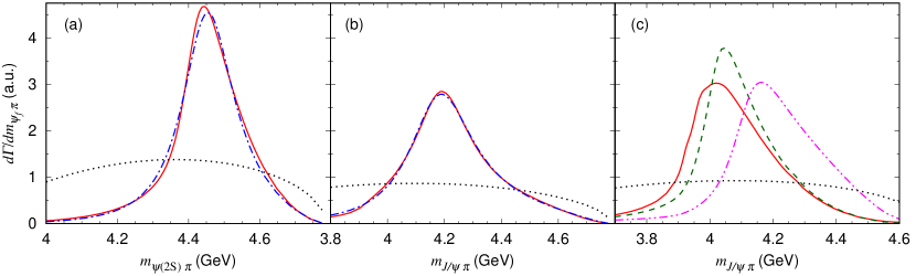
Figure 3: Distributions of the $\psi_{f}\pi$ ($\psi_{f}=J/\psi,\psi(2S)$) invariant mass for $\bar{B}^{0}\to\psi(2S)K^{-}\pi^{+}$ (a), $\bar{B}^{0}\to J/\psi K^{-}\pi^{+}$ (b), and $\Lambda_{b}^{0}\to J/\psi p\pi^{-}$ (c). The red solid curves in panels (a) and (b) are obtained from triangle diagrams Figs. 2(a) and 2(b), respectively. The blue dash-dotted curves are from Breit-Wigner amplitudes fitted to the red solid curves. In panel (c), the red solid, green dashed, and magenta dash-two-dotted curves are obtained from Fig. 2(c) with $N^{*}=N(1440)\,1/2^{+}$, $N(1520)\,3/2^{-}$, and $N(1680)\,5/2^{+}$, respectively. The dotted curves are the phase-space distributions. Each curve, except for the blue dash-dotted ones, is normalized to give unity when integrated with respect to $m_{\psi_{f}\pi}$.

The $R\to ij$ decay vertex $\Gamma_{ij,R}$ in Eq. (1) is explicitly given as

$$\Gamma_{ij,R}(\bm{p}_{i},\bm{p}_{j};\bm{p}_{R}) = \sum_{LS}f^{LS}_{ij}(p_{ij})(s_{i}s_{i}^{z}s_{j}s_{j}^{z}|SS^{z})$$ (3)

$$\times (LMSS^{z}|s_{R}s^{z}_{R})Y_{LM}(\hat{p}_{ij})\ ,$$

where $Y_{LM}$ is spherical harmonics. Clebsch-Gordan coefficients are written as $(abcd|ef)$, and the spin and its $z$-component of a particle $x$ are denoted by $s_{x}$ and $s_{x}^{z}$, respectively. The form factor $f^{LS}_{ij}(p_{ij})$ is parametrized as

$$f^{LS}_{ij}(p)=g^{LS}_{ij}{p^{L}\over\sqrt{E_{i}(p)E_{j}(p)}}\left(\frac{\Lambda^{2}}{\Lambda^{2}+p^{2}}\right)^{2+(L/2)}\ ,$$ (4)

where we use the same cutoff for all the vertices, and set $\Lambda=1$ GeV throughout unless otherwise stated. For each of the $1\to 3c$ and $23\to ab$ interactions, there is only one available set of $\{L,S\}$. We can determine the $g^{LS}_{ij}$ values for the $1\to 3c$ interactions using data such as $\bar{K}^{*}(892)/\bar{K}^{*}_{2}(1430)\to K^{-}\pi^{+}$, and $N^{*}\to\pi^{-}p$ partial decay widths. One might think the $23\to ab$ coupling strength can also be determined using $2\to ab\bar{3}$ ($\bar{3}$: antiparticle of 3) partial decay width. However, the $ab$ invariant mass in the triangle diagram is significantly larger (by   $>$$\sim$   500 MeV) than that of the $2\to ab\bar{3}$ decay process, and thus the coupling strengths may be very different between the two. We leave the $23\to ab$ couplings arbitrary.

The $H\to 12$ decay vertices are currently not well understood because detailed experimental and lattice QCD inputs are lacking. There are still some hints to support the reasonability of considering the $\bar{B}^{0}\to\psi(4260)\bar{K}^{*}(892)$ vertex in Fig. 2(a): (i) the Belle found excess of $B\to\psi(4260)K$ events above the background belle_y4260 ; (ii) the D0’s data can be consistently interpreted that some $b$-flavored hadrons weakly decay into states including $\psi(4260)$ d0_y4260 . Because the details of the $H\to 12$ vertex would not change the main conclusions, we assume simple structures and use arbitrary strengths. Among several sets of $\{L,S\}$ available to the $\bar{B}^{0}$ decays, we set $g^{LS}_{ij}\neq 0$ only for $S=|s_{1}-s_{2}|$ and the lowest allowed $L$; $g^{LS}_{ij}=0$ for the other $\{L,S\}$. Because of using the above $v_{ab;23}$, the $\bar{B}^{0}$ decays are necessarily parity-violating. For the $\Lambda_{b}^{0}$ decays, on the other hand, both parity-conserving and -violating interactions are possible. We choose the parity-conserving one and set $g^{LS}_{ij}\neq 0$ only for $S=|s_{1}-s_{2}|$ and the lowest allowed $L$; $g^{LS}_{ij}=0$ otherwise.

We evaluate the interactions of Eqs. (2) and (3) in the CM frame of the two-body subsystem, and then multiply kinematical factors to account for the Lorentz transformation to the total three-body CM frame; see Appendix C of Ref. 3pi . The procedure of calculating the Dalitz plot distribution for $H\to abc$ using $T_{abc,H}$ of Eq. (1) is detailed in Appendix B of Ref. 3pi .

We first present the $\psi_{f}\pi$ invariant mass distributions for $\bar{B}^{0}\to\psi(2S)K^{-}\pi^{+}$ and $\bar{B}^{0}\to J/\psi K^{-}\pi^{+}$. The red solid curves in Figs. 3(a) and 3(b) are solely from the triangle diagrams of Figs. 2(a) and 2(b), respectively. For comparison, we also plot the phase-space distributions by the black dotted curves. A clear resonance-like peak appears at $m_{\psi(2S)\pi}\sim 4.45$ GeV in Fig. 3(a) ($m_{J/\psi\pi}\sim 4.2$ GeV in Fig. 3(b)) due to the TS. We also calculated the $m_{J/\psi\pi}$ spectrum for $\bar{B}^{0}\to J/\psi K^{-}\pi^{+}$ from the triangle diagram of Fig. 2(a), and obtained a result very similar to Fig. 3(a) after the normalization explained in the caption.

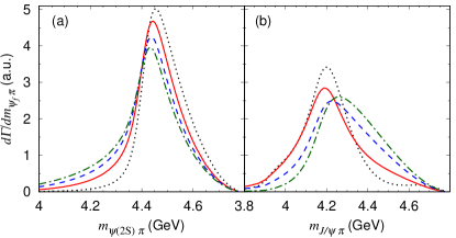
Figure 4: Cutoff dependence of the spectra in Fig. 3. The panels (a) and (b) correspond to Figs. 3(a) and 3(b), respectively. The red solid curves are the same as those in Fig. 3, and are from calculations using the cutoff $\Lambda=1$ GeV. The black dotted, blue dashed, and green dash-dotted curves are obtained with $\Lambda=$ 0.5, 1.5, and 2 GeV, respectively. All the curves are normalized as in Fig. 3.

In an ideal situation where experimental inputs are available to determine all the vertices appearing in the triangle diagrams, we can make a solid prediction of the spectra to be shown in Fig. 3. This is not the case in reality, and thus we examine how the above results depend on the cutoff $\Lambda$ of the form factors in Eq. (4). The spectra in Fig. 4 are obtained by changing the cutoff over a reasonable range: $\Lambda=$ 0.5–2 GeV. The clear peak structures are stable, and the positions and widths of the bumps do not largely change. Therefore, we can conclude that the bump structures in Fig. 3 are essentially determined by the kinematical singularities and are robust in this reasonable cutoff range. The stability of the bumps against changing the cutoff can be explained below. When all particles in the loop have zero widths, the loop momentum exactly hits the TS at a certain $m_{\psi_{f}\pi}$, which blows up the spectrum to infinity irrespective of the cutoff value. The finite widths prevent this from happening and introduce the cutoff dependence to an extent that they push the TS away from the physical region.

We associate the peaks from the TS with fake $Z_{c}$-excitation mechanisms. We fit the Dalitz plot distributions from the triangle diagrams of Figs. 2(a) and 2(b) using the mechanism of $\bar{B}^{0}\to Z_{c}K^{-}$ followed by $Z_{c}\to\psi_{f}\pi^{+}$. The $Z_{c}$ propagation is expressed by the Breit-Wigner form used in Ref. belle_z4430 . The fitting parameters included in the $Z_{c}$-excitation mechanisms are the Breit-Wigner mass, width, and also the cutoff in the form factor of Eq. (4) at the vertices. In the fit, we consider the kinematical region where the magnitude of the Dalitz plot distribution is larger than 10% of the peak height. The obtained fits of reasonable quality are shown by the blue dash-dotted curves in Figs. 3(a) and 3(b). Because the spectrum shape from the triangle diagrams is somewhat different from the Breit-Wigner, their peak positions are slightly different.

Table 1: Breit-Wigner mass (third row) and width (fourth row) for $Z_{c}(4430)$ and $Z_{c}(4200)$; the unit is MeV. $Z_{c}(4430)$ [$Z_{c}(4200)$] parameters are fitted to the Dalitz plot distributions for $\bar{B}^{0}\to\psi(2S)K^{-}\pi^{+}$ (a) [$\bar{B}^{0}\to J/\psi K^{-}\pi^{+}$ (b)] generated by triangle diagram Fig. 2(a) [2(b)]. The ranges are from the cutoff dependence. The parameters from the experimental analyses are also shown; the first (second) errors are statistical (systematic).

$Z_{c}(4430)$			$Z_{c}(4200)$
(a)	Belle belle_z4430	LHCb lhcb_z4430	(b)	Belle belle_z4200
$4463\pm 13$	$4485\pm 22^{+28}_{-11}$	$4475\pm 7^{+15}_{-25}$	$4233\pm 48$	$4196^{+31}_{-29}{}^{+17}_{-13}$
$195\pm 16$	$200^{+41}_{-46}{}^{+26}_{-35}$	$172\pm 13^{+37}_{-34}$	$292\pm 56$	$370\pm 70^{+70}_{-132}$

We fit the Dalitz plot distributions corresponding to different cutoffs of $\Lambda=0.5-2$ GeV (Fig. 4), and present in Table 1 the range of the resulting Breit-Wigner parameters along with those from experimental data. Their agreement is remarkable.

Next we confront the triangle amplitude with the $Z_{c}(4430)$ Argand plot from the LHCb lhcb_z4430 . Because $Z_{c}$ and $K^{-}$ are relatively in $p$-wave, the angle-independent part of the amplitude ($A$) to be compared with the Argand plot is

$$A(m^{2}_{ab})=c_{\rm\,bg}+c_{\rm\,norm}\int d\Omega_{p_{c}}Y^{*}_{1,-s^{z}_{Z_{c}}}(-\hat{p}_{c})M_{abc,H}\ ,$$ (5)

where $s^{z}_{Z_{c}}$ is the $z$-component of the $Z_{c}$ spin and $m_{ab}$ the $ab$ invariant mass. The invariant amplitude $M_{abc,H}$ is related to $T_{abc,H}$ of Eq. (1) through Eq. (B3) of Ref. 3pi . Complex constants $c_{\rm\,norm}$ and $c_{\rm\,bg}$ are adjusted to fit the empirical Argand plot; $c_{\rm\,bg}$ represents a background. In the LHCb analysis, a complex value representing the $Z_{c}(4430)$ amplitude is fitted to dataset in a $m^{2}_{\psi(2S)\pi}$ bin with a bin size $\Delta$. To take account of the bin size, we simply average our amplitude without pursuing a theoretical rigor:

$$\bar{A}(m^{2}_{ab}(i))={1\over\Delta}\int^{m^{2}_{ab}(i)+\Delta/2}_{m^{2}_{ab}(i)-\Delta/2}A(m^{2}_{ab})\,dm^{2}_{ab}\ ,$$ (6)

where $m^{2}_{ab}(i)$ is the central value of an $i$-th bin. As shown in Fig. 5, the empirical $Z_{c}(4430)$ Argand plot is fitted well with $\bar{A}(m^{2}_{ab}(i))$ from the triangle diagram of Fig. 2(a); $c_{\rm\,bg}=0.12+0.03i$ in Eq. (5). This demonstrates that the counterclockwise behavior found in Ref. lhcb_z4430 does not necessarily indicate the existence of a resonance state. Similar statements have also been made for threshold cusps z4430_cusp2 ; TS-Pc .

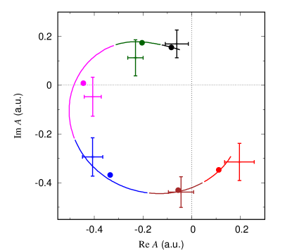
Figure 5: $Z_{c}(4430)$ Argand plot. Six curved segments are from triangle diagram Fig. 2(a). Six data points from Ref. lhcb_z4430 are from fitting data in six bins equally-separating the range of $18~{}{\rm GeV}^{2}\leq m^{2}_{\psi(2S)\pi}\leq 21.5~{}{\rm GeV}^{2}$; $m^{2}_{\psi(2S)\pi}$ increases counterclockwise. A curved segment and a data point of the same color belong to the same bin. A solid circle is an average of the curved segment of the same color. See Eq. (6) for averaging.

We also confirmed a counterclockwise behavior of the Argand plot from the triangle diagram of Fig. 2(b), as the Belle belle_z4200 found the $Z_{c}(4200)$ amplitude to behave so.

A puzzle about $Z_{c}(4430)$ is its large branching to $\psi(2S)\pi$ compared with $J/\psi\pi$: $R^{\rm exp}_{Z_{c}(4430)}\equiv{\cal B}[Z^{+}_{c}(4430)\to\psi(2S)\pi^{+}]/{\cal B}[Z^{+}_{c}(4430)\to J/\psi\pi^{+}]\sim 11$ belle_z4430 ; belle_z4200 . This can be qualitatively understood if $Z_{c}(4430)$ is due to the TS, and the coupling strength ratio ($c^{R}_{\psi\pi}$) of $\psi(4260)\pi^{+}\to\psi(2S)\pi^{+}$ to $\psi(4260)\pi^{+}\to J/\psi\pi^{+}$ interactions of Eq. (2) is fixed by $R^{\rm exp}_{\psi(4260)}\equiv{\cal B}[\psi(4260)\to\psi(2S)\pi^{+}\pi^{-}]/{\cal B}[\psi(4260)\to J/\psi\,\pi^{+}\pi^{-}]=(0.11\pm 0.03\pm 0.03)-(0.55\pm 0.18\pm 0.19)$ from four different solutions of Ref. Y4260-ratio . Because of the large difference in the phase-space available to the final states, $R^{\rm model}_{\psi(4260)}=0.29\times|c^{R}_{\psi\pi}|^{2}$ is obtained by using Eq. (2). In addition, the larger phase-space allows resonance(-like) $f_{0}(980)$ Y4260-f0 and $Z_{c}(3900)$ Y4260-Z3900 to contribute to ${\cal B}[\psi(4260)\to J/\psi\,\pi^{+}\pi^{-}]$ by $\sim 40\%$, and thus $R^{\rm model}_{\psi(4260)}\sim 0.17\times|c^{R}_{\psi\pi}|^{2}$. Therefore, the model reproduces $R^{\rm exp}_{\psi(4260)}\sim 0.54$ with $|c^{R}_{\psi\pi}|\sim 1.8$, and the puzzling $R^{\rm exp}_{Z_{c}(4430)}\sim 11$ is also reproduced with the same $|c^{R}_{\psi\pi}|$. It is however noted that this discussion is based on the assumption that $c^{R}_{\psi\pi}$ is the same for the $\psi(4260)\pi^{+}$ scattering at the TS and the $\psi(4260)$ decays. As discussed earlier, these two processes are significantly different in the energy, and thus $c^{R}_{\psi\pi}$ is not necessarily the same.

Now we discuss the $J/\psi\pi$ invariant mass distribution for $\Lambda_{b}^{0}\to J/\psi p\pi^{-}$ induced by the triangle diagram of Fig. 2(c). In the $Z_{c}(4200)$-region, the TS is expected to create a spectrum bump. Interestingly, several isospin 1/2 nucleon resonances ($N^{*}$) of 1400$-$1800 MeV can contribute to the singularities and, depending on the mass and width of $N^{*}$, the position and width of the bump can vary. In Fig. 3(c), we show results obtained with some representative four-star resonances: $N^{*}=N(1440)\,1/2^{+}$, $N(1520)\,3/2^{-}$, and $N(1680)\,5/2^{+}$. As expected, the triangle diagrams including different $N^{*}$ generate different spectrum bumps in the $Z_{c}(4200)$-region. In reality, these bumps may coherently interfere with each other to create a single broad bump. Also, other charmoniums of 3650-3900 MeV with coupling to $J/\psi\pi\pi$, such as $\psi(2S)$ and $\chi_{c1}(3872)$, could replace $\psi(3770)$ in Fig. 2(c) to generate TS bumps in the $Z_{c}(4200)$-region. The LHCb analysis lhcb_z4200_Lb found that the $\Lambda_{b}^{0}\to J/\psi p\pi^{-}$ decay data is significantly better described by including the $Z_{c}(4200)$ amplitude. Because of limited statistics, the mass and width of $Z_{c}(4200)$ were assumed to be the same as those in $\bar{B}^{0}\to J/\psi K^{-}\pi^{+}$ belle_z4200 . Therefore, the spectrum bumps shown in Fig. 3(c), some of which extend to the lower end of the $Z_{c}(4200)$-region, are still consistent with the LHCb’s finding.

Another important finding in the LHCb analysis lhcb_z4200_Lb is that $Z_{c}(4430)$ seems to hardly contribute to $\Lambda_{b}^{0}\to J/\psi p\pi^{-}$. If $Z_{c}(4430)$ found in $\bar{B}^{0}\to\psi(2S)K^{-}\pi^{+}$ is due to the TS, a natural explanation follows: within experimentally observed hadrons, no combination of a charmonium and a nucleon resonance is available to form a triangle diagram like Fig. 2(c) that causes TS at the $Z_{c}(4430)$ position. This idea can be further generalized. At present, a puzzling situation about $Z_{c}$ is that those observed in $e^{+}e^{-}$ annihilations and in $B$ decays are mutually exclusive. If the $Z_{c}$ states are due to TSs, the answer is simple: a TS in a $B$ decay does not exist or is highly suppressed in $e^{+}e^{-}$ annihilations, and vice versa. Therefore, a key to establishing a genuine tetraquark state is to identify it in different processes including different initial states. However, there are still cases where, as we have seen in Figs. 3(b) and 3(c), different TS could induce similar resonance-like behaviors.

In summary, we demonstrated that $Z_{c}(4430)$ and $Z_{c}(4200)$, which are often regarded as genuine tetraquark states, can be consistently interpreted as kinematical singularities from the triangle diagrams we identified. The Breit-Wigner parameters fitted to the TS-induced spectrum bumps of $\bar{B}^{0}\to\psi_{f}K^{-}\pi^{+}$ are in very good agreement with those of $Z_{c}(4430)$ and $Z_{c}(4200)$ from the Belle and LHCb analyses. The $Z_{c}(4430)$ Argand plot from the LHCb is also well reproduced. We also explained in terms of TS why $Z_{c}(4200)$-like contribution was observed in $\Lambda_{b}^{0}\to J/\psi p\pi^{-}$ but $Z_{c}(4430)$ was not. These results are robust because they are essentially determined by the kinematical effect, and not sensitive to uncertainty of dynamical details.

- (1) M. Tanabashi et al. (Particle Data Group), Phys. Rev. D 98, 030001 (2018).
- (2) S.K. Choi et al. (Belle Collaboration), Phys. Rev. Lett. 100, 142001 (2008).
- (3) L. Maiani, F. Piccinini, A.D. Polosa, and V. Riquer, Phys. Rev. D 89, 114010 (2014).
- (4) D. Ebert, R.N. Faustov, and V.O. Galkin, Eur. Phys. J. C 58, 399 (2008).
- (5) C. Deng, J. Ping, H. Huang, and F. Wang, Phys. Rev. D 92, 034027 (2015).
- (6) X. Liu, Y.-R. Liu, W.-Z. Deng, and S.-L. Zhu Phys. Rev. D 77, 034003 (2008).
- (7) G.-J. Ding, W. Huang, J.-F. Liu, and M.-L. Yan, Phys. Rev. D 79, 034026 (2009).
- (8) S.H. Lee, A. Mihara, F.S. Navarra, and M. Nielsen, Phys. Lett. B 661, 28 (2008).
- (9) J.-R. Zhang and M.-Q. Huang, Phys. Rev. D 80, 056004 (2009).
- (10) L. Ma, X.-H. Liu, X. Liu, and S.-L. Zhu, Phys. Rev. D 90, 037502 (2014).
- (11) J.L. Rosner, Phys. Rev. D 76, 114002 (2007).
- (12) D.V. Bugg, J. Phys. G 35, 075005 (2008).
- (13) A. Hosaka, T. Iijima, K. Miyabayashi, Y. Sakai, and S. Yasui, Prog. Theor. Exp. Phys. 2016, 062C01 (2016).
- (14) H.-X. Chen, W. Chen, X. Liu, and S.-L. Zhu, Phys. Rept. 639, 1 (2016).
- (15) R.F. Lebed, R.E. Mitchell, and E.S. Swanson, Prog. Part. Nucl. Phys. 93, 143 (2017).
- (16) R.M. Albuquerque, J.M. Dias, K.P. Khemchandani, A. Martinez Torres, F.S. Navarra, M. Nielsen, and C.M. Zanetti, J. Phys. G 46, 093002 (2019).
- (17) K. Chilikin et al. (Belle Collaboration), Phys. Rev. D 88, 074026 (2013).
- (18) R. Aaij et al. (LHCb Collaboration), Phys. Rev. Lett. 112, 222002 (2014).
- (19) https://physics.aps.org/synopsis-for/10.1103/PhysRevLett.112.222002
- (20) W. Chen, T.G. Steele, H.-X. Chen, and S.-L. Zhu, Eur. Phys. J. C 75, 358 (2015).
- (21) K. Chilikin et al. (Belle Collaboration), Phys. Rev. D 90, 112009 (2014).
- (22) R. Aaij et al. (LHCb collaboration), Phys. Rev. Lett. 122, 152002 (2019).
- (23) R. Aaij et al. (LHCb Collaboration), Phys. Rev. Lett. 117, 082003 (2016).
- (24) L.D. Landau, Nucl. Phys. 13, 181 (1959).
- (25) I.J.R. Aitchison, Phys. Rev. 133, B1257 (1964).
- (26) S. Coleman and R.E. Norton, Nuovo Cimento 38, 438 (1965).
- (27) C. Schmid, Phys. Rev. 154, 1363 (1967).
- (28) R. J. Eden, P. V. Landshoff, D. I. Olive and J. C. Polkinghorne, The Analytic S-Matrix, (Cambridge University Press, Cambridge, England, 1966).
- (29) F.-K. Guo, U.-G. Meißner, W. Wang, and Z. Yang, Phys. Rev. D 92, 071502(R) (2015).
- (30) X.-H. Liu, Q. Wang, and Q. Zhao, Phys. Lett. B757, 231 (2016).
- (31) M. Bayar, F. Aceti, F.-K. Guo, and E. Oset, Phys. Rev. D 94, 074039 (2016).
- (32) A. Pilloni, C. Fernandez-Ramirez, A. Jackura, V. Mathieu, M. Mikhasenko, J. Nys, and A.P. Szczepaniak, Phys. Lett. B 772, 200 (2017).
- (33) Q.-R. Gong, J.-L. Pang, Y.-F. Wang, and H.-Q. Zheng Eur. Phys. J. C 78, 276 (2018).
- (34) A.P. Szczepaniak, Phys. Lett. B 747, 410 (2015).
- (35) P. Pakhlov, Phys. Lett. B702, 139 (2011).
- (36) P. Pakhlov and T. Uglov, Phys. Lett. B748, 183 (2015).
- (37) R. Aaij et al. (LHCb Collaboration), Phys. Rev. Lett. 122, 222001 (2019).
- (38) R. Garg et al. (Belle collaboration), Phys. Rev. D 99, 071102(R) (2019).
- (39) V.M. Abazov et al. (D0 Collaboration), Phys. Rev. D 100, 012005 (2019).
- (40) H. Kamano, S.X. Nakamura, T.-S.H. Lee, and T. Sato, Phys. Rev. D 84, 114019 (2011).
- (41) J. Zhang and L. Yuan, Eur. Phys. J. C 77, 727 (2017).
- (42) J.P. Lees et al. (BaBar Collaboration), Phys. Rev. D 86, 051102(R) (2012).
- (43) M. Ablikim et al. (BESIII Collaboration), Phys. Rev. Lett. 110, 252001 (2013).