Could the near–threshold $XYZ$ states be simply kinematic effects?

Abstract

We demonstrate that the spectacular structures discovered recently in various experiments and named as $X$, $Y$ and $Z$ states cannot be purely kinematic effects. Their existence necessarily calls for nearby poles in the $S$–matrix and they therefore qualify as states. We propose a way to distinguishing kinematic cusp effects from genuine $S$–matrix poles: the kinematic threshold cusp cannot produce a narrow peak in the invariant mass distribution in the elastic channel in contrast with a genuine $S$–matrix pole.

In recent years various narrow (widths from well below 100 MeV down to values even below 1 MeV) peaks were discovered both in the charmonium as well as in the bottomonium mass range that do not fit into the so far very successful quark model. For instance, the most prominent ones include $X(3872)$ Choi:2003ue , $Z_{c}(3900)$ Ablikim:2013mio ; Liu:2013dau ; Xiao:2013iha , $Z_{c}(4020)$ Ablikim:2013xfr ; Ablikim:2013wzq ; Ablikim:2013emm ; Ablikim:2014dxl , $Z_{b}(10610)$ and $Z_{b}(10650)$ Belle:2011aa , which are located close to $D\bar{D}^{*}$, $D\bar{D}^{*}$, $D^{*}\bar{D}^{*}$, $B\bar{B}^{*}$ and $B^{*}\bar{B}^{*}$ thresholds in relative $S$–waves, respectively. Apart from other interpretations, such as hadro-quarkonia Voloshin:2007dx ; Dubynskiy:2008mq , hybrids Zhu:2005hp ; Kou:2005gt ; Close:2005iz , and tetraquarks Maiani:2014aja ; Faccini:2013lda (for recent reviews we refer to Refs. Brambilla:2010cs ; italians ), due to their proximity to the thresholds these five states were proposed to be of a molecular nature Tornqvist:2004qy ; Fleming:2007rp ; Thomas:2008ja ; Ding:2008gr ; Lee:2009hy ; Dong:2009yp ; Stapleton:2009ey ; Gamermann:2009fv ; Mehen:2011ds ; Bondar:2011ev ; Nieves:2011vw ; Nieves:2012tt ; Wang:2013cya ; Wang:2013kra ; Guo:2013sya ; Guo:2013zbw ; Mehen:2013mva ; He:2013nwa ; Liu:2014eka . As an alternative explanation various groups conclude from the mentioned proximity of the states to the thresholds that the structures are simply kinematical effects Bugg:2004rk ; Bugg:2011jr ; Chen:2011pv ; Chen:2011xk ; Chen:2011pu ; Chen:2013coa ; Chen:2013wca ; Swanson:2014tra that necessarily occur near every $S$-wave threshold. Especially, it has been claimed that the structures are not related to a pole in the $S$–matrix and therefore should not be interpreted as states.

In this letter we show that the latter statement is based on calculations performed within an inconsistent formalism. In particular, we demonstrate that, while there is always a cusp at the opening of an $S$–wave threshold, in order to produce peaks as pronounced and narrow as observed in experiment non-perturbative interactions amongst the heavy mesons are necessary, and as a consequence, there is to be a near-by pole. Or, formulated the other way around: if one assumes the two–particle interactions to be perturbative, as it is implicitly done in Refs. Bugg:2004rk ; Bugg:2011jr ; Chen:2011pv ; Chen:2011xk ; Chen:2011pu ; Chen:2013coa ; Chen:2013wca ; Swanson:2014tra , the cusp should not appear as a prominent narrow peak. This statement is probably best illustrated by the famous $K^{\pm}\to\pi^{\pm}\pi^{0}\pi^{0}$ data Batley:2000zz : the cusp that appears in the $\pi^{0}\pi^{0}$ invariant mass distribution at the $\pi^{+}\pi^{-}$ threshold is a very moderate kink, since the $\pi\pi$ interactions are sufficiently weak to allow for a perturbative treatment (for a comprehensive theoretical framework and related references we refer to Ref. Gasser:2011ju ).

Figure 1: The tree-level, one-loop and two-loop Feynman diagrams for $Y(4260)\to\pi D\bar{D}^{*}$.

To be concrete, in this paper we demonstrate our argument on the example of an analysis of the existing data on the $Z_{c}(3900)$, but it should be clear that the reasoning as such is general and applies to all structures observed very near $S$–wave thresholds such as those above-mentioned $XYZ$ states. To illustrate our point, we here do not aim for field theoretical rigor but use a very simple separable interaction for all vertices accompanied by loops regularized with a Gaussian regulator. This regulator will at the same time control the drop-off of the amplitudes as will be discussed below. Accordingly, we write for the Lagrangian that produces the tree–level vertices (here and in what follows we generically write $D\bar{D}^{*}$ for the proper linear combination of $D\bar{D}^{*}$ and $\bar{D}D^{*}$)

$${\cal L}_{I} = g_{Y}\pi(D\bar{D}^{*}_{\mu})^{\dagger}Y^{\mu}+\frac{C}{2}(D\bar{D}^{*})^{\dagger}(D\bar{D}^{*})$$ (1)

$$\quad+\,g_{\psi Y}\psi^{\mu\dagger}\pi\pi Y_{\mu}+g_{\psi}\psi^{\mu\dagger}\pi D\bar{D}^{*}_{\mu}+...\ ,$$

where $Y$, $D$, $D^{*}$, $\pi$ and $\psi$ denote the fields for the $Y(4260)$, $D$, $D^{*}$, $\pi$ and $J/\psi$, respectively. The dots indicate terms not needed for this study like the one where the $Y$-field is created. All fields but the pion field are nonrelativistic and accordingly the couplings $g_{Y}$ and $g_{\psi}$ have dimension GeV^-3/2, $g_{\psi Y}$ has dimension GeV^-1, while $C$ has dimension GeV^-2. The loops are regularized with the cutoff function $f_{\Lambda}(\vec{p}\,^{2})$, which for convenience we choose as

$$f_{\Lambda}(\vec{p}\,^{2})=\exp\left(-2\vec{p}\,^{2}/\Lambda^{2}\right)\ ,$$ (2)

where here and below $\vec{p}$ denotes the three-momentum of the $D$-meson in the center-of-mass frame of the $D\bar{D}^{*}$ system. Therefore the loop function reads

$$G_{\Lambda}(E)=\int\frac{d^{3}q}{(2\pi)^{3}}\frac{f_{\Lambda}(\vec{q}\,^{2})}{E-m_{1}-m_{2}-\vec{q}\,^{2}/(2\mu)}\ ,$$ (3)

where $m_{1,2}$ denote the masses of the charmed mesons, $\mu$ is the reduced mass and $E$ is the total energy. With the regulator specified in Eq. (2), the analytic expression for the loop function for $E\geq m_{1}+m_{2}$ is given by

$$G_{\Lambda}(E)=-\frac{\mu\Lambda}{(2\pi)^{3/2}}+\frac{\mu k}{2\pi}e^{-2k^{2}/\Lambda^{2}}\left[\text{erfi}\left(\frac{\sqrt{2}k}{\Lambda}\right)-i\right],$$ (4)

where $k=\sqrt{2\mu(E-m_{1}-m_{2})}$, and

$$\text{erfi}(z)=\frac{2}{\sqrt{\pi}}\int_{0}^{z}e^{t^{2}}dt$$ (5)

is the imaginary error function.

With the ingredients of the model fixed it is straightforward to derive the explicit expressions for the transition matrix elements. Within this model the $Y(4260)\to\pi D\bar{D}^{*}$ amplitude reads to one-loop order ($cf$. the diagrams of Fig. 1 (a)+(b))

$$g_{Y}\left[1-G_{\Lambda}(E)C\right]\ .$$ (6)

The analogous result for the $Y(4260)\to\pi\pi J/\psi$ amplitude is ($cf$. the diagrams of Fig. 2 (a)+(b))

$$g_{\psi Y}-g_{Y}G_{\Lambda}(E)g_{\psi}\ .$$ (7)

We now proceed as follows: We first confirm the claims of Refs. Bugg:2011jr ; Chen:2013coa ; Swanson:2014tra , namely, that the data available for both $Y(4260)\to\pi D\bar{D}^{*}$ as well as $Y(4260)\to\pi\pi J/\psi$ can at least qualitatively be described by a sum of the tree-level and one–loop diagrams shown in Fig. 1 (a)+(b) and Fig. 2 (a)+(b), respectively. Note that diagram (b) in either Fig. 1 or 2 explicitly contains the above mentioned cusp. It was this observation that lead the authors of Refs. Bugg:2011jr ; Chen:2013coa ; Swanson:2014tra to interpret the near–threshold structures as purely kinematical effect. To fix the parameters we first fix $g_{Y}$, $\Lambda$ and $C$ by a fit to the $D\bar{D}^{*}$ spectrum. The fit result is shown by the solid line in Fig. 3 (the corresponding strength of the tree level diagram is shown by the dotted line). In particular we find

$$C=64.4~{}\text{GeV}^{-2},\quad\Lambda=0.326~{}\text{GeV}$$ (8)

and $g_{Y}=102.6$ GeV^-3/2 (notice that this parameter is not normalized to the physical value since we are fitting to the number of events, and a factor of $\sqrt{8m_{Y}m_{D}m_{D^{*}}}$ needs to be multiplied to it in order to obtain the solid curve shown in Fig. 3) for the best fit. It is crucial for the reasoning of this letter that the contribution from the tree–level source term ($cf$. Fig. 1(a)) and the $D\bar{D}^{*}$ rescattering ($cf$. Fig. 1(b)) can be disentangled, since the former is fixed by the $D\bar{D}^{*}$ spectrum for values of $m_{D\bar{D}^{*}}$ above around 3.94 GeV, while the latter is to explain the structure for values below this invariant mass, see Fig. 3.

Next we keep $g_{Y}$ and $\Lambda$ fixed and fit $g_{\psi}$ and $g_{\psi Y}$ to the $J/\psi\pi$ spectrum. The best fit gives $g_{\psi Y}=46.4$ GeV^-3/2 and $g_{\psi}=0.44$ GeV^-3/2 which are also not normalized to the physical values due to fitting to the event numbers. The result of this fit is shown as the solid line in Fig. 4. In this work we only aim at a qualitative description of the data. It should be mentioned that we can get a perfect fit of the $J/\psi\pi$ spectrum, if we also fit $\Lambda$, but then we have to compromise on the fit quality for the $D\bar{D}^{*}$ channel. Since this fitting procedure leads us to the same conclusions we do not show the corresponding fit results.

Figure 2: The tree-level, one-loop and two-loop Feynman diagrams for $Y(4260)\to\pi\pi J/\psi$.

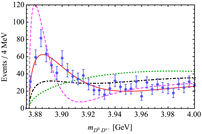
Figure 3: Results for the $D\bar{D}^{*}$ invariant mass distribution in $Y(4260)\to\pi D\bar{D}^{*}$. The data are from Ref. Ablikim:2013xfr and the results from the tree level, full one-loop and full two-loop calculations are shown by the dotted, solid and dashed curves, respectively. The dot–dashed line shows the one-loop result with the strength of the rescattering requested to be small to justify a perturbative treatment as described in the text.

As mentioned above, the intrinsic assumption of the approaches outlined in Refs. Bugg:2011jr ; Chen:2013coa ; Swanson:2014tra is that the interactions are perturbative, and consequently, the amplitude is properly represented by the one loop result. With the parameters fixed we can now calculate the amplitudes to two–loop order from

$$g_{Y}\left[1-G_{\Lambda}(E)C+(G_{\Lambda}(E)C)^{2}\right]\ ,$$ (9)

for the $\pi D\bar{D}^{*}$ channel ($cf$. Fig. 1 (a)+(b)+(c)) and

$$g_{\psi Y}-g_{Y}G_{\Lambda}(E)g_{\psi}+g_{y}G_{\Lambda}(E)CG_{\Lambda}(E)g_{\psi}\$$ (10)

for the $\pi\pi J/\psi$ channel ($cf$. Fig. 2 (a)+(b)+(c)). The results are shown as the dashed lines in Figs. 3 and 4, respectively. As one can see, in both cases the two-loop result significantly deviates from the one-loop result around the peak, which clearly calls for a resummation of the series.

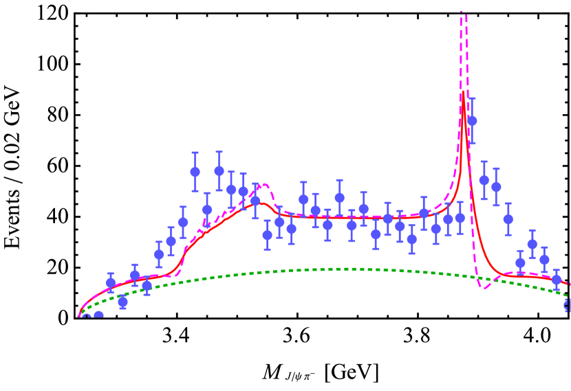
Figure 4: Results for the $\pi J/\psi$ invariant mass distribution in $Y(4260)\to\pi\pi J/\psi$. The data are from Ref. Ablikim:2013mio and the results from the tree level, full one-loop and full two-loop calculations are shown by the dotted, solid and dashed curves, respectively, with the cutoff as well as $g_{Y}$ from the fit to the $D\bar{D}^{*}$ spectrum.

In fact, when we sum all loops in the $D\bar{D}^{*}$ channel using the parameters of Eqs. (8), the series produces a bound state pole right below threshold.  This means the following for the results of Refs. Bugg:2011jr ; Chen:2013coa ; Swanson:2014tra : if one wants to fit the available data for the near-threshold $Z_{c}(3900)$ states within a perturbative approach, the presence of a pronounced near-threshold structure calls for such a large coupling constant that the use of a perturbative approach is not justified. This demonstrates explicitly that the approach used in Refs. Bugg:2011jr ; Chen:2013coa ; Swanson:2014tra is intrinsically inconsistent.

This argument also works in the other direction: we may constrain the coupling $C$ for $D\bar{D}^{*}$ elastic scattering to a value where it might still be justified to treat $D\bar{D}^{*}$ scattering perturbative, e.g. one may require in the full kinematic regime $|G_{\Lambda}(E)C|\ll 1$. Since $|G_{\Lambda}(E)|$ is maximal for $E=2M$, we may demand $|C\,G_{\Lambda}(m_{1}+m_{2})|=a$ with $a\ll 1$. For $\Lambda$ as given in Eq. (8) and $a=1/2$ we can again calculate the amplitude to one–loop order. The resulting $D\bar{D}^{*}$ spectrum is shown by the dot–dashed line in Fig. 3. Clearly, such a small coupling is not able to produce the pronounced structure in the data.

In the calculation described above we used a Gaussian form factor to regularize the loop. We checked that a different regulator leads to qualitatively similar results. Especially the conclusions stay unchanged. In fact, any other form factor which is commonly used drops off more slowly for higher momenta. As a result an even larger value of $|C\,G_{\Lambda}(m_{1}+m_{2})|$ will be connected to a narrow near–threshold structure. From this point of view, the use of a Gaussian form factor as employed above already leads to the most conservative estimate of the higher loop effects. We should also mention that the contact interaction and the regularized loop function always appear in a product, i.e. $G_{\Lambda}(E)C$, so that the momentum dependence introduced in the cut-off function can be equivalently regarded as momentum dependence in the interaction.

To distinguish an $S$–matrix pole from a simple cusp effect it is necessary to fix the strength of the production vertex and of the meson–meson rescattering separately. This is possible only for the elastic channel, as can be clearly seen from comparing Eqs. (6) and (7): the term $CG_{\Lambda}(E)$ which controls the elastic interaction strength can be fixed from the peak since it interferes with 1, while the inelastic coupling strength $g_{\psi}$ in Eq. (7) always appears in a product with $g_{Y}$. We therefore strongly urge all groups claiming a purely kinematic origin of some near threshold structure to also calculate the transition of that structure into the corresponding continuum channel and follow the steps of this paper to either confirm or disprove their claim.

One may wonder if triangle singularities are capable to circumvent the argument presented in this paper. After all they are in principle able to provide enhancements in observables as demonstrated in a different context, e.g. in Refs. Wu:2011yx ; Wu:2012pg (for a recent discussion see Ref. Szczepaniak:2015eza ). However, this mechanism is effective only in a very limited kinematic regime and therefore operative only for selected transitions. Therefore, the very fact that e.g. the $X(3872)$ is seen, amongst others, in $B\to KX$ and $Y(4260)\to\gamma X$ is a clear indication that its existence is not exclusively driven by a triangle singularity. For the case of the $Z_{c}(3900)$ the dependence of the triangle singularity on the external energies is discussed in Ref. Wang:2013hga . Probably even more important for the line of reasoning in this paper, for the elastic channel, i.e. when the incoming and outgoing particles in the final state interaction as part of the triangle diagram are the same, the triangle singularity will not produce any peak Schmid:1967 ; Anisovich:1995ab . Thus, our conclusion which relies mainly on the analysis in the elastic (continuum) channel remains: pronounced, narrow near-threshold peaks cannot be produced by purely kinematic effects.

Although in this work all calculations are tuned to the production of the $Z_{c}(3900)$ seen in $Y(4260)\to\pi Z_{c}(3900)$ it should be understood that the arguments are indeed very general: any consistent treatment of the spectacular very near-threshold structures, namely some of those $XYZ$ states, necessarily needs the inclusion of a nearby pole, which was done, e.g., in Refs. Voloshin:2007dx ; Dubynskiy:2008mq ; Zhu:2005hp ; Kou:2005gt ; Close:2005iz ; Maiani:2014aja ; Faccini:2013lda ; Tornqvist:2004qy ; Fleming:2007rp ; Thomas:2008ja ; Ding:2008gr ; Lee:2009hy ; Dong:2009yp ; Stapleton:2009ey ; Gamermann:2009fv ; Mehen:2011ds ; Bondar:2011ev ; Nieves:2011vw ; Nieves:2012tt ; Wang:2013cya ; Wang:2013kra ; Guo:2013sya ; Guo:2013zbw ; Mehen:2013mva ; He:2013nwa ; Liu:2014eka ; Danilkin:2011sh . For each individual state a detailed high–quality fit to the data is necessary to decide if this pole is located on the first sheet (bound state) or on the second sheet (virtual state or resonance). It also requires additional research to decide on the origin of that pole, which might, e.g., come from short–ranged four–quark interactions or from meson–meson interactions. All we can conclude from the results of this paper is that there has to be a near–threshold pole.

We are grateful for the inspiring atmosphere at the Quarkonium Working Group Workshop 2014 where the idea for this work was born as well as to very useful discussions with Eric Braaten, Estia Eichten, Tom Mehen, Ulf-G. Meißner and Eric Swanson. This work is supported, in part, by NSFC and DFG through funds provided to the Sino-Germen CRC 110 “Symmetries and the Emergence of Structure in QCD” (NSFC Grant No. 11261130311), NSFC (Grant Nos. 11035006 and 11165005), the Chinese Academy of Sciences (KJCX3-SYW-N2), and the Ministry of Science and Technology of China (2015CB856700).

References

- (1) S. K. Choi et al. [Belle Collaboration], Phys. Rev. Lett. 91, 262001 (2003) [hep-ex/0309032].
- (2) M. Ablikim et al. [BESIII Collaboration], Phys. Rev. Lett. 110, 252001 (2013) [arXiv:1303.5949 [hep-ex]].
- (3) Z. Q. Liu et al. [Belle Collaboration], Phys. Rev. Lett. 110, 252002 (2013)
- (4) T. Xiao, S. Dobbs, A. Tomaradze and K. K. Seth, Phys. Lett. B 727, 366 (2013) [arXiv:1304.3036 [hep-ex]].
- (5) M. Ablikim et al. [BESIII Collaboration], Phys. Rev. Lett. 112, 022001 (2014) [arXiv:1310.1163 [hep-ex]].
- (6) M. Ablikim et al. [BESIII Collaboration], Phys. Rev. Lett. 111, 242001 (2013) [arXiv:1309.1896 [hep-ex]].
- (7) M. Ablikim et al. [BESIII Collaboration], arXiv:1308.2760 [hep-ex].
- (8) M. Ablikim et al. [BESIII Collaboration], arXiv:1409.6577 [hep-ex].
- (9) A. Bondar et al. [Belle Collaboration], Phys. Rev. Lett. 108, 122001 (2012) [arXiv:1110.2251 [hep-ex]].
- (10) M. B. Voloshin, Prog. Part. Nucl. Phys. 61, 455 (2008).
- (11) S. Dubynskiy and M. B. Voloshin, Phys. Lett. B 666, 344 (2008).
- (12) S.-L. Zhu, Phys. Lett. B 625, 212 (2005).
- (13) E. Kou and O. Pene, Phys. Lett. B 631, 164 (2005).
- (14) F. E. Close and P. R. Page, Phys. Lett. B 628, 215 (2005).
- (15) L. Maiani, F. Piccinini, A. D. Polosa and V. Riquer, Phys. Rev. D 89, 114010 (2014) [arXiv:1405.1551 [hep-ph]].
- (16) L. Maiani, V. Riquer, R. Faccini, F. Piccinini, A. Pilloni and A. D. Polosa, Phys. Rev. D 87, no. 11, 111102 (2013) [arXiv:1303.6857 [hep-ph]].
- (17) N. Brambilla, S. Eidelman, B. K. Heltsley, R. Vogt, G. T. Bodwin, E. Eichten, A. D. Frawley and A. B. Meyer et al., Eur. Phys. J. C 71, 1534 (2011) [arXiv:1010.5827 [hep-ph]].
- (18) R. Faccini, A. Pilloni and A. D. Polosa, Mod. Phys. Lett. A 27 (2012) 1230025
- (19) N. A. Törnqvist, Phys. Lett. B 590, 209 (2004) [hep-ph/0402237].
- (20) S. Fleming, M. Kusunoki, T. Mehen and U. van Kolck, Phys. Rev. D 76, 034006 (2007) [hep-ph/0703168].
- (21) C. E. Thomas and F. E. Close, Phys. Rev. D 78, 034007 (2008) [arXiv:0805.3653 [hep-ph]].
- (22) G.-J. Ding, Phys. Rev. D 79, 014001 (2009).
- (23) I. W. Lee, A. Faessler, T. Gutsche and V. E. Lyubovitskij, Phys. Rev. D 80, 094005 (2009) [arXiv:0910.1009 [hep-ph]].
- (24) Y. Dong, A. Faessler, T. Gutsche, S. Kovalenko and V. E. Lyubovitskij, Phys. Rev. D 79, 094013 (2009) [arXiv:0903.5416 [hep-ph]].
- (25) E. Braaten and J. Stapleton, Phys. Rev. D 81, 014019 (2010) [arXiv:0907.3167 [hep-ph]].
- (26) D. Gamermann and E. Oset, Phys. Rev. D 80, 014003 (2009) [arXiv:0905.0402 [hep-ph]].
- (27) Q. Wang, C. Hanhart and Q. Zhao, Phys. Rev. Lett. 111, 132003 (2013).
- (28) Q. Wang, M. Cleven, F.-K. Guo, C. Hanhart, U.-G. Meißner, X. -G. Wu and Q. Zhao, Phys. Rev. D 89, 034001 (2014) [arXiv:1309.4303 [hep-ph]].
- (29) T. Mehen and R. Springer, Phys. Rev. D 83, 094009 (2011) [arXiv:1101.5175 [hep-ph]].
- (30) A. E. Bondar, A. Garmash, A. I. Milstein, R. Mizuk and M. B. Voloshin, Phys. Rev. D 84, 054010 (2011) [arXiv:1105.4473 [hep-ph]].
- (31) J. Nieves and M. P. Valderrama, Phys. Rev. D 84, 056015 (2011) [arXiv:1106.0600 [hep-ph]].
- (32) J. Nieves and M. P. Valderrama, Phys. Rev. D 86, 056004 (2012) [arXiv:1204.2790 [hep-ph]].
- (33) F.-K. Guo, C. Hidalgo-Duque, J. Nieves and M. P. Valderrama, Phys. Rev. D 88, 054007 (2013) [arXiv:1303.6608 [hep-ph]].
- (34) F.-K. Guo, C. Hanhart, U.-G. Meißner, Q. Wang and Q. Zhao, Phys. Lett. B 725, 127 (2013) [arXiv:1306.3096 [hep-ph]].
- (35) T. Mehen and J. Powell, Phys. Rev. D 88, 034017 (2013) [arXiv:1306.5459 [hep-ph]].
- (36) J. He, X. Liu, Z. F. Sun and S. L. Zhu, Eur. Phys. J. C 73, 2635 (2013) [arXiv:1308.2999 [hep-ph]].
- (37) X. H. Liu, L. Ma, L. P. Sun, X. Liu and S. L. Zhu, Phys. Rev. D 90, 074020 (2014) [arXiv:1407.3684 [hep-ph]].
- (38) D. V. Bugg, Phys. Lett. B 598, 8 (2004) [hep-ph/0406293].
- (39) D. V. Bugg, Europhys. Lett. 96, 11002 (2011) [arXiv:1105.5492 [hep-ph]].
- (40) D. Y. Chen and X. Liu, Phys. Rev. D 84, 094003 (2011) [arXiv:1106.3798 [hep-ph]].
- (41) D. Y. Chen and X. Liu, Phys. Rev. D 84, 034032 (2011) [arXiv:1106.5290 [hep-ph]].
- (42) D. Y. Chen, X. Liu and T. Matsuki, Phys. Rev. D 84, 074032 (2011) [arXiv:1108.4458 [hep-ph]].
- (43) D. Y. Chen, X. Liu and T. Matsuki, Phys. Rev. D 88, 036008 (2013) [arXiv:1304.5845 [hep-ph]].
- (44) D. Y. Chen, X. Liu and T. Matsuki, Phys. Rev. Lett. 110, 232001 (2013) [arXiv:1303.6842 [hep-ph]].
- (45) E. S. Swanson, arXiv:1409.3291 [hep-ph].
- (46) J. R. Batley, A. J. Culling, G. Kalmus, C. Lazzeroni, D. J. Munday, M. W. Slater, S. A. Wotton and R. Arcidiacono et al., Eur. Phys. J. C 64, 589 (2009) [arXiv:0912.2165 [hep-ex]].
- (47) J. Gasser, B. Kubis and A. Rusetsky, Nucl. Phys. B 850, 96 (2011) [arXiv:1103.4273 [hep-ph]].
- (48) J. J. Wu, X. H. Liu, Q. Zhao and B. S. Zou, Phys. Rev. Lett. 108, 081803 (2012) [arXiv:1108.3772 [hep-ph]].
- (49) X. G. Wu, J. J. Wu, Q. Zhao and B. S. Zou, Phys. Rev. D 87, 014023 (2013) [arXiv:1211.2148 [hep-ph]].
- (50) A. P. Szczepaniak, arXiv:1501.01691 [hep-ph].
- (51) Q. Wang, C. Hanhart and Q. Zhao, Phys. Lett. B 725, 106 (2013) [arXiv:1305.1997 [hep-ph]].
- (52) C. Schmid, Phys. Rev. 154, 1363 (1967).
- (53) A. V. Anisovich and V. V. Anisovich, Phys. Lett. B 345, 321 (1995).
- (54) I. V. Danilkin, V. D. Orlovsky and Y. A. Simonov, Phys. Rev. D 85, 034012 (2012) [arXiv:1106.1552 [hep-ph]].