Dynamics of Hadronic Molecule in One-Boson Exchange Approach and Possible Heavy Flavor Molecules

Abstract

We extend the one pion exchange model at quark level to include the short distance contributions coming from $\eta$, $\sigma$, $\rho$ and $\omega$ exchange. This formalism is applied to discuss the possible molecular states of $D\bar{D}^{*}/\bar{D}D^{*}$, $B\bar{B}^{*}/\bar{B}B^{*}$, $DD^{*}$, $BB^{*}$, the pseudoscalar-vector systems with $C=B=1$ and $C=-B=1$ respectively. The ”$\delta$ function” term contribution and the S-D mixing effects have been taken into account. We find the conclusions reached after including the heavier mesons exchange are qualitatively the same as those in the one pion exchange model. The previous suggestion that $1^{++}$ $B\bar{B}^{*}/\bar{B}B^{*}$ molecule should exist, is confirmed in the one boson exchange model, whereas $DD^{*}$ bound state should not exist. The $D\bar{D}^{*}/\bar{D}D^{*}$ system can accomodate a $1^{++}$ molecule close to the threshold, the mixing between the molecule and the conventional charmonium has to be considered to identify this state with X(3872). For the $BB^{*}$ system, the pseudoscalar-vector systems with $C=B=1$ and $C=-B=1$, near threshold molecular states may exist. These bound states should be rather narrow, isospin is violated and the $I=0$ component is dominant. Experimental search channels for these states are suggested.

I Introduction

Since 1970s it is widely believed that Quantum Chromodynamics should accomodate a richer spectrum than just $q\bar{q}$ and $qqq$ resonances, many possible nonconventional structures are suggested, e.g. glueballs ($gg$, $ggg$,…), hybrid mesons ($q\bar{q}g$) and multiquark states($qq\bar{q}\bar{q}$, $qqqq\bar{q}$, $qqqqqq$, $qqq\bar{q}\bar{q}\bar{q}$). Unfortunately, so far there is still no uncontroversial evidence for nonconventional states experimentally except the hadronic molecules. The deuteron is a well-known example of hadronic molecule, and the approximate $10^{5}$ known nuclear levels are all hadronic molecule. In the past few years, many new states have been reported, a striking feature is that some of them are close to the thresholds of certain two hadrons, which inspires the possible interpretation of hadronic molecule.

Hadronic molecule is an old idea, about thirty years ago the possible hadronic molecules consisting of two charm mesons are suggestedVoloshin:1976ap , and $\psi(4040)$ was proposed to be a P wave $D^{*}\bar{D}^{*}$ molecule De Rujula:1976qd . Since in general molecule is weakly bound, the separation between the two hadrons in the molecule should be large. We can picture the two hadrons as interacting via a meson exchange potential Sakurai:1960ju . At large distance, one pion exchange is dominant. Guided by the binding of deuteron, Tornqvist performed a systematic study of possible deuteronlike two-meson bound states Tornqvist:1991ks ; Tornqvist:1993ng . The role of pion exchange in forming hadronic molecules was studied by Ericson and Karl Ericson:1993wy . Recently Close et al. Thomas:2008ja performed a pedagogic analysis of the overall sign, in addition they included the contribution of the ”$\delta$ function” term which gives a $\delta$ function in the effective potential when no regularization is used. In these original work, only long distance one pion exchange has been considered, and the short distance contributions are neglected. In Ref. swanson Swanson assumed that the short distance dynamics is governed by the one gluon exchange induced constituent quark interchange mechanism, which results in state mixing.

In the model of the nucleon-nucleon interaction, the long range part of the nucleon-nucleon force is quantitatively accounted for by the one $\pi$ exchange. However, the short and intermediate range interactions are governed by more complex dynamics. Combining the well-established one $\pi$ exchange with the exchange of heavier bosons (e.g. scalar and vector mesons) to describe the behavior at short distance has been proved to be a very successful approach Nagels:1975fb ; Nagels:1977ze ; Machleidt:1987hj . Physically, the scalar and vector meson exchange describes part of multiple pion exchange effects. For the two $\pi$ exchange, if they interact and correlate in a P wave state, such a exchange can be modeled by $\rho$ exchange. If the two correlated $\pi$ pair is in a S-wave state, Durso et al. showed that one can approximate them by the exchange of a scalar $\sigma$ meson Durso:1980vn . Similarly, the correlated 3 $\pi$ exchange can be approximated by the exchange of one $\omega$ meson.

Inspired by the nucleon-nucleon interaction, we shall represent the short distance interactions by the heavier bosons $\eta$, $\sigma$, $\rho$ and $\omega$ exchange instead of the quark interchange. The effective potential between two hadrons is obtained by summing over the interactions between light quarks or antiquarks as in the original work Tornqvist:1991ks ; Tornqvist:1993ng ; Thomas:2008ja . It is well-known that one pion exchange between two light quarks results in two terms: the isospin dependent spin-spin interaction and tensor force. After taking into account the heavy bosons exchange, six additional terms appear including the spin-isospin independent central term, only isospin dependent term, isospin independent spin-spin interaction and tensor force, both isospin dependent and independent spin-orbit interactions. Consequently the situation becomes more complex than the only one pion exchange model. In our model, both the ”$\delta$ function” term and the S-D mixing effects would be considered, which have be shown to play an important role in the binding Tornqvist:1991ks ; Tornqvist:1993ng ; Thomas:2008ja . In this work, we first give a good description of the deuteron in our model, which is an unambiguous hadronic molecule, then apply this formalism to the heavy flavor pseudoscalar-vector (PV) systems. Thus the predictions for the possible heavy flavor PV molecules are base on a solid and reliable foundation. This is a greater advantage over other approaches dealing with the dynamics of hadronic molecule, such as one boson exchange in the effective field theory Ding:2008gr ; Liu:2008fh and residual strong force with pairwise interactions Wong:2003xk ; Ding:2008mp etc.

The paper is organized as follows. In section II, the formalism of the one boson exchange model is presented, the effective potentials from pseudoscalar, scalar and vector meson exchange are given explicitly. In section III, we give the meson parameters involved in our model and the boson-quark couplings which are extracted from the boson-nucleon couplings. The formalism is applied to the deuteron in section IV, the $D\bar{D}^{*}/\bar{D}D^{*}$ system and the molecular interpretation of X(3872) are investigated in section V. We further apply the one boson exchange approach to other heavy flavor PV systems in section VI, and possible molecular states are discussed. Section VII is our conclusions and discussions section. The expressions for the matrix elements of the spin relevant operators are analytically given in the Appendix.

II The formalism of one-boson exchange model

The construction of one-boson exchange interaction is constrained by the symmetry principle. To the leading order in the boson fields and their derivative, the effective interaction Lagrangian describing the coupling between the constituent quarks and the exchange boson fields is as follows Nagels:1975fb ; Nagels:1977ze ; Machleidt:1987hj

$$\rm{Pseudoscalar:} ~{}~{}~{}~{}~{}\mathcal{L}_{p}=-g_{pqq}\bar{\psi}(x)i\gamma_{5}\psi(x)\varphi(x)$$

$$\rm{Scalar:} ~{}~{}~{}~{}~{}\mathcal{L}_{s}=-g_{sqq}\bar{\psi}(x)\psi(x)\phi(x)$$

$$\rm{Vector:} ~{}~{}~{}~{}~{}\mathcal{L}_{v}=-g_{vqq}\bar{\psi}(x)\gamma_{\mu}\psi(x)v^{\mu}(x)-\frac{f_{vqq}}{2m_{q}}\bar{\psi}(x)\sigma_{\mu\nu}\psi(x)\partial^{\mu}v^{\nu}(x)$$ (1)

Here $m_{q}$ is the constituent quark mass, $\psi(x)$ is the constituent quark Dirac spinor field, $\varphi(x)$, $\phi(x)$ and $v^{\mu}(x)$ are the isospin-singlet pseudoscalar, scalar and vector boson fields respectively. In this work we take $m_{q}\equiv m_{u}=m_{d}\simeq 313$ MeV, since we concentrate on constituent up and down quarks. If the isovector bosons are involved, the couplings enter in the form $\bm{\tau\cdot\varphi}$, $\bm{\tau\cdot\phi}$ and $\bm{\tau\cdot v^{\mu}}$ respectively, where $\bm{\tau}$ is the well-known Pauli matrices. For the pseudoscalar, another interaction term is allowed $\mathcal{L}^{\prime}_{p}=\frac{f_{pqq}}{m_{p}}\bar{\psi}(x)\gamma^{\mu}\gamma_{5}\psi(x)\partial_{\mu}\varphi(x)$ , where $m_{p}$ is the exchange pseudoscalar mass, this Lagrangian has been used by Tornqvist Tornqvist:1991ks ; Tornqvist:1993ng and Close Thomas:2008ja . By partial integration and using the equation of motion, one can easily show that $\mathcal{L}_{p}$ and $\mathcal{L}^{\prime}_{p}$ are equivalent provided the coupling constants are related by

$$\frac{f_{pqq}}{m_{p}}=\frac{g_{pqq}}{2m_{q}}$$ (2)

From the above effective interactions, the effective potential between two quarks in momentum space can be calculated straightforwardly following the standard procedure. To the leading order in $\mathbf{q^{2}}/m^{2}_{q}$, where $\mathbf{q}$ is the momentum transfer, the potentials are

1. Pseudoscalar boson exchange

   $$V_{p}(\mathbf{q}) = -\frac{g^{2}_{pqq}}{4m^{2}_{q}}\frac{(\bm{\sigma}_{i}\cdot\mathbf{q})(\bm{\sigma}_{j}\cdot\mathbf{q})}{\mathbf{q}^{2}+\mu^{2}_{p}}$$ (3)

   $$=-\frac{g^{2}_{pqq}}{12m^{2}_{q}}\left[\frac{\mathbf{q}^{2}}{\mathbf{q}^{2}+\mu^{2}_{p}}\;\bm{\sigma}_{i}\cdot\bm{\sigma}_{j}+\frac{\mathbf{q}^{2}S_{ij}(\hat{\mathbf{q}})}{\mathbf{q^{2}}+\mu^{2}_{p}}\right]$$

   where $S_{ij}(\hat{\mathbf{q}})=3(\bm{\sigma}_{i}\cdot\hat{\bm{q}})(\bm{\sigma}_{j}\cdot\hat{\bm{q}})-\bm{\sigma}_{i}\cdot\bm{\sigma}_{j}$, we have used $\mu^{2}_{p}=m^{2}_{p}-q^{2}_{0}$ instead of $m^{2}_{p}$ to approximately account for the recoil effect Tornqvist:1991ks ; Tornqvist:1993ng ; Thomas:2008ja .

2. Scalar boson exchange

   $$V_{s}(\mathbf{q})=-\frac{g^{2}_{sqq}}{\mathbf{q}^{2}+\mu^{2}_{s}}\big{(}1+\frac{\mathbf{q}^{2}}{8m^{2}_{q}}\big{)}-\frac{g^{2}_{sqq}}{2m^{2}_{q}}\frac{i\mathbf{S}_{ij}\cdot(\mathbf{p}\times\mathbf{q})}{\mathbf{q}^{2}+\mu^{2}_{s}}$$ (4)

   where $\mathbf{S}_{ij}\equiv\frac{1}{2}(\bm{\sigma}_{i}+\bm{\sigma}_{j})$, $\mu^{2}_{s}=m^{2}_{s}-q^{2}_{0}$ with $m_{s}$ the exchange scalar meson mass, and $\mathbf{p}$ denotes the total momentum.

3. Vector boson exchange

   $$V_{v}(\mathbf{q}) = \frac{g^{2}_{vqq}}{\mathbf{q}^{2}+\mu^{2}_{v}}-\frac{g^{2}_{vqq}+4g_{vqq}f_{vqq}}{8m^{2}_{q}}\frac{\mathbf{q}^{2}}{\mathbf{q}^{2}+\mu^{2}_{v}}+\frac{(g_{vqq}+f_{vqq})^{2}}{12m^{2}_{q}}\frac{\mathbf{q}^{2}S_{ij}(\hat{\mathbf{q}})-2\mathbf{q}^{2}(\bm{\sigma}_{i}\cdot\bm{\sigma}_{j})}{\mathbf{q}^{2}+\mu^{2}_{v}}$$ (5)

   $$-\frac{3g^{2}_{vqq}+4g_{vqq}f_{vqq}}{2m^{2}_{q}}\;\frac{i\mathbf{S}_{ij}\cdot(\mathbf{p}\times\mathbf{q})}{\mathbf{q}^{2}+\mu^{2}_{v}}$$

   where $\mu^{2}_{v}=m^{2}_{v}-q^{2}_{0}$ approximately reflects the recoil effect with $m_{v}$ the exchange vector meson mass.

The effective potential in configuration space is obtained by Fourier transforming the momentum space potential.

$$V_{i}(\mathbf{r})=\frac{1}{(2\pi)^{3}}\int d^{3}\mathbf{q}\;e^{i\mathbf{q}\cdot\mathbf{r}}V_{i}(\mathbf{q})$$ (6)

where $i=p$, $s$ and $v$ respectively. However, the resulting potentials are singular, which contains delta function, so the potentials have to be regularized. Considering the internal structure of the involved hadrons, one usually introduces form factor at each vertex. Here the form factor is taken as

$$F(q)=\frac{\Lambda^{2}-m^{2}}{\Lambda^{2}-q^{2}}=\frac{\Lambda^{2}-m^{2}}{X^{2}+\mathbf{q}^{2}}$$ (7)

where $\Lambda$ is the so-called regularization parameter, $m$ and $q$ are the mass and the four momentum of the exchanged boson respectively with $X^{2}=\Lambda^{2}-q^{2}_{0}$. The form factor suppresses the contribution of high momentum, i.e. small distance. The presence of such a form factor is dictated by the extended structure of the hadrons. The parameter $\Lambda$, which governs the range of suppression, can be directly related to the hadron size that is approximately proportional to $1/\Lambda$. However, since the question of hadron size is still very much open, the value of $\Lambda$ is poorly known phenomenologically, and it is dependent on the model and application. In the nucleon-nucleon interaction, the $\Lambda$ in the range 0.8-1.5 GeV has been used to fit the data. For the present application to heavy mesons, which have a much smaller size than nucleon, we would expect a larger regularization parameter $\Lambda$. We can straightforwardly obtain the effective potentials between two quarks in configuration space. For convenience, the following dimensionless functions are introduced.

$$H_{0}(\Lambda,m_{ex},\mu,r) = \frac{1}{\mu r}\big{(}e^{-\mu r}-e^{-Xr}\big{)}-\frac{\Lambda^{2}-m^{2}_{ex}}{2\mu X}\,e^{-Xr}$$

$$H_{1}(\Lambda,m_{ex},\mu,r) = -\frac{1}{\mu r}\big{(}e^{-\mu r}-e^{-Xr}\big{)}+\frac{X(\Lambda^{2}-m^{2}_{ex})}{2\mu^{3}}\,e^{-Xr}$$

$$H_{2}(\Lambda,m_{ex},\mu,r) = \big{(}1+\frac{1}{\mu r}\big{)}\frac{1}{\mu^{2}r^{2}}e^{-\mu r}-\big{(}1+\frac{1}{Xr}\big{)}\frac{X}{\mu}\frac{1}{\mu^{2}r^{2}}e^{-Xr}-\frac{\Lambda^{2}-m^{2}_{ex}}{2\mu^{2}}\frac{e^{-Xr}}{\mu r}$$

$$H_{3}(\Lambda,m_{ex},\mu,r) = \big{(}1+\frac{3}{\mu r}+\frac{3}{\mu^{2}r^{2}}\big{)}\frac{1}{\mu r}e^{-\mu r}-\big{(}1+\frac{3}{Xr}+\frac{3}{X^{2}r^{2}}\big{)}\frac{X^{2}}{\mu^{2}}\frac{e^{-Xr}}{\mu r}-\frac{\Lambda^{2}-m^{2}_{ex}}{2\mu^{2}}\big{(}1+Xr\big{)}\frac{e^{-Xr}}{\mu r}$$

$$G_{1}(\Lambda,m_{ex},\tilde{\mu},r) = \frac{1}{\tilde{\mu}r}\;\big{[}\cos(\tilde{\mu r})-e^{-Xr}\big{]}+\frac{X(\Lambda^{2}-m^{2}_{ex})}{2\tilde{\mu}^{3}}e^{-Xr}$$

$$G_{3}(\Lambda,m_{ex},\tilde{\mu},r) = -\big{[}\cos(\tilde{\mu r})-\frac{3\sin{(\tilde{\mu}r)}}{\tilde{u}r}-\frac{3\cos(\tilde{\mu}r)}{\tilde{\mu}^{2}r^{2}}\big{]}\frac{1}{\tilde{\mu}r}-\big{(}1+\frac{3}{Xr}+\frac{3}{X^{2}r^{2}}\big{)}\frac{X^{2}}{\tilde{\mu}^{2}}\frac{e^{-Xr}}{\tilde{\mu}r}$$ (8)

$$-\frac{\Lambda^{2}-m^{2}_{ex}}{2\tilde{\mu}^{2}}\big{(}1+Xr\big{)}\frac{e^{-Xr}}{\tilde{\mu}r}$$

Then the effective potentials between two quarks from one-boson exchange are

1. Pseudoscalar boson exchange

   $$V_{p}(\mathbf{r})=\left\{\begin{array}[]{cc}\frac{g^{2}_{pqq}}{4\pi}\frac{\mu^{3}_{p}}{12m^{2}_{q}}\big{[}-H_{1}(\Lambda,m_{p},\mu_{p},r)\,\bm{\sigma}_{i}\cdot\bm{\sigma}_{j}+H_{3}(\Lambda,m_{p},\mu_{p},r)S_{ij}(\hat{\mathbf{r}})\big{]},&\mu^{2}_{p}>0\\ \frac{g^{2}_{pqq}}{4\pi}\frac{\tilde{\mu}^{3}_{p}}{12m^{2}_{q}}\big{[}-G_{1}(\Lambda,m_{p},\tilde{\mu}_{p},r)\,\bm{\sigma}_{i}\cdot\bm{\sigma}_{j}+G_{3}(\Lambda,m_{p},\tilde{\mu}_{p},r)S_{ij}(\hat{\mathbf{r}})\big{]},&~{}~{}\mu^{2}_{p}=-\tilde{\mu}^{2}_{p}<0\end{array}\right.$$ (9)

   with $S_{ij}(\hat{\mathbf{r}})=3(\bm{\sigma}_{i}\cdot\hat{\mathbf{r}})(\bm{\sigma}_{j}\cdot\hat{\mathbf{r}})-\bm{\sigma}_{i}\cdot\bm{\sigma}_{j}$

2. Scalar boson exchange

   $$V_{s}(\mathbf{r})=-\mu_{s}\frac{g^{2}_{sqq}}{4\pi}\left[H_{0}(\Lambda,m_{s},\mu_{s},r)+\frac{\mu^{2}_{s}}{8m^{2}_{q}}H_{1}(\Lambda,m_{s},\mu_{s},r)+\frac{\mu^{2}_{s}}{2m^{2}_{q}}H_{2}(\Lambda,m_{s},\mu_{s},r)\mathbf{L}\cdot\mathbf{S}_{ij}\right]$$ (10)

   Here $\mathbf{L}=\mathbf{r}\times\mathbf{p}$ is the angular momentum operator.

3. Vector boson exchange

   $$V_{v}(\mathbf{r}) = \frac{\mu_{v}}{4\pi}\bigg{\{}g^{2}_{vqq}H_{0}(\Lambda,m_{v},\mu_{v},r)-\frac{(g^{2}_{vqq}+4g_{vqq}f_{vqq})\mu^{2}_{v}}{8m^{2}_{q}}H_{1}(\Lambda,m_{v},\mu_{v},r)$$ (11)

   $$-(g_{vqq}+f_{vqq})^{2}\frac{\mu^{2}_{v}}{12m^{2}_{q}}\Big{[}H_{3}(\Lambda,m_{v},\mu_{v},r)S_{ij}(\hat{\mathbf{r}})+2H_{1}(\Lambda,m_{v},\mu_{v},r)(\bm{\sigma_{i}\cdot\bm{\sigma}_{j}})\Big{]}$$

   $$-(3g^{2}_{vqq}+4g_{vqq}f_{vqq})\frac{\mu^{2}_{v}}{2m^{2}_{q}}H_{2}(\Lambda,m_{v},\mu_{v},r)\mathbf{L}\cdot\mathbf{S}_{ij}\bigg{\}}$$

   For $I=1$ isovector boson exchange, the above potential should be multiplied by the operator $\bm{\tau}_{i}\cdot\bm{\tau}_{j}$ in the isospin space. We have included the contribution of the ”$\delta$ function” term in the above potentials, which gives the delta function when no regularization is used, since this contribution turns out to be important Thomas:2008ja . The effective potential between two hadrons are obtained by summing the interactions between light quarks or antiquarks via one boson exchange.

III Meson parameters and coupling constants

As the well-known nuclear-nuclear interaction in the one boson exchange model, we shall take into account the contributions from pseudoscalar mesons $\pi$ and $\eta$ exchange, that from scalar meson $\sigma$ exchange, and those from vector mesons $\rho$ and $\omega$ exchange. The basic input parameters are the boson masses and the effective coupling constants between the exchanged bosons and the constituent quarks. The meson masses with their quantum numbers are taken from the compilation of the Particle Data Group pdg . For the constituent quark-meson coupling constants, one may derive suitable estimates from the phenomenologically known $\pi NN$, $\eta NN$, $\sigma NN$, $\rho NN$ and $\omega NN$ coupling constants using the Goldberger-Treiman relation. Riska and Brown have demonstrated that the nucleon resonance transition couplings to $\pi$, $\rho$ and $\omega$ can be derived in the single-quark operator approximation Riska:2000gd , which are in good agreement with the experimental data. Along the same way, we can straightforwardly derive the following relations between the boson-quark couplings and the boson-nucleon couplings,

$$g_{\pi qq}=\frac{3}{5}\frac{m_{q}}{m_{N}}\,g_{\pi NN},~{}~{}~{}~{}g_{\eta qq}=\frac{m_{q}}{m_{N}}\,g_{\eta NN}$$

$$g_{\rho qq}=g_{\rho NN},~{}~{}~{}~{}~{}~{}~{}~{}~{}~{}~{}~{}f_{\rho qq}=\frac{3}{5}\frac{m_{q}}{m_{N}}f_{\rho NN}-(1-\frac{3}{5}\frac{m_{q}}{m_{N}})g_{\rho NN}$$

$$g_{\omega qq}=\frac{1}{3}\,g_{\omega NN},~{}~{}~{}~{}~{}~{}~{}~{}f_{\omega qq}=\frac{m_{q}}{m_{N}}f_{\omega NN}-(\frac{1}{3}-\frac{m_{q}}{m_{N}})g_{\omega NN}$$

$$g_{\sigma qq}=\frac{1}{3}\,g_{\sigma NN}$$ (12)

where $m_{N}$ is the nucleon mass. In the present work, the constituent up(down) quark mass $m_{u(d)}$ is taken to be usual value $m_{u(d)}\simeq 313$ MeV, which is about one third of the nucleon mass. The effective boson-nucleon coupling constants are taken from the well-known Bonn model Machleidt:1987hj , and a typical set of parameters is shown in Table 1. The uncertainty of the effective couplings will be taken into account later, all the coupling constants except $g_{\pi NN}$ would be reduced by a factor of two, since the experimental value for $g_{\pi NN}$ has been determined accurately from pion-nucleon and nucleon-nucleon scatterings. In the following, we shall explore the possible molecular states consisting of a pair heavy flavor pseudoscalar and vector mesons, their masses are taken from Particle Data Group pdg : ${m_{D^{0}}=1864.84}$ MeV, ${m_{D^{\pm}}=1869.62}$ MeV, ${m_{D^{*0}}=2006.97}$ MeV, ${m_{D^{*\pm}}=2010.27}$ MeV, ${m_{B^{0}}=5279.53}$ MeV, ${m_{B^{\pm}}=5279.15}$ MeV and ${m_{B^{*}}=5325.1}$ MeV.

Boson	$I^{G}(J^{P})$	Mass (MeV)	$g^{2}/4\pi$	$f^{2}/4\pi$
$\pi^{\pm}$	$1^{-}(0^{-})$	139.57	14.9
$\pi^{0}$	$1^{-}(0^{-})$	134.98	14.9
$\eta$	$0^{+}(0^{-})$	547.85	3.0
$\sigma$	$0^{+}(0^{+})$	600.0	7.78
$\rho$	$1^{+}(1^{-})$	775.49	0.95	35.35
$\omega$	$0^{-}(1^{-})$	782.65	20.0	0.0

Table 1: Spin, parity, isospin, G-parity, the masses of the exchange bosons, and the meson-nucleon coupling constants in the model.

IV Deuteron from one boson exchange model

Deuteron is a uncontroversial proton-neutron bound state with $J=1$ and $I=0$. It has been established that the long distance one pion exchange is the main binding mechanism, and the tensor force plays a crucial role, which results in the ${\rm{}^{3}S_{1}}$ and ${\rm{}^{3}D_{1}}$ states mixing. Tornqvist and Close only considered the pion exchange contribution in Refs. Tornqvist:1993ng ; Thomas:2008ja , however, the scalar meson $\sigma$ exchange and the vector mesons $\rho$, $\omega$ exchange turn out to be important in providing the short distance repulsion and the intermediate range attraction, consequently, we shall take into account the contributions from the heavier boson exchange in the following. The effective potential becomes

$$V^{d}(\mathbf{r}) = V^{d}_{\pi}(\mathbf{r})+V^{d}_{\eta}(\mathbf{r})+V^{d}_{\sigma}(\mathbf{r})+V^{d}_{\rho}(\mathbf{r})+V^{d}_{\omega}(\mathbf{r})$$ (13)

$$\equiv V^{d}_{C}(r)+V^{d}_{S}(r)(\bm{\sigma}_{1}\cdot\bm{\sigma}_{2})+V^{d}_{I}(r)(\bm{\tau}_{1}\cdot\bm{\tau}_{2})+V^{d}_{T}(r)S_{12}(\mathbf{\hat{r}})+V^{d}_{SI}(r)(\bm{\sigma}_{1}\cdot\bm{\sigma}_{2})(\bm{\tau}_{1}\cdot\bm{\tau}_{2})$$

$$+V^{d}_{TI}(r)S_{12}(\mathbf{\hat{r}})(\bm{\tau}_{1}\cdot\bm{\tau}_{2})+V^{d}_{LS}(r)(\mathbf{L}\cdot\mathbf{S})+V^{d}_{LSI}(r)(\mathbf{L}\cdot\mathbf{S})(\bm{\tau}_{1}\cdot\bm{\tau}_{2})$$

where $\mathbf{S}=\frac{1}{2}(\bm{\sigma}_{1}+\bm{\sigma}_{2})$ is the total spin, and $\mathbf{L}$ is the relative angular momentum operator. In the isospin symmetry limit, the components $V^{d}_{C}(r)$, $V^{d}_{S}(r)$ etc are given by

$$V^{d}_{C}(r) = -\frac{g^{2}_{\sigma NN}}{4\pi}\,m_{\sigma}\Big{[}H_{0}(\Lambda,m_{\sigma},m_{\sigma},r)+\frac{m^{2}_{\sigma}}{8m^{2}_{N}}H_{1}(\Lambda,m_{\sigma},m_{\sigma},r)\Big{]}+\frac{g^{2}_{\omega NN}}{4\pi}\,m_{\omega}H_{0}(\Lambda,m_{\omega},m_{\omega},r)$$

$$-\frac{g^{2}_{\omega NN}+4g_{\omega NN}f_{\omega NN}}{4\pi}\frac{m^{3}_{\omega}}{8m^{2}_{N}}H_{1}(\Lambda,m_{\omega},m_{\omega},r)$$

$$V^{d}_{S}(r) = -\frac{g^{2}_{\eta NN}}{4\pi}\frac{m^{3}_{\eta}}{12m^{2}_{N}}H_{1}(\Lambda,m_{\eta},m_{\eta},r)-\frac{(g_{\omega NN}+f_{\omega NN})^{2}}{4\pi}\frac{m^{3}_{\omega}}{6m^{2}_{N}}H_{1}(\Lambda,m_{\omega},m_{\omega},r)$$

$$V^{d}_{I}(r) = \frac{g^{2}_{\rho NN}}{4\pi}m_{\rho}H_{0}(\Lambda,m_{\rho},m_{\rho},r)-\frac{g^{2}_{\rho NN}+4g_{\rho NN}f_{\rho NN}}{4\pi}\frac{m^{3}_{\rho}}{8m^{2}_{N}}H_{1}(\Lambda,m_{\rho},m_{\rho},r)$$

$$V^{d}_{T}(r) = \frac{g^{2}_{\eta NN}}{4\pi}\frac{m^{3}_{\eta}}{12m^{2}_{N}}H_{3}(\Lambda,m_{\eta},m_{\eta},r)-\frac{(g_{\omega NN}+f_{\omega NN})^{2}}{4\pi}\frac{m^{3}_{\omega}}{12m^{2}_{N}}H_{3}(\Lambda,m_{\omega},m_{\omega},r)$$

$$V^{d}_{SI}(r) = -\frac{g^{2}_{\pi NN}}{4\pi}\frac{m^{3}_{\pi}}{12m^{2}_{N}}H_{1}(\Lambda,m_{\pi},m_{\pi},r)-\frac{(g_{\rho NN}+f_{\rho NN})^{2}}{4\pi}\frac{m^{3}_{\rho}}{6m^{2}_{N}}H_{1}(\Lambda,m_{\rho},m_{\rho},r)$$

$$V^{d}_{TI}(r) = \frac{g^{2}_{\pi NN}}{4\pi}\frac{m^{3}_{\pi}}{12m^{2}_{N}}H_{3}(\Lambda,m_{\pi},m_{\pi},r)-\frac{(g_{\rho NN}+f_{\rho NN})^{2}}{4\pi}\frac{m^{3}_{\rho}}{12m^{2}_{N}}H_{3}(\Lambda,m_{\rho},m_{\rho},r)$$

$$V^{d}_{LS}(r) = -\frac{g^{2}_{\sigma NN}}{4\pi}\frac{m^{3}_{\sigma}}{2m^{2}_{N}}H_{2}(\Lambda,m_{\sigma},m_{\sigma},r)-\frac{3g^{2}_{\omega NN}+4g_{\omega NN}f_{\omega NN}}{4\pi}\frac{m^{3}_{\omega}}{2m^{2}_{N}}H_{2}(\Lambda,m_{\omega},m_{\omega},r)$$

$$V^{d}_{LSI}(r) = -\frac{3g^{2}_{\rho NN}+4g_{\rho NN}f_{\rho NN}}{4\pi}\frac{m^{3}_{\rho}}{2m^{2}_{N}}H_{2}(\Lambda,m_{\rho},m_{\rho},r)$$ (14)

In the basis of ${\rm{}^{3}S_{1}}$ and ${\rm{}^{3}D_{1}}$ states, the deuteron potential can be written in the matrix form as

$$V^{d} = \big{[}V^{d}_{C}(r)+V^{d}_{S}(r)-3V^{d}_{I}(r)-3V^{d}_{SI}(r)\big{]}\left(\begin{array}[]{cc}1&0\\ 0&1\end{array}\right)+\big{[}9V^{d}_{LSI}(r)-3V^{d}_{LS}(r)\big{]}\left(\begin{array}[]{cc}0&0\\ 0&1\end{array}\right)$$ (22)

$$+\big{[}V^{d}_{T}(r)-3V^{d}_{TI}(r)\big{]}\left(\begin{array}[]{cc}0&\sqrt{8}\\ \sqrt{8}&-2\end{array}\right)$$

Taking into account the centrifugal barrier from D wave and solving the corresponding two channel Schr$\ddot{\rm o}$dinger equation numerically via the Fortran77 package FESSDE2.2 fessde , which can fastly and accurately solve the eigenvalue problem for systems of coupled Schr$\ddot{\rm o}$dinger equations, we find the binding energy $\varepsilon_{d}\simeq 2.25$ MeV for the cutoff parameter $\Lambda=808$ MeV, and the corresponding wavefunction is presented in Fig. 1. If we reduce half of the effective coupling constants except $g_{\pi NN}$, the binding energy is found to be about 2.28 MeV with $\Lambda=970$ MeV. From the wavefunction one can calculate the static properties of deuteron such as the root of mean square radius, the D wave probability, the magnetic moment and the quadrupole moment, which are in agreement with experimental data. We would like to note that the small binding energy of deuteron is a cancellation result of different contributions of opposite signs. The detailed results are listed in Table 2, it is obvious the results are sensitive to the regularization parameter $\Lambda$, and the same conclusion has been drawn in the one pion exchange model Tornqvist:1993ng ; Thomas:2008ja . The binding energy variation with respect to $\Lambda$ is shown in Fig. 2, the dependence is less sensitive than the one pion exchange model. It is obvious that the binding energy variation with $\Lambda$ is dependent on the coupling constants. For the coupling constants listed in Table 1, the binding energy no longer monotonically increases with $\Lambda$ in contrast with the one pion exchange model. To understand this peculiar behavior, we plot the three components of the deuteron effective potential in Eq.(22) in Fig. 3. We can see that both $V_{11}(\Lambda,r)$ and $V_{22}(\Lambda,r)$ potentials are repulsive, and they increase with $\Lambda$ at short distance. However, at intermediate distance the relation $|V_{12}(\Lambda=1.2\rm{GeV},r)|<|V_{12}(\Lambda=0.8\rm{GeV},r)|<|V_{12}(\Lambda=0.9\rm{GeV},r)|<|V_{12}(\Lambda=1.6\rm{GeV},r)|$ is satisfied, the $V_{12}(\Lambda,r)$ doesn’t monotonically increases with $\Lambda$. Therefore the non-monotonous behavior in Fig. 2a mainly comes from the non-monotonous dependence of $V_{12}(\Lambda,r)$ potential on $\Lambda$, which is a cancellation result of various contributions. As has been discussed above, the heavy flavor system should admit a larger $\Lambda$ than the deuteron. Therefore the above values of $\Lambda$ with which the smaller deuteron binding energy is reproduced, would be assumed to be the lower bound in the following.

$\Lambda({\rm MeV})$	$~{}~{}~{}{\rm\varepsilon_{d}}(\rm MeV)$	$~{}~{}~{}{\rm r}_{\rm rms}({\rm fm})$	$~{}~{}~{}{\rm P_{D}:P_{S}}(\%)$	$~{}~{}~{}~{}~{}{\rm\mu_{d}}(\mu_{N})$	${\rm Q_{d}(fm^{2})}$
808	2.25	3.85	5.66:94.34	0.85	0.27
900	5.33	2.77	7.44:92.56	0.84	0.20
1000	4.96	2.87	7.37:92.63	0.84	0.21
all couplings are reduced by half except $g_{\pi NN}$
$\Lambda({\rm MeV})$	$~{}~{}~{}{\rm\varepsilon_{d}}(\rm MeV)$	$~{}~{}~{}{\rm r}_{\rm rms}({\rm fm})$	$~{}~{}~{}{\rm P_{D}:P_{S}}$	$~{}~{}~{}~{}~{}{\rm\mu_{d}}(\mu_{N})$	${\rm Q_{d}(fm^{2})}$
970	2.28	3.84	6.52:93.48	0.84	0.28
1100	5.65	2.70	8.92:91.08	0.83	0.20
1200	8.89	2.28	10.26:89.74	0.82	0.16

Table 2: The deuteron static properties in the one boson exchange potential model, where $\varepsilon_{d}$ is the binding energy, ${\rm r_{rms}}$ is the root of mean square radius, ${\rm P_{S}}$ and ${\rm P_{D}}$ represent the S-state and D-state probabilities respectively, ${\rm\mu_{d}}$ is the magnetic moment, and ${\rm Q_{d}}$ denotes the quadrupole moment.

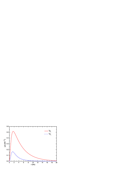
Figure 1: The deuteron ${\rm{}^{3}S_{1}}$ and ${\rm{}^{3}D_{1}}$ wavefunction with binding energy $\varepsilon_{d}\simeq 2.25$ MeV and $\Lambda\simeq 808$ MeV.

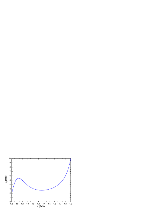
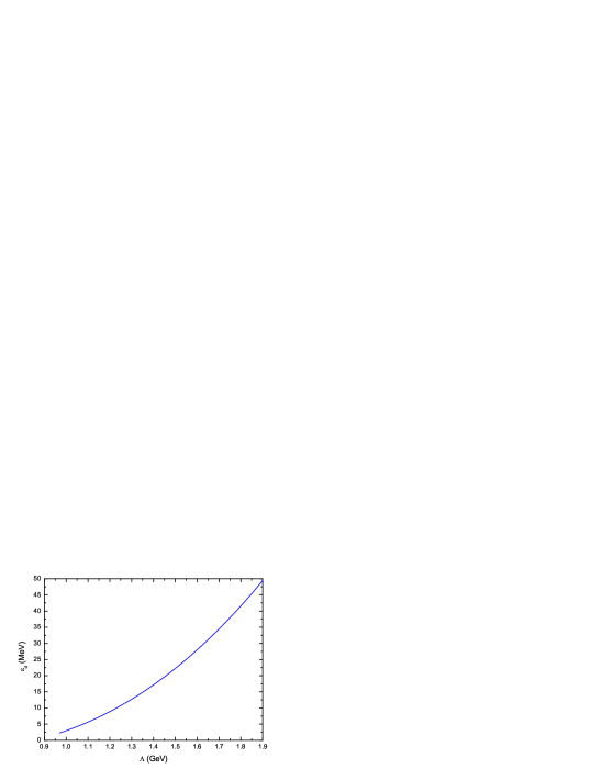
(a)	(b)

Figure 2: The deuteron binding energy variation with respect to the regularization parameter $\Lambda$. Fig. 2a corresponds to the coupling constants shown in Table 1, and Fig. 2b for the couplings reduced by half.

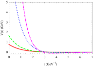
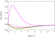
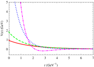
(a)	(b)	(c)

Figure 3: The three components of the deuteron effective potential in Eq.(13), Fig. 3 a, Fig. 3 b and Fig. 3 c respectively illustrate the $V_{11}(\Lambda,r)$, $V_{12}(\Lambda,r)$ and $V_{22}(\Lambda,r)$ components. The solid line, dashed, dotted and dash-dotted lines correspond to $\Lambda=0.8$ GeV, 0.9 GeV, 1.2 GeV and 1.6 GeV respectively.

V Possible ${D\bar{D}^{*}/\bar{D}D^{*}}$ hadronic molecule and X(3872)

The narrow charmoniumlike state X(3872) was discovered by the Belle collaboration in the decay $B^{+}\rightarrow K^{+}+X(3872)$ followed by $X(3872)\rightarrow J/\psi\pi^{+}\pi^{-}$ with a statistical significance of 10.3$\sigma$ Choi:2003ue . The existence of X(3872) has been confirmed by CDF Acosta:2003zx , D0 Abazov:2004kp and Babar collaboration Aubert:2004ns . the CDF collaboration measured the X(3872) mass to be ${\rm(3871.61\pm 0.16(stat)\pm 0.19(sys.))}$ MeV. Its quantum number is strongly preferred to be $1^{++}$ Abulencia:2006ma . In the one pion exchange model, Tornqvist suggested that X(3872) is a $1^{++}$ $D\bar{D}^{*}/\bar{D}D^{*}$ molecule and isospin is strongly broken Tornqvist:2004qy . Recently Close et al. re-analyzed X(3872) in the same model, the critical overall sign is corrected and the contribution of the ”$\delta$ function” term is included Thomas:2008ja . Swanson have taken into account both the long rang pion exchange and short range contribution arising from constituent quark interchange swanson . Recently Zhu et al. dynamically studied the binding of X(3872) in the heavy quark effective theory Liu:2008fh . In this section, we will investigate the $1^{++}$ $D\bar{D}^{*}/\bar{D}D^{*}$ system from the one boson exchange model at quark level, where the short range interactions are represented by the heavier bosons $\eta$, $\sigma$, $\rho$ and $\omega$ exchange instead of the quark interchange.

There is only a sign difference $(-1)^{G}$ between the quark-quark interaction and quark-antiquark interaction, and the magnitudes are the same, where $G$ is the $G$-parity of the exchanged meson. The diagrams contributing to the $D\bar{D}^{*}$ and $\bar{D}D^{*}$ interactions are displayed in Fig. 4. Because of the parity conservation, $D\bar{D}^{*}$ can only scatter into $D^{*}\bar{D}$ via the pseudoscalar $\pi$ and $\eta$ exchange, and $D\bar{D}^{*}$ scatters into $D\bar{D}^{*}$ with the scalar $\sigma$ exchange, whereas the vector mesons $\rho$ and $\omega$ exchange contribute to both processes. The effective potential for the $1^{++}$ $D\bar{D}^{*}/\bar{D}D^{*}$ system is

$$V^{X}(\mathbf{r}) = -V^{X}_{\pi}(\mathbf{r})+V^{X}_{\eta}(\mathbf{r})+V^{X}_{\sigma}(\mathbf{r})+V^{X}_{\rho}(\mathbf{r})-V^{X}_{\omega}(\mathbf{r})$$ (23)

$$\equiv V^{X}_{C}(r)+V^{X}_{S}(r)(\bm{\sigma}_{i}\cdot\bm{\sigma}_{j})+V^{X}_{I}(r)(\bm{\tau}_{i}\cdot\bm{\tau}_{j})+V^{X}_{T}(r)S_{ij}(\mathbf{\hat{r}})+V^{X}_{SI}(\mu_{k},r)(\bm{\sigma}_{i}\cdot\bm{\sigma}_{j})(\bm{\tau}_{i}\cdot\bm{\tau}_{j})$$

$$+V^{X}_{TI}(\mu_{k},r)S_{ij}(\mathbf{\hat{r}})(\bm{\tau}_{i}\cdot\bm{\tau}_{j})+V^{X}_{LS}(r)(\mathbf{L}\cdot\mathbf{S}_{ij})+V^{X}_{LSI}(r)(\mathbf{L}\cdot\mathbf{S}_{ij})(\bm{\tau}_{i}\cdot\bm{\tau}_{j})$$

with $i$ and $j$ is the index of light quark or antiquark, $\mu_{k}(k=1,2,3,4)$ takes four different values due to the mass difference within the $D$, $D^{*}$ and $\pi$ isospin multiplets. The eight components $V^{X}_{C}(r)$, $V^{X}_{S}(r)$ etc are given by

$$V^{X}_{C}({r}) = -\frac{g^{2}_{\sigma qq}}{4\pi}m_{\sigma}\Big{[}H_{0}(\Lambda,m_{\sigma},m_{\sigma},r)+\frac{m^{2}_{\sigma}}{8m^{2}_{q}}H_{1}(\Lambda,m_{\sigma},m_{\sigma},r)\Big{]}-\frac{g^{2}_{\omega qq}}{4\pi}m_{\omega}H_{0}(\Lambda,m_{\omega},m_{\omega},r)$$

$$+\frac{g^{2}_{\omega qq}+4g_{\omega qq}f_{\omega qq}}{4\pi}\frac{m^{3}_{\omega}}{8m^{2}_{q}}H_{1}(\Lambda,m_{\omega},m_{\omega},r)$$

$$V^{X}_{S}({r}) = -\frac{g^{2}_{\eta qq}}{4\pi}\frac{\mu^{3}_{5}}{12m^{2}_{q}}H_{1}(\Lambda,m_{\eta},\mu_{5},r)+\frac{(g_{\omega qq}+f_{\omega qq})^{2}}{4\pi}\frac{\mu^{3}_{7}}{6m^{2}_{q}}H_{1}(\Lambda,m_{\omega},\mu_{7},r)$$

$$V^{X}_{I}({r}) = \frac{g^{2}_{\rho qq}}{4\pi}m_{\rho}H_{0}(\Lambda,m_{\rho},m_{\rho},r)-\frac{g^{2}_{\rho qq}+4g_{\rho qq}f_{\rho qq}}{4\pi}\frac{m^{3}_{\rho}}{8m^{2}_{q}}H_{1}(\Lambda,m_{\rho},m_{\rho},r)$$

$$V^{X}_{T}({r}) = \frac{g^{2}_{\eta qq}}{4\pi}\frac{\mu^{3}_{5}}{12m^{2}_{q}}H_{3}(\Lambda,m_{\eta},\mu_{5},r)+\frac{(g_{\omega qq}+f_{\omega qq})^{2}}{4\pi}\frac{\mu^{3}_{7}}{12m^{2}_{q}}H_{3}(\Lambda,m_{\omega},\mu_{7},r)$$

$$V^{X}_{SI}(\mu,{r}) = \left\{\begin{array}[]{cc}\frac{g^{2}_{\pi qq}}{4\pi}\frac{\mu^{3}}{12m^{2}_{q}}H_{1}(\Lambda,m_{\pi^{\pm,0}},\mu,r)-\frac{(g_{\rho qq}+f_{\rho qq})^{2}}{4\pi}\frac{\mu^{3}_{6}}{6m^{2}_{q}}H_{1}(\Lambda,m_{\rho},\mu_{6},r),&\mu^{2}>0\\ \frac{g^{2}_{\pi qq}}{4\pi}\frac{\tilde{\mu}^{3}}{12m^{2}_{q}}G_{1}(\Lambda,m_{\pi^{\pm,0}},\tilde{\mu},r)-\frac{(g_{\rho qq}+f_{\rho qq})^{2}}{4\pi}\frac{\mu^{3}_{6}}{6m^{2}_{q}}H_{1}(\Lambda,m_{\rho},\mu_{6},r),&~{}~{}~{}~{}~{}~{}\mu^{2}=-\tilde{\mu}^{2}<0\end{array}\right.$$ (26)

$$V^{X}_{TI}(\mu,r) = \left\{\begin{array}[]{cc}-\frac{g^{2}_{\pi qq}}{4\pi}\frac{\mu^{3}}{12m^{2}_{q}}H_{3}(\Lambda,m_{\pi^{\pm,0}},\mu,r)-\frac{(g_{\rho qq}+f_{\rho qq})^{2}}{4\pi}\frac{\mu^{3}_{6}}{12m^{2}_{q}}H_{3}(\Lambda,m_{\rho},\mu_{6},r),&\mu^{2}>0\\ -\frac{g^{2}_{\pi qq}}{4\pi}\frac{\tilde{\mu}^{3}}{12m^{2}_{q}}G_{3}(\Lambda,m_{\pi^{\pm,0}},\tilde{\mu},r)-\frac{(g_{\rho qq}+f_{\rho qq})^{2}}{4\pi}\frac{\mu^{3}_{6}}{12m^{2}_{q}}H_{3}(\Lambda,m_{\rho},\mu_{6},r),&~{}~{}~{}~{}~{}~{}\mu^{2}=-\tilde{\mu}^{2}<0\end{array}\right.$$ (29)

$$V^{X}_{LS}(r) = -\frac{g^{2}_{\sigma qq}}{4\pi}\frac{m^{3}_{\sigma}}{2m^{2}_{q}}H_{2}(\Lambda,m_{\sigma},m_{\sigma},r)+\frac{3g^{2}_{\omega qq}+4g_{\omega qq}f_{\omega qq}}{4\pi}\frac{m^{3}_{\omega}}{2m^{2}_{q}}H_{2}(\Lambda,m_{\omega},m_{\omega},r)$$

$$V^{X}_{LSI}(r) = -\frac{3g^{2}_{\rho qq}+4g_{\rho qq}f_{\rho qq}}{4\pi}\frac{m^{3}_{\rho}}{2m^{2}_{q}}H_{2}(\Lambda,m_{\rho},m_{\rho},r)$$ (30)

where

$$\mu^{2}_{1} = m^{2}_{\pi^{0}}-(m_{D^{*0}}-m_{D^{0}})^{2},~{}~{}~{}~{}~{}\mu^{2}_{2}=m^{2}_{\pi^{\pm}}-(m_{D^{*0}}-m_{D^{\pm}})^{2}$$

$$\mu^{2}_{3} = m^{2}_{\pi^{\pm}}-(m_{D^{*\pm}}-m_{D^{0}})^{2},~{}~{}~{}~{}~{}\mu^{2}_{4}=m^{2}_{\pi^{0}}-(m_{D^{*\pm}}-m_{D^{\pm}})^{2}$$

$$\mu^{2}_{5} = m^{2}_{\eta}-(m_{D^{*0}}-m_{D^{0}})^{2},~{}~{}~{}~{}~{}~{}~{}\mu^{2}_{6}=m^{2}_{\rho}-(m_{D^{*0}}-m_{D^{0}})^{2}$$

$$\mu^{2}_{5} = m^{2}_{\omega}-(m_{D^{*0}}-m_{D^{0}})^{2}$$ (31)

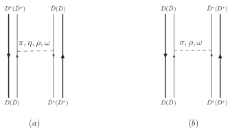
Figure 4: $D\bar{D}^{*}$ and $\bar{D}D^{*}$ interaction in one boson exchange model at quark level, where the thick line represents heavy quark or antiquark, and the thin line denotes light quark or antiquark.

These $\mu^{2}$ parameters approximately represent the recoil effect due to different values of $m_{D}$ and $m_{D^{*}}$ as in Refs. Tornqvist:1993ng ; Thomas:2008ja . For the $\eta$, $\sigma$, $\rho$ and $\omega$ exchange processes, the mass difference of $m_{D^{0}}$ and $m_{D^{\pm}}$ as well as $m_{D^{*0}}$ and $m_{D^{*\pm}}$ are neglected, since they are much smaller comparing with $m_{\eta}$, $m_{\rho}$ and $m_{\omega}$. X(3872) is very close to the $D^{0}\bar{D}^{*0}$ threshold, however, it is about 8.3 MeV below the $D^{+}D^{*-}$ threshold. Hence, isospin symmetry is drastically broken Close:2003sg ; Tornqvist:2004qy . For the $J^{PC}=1^{++}$ $D\bar{D}^{*}/\bar{D}D^{*}$ system, they can be in S wave or D wave similar to the deuteron, then the wavefunction of this system is written as

$$|X(3872)\rangle = \frac{u_{1}(r)}{r}\frac{1}{\sqrt{2}}|(D^{0}\bar{D}^{*0}+\bar{D}^{0}D^{*0})_{S}\rangle+\frac{u_{2}(r)}{r}\frac{1}{\sqrt{2}}|(D^{0}\bar{D}^{*0}+\bar{D}^{0}D^{*0})_{D}\rangle$$ (32)

$$+\frac{u_{3}(r)}{r}\frac{1}{\sqrt{2}}|(D^{+}D^{*-}+D^{-}D^{*+})_{S}\rangle+\frac{u_{4}(r)}{r}\frac{1}{\sqrt{2}}|(D^{+}D^{*-}+D^{-}D^{*+})_{D}\rangle$$

where the subscript $S$ and $D$ denote the system in $S$ wave and $D$ wave respectively. $u_{1}(r)$, $u_{2}(r)$, $u_{3}(r)$ and $u_{4}(r)$ are the spatial wavefunctions. There are four channels coupled with each other as has been shown above, and we might as well choose the basis to be $|1\rangle\equiv\frac{1}{\sqrt{2}}|(D^{0}\bar{D}^{*0}+\bar{D}^{0}D^{*0})_{S}\rangle$, $|2\rangle\equiv\frac{1}{\sqrt{2}}|(D^{0}\bar{D}^{*0}+\bar{D}^{0}D^{*0})_{D}\rangle$, $|3\rangle\equiv\frac{1}{\sqrt{2}}|(D^{+}D^{*-}+D^{-}D^{*+})_{S}\rangle$ and $|4\rangle\equiv\frac{1}{\sqrt{2}}|(D^{+}D^{*-}+D^{-}D^{*+})_{D}\rangle$. Using the analytical formula for the matrix elements presented in the appendix, the effective potential for $1^{++}$ $D\bar{D}^{*}/\bar{D}D^{*}$ can be written in the matrix form as

$$V^{X}(r) = \big{[}V^{X}_{C}(r)+V^{X}_{S}(r)\big{]}\left(\begin{array}[]{cccc}1&0&0&0\\ 0&1&0&0\\ 0&0&1&0\\ 0&0&0&1\end{array}\right)+\big{[}V^{X}_{I}(r)+V^{X}_{SI}(\mu_{k},r)\big{]}\left(\begin{array}[]{cccc}-1&0&-2&0\\ 0&-1&0&-2\\ -2&0&-1&0\\ 0&-2&0&-1\end{array}\right)$$ (59)

$$+V^{X}_{T}(r)\left(\begin{array}[]{cccc}0&-\sqrt{2}&0&0\\ -\sqrt{2}&1&0&0\\ 0&0&0&-\sqrt{2}\\ 0&0&-\sqrt{2}&1\end{array}\right)+V^{X}_{TI}(\mu_{k},r)\left(\begin{array}[]{cccc}0&\sqrt{2}&0&2\sqrt{2}\\ \sqrt{2}&-1&2\sqrt{2}&-2\\ 0&2\sqrt{2}&0&\sqrt{2}\\ 2\sqrt{2}&-2&\sqrt{2}&-1\end{array}\right)$$

$$+V^{X}_{LS}(r)\left(\begin{array}[]{cccc}0&0&0&0\\ 0&-3/2&0&0\\ 0&0&0&0\\ 0&0&0&-3/2\end{array}\right)+V^{X}_{LSI}(r)\left(\begin{array}[]{cccc}0&0&0&0\\ 0&3/2&0&3\\ 0&0&0&0\\ 0&3&0&3/2\end{array}\right)$$

In the above equation, the value of $\mu^{2}_{k}$ is $\mu^{2}_{1}$ for the up-left $2\times 2$ matrix elements, and it is equal to $\mu^{2}_{4}$ for the down-right $2\times 2$ matrix elements. There is ambiguity in choosing $\mu^{2}_{k}$ value for the processes $D^{0}\bar{D}^{*0}\rightarrow D^{*+}D^{-}$ or $D^{+}D^{*-}\rightarrow D^{*0}\bar{D}^{0}$, accordingly $\mu^{2}_{k}$ can take the value $\mu^{2}_{2}$ or $\mu^{2}_{3}$ for the off-diagonal $2\times 2$ matrix elements, the numerical results for both choices would be given in the following. The different $\mu_{k}$ values is due to the isospin symmetry breaking from the mass difference within the $D$, $D^{*}$ and $\pi$ isospin multiplets. Taking into account the centrifugal barrier from D wave and solving the four channel coupled Schr$\ddot{\rm o}$dinger equation using the package FESSDE2.2, the numerical results are listed in Table 3. It is remarkable that the $1^{++}$ $D\bar{D}^{*}/\bar{D}D^{*}$ system could accomodate a molecular state with mass about 3871.6 MeV for $\Lambda=808$ MeV, it is very close to the central value of X(3872) mass 3871.61 MeV. The corresponding wavefunction is shown in Fig. 5, it is obvious that the $D^{0}\bar{D}^{*0}+\bar{D}^{0}D^{*0}$ component dominates over the $D^{+}D^{*-}+D^{-}D^{*+}$ component. Since the spatial wavefunctions $u_{1}(r)$ and $u_{3}(r)$ have the same sign, the same is true for $u_{2}(r)$ and $u_{4}(r)$, thus the $I=0$ component in this state is predominant, it would be a isospin singlet in the isospin symmetry limit. From the results in Table 3, we notice that the predictions about the static properties for the two $\mu^{2}$ choices are very similar to each other, and the difference is small. The isospin symmetry is strongly broken especially for the states near the threshold. The uncertainties induced by the effective coupling constants are considered, we reduce half of the couplings except $g_{\pi NN}$, and the numerical results are given in Table 3 as well. For both choices of the coupling constants, the binding energy and other static properties are sensitive to the regularization parameter $\Lambda$, and the bound state mass dependence on $\Lambda$ is displayed in Fig. 6. It is obvious that the bound state mass decreases monotonically with the regularization parameter $\Lambda$ as in the one pion exchange model. In short summary, the predictions are qualitatively the same as those in the one pion exchange model, even after we have included the contributions from $\eta$, $\sigma$, $\rho$ and $\omega$ exchange. Since unexpectedly large branch ratio of $X(3872)\rightarrow\psi(2S)\gamma$ recently was reported Fulsom:2008rn , we have to take into account the mixing between the $1^{++}$ $D\bar{D}^{*}/\bar{D}D^{*}$ molecule and the conventional charmonium state in order to identify this state with X(3872). This is outside the range of the present work.

$\mu^{2}$	$\Lambda({\rm MeV})$	$~{}~{}~{}{\rm M}(\rm MeV)$	$~{}~{}~{}{\rm r}_{\rm rms}({\rm fm})$	$~{}~{}~{}{\rm P^{00}_{S}:P^{00}_{D}:P^{+-}_{S}:P^{+-}_{D}}(\%)$
	808	3871.6	7.02	90.76:0.56:8.11:0.56
	840	3870.4	2.84	78.23:1.08:19.59:1.11
$\mu^{2}_{3}$	850	3869.8	2.45	75.26:1.21:22.29:1.23
	900	3865.9	1.61	65.17:1.89:31.06:1.88
	1000	3849.2	1.08	53.06:4.72:37.65:4.57
	808	3871.7	11.34	94.40:0.38:4.86:0.36
	840	3870.7	3.19	80.74:0.99:17.26:1.01
$\mu^{2}_{2}$	850	3870.2	2.68	77.44:1.14:20.28:1.15
	900	3866.4	1.66	66.23:1.85:30.09:1.83
	1000	3849.9	1.09	53.35:4.69:37.43:4.53
all couplings except $g_{\pi NN}$ are reduced by half
$\mu^{2}$	$\Lambda({\rm MeV})$	$~{}~{}~{}{\rm M}(\rm MeV)$	$~{}~{}~{}{\rm r}_{\rm rms}({\rm fm})$	$~{}~{}~{}{\rm P^{00}_{S}:P^{00}_{D}:P^{+-}_{S}:P^{+-}_{D}}(\%)$
	970	3869.1	2.13	70.65:1.65:26.02:1.69
$\mu^{2}_{3}$	1100	3860.1	1.25	57.24:2.98:36.83:2.95
	1200	3848.2	1.00	51.80:4.40:39.46:4.33
	970	3869.5	2.28	72.56:1.57:24.28:1.60
$\mu^{2}_{2}$	1100	3860.8	1.27	57.76:2.94:36.38:2.92
	1200	3849.0	1.01	52.04:4.38:39.29:4.30

Table 3: The predictions about the mass, the root of mean square radius(rms) and the probabilities of the different components for the $1^{++}$ $D\bar{D}^{*}/\bar{D}D^{*}$ molecule.

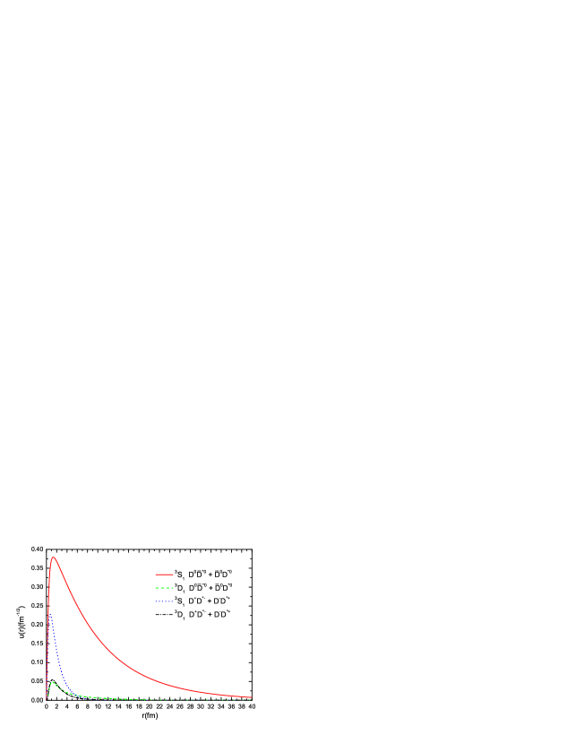
Figure 5: The four components spatial wavefunctions of the $1^{++}$ $D\bar{D}^{*}/\bar{D}D^{*}$ system with $\Lambda=808$ MeV.

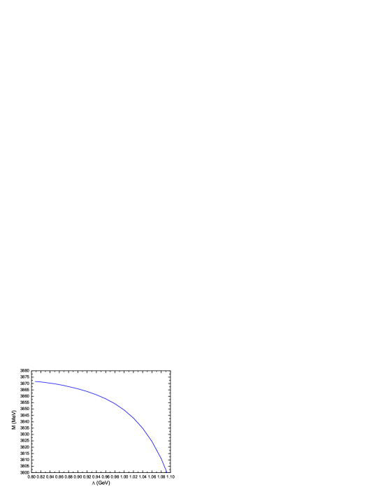
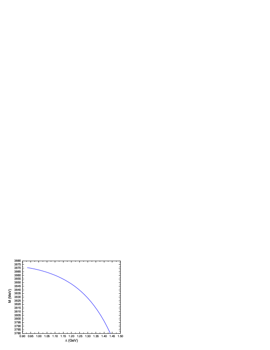
(a)	(b)

Figure 6: The variation of the $1^{++}$ $D\bar{D}^{*}/\bar{D}D^{*}$ bound state mass with respect to $\Lambda$. (a) corresponds to the coupling constants shown in Table 1, and (b) for the couplings reduced by half.

VI Possible molecular states of other heavy flavor PV systems

VI.1 $B\bar{B}^{*}/\bar{B}B^{*}$ system

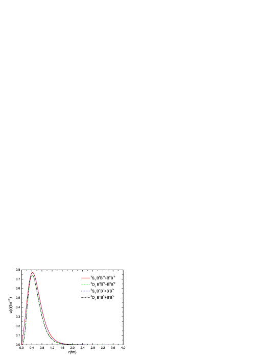
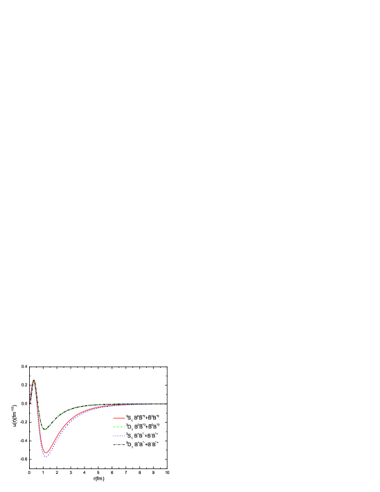
(a)	(b)

Figure 7: The spatial wavefunctions of $1^{++}$ $B\bar{B}^{*}/\bar{B}B^{*}$ molecule with $\Lambda=1000$ MeV. There are two bound states with mass 10457.6 MeV and 10600.4 MeV respectively, Fig. 7a is for the first state, and the Fig. 7b for the second.

For the $1^{++}$ $B\bar{B}^{*}/\bar{B}B^{*}$ system, the kinetic energy is greatly reduced due to the heavier mass of $B$ meson, and the interaction potential has features similar to those of the $D\bar{D}^{*}/\bar{D}D^{*}$ system except that the former is deeper than the latter. Therefore molecular states should be more easily formed. Following the same procedure as the $D\bar{D}^{*}/\bar{D}D^{*}$ case, the numerical results are shown in Table 4, where the $\mu^{2}$ ambiguity is considered. For the same value of $\Lambda$, the $B\bar{B}^{*}/\bar{B}B^{*}$ system is really more strongly bound than the $D\bar{D}^{*}/\bar{D}D^{*}$ system, its binding energy is a few tens of MeV, and the same was predicted in the one pion exchange model Tornqvist:1993ng ; Thomas:2008ja and in the models Liu:2008fh ; liu-chiral . It is obvious that the predictions about the static properties for the two $\mu^{2}$ choices are approximately the same. We notice that the isospin symmetry breaking is less stronger than the charm system, this is because the mass difference of $B^{0}$ and $B^{+}$ is smaller than that of $D^{0}$ and $D^{+}$ as well as $D^{*0}$ and $D^{*+}$. It is notable that there may be two molecular states for appropriate values of $\Lambda$. The corresponding wavefunctions for $\Lambda=1000$ MeV and $\mu^{2}=\mu^{2}_{bb1}\equiv m^{2}_{\pi^{\pm}}-(m_{B^{*}}-m_{B^{0}})^{2}$ are displayed in Fig. 7, the first state is tightly bound, whereas the second is loosely bound. We notice that the first state is almost an isospin singlet, and the $I=0$ component is dominant for the second state. This state can no longer be produced through $B$ meson decay because of its large mass, and we have to resort to hadron collider. We can search for this state at Tevatron via $p\bar{p}\rightarrow\pi^{+}\pi^{-}\Upsilon(1S)$, and LHC is more promising.

VI.2 $DD^{*}$ system with $C=2$

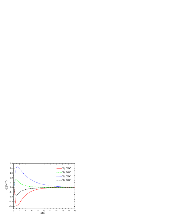
Figure 8: The wavefunction for the $DD^{*}$ system assuming $\Lambda=1600$ MeV and $\mu^{2}=\mu^{2}_{cc1}\equiv m^{2}_{\pi^{0}}-(m_{D^{*+}}-m_{D^{+}})^{2}$, its mass approximately is 3873.9 MeV.

The interaction potentials arise from the one boson exchange between two antiquarks instead of a quark and antiquark pair, hence both the $\pi$ exchange and $\omega$ exchange potentials have overall opposite sign relative to the $D\bar{D}^{*}/\bar{D}D^{*}$ case. In this case we have four coupled channels $(D^{+}D^{*0})_{S}$, $(D^{+}D^{*0})_{D}$, $(D^{0}D^{*+})_{S}$ and $(D^{0}D^{*+})_{D}$. The numerical results are given in Table 5. For $\Lambda=808$ MeV or $\Lambda=970$ MeV, we find no bound state. A bound state with mass about 3873.9 MeV appears for $\Lambda=1600$ MeV (about 3873.1 MeV for $\Lambda=1900$ MeV if the couplings except $g_{\pi NN}$ are reduced half), and the corresponding wavefunction is shown in Fig. 8. We notice that the wavefunctions of ${}^{3}S_{1}$ $D^{+}D^{*0}$ and $D^{0}D^{*+}$ have opposite signs, the same is true for the ${}^{3}D_{1}$ $D^{+}D^{*0}$ and $D^{0}D^{*+}$ wavefunctions, therefore this state would be a isospin singlet in the isospin symmetry limit. We notice that the ${}^{3}D_{1}$ probability are much larger than ${}^{3}S_{1}$ probability for the state with $\Lambda=1800$ MeV, although there is centrifugal barrier for the D wave state. Thus the S-D mixing effect induced by the tensor force is especially crucial for this state. In short, the bound state of the $DD^{*}$ system appears only for the regularization parameter $\Lambda$ as large as 1600 MeV or 1900 MeV, which is beyond the range of 0.8 to 1.5 GeV favored by the nucleon-nucleon interaction. Moreover, the parameters that allow X(3872) to emerge as a $D\bar{D}^{*}/\bar{D}D^{*}$ molecule exclude the $DD^{*}$ bound state, as can be seen from the results in section V. Consequently we tend to conclude that the $DD^{*}$ molecular state may not exist.

VI.3 $BB^{*}$ system with $B=2$

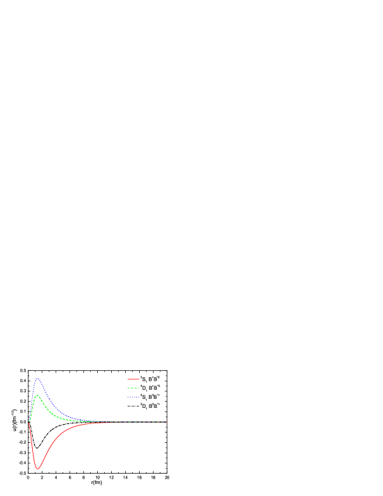
Figure 9: The spatial wavefunction for the $BB^{*}$ system assuming $\Lambda=900$ MeV and $\mu^{2}=\mu^{2}_{bb1}\equiv m^{2}_{\pi^{0}}-(m_{B^{*}}-m_{B^{+}})^{2}$, its mass is 10602.3 MeV.

The situation is very similar to the $DD^{*}$ system except the different mass of $D$ mesons and $B$ mesons, we list the numerical results in Table 6. We find a marginally bound state with mass 10603.9 MeV for $\Lambda=808$ MeV, which is very close to the $BB^{*}$ threshold. Its binding energy is much smaller than that of the $1^{++}$ $B\bar{B}^{*}/\bar{B}B^{*}$ system, however, the binding energy is less sensitive to $\Lambda$ than the latter case. Fig. 9 displays the wavefunction of the bound state solution with mass 10602.3 MeV and $\Lambda=900$ MeV. It is obvious that the $B^{+}B^{*0}$ and $B^{0}B^{*+}$ wavefunctions have the opposite sign, then the $I=0$ component is dominant in this state. If the couplings except $g_{\pi NN}$ are reduced by half, a weakly bound state with mass about 10601.5 MeV is found as well assuming $\Lambda=970$ MeV. These indicates a weakly bound $BB^{*}$ should exist, This is consistent with the results of Manohar and Wise form heavy quark effective theory manohar . For a loosely bound molecule, the leading source of decay is dissociation, to a good approximation the dissociation will proceed via the free space decay of the constituent mesons. The spin-parity forbids its decay into $BB$, therefore the $BB^{*}$ molecule is a very narrow state and it mainly decays into $BB\gamma$.

VI.4 Pseudoscalar-vector system with $C=B=1$

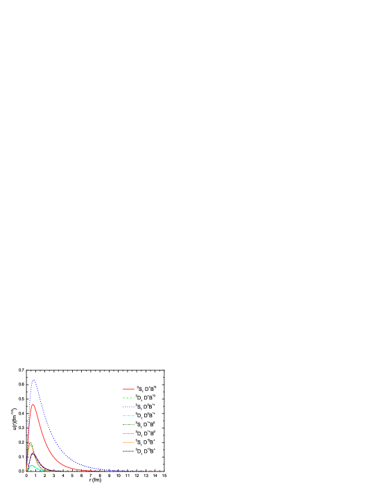
Figure 10: The wavefunction of the $C=B=1$ pseudoscalar-vector system with $\Lambda=900$ MeV and $\mu^{2}=m^{2}_{ex}-(m_{D^{*}}-m_{D})^{2}$, the mass of this state is about 7185.9 MeV.

This system could have the same quantum as $B_{c}$ meson or its antiparticle, and it is different from all the systems discussed above, eight channels instead of four channels are coupled with each other under the one boson exchange interaction, i.e. $(D^{+}B^{*0})_{S}$, $(D^{+}B^{*0})_{D}$, $(D^{0}B^{*+})_{S}$, $(D^{0}B^{*+})_{D}$, $(D^{*+}B^{0})_{S}$, $(D^{*+}B^{0})_{D}$, $(D^{*0}B^{+})_{S}$ and $(D^{*0}B^{+})_{D}$. We can investigate the possible bound states along the same line, although it is somewhat lengthy and tedious. There is ambiguity in choosing the $\mu^{2}$ value as well, for the $DB^{*}\rightarrow D^{*}B$ scattering process, we could take $\mu^{2}=m^{2}_{ex}-(m_{D^{*}}-m_{D})^{2}$ or $\mu^{2}=m^{2}_{ex}-(m_{B^{*}}-m_{B})^{2}$, where $m_{ex}$ is the mass of the exchanged boson. Specifically for $D^{+}B^{*0}\rightarrow D^{*+}B^{0}$ via $\pi$ exchange, we can choose $\mu^{2}=m^{2}_{\pi^{0}}-(m_{D^{*+}}-m_{D^{+}})^{2}$ or $\mu^{2}=m^{2}_{\pi^{0}}-(m_{B^{*0}}-m_{B^{0}})^{2}$. This ambiguity has been taken into account in our analysis. The numerical results are given in Table 7, For $\Lambda=808$ MeV, we find no bound state. With the choice $\mu^{2}=m^{2}_{ex}-(m_{D^{*}}-m_{D})^{2}$, a bound state with mass 7189.7 MeV is found for $\Lambda=850$ MeV, However, this solution disappears if one chooses $\mu^{2}=m^{2}_{ex}-(m_{B^{*}}-m_{B})^{2}$. Only when $\Lambda$ is around 880 MeV, the bound state solutions can be found for both $\mu^{2}$ choices. The difference of the static properties for the two $\mu^{2}$ choices is relatively larger than that of the above systems considered, this is because of the larger difference between $m_{D^{*}}-m_{D}\simeq 140$ MeV and $m_{B^{*}}-m_{B}\simeq 45$ MeV. We notice that the $D^{0}B^{*+}$ component has the largest probability in the states, since the threshold of $D^{0}B^{*+}$ is lower than that of $D^{+}B^{*0}$, $D^{*+}B^{0}$ and $D^{*0}B^{+}$. The wavefunction of the state with mass about 7185.9 MeV and $\Lambda=900$ MeV is shown in Fig. 10, it is obvious all the eight components of the spatial wavefunction have the same sign, consequently this state would be isospin singlet in the isospin symmetry limit. Similar pattern of bound state solutions is predicted if the coupling constants except $g_{\pi NN}$ are reduced by half. This state is difficult to be produced, since both $c$ and $\bar{b}$ have to be produced simultaneously. The direct production of this state at hadron collider such as LHC and Tevatron is most promising, and the indirect production via top quark decay is a possible alternative. Once produced, it should be very stable, $DB\pi$ and $DB\gamma$ are the main decay channels.

VI.5 Pseudoscalar-vector system with $C=-B=1$

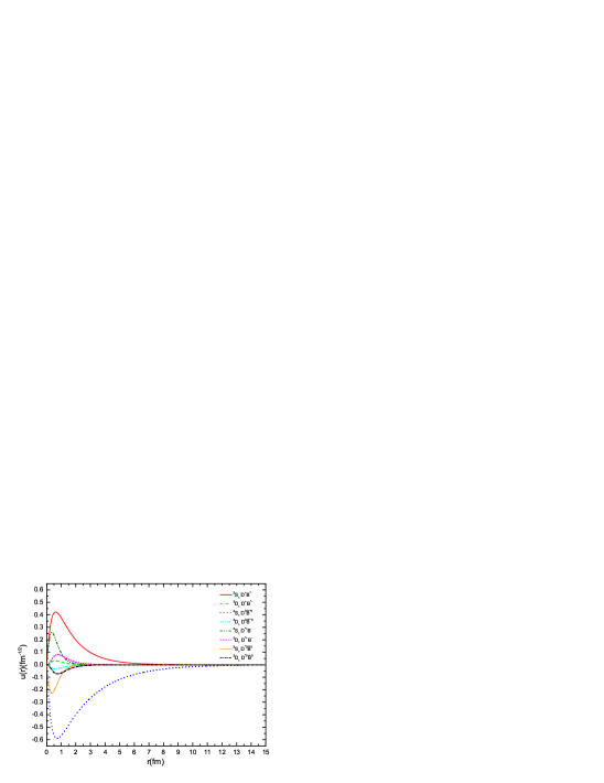
Figure 11: The wavefunction of the $C=-B=1$ pseudoscalar-vector system with $\Lambda=900$ MeV and $\mu^{2}=m^{2}_{ex}-(m_{D^{*}}-m_{D})^{2}$, its mass is about 7187.6 MeV.

The effective interaction potentials are induced by one boson exchange between two antiquarks, therefore both the $\pi$ exchange and $\omega$ exchange contributions give opposite sign between the $C=B=1$ system and the $C=-B=1$ system, nevertheless the overall signs of $\eta$, $\sigma$ and $\rho$ exchange potentials remain. We have eight coupled channels as well, $(D^{+}B^{*-})_{S}$, $(D^{+}B^{*-})_{D}$, $(D^{0}\bar{B}^{*0})_{S}$, $(D^{0}\bar{B}^{*0})_{D}$, $(D^{*+}B^{-})_{S}$, $(D^{*+}B^{-})_{D}$, $(D^{*0}\bar{B}^{0})_{S}$ and $(D^{*0}\bar{B}^{0})_{D}$ are involved. The numerical results are given in Table 8. It is remarkable that the $\mu^{2}$ and $\Lambda$ dependence of the bound state solutions is similar to the $C=B=1$ case. With the same $\mu^{2}$ and $\Lambda$ values, the predictions for the static properties of the two systems are not drastically different from each other. Concretely for $\Lambda=900$ MeV and $\mu^{2}=m^{2}_{ex}-(m_{D^{*}}-m_{D})^{2}$, we find a bound state with mass 7187.6 MeV for the $C=-B=1$ system, and the mass of $C=B=1$ bound state is 7185.9 MeV, the difference is about 1.7 MeV. The corresponding wavefunction with $\Lambda=900$ MeV is plotted in Fig. 11, which can be roughly obtained by reversing the overall sign of the third, fourth, seventh and eighth components of the $C=B=1$ system wavefunction in Fig. 10. To understand the similarity of the predictions for the $C=B=1$ and $C=-B=1$ system, we turn to the one $\pi$ exchange model, the effective potential comprises a spin-spin potential proportional to $(\bm{\sigma}_{i}\cdot\bm{\sigma}_{j})(\bm{\tau}_{i}\cdot\bm{\tau}_{j})$ and a tensor potential proportional to $S_{ij}(\hat{\mathbf{r}})(\bm{\tau}_{i}\cdot\bm{\tau}_{j})$, where the isospin matrix $\bm{\tau}_{i}$ and the spin matrix $\bm{\sigma}_{i}$ only act on the light quarks. In the basis of the eight channels listed above, these two operators can be written as $8\times 8$ matrices

$$(\bm{\sigma}_{i}\cdot\bm{\sigma}_{j})(\bm{\tau}_{i}\cdot\bm{\tau}_{j})\longrightarrow\left(\begin{array}[]{cccccccc}0&0&0&0&-1&0&2&0\\ 0&0&0&0&0&-1&0&2\\ 0&0&0&0&2&0&-1&0\\ 0&0&0&0&0&2&0&-1\\ -1&0&2&0&0&0&0&0\\ 0&-1&0&2&0&0&0&0\\ 2&0&-1&0&0&0&0&0\\ 0&2&0&-1&0&0&0&0\end{array}\right)$$ (68)

$$S_{ij}(\hat{\mathbf{r}})(\bm{\tau}_{i}\cdot\bm{\tau}_{j})\longrightarrow\left(\begin{array}[]{cccccccc}0&0&0&0&0&\sqrt{2}&0&-2\sqrt{2}\\ 0&0&0&0&\sqrt{2}&-1&-2\sqrt{2}&2\\ 0&0&0&0&0&-2\sqrt{2}&0&\sqrt{2}\\ 0&0&0&0&-2\sqrt{2}&2&\sqrt{2}&-1\\ 0&\sqrt{2}&0&-2\sqrt{2}&0&0&0&0\\ \sqrt{2}&-1&-2\sqrt{2}&2&0&0&0&0\\ 0&-2\sqrt{2}&0&\sqrt{2}&0&0&0&0\\ -2\sqrt{2}&2&\sqrt{2}&-1&0&0&0&0\end{array}\right)$$ (77)

For the $C=B=1$ pseudoscalar-vector system, the corresponding matrix representations are obtained by replacing 2 and $2\sqrt{2}$ with -2 and $-2\sqrt{2}$ respectively in Eq.(77). It is obvious both operators contribute to only the off-diagonal $4\times 4$ matrix elements. As a result, the eigenvalues of the corresponding Schr$\ddot{\rm o}$dinger equation for the $C=B=1$ and $C=-B=1$ cases are exactly the same, if the small mass difference within the isospin multiplets is neglected, and the eingen-wavefunction of one system can be obtained from another by reversing the overall sign of the third, fourth, seventh and eighth components. Therefore the heavy bosons $\eta$, $\sigma$, $\rho$ and $\omega$ exchange contributes to effective potential, and the pion exchange contribution is still dominant. In short summary, even after including shorter distance contributions from $\eta$, $\sigma$, $\rho$ and $\omega$ exchange, the results obtained are qualitatively the same as those in the one $\pi$ exchange model. The same conclusion has been reached for all the system consider above.

VII Conclusions and discussions

Motivated by the nucleon-nucleon interaction, we have represented the short range interaction by heavier mesons $\eta$, $\sigma$, $\rho$ and $\omega$ exchange. The effective potentials between two hadrons are obtained by summing the interactions between light quarks or antiquarks via one boson exchange. The potential becomes more complicated than that in the one pion exchange model, and there are six additional terms which are proportional to $\mathbf{1}$, $\bm{\tau}_{i}\cdot\bm{\tau}_{j}$, $\bm{\sigma}_{i}\cdot\bm{\sigma}_{j}$, $S_{ij}(\hat{\mathbf{r}})$, $\mathbf{L}\cdot\mathbf{S}_{ij}$ and $(\mathbf{L}\cdot\mathbf{S}_{ij})(\bm{\tau}_{i}\cdot\bm{\tau}_{j})$ respectively.

We first apply the one boson exchange formalism to the deuteron, then generalize to $D\bar{D}^{*}/\bar{D}D^{*}$, $B\bar{B}^{*}/\bar{B}B^{*}$, $DD^{*}$, $BB^{*}$, PV systems with $C=B=1$ and $C=-B=1$. S-D mixing effects has been taken into account, and the uncertainties from the regularization parameter $\Lambda$ and effective coupling constants are considered. We find the conclusions reached are qualitatively the same as those in the one pion exchange model. This implies that the long range $\pi$ exchange effects dominate the physics of a weakly bound hadronic molecule, and we can safely use one pion exchange model to qualitatively discuss the binding of molecule candidates. Since the predictions for the binding energy and other static properties are sensitive to the regularization parameter $\Lambda$ and the effective couplings, we are not able to predict the binding energies very precisely. If the potential is so strong that binding energy is large enough, we would be quite confident that such bound state must exist. However, the exact binding energy will depend on the details of the regularization and the effective couplings involved. Our results indicate that the $1^{++}$ $B\bar{B}^{*}/\bar{B}B^{*}$ molecule should exist, whereas $DD^{*}$ bound state doesn’t exist. For $\Lambda=808$ MeV (970 MeV), the binding energy, D wave probability and other static properties of deuteron are produced, meanwhile near threshold $1^{++}$ $D\bar{D}^{*}/\bar{D}D^{*}$ molecule is predicted. To identify this state with X(3872), the mixing between this $D\bar{D}^{*}/\bar{D}D^{*}$ molecule and the conventional charmonium state should be further considered to be consistent with the recent experimental data on $X(3872)\rightarrow\psi(2S)\gamma$ Fulsom:2008rn . For the $BB^{*}$ system, the PV systems with $C=B=1$ and $C=-B=1$, near threshold molecular states may exist. Similar to the $1^{++}$ $D\bar{D}^{*}/\bar{D}D^{*}$ molecule, these states should be rather stable, isospin is drastically broken, and the $I=0$ component is dominant. Direct production of the above doubly heavy states at Tevatron and LHC is the most promising way. We can search for the $1^{++}$ $B\bar{B}^{*}/\bar{B}B^{*}$ molecule via $p\bar{p}\rightarrow\pi^{+}\pi^{-}\Upsilon(1S)$ at Tevatron. The $BB^{*}$ bound state mainly decays into $BB\gamma$ if it really exists. The dominant decay channels of the heavy flavor PV bound state with $C=B=1$ are $DB\pi$ and $DB\gamma$, and the possible heavy flavor PV bound state with $C=-B=1$ mainly decays into $D\bar{B}\pi$ and $D\bar{B}\gamma$.

In our model, the involved parameters include the effective quark-boson couplings, the masses of the exchanged bosons and the hadrons inside the molecule. Therefore this model is quite general, it can be widely used to dynamically study the possible molecular candidates. We will further apply the one boson exchange model to baryon-antibaryon system etc, and compare the predictions with the recent experimental observations progress .

Appendix A The matrix elements of the spin relevant operators

For initial state consisting of two mesons $A$ and $B$, with relative angular momentum $L$, total spin $S$ and total angular momentum $J$, its wavefunction is written as

$$|(AB)LS,JM_{J}\rangle=\sum_{M_{L},M_{S}}\langle LM_{L};SM_{S}|JM_{J}\rangle\;|LM_{L}\rangle|SM_{S}\rangle$$

$$=\sum_{S_{13},S_{24}}\hat{S}_{A}\hat{S}_{B}\hat{S}_{13}\hat{S}_{24}\left\{\begin{array}[]{ccc}1/2&1/2&S_{A}\\ 1/2&1/2&S_{B}\\ S_{13}&S_{24}&S\end{array}\right\}|L(S_{13}S_{24})S,JM_{J}\rangle$$ (81)

where $\hat{S}=\sqrt{2S+1}$. For the convenience of calculating the matrix elements of the spin-orbit operator $\mathbf{L}\cdot\mathbf{S}_{24}$, we can recouple the state as

$$|(AB)LS,JM_{J}\rangle= \sum_{S_{13},S_{24},J_{LS}}(-1)^{L+S+J}\hat{S}_{A}\hat{S}_{B}\hat{S}_{13}\hat{S}_{24}\hat{S}\hat{J}_{LS}\left\{\begin{array}[]{ccc}L&S_{24}&J_{LS}\\ S_{13}&J&S\end{array}\right\}\left\{\begin{array}[]{ccc}1/2&1/2&S_{A}\\ 1/2&1/2&S_{B}\\ S_{13}&S_{24}&S\end{array}\right\}$$ (88)

$$\times|(LS_{24})J_{LS}S_{13},JM_{J}\rangle$$

In the same way, we can recouple the the final state $|(A^{\prime}B^{\prime})L^{\prime}S^{\prime},J^{\prime}M^{\prime}_{J}\rangle$ via the Wigner 6-j and 9-j coefficients. In the following, we shall present the matrix elements of four light quark operators involved in the work, which is helpful to calculating the matrix representation of the effective interactions.

1. The unit operator $\mathbf{1}$
   Using Eq.(81), it is obvious that

   $$\langle(A^{\prime}B^{\prime})L^{\prime}S^{\prime},J^{\prime}M^{\prime}_{J}|\mathbf{1}|(AB)LS,JM_{J}\rangle=\delta_{LL^{\prime}}\delta_{SS^{\prime}}\delta_{JJ^{\prime}}\delta_{M_{J}M^{\prime}_{J}}\sum_{S_{13},S_{24}}\hat{S}_{A}\hat{S}^{\prime}_{A}\hat{S}_{B}\hat{S}^{\prime}_{B}\hat{S}^{2}_{13}\hat{S}^{2}_{24}$$

   $$\times\left\{\begin{array}[]{ccc}1/2&1/2&S_{A}\\ 1/2&1/2&S_{B}\\ S_{13}&S_{24}&S\end{array}\right\}\left\{\begin{array}[]{ccc}1/2&1/2&S^{\prime}_{A}\\ 1/2&1/2&S^{\prime}_{B}\\ S_{13}&S_{24}&S\end{array}\right\}=\delta_{LL^{\prime}}\delta_{SS^{\prime}}\delta_{S_{A}S^{\prime}_{A}}\delta_{S_{B}S^{\prime}_{B}}\delta_{JJ^{\prime}}\delta_{M_{J}M^{\prime}_{J}}$$ (95)

2. The spin-spin operator $\bm{\sigma}_{2}\cdot\bm{\sigma}_{4}$

   $$\langle(A^{\prime}B^{\prime})L^{\prime}S^{\prime},J^{\prime}M^{\prime}_{J}|\bm{\sigma}_{2}\cdot\bm{\sigma}_{4}|(AB)LS,JM_{J}\rangle=\delta_{LL^{\prime}}\delta_{SS^{\prime}}\delta_{JJ^{\prime}}\delta_{M_{J}M^{\prime}_{J}}\sum_{S_{13},S_{24}}\hat{S}_{A}\hat{S}^{\prime}_{A}\hat{S}_{B}\hat{S}^{\prime}_{B}\hat{S}^{2}_{13}\hat{S}^{2}_{24}$$

   $$\times[2S_{24}(S_{24}+1)-3]\left\{\begin{array}[]{ccc}1/2&1/2&S_{A}\\ 1/2&1/2&S_{B}\\ S_{13}&S_{24}&S\end{array}\right\}\left\{\begin{array}[]{ccc}1/2&1/2&S^{\prime}_{A}\\ 1/2&1/2&S^{\prime}_{B}\\ S_{13}&S_{24}&S\end{array}\right\}$$ (102)

   where the spin operators $\bm{\sigma}_{2}$ and $\bm{\sigma}_{4}$ only act on the light quarks and antiquarks

3. The spin-orbit operator $\mathbf{L}\cdot\mathbf{S}_{24}$

   $$\langle(A^{\prime}B^{\prime})L^{\prime}S^{\prime},J^{\prime}M^{\prime}_{J}|\mathbf{L}\cdot\mathbf{S}_{24}|(AB)LS,JM_{J}\rangle=\delta_{LL^{\prime}}\delta_{JJ^{\prime}}\delta_{M_{J}M^{\prime}_{J}}\sum_{S_{13},S_{24},J_{LS}}(-1)^{S+S^{\prime}+2L+2J}\hat{S}_{A}\hat{S}^{\prime}_{A}$$

   $$\times\hat{S}_{B}\hat{S}^{\prime}_{B}\hat{S}\hat{S}^{\prime}\hat{S}^{2}_{13}\hat{S}^{2}_{24}\hat{J}^{2}_{LS}\frac{1}{2}[J_{LS}(J_{LS}+1)-L(L+1)-S_{24}(S_{24}+1)]\left\{\begin{array}[]{ccc}L&S_{24}&J_{LS}\\ S_{13}&J&S\end{array}\right\}$$ (105)

   $$\times\left\{\begin{array}[]{ccc}L&S_{24}&J_{LS}\\ S_{13}&J&S^{\prime}\end{array}\right\}\left\{\begin{array}[]{ccc}1/2&1/2&S_{A}\\ 1/2&1/2&S_{B}\\ S_{13}&S_{24}&S\end{array}\right\}\left\{\begin{array}[]{ccc}1/2&1/2&S^{\prime}_{A}\\ 1/2&1/2&S^{\prime}_{B}\\ S_{13}&S_{24}&S\end{array}\right\}$$ (114)

   where $\mathbf{S}_{24}=\frac{1}{2}(\bm{\sigma}_{2}+\bm{\sigma}_{4})$, $\mathbf{L}$ is the relative spatial angular momentum. The matrix elements of $\mathbf{L}\cdot\mathbf{S}_{24}$ can be calculated by the Wigner-Echart theorem angular , and the same result has been obtained.

4. The tensor operator $S_{24}(\hat{\mathbf{r}})\equiv 3(\bm{\sigma}_{2}\cdot\hat{\bf r})(\bm{\sigma}_{4}\cdot\hat{\bf r})-\bm{\sigma}_{2}\cdot\bm{\sigma}_{4}$
   It can be checked that the tensor operator $S_{24}(\hat{r})$ is proportional to the scalar product of two rank-2 tensor operators $Y_{2m}$ and $S^{(2)}_{m}$ with $m=0,\pm 1,\pm 2$, where $Y_{2m}$ is the spherical harmonic function of degree 2, and the five components of $S^{(2)}_{m}$ are

   $$S^{(2)}_{2}=\frac{1}{2}S_{2+}S_{4+},~{}~{}~{}S^{(2)}_{1}=-\frac{1}{2}(S_{20}S_{4+}+S_{2+}S_{40}),~{}~{}~{}S^{(2)}_{0}=-\frac{\sqrt{6}}{12}(S_{2-}S_{4+}-4S_{20}S_{40}+S_{2+}S_{4-})$$

   $$S^{(2)}_{-1}=\frac{1}{2}(S_{2-}S_{40}+S_{20}S_{4-}),~{}~{}~{}S^{(2)}_{-2}=\frac{1}{2}S_{2-}S_{4-}$$ (115)

   Here $S_{2+}=\frac{1}{2}(\sigma_{2x}+i\sigma_{2y})$, $S_{20}=\frac{1}{2}\sigma_{20}$ and $S_{2-}=\frac{1}{2}(\sigma_{2x}-i\sigma_{2y})$. The same convention applies to $S_{4,\pm}$ and $S_{40}$, the spin operators $\bm{\sigma}_{2}$ and $\bm{\sigma}_{4}$ only act on the light quark and antiquarks. Using the Wigner-Echart theorem, the matrix element of this tensor operator can be obtained, although it is somewhat lengthy.

   $$\langle(A^{\prime}B^{\prime})L^{\prime}S^{\prime},J^{\prime}M^{\prime}_{J}|S_{24}(\hat{\mathbf{r}})|(AB)LS,JM_{J}\rangle=\delta_{JJ^{\prime}}\delta_{M_{J}M^{\prime}_{J}}\frac{2}{3}\sqrt{30}\sum_{S_{13},S_{24}}\delta_{S_{24},1}(-1)^{J+L+L^{\prime}+2S^{\prime}+S_{13}+S_{24}}$$

   $$\times\hat{S}_{A}\hat{S}^{\prime}_{A}\hat{S}_{B}\hat{S}^{\prime}_{B}\hat{S}\hat{S}^{\prime}\hat{L}\hat{L}^{\prime}\hat{S}^{2}_{13}\hat{S}^{4}_{24}\left\{\begin{array}[]{ccc}L^{\prime}&S^{\prime}&J\\ S&L&2\end{array}\right\}\left\{\begin{array}[]{ccc}S_{24}&S^{\prime}&S_{13}\\ S&S_{24}&2\end{array}\right\}\left(\begin{array}[]{ccc}L^{\prime}&2&L\\ 0&0&0\end{array}\right)\left\{\begin{array}[]{ccc}1/2&1/2&S_{A}\\ 1/2&1/2&S_{B}\\ S_{13}&S_{24}&S\end{array}\right\}$$ (125)

   $$\times\left\{\begin{array}[]{ccc}1/2&1/2&S^{\prime}_{A}\\ 1/2&1/2&S^{\prime}_{B}\\ S_{13}&S_{24}&S^{\prime}\end{array}\right\}$$ (129)

   The above expression is apparently different from the results in Ref. Thomas:2008ja , However, the numerical results of all the matrix elements are the same.

$1^{++}$ $B\bar{B}^{*}/\bar{B}B^{*}$
$\mu^{2}$	$\Lambda({\rm MeV})$	$~{}~{}~{}{\rm M}(\rm MeV)$	$~{}~{}~{}{\rm r}_{\rm rms}({\rm fm})$	$~{}~{}~{}{\rm P^{00}_{S}:P^{00}_{D}:P^{+-}_{S}:P^{+-}_{D}}(\%)$
	808	10565.3	0.60	47.70:2.05:48.20:2.05
$\mu^{2}_{b\bar{b}1}$	900	10543.5	0.59	44.11:5.69:44.50:5.70
	1000	10457.6	0.52	27.52:22.41:27.64:22.44
		10600.4	1.73	37.10:9.43:44.26:9.22
	808	10565.3	0.60	47.70:2.05:48.20:2.05
$\mu^{2}_{b\bar{b}2}$	900	10543.5	0.59	44.11:5.69:44.49:5.70
	1000	10457.6	0.52	27.52:22.41:27.64:22.44
		10600.4	1.72	37.10:9.43:44.25:9.22
all coupling except $g_{\pi NN}$ are reduced by half
$\mu^{2}$	$\Lambda({\rm MeV})$	$~{}~{}~{}{\rm M}(\rm MeV)$	$~{}~{}~{}{\rm r}_{\rm rms}({\rm fm})$	$~{}~{}~{}{\rm P^{00}_{S}:P^{00}_{D}:P^{+-}_{S}:P^{+-}_{D}}(\%)$
	970	10544.8	0.55	45.24:4.60:45.55:4.61
$\mu^{2}_{b\bar{b}1}$	1100	10503.9	0.51	40.12:9.78:40.30:9.80
	1200	10443.1	0.46	33.66:16.27:33.77:16.29
		10601.9	1.91	38.82:8.03:45.26:7.89
	970	10544.8	0.55	45.24:4.60:45.55:4.61
$\mu^{2}_{b\bar{b}2}$	1100	10503.9	0.51	40.12:9.78:40.30:9.80
	1200	10443.1	0.46	33.66:16.27:33.77:16.29
		10601.9	1.91	38.83:8.04:45.25:7.89

Table 4: The predictions about the mass, the root of mean square radius(rms) and the probabilities of the different components for the $1^{++}$ $B\bar{B}^{*}/\bar{B}B^{*}$ system with $\mu^{2}_{b\bar{b}1}=m^{2}_{\pi^{\pm}}-(m_{B^{*}}-m_{B^{0}})^{2}$ and $\mu^{2}_{b\bar{b}2}=m^{2}_{\pi^{\pm}}-(m_{B^{*}}-m_{B^{+}})^{2}$.

${DD^{*}}$ system with $C=2$
$\mu^{2}$	$\Lambda({\rm MeV})$	$~{}~{}~{}{\rm M}(\rm MeV)$	$~{}~{}~{}{\rm r}_{\rm rms}({\rm fm})$	$~{}~{}~{}{\rm P^{+0}_{S}:P^{+0}_{D}:P^{0+}_{S}:P^{0+}_{D}}(\%)$
	1600	3873.9	3.15	34.61:4.03:56.82:4.54
$\mu^{2}_{cc1}$	1700	3865.1	1.30	20.29:28.37:22.63:28.71
	1800	3770.9	0.58	0.19:49.78:0.19:49.84
		3872.8	2.48	41.47:1.38:55.54:1.63
	1600	3873.9	3.16	34.54:4.04:56.87:4.55
$\mu^{2}_{cc2}$	1700	3865.1	1.30	20.31:28.35:22.65:28.70
	1800	3771.0	0.58	0.19:49.78:0.19:49.84
		3872.8	2.49	41.41:1.38:55.58:1.63
all couplings are reduced by half except $g_{\pi NN}$
$\mu^{2}$	$\Lambda({\rm MeV})$	$~{}~{}~{}{\rm M}(\rm MeV)$	$~{}~{}~{}{\rm r}_{\rm rms}({\rm fm})$	$~{}~{}~{}{\rm P^{+0}_{S}:P^{+0}_{D}:P^{0+}_{S}:P^{0+}_{D}}(\%)$
	1900	3873.1	2.53	36.05:5.90:51.55:6.50
$\mu^{2}_{cc1}$	2000	3870.1	1.82	38.09:8.08:45.32:8.52
	2100	3865.3	1.44	37.67:10.21:41.57:10.55
	2200	3858.4	1.19	36.31:12.42:38.60:12.68
	1900	3873.1	2.54	36.01:5.91:51.58:6.51
$\mu^{2}_{cc2}$	2000	3870.1	1.82	38.07:8.08:45.32:8.53
	2100	3865.4	1.44	37.66:10.22:41.57:10.55
	2200	3858.4	1.19	36.30:12.42:38.59:12.68

Table 5: The predictions about the mass, rms and the probabilities of the different components for the ${DD^{*}}$ system, and ${\rm P^{+0}_{S}}$ denotes the probability of S wave ${D^{+}D^{*0}}$ in the state, and the meaning of ${\rm P^{+0}_{D}}$, ${\rm P^{0+}_{S}}$ and ${\rm P^{0+}_{D}}$ is similar. Here $\mu^{2}_{cc1}=m^{2}_{\pi^{0}}-(m_{D^{*+}}-m_{D^{+}})^{2}$ and $\mu^{2}_{cc2}=m^{2}_{\pi^{0}}-(m_{D^{*0}}-m_{D^{0}})^{2}$

${BB^{*}}$ system with $B=2$
$\mu^{2}$	$\Lambda({\rm MeV})$	$~{}~{}~{}{\rm M}(\rm MeV)$	$~{}~{}~{}{\rm r}_{\rm rms}({\rm fm})$	$~{}~{}~{}{\rm P^{+0}_{S}:P^{+0}_{D}:P^{0+}_{S}:P^{0+}_{D}}(\%)$
	808	10603.9	4.09	59.37:6.74:28.49:5.40
$\mu^{2}_{bb1}$	900	10602.3	2.23	43.52:10.84:35.63:10.02
	1000	10598.8	1.61	37.22:14.37:34.48:13.93
	1100	10592.2	1.27	31.33:19.34:30.24:19.09
	808	10603.9	4.09	59.38:6.74:28.48:5.40
$\mu^{2}_{bb2}$	900	10602.3	2.23	43.52:10.84:35.63:10.01
	1000	10598.8	1.61	37.22:14.37:34.48:13.93
	1100	10592.2	1.27	31.33:19.34:30.24:19.09
all couplings except $g_{\pi NN}$ are reduced by half
$\mu^{2}$	$\Lambda({\rm MeV})$	$~{}~{}~{}{\rm M}(\rm MeV)$	$~{}~{}~{}{\rm r}_{\rm rms}({\rm fm})$	$~{}~{}~{}{\rm P^{+0}_{S}:P^{+0}_{D}:P^{0+}_{S}:P^{0+}_{D}}(\%)$
	970	10601.5	1.99	39.93:13.08:34.67:12.31
$\mu^{2}_{bb1}$	1000	10600.7	1.82	38.34:14.02:34.30:13.34
	1100	10596.6	1.44	34.37:16.80:32.47:16.36
	1200	10590.3	1.19	31.33:19.33:30.32:19.03
	970	10601.5	1.99	39.94:13.08:34.67:12.31
$\mu^{2}_{bb2}$	1000	10600.7	1.82	38.34:14.02:34.30:13.34
	1100	10596.6	1.44	34.37:16.80:32.47:16.36
	1200	10590.3	1.19	31.33:19.33:30.32:19.03

Table 6: The predictions about the mass, rms and the probabilities of the different components for the ${\rm BB^{*}}$ system with B=2. ${\rm P^{+0}_{S}}$ represents the probability of S-wave ${\rm B^{+}B^{*0}}$. Here $\mu^{2}_{bb1}=m^{2}_{\pi^{0}}-(m_{B^{*}}-m_{B^{+}})^{2}$ and $\mu^{2}_{bb2}=m^{2}_{\pi^{0}}-(m_{B^{*}}-m_{B^{0}})^{2}$.

The pseudoscalar-vector system with $C=B=1$
$\mu^{2}$	$\Lambda({\rm MeV})$	${\rm M}(\rm MeV)$	${\rm r}_{\rm rms}({\rm fm})$	$~{}~{}{\rm P^{+0}_{S}(DB^{*}):P^{+0}_{D}(DB^{*}):P^{0+}_{S}(DB^{*}):P^{0+}_{D}(DB^{*}):P^{+0}_{S}(D^{*}B):P^{+0}_{D}(D^{*}B):P^{0+}_{S}(D^{*}B):P^{0+}_{D}(D^{*}B)}(\%)$
	850	7189.7	5.54	8.10:0.02:89.69:0.02:0.87:0.36:0.67:0.26
$\mu^{2}_{\bar{b}c1}$	880	7187.9	2.05	21.88:0.07:72.40:0.08:2.09:0.96:1.73:0.80
	900	7185.9	1.58	27.34:0.11:65.19:0.12:2.54:1.35:2.16:1.19
	1000	7157.2	0.86	36.55:0.01:46.27:0.01:1.39:7.32:1.21:7.26
	850	no bounded	—	—
$\mu^{2}_{\bar{b}c2}$	880	7189.5	4.11	10.70:0.02:86.98:0.02:0.79:0.50:0.61:0.39
	900	7188.1	2.18	20.59:0.04:75.09:0.04:1.34:0.98:1.10:0.83
	1000	7161.1	0.88	36.86:0.22:47.18:0.23:0.48:7.33:0.41:7.31
all couplings are reduced by half except $g_{\pi NN}$
$\mu^{2}$	$\Lambda({\rm MeV})$	${\rm M}(\rm MeV)$	${\rm r}_{\rm rms}({\rm fm})$	$~{}~{}{\rm P^{+0}_{S}(DB^{*}):P^{+0}_{D}(DB^{*}):P^{0+}_{S}(DB^{*}):P^{0+}_{D}(DB^{*}):P^{+0}_{S}(D^{*}B):P^{+0}_{D}(D^{*}B):P^{0+}_{S}(D^{*}B):P^{0+}_{D}(D^{*}B)}(\%)$
	970	7189.2	3.13	16.76:0.07:78.38:0.08:1.75:0.85:1.45:0.67
$\mu^{2}_{\bar{b}c1}$	1000	7187.6	1.88	25.51:0.13:66.52:0.15:2.78:1.35:2.42:1.15
	1100	7177.1	1.03	34.50:0.42:49.32:0.45:4.94:2.96:4.62:2.81
	1200	7156.3	0.78	34.62:0.72:41.51:0.75:5.85:5.51:5.64:5.42
	970	no bounded	—	—
$\mu^{2}_{\bar{b}c2}$	1000	7189.6	4.90	11.19:0.03:86.02:0.03:0.90:0.62:0.74:0.49
	1100	7181.9	1.20	34.04:0.20:54.01:0.21:3.26:2.67:3.08:2.53
	1200	7163.0	0.83	36.21:0.33:43.97:0.34:4.08:5.57:4.00:5.51

Table 7: The predictions for the static properties of the PV system with ${C=B=1}$, where ${\rm P^{+0}_{S}(DB^{*})}$ denotes the probability of S-wave ${D^{+}B^{*0}}$, and ${\rm P^{+0}_{S}(D^{*}B)}$ denotes the probability of S-wave ${D^{*+}B^{0}}$. Here $\mu^{2}_{\bar{b}c1}=m^{2}_{ex}-(m_{D^{*}}-m_{D})^{2}$ and $\mu^{2}_{\bar{b}c2}=m^{2}_{ex}-(m_{B^{*}}-m_{B})^{2}$ with $m_{ex}$ the exchanged boson mass.

The pseudoscalar-vector system with $C=-B=1$
$\mu^{2}$	$\Lambda({\rm MeV})$	${\rm M}(\rm MeV)$	${\rm r}_{\rm rms}({\rm fm})$	$~{}~{}~{}{\rm P^{+-}_{S}(DB^{*}):P^{+-}_{D}(DB^{*}):P^{00}_{S}(DB^{*}):P^{00}_{D}(DB^{*}):P^{+-}_{S}(D^{*}B):P^{+-}_{D}(D^{*}B):P^{00}_{S}(D^{*}B):P^{00}_{D}(D^{*}B)}(\%)$
	880	7189.2	3.11	15.16:0.04:80.15:0.05:2.21:0.45:1.63:0.32
$\mu^{2}_{bc1}$	900	7187.6	1.85	23.82:0.08:68.07:0.09:3.83:0.61:3.02:0.48
	1000	7169.0	0.79	30.56:0.28:46.30:0.30:11.86:0.74:9.27:0.69
	1050	7148.4	0.51	15.57:0.02:53.99:0.04:22.84:0.10:7.41:0.03
		7154.3	0.63	53.57:0.36:16.62:0.34:5.65:0.59:22.22:0.66
	880	no bounded	—	—
$\mu^{2}_{bc2}$	900	7189.7	5.17	9.30:0.02:88.09:0.02:1.25:0.27:0.87:0.19
	1000	7176.2	0.91	30.77:0.20:50.54:0.21:9.62:0.70:7.32:0.65
	1050	7154.6	0.52	25.22:0.00:45.64:0.01:17.96:0.04:11.14:0.00
		7163.3	0.70	46.16:0.31:27.72:0.30:7.95:0.64:16.25:0.68
all couplings except $g_{\pi NN}$ are reduced half
$\mu^{2}$	$\Lambda({\rm MeV})$	${\rm M}(\rm MeV)$	${\rm r}_{\rm rms}({\rm fm})$	$~{}~{}~{}{\rm P^{+-}_{S}(DB^{*}):P^{+-}_{D}(DB^{*}):P^{00}_{S}(DB^{*}):P^{00}_{D}(DB^{*}):P^{+-}_{S}(D^{*}B):P^{+-}_{D}(D^{*}B):P^{00}_{S}(D^{*}B):P^{00}_{D}(D^{*}B)}(\%)$
	970	7189.4	3.57	15.68:0.06:78.98:0.07:2.29:0.58:1.90:0.44
$\mu^{2}_{bc1}$	1020	7185.6	1.38	30.23:0.20:56.36:0.21:5.82:1.03:5.25:0.90
	1100	7173.2	0.82	33.18:0.42:43.08:0.45:10.53:1.24:9.93:1.17
	1200	7147.4	0.59	30.96:0.68:35.69:0.70:15.05:1.28:14.40:1.25
	970	no bounded	—	—
$\mu^{2}_{bc2}$	1020	7189.2	3.03	18.64:0.07:75.25:0.07:2.60:0.63:2.24:0.51
	1100	7180.5	1.00	33.61:0.29:47.78:0.30:8.09:1.16:7.68:1.09
	1200	7158.2	0.64	32.34:0.58:37.41:0.60:13.43:1.28:13.09:1.26

Table 8: The predictions about the static properties of the PV system with ${C=-B=1}$, where ${\rm P^{+-}_{S}(DB^{*})}$ denotes the probability of S wave ${D^{+}B^{*-}}$, and ${\rm P^{+-}_{S}(D^{*}B)}$ denotes the probability of S wave ${D^{*+}B^{-}}$. Here $\mu^{2}_{bc1}=m^{2}_{ex}-(m_{D^{*}}-m_{D})^{2}$ and $\mu^{2}_{bc2}=m^{2}_{ex}-(m_{B^{*}}-m_{B})^{2}$ with $m_{ex}$ the exchanged boson mass.

References

- (1) M. B. Voloshin and L. B. Okun, JETP Lett. 23, 333 (1976) [Pisma Zh. Eksp. Teor. Fiz. 23, 369 (1976)].
- (2) A. De Rujula, H. Georgi and S. L. Glashow, Phys. Rev. Lett. 38, 317 (1977).
- (3) J. J. Sakurai, Annals Phys. 11 (1960) 1.
- (4) N. A. Tornqvist, Phys. Rev. Lett. 67, 556 (1991).
- (5) N. A. Tornqvist, Z. Phys. C 61, 525 (1994), arXiv:hep-ph/9310247.
- (6) T. E. O. Ericson and G. Karl, Phys. Lett. B 309, 426 (1993).
- (7) C. E. Thomas and F. E. Close, Phys. Rev. D 78, 034007 (2008), arXiv:0805.3653 [hep-ph].
- (8) E. S. Swanson, Phys. Lett. B 588, 189 (2004), hep-ph/0311229.
- (9) M. M. Nagels, T. A. Rijken and J. J. de Swart, Phys. Rev. D 12, 744 (1975).
- (10) M. M. Nagels, T. A. Rijken and J. J. de Swart, Phys. Rev. D 17, 768 (1978).
- (11) R. Machleidt, K. Holinde and C. Elster, Phys. Rept. 149 (1987) 1.
- (12) J. W. Durso, A. D. Jackson and B. J. Verwest, Nucl. Phys. A 345 (1980) 471.
- (13) G. J. Ding, Phys. Rev. D 79, 014001 (2009), arXiv:0809.4818 [hep-ph].
- (14) Y. R. Liu, X. Liu, W. Z. Deng and S. L. Zhu, Eur. Phys. J. C 56, 63 (2008), arXiv:0801.3540 [hep-ph]; X. Liu, Z. G. Luo, Y. R. Liu and S. L. Zhu, arXiv:0808.0073 [hep-ph].
- (15) C. Y. Wong, Phys. Rev. C 69, 055202 (2004), arXiv:hep-ph/0311088.
- (16) G. J. Ding, W. Huang, J. F. Liu and M. L. Yan, arXiv:0805.3822 [hep-ph].
- (17) F. E. Close and P. R. Page, Phys. Lett. B 578, 119 (2004), arXiv:hep-ph/0309253.
- (18) N. A. Tornqvist, Phys. Lett. B 590, 209 (2004), arXiv:hep-ph/0402237.
- (19) C. Amsler et al. (Particle Data Group), Phys. Lett. B667, 1 (2008).
- (20) D. O. Riska and G. E. Brown, Nucl. Phys. A 679, 577 (2001), arXiv:nucl-th/0005049.
- (21) A. G. ABRASHKEVICH, D. G. ABRASHKEVICHG, M. S. KASCHIEV and I.V.Puzynin, Comput. Phys. Comm.85 (1995) 40-64; Comput. Phys. Comm.85 (1995) 65-81; Comput. Phys. Comm.115 (1998) 90-92.
- (22) S. K. Choi et al. [Belle Collaboration], Phys. Rev. Lett. 91, 262001 (2003), arXiv:hep-ex/0309032.
- (23) D. E. Acosta et al. [CDF II Collaboration], Phys. Rev. Lett. 93, 072001 (2004), arXiv:hep-ex/0312021.
- (24) V. M. Abazov et al. [D0 Collaboration], Phys. Rev. Lett. 93, 162002 (2004), arXiv:hep-ex/0405004.
- (25) B. Aubert et al. [BABAR Collaboration], Phys. Rev. D 71, 071103 (2005), arXiv:hep-ex/0406022.
- (26) A. Abulencia et al. [CDF Collaboration], Phys. Rev. Lett. 98, 132002 (2007), arXiv:hep-ex/0612053.
- (27) B. Fulsom et al. [BABAR Collaboration], arXiv:0809.0042 [hep-ex].
- (28) Y. R. Liu and Z. Y. Zhang, arXiv:0805.1616 [hep-ph].
- (29) A. V. Manohar and M. B. Wise, Nucl. Phys. B 399, 17 (1993), arXiv:hep-ph/9212236.
- (30) work in progress.
- (31) M.E. Rose, Elementary Theory of Angular Momentum,Dover Publications,1995.