Consistency between Lüscher’s finite volume method and HAL QCD method for two-baryon systems in lattice QCD

Abstract

There exist two methods to study two-baryon systems in lattice QCD: the direct method which extracts eigenenergies from the plateaux of the temporal correlation function and the HAL QCD method which extracts observables from the non-local potential associated with the tempo-spatial correlation function. Although the two methods should give the same results theoretically, there have been reported qualitative difference for observables from lattice QCD simulations. Recently, we pointed out in Iritani:2016jie ; Iritani:2017rlk that the separation of the ground state from the excited states is crucial to obtain sensible results in the former, while both states provide useful signals for observables in the latter. In this paper, we identify the contribution of each state in the direct method by decomposing the two-baryon correlation functions into the finite-volume eigenmodes obtained from the HAL QCD method. As in our previous studies, we consider the $\Xi\Xi$ system in the ¹S₀ channel at $m_{\pi}=0.51$ GeV in (2+1)-flavor lattice QCD using the wall and smeared quark sources with spatial extents, $La=3.6,4.3,5.8$ fm. We demonstrate that the “pseudo-plateau” at early time slices ($t=1\sim 2$ fm) from the smeared source in the direct method indeed originates from the contamination of the excited states, and the plateau with the ground state saturation is realized only at $t>5\sim 15$ fm corresponding to the inverse of the lowest excitation energy. We also demonstrate that the two-baryon operator can be optimized by utilizing the finite-volume eigenmodes, so that (i) the finite-volume energy spectra from the HAL QCD method agree with those from the temporal correlation function with the optimized operators and (ii) the correct finite-volume spectra would be accessed in the direct method only if highly optimized operators are employed. Thus we conclude that the long-standing issue on the consistency between Lüscher’s finite volume method and the HAL QCD method for two baryons is now resolved at least for this particular system considered here: They are consistent with each other quantitatively only if the excited contamination is properly removed in the former.

1 Introduction

The interactions between two baryons have been studied by two methods in lattice QCD. The first one is the direct method Yamazaki:2015asa ; Wagman:2017tmp ; Berkowitz:2015eaa , which extracts the eigenenergies of the ground and/or the excited states from the temporal correlations of two-baryon systems. The binding energies and scattering phase shifts are calculated from eigenenergies using Lüscher’s finite volume formula Luscher:1985dn ; Luscher:1990ux . The second one is the HAL QCD method Ishii:2006ec ; Aoki:2009ji ; HALQCD:2012aa ; Aoki:2012tk , which derives the energy-independent non-local kernel (called the “potential” in the literature) from the tempo-spatial correlations of two baryons. Then the binding energies and phase shifts in the infinite volume are calculated by using the Schrödinger-type equation with the kernel as the potential, which has field theoretical derivation on the basis of the reduction formula for composite operators. Both methods rely on the asymptotic behavior of the Nambu-Bethe-Salpeter (NBS) wave function, and should in principle give the same results for observables Aoki:2009ji ; Aoki:2012tk ; Aoki:2010ry . In practice, however, the current numerical results for two-nucleon ($NN$) systems seem to be inconsistent with each other: For heavy pion masses ($m_{\pi}>0.3$ GeV), both dineutron (¹S${}_{0})$ and deuteron (³S₁) are claimed to be bound in the direct method, while those are unbound in the HAL QCD method. Also, the discrepancy is ubiquitous in two-baryon systems: Although both methods indicate a bound H-dibaryon in the SU(3) flavor limit at $m_{\pi}=m_{K}\simeq 0.8$ GeV, the binding energy is 74.6(4.7) MeV in the direct method Beane:2012vq , while it is 37.8(5.2) MeV in the HAL QCD method Inoue:2011ai .

In a series of recent papers Iritani:2016xmx ; Iritani:2016jie ; Iritani:2017rlk ; Iritani:2017wvu ; Aoki:2017byw ; Iritani:2018zbt , we have carefully examined the systematic uncertainties in both methods. The difficulty of two-baryon systems compared to a single baryon originates from the existence of elastic scattering states. Their typical excitation energies $\delta E$ are one to two orders of magnitude smaller than ${\cal O}(\Lambda_{\rm QCD})$, so that one needs to probe large Euclidean time $t\gtrsim(\delta E)^{-1}$ to extract the genuine signal of the ground state in the direct method. However, the statistical fluctuation increases exponentially in $t$ as well as the baryon number $A$ for multi-baryon systems as proved in  Parisi:1983ae ; Lepage:1989hd . This practically prevents one to identify the signal of the ground state in the naive analysis of the temporal correlation of two baryons.

Moreover, our extensive studies Iritani:2016jie ; Iritani:2017rlk showed that a commonly employed procedure in the direct method to identify plateaux at early time slices, $t\ll(\delta E)^{-1}$, suffers from uncontrolled systematic errors from the excited state contaminations, since pseudo-plateaux easily appear at early time slices. The typical symptoms of such systematics in the previous studies were explicitly exposed by the normality check based on Lüscher’s finite volume formula Luscher:1990ux and the analytic properties of the $S$-matrix Iritani:2017rlk .

As far as the HAL QCD method is concerned, the time-dependent formalism HALQCD:2012aa is free from the problem of the ground state saturation, since the energy-independent potential is extracted from the spatial and temporal correlations with the information of both the ground and excited states associated with the elastic scattering. While in practical calculations there appears a systematic uncertainty associated with the truncation of the derivative expansion for the non-locality of the potential, the derivative expansion is found to be well converged at low energies Iritani:2018zbt ; Murano:2011nz . Other systematic uncertainties such as the contaminations from the inelastic states and the finite volume effect for the potential are also shown to be well under control Iritani:2018zbt .

In this paper, we reveal the origin of the inconsistency between the direct method and the HAL QCD method, by explicitly evaluating the magnitude of the excited states in the temporal correlation functions. We focus on the $\Xi\Xi$ system in the ¹S₀ channel, which is a most convenient channel to obtain insights into the $NN$ systems, since it belongs to the same SU(3) flavor multiplet as $NN(^{1}S_{0})$ but has much better statistical signals. Detailed studies in this channel were already performed with the direct method Iritani:2016jie as well as the HAL QCD method Iritani:2018zbt in (2+1) flavor lattice QCD at $m_{\pi}=0.51$ GeV and $m_{K}=0.62$ GeV, so that the main purpose of this paper is to present an in-depth analysis by combining both results: In particular, the excited state contaminations in the temporal correlation functions are quantitatively evaluated by decomposing them in terms of the finite-volume eigenmodes of Hamiltonian with the HAL QCD potential (the HAL QCD Hamiltonian).

We show how the pseudo-plateau actually appears at early time slices and also predict the time slice at which the ground state saturation is achieved. Moreover, we establish a consistency between the direct method and the HAL QCD method, by demonstrating that temporal correlation functions constructed from the optimized two-baryon operators by the eigenmode of the HAL QCD Hamiltonian show the plateaux with the values consistent with the eigenenergies at early time slices.

This paper is organized as follows. In Sec. 2, we introduce the theoretical framework of the direct method and the HAL QCD method, and present the numerical setup of the lattice QCD calculation. In Sec. 3, we recapitulate the previous analysis on the direct method Iritani:2016jie as well as on the HAL QCD method Iritani:2018zbt . In Sec. 4, we decompose the correlation functions into the eigenmodes of the HAL QCD Hamiltonian. The anatomy of the excited state contaminations in the direct method is presented. We also demonstrate that eigenfunctions can be used to optimize two baryon-operators. The consistency between the temporal correlations with the optimized operators and the HAL QCD method is established. Sec. 5 is devoted to the conclusion. In Appendix A, we check how the next-to-next-leading order (N²LO) analysis for the HAL QCD potential affects the finite volume spectra. In Appendix B, we collect eigenfunctions of the HAL QCD Hamiltonian on various volumes. In Appendix C, we study the reconstruction of the $R$-correlator from the elastic states. In Appendix D, we collect the results for the reconstruction of the effective energy shifts. In Appendix E, we show the effective energy shifts from the optimized operators on various volumes. We note that a preliminary account of this study was reported in Refs. Iritani:2016xmx ; Iritani:2017wvu .

2 Methods and Lattice setup

In this section, we briefly summarize the direct method and the HAL QCD method for two-baryon systems, together with the lattice setup used in this paper.

2.1 Direct method

In the direct method for two-baryon systems, the energy eigenvalues (on a finite volume) are measured from the temporal correlation of the two-baryon operator, $\mathcal{J}^{\rm sink,src}_{BB}(t)$, as

$$C_{\mathrm{BB}}(t)\equiv\langle 0|\mathcal{J}^{\rm sink}_{BB}(t)\overline{\mathcal{J}}^{\rm src}_{BB}(0)|0\rangle=\sum_{n}Z_{n}e^{-W_{n}t}+\cdots,$$ (1)

where $W_{n}$ is the energy of $n$-th two-baryon elastic state and the ellipsis denotes the inelastic contributions. In order to obtain the energy shifts $\Delta E_{n}\equiv W_{n}-2m_{B}$ with $m_{B}$ being the single baryon mass, one often uses the ratio of the temporal correlation function of two- (one-) baryon system $C_{\mathrm{BB}}(t)$ ($C_{\mathrm{B}}(t)$) as

$$R(t)\equiv\frac{C_{\mathrm{BB}}(t)}{\{C_{\mathrm{B}}(t)\}^{2}},\qquad C_{B}(t)=Z_{B}e^{-m_{B}t}+\cdots,$$ (2)

to reduce the statistical uncertainties as well as some systematics thanks to the correlations between $C_{\mathrm{BB}}(t)$ and $C_{\mathrm{B}}(t)$. The energy shift of the ground state can be obtained from the plateau value of the effective energy shift defined by

$$\Delta E_{\mathrm{eff}}(t)\equiv\frac{1}{a}\log\frac{R(t)}{R(t+a)}$$ (3)

with $a$ being the lattice spacing. Here $t$ needs to be sufficiently large compared to the inverse of the excitation energy.

Once the energy shift of the ground (or excited) state on a finite volume is obtained, one can calculate the scattering phase shift in the infinite volume at that energy, $\delta_{0}(k)$, via Lüscher’s finite volume formula Luscher:1990ux ,

$$k\cot\delta_{0}(k)=\frac{1}{\pi(La)}\sum_{\vec{n}\in\mathbf{Z}^{3}}\frac{1}{\vec{n}^{2}-q^{2}},\qquad q=\frac{k(La)}{2\pi},$$ (4)

where we consider the S-wave scattering for simplicity, $k$ is defined through $W_{n}=2\sqrt{m_{B}^{2}+k^{2}}$ and $L$ is the number of the spatial site of the lattice box. If the energy shift $\Delta E_{n}$ is negative, the analytic continuation of the above formula to $k^{2}<0$ is understood. The state with a negative energy shift in the infinite volume limit corresponds to a bound state.

As noted before, the origin of the difficulty of two-baryon systems is the existence of elastic scattering states. Since the typical excitation energy of such states is $(2\pi)^{2}/((La)^{2}m_{B})$, the ground state saturation requires extremely large $t$, e.g., $t\gtrsim{\cal O}(4)$ fm at $La=4$ fm and $m_{B}=2$ GeV, where the bad signal-to-noise ratio makes it practically impossible to obtain signals. In the literature of the direct method Yamazaki:2015asa ; Wagman:2017tmp ; Berkowitz:2015eaa , however, one extracted the energy shift for the ground state from the plateau-like behavior of the effective energy shift at early time slices, $t\sim{\cal O}(1)$ fm instead, assuming that the ground state saturation is achieved.

2.2 HAL QCD method

In the HAL QCD method, the energy-independent non-local potential $U(\vec{r},\vec{r^{\prime}})$ is defined from

$$(E_{k}-H_{0})\psi^{W}(\vec{r})=\int d\vec{r^{\prime}}U(\vec{r},\vec{r^{\prime}})\psi^{W}(\vec{r^{\prime}}),$$ (5)

with the Nambu-Bethe-Salpeter (NBS) wave function Ishii:2006ec ; Aoki:2009ji ,

$$\psi^{W}(\vec{r}) = \langle 0|T\{\sum_{\vec{x}}B(\vec{x}+\vec{r},0)B(\vec{x},0)\}|2B,W\rangle.$$ (6)

Here $|2B,W\rangle$ is the QCD eigenstate for two baryons with the eigenenergy $W=2\sqrt{m_{B}^{2}+k^{2}}$ in the center of mass system, $B(\vec{x},t)$ is a single baryon operator, $E_{k}=k^{2}/(2\mu)$, and $H_{0}=-\nabla^{2}/(2\mu)$ with $\mu=m_{B}/2$ being the reduced mass. Eq. (5) has field theoretical derivation on the basis of the Nishijima-Zimmermann-Haag reduction formula for composite operators Haag:1958vt . Below the inelastic threshold $W_{\mathrm{th}}$, the potential $U(\vec{r},\vec{r^{\prime}})$ is shown to be faithful to the phase shifts, which are encoded in the behaviors of the NBS wave functions at large $r$.

The four-point correlation function of the two-baryon system $F(\vec{r},t)$ is given by

$$F(\vec{r},t) \equiv \langle 0|T\{\sum_{\vec{x}}B(\vec{x}+\vec{r},t)B(\vec{x},t)\overline{\mathcal{J}}^{\rm src}_{BB}(0)\}|0\rangle$$

$$= \langle 0|T\{\sum_{\vec{x}}B(\vec{x}+\vec{r},t)B(\vec{x},t)\}\sum_{n}|2B,W_{n}\rangle\langle 2B,W_{n}|\overline{\mathcal{J}}^{\rm src}_{BB}(0)|0\rangle+\cdots$$

$$= \sum_{n}A_{n}\psi^{W_{n}}(\vec{r})e^{-W_{n}t}+\cdots,$$ (8)

where $A_{n}\equiv\langle 2B,W_{n}|\overline{\mathcal{J}}^{\rm src}_{BB}(0)|0\rangle$ is the overlap factor and the ellipsis represents the inelastic contributions.

In the time-dependent HAL QCD method HALQCD:2012aa ; Aoki:2012tk , the potential is extracted directly from the so-called $R$-correlator as

$$\left[-H_{0}-\frac{\partial}{\partial t}+\frac{1}{4m_{B}}\frac{\partial^{2}}{\partial t^{2}}\right]R(\vec{r},t)=\int d\vec{r^{\prime}}U(\vec{r},\vec{r^{\prime}})R(\vec{r^{\prime}},t),$$ (9)

where

$$R(\vec{r},t)\equiv\frac{F(\vec{r},t)}{\{C_{B}(t)\}^{2}}=\sum_{n}\frac{A_{n}}{Z_{B}^{2}}\psi^{W_{n}}(\vec{r})e^{-(W_{n}-2m_{B})t}+\cdots,$$ (10)

with the ellipsis being the inelastic contributions. Eq. (9) requires neither the ground state saturation nor the determination of individual eigenenergy $W_{n}$ and eigenfunction $\psi^{W_{n}}(\vec{r})$, as all elastic states can be used to extract the energy-independent potential. Therefore, compared with the direct method, the condition required for the reliable calculation is much more relaxed in the time-dependent HAL QCD method as $t$ $\gtrsim{\cal O}(\Lambda_{\rm QCD}^{-1})\sim\mathcal{O}(1)$ fm, where $R(\vec{r},t)$ is saturated by the contributions from elastic states (“the elastic state saturation”).

In practice, we expand the non-local potential in terms of derivatives as $U(\vec{r},\vec{r^{\prime}})=\displaystyle\sum_{n}V_{n}(\vec{r})\nabla^{n}\delta(\vec{r}-\vec{r^{\prime}})$. The leading order (LO) approximation gives $U(\vec{r},\vec{r^{\prime}})\simeq V_{0}^{\mathrm{LO}}(r)\delta(\vec{r}-\vec{r^{\prime}}),$ which can be determined as

$$V_{0}^{\mathrm{LO}}(\vec{r})=-\frac{H_{0}R(\vec{r},t)}{R(\vec{r},t)}-\frac{(\partial/\partial t)R(\vec{r},t)}{R(\vec{r},t)}+\frac{1}{4m_{B}}\frac{(\partial/\partial t)^{2}R(\vec{r},t)}{R(\vec{r},t)}.$$ (11)

We can also examine the effect of higher order contributions to observables such as the scattering phase shifts: In this paper, we present the study on the correction to the LO potential for the spin-singlet channel at the next-to-next-leading order (N²LO) as

$$U(\vec{r},\vec{r^{\prime}}) \simeq \{V_{0}^{\mathrm{N^{2}LO}}(\vec{r})+V_{2}^{\mathrm{N^{2}LO}}(\vec{r})\nabla^{2}\}\delta(\vec{r}-\vec{r^{\prime}}).$$ (12)

2.3 Lattice setup

Numerical data in previous literature Iritani:2016jie ; Iritani:2018zbt and in this paper are obtained from the (2+1)-flavor lattice QCD ensembles, generated in Ref. Yamazaki:2012hi with the Iwasaki gauge action and nonperturbatively $\mathcal{O}(a)$-improved Wilson quark action at the lattice spacing $a=0.08995(40)$ fm ($a^{-1}=2.194(10)$ GeV). In the present paper, we make use of gauge ensembles on three lattice volumes, $L^{3}\times T=$ $40^{3}\times 48$, $48^{3}\times 48$, and $64^{3}\times 64$, with heavy up and down quark masses and the physical strange quark masses, corresponding to $m_{\pi}=0.51$ GeV, $m_{K}=0.62$ GeV, $m_{N}=1.32$ GeV and $m_{\Xi}=1.46$ GeV.

We employ two different quark sources with the Coulomb gauge fixing, the wall source, $q^{\mathrm{wall}}(t)=\sum_{\vec{y}}q(\vec{y},t)$, mainly used in the HAL QCD method, and the smeared source, $q^{\mathrm{smear}}(\vec{x},t)=\sum_{\vec{y}}f(|\vec{x}-\vec{y}|)q(\vec{y},t)$, often used in the direct method. For the smearing function, we take $f(r)\equiv\{Ae^{-Br},1,0\}$ for $\{0<r<(L-1)/2$, $r=0$, $(L-1)/2\leq r\}$, respectively, as in Ref. Yamazaki:2012hi , and the center of the smeared source is same for all six quarks (i.e., zero displacement between two baryons), as has been employed in all previous studies in the direct method claiming the existence of the $NN$ bound states for heavy quark masses Yamazaki:2015asa ; Wagman:2017tmp ; Berkowitz:2015eaa . For both sources, the point-sink operator for each baryon is employed in this study. A number of configurations and other parameters are summarized in Table 1. The correlation functions are calculated by the unified contraction algorithm (UCA) Doi:2012xd and the statistical errors are evaluated by the jack-knife method. For more details on the simulation setup, see Ref. Iritani:2016jie .

In this paper, we focus on $\Xi\Xi$ (¹S₀) system, which belongs to the same $\mathbf{27}$ representation as $NN$ (¹S₀) in the flavor SU(3) transformation, but has much better signal-to-noise ratio than $NN$ as the system contains four strange quarks. We use the relativistic interpolating operator Iritani:2016jie for $\Xi$, given by

$$\Xi_{\alpha}^{0}=\varepsilon_{abc}(s^{aT}C\gamma_{5}u^{b})s_{\alpha}^{c},\quad\Xi_{\alpha}^{-}=\varepsilon_{abc}(s^{aT}C\gamma_{5}d^{b})s_{\alpha}^{c},$$ (13)

where $C=\gamma_{4}\gamma_{2}$ is the charge conjugation matrix, $\alpha$ and $a$, $b$, $c$ are the spinor and color indices, respectively.

volume	$La$	# of conf.	# of smeared sources	$(A,B)$	# of wall sources
$40^{3}\times 48$	3.6 fm	207	512	(0.8, 0.22)	48
$48^{3}\times 48$	4.3 fm	200	$4\times 384$	(0.8, 0.23)	$4\times 48$
$64^{3}\times 64$	5.8 fm	327	$1\times 256$	(0.8, 0.23)	$4\times 64$

Table 1: Simulation parameters. The rotational symmetry for isotropic lattice is used to increase statistics.

3 Summary of previous studies

3.1 Operator dependence of the plateaux in the direct method

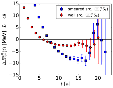
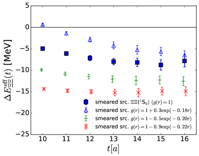
Figure 1: (Left) The source operator dependence of the effective energy shift $\Delta E_{\mathrm{eff}}(t)$ for $\Xi\Xi$ (¹S₀) using the wall source (red circles) and the smeared source (blue squares) for $L=48$ Iritani:2016jie . (Right) The sink operator dependence of the same quantity with the smeared source Iritani:2016jie .

In Ref. Iritani:2016jie , we pointed out that the plateau-like behaviors at $t\simeq 1$ fm in the direct method depend on sources or sink operators. For example, Fig. 1 (Left) shows the source operator dependence of the effective energy shift $\Delta E_{\mathrm{eff}}(t)$ in Eq. (3) for the $\Xi\Xi$ (¹S₀) on $L=48$, where $\mathcal{J}^{\rm sink}_{BB}(t)$ in Eq. (1) is given by

$$\mathcal{J}^{\rm sink}_{BB}(t) = \sum_{\vec{r}}\sum_{\vec{x}}B(\vec{x}+\vec{r},t)B(\vec{x},t),$$ (14)

where a baryon operator $B$ is given in Eq. (13). While plateau-like structures appear around $t/a\sim 15$ for both wall and smeared sources, the values disagree with each other. Similar inconsistencies are found on other volumes and the infinite volume extrapolation implies that the system is bound (unbound) for the smeared (wall) source. These discrepancies indicate some uncontrolled systematic errors. Indeed, such an early-time pseudo-plateau can be shown to appear even with 10% contamination of the excited states as demonstrated by the mockup data Iritani:2016jie .

Fig. 1 (Right) shows the sink operator dependence of $\Delta E_{\mathrm{eff}}(t)$ for $\Xi\Xi$ (¹S₀) with the smeared source fixed, where the sink operator is generalized as

$$\mathcal{J}^{\rm sink}_{BB}(t) = \sum_{\vec{r}}g(\vec{r})\sum_{\vec{x}}B(\vec{x}+\vec{r},t)B(\vec{x},t),$$ (15)

$$g(\vec{r}) = 1+\tilde{A}\exp(-\tilde{B}r),$$ (16)

with four different parameter sets, $(\tilde{A},\tilde{B})=(0.3,0.18),(-0.5,0.20),(-0.9,0.22)$ and $(0,0)$. The last one corresponds to the simple sink operator ($g(r)=1$) in Eq. (14). Although a plateau-like structure is observed for each sink operator, the values disagree with each other. This implies that the plateau-like behaviors at $t\simeq 1$ fm with the smeared source are not the plateau of the ground state but are pseudo-plateaux caused by contaminations of elastic scattering states other than the ground state. We note that such sink-operator dependence is not observed in the case of the wall source Iritani:2016jie .

3.2 Normality check

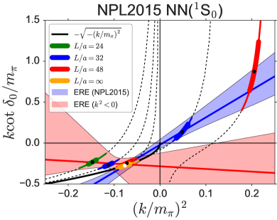
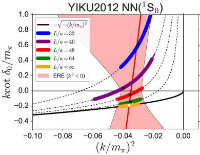
Figure 2: $k\cot\delta_{0}(k)/m_{\pi}$ as a function of $(k/m_{\pi})^{2}$ for $NN$(¹S₀) on each volume and the infinite volume in the direct method from Ref. Orginos:2015aya (Left) and Ref. Yamazaki:2012hi (Right). Black dashed lines correspond to Lüscher’s formula for each volume, while the black solid line represents the bound-state condition, $-\sqrt{-(k/m_{\pi})^{2}}$. The red line (with an error band) corresponds to the ERE obtained from the data at $k^{2}<0$ on finite volumes. In the left figure, the ERE fit to the data at $k^{2}>0$ on finite volumes together with only the infinite volume limit at $k^{2}<0$ is also shown by the blue line. Both figures from Ref. Iritani:2017rlk .

Since the information on operator dependence as shown in the previous subsection is not always available, we have introduced the “normality check” in Ref. Iritani:2017rlk , based on Lüscher’s finite volume formula together with the analytic properties of the $S$-matrix.

Some examples of the normality check are given in Fig. 2, where $k\cot\delta_{0}(k)$ is plotted as a function of $k^{2}$ for $NN$(¹S₀). Red and blue lines in Fig. 2 represent fits to data by the effective range expansion (ERE) at the next-to-leading order (NLO) as

$$k\cot\delta_{0}(k) = \frac{1}{a_{0}}+\frac{r_{0}}{2}k^{2},$$ (17)

where $a_{0}$ and $r_{0}$ are the scattering length and the effective range, respectively. In Fig. 2 (Left), inconsistency in ERE parameters is observed: The NLO ERE fit obtained from the data at $k^{2}<0$ on finite volumes (red line) disagrees with the fit to the data at $k^{2}>0$ on finite volumes together with the infinite volume limit at $k^{2}<0$ (blue line). For the latter fit (the blue line), the physical condition of the bound state pole is also violated. In Fig. 2 (Right), the NLO ERE fit exhibits a singular behavior as the divergent effective range. See Ref. Iritani:2017rlk for more detailed discussions.

As in the case of operator dependence, the normality check in Ref. Iritani:2017rlk indicates that the plateau fitting at $t\simeq 1$ fm suffers from large uncontrolled systematic errors probably due to contaminations from the excited states.

3.3 Source-operator dependence and derivative expansion of the potentials

In Ref. Iritani:2018zbt , we investigated source operator dependence of the potential as a tool to estimate the systematics associated with the derivative expansion of the HAL QCD potential, using two sources, wall and smeared sources.

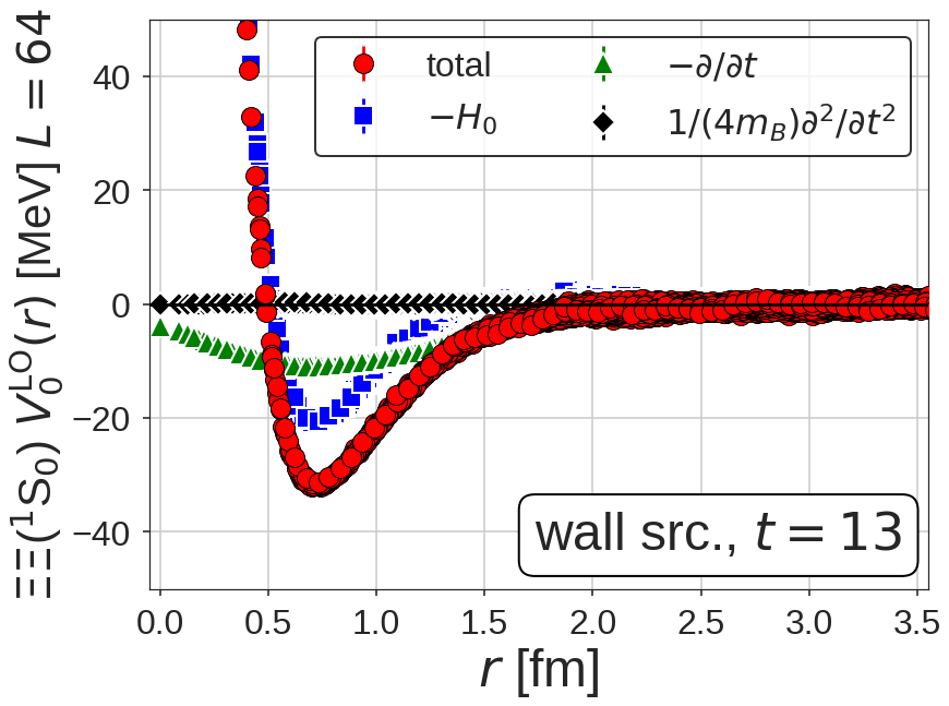
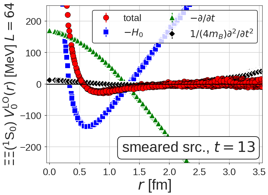
Figure 3: The potential at the leading order (LO) analysis $V_{0}^{\rm LO}(r)$ (red circles) from the wall source (Left) and the smeared source (Right) for $\Xi\Xi$(¹S₀) at $t/a=13$ for $L=64$ Iritani:2018zbt . The blue squares, green triangles and black diamonds denote 1st, 2nd and 3rd terms in Eq. (11), respectively.

Fig. 3 shows the LO $\Xi\Xi$(¹S₀) potential and its breakup into 1st, 2nd, and 3rd terms in Eq. (11) of the time dependent HAL QCD method from the wall source (Left) and the smeared source (Right). For the wall source, the 1st term dominates with moderate (negligible) contributions from the 2nd (3rd) term. As the 2nd term is not constant as a function of $r$, there exist small but non-negligible contributions from the excited states. For the smeared source, on the other hand, all terms are important. The substantial $r$ dependence of the 2nd term (green triangles), which indicates large contributions from the excited states in the smeared source, is canceled by the 1st term (blue squares) and further corrected by the 3rd term (black diamonds). The total potentials (red circles) from two sources, however, show qualitatively similar behaviors, which illustrates that the time-dependent HAL QCD method works well for extracting the potential irrespective of the source types.

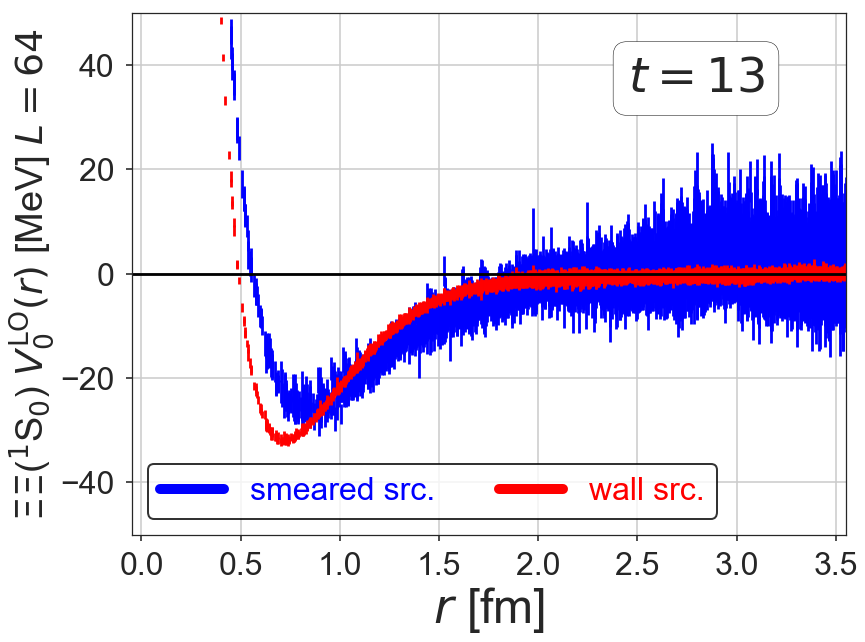
Figure 4: A comparison of the LO $\Xi\Xi$(¹S₀) potential $V_{0}^{\rm LO}(r)$ between the wall source (red) and the smeared source (blue) at $t/a=13$ Iritani:2018zbt .

Fig. 4 shows a comparison of the total potentials between two sources, $V_{0}^{\rm LO(wall/smear)}(r)$, at $t/a=13$. The potential approaches to zero within errors at larger $r$ for both sources, indicating that contributions from inelastic states are suppressed. While the potentials from two sources are very similar, there exists the non-zero difference between them. We find that this difference becomes smaller as $t$ increases, where the potential from the wall (smeared) source is independent of (dependent on) $t$ Iritani:2018zbt . This indicates that the effects of higher order terms in the derivative expansion exist in the data from the smeared source. Using the difference, $V_{0}^{\rm N^{2}LO}(r)$ and $V_{2}^{\rm N^{2}LO}(r)$ in Eq. (12) can be determined. In Fig. 5 (Left), $V_{0}^{\rm N^{2}LO}(r)$ together with $V_{0}^{\rm LO(wall)}(r)$ on $L=64$ at $t/a=13$ are plotted. As we find that $V_{0}^{\rm N^{2}LO}(r)$ agrees well with $V_{0}^{\rm LO(wall)}(r)$ except at short distances, we expect that $V_{0}^{\rm LO(wall)}(r)$ works well to reproduce physical observables at low energies. Indeed, as shown in Fig. 5 (Right), the N²LO correction to the S-wave scattering phase shift $\delta_{0}$ is small at low energies, showing not only that the derivative expansion converges well but also that the LO analysis for the wall source is sufficiently good at low energies.

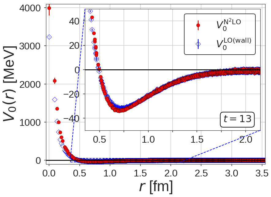
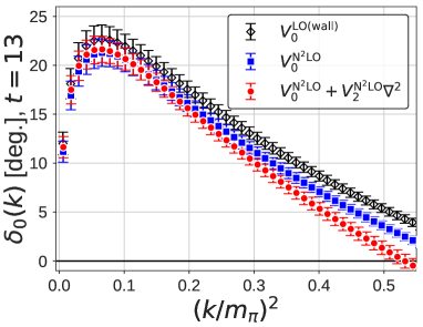
Figure 5: (Left) The LO $\Xi\Xi$(¹S₀) potential at the N²LO analysis, $V_{0}^{\mathrm{N^{2}LO}}(r)$ (red circles), together with the potential at the LO analysis for the wall source, $V_{0}^{\mathrm{LO(wall)}}(r)$ (blue diamonds) at $t/a=13$ on $L=64$. (Right) The scattering phase shifts $\delta_{0}(k)$ from $V_{0}^{\rm LO(wall)}$ (black diamonds), $V_{0}^{\rm N^{2}LO}(r)$ (blue squares) and $V_{0}^{\rm N^{2}LO}(r)+V_{2}^{\rm N^{2}LO}(r)\nabla^{2}$ (red circles) at $t/a=13$. Both figures from Ref. Iritani:2018zbt .

4 Anatomy: Excited state contaminations in the effective energy shifts

We now show our main results of this paper, where we analyze the behaviors of $\Xi\Xi$(¹S₀) temporal correlation functions for both wall and smeared sources using the HAL QCD potential and demonstrate that contaminations of elastic excited states cause pseudo-plateau behaviors at early time slices.

The strategy of our analysis is as follows. Provided that the leading order HAL QCD potential from the wall source is found to be a reasonable approximation of the exact potential, we evaluate eigenfunctions of the Hamiltonian with this potential in the finite box whose eigenvalues are below the inelastic threshold. We then calculate overlap factors between these eigenmodes and the $\Xi\Xi$ (¹S₀) correlation functions, in terms of which we reconstruct pseudo-plateau behaviors of the energy shifts. We also show that the plateaux of the temporal correlation functions projected to the lowest or the 2nd lowest eigenfunction agree with their eigenvalues. This fact demonstrates that both HAL QCD potential method and accurate extraction of energy shifts from the temporal correlation function give consistent results.

4.1 Eigenvalues and eigenfunctions in the finite box

We first evaluate eigenvalues and eigenfunctions of the leading-order HAL QCD Hamiltonian in a finite box given by

$$H^{\rm LO}=H_{0}+U,\qquad U\equiv V_{0}^{\rm LO(wall)},$$ (18)

where we take $V_{0}^{\rm LO(wall)}$ on each volume for $U$, since $V_{0}^{\rm LO(wall)}$ is a reasonable approximation of the exact potential $U$. Note that the volume dependence of $V_{0}^{\rm LO(wall)}$ is negligible, thanks to the short-ranged nature of the interaction.

In a finite lattice box, eigenvalues and eigenfunctions of the Hermitian matrix $H^{\rm LO}$ can be easily obtained. The $n$-th eigenvalue of $H^{\rm LO}$ in the $A_{1}^{+}$ representation below the inelastic threshold is tabulated in Table 2, where we show the energy shift compared to the threshold, $\Delta E_{n}\equiv W_{n}-2m_{\Xi}$. The number of excited states below the inelastic threshold is 3, 4 and 6 on $L=40$, 48, and 64, respectively. For larger volume, the energy gap becomes smaller and the number of elastic excited states increases.

$\Delta E_{n}$ [MeV]	$L=40$	$L=48$	$L=64$
$n=0$	$-5.5(1.0)\left({}^{+1.8}_{-0.4}\right)$	$-2.8(0.4)\left({}^{+1.1}_{-0.1}\right)$	$-1.5(0.3)\left({}^{+0.4}_{-0.1}\right)$
$n=1$	$77.2(0.8)\left({}^{+0.8}_{-4.7}\right)$	$52.0(0.4)\left({}^{+3.6}_{0.0}\right)$	$28.4(0.3)\left({}^{+0.4}_{-0.1}\right)$
$n=2$	$161.5(1.0)\left({}^{+0.2}_{-6.8}\right)$	$110.0(0.5)\left({}^{+3.2}_{0.0}\right)$	$60.4(0.4)\left({}^{+0.3}_{-0.1}\right)$
$n=3$	$236.5(1.1)\left({}^{+1.0}_{-0.7}\right)$	$164.9(0.6)\left({}^{+2.1}_{-0.5}\right)$	$93.2(0.4)\left({}^{+0.7}_{0.0}\right)$
$n=4$	—	$216.3(0.4)\left({}^{+1.0}_{-0.4}\right)$	$124.1(0.3)\left({}^{+0.2}_{-0.1}\right)$
$n=5$	—	—	$155.8(0.3)\left({}^{+0.6}_{-0.0}\right)$
$n=6$	—	—	$186.5(0.3)\left({}^{+0.8}_{0.0}\right)$

Table 2: Eigenvalues of the $n$-th eigenfunction below the inelastic threshold in the $A_{1}^{+}$ representation of the HAL QCD Hamiltonian $H^{\rm LO}$ in each volume. Eigenvalues are given in terms of the energy shifts from the threshold, $\Delta E_{n}\equiv W_{n}-2m_{\Xi}$. Central values and statistical errors are evaluated at $t/a=13$, while the systematic errors are estimated by using the results at $t/a=14,15,16$.

Fig. 6 shows the eigenfunctions $\Psi_{n}(\vec{r})$ on $L=48$, with $\sum_{\vec{r}}|\Psi_{n}(\vec{r})|^{2}=1$ and $\Psi_{n}(\vec{0})>0$. Up to a normalization, $\Psi_{n}(\vec{r})$ corresponds to the NBS wave function $\psi^{W=W_{n}}(\vec{r})$ in a finite volume. The lowest state $\Psi_{0}(\vec{r})$ has the similar shape to the $R$-correlator for the wall source, which shows a weak peak structure around $r\lesssim 1$ fm and becomes flat at large distances without any nodes, while the eigenfunctions for the excited states have nodes, whose number increases as the eigenvalue becomes larger. The short distance structures for $\Psi_{n>0}(\vec{r})$, which has a steeper peak around $r<1$ fm than that of $\Psi_{0}(\vec{r})$ resemble the $R$-correlator for the smeared source. Eigenfunctions on other volumes are collected in Appendix B.

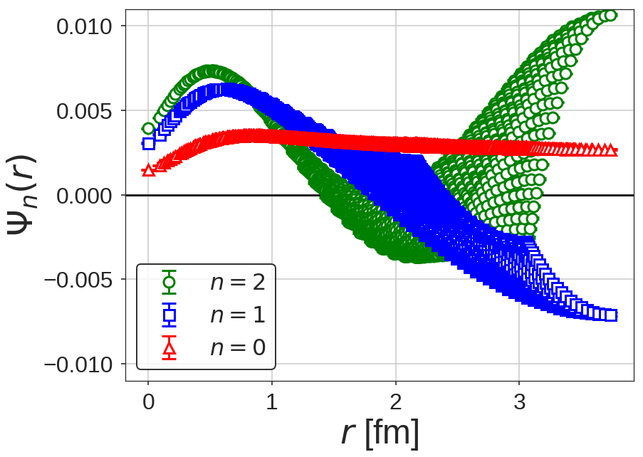
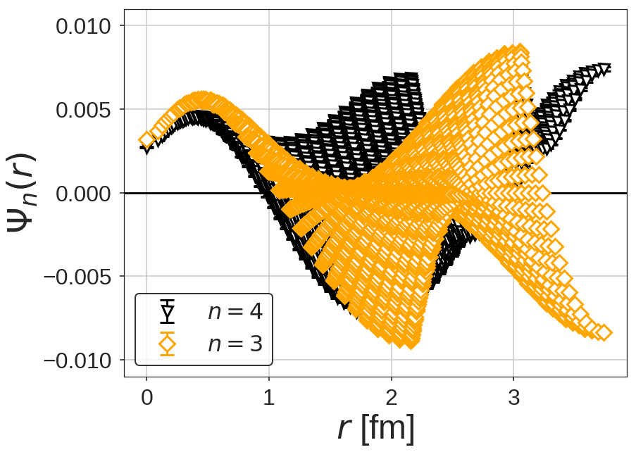
Figure 6: Eigenfunctions of elastic states in the $A_{1}^{+}$ representation of the HAL QCD Hamiltonian $H^{\rm LO}$ below the inelastic threshold $\Psi_{n}(\vec{r})$ on $L=48$ at $t/a=13$ for $n=0,1,2$ (Left) and $n=3,4$ (Right), where red up-pointing triangles, blue squares, green circles, orange diamonds and black down-pointing triangles correspond to $n=0,1,2,3$ and 4, respectively. The eigenfunction is normalized as $\sum_{\vec{r}}|\Psi_{n}(\vec{r})|^{2}=1$ and $\Psi_{n}(\vec{0})>0$. Errors are statistical only.

4.2 Decomposition of the $R$-correlator via eigenfunctions

Since the $R$-correlator is dominated by elastic states at moderately large $t$, we can expand it in terms of eigenfunctions of $H^{\mathrm{LO}}$ as

$$R^{\mathrm{wall/smear}}(\vec{r},t)=\sum_{n}a_{n}^{\mathrm{wall/smear}}\Psi_{n}(\vec{r})e^{-\Delta E_{n}t},$$ (19)

where the overlap coefficient $a_{n}$ characterizes the magnitude of the contribution from the corresponding eigenfunction. Using the orthogonality of $\Psi_{n}(\vec{r})$, $a_{n}$ can be determined by

$$a_{n}^{\mathrm{wall/smear}}=\sum_{\vec{r}}\Psi_{n}^{\dagger}(\vec{r})R^{\mathrm{wall/smear}}(\vec{r},t)e^{\Delta E_{n}t}.$$ (20)

The magnitude of the corresponding excited state contamination in the $R$-correlator is represented by the ratio $a_{n}/a_{0}$. In Fig. 7, we plot $a_{n}/a_{0}$ obtained at $t/a=13$ as a function of $\Delta E_{n}$ for the wall source (Left) and the smeared source (Right). Calculations at $t/a=14,15,16$ confirm that the results are almost independent of $t$ within statistical errors, indicating that the decomposition is reliable. In the case of the wall source, $R^{\mathrm{wall}}(r,t)$ has a large overlap with the ground state, and $|a_{n>0}/a_{0}|$ is smaller than 0.1. In the case of the smeared source, on the other hand, $|a_{n}/a_{0}|\sim\mathcal{O}(1)$ and thus all elastic excited states significantly contribute to the $R$-correlator.

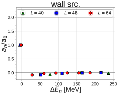
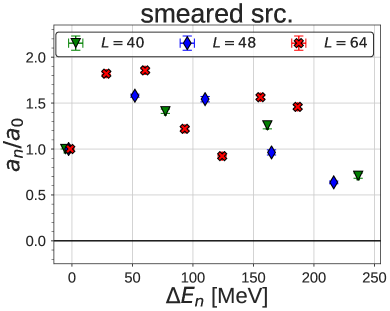
Figure 7: The ratio of the overlap coefficients $a_{n}/a_{0}$ in the $R$-correlator obtained at $t/a=13$ for the wall source (Left) and the smeared source (Right) on three volumes.

This difference of the magnitude in $a_{n}/a_{0}$ between two sources can be understood from the overlap between the $R$-correlator and the eigenfunctions. Fig. 8 shows the spatial profile of the overlap, $\Psi_{n}^{\dagger}(\vec{r})R(\vec{r},t)e^{\Delta E_{n}t}$, for the wall source (Left) and the smeared source (Right) on $L=48$, whose spatial summation corresponds to $a_{n}$. The contribution from the first excited state (blue squares) is highly suppressed for the wall source, thanks to the cancellation between positive values at short distances and negative values at long distances of $\Psi_{n=1}^{\dagger}(\vec{r})R^{\mathrm{wall}}(\vec{r},t)e^{\Delta E_{n=1}t}$. For the smeared source, on the contrary, the contamination from the 1st excited state remains non-negligible, due to the absence of the negative parts in $\Psi_{n=1}^{\dagger}(\vec{r})R^{\mathrm{smear}}(\vec{r},t)e^{\Delta E_{n=1}t}$.

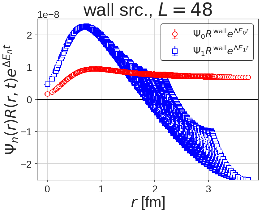
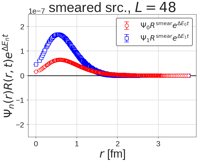
Figure 8: The overlap between the $R$-correlator and the eigenfunction, $\Psi_{n}^{\dagger}(\vec{r})R(\vec{r},t)e^{\Delta E_{n}t}$, as a function of $r$ at $t/a=13$ on $L=48$ for the ground state ($n=0$, red circles) and the first excited state ($n=1$, blue squares) in the case of the wall source (Left) and the smeared source (Right).

In the literature, the smeared source is often employed in the direct method, in order to suppress contributions from (inelastic) excited states in a “single-baryon” correlation function. The same smeared source, however, does not necessarily reduce the contaminations from the elastic excited states in the two-baryon correlation function, as is explicitly shown in Fig. 7. Indeed, one of the most relevant parameters which control the magnitudes of elastic state contributions is the relative distance $\vec{r}$ between two baryons at the source, which appears as

$$\frac{1}{L^{3}}\sum_{\vec{x}}B(\vec{x})B(\vec{x}+\vec{r})=\sum_{\vec{p}}\tilde{B}(\vec{p})\tilde{B}(-\vec{p})e^{i\vec{p}\cdot\vec{r}},\qquad\tilde{B}(\vec{p})\equiv\frac{1}{L^{3}}\sum_{\vec{x}}B(\vec{x})e^{-i\vec{p}\cdot\vec{x}}$$ (21)

in the center of mass system. Almost all literature of the direct method have employed the smeared source essentially corresponding to $|\vec{r}|=0$, which implies that elastic states for all $\vec{p}$ are equally generated at the source. Thus the choice $|\vec{r}|=0$ (or $|\vec{r}|\ll 1$) is one of the possible reasons for large contaminations from elastic excited states in the case of the smeared source. As long as $|\vec{r}|$ is non-zero and large, however, modes with non-zero $\vec{p}$ may be suppressed due to the oscillating factor $e^{i\vec{p}\cdot\vec{r}}$. The study in which the momentum projection is performed for each baryon in the source operator is recently reported in Ref. Francis:2018qch .

The temporal correlation function $R(t)$ is reconstructed in terms of eigenfunctions as

$$R^{\mathrm{wall/smear}}(t) = \sum_{\vec{r}}R^{\mathrm{wall/smear}}(\vec{r},t)=\sum_{\vec{r}}\sum_{n}a_{n}^{\mathrm{wall/smear}}\Psi_{n}(\vec{r})e^{-\Delta E_{n}t}=\sum_{n}b_{n}^{\mathrm{wall/smear}}e^{-\Delta E_{n}t},~{}~{}~{}~{}~{}~{}~{}$$ (22)

where $b_{n}\equiv a_{n}\sum_{\vec{r}}\Psi_{n}(\vec{r})$, whose ratio $b_{n}/b_{0}$ gives the magnitude of the contamination to $R(t)$ from the $n$-th elastic excited state.

Fig. 9 shows $|b_{n}/b_{0}|$ obtained at $t/a=13$ as a function of $\Delta E_{n}$ on three volumes for the wall source (Left) and the smeared source (Right). Solid (open) symbols correspond to positive (negative) values for $b_{n}/b_{0}$. For the wall source, the contamination from the first excited state is found to be smaller than 1%, and $|b_{n}/b_{0}|$ is further suppressed exponentially for higher excited states. In the case of the smeared source, the contamination from the first excited state is as large as $\sim 10$% with a negative sign and the contamination remains to be $\sim 1$% even for the higher excited state with $\Delta E_{n}\sim 100$ MeV.

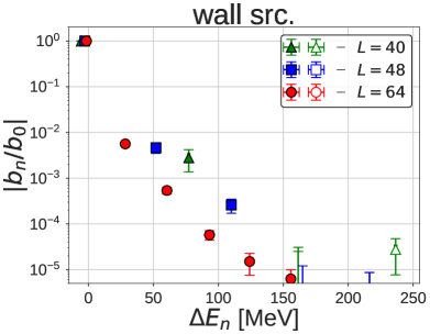
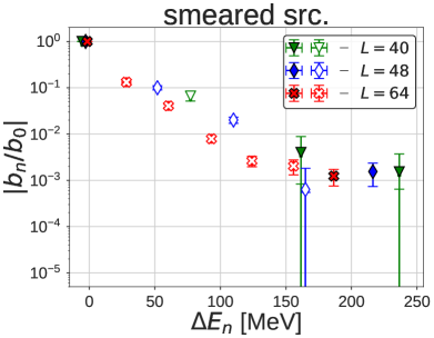
Figure 9: The ratio of the overlap coefficients in the temporal correlation function $|b_{n}/b_{0}|$ obtained at $t/a=13$ for the wall source (Left) and the smeared source (Right) on various volumes. Solid (open) symbols correspond to positive (negative) values of $b_{n}/b_{0}$.

4.3 Reconstruction of the effective energy shift

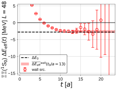
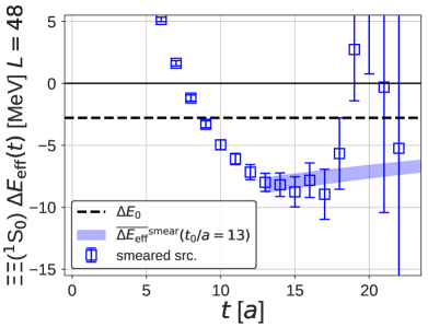
Figure 10: The reconstructed effective energy shifts $\overline{\Delta E}_{\mathrm{eff}}(t,t_{0}=13a)$ with statistical errors are plotted as a function of $t$ (colored bands), while the direct measurement of the effective energy shifts from $R$-correlators are plotted by red circles or blue squares. The black dashed lines correspond to the energy shift $\Delta E_{0}(t_{0}=13a)$ for the ground state of the HAL QCD Hamiltonian $H^{\rm LO}$ in the finite volume. The results on $L=48$ for the wall source (Left) and the smeared source (Right).

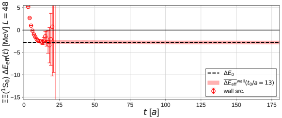
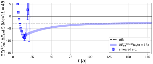
Figure 11: The same as Fig. 10 but for the wider range of the Euclidean time $t$.

Let us now examine the energy shifts obtained from the reconstructed $R$-correlators;

$$\overline{\Delta E}_{\mathrm{eff}}^{\mathrm{wall/smear}}(t,t_{0})=\frac{1}{a}\log\left[\frac{\displaystyle\sum_{n=0}^{n_{\mathrm{max}}}b_{n}^{\mathrm{wall/smear}}(t_{0})e^{-\Delta E_{n}(t_{0})t}}{\displaystyle\sum_{n=0}^{n_{\mathrm{max}}}b_{n}^{\mathrm{wall/smear}}(t_{0})e^{-\Delta E_{n}(t_{0})(t+a)}}\right],$$ (23)

where we take $n_{\mathrm{max}}=3$, 4, 6 for $L=40$, 48, 64, respectively, corresponding to the number of elastic excited states below the inelastic threshold, and $b_{n}(t_{0})$ and $\Delta E_{n}(t_{0})$ are extracted at fixed $t_{0}$.

In Fig. 10, we show the reconstructed effective energy shifts $\overline{\Delta E}_{\mathrm{eff}}(t,t_{0}=13a)$, together with numerical data of the effective energy shifts $\Delta E_{\mathrm{eff}}(t)$ from the $R$-correlators, for the wall source (Left) and the smeared source (Right) on $L=48$. The bands correspond to $\overline{\Delta E}_{\mathrm{eff}}(t,t_{0}=13a)$ with statistical errors coming from those of $b_{n}$ and $\Delta E_{n}$ at $t_{0}/a=13$, while red circles or blue squares correspond to $\Delta E_{\mathrm{eff}}(t)$ obtained directly from the $R$-correlator in Sec. 3.1. Here we do not consider $\overline{\Delta E}_{\mathrm{eff}}(t,t_{0}=13a)$ for $t/a<13$, where inelastic contributions are expected to be larger. Shown together by the black dashed line represents the energy shift $\Delta E_{0}(t_{0}=13a)$ for the ground state of the HAL QCD Hamiltonian $H^{\rm LO}$ on $L=48$.

We find that the results of the direct method, most notably the plateau-like structures around $t/a=15$, are well reproduced by $\overline{\Delta E}_{\mathrm{eff}}(t,t_{0})$ for both wall and smeared sources, indicating that the behaviors of $\Delta E_{\mathrm{eff}}(t)$ at this time interval in the direct method are explained by the contributions from the several low-lying states. These plateau-like structures, however, do not necessarily correspond to the plateau of the ground state. Indeed, in the case of the smeared source, there is a clear discrepancy between the value of the plateau-like structure and the eigenvalue $\Delta E_{0}$ of the ground state. This is a consequence of large excited state contaminations in the correlation function for the smeared source. In the case of the wall source, on the other hand, since the overlap with the ground state is large, the value of the plateau-like structure is consistent with the value $\Delta E_{0}$.

The fate of the plateau-like structures is more clearly seen in Fig. 11, where we plot the behaviors at asymptotically large $t$ of the reconstructed effective energy shifts $\overline{\Delta E}_{\mathrm{eff}}(t,t_{0}=13a)$ for the wall source (red band) and the smeared source (blue band). While the plateau-like structure at $t/a\sim 15$ for the wall source is almost unchanged at larger $t$, the value of $\overline{\Delta E}_{\mathrm{eff}}(t,t_{0}=13a)$ in the case of the smeared source gradually changes as $t$ increases until it reaches to the value of the ground state, $\Delta E_{0}$, at $t/a\sim 100$.

In Appendix D.1, we perform the same analysis on other volumes and observe essentially the same behaviors as in the case of $L=48$: For the wall source, the value of the plateau-like structure at $t/a\sim 15$ remains almost unchanged at larger $t$ and is consistent with $\Delta E_{0}$. For the smeared source, the value of the plateau-like structure at $t/a\sim 15$ is inconsistent with $\Delta E_{0}$. The deviation is found to be larger on a larger volume, due to severer contaminations from the excited states on larger volumes (See Sec. 4.2). The value of $\overline{\Delta E}_{\mathrm{eff}}(t,t_{0}=13a)$ for the smeared source gradually changes at $t$ increases and the ground state saturation is realized at $t/a\gtrsim 50,100$ and $150$ or $t\gtrsim 5,10$ and $15$ fm on $L=40,48$ and $64$, respectively. These time scales for the ground state saturation are actually not surprising but rather natural, considering the fact that the lowest excitation energy is as small as $\delta E\equiv\Delta E_{1}-\Delta E_{0}\simeq 84$, 55 and 30 MeV on $L=40$, 48 and 64, respectively.

These results clearly reveal that the plateau-like structures at $t/a\sim 15$ for the smeared source are pseudo-plateaux caused by contaminations of the elastic excited states. While the effective energy shifts from the wall source happen to be saturated by the ground state even at $t/a\sim 15$, it is generally difficult to confirm that a plateau-like structure corresponds to the correct energy shift of the ground state without the help of other inputs, such as the HAL QCD potential analysis in the present case. Since the calculation of the energy shift from the $R$-correlator at $t\sim(\delta E)^{-1}$ is impractical due to the exponentially growing noises, one cannot obtain the correct spectra from the plateau identification in the direct method unless sophisticated variational techniques Luscher:1990ck are employed.

4.4 Projection with improved sink operator

Once the finite-volume eigenmodes of $H^{\rm LO}$ with the HAL QCD potential are known, an improved two-baryon sink operator for a designated eigenstate can be constructed as

$$\mathcal{J}_{BB}^{\rm sink}(t) = \sum_{\vec{r}}\Psi_{n}^{\dagger}(\vec{r})\sum_{\vec{x}}B(\vec{x}+\vec{r},t)B(\vec{x},t),$$ (24)

which is expected to have a large overlap to the $n$-th elastic state. This is equivalent to considering the generalized temporal correlation function with the choice of $g(\vec{r})=\Psi_{n}^{\dagger}(\vec{r})$ in Eq. (15),

$$R^{(n)}(t) \equiv \sum_{\vec{r}}\Psi_{n}^{\dagger}(\vec{r})R(\vec{r},t),$$ (25)

from which we define the effective energy shift for the $n$-th eigenfunction as

$$\Delta E_{\mathrm{eff}}^{(n)}(t)=\frac{1}{a}\log\frac{R^{(n)}(t)}{R^{(n)}(t+a)}.$$ (26)

Fig. 12 shows the effective energy shift $\Delta E_{\mathrm{eff}}^{(n)}(t)$ using the wall source (black up-triangles) and the smeared sources (purple down-triangles) on $L=48$ for the ground state (Left) and the first excited state (Right). Shown together are the energy shift ($\Delta E_{0}$ or $\Delta E_{1}$) with statistical errors (red bands), obtained from $H^{\rm LO}$ with the HAL QCD potential $V_{0}^{\mathrm{LO(wall)}}(r)$ at $t/a=13$, as well as that for a non-interacting system (black lines). In the case of the ground state (Fig. 12 (Left)), the effective energy shifts from the direct method for the wall source (red circles) and the smeared source (blue squares) are also plotted for comparisons.

Figure 12: The effective energy shift $\Delta E_{\mathrm{eff}}^{(n)}(t)$ on $L=48$ from the wall source (black up triangles) and the smeared source (purple down triangles) for the ground state (Left) and the first excited state (Right). Red bands represent the energy shifts with statistical errors obtained from the HAL QCD Hamiltonian $H^{\rm LO}$, while black lines represent those for a non-interacting system. In the left figure, the effective energy shifts in the direct method for the wall source (red circles) and the smeared source (blue squares) are also shown.

First of all, after the sink projections, the results with the wall source and those with the smeared source agree well around $t/a\sim 13$ not only for the ground state but also for the first excited state. This is in sharp contrast with the fact that the results in the direct method without projections disagree between two sources for the ground state. Although a small overlap with the first excited state causes relatively large statistical errors in the case of the wall source, an agreement between two sources for the first excited states is rather striking, and serves as a non-trivial check for the reliability of the effective energy shifts with the sink projection. Moreover, results after the sink projections also agree with those from the HAL QCD Hamiltonian. Although the sink projection utilizes the information of the HAL QCD potential through eigenfunctions, agreements in effective energy shifts within statistical errors for both ground and first excited states provide a non-trivial consistency check between the HAL QCD method and the direct method with proper projection. In other words, results in Fig. 12 establish that (i) the HAL QCD potential correctly describes the energy shifts of two baryons in the finite volume for both ground and excited states, and that (ii) these energy shifts can also be extracted in the direct method if and only if interpolating operators are highly improved. Since the origins of systematic uncertainties are generally quite different between the two methods, such a “projection check” would be useful in future lattice QCD studies for two-baryon systems.

In recent years, it has been argued that seemingly inconsistent results for the $NN$ systems at heavy pion masses between Lüscher’s finite volume method and the HAL QCD method may indicate some theoretical deficits in one of the two methods. It is now clear from our analysis that Lüscher’s method and the HAL QCD method agree quantitatively with each other, as it should be so theoretically.

5 Summary

In our previous works Iritani:2016jie ; Iritani:2017rlk , it has been shown that the plateau fitting of the eigenenergies at early Euclidean times $t$, employed in the direct method, is generally unreliable for multi-baryon systems, due to the appearance of pseudo-plateaux caused by contaminations of the excited states with small gap corresponding to the elastic scattering states on the finite volume. In this paper, we quantified the degree of contaminations from such excited states by decomposing the two-baryon correlation functions in terms of the finite-volume eigenmodes of the HAL QCD Hamiltonian.

By taking $\Xi\Xi$ (¹S₀) system at $m_{\pi}=0.51$ GeV in (2+1)-flavor lattice QCD with the wall and smeared quark sources for $La=3.6,4.3,5.8$ fm, we showed that the excited state contaminations are suppressed for the wall source, while those for the smeared source are substantial and become severer on a larger spatial extent. For the smeared source, the plateau-like structures at $t=1\sim 2$ fm are shown to be pseudo-plateaux and the plateau with the ground state saturation is realized only at $t>5\sim 15$ fm corresponding to the inverse of the lowest excitation energy. We also demonstrated that one can optimize the two-baryon operator utilizing the finite-volume eigenmode of the HAL QCD Hamiltonian. The effective energies from the temporal correlation functions with the optimized operators are found to be consistent with the finite volume spectra obtained from the HAL QCD Hamiltonian. This result establishes not only that the correct finite-volume spectra can be accessed by employing highly optimized operators even in the direct method but also that the HAL QCD method and the direct method agree in the finite volume spectra for the two baryon systems. Thus the long-standing issue on the consistency between Lüscher’s finite volume method and the HAL QCD method is positively resolved at least for the particular system considered here. The next step is to carry out comprehensive studies of baryon-baryon interactions around the physical quark masses in the HAL QCD method, which are partly underway (see, e.g. Gongyo:2017fjb ; Iritani:2018sra ; Inoue:2018axd ). Those will reveal not only the nature of exotic dibaryons but also the equation of state of dense baryonic matter.

Appendix A The finite volume spectra from the N²LO potential

In the main text (Sec. 4), we study the finite volume spectra to be used for the spectral decomposition of the $R$-correlator using the LO potential. In this appendix, we employ the potential at the N²LO analysis (Eq. (12)) and examine a stability of the finite volume spectra against the order of the derivative expansion. The HAL QCD Hamiltonian with the N²LO potential is given by

$$H^{\mathrm{N^{2}LO}}=H_{0}+V_{0}^{\mathrm{N^{2}LO}}(r)+V_{2}^{\mathrm{N^{2}LO}}(r)\nabla^{2}.$$ (27)

Note that, while $H$ is non-Hermitian, its eigenenergies are real since the eigen equation can be rewritten as the definite generalized Hermitian eigenvalue problem Iritani:2018zbt . The eigenenergies at $L=64$ using $V_{0}^{\mathrm{LO(wall)}}$, $V_{0}^{\mathrm{N^{2}LO}}$, and $V_{0}^{\mathrm{N^{2}LO}}+V_{2}^{\mathrm{N^{2}LO}}\nabla^{2}$ are summarized in Table 3. The results from the different potentials are consistent with each other at low energies within statistical errors and the N²LO correction remains to be small (at most $\sim 1$% difference) even for higher energies. These results are in line with the observation that the LO analysis from the wall source gives the correct phase shifts at low energies and the N²LO analysis gives only small correction even at higher energies Iritani:2018zbt .

$\Delta E_{n}$ [MeV]	$V_{0}^{\mathrm{LO(wall)}}$	$V_{0}^{\mathrm{N^{2}LO}}$	$V_{0}^{\mathrm{N^{2}LO}}+V_{2}^{\mathrm{N^{2}LO}}\nabla^{2}$
$n=0$	-1.5(0.3)	-1.4(0.3)	-1.4(0.3)
$n=1$	28.4(0.3)	28.6(0.3)	28.7(0.3)
$n=2$	60.4(0.4)	60.8(0.4)	61.2(0.4)
$n=3$	93.2(0.4)	93.4(0.4)	93.7(0.4)
$n=4$	124.1(0.3)	124.3(0.3)	124.6(0.3)
$n=5$	155.8(0.3)	156.5(0.3)	157.7(0.4)
$n=6$	186.5(0.3)	187.3(0.3)	189.1(0.4)

Table 3: The finite volume spectra using $V_{0}^{\mathrm{LO(wall)}}$, $V_{0}^{\mathrm{N^{2}LO}}$, and $V_{0}^{\mathrm{N^{2}LO}}+V_{2}^{\mathrm{N^{2}LO}}\nabla^{2}$ at $L=64$ evaluated at $t/a=13$.

Appendix B Eigenfunctions on various volumes

In this appendix, we show the shapes of eigenfunctions on various volume.

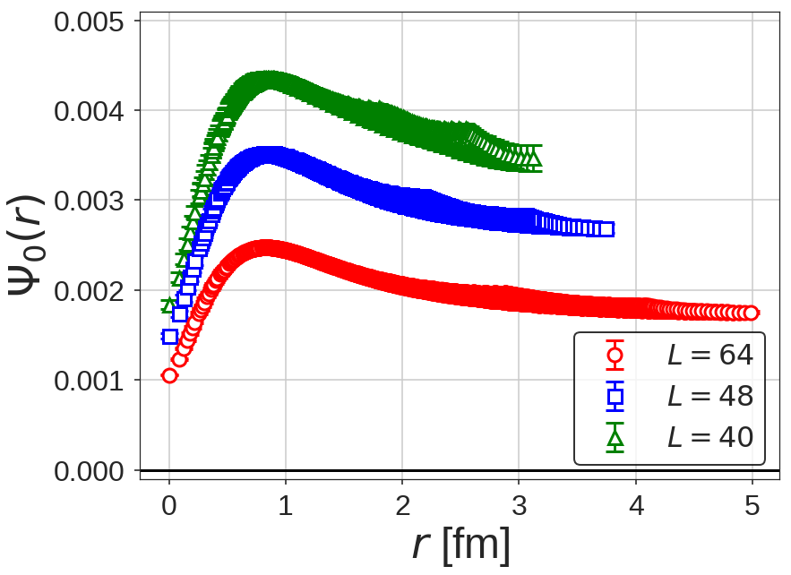
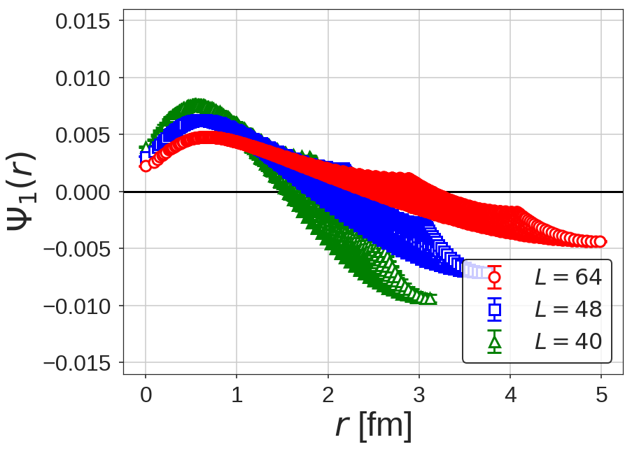
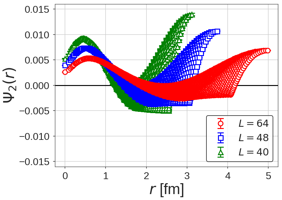
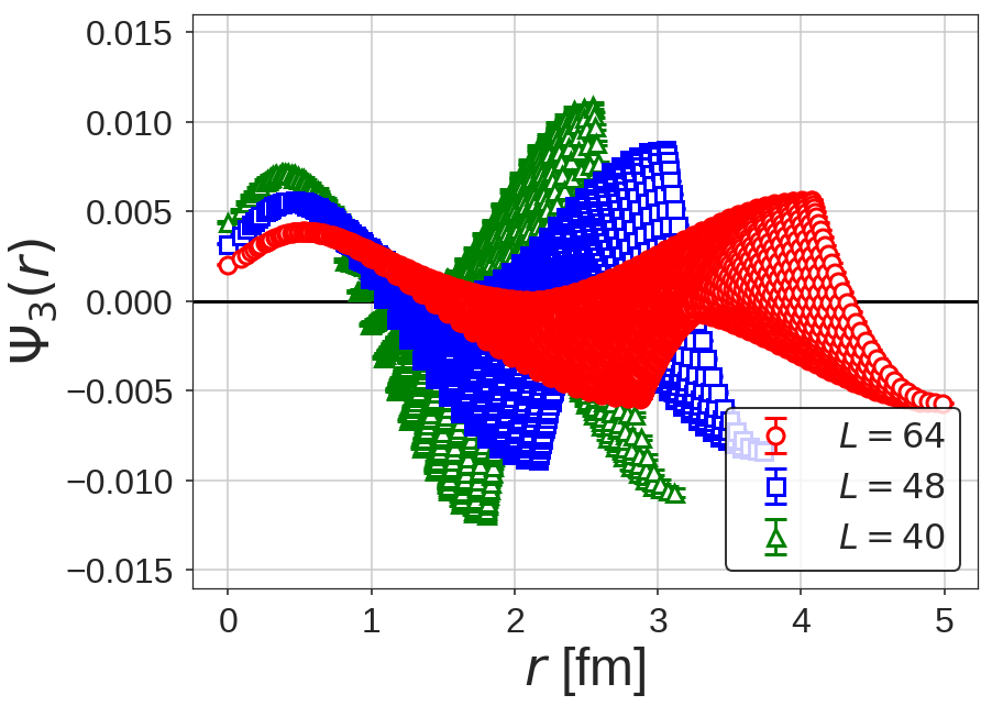
Figure 13: The low-lying eigenfunctions $\Psi_{n}(\vec{r})$ in the $A_{1}^{+}$ representation of the HAL QCD Hamiltonian with $V_{0}^{\mathrm{LO(wall)}}$ at $t/a=13$ for $L=40,48$ and 64. The top-left, top-right, bottom-left, bottom-right figure corresponds to $n=0,1,2,3$, respectively. The eigenfunction is normalized as $\sum_{\vec{r}}|\Psi_{n}(\vec{r})|^{2}=1$ and its sign is fixed to satisfy $\Psi_{n}(\vec{0})>0$.

Appendix C Reconstruction of the $R$-correlator

In this appendix, we study how good the original $R$-correlator $R(\vec{r},t)$ is approximated by the reconstructed $R$-correlator $\overline{R}(\vec{r},t)$ given by

$$\overline{R}(\vec{r},t)=\sum_{n=0}^{n_{\mathrm{max}}}a_{n}\Psi_{n}(r)e^{-\Delta E_{n}t},$$ (28)

where $n_{\mathrm{max}}=3$, 4, 6 for $L=40$, 48, 64, corresponding to the number of excited elastic states below the inelastic threshold. Fig. 14 shows the comparison between the original (red squares) and the reconstructed (blue circles) $R$-correlators for the wall source (Left) and the smeared source (Right) at $t/a=13$. Shown together by black diamonds are the difference between the two, $R(\vec{r},t)-\overline{R}(\vec{r},t)$. To estimate the magnitude of the difference, we define the residual norm by

$$\frac{\sum_{\vec{r}}|R(\vec{r},t)-\overline{R}(\vec{r},t)|^{2}}{\sum_{\vec{r}}|R(\vec{r},t)|^{2}},$$ (29)

whose values are also shown in the panels in Fig. 14.

In the case of the wall source, it is found that the reconstruction works very well and the residuals are negligible ($\lesssim 10^{-5}$). In the case of the smeared source, while the reconstruction is not as perfect as in the case of the wall source, the reconstructed $R$-correlator well reproduces the overall behavior of the original one where the residuals are only $\sim 0.4-5\%$. The main origin of the residuals is the small discrepancies at short distances which become more apparent for a larger volume. This indicates that there remain small contributions from excited states above inelastic threshold in the case of the smeared source. In fact, since all elastic states couple to the smeared source with the same order of magnitude (See Fig. 7), there could remain contributions from elastic as well as inelastic states above the threshold for $R(\vec{r},t)$ even at $t/a=13$, whose magnitude is expected to be larger for a larger volume due to the larger density of states.

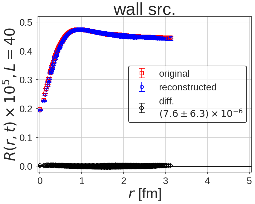
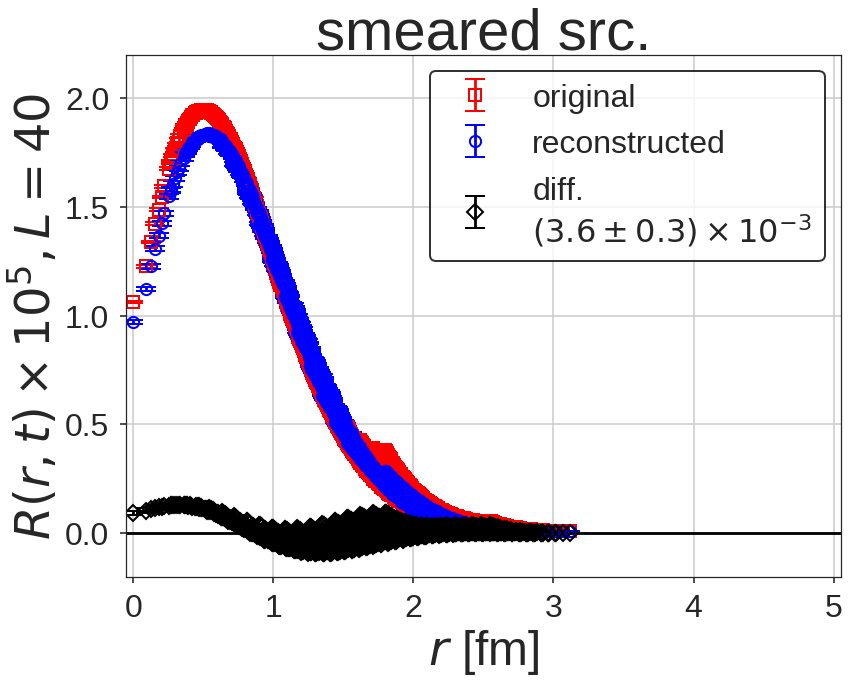
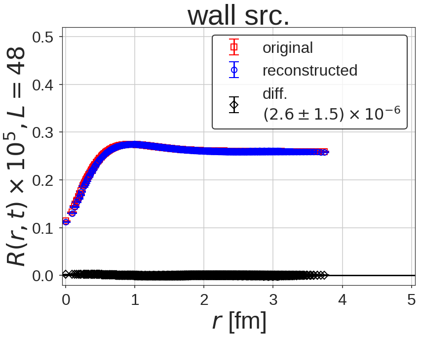
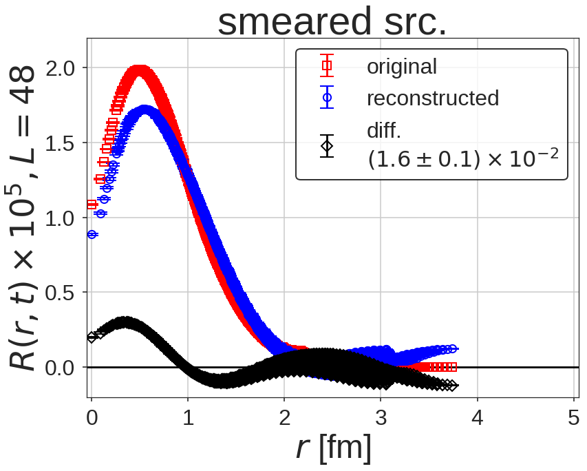
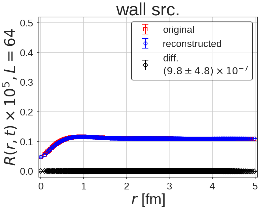
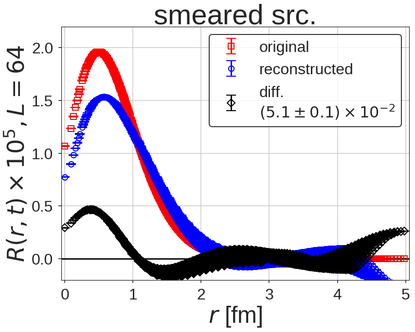
Figure 14: Comparisons between the original $R$-correlator (red squares) and the reconstructed $R$-correlator using low-lying eigenstates below the inelastic threshold (blue circles) at $t/a=13$ for $L=40$ (top), 48 (middle), 64 (bottom). The differences between the two $R$-correlators are shown by black diamonds and the values for the corresponding residual norms are given in legend panels. (Left) The wall source. (Right) The smeared source.

Appendix D Reconstructed effective energy shifts

We collect the results on the reconstructed effective energy shifts, Eq. (23).

D.1 The results on various volumes

As shown in Fig. 15, we observe that the reconstruction generally works well. A small deviation at early time slices on $L=64$ for the smeared source is most likely due to the statistical fluctuations and/or the systematics due to contaminations from the states above the threshold discussed in Appendix C.

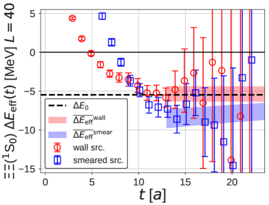
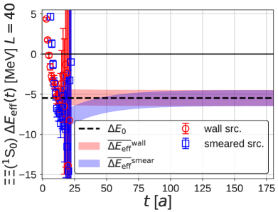
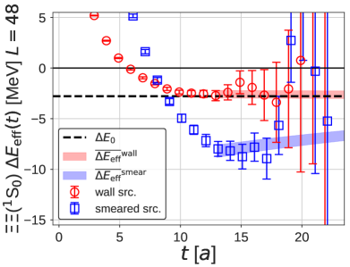
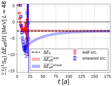
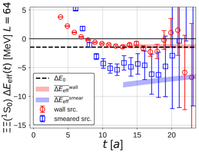
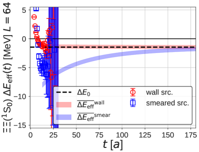
Figure 15: The reconstructed effective energy shifts $\overline{\Delta E_{\mathrm{eff}}}(t,t_{0}=13a)$ for the wall source (red bands) and the smeared source (blue bands) at $L=40$, 48 and 64. The effective energy shifts in the direct method are also shown for the wall (red circles) and smeared (blue squares) sources. The black dashed lines are the energy shifts for the ground state of the HAL QCD Hamiltonian in the finite volume evaluated at $t_{0}/a=13$. (Left) $0\leq t/a\leq 24$. (Right) $0\leq t/a\leq 175$.

D.2 Contributions from excited states to the effective energy shifts

We study how each elastic excited state contributes to the effective energy shift for the smeared source, by changing the number of elastic excited states used in the reconstruction ($n_{\mathrm{max}}$) in Eq. (23).

Fig. 16 shows the $n_{\mathrm{max}}$ dependence of the reconstructed effective energy shifts for the smeared source at $L=40$, $48$ and $64$, which are compared with the lowest eigenenergies $\Delta E_{0}$ (red bands). Due to the negative sign of $b_{n}/b_{0}<0$ (see Fig. 9 (Right)), the reconstructed effective energy shifts are smaller than $\Delta E_{0}$. For $L=40$ and 48, the dominant contribution comes from the first excited state ($n_{\mathrm{max}}=1$) besides the ground state and higher modes give only minor corrections, while the second excited state ($n_{\mathrm{max}}=2$) also gives significant contribution for $L=64$. These results indicate that the pseudo-plateau structures around $t/a\sim 15$ are originated mostly from the scattering states below $\sim 90$ MeV (See Table 2).

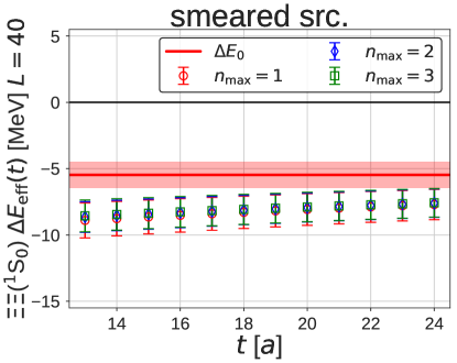
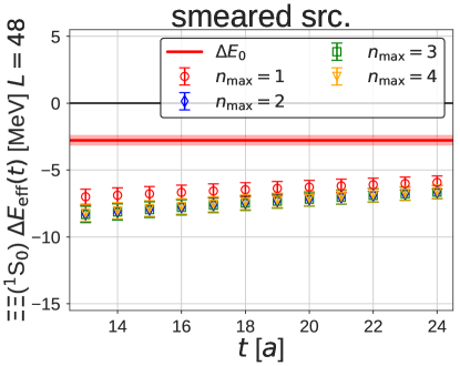
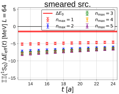
Figure 16: The mode number ($n_{\mathrm{max}}$) dependence of the reconstructed effective energy shift $\overline{\Delta E_{\mathrm{eff}}}(t,t_{0}=13a)$ for the smeared source at $L=40$ (top), $48$ (middle) and $64$ (bottom).

Appendix E Effective energy shifts from the improved sink operator based on eigenfunctions

In this appendix, we present effective energy shifts on various volumes, which are obtained from the improved two-baryon sink operator, projected to the ground state/first excited state in Eq. (24). Results are found to be consistent with the corresponding finite-volume eigenenergies of the HAL QCD Hamiltonian. Small discrepancies for the smeared source on $L=64$ are most likely due to the statistical fluctuations and/or the systematics due to contaminations from the states above the threshold discussed in Appendix C. Shown together in the left figure are the effective energy shifts in the direct method (without projection), where the significant deviation is observed for the smeared source.

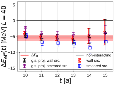
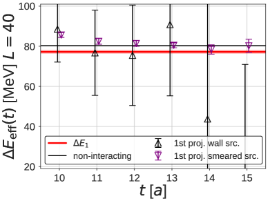
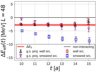
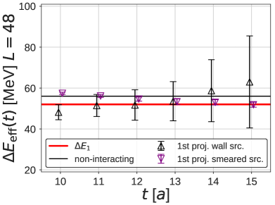
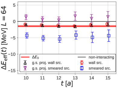
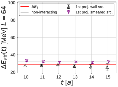
Figure 17: Same as Fig. 12 on $L=40$ (top), $48$ (middle) and 64 (bottom).

References

- (1) T. Iritani et al. [HAL QCD Collaboration], JHEP 1610, 101 (2016) [arXiv:1607.06371 [hep-lat]].
- (2) T. Iritani et al., Phys. Rev. D 96, 034521 (2017) [arXiv:1703.07210 [hep-lat]].
- (3) T. Yamazaki, K. i. Ishikawa, Y. Kuramashi and A. Ukawa, Phys. Rev. D 92, 014501 (2015) [arXiv:1502.04182 [hep-lat]], and references therein.
- (4) M. L. Wagman, F. Winter, E. Chang, Z. Davoudi, W. Detmold, K. Orginos, M. J. Savage and P. E. Shanahan, Phys. Rev. D 96, 114510 (2017) [arXiv:1706.06550 [hep-lat]], and references therein.
- (5) E. Berkowitz, T. Kurth, A. Nicholson, B. Joo, E. Rinaldi, M. Strother, P. M. Vranas and A. Walker-Loud, Phys. Lett. B 765, 285 (2017) [arXiv:1508.00886 [hep-lat]], and references therein.
- (6) M. Lüscher, Commun. Math. Phys. 104, 177 (1986); ibid., 105, 153 (1986).
- (7) M. Lüscher, Nucl. Phys. B 354, 531 (1991).
- (8) N. Ishii, S. Aoki and T. Hatsuda, Phys. Rev. Lett. 99, 022001 (2007) [arXiv:nucl-th/0611096].
- (9) S. Aoki, T. Hatsuda and N. Ishii, Prog. Theor. Phys. 123, 89 (2010) [arXiv:0909.5585 [hep-lat]].
- (10) N. Ishii et al. [HAL QCD Collaboration], Phys. Lett. B712, 437 (2012).
- (11) S. Aoki et al. [HAL QCD Collaboration], Prog. Theor. Exp. Phys. 2012, 01A105 (2012) [arXiv:1206.5088 [hep-lat]].
- (12) S. Aoki, in Les Touches 2009 “Modern Perspective in Lattice QCD: Quantum Field Theory and High Performance Computing”, p.591-p.628, ed. L. Lellouch, R. Sommer, B. Svetisky, A. Vladikas, L. F. Cugliandolo, Oxford University Press, 2011 [arXiv:1008.4427 [hep-lat]].
- (13) S. R. Beane et al. [NPLQCD Collaboration], Phys. Rev. D 87, 034506 (2013) [arXiv:1206.5219 [hep-lat]].
- (14) T. Inoue et al. [HAL QCD Collaboration], Nucl. Phys. A 881, 28 (2012) [arXiv:1112.5926 [hep-lat]].
- (15) A. Francis, J. R. Green, P. M. Junnarkar, C. Miao, T. D. Rae and H. Wittig, arXiv:1805.03966 [hep-lat].
- (16) T. Iritani [HAL QCD Collaboration], PoS LATTICE 2016, 107 (2016) [arXiv:1610.09779 [hep-lat]].
- (17) S. Aoki, T. Doi and T. Iritani, EPJ Web Conf. 175, 05006 (2018) [arXiv:1707.08800 [hep-lat]].
- (18) T. Iritani [HALQCD Collaboration], EPJ Web Conf. 175, 05008 (2018) [arXiv:1710.06147 [hep-lat]].
- (19) T. Iritani et al. [HALQCD Collaboration], Phys. Rev. D 99, 014514 (2019) [arXiv:1805.02365 [hep-lat]].
- (20) G. Parisi, Phys. Rept. 103, 203 (1984). doi:10.1016/0370-1573(84)90081-4
- (21) G. P. Lepage, CLNS-89-971, in From Actions to Answers: Proceedings of the TASI 1989, edited by T. Degrand and D. Toussaint (World Scientific, Singapore, 1990).
- (22) See, e.g., Wikipedia: https://en.wikipedia.org/wiki/Sanity_check
- (23) K. Murano, N. Ishii, S. Aoki and T. Hatsuda, Prog. Theor. Phys. 125, 1225 (2011) [arXiv:1103.0619 [hep-lat]].
- (24) K. Nishijima, Phys. Rev. 111, 995 (1958); W. Zimmermann, Nuovo Cim. 10, 597 (1958); R. Haag, Phys. Rev. 112, 669 (1958)
- (25) T. Yamazaki, K. i. Ishikawa, Y. Kuramashi and A. Ukawa, Phys. Rev. D 86, 074514 (2012) [arXiv:1207.4277 [hep-lat]].
- (26) T. Doi and M. G. Endres, Comput. Phys. Commun. 184, 117 (2013) [arXiv:1205.0585 [hep-lat]].
- (27) K. Orginos, A. Parreno, M. J. Savage, S. R. Beane, E. Chang and W. Detmold, Phys. Rev. D 92, 114512 (2015) [arXiv:1508.07583 [hep-lat]].
- (28) S. R. Beane et al., arXiv:1705.09239 [hep-lat].
- (29) M. Lüscher and U. Wolff, Nucl. Phys. B 339, 222 (1990).
- (30) R. A. Briceno, J. J. Dudek and R. D. Young, Rev. Mod. Phys. 90, 025001 (2018) [arXiv:1706.06223 [hep-lat]], and references therein.
- (31) S. Gongyo et al. [HAL QCD Collaboration], Phys. Rev. Lett. 120, 212001 (2018) [arXiv:1709.00654 [hep-lat]].
- (32) T. Iritani et al. [HAL QCD Collaboration], arXiv:1810.03416 [hep-lat].
- (33) T. Inoue [HAL QCD Collaboration], arXiv:1809.08932 [hep-lat].
- (34) T. Amagasa et al., J. Phys. Conf. Ser. 664, 042058 (2015).
- (35) http://www.lqcd.org/ildg, http://www.jldg.org
- (36) Columbia Physics System (CPS), http://usqcd-software.github.io/CPS.html
- (37) Bridge++, http://bridge.kek.jp/Lattice-code/
- (38) M. Schröck and H. Vogt, Comput. Phys. Commun. 184, 1907 (2013) [arXiv:1212.5221 [hep-lat]].
- (39) T. Boku et al., PoS LATTICE 2012, 188 (2012) [arXiv:1210.7398 [hep-lat]].
- (40) M. Terai et al., “Performance Tuning of a Lattice QCD code on a node of the K computer,” IPSJ Transactions on Advanced Computing Systems, Vol.6 No.3 43-57 (Sep. 2013) (in Japanese).