HUB-EP-99/67

QCD forces and heavy quark bound states

Abstract

The present knowledge of QCD confining forces between static test charges is summarised, with an emphasis on lattice results. Recent developments in relating QCD potentials to quarkonium properties by use of effective field theory methods are presented. The validity of non-relativistic QCD and the adiabatic approximation with respect to heavy quark bound states is explored. Besides the static potential and relativistic correction terms, the spectra of glueballs and gluinoballs, hybrid excitations of the QCD flux tube between fundamental colour sources, potentials between charges in various representations of the $SU(3)$ gauge group, and multi-particle interactions are discussed. Some implications for quarkonia systems and quark-gluon hybrid mesons are drawn.

1 Motivation

The phenomenology of strong interactions contains three fundamental ingredients: the confinement of colour charges, chiral symmetry breaking and asymptotic freedom. The latter requirement culminated in the invention of quantum chromodynamics (QCD) some 25 years ago. Predicting low energy properties of strongly interacting matter still represents a serious theoretical challenge. This is particularly disappointing since non-perturbative techniques are not only important in QCD but also for an understanding of physics beyond the standard model or perturbation theory. For instance a rigorous proof is still lacking that shows QCD as the microscopic theory of strong interactions to give rise to the macroscopic properties of chiral symmetry breaking and quark confinement.

So far Lattice Gauge Theory [1] constitutes the only known entirely non-perturbative regularisation scheme. By numerically simulating gauge theories on a lattice, one can in principle predict properties of interacting QCD matter without any non-QCD input (except for the quark masses). Such simulations have provided convincing evidence not only for quark confinement [2] but also for chiral symmetry breaking. Moreover, at finite temperature, pure gauge theories are found to undergo a confinement-deconfinement phase transition [3, 4, 5] while chiral symmetry is restored at high temperature [6, 7], in QCD with sea quarks. The accuracy of these results has been tremendously improved during the past decade with the availability of more powerful computers and advanced numerical techniques.

Unfortunately, the speed and memory of present day computers still allows only for “solving” relatively simple QCD problems to a satisfactory precision. One particular weakness that the standard lattice methodology shares with, for instance, the QCD sum rule approach [8, 9] is the difficulty in calculating properties of radially excited hadrons. In simple potential models, however, the spectrum of such excitations can easily be computed. Such models have been successfully applied in quarkonium physics since the discovery of the $J/\psi$ resonance more than two decades ago [10, 11, 12, 13, 14, 15, 16, 17, 18, 19, 20, 21].

A Hamiltonian representation in terms of functions of simple dynamical variables such as distance, angular momentum, relative momentum and spin allows for an understanding of the underlying system that is rather transparent and intuitive. One would like to clarify what component of the success of this simple picture results from the freedom of choice in constructing a phenomenological Hamiltonian and what part indeed reflects fundamental properties of the underlying bound state dynamics. Not long ago, a semi-relativistic Hamiltonian that governs heavy quarkonia bound states has been directly derived from QCD [22, 23, 24, 25, 26, 27, 28, 29, 30, 31, 32]. Starting from a non-relativistic expansion of the QCD Lagrangian (NRQCD) [33, 34, 35], the gluonic degrees of freedom have been separated from the heavy quark dynamics into functions of the canonical coordinates (the potentials) and integrated out by means of lattice simulations [29]. The resulting Hamiltonian incorporates many properties of the previously proposed purely phenomenological or QCD inspired models.

Heavy quarks closely resemble static test charges which can be used to probe microscopic properties of the QCD vacuum, in particular the anatomy of the confinement mechanism. Indeed, from charmonium spectroscopy and even more so from bottomonia states, a lot has been learned about the nature and properties of QCD confining forces. Either motivated by experimental input or by QCD itself, many effective models of low energy aspects have been proposed, in particular bag models [36, 37, 38, 39, 40], strong coupling and flux tube models [41, 42, 43, 44], bosonic string models [45, 46, 47], the stochastic vacuum model [48, 49, 50], dual QCD [51, 52, 53, 54] and the Abelian Higgs model [55], instanton based models [56, 57, 58] and relativistic quark models [59]. Many of these models are either expected to apply best to a non-relativistic setting or can most easily be solved in the situation of slowly moving colour charges.

In view of the fact that many problems like properties of complex nuclei are unlikely ever to be solved from first principles alone, to some extent modelling and approximations will always be required. Recently, using the stochastic vacuum model as well as dual QCD and the minimal area law, that is common to the strong coupling limit and string pictures, the potentials within the quarkonium bound state Hamiltonian have been computed [60, 61], and compared to lattice results to test the underlying assumptions in the non-relativistic setting [62, 63]. It is a challenge for lattice simulations to realise simple QCD situations in which low energy models can be thoroughly checked.

Predictions of low energy quantities like hadron masses and form factors are the obvious phenomenological application of lattice QCD methods. In view of the new $b$ physics experiments Babar, Belle, HERA-B and LHCb, precise non-perturbative QCD contributions to weak decay constants are required to relate experimental input to the least well determined CKM matrix elements. Heavy-light systems are also thought to be sensitive towards CP violations. In view of the proposed linear electron colliders NLC and TESLA a calculation of the top production rate, $e^{+}e^{-}\rightarrow t\bar{t}$, near threshold is required to precisely determine the top quark mass and even in this high energy regime non-perturbative effects might turn out to play an substantial rôle. Therefore, developing heavy quark methods and verifying their accurateness against precision experimental data from quarkonium systems is of utmost interest. Even quarkonia themselves contain valuable information. For instance, one would expect cleaner discriminatory signals for heavy quark-gluon hybrid states, that should exist as a consequence of QCD, than for their light hybrid counterparts. Moreover, the first $B_{c}$ mesons have recently been discovered and it is a challenge to predict their spectrum. Last but not least, quarkonia systems contain information on the $c$ and $b$ quark masses that are fundamental parameters of the Standard Model.

This report is organised as follows: in Section 2, phenomenological evidence for linear confinement from the spectrum of light mesons and quarkonia is presented. In Section 3, a brief introduction to the lattice methodology is provided before the present knowledge on the static QCD potential will be reviewed in Section 4. In view of latest results from lattice simulations including sea quarks, particular emphasis is put on the “breaking” of the hadronic string in full QCD. Subsequently, in Section 5 static forces in more complicated situations, in particular hybrid potentials, bound states involving static gluinos, potentials between charges in higher representations of the $SU(N)$ colour group, and multi-body forces are discussed. In Section 6, attention is paid to relativistic corrections to the static potential and the applicability of the adiabatic approximation. The results are then applied to quarkonium systems in Section 7.

2 The hadron spectrum

The discovery of asymptotically free constituents of hadronic matter in deep inelastic scattering experiments gave birth to QCD as the generally accepted theory of strong interactions. However, the most precise experimental data to-date, the hadron spectrum, have been obtained in the low energy region and not at the high energies necessary to resolve the quark-gluon sub-structure of hadrons. While perturbative QCD (pQCD) should be applicable to high energy scattering problems to some extent, solving QCD in the low energy region poses a serious problem to theorists: not only does one have to deal with a strongly coupled system but also with a relativistic many-body bound state problem. Moreover, unlike in the prototype gauge theory, QED, even on the classical level the QCD vacuum structure is non-trivial, giving rise to instanton induced effects for example.

It is instructive to consider the historical developments that culminated in the discovery of QCD, in particular since the pre-QCD era was dominated by concepts that were almost exclusively inspired by non-perturbative phenomenology, such as the resonance spectrum. General $S$-matrix properties and dispersive relations [64, 65] formed the formal basis of such pre-QCD developments. A serious conceptual problem of the $S$-matrix approach (also known as the bootstrap) is the fact that the unitarity of tree level scattering amplitudes is broken as soon as one allows for virtual point-like quanta of spin larger than one to be exchanged between external particles. This observation was one of the motivations for Veneziano’s duality conjecture [66] and the dual resonance model of the late 60s which finally culminated in the invention of string theories [67, 68, 45, 69].

While the $S$-matrix framework addressed dynamical issues of strong interactions, the naïve $SU_{F}(3)$ quark model [70, 71] served well in classifying all known hadronic states, in particular after it had been extended by the colour $SU(3)$ degrees of freedom [72, 73]. However, the quark model alone did not relate to any dynamical questions of the underlying interaction. For instance, no explanation was provided for the alignment of particles of mass $m$ and spin $J$ along almost linear Regge trajectories in the $m^{2}-J$ plane [74, 64]. Bosonic string theories finally did not only resolve the unitarity puzzle of the $S$-matrix theory but also offered an explanation for the linearity of Regge trajectories [68, 45, 69]. However, string theories encountered internal inconsistencies when formulated in four space-time dimensions [75] and were also incompatible with the Bjørken scaling observed in $e^{-}p$ collisions [76]. An explanation for the latter was provided by the invention of partons [77, 78, 79] and asymptotic freedom.

With the advent of QCD dynamics [80, 81], these partons were identified as the quarks of the eightfold way and became the accepted elementary constituents of hadronic matter: the string theory of strong interactions that had been developed in parallel survived only as a possible low energy effective theory, in four space-time dimensions. While QCD — unlike all preceeding suggestions — certainly explains asymptotic freedom, it is still unproven that it indeed results in collective phenomena such as the confinement of quarks and gluons or chiral symmetry breaking. However, lattice simulations provide convincing evidence.

It is legitimate to speculate whether QCD really contains all low energy information: is the set of fundamental parameters that describes the hadron spectrum compatible with the parameters needed to explain high energy scattering experiments or is there place for new physics? For example a (hypothetical) gluino with mass of a few GeV would affect the running of the QCD coupling between $m_{Z}$ and typical hadronic scales that are smaller by two orders of magnitude. Is QCD the right theory at all? If so, quark-gluon hybrids and glueballs should show up in the particle spectrum. Although these general questions are not central to this article they motivate continued phenomenological interest in QCD itself from a general perspective.

The discovery of states composed of heavy quarks, namely charmonia in 1974 and bottomonia in 1977, enabled aspects of strong interaction dynamics to be probed in a non-relativistic setting. By means of simple potential models a wealth of data on energy levels and decay rates could be explained. The question arises: if these models yield the right particle spectrum, can they eventually be derived from QCD? What do such models tell us about QCD and what does QCD tell us about such models?

Before addressing these questions in later Sections, here some aspects of hadron spectroscopy that relate to flux tube and potential models are summarised.

2.1 Regge trajectories

Table 2.1: Light meson masses.

state	$J^{P(C)}$	$m/\mbox{MeV}$
$\pi$	$0^{-+}$	138
$b_{1}(1235)$	$1^{+-}$	1229(3)
$\pi_{2}(1670)$	$2^{-+}$	1670(20)
$\rho(770)$	$1^{--}$	770(1)
$a_{2}(1320)$	$2^{++}$	1318(1)
$\rho_{3}(1690)$	$3^{--}$	1691(5)
$a_{4}(2040)$	$4^{++}$	2020(16)
$\omega(782)$	$1^{--}$	782
$f_{2}(1270)$	$2^{++}$	1275(1)
$\omega_{3}(1670)$	$3^{--}$	1667(4)
$f_{4}(2050)$	$4^{++}$	2044(11)
$\phi(1020)$	$1^{--}$	1019
$f_{2}^{\prime}(1525)$	$2^{++}$	1525(5)
$\phi_{3}(1850)$	$3^{--}$	1854(7)
$\eta$	$0^{-+}$	547
$h_{1}(1170)$	$1^{+-}$	1170(20)
$K$	$0^{-}$	495
$K_{1}(1270)$	$1^{+}$	1273(7)
$K_{2}(1770)$	$2^{-}$	1773(8)
$K^{*}(892)$	$1^{-}$	893
$K_{2}^{*}(1430)$	$2^{+}$	1428(2)
$K_{3}^{*}(1780)$	$3^{-}$	1776(7)
$K_{4}^{*}(2045)$	$4^{+}$	2045(9)

Since the early sixties it has been noticed that mesons as well as baryons of mass $m$ and spin $J$ group themselves into almost linear, so-called Regge trajectories [64, 65, 74] in the $m^{2}-J$ plane up to spins as high as $J=11/2$. In Table 2.1 the light meson spectrum is summarised. Only resonances that are confirmed in the Review of Particle Properties [82] have been included. The $\pi$, $K^{*}$, $K_{2}^{*}$ and $K$ triplets have been replaced by their weighted mass averages. The second column of the Table represents the $J^{PC}$ assignment. Each increase of the orbital angular momentum by one unit results in a switch of both, parity and charge assignments.

Figure 2.1: Regge trajectories.

Table 2.2: String tensions from Regge trajectories.

trajectory	$\sqrt{\sigma}/\mbox{MeV}$	$\Delta J$
$\pi,b_{1},\ldots$	469(6)	0.06
$\rho,a_{2},\ldots$	429(2)	0.03
$\omega,f_{2},\ldots$	436(8)	0.12
$\phi,f_{2}^{\prime},\ldots$	437(5)	0.06
$K,K_{1},\ldots$	480(4)	0.04
$K^{*},K^{*}_{2},\ldots$	424(5)	0.07

The data of Table 2.1 is displayed in Figure 2.1, together with linear fits of the form,

$$J(m)=\alpha(0)+\alpha^{\prime}m^{2}.$$ (2.1)

Similar plots can be made for the baryon spectrum. $\alpha(0)$ is known as the Regge intersect and,

$$\alpha^{\prime}=\frac{1}{2\pi\sigma},$$ (2.2)

as the Regge slope. The resulting values for the “string tension”, $\sigma$, are displayed in Table 2.2. While statistical errors on the data points increase with $J$, the applicability of the relativistic string model that, as we shall see below, predicts the linear dependence is expected to improve with $J$. Therefore, in the fits we have decided to ignore the experimental errors and give all points equal weight. $\Delta J$ denotes the root mean square deviation between fitted angular momenta and data points, normalised by the root of the degrees of freedom (i.e. the number of data points minus two) and reflects the overall quality of a fit.

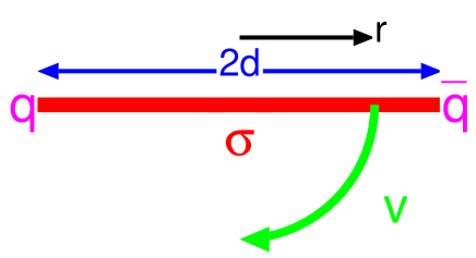
Figure 2.2: Rotating quarks, connected by a string of constant energy density.

A simple explanation of the linear behaviour is provided by the relativistic string model [68, 45]: imagine a rotating string of length $2d$ with a constant energy density per unit length, $\sigma$ (Figure 2.2). If this string spans between (approximately) massless quarks, we might expect those quarks to move at (almost) the speed of light, $c=1$, with respect to the centre of mass. The velocity as a function of the distance from the centre of the string, $r$, in this set-up is given by, $v(r)=r/d$. From this, we calculate the energy stored in the rotating string,

$$m=2\int_{0}^{d}\frac{dr\,\sigma}{\sqrt{1-v^{2}(r)}}=\pi d\sigma,$$ (2.3)

and angular momentum,

$$J=2\int_{0}^{d}\frac{dr\,\sigma\,rv(r)}{\sqrt{1-v^{2}(r)}}=\frac{\pi^{2}d^{2}\sigma}{2}=\frac{1}{2\pi\sigma}m^{2},$$ (2.4)

which results in the relation of Eq. (2.2) between Regge slope, $\alpha^{\prime}$, and string tension, $\sigma$. This crude approximation can of course be improved. For example, one can allow for a rest mass of the quarks. Velocities smaller than $c$ will result in a slight increase of the Regge slope. The assumption that the string energy entirely consists of a longitudinal electric component in the co-rotating frame yields predictions for spin-orbit splittings [42] etc..

For the two Regge trajectories starting with a pseudo-scalar ($\pi$ and $K$), one finds values, $470\,\mbox{MeV}<\sqrt{\sigma}<480$ MeV, while all other numbers scatter between 424 and 437 MeV. The value extracted from the $\rho,a_{2},\ldots$ trajectory, which is the most linear one, is $\sqrt{\sigma}=(429\pm 2)$ MeV.

2.2 Quarkonia

Soon after the discovery of the $J/\psi$ meson in $e^{+}e^{-}$ annihilation, the possibility of a non-relativistic treatment of such states, in analogy to the positronium of electrodynamics, was suggested [11]. Quarkonia, i.e. mesonic states that contain two heavy constituent quarks, either charm or bottom, owe their name to this analogy. Within the quark model, the quark anti-quark system can be characterised by its total spin, ${\mathbf{S}}={\mathbf{S}_{1}}+{\mathbf{S}_{2}}$ ($s=0$ or $s=1$), the relative orbital angular momentum, ${\mathbf{L}}$, and the total spin, ${\mathbf{J}}={\mathbf{L}}+{\mathbf{S}}$. Within the standard spectroscopic notation, $n^{2s+1}l_{J}$, $n$ denotes the radial excitation while $l=0$ is labelled by the letter $S$, $l=1$ by $P$, $l=2$ by $D$ etc.. The parity of a quark anti-quark state is given by, $P=(-1)^{l+1}$, while the charge conjugation operator (if quark and anti-quark share the same flavour) has eigenvalue, $C=(-1)^{l+s}$.

In making the above $J^{PC}$ assignments, we ignore the possibility of the gluonic degrees of freedom contributing to the quantum numbers. This simplification results in certain combinations to be quark model forbidden (or spin-exotic), namely, $J^{PC}=0^{+-},0^{--},1^{-+},2^{+-},3^{-+},\ldots$. Another aspect is that some $J^{PC}$ assignments can be generated in various ways. For instance, ${}^{3}S_{1}$ and ${}^{3}D_{1}$ states both result in $J^{PC}=1^{--}$. As soon as gluons are introduced, the relative angular momentum, ${\mathbf{L}}$, is not conserved anymore and physical vector particles will in general be superpositions of excitations from these two channels: strictly speaking, only the number of nodes of the wave function, $n$, the spin $J$, parity $P$, charge $C$ (in the case of flavour singlet mesons), and the constituent quark content (neglecting annihilation processes and weak decays) represent “good” quantum numbers.

Table 2.3: Classification of charmonium and bottomonium states.

$n^{2s+1}l_{J}$	$J^{PC}$	$c\bar{c}$	$b\bar{b}$
$1^{1}S_{0}$	$0^{-+}$	$\eta_{c}$	$\eta_{b}$
$1^{3}S_{1}$	$1^{--}$	$J/\psi$	$\Upsilon$
$2^{3}S_{1}$	$1^{--}$	$\psi(2S)$	$\Upsilon(2S)$
$1^{1}P_{1}$	$1^{+-}$	$h_{c}$	$h_{b}$
$1^{3}P_{0}$	$0^{++}$	$\chi_{c0}$	$\chi_{b0}$
$1^{3}P_{1}$	$1^{++}$	$\chi_{c1}$	$\chi_{b1}$
$1^{3}P_{2}$	$2^{++}$	$\chi_{c2}$	$\chi_{b2}$

In Table 2.3, we have compiled quantum numbers and names for some members of the $J/\psi$ and $\Upsilon$ families. Little is known experimentally about $B_{c}$ mesons, which are bound states of a $\bar{b}$ and a $c$ quark. For these particles an additional peculiarity has to be considered: charge and total spin are no longer “good” quark model quantum numbers. For $l\geq 1$ this results in mixing between the $J=l$ would-be singlet and would-be triplet states.

Figure 2.3: Energy splittings, $\Delta E$, for charmonia and bottomonia with respect to the $\Upsilon$ and $J/\psi$ triplet $S$ wave states.

In Figure 2.3, all experimentally determined splittings with respect to the $1^{3}S_{1}$ state for the $\Upsilon$ and $J/\psi$ families are depicted. We have restricted ourselves to states, listed in the Review of Particle Properties [82], that are below the $D\overline{D}$ and $B\overline{B}$ thresholds (dashed horizontal lines) for charmonia and bottomonia, respectively, with the exception of the $\Upsilon(4S)$. While the mass of the $J/\psi$ (3.097 GeV) considerably differs from that of the $\Upsilon$ (9.46 GeV), indicating a substantial difference in the quark masses, $m_{b}\approx 3m_{c}$, both $2^{3}S_{1}-1^{3}S_{1}$ splittings agree within 5 % (589 and 563 MeV). We define the spin averaged $\chi$ mass by,

$$m_{\overline{{}^{3}\!P}}=\frac{1}{9}\left(m_{{}^{3}\!P_{0}}+3m_{{}^{3}\!P_{1}}+5m_{{}^{3}\!P_{2}}\right)\approx m_{{}^{1}\!P_{1}}.$$ (2.5)

Again, within a few per cent, the $1\overline{{}^{3}P}-1^{3}S_{1}$ splittings agree (429 MeV vs. 440 MeV). Unfortunately, while the $\eta_{c}$ has been discovered, no pseudo-scalar $b\bar{b}$ ${}^{1}S_{0}$ meson has yet been seen, such that a consistent comparison with respect to spin averaged $S$ state masses,

$$m_{\overline{S}}=\frac{1}{4}\left(m_{{}^{1}\!S_{0}}+3m_{{}^{3}\!S_{1}}\right),$$ (2.6)

is not possible.

While the $2S-1S$ and $1P-1S$ splittings seem to agree within a few per cent, the fine structure splittings between the $P$ states come out to be almost three times as large in the charm case, compared to that for the bottom,

$$\frac{m_{\chi_{b2}}-m_{\chi_{b0}}}{m_{\chi_{c2}}-m_{\chi_{c0}}}=0.38(1)\approx\frac{53\,\mbox{MeV}}{141\,\mbox{MeV}}.$$ (2.7)

This is consistent with the expectation that in the limit of infinite quark mass, fine structure splittings will eventually completely disappear, in analogy to hydrogen-like systems. However, for the ratio between the respective $m_{\chi_{2}}-m_{\chi_{1}}$ splittings one finds a different numerical value, 0.47(2), indicating a more complicated dependence on the inverse quark mass than mere proportionality.

For sufficiently heavy quarks, one might hope that the characteristic time scale associated with the relative movement of the constituent quarks is much larger than that associated with the gluonic (or sea quark) degrees of freedom [11]. In this case the adiabatic (or Born-Oppenheimer) approximation applies and the effect of gluons and sea quarks can be represented by an averaged instantaneous interaction potential between the heavy quark sources. Moreover, the bound state problem will essentially become non-relativistic and the dynamics will, to first approximation, be controlled by the Schrödinger equation,

$$\left[\frac{{\mathbf{p}}^{2}}{2\mu_{R}}+V(r)\right]\psi_{nll_{3}}({\mathbf{r}})=E_{nl}\psi_{nll_{3}}({\mathbf{r}}),$$ (2.8)

with a potential, $V(r)$ ($r=|{\mathbf{r}}|$), or, if spin effects are taken into account, semi-relativistic Pauli-Thomas-like extensions. In the adiabatic approximation quarkonia are the positronium of QCD. However, unlike in QED where the interaction potential can be calculated perturbatively and the spectrum predicted, we are faced with the inverse problem of determining or guessing the interaction potential and the reduced quark mass, $\mu_{R}=m/2$, from the observed spectrum, $E_{nl}$, and decay rates. The latter can be related to properties of the wave function at the origin [16]. If the adiabatic approximation is justified we would expect, to leading order in a semi-relativistic expansion, the same potential to explain $c\bar{c}$ as well as $b\bar{b}$ spectra since QCD interactions are flavour blind. On the other hand it is clear that the adiabatic approximation will at least fail for unstable excitations like the $\Psi(3S)$ or $\Upsilon(4S)$ since decays cannot be accounted for by a one channel Hamiltonian with a real potential.

Table 2.4: The scaling of level splittings, $\Delta E$, inverse length scales, $\langle r^{-1}\rangle$, and the squared velocity, $\langle v^{2}\rangle$, with reduced mass and coupling.

potential	$\Delta E$	$\langle r^{-1}\rangle$	$\langle v^{2}\rangle$
Coulomb, Eq. (2.9)	$e^{2}\mu_{R}$	$e\mu_{R}$	$e^{2}$
logarithmic, Eq. (2.10)	$C$	$C^{-1/2}\mu_{R}^{1/2}r_{0}^{-1}$	$C\mu_{R}^{-1}$
linear, Eq. (2.11)	$\sigma^{2/3}\mu_{R}^{-1/3}$	$\sigma^{1/3}\mu_{R}^{1/3}$	$\sigma^{2/3}\mu_{R}^{-4/3}$

In Appendix A, we derive general properties of the spectrum for power law and logarithmic potentials. The main results for a Coulomb potential,

$$V(r)=-\frac{e}{r},$$ (2.9)

a logarithmic potential,

$$V(r)=C\ln\left(\frac{r}{r_{0}}\right),$$ (2.10)

and a linear potential,

$$V(r)=\sigma\,r,$$ (2.11)

are displayed in Table 2.4.

From the spin-averaged quarkonia spectra it is evident that the underlying potential cannot be purely Coulomb type. Otherwise, the $2S-1S$ splitting would be approximately degenerate with the lowest lying $nP-1S$ splitting and, moreover, $\Upsilon$ splittings would be enhanced with respect to $J/\psi$ splittings by the ratio of the quark masses, $m_{b}/m_{c}\approx 3$. However, a logarithmic potential that would explain the approximate mass independence of spin-averaged splittings is incompatible with tree level perturbation theory, i.e. Eq. (2.9), with $e=(4/3)\alpha_{s}$.

The Cornell potential [12],

$$V(r)=-\frac{e}{r}+\sigma r,$$ (2.12)

contains the perturbative expectation plus an additional linear term. The parameters $e$ and $\sigma$ can be adjusted such that within the range of charm and bottom quark masses, the linear dependence of the Rydberg energy on $\mu_{R}$ is compensated by the $1/\mu_{R}^{1/3}$ behaviour expected from the large distance linear term: within the distance scales relevant for the quarkonium bound state problem, the Cornell potential looks effectively logarithmic. At quark masses larger than $m_{b}$, the Coulomb term will eventually dominate and splittings will diverge in proportion with $\mu_{R}$. Note that the Cornell potential predicts the average velocity, $\langle v^{2}\rangle\propto\Delta E/\mu_{R}$, to saturate at the value $\langle v^{2}\rangle=e^{2}$ for large quark mass while from the approximate equality of bottomonia and charmonia level splittings one would expect $\langle v^{2}_{b}\rangle/\langle v^{2}_{c}\rangle\approx m_{c}/m_{b}$. $\langle v^{2}\rangle$ quantifies the quality of the non-relativistic approximation while the applicability of the adiabatic approximation is more complicated to establish from a QCD perspective.

Before the discovery of the $\Upsilon(2S)$, fits to the spin averaged quarkonia spectra resulted in parameter values [13], $e\approx 0.25$ and $\sqrt{\sigma}\approx 455$ MeV. After inclusion of the $\Upsilon$ states, that probe the potential at smaller distances, values like [16], $e\approx 0.51$ and $\sqrt{\sigma}\approx 412$ MeV, and [17], $e\approx 0.52$ and $\sqrt{\sigma}\approx 427$ MeV, emerged. However, within the region, $0.2\,\mbox{fm}<r<1$ fm, which is effectively probed by spin-averaged quarkonia splittings, the $e\approx 0.25$ parametrisation only marginally differs from the $e\approx 0.5$ parametrisations; the higher value of the Coulomb coefficient is compensated for by a smaller slope, $\sigma$. Interestingly, the slope of the Cornell potential is in qualitative agreement with $\sqrt{\sigma}\approx 430$ MeV, the estimate of the string tension from Regge trajectories of light mesons, discussed in Section 2.1.

While the spin averaged spectrum probes the potential at distances $r>0.2$ fm, fine structure splittings are sensitive towards the Lorentz and spin structure of the interacting force as well as to the functional form of the potential at short distances. We shall discuss this in detail in Section 7.

3 Lattice methods

Lattice QCD was invented by Wilson [1] shortly after QCD emerged as the prime candidate for a consistent theory of strong interactions. The main intention was to define an entirely non-perturbative regularisation scheme for QCD, based on the principle of local gauge invariance. Besides regulating the theory, the lattice lends itself to strong coupling expansion techniques in terms of the inverse QCD coupling,

$$\beta=\frac{2N}{g^{2}}=\frac{2N}{4\pi\alpha_{s}}.$$ (3.1)

Such techniques complement the conventional perturbative weak coupling expansion and have, in particular in the Hamiltonian formulation of lattice QCD [84], stimulated the flux tube model of Ref. [44]. However, so far nobody has managed to analytically relate the strong coupling limit of QCD to weak coupling results. For instance, in $U(1)$ as well as in $SU(N)$ gauge theories one obtains an area law for Wilson loops [Eq. (4.1)], i.e. confinement, in the strong coupling limit. While in $(3+1)$-dimensional $U(1)$ lattice gauge theory the strong coupling regime is separated from a non-confining weak coupling region by a phase transition, in $SU(N)$ one would hope that no such phase transition at finite $\beta$ exists and confinement survives at weak coupling.

Besides offering new analytical insight and techniques, the lattice approach to QCD lends itself to treatment on a computer [85, 86, 2]. To allow for a numerical evaluation of expectation values it is convenient to work in Euclidean space-time in which a path integral measure can be defined. Moreover, the time evolution operator becomes anti-Hermitian which results in $n$-point correlation functions decaying exponentially, rather than exhibiting oscillatory behaviour. Most results that are obtained in Euclidean space can be related to the space-like region of the Minkowski world and can in principle be analytically continued into the time-like region of interest. With results that have been obtained on a discrete set of points with finite precision, however, such a continuation is anything but straight forward. Fortunately, unless one is interested in real time processes like particle scattering, this is in general not required. In particular the mass spectrum remains unaffected by the rotation to imaginary time as long as reflection positivity holds [87], which is the case at least for the lattice actions discussed in this article.

In what follows, the aspects of lattice simulations that are relevant for our discussion are summarised. For a more detailed introduction to Lattice Gauge Theories the reader may consult several books [88, 89, 90, 91] and review articles [92, 86, 93, 94, 95, 96]. The conventions that are adapted throughout the article are detailed in Appendix B.

3.1 What can the lattice do?

The lattice allows for a first principles numerical evaluation of expectation values of a given quantum field theory that is defined by an action $S$ in Euclidean space-time. However, the accessible lattice volumes and resolutions are limited by the available (finite) computer performance and memory.

The obvious strength of lattice methods are hadron mass predictions. Only recently computers have become powerful enough to allow for a determination of the infinite volume light hadron spectrum in the continuum limit in the quenched approximation to QCD within uncertainties of a few per cent [97]. To this accuracy the quenched spectrum has been found to differ from experiment. Some collaborations have started to systematically explore QCD with two flavours of light sea quarks and the first precision results indeed indicate deviations from the quenched approximation in the direction of the experimental values [98]. Even if one is unimpressed by post-dictions of hadron masses that have been known with high precision for decades such simulations allow fundamental standard model parameters to be fixed from low energy input data, like quark masses [99, 100, 101, 102] and the QCD running coupling [103]. Of course, as we shall see, a wealth of other applications of phenomenological importance exists.

Unfortunately, only the lowest radial excitations of a hadronic state are accessible in practice. Lattice predictions are restricted to rather simple systems too. Even the deuteron is beyond the reach of present day super-computers. Therefore, it is desirable to supplement lattice simulations by analytical methods. The computer alone acts as a black box. In order to understand and interprete the output values and to predict their dependence on the input parameters, some modelling is required. Vice versa, the lattice itself is a strong tool to validate models and approximations. Unlike in the “real” world, one can vary the quark masses, $m_{i}$, the number of colours, $N$, the number of flavours, $n_{f}$, the temperature, the spatial volume, the space-time dimension and even the boundary conditions in order to expose models to thorough tests in many situations.

3.2 The method

In a lattice simulation, Euclidean space-time is discretised on a torus with $L_{\sigma}^{3}L_{\tau}$ lattice points or sites, $x=na,n_{i}=0,1,\ldots,L_{\sigma}-1$, $n_{4}=0,1,\ldots,L_{\tau}-1$, separated by the lattice spacing, $a$, that provides an ultra-violet cut-off on the gluon momenta, $q\leq\pi/a$, and regulates the theory. Two adjacent points are connected by an oriented bond or link, $(x,\mu)$. While Dirac quark fields, $q^{i}_{x}$, are represented by $4\times N$ tuples at lattice sites, $x$, gauge fields,

$$U_{x,\mu}={\mathcal{P}}\left[\exp\left(i\int_{x}^{x+a\hat{\mu}}\!dx^{\prime}_{\mu}\,A_{\mu}(x^{\prime})\right)\right]\in SU(N),$$ (3.2)

are “link variables”. ${\mathcal{P}}$ denotes path ordering of the argument and $\hat{\mu}$ is a unit vector pointing into $\mu$ direction. We further define, $U_{x,-\mu}=U^{\dagger}_{x-\hat{\mu},\mu}$. The transformation property of a lattice fermion field under gauge transformations, $\Omega_{x}\in SU(N)$, is [Eq. (B.11)],

$$q(x)\rightarrow\Omega(x)q(x),\quad\bar{q}(x)\rightarrow\bar{q}(x)\Omega^{\dagger}(x).$$ (3.3)

From Eq. (B.10),

$$A_{\mu}\rightarrow A_{\mu}^{\Omega}=\Omega[A_{\mu}-i\partial_{\mu}]\Omega^{\dagger}=-i\Omega D_{\mu}\Omega^{\dagger},$$ (3.4)

one can derive the the transformation property of links,

$$U_{x,\mu}\rightarrow U_{x,\mu}^{\Omega}=\Omega_{x}U_{x,\mu}\Omega_{x+a\hat{\mu}}^{\dagger}.$$ (3.5)

It is easy to see that the trace of a product of links along a closed loop is gauge invariant. Other gauge invariant objects are $N$ gauge transporters whose colour indices are contracted by completely antisymmetric tensors of rank $N$ at a common start and a common end point, a quark and an anti-quark field that are connected by a gauge transporter or a state of $N$ quarks whose colours are transported to a common point, where they are anti-symmetrically contracted. The situation is depicted in Figure 3.1 for $N=3$.

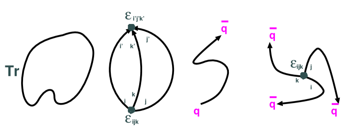
Figure 3.1: Examples of gauge invariant objects. Lines correspond to gauge transporters.

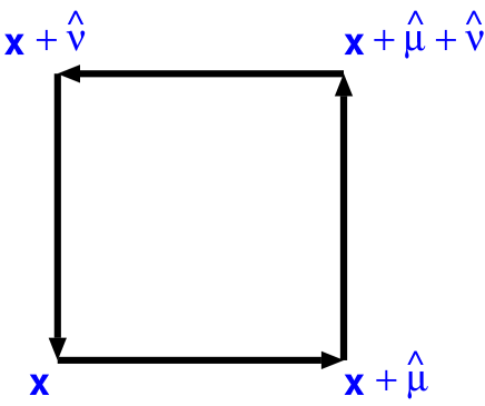
Figure 3.2: The plaquette, $U_{x,\mu\nu}$.

The simplest non-trivial gauge invariant object that can be constructed is the product of four links, enclosing an elementary square,

$$U_{x,\mu\nu}=U_{x,\mu}U_{x+a\hat{\mu},\nu}U^{\dagger}_{x+a\hat{\nu},\mu}U^{\dagger}_{x,\nu},$$ (3.6)

the “plaquette” (Figure 3.2). The plaquette determines the local curvature of the gauge fields within the group manifold, i.e. it is related to the field strength tensor,

$$U_{x,\mu\nu} = \exp\left(ia^{2}{\mathcal{F}}_{x,\mu\nu}\right),$$ (3.7)

$$F^{\alpha\beta}_{\mu\nu}\left(x+\frac{a}{2}\hat{\mu}+\frac{a}{2}\hat{\nu}\right) = \left({\mathcal{F}}^{\alpha\beta}_{x,\mu\nu}-\delta^{\alpha\beta}\mbox{Tr}\,{\mathcal{F}}_{x,\mu\nu}\right)\left[1+{\mathcal{O}}(a^{2})\right],$$ (3.8)

where we denote the normalised trace of an element in a $D$-dimensional representation of the gauge group by $\mbox{Tr}_{D}$ or Tr,

$$\mbox{Tr}\,{\mathbf{1}}_{D}=\mbox{Tr}_{D}{\mathbf{1}}_{D}=\frac{1}{D}\mbox{tr}\,{\mathbf{1}}_{D}=\frac{1}{D}\sum_{i=1}^{D}\delta_{ii}=1.$$ (3.9)

For the fundamental representation above, we have $D=N$. $\alpha,\beta=1,\ldots,N$ label the colours and $F_{\mu\nu}=F_{\mu\nu}^{a}T^{a}$, where the $N\times N$ matrices $T^{a}$ denote the gauge group generators in the fundamental representation. Note that ${\mathcal{F}}_{\mu\mu}=0$ and that ${\mathcal{F}}_{\mu\nu}=-{\mathcal{F}}_{\nu\mu}^{\dagger}$ is anti-hermitian, as a consequence of $U_{\mu\nu}=U^{-1}_{\nu\mu}=U^{\dagger}_{\nu\mu}$.

Discretised lattice actions are formulated in a manifestly gauge-invariant way and should approach the continuum action in the limit, $a\rightarrow 0$. Since the action depends on couplings rather than directly on the lattice spacing, it is not a priori clear if this limit can be realised. We shall discuss the approach to the continuum limit below. For the moment, we remark that from the asymptotic freedom of perturbative QCD we expect $a$ to approach zero as $g\rightarrow 0$, i.e. $\beta\rightarrow\infty$.

The simplest gluonic action is the so-called Wilson action,

$$S_{W}[U]=\beta\sum_{x,\mu>\nu}\left[1-\mbox{Re}\,\mbox{Tr}\left(U_{x,\mu\nu}\right)\right],$$ (3.10)

where Tr denotes the normalised trace of Eq. (3.9). From Eqs. (B.14) and (3.7) it is easy to see that $S_{W}=S_{YM}[1+{\mathcal{O}}(a^{2})]$. The constant term in the action is irrelevant as it cancels from expectation values. The choice of the action is far from unique. For instance an alternative form, suggested by Manton [104], has been used in the glueball studies of Refs. [105, 106]. The action can in principle be systematically improved to approximate the continuum action to a higher order in $a$ [107, 108]. This Symanzik improvement programme has first been applied to Yang-Mills lattice gauge theory by Lüscher and Weisz [109, 110, 111]. In a classical theory, all the coefficients of higher dimensional operators that are added to the plaquette of the Wilson action can easily be determined. However, in the quantum field theory case of interest, the coefficients are subject to radiative corrections, and have to be determined non-perturbatively to fully eliminate the ${\mathcal{O}}(a^{2})$ lattice artefacts of the Wilson action. Although this has not been achieved yet, impressive results on static potentials [112, 113, 114], the glueball spectrum [115, 116, 117] and thermodynamics [118] have recently been obtained with Symanzik improved gluonic actions with coefficients, approximated by a mean field (“tadpole”) estimate [119, 120]. An alternative improved gluonic action that has been used in recent lattice studies [121] is the renormalisation group improved Iwasaki action [122, 123]. The renormalisation group approach towards an improved continuum limit behaviour has been systematised in the work of Hasenfratz and Niedermayer [124] on “perfect” lattice actions. Approximately perfect actions have been constructed for example in Refs. [125, 126, 127].

A naïve discretisation of the Dirac fermionic action of Eq. (B.12) suffers under the fermion doubling problem (cf. Refs. [88, 91]). The simplest way to remove the un-wanted modes is to give them extra mass by adding an irrelevant term, $-a\bar{q}D_{\mu}D_{\mu}q$, to the action. This results in Wilson fermions [128],

$$S_{f}[U,q,\bar{q}]=\sum_{x,y}\bar{q}_{x}M_{xy}(U)q_{y},$$ (3.11)

where

$$M_{xy}=\delta_{xy}-\kappa\sum_{\mu}\left[\left(1-\gamma_{\mu}\right)U_{x,\mu}\delta_{x+\hat{\mu},y}+\left(1+\gamma_{\mu}\right)U^{\dagger}_{x-{\hat{\mu}},\mu}\delta_{x-\hat{\mu},y}\right].$$ (3.12)

One of the disadvantages of this solution is that continuum fermions are only approximated up to ${\mathcal{O}}(a)$ lattice artefacts. Remember that the gauge action was correct up to ${\mathcal{O}}(a^{2})$ errors. The parameter, $\kappa$, is related to the inverse bare quark mass,

$$ma=\frac{1}{2}\left(\frac{1}{\kappa}-\frac{1}{\kappa_{c}}\right),$$ (3.13)

where $\kappa_{c}\geq 1/8$ approaches the free field ($U_{x,\mu}={\mathbf{1}}$) limit, $\kappa_{c}=1/8$, as $\beta\rightarrow\infty$. Note that the quark fields in Eq. (3.11) have been rescaled,

$$q\rightarrow\sqrt{\frac{a^{3}}{2\kappa}}q.$$ (3.14)

Another popular alternative is the Kogut-Susskind action [129] which is correct up to ${\mathcal{O}}(a^{2})$ lattice artefacts. However, it requires four mass degenerate quark flavours. The Sheikoleshlami-Wohlert action [130] is an ${\mathcal{O}}(a)$ Symanzik improved variant of the Wilson fermionic action. The coefficient of the additional term is known non-perturbatively [131]. Other suggestions of Symanzik improved fermionic actions have been put forward for instance by Naik [132] and Eguchi [133]. Domain wall fermions have been suggested [134, 135], in order to realise (approximate) chiral symmetry in the lattice theory. These fermions have received renewed attention since they have been found to fulfil the Ginsparg-Wilson relation [136, 137]. They share this feature with other fermionic actions like the “perfect” action of Ref. [138] and the action derived by use of the overlap formalism [139, 140] in Ref. [141]. However, we are interested in quite the opposite of massless fermions, namely heavy quarks, such that these exciting new developments are of limited interest in the present context.

Expectation values of operators, $O$, are determined by the computation of the path integral,

$$\langle O\rangle=\frac{1}{Z}\int[dU][dq][d\bar{q}]\,O[U]e^{-S[U,q,\bar{q}]}.$$ (3.15)

The normalisation factor, or partition function, $Z$, is such that $\langle{\mathbf{1}}\rangle=1$. The shorthand notation, $q$, represents $\{q^{i}_{x}\}$ and $U$ stands for all gauge fields, $\{U_{x,\mu}\}$. The high-dimensional integral is evaluated by means of a (stochastic) Monte-Carlo method as an average over an ensemble of $n$ representative gauge configurations, ${\mathcal{C}}_{i}=\{U_{x,\mu}^{(i)}\},i=1,\ldots,n$:

$$\langle O\rangle=\frac{1}{n}\sum_{i=1}^{n}O[{\mathcal{C}}_{i}]+\Delta O.$$ (3.16)

Therefore, the result on the expectation value is subject to a statistical error, $\Delta O$, that will decrease like $1/\sqrt{n}$: the more measurements are taken, the more precise the prediction becomes. For this reason one might speak of lattice measurements and lattice experiments, in analogy to “real” experiments. The method represents an exact approach in the sense that the statistical errors can in principle be made arbitrarily small by increasing the sample size, $n$.

3.3 Getting the physics right

In general, the action that is simulated depends on $n_{f}$ quark masses, $m_{i}$, as well as on a bare QCD coupling, $g$. By varying $g$ and $m_{i}$ the lattice spacing, $a(g,m_{i})$, is changed. Lattice QCD is a first principles approach in that no additional parameters are introduced, apart from those that are inherent to QCD, mentioned above. In order to fit these $n_{f}+1$ parameters, $n_{f}+1$ low energy quantities are matched to their experimental values: the lattice spacing, $a(g,m_{i})$, can be obtained for instance by fixing $m_{\rho}$ as determined on the lattice to the experimental value. The lattice parameters that correspond to physical $m_{u}\approx m_{d}$ can then be obtained by adjusting $m_{\pi}/m_{\rho}$; the right $m_{s}$ can be reproduced by adjusting $m_{K}/m_{\rho}$ or $m_{\phi}/m_{\rho}$ to experiment etc..

If the right theory is being simulated all experimental mass ratios should be reproduced in the continuum limit, $a\rightarrow 0$, which will be reached as $g\rightarrow 0$, such that it becomes irrelevant what set of experimental input quantities has been chosen initially. In practice, the available computer speed and memory are finite and simulations are often performed within the quenched approximation, neglecting sea quark effects, or at un-physically heavy quark masses. Therefore, unless controlled extrapolations to the right number of flavours, $n_{f}$, and masses of sea quarks, $m_{i}$, are performed, residual scale uncertainties that depend on the choice of experimental input parameters will survive in the continuum limit. Once the scale and quark masses have been set, everything else becomes a prediction.

Lattice results in general need to be extrapolated to the (continuum) limit, $a\rightarrow 0$, at fixed physical volume. The functional form of this extrapolation is theoretically well understood and under control. This claim is substantiated by the fact that simulations with different lattice discretisations of the continuum QCD action yield compatible results after the continuum extrapolation has been performed. For high energies, an overlap between certain quenched lattice computations and perturbative QCD has been confirmed too [103, 142], excluding the possibility of fixed points of the $\beta$-function at finite values of the coupling, other than $g=0$. After taking the continuum limit, an infinite volume extrapolation should be performed. In most cases, results on hadron masses from quenched evaluations on lattices with spatial extent, $L_{\sigma}a>2$ fm, are virtually indistinguishable from the infinite volume limit within typical statistical errors down to pion masses, $m_{\pi}\approx m_{\rho}/3$. However, for QCD with sea quarks the available information is not yet sufficient for definite conclusions, in particular as one might expect a substantial dependence of the on-set of finite size effects on the sea quark mass(es). The typical lattice spacings used in light hadron spectroscopy cover the region $0.05\,\mbox{fm}<a<0.2$ fm.

The effective infinite volume limit of realistically light pions cannot be realised at a reasonable computational cost, neither in quenched nor in full QCD. Therefore, in practice another extrapolation is required. This extrapolation to the physical light quark mass is theoretically less well under control than those to the continuum and infinite volume limits. The parametrisations used are in general motivated by chiral perturbation theory and the related theoretical uncertainties are the dominant source of error in latest state-of-the-art spectrum calculations [97]. Ideally, the Monte Carlo sample size $n$ is chosen such that the statistical precision is smaller or similar in size than the systematic uncertainty due to the extrapolations involved.

3.4 Mass determinations

In order to extract the ground state mass of a state with quantum numbers $\alpha$, one starts from a connected gauge invariant correlation function,

$$C_{\alpha}(t)=\langle 0|\Psi_{\alpha}^{\dagger}(t)\Psi_{\alpha}(0)|0\rangle-\left|\langle 0|\Psi_{\alpha}|0\rangle\right|^{2},$$ (3.17)

where $|0\rangle$ denotes the vacuum state. $\alpha$ contains the momentum and the $J^{PC}$ quantum numbers of the state of interest as well as the constituent quark content, i.e. isospin, strangeness etc.. In most cases, one is interested in the rest mass. Therefore, $\Psi_{\alpha}$ usually involves a summation over all spatial positions, ${\mathbf{x}}$, within a time slice to project onto spatial momentum, ${\mathbf{p}}={\mathbf{0}}$. Any other lattice momentum can be singled out by taking the corresponding discrete Fourier transform. Due to the translational invariance on the lattice, it is sufficient to project only either source or sink onto the desired momentum state.

In what follows, we will for simplicity assume, $L_{\tau}a\rightarrow\infty$. At finite $L_{\tau}a$ additional contributions arise from the propagation into the negative time direction around the periodically closed temporal boundary. Such effects can easily be taken into account whenever they turn out to be numerically relevant. By inserting a complete set of eigenstates of the Hamiltonian, $|\Phi_{\alpha,n}\rangle$, into Eq. (3.17), one obtains,

$$C_{\alpha}(t)=\sum_{n}|c_{n}(\alpha)|^{2}e^{-E_{n}(\alpha)t}.$$ (3.18)

with

$$c_{n}(\alpha)=\langle\Phi_{\alpha,n}|\Psi_{\alpha}(0)|0\rangle.$$ (3.19)

$E_{n}(\alpha)$ is the energy eigenvalue of the state $|\Phi_{\alpha,n}\rangle$, $e^{-Ht}|\Phi_{\alpha,n}\rangle=e^{-E_{n}(\alpha)t}|\Phi_{\alpha,n}\rangle$, and, $\Psi^{\dagger}_{\alpha}(t)=e^{Ht}\Psi_{\alpha}^{\dagger}(0)e^{-Ht}$. In the limit, $t\rightarrow\infty$, the ground state mass,

$$E_{0}(\alpha)=-\lim_{t\rightarrow\infty}\frac{d}{dt}\ln C_{\alpha}(t),$$ (3.20)

can be extracted. The above formula converges exponentially fast and is, therefore, suitable for numerical studies. In general, $\Psi_{\alpha}$ can be any linear combination of $\Phi_{\alpha,n}$ and its choice is not unique. This observation is exploited in iterative smearing or fuzzing techniques [143, 144, 145, 146, 147, 148, 149] that seek to prepare an initial state with optimised overlap to the level of interest. This will then allow the infinite time limit of Eq. (3.20) to be effectively realised at moderate temporal separations, $t$. In principle, not only a single correlation function but a whole cross-correlation matrix between differently optimised $\Psi$’s can be measured. In doing so, there is the chance that by diagonalising the matrix and employing sophisticated multi-exponential fitting techniques not only the ground state energy can be extracted but also those of the lowest one or two radial excitations [150, 151, 116, 152, 153].

In Eq. (3.18) we have adapted the normalisation convention, $\langle\Phi_{\alpha,m}|\Phi_{\alpha,n}\rangle=\delta_{mn}$, $\sum_{n}|\Phi_{\alpha,n}\rangle\langle\Phi_{\alpha,n}|={\mathbf{1}}$. This results in $0\leq|c_{n}(\alpha)|^{2}\leq 1$ and $\sum_{n}|c_{n}(\alpha)|^{2}=1$. The deviation of $|c_{0}(\alpha)|^{2}$, the ground state overlap, from the optimal value, $|c_{0}(\alpha)|^{2}=1$, determines the quality of the smeared operator, $\Psi_{\alpha}$. It should be noted that if $\Psi_{\alpha}$ contains Dirac spinors, e.g. if it is a pion creation operator, the standard normalisation condition would be, $\langle\Phi_{\pi,m}|\Phi_{\pi,n}\rangle=2m_{\pi,m}\delta_{mn}$, instead. As a consequence, Eq. (3.18) is replaced by,

$$C_{\pi}(t)=\sum_{n}\frac{|c_{\pi,n}|^{2}}{2m_{\pi,n}}e^{-m_{\pi,n}t}.$$ (3.21)

For the manipulations yielding Eq. (3.18) we have assumed the existence of a positive definite self-adjoint Hamiltonian. Lüscher [154] has shown that the Wilson gluonic and fermionic lattice actions fulfil both, reflection positivity [155, 87] with respect to hyperplanes going through lattice sites and through the centre of temporal lattice links (see also Ref. [156]). This feature implies the existence of a positive transfer matrix and the possibility of analytical continuation to Minkowski space-time. Another important consequence of reflection positivity is that the coefficients of the series in Eq. (3.18), are non-negative and that, therefore, the limit of Eq. (3.20) is approached monotonically from above. General properties of the transfer matrix for continuum limit improved actions are discussed in Ref. [157].

3.5 The continuum limit

A continuum limit of the lattice theory can be defined at fixed points associated to phase transitions of second or higher order in the space spanned by the bare couplings of the action. In the vicinity of such a phase transition any correlation length, $\xi/a$, diverges which implies, $a\rightarrow 0$, if we associate $\xi$ to a physical distance or mass, $\xi=1/m$. Moreover, universality sets in, i.e. the behaviour of different correlation lengths is governed by one and the same critical exponent. This results in ratios between two correlation lengths, or masses, to saturate at constant values: the system forgets the lattice spacing, $a$. One refers to this behaviour as “scaling”. In the case of the Wilson gluonic action, the leading order violations of scaling are expected to be proportional to $a^{2}$ while for the Wilson fermionic action, they are only linear in $a$.

The Callan-Symanzik $\beta$-function,

$$\beta(\alpha_{s})=\frac{d\alpha_{s}}{d\ln\mu^{2}}=-\beta_{0}\alpha_{s}^{2}-\beta_{1}\alpha_{s}^{3}-\beta_{2}\alpha_{s}^{4}-\ldots,$$ (3.22)

parameterises the variation of the QCD coupling, $\alpha_{s}=g^{2}/(4\pi)$, with a scale $\mu$. Perturbative QCD tells us, $\beta_{0}>0$ and $\beta_{1}>0$, which implies asymptotic freedom: the limit $\alpha_{s}=0$ is reached with $\mu\rightarrow\infty$, i.e. the continuum limit of lattice QCD, $a\rightarrow 0$, corresponds to $\beta\rightarrow\infty$. Far away from the phase transition, no unique $\beta$-function can be defined; due to the occurrence of power corrections, different masses will in general run differently as a function of the bare coupling. Lattice results seem to imply that in zero temperature $SU(N)$ gauge theory no fixed point other than $\alpha_{s}=0$ exists.

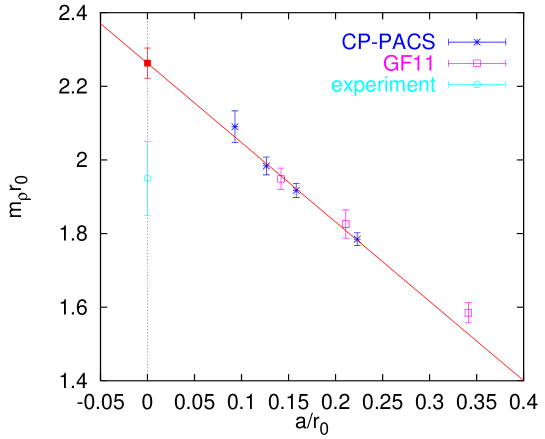
Figure 3.3: The ratio, $m_{\rho}r_{0}$, in quenched QCD, extrapolated to the continuum limit. The $\rho$ masses in lattice units are taken from Refs. [97] (CP-PACS) and [158] (GF11).

While the coefficients $\beta_{0}$ and $\beta_{1}$ within Eq. (3.22) are universal, higher order coefficients depend on the renormalisation scheme. Integrating Eq. (3.22) yields,

$$\mu=\Lambda\exp\left(\int_{\alpha(\Lambda)}^{\alpha(\mu)}\frac{d\alpha}{2\beta(\alpha)}\right),$$ (3.23)

where we define the integration constant, the so-called QCD $\Lambda$-parameter, via the two loop relation,

$$\Lambda=\lim_{\mu\rightarrow\infty}\mu\,\exp\left(-\frac{1}{2\beta_{0}\alpha(\mu)}\right)\left[\beta_{0}\alpha(\mu)\right]^{-\frac{\beta_{1}}{2\beta_{0}}}.$$ (3.24)

In Appendix C, we display results on the coefficients $\beta_{i}$ of Eq. (3.22) for reference and detail how to translate between different schemes.

In QCD with sea quarks, the lattice cut-off, $a$, will not only depend on the coupling but also on the bare quark masses of the Lagrangian. This dependence can be parameterised into quark mass anomalous dimension functions. The continuum limit of a theory with $n_{f}$ different quark masses will be taken along a trajectory on which $n_{f}$ physical mass ratios are kept fixed. In the approximation to QCD with two degenerate light quark masses for instance the physical curve $m_{\pi}/m_{\rho}\approx 2/11$ would serve this purpose.

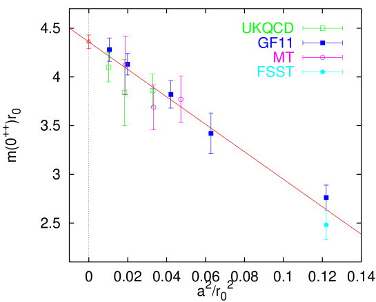
Figure 3.4: The scalar glueball mass in units of $r_{0}$ as a function of $a^{2}$. The glueball masses in lattice units are taken from Refs. [159] (UKQCD), [160] (GF11), [161, 162] (MT) and [163] (FSST).

In Figure 3.3, we show a continuum limit extrapolation of the quantity $m_{\rho}r_{0}$, where $r_{0}$ is a length scale implicitly defined through the static potential [164], $V(r)$,

$$\left.\frac{dV(r)}{dr}\right|_{r=r_{0}}=1.65.$$ (3.25)

From bottomonium phenomenology [164, 29, 30], we can assign the experimental value, $r_{0}^{-1}=(394\pm 20)$ MeV, while $m_{\rho}\approx 770$ MeV. The data on $m_{\rho}$ has been obtained in the quenched approximation to QCD, by use of the Wilson fermionic and gluonic action by the GF11 and CP-PACS collaborations [158, 97]. The corresponding $r_{0}$ values have been obtained from the interpolating formula of the ALPHA collaboration [165] for $5.7\leq\beta\leq 6.57$,

$$a/r_{0}=\exp\left\{-\left[d_{0}+d_{1}(\beta-6)+d_{2}(\beta-6)^{2}+d_{3}(\beta-6)^{3}\right]\right\},$$ (3.26)

with $d_{0}=1.6805,d_{1}=1.7139,d_{2}=-0.8155,d_{3}=0.6667$.

The leading order scaling violations of $m_{\rho}r_{0}$ are expected to be proportional to the lattice spacing, $a$. The data points cover the range, $5.7\leq\beta\leq 6.47$, or, $0.17\,\mbox{fm}\geq a\geq 0.047$ fm. Only the CP-PACS results have been used in the linear fit. In the continuum limit the ratio $m_{\rho}r_{0}$ deviates from the phenomenological estimate by about 15 %, indicating the limitations of the quenched approximation. In Ref. [97] deviations of some quenched ratios between masses of light hadrons from experiment of up to 10 % have been observed.

Due to the substantial slope of the extrapolation, the result obtained on the finest lattice with a resolution of about 4 GeV still deviates by almost 10 % from the continuum limit extrapolated value. This is different from the situation regarding the glueball spectrum where leading order lattice artefacts are proportional to $a^{2}$. In Figure 3.4, we display the continuum limit extrapolation for the lightest quenched glueball mass that has scalar quantum numbers, $J^{PC}=0^{++}$. The $\beta$ range covered in the Figure, $5.7\leq\beta\leq 6.4$, is about the same as that of Figure 3.3. However, within statistical errors, the $\beta=6.4$ results are compatible with the continuum limit and this despite the fact that the scalar glueball behaves rather pathologically [116] in the sense that the slope of this extrapolation is much larger than in any other of the glueball channels. The continuum limit extrapolated mass comes out to be $m(0^{++})=1.485(35)$ GeV or $m(0^{++})=1.720(50)$ GeV, depending on whether the scale is set from the $\rho$-mass or $r_{0}$, respectively; clearly, the dominant source of uncertainty is quenching.

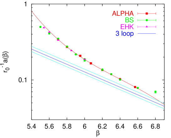
Figure 3.5: The scale, $r_{0}$, in lattice units against the coupling $\beta$. The data are from Refs. [165] (ALPHA), [166, 167] (BS) and [168] (EHK).

Table 3.1: The scale $r_{0}$ in lattice units, obtained from $SU(3)$ gauge theory simulations with Wilson action.

$\beta$	$r_{0}/a$
	[166, 167] (BS)	[168] (EHK)	[165] (ALPHA)	Eq. (3.26)
5.5	2.005(29)
5.54		2.054(13)
5.6	2.439(62)	2.344(8)
5.7	2.863(47)	2.990(24)	2.922(9)	2.930
5.8	3.636(46)		3.673(5)	3.668
5.85		4.103(12)		4.067
5.9	4.601(97)			4.483
5.95			4.808(12)	4.917
6.0	5.328(31)	5.369(9)		5.368
6.07			6.033(17)	6.030
6.2	7.290(34)		7.380(26)	7.360
6.3	8.391(72)			8.493
6.4	9.89(16)		9.74(5)	9.760
6.57			12.38(7)	12.38
6.6	12.73(14)			12.93
6.8	14.36(8)

In Figure 3.5, we plot $r_{0}^{-1}a$ obtained from quenched Wilson action simulations [165, 166, 167, 168] versus the bare coupling, $\beta$. The results are also displayed in Table 3.1. Within the range, $5.5\leq\beta\leq 6.8$, the lattice spacing varies by a factor of about $7$. The interpolating curve for $5.7\leq\beta\leq 6.57$, Eq. (3.26), is included into the plot as well as an estimate obtained by converting the result [103], $\Lambda_{SF}^{(0)}r_{0}=0.294(24)$, into the bare lattice scheme [169] at high energy ($1000\,r_{0}^{-1}$) and running the coupling down to lower scales via Eq. (3.23), using the three loop approximation of the $\beta$-function, Eqs. (3.22), (C.1), (C.2) and (C.4). Taking into account the logarithmic scale, deviations from asymptotic scaling are quite substantial, at least for $\beta\leq 6.4$. One of the reasons for this failure of perturbation theory at energy scales of several GeV are large renormalisations of the lattice action [119], due to contributions from tadpole diagrams [120]. One might hope to partially cancel such contributions by defining an effective coupling [119, 170, 171, 172, 173, 120] from the average plaquette value, measured on the lattice and, indeed, such a procedure somewhat reduces the amount of violations of asymptotic scaling [172, 173].

4 The static QCD potential

We shall introduce the Wegner-Wilson loop and derive its relation to the static potential. Subsequently, expectations on this potential from exact considerations, strong coupling and string arguments as well as perturbation theory and quarkonia phenomenology are presented. Lattice results are then reviewed. Finally, the behaviour of the potential at short distances, the breaking of the hadronic string and aspects of the confinement mechanism are discussed.

4.1 Wilson loops

The Wegner-Wilson loop has originally been introduced by Wegner [174] as an order parameter in $Z_{2}$ gauge theory. It is defined as the trace of the product of gauge variables along a closed oriented contour, $\delta C$, enclosing an area, $C$,

$$W(C)=\mbox{Tr}\left\{{\mathcal{P}}\left[\exp\left(i\int_{\delta C}\!dx_{\mu}\,A_{\mu}(x)\right)\right]\right\}=\mbox{Tr}\left(\prod_{(x,\mu)\in\delta C}U_{x,\mu}\right).$$ (4.1)

While the loop, determined on a gauge configuration, $\{U_{x,\mu}\}$, is in general complex, its expectation value is real, due to charge invariance: in Euclidean space we have, $\langle W(C)\rangle=\langle W^{*}(C)\rangle=\langle W(C)\rangle^{*}=0$. It is straight forward to generalise the above Wilson loop to any non-fundamental representation, $D$, of the gauge field, just by replacing the variables, $U_{x,\mu}$, with the corresponding links, $U_{x,\mu}^{D}$. The arguments below, relating the Wilson loop to the potential energy of static sources go through, independent of the representation according to which the sources transform under local gauge transformations. In what follows, we will denote a Wilson loop, enclosing a rectangular contour with one purely spatial distance, ${\mathbf{r}}$, and one temporal separation, $t$, by $W({\mathbf{r}},t)$. Examples of Wilson loops on a lattice for two different choices of contours, $\delta C$, are displayed in Figure 4.1.

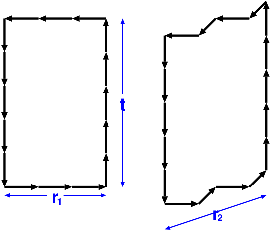
Figure 4.1: Examples of rectangular on- and off-axis Wilson loops with temporal extent, $t=5a$, and spatial extents, $r_{1}=3a$, and, $r_{2}=2\sqrt{2}\,a$, respectively.

In Wilson’s original work [1], the Wilson loop has been related to the potential energy of a pair of static colour sources, by use of transfer matrix arguments. However, it took a few years until Brown and Weisberger attempted to derive the connection between the Wilson loop and the effective potential between heavy, not necessarily static, quarks in a mesonic bound state [175]. Later on mass dependent corrections to the static potential have been derived along similar lines [22, 23]. In Section 6.3, we will discuss these developments in detail. Here, we derive the connection between a Wilson loop and the static potential between colour sources which highlights similarities with the situation in classical electrodynamics and which is close to Wilson’s spirit.

For this purpose we start from the Euclidean Yang-Mills action, Eq. (B.14),

$$S=\frac{1}{4g^{2}}\int\!d^{4}x\,F_{\mu\nu}^{a}F_{\mu\nu}^{a}.$$ (4.2)

The canonically conjugated momentum to the field, $A_{i}^{a}$, is given by the functional derivative,

$$\pi^{a}_{i}=\frac{\delta S}{\delta(\partial_{4}A_{i}^{a})}=\frac{1}{g^{2}}F_{4i}^{a}=-\frac{1}{g}E_{i}^{a}.$$ (4.3)

The anti-symmetry of the field strength tensor implies, $\pi^{a}_{4}=0$. In order to obtain a Hamiltonian formulation of the gauge theory, we fix the temporal gauge, $A_{4}^{a}=0$. In infinite volume, such gauges can always be found. On a toroidal lattice this is possible up to one time slice $t^{\prime}$, which we demand to be outside of the Wilson loop contour, $t^{\prime}>t$.

The canonically conjugated momentum,

$$\pi_{\mu}^{a}=-i\frac{\delta}{\delta A_{\mu}^{a}},$$ (4.4)

now fulfils the usual commutation relations,

$$[A_{j}^{a},\pi_{\mu}^{b}]=i\delta_{j\mu}\delta^{ab},$$ (4.5)

and we can construct the Hamiltonian,

$$H=\int\!d^{3}x\,\left(\pi_{\mu}^{a}\partial_{4}A_{\mu}^{a}-\frac{1}{4g^{2}}F_{\mu\nu}^{a}F_{\mu\nu}^{a}\right)=\frac{1}{2}\int\!d^{3}x\,\left(E_{i}^{a}E_{i}^{a}-B_{i}^{a}B_{i}^{a}\right),$$ (4.6)

that acts onto states, $\Psi[A_{\mu}]$. In Euclidean metric, the magnetic contribution to the total energy is negative.

A gauge transformation, $\Omega$, can for instance be represented as a bundle of $SU(N)$ matrices in some representation $D$, $\Omega_{D}({\mathbf{x}})=e^{i\omega^{a}({\mathbf{x}})T_{D}^{a}}$. We wish to derive the operator representation of the group generators, $T_{R}^{a}$, that acts on the Hilbert space of wave functionals. For this purpose we start from,

$$R(\Omega)\Psi=\left[1+i\int\!d^{3}x\,\omega^{a}({\mathbf{x}})T_{R}^{a}({\mathbf{x}})+\cdots\right]\Psi=\Psi+\delta\Psi.$$ (4.7)

From Eq. (3.4) one easily sees that, $\delta A_{i}=A_{i}^{\Omega}-A_{i}=-(\partial_{i}\omega+i[A_{i},\omega])$. We obtain,

$$\delta\Psi=\int\!d^{3}\!x\,\frac{\delta\Psi}{\delta A_{i}({\mathbf{x}})}\delta A_{i}({\mathbf{x}})=\int\!d^{3}\!x\,\omega({\mathbf{x}})D_{i}\frac{\delta\Psi}{\delta A_{i}({\mathbf{x}})}=-\frac{i}{g}\int\!d^{3}\!x\,\omega^{a}({\mathbf{x}})(D_{i}E_{i})^{a}({\mathbf{x}})\Psi,$$ (4.8)

where we have performed a partial integration and have made use of the equivalence,

$$\frac{\delta}{\delta A_{i}}=-\frac{i}{g}E_{i},$$ (4.9)

of Eqs. (4.3) and (4.4). Hence we obtain the representation,

$$T_{R}^{a}=-\frac{1}{g}(D_{i}E_{i})^{a}:$$ (4.10)

the covariant divergence of the electric field operator is the generator of gauge transformations!

Let us assume that the wave functional is a singlet under gauge transformations, $R(\Omega)\Psi[A_{\mu}]=\Psi[A_{\mu}].$ This implies,

$$(D_{i}E_{i})^{a}\Psi=0,$$ (4.11)

which is Gauß’ law in the absence of sources: $\Psi$ lies in the eigenspace of $D_{i}E_{i}$ that corresponds to the eigenvalue zero. Let us next place an external source in fundamental representation of the colour group at position ${\mathbf{r}}$. In this case, the associated wave functional, $\Psi_{\alpha},\alpha=1,\ldots,N$, transforms in a non-trivial way,

$$[R(\Omega)\Psi]_{\alpha}=\Omega_{\alpha\beta}\Psi_{\beta},$$ (4.12)

This implies,

$$(D_{i}E_{i})^{a}\Psi=-g\delta^{3}({\mathbf{r}})T^{a}\Psi,$$ (4.13)

which again resembles Gauß’ law, this time for a point-like colour charge at position ${\mathbf{r}}$. For non-fundamental representations, $D$, Eq. (4.13) remains valid under the replacement, $T^{a}\rightarrow T^{a}_{D}$.

Let us now place a fundamental source at position ${\mathbf{0}}$ and an anti-source at position ${\mathbf{r}}$. The wave functional, $\Psi_{\mathbf{r}}$, which is an $N\times N$ matrix in colour space will transform according to,

$$\Psi^{\Omega}_{\mathbf{r},\alpha\beta}=\Omega_{\alpha\gamma}({\mathbf{0}})\Omega^{*}_{\beta\delta}({\mathbf{r}})\Psi_{\mathbf{r},\gamma\delta}.$$ (4.14)

One object with the correct transformation property is a gauge transporter (Schwinger line) from ${\mathbf{0}}$ to ${\mathbf{r}}$,

$$\Psi_{\mathbf{r}}=\frac{1}{\sqrt{N}}U^{\dagger}({\mathbf{r}},t)=\frac{1}{\sqrt{N}}{\mathcal{P}}\left[\exp\left(i\int_{\mathbf{0}}^{\mathbf{r}}d{\mathbf{x}}\,{\mathbf{A}}({\mathbf{x}},t)\right)\right],$$ (4.15)

which on the lattice corresponds to the ordered product of link variables along a connection between the two points. Since we are in temporal gauge, $A_{4}(x)=0$, the correlation function between two such lines at time-like separation, $t$, is the Wilson loop,

$$\langle W({\mathbf{r}},t)\rangle=\frac{1}{N}\langle U_{\alpha\beta}({\mathbf{r}},t)U^{\dagger}_{\beta\alpha}({\mathbf{r}},0)\rangle,$$ (4.16)

which, being a gauge invariant object, will give the same result in any gauge. Other choices of $\Psi_{\mathbf{r}}$, e.g. linear combinations of spatial gauge transporters, connecting ${\mathbf{0}}$ with ${\mathbf{r}}$, define generalised (or smeared) Wilson loops, $W_{\Psi}({\mathbf{r}},t)$.

Following the discussion of Section 3.4, we insert a complete set of transfer matrix eigenstates, $|\Phi_{{\mathbf{r}},n}\rangle$, within the sector of the Hilbert space that corresponds to a charge and anti-charge in fundamental representation at distance ${\mathbf{r}}$, and expect the Wilson loop in the limit, $L_{\tau}a\gg t$, to behave like,

$$\langle W_{\Psi}({\mathbf{r}},t)\rangle=\sum_{n}\left|\left\langle\Phi_{\mathbf{r},n}\right|\Psi_{{\mathbf{r}}}\left|0\right\rangle\right|^{2}e^{-E_{n}({\mathbf{r}})t},$$ (4.17)

where the normalisation convention is such that, $\langle\Phi_{n}|\Phi_{n}\rangle=\langle\Psi^{\dagger}\Psi\rangle=1$, and the completeness of eigenstates implies, $\sum_{n}|\langle\Phi_{n}|\Psi|0\rangle|^{2}=1$. Note that no disconnected part has to be subtracted from the correlation function since $\Psi_{\mathbf{r}}$ is distinguished from the vacuum state by its colour indices. $E_{n}({\mathbf{r}})$ denote the energy levels. The ground state contribution, $E_{0}({\mathbf{r}})$, that will dominate in the limit of large $t$ can be identified as the static potential.

The gauge transformation properties of the colour state discussed above, which determine the colour group representation of the static sources and their separation, ${\mathbf{r}}$, do not yet completely determine the state in question: the sources will be connected by an elongated chromo-electric flux tube. This vortex can for instance be in a rotational state with spin $\Lambda\neq 0$ about the inter-source axis. Moreover, under interchange of the ends the state can transform evenly (g) or oddly (u). Finally, in the case of $\Lambda=0$, it can transform symmetrically or anti-symmetrically under reflections with respect to a plane containing the sources. It is possible to single out sectors within a given irreducible representation of the relevant cylindrical symmetry group [176], $D_{\infty h}$, with an adequate choice of $\Psi$. A straight line connection between the sources corresponds to the $D_{\infty h}$ quantum numbers, $\Sigma_{g}^{+}$. Any static potential that is different from the $\Sigma_{g}^{+}$ ground state will be referred to as a “hybrid” potential. Since these potentials are gluonic excitations they can be thought of as being hybrids between pure “glueballs” and a pure static-static state; indeed, high hybrid excitations are unstable and will decay into lower lying potentials via radiation of glueballs. We will address the question of hybrid potentials in detail in Sections 5.2 and 5.3.

4.2 Exact results

We identify the static potential, $V({\mathbf{r}})$, with the ground state energy, $E_{0}({\mathbf{r}})$, of Eq. (4.17) that can be extracted from the Wilson loop of Eq. (4.1) via Eq. (3.20). By exploiting the symmetry of a Wilson loop under an interchange of space and time directions, it can be proven that the static potential cannot rise faster than linearly as a function of the distance $r$ in the limit, $r\rightarrow\infty$ [177]. Moreover, reflection positivity of Euclidean $n$-point functions [155, 87] implies convexity of the static potential [178],

$$V^{\prime\prime}(r)\leq 0.$$ (4.18)

The proof also applies to ground state potentials between sources in non-fundamental representations. However, it does not apply to hybrid potentials since in this case the required creation operator extends into spatial directions orthogonal to the direction of ${\mathbf{r}}$. Due to positivity, the potential is bound from below. Therefore, convexity implies that $V(r)$ is a monotonically rising function of $r$,

$$V^{\prime}(r)\geq 0.$$ (4.19)

In Ref. [179], which in fact preceded Ref. [178], somewhat more strict upper and lower limits on Wilson loops, calculated on a lattice, have been derived: let $a_{\sigma}$ and $a_{\tau}$ be temporal and spatial lattice resolutions. The main result for rectangular Wilson loops in representation $D$ and $d$ space-time dimensions then is,

$$\langle W(a_{\sigma},a_{\tau})\rangle^{rt/(a_{\sigma}a_{\tau})}\leq\langle W(r,t)\rangle\leq(1-c)^{r/a_{\sigma}+t/a_{\tau}-2},$$ (4.20)

with $c=\exp[-4(d-1)D\beta]$. The resulting bounds on $V(r)$ for $r>a_{\sigma}$ read,

$$-\ln(1-c)\leq a_{\tau}V(r)\leq-\frac{r}{a_{\sigma}}\ln\langle W(a_{\sigma},a_{\tau})\rangle;$$ (4.21)

in consistency with Ref. [177], the potential (measured in lattice units, $a_{\tau}$) is bound from above by a linear function of $r$ and it takes positive values everywhere.

4.3 Strong coupling expansions

Expectation values, Eq. (3.15), can be approximated by expanding the exponential of the action, Eq. (3.10), in terms of $\beta$, $\exp(-\beta S)=1-\beta S+\cdots$. This strong coupling expansion is similar to a high temperature expansion in statistical mechanics. When the Wilson action is used each factor, $\beta$, is accompanied by a plaquette and certain diagrammatic rules can be derived [1, 180, 181, 182, 183]. Let us consider a strong coupling expansion of the Wilson loop, Eq. (4.1). Since the integral over a single group element vanishes,

$$\int dU\,U=0,$$ (4.22)

to zeroth order, we have, $\langle W\rangle=0$. To the next order in $\beta$, it becomes possible to cancel the link variables on the contour, $\delta C$, of the Wilson loop by tiling the whole minimal enclosed (lattice) surface, $C$, with plaquettes. Hence, one obtains the expectation value [182, 88, 91],

$$\langle W(C)\rangle=\left\{\begin{array}[]{l}\left[\beta/4\right]^{-\mbox{\scriptsize area}(\delta C)}+\cdots,N=2\\ \left[\beta/2N^{2}\right]^{-\mbox{\scriptsize area}(\delta C)}+\cdots,N>2\end{array}\right.,$$ (4.23)

for $SU(N)$ gauge theory. $\mbox{area}(\delta C)$ denotes the area of the minimal lattice world sheet that is enclosed by the contour $\delta C$.

If we now consider the case of a rectangular Wilson loop that extends $r/a$ lattice points into a spatial and $t/a$ points into the temporal direction, we find the area law,

$$\langle W({\mathbf{r}},t)\rangle=\exp\left[-\sigma_{d}rt\right]+\cdots,$$ (4.24)

with a string tension,

$$\sigma_{d}a^{2}=-d\,\ln\frac{\beta}{18}.$$ (4.25)

The numerical value of the denominator applies to $SU(3)$ gauge theory; the potential is linear with slope, $\sigma_{d}$, and colour sources are confined at strong coupling. $d=(|r_{1}|+|r_{2}|+|r_{3}|)/r\geq 1$ denotes the ratio between lattice and continuum norms and deviates from $d=1$ for source separations, ${\mathbf{r}}$, that are not parallel to a lattice axis. The string tension of Eq. (4.25) depends on $d$ and, therefore, on the lattice direction; $O(3)$ rotational symmetry is broken down to the cubic subgroup $O_{h}$. The extent of violation will eventually be reduced as one increases $\beta$ and considers higher orders of the expansion. Such high order strong coupling expansions have indeed been performed for Wilson loops [184] and glueball masses [185]. Unlike standard perturbation theory, whose convergence is known to be at best asymptotic [186, 187], the strong coupling expansion is analytic around $\beta=0$ [156] and, therefore, has a finite radius of convergence.

Strong coupling $SU(3)$ gauge theory results seem to converge for [88] $\beta<5$. One would have hoped to eventually identify a crossover region of finite extent between the validity regions of the strong and weak coupling expansions [188], or at least a transition point between the leading order strong coupling behaviour, $a^{2}\propto-\ln(\beta/18)$, of Eq. (4.25) and the weak coupling limit, $a^{2}\propto\exp[-2\pi\beta/(3\beta_{0})]$, of Eq. (3.24). However, even after re-summing the strong coupling series in terms of improved expansion parameters and applying sophisticated Padé approximation techniques [189], nowadays such a direct crossover region does not appear to exist, necessitating one to employ Monte Carlo simulation techniques. One reason for the break down of the strong coupling expansion around $\beta\approx 5$ seems to be the roughening transition that is e.g. discussed in Refs. [190, 191]; while at strong coupling the dynamics is confined to the minimal area spanned by a Wilson loop (plus small “bumps” on top of this surface), as the coupling decreases, the colour fields between the sources can penetrate over several lattice sites into the vacuum.

We would like to remark that the area law of Eq. (4.24) is a rather general result for strong coupling expansions in the fundamental representation of compact gauge groups. In particular, it also applies to $U(1)$ gauge theory which we do not expect to confine in the continuum. In fact, based on duality arguments, Banks, Myerson and Kogut [192] have succeeded in proving the existence of a confining phase in the four-dimensional theory and suggested the existence of a phase transition while Guth [193] has proven that, at least in the non-compact formulation of $U(1)$, a Coulomb phase exists. Indeed, in numerical simulations of (compact) $U(1)$ lattice gauge theory two such distinct phases were found [194, 195], a Coulomb phase at weak coupling and a confining phase at strong coupling. The question whether the confinement one finds in $SU(N)$ gauge theories in the strong coupling limit survives the continuum limit, $\beta\rightarrow\infty$, can at present only be answered by means of numerical simulation.

4.4 String picture

The infra-red properties of QCD might be reproduced by effective theories of interacting strings. String models share many aspects with the strong coupling expansion. Originally, the string picture of confinement has been discussed by Kogut and Susskind [84] as the strong coupling limit of the Hamiltonian formulation of lattice QCD. The strong coupling expansion of a Wilson loop can be cast into a sum of weighted random deformations of the minimal area world sheet. This sum can then be interpreted to represent a vibrating string. The physical picture behind such an effective string description is that of the electric flux between two colour sources being squeezed into a thin, effectively one-dimensional, flux tube or Abrikosov-Nielsen-Olesen (ANO) vortex [196, 197, 198, 199]. As a consequence, this yields a constant energy density per unit length and a static potential that is linearly rising as a function of the distance.

One can study the spectrum of such a vibrating string in simple models [200, 190, 47]. Of course, the string action is not a priori known. The simplest possible assumption, employed in the above references, is that the string is described by the Nambu-Goto action [68, 69] in terms of ($d-2$) free bosonic fields associated to the transverse degrees of freedom of the string. In this picture, the static potential is [200, 201] (up to a constant term) given by,

$$V(r)=\sigma r\sqrt{1-\frac{(d-2)\pi}{12\,\sigma\,r^{2}}}=\sigma\,r-\frac{(d-2)\pi}{24\,r}-\frac{(d-2)^{2}\pi^{2}}{1152\,\sigma\,r^{3}}-\cdots,$$ (4.26)

while for a fermionic string [202] one would expect the coefficient of the correction term to the linear behaviour to be only one quarter as big as the Nambu-Goto one above. In the bosonic string picture, excited levels are separated from the ground state by,

$$V_{n}^{2}(r)=V^{2}(r)+(d-2)\pi n\,\sigma=\left[V(r)+\frac{(d-2)\pi n}{2\,r}-\cdots\right]^{2},$$ (4.27)

with $n$ assuming integer values. It is clear from Eq. (4.26) that the string picture at best applies to distances,

$$r\gg r_{c}=\sqrt{\frac{(d-2)\pi}{12\,\sigma}}.$$ (4.28)

In four dimensions one obtains, $r_{c}\approx 0.33$ fm, from the value, $\sqrt{\sigma}\approx 430$ MeV, from the $\rho,a_{2},\ldots$ Regge trajectory.

The expectation of Eq. (4.26) has been very accurately reproduced in numerical simulations of $Z_{2}$ gauge theory in $d=3$ space-time dimensions [203]. In a recent study of $d=4$ $SU(3)$ gauge theory [114] the hybrid potentials have been found to group themselves into various bands that are separated by approximately equi-distant gaps at large $r$. However, up to distances as large as 3 fm these gaps seem to be inconsistent with $\pi/r$, the expectation of Eq. (4.27). These newer data contradict earlier findings in $SU(2)$ gauge theory [146] where good agreement with the Nambu-Goto string picture has been reported, such that we do not regard this issue as finally settled. The consistency of lattice data with Eq. (4.27) at large separations would support the existence of a bosonic string description of confining gauge theories in the very low energy regime [204, 205, 206, 207, 208]. Of course, in $d<26$, the string Lagrangian is not renormalisable but only effective and higher order correction terms like torsion and rigidity will in general have to be added [209].

It is hard to disentangle in $d=4$ the (large distance) $1/r$ term, expected from string vibrations, from the perturbative Coulomb term at short distances. Therefore, three-dimensional investigations (where perturbation theory yields a logarithmic contribution) have been suggested [210]. Another way out is to determine the mass of a closed string, encircling a boundary of the lattice [211] with a spatial extent, $l=L_{\sigma}a$ (a torelon [212]; for details see Appendix D), which is not polluted by a perturbative tail. The bosonic string expectation in this case would be [210],

$$E_{n}(l)=\sigma\,l-\frac{(d-2)\pi}{6\,l}+\cdots.$$ (4.29)

The naïve range of validity of the picture is $l\gg l_{c}=2\,r_{c}\approx 0.66$ fm. The numerical value applies to $d=4$. An investigation of the finite size dependence of the torelon mass in $d=4$ $SU(2)$ gauge theory has been done by Michael and Stephenson [213] who found excellent agreement with the bosonic string picture already for distances, $1\,\mbox{fm}\leq l\leq 2.4$ fm, quite close to $l_{c}$, on the 3 % level. Qualitative agreement has also been reported by Teper [214] from simulations of $SU(2)$, $SU(3)$, $SU(4)$ and $SU(5)$ gauge theories in three dimensions.

The bosonic string picture for $r\gg\beta=aL_{\tau}$ predicts a behaviour similar to Eq. (4.29) for the finite temperature potential, calculated from Polyakov line correlators [215],

$$-\frac{1}{\beta}\ln\langle P^{*}(r)P(0)\rangle=\sigma(\beta)r+\cdots,\quad\sigma(\beta)=\sigma-\frac{(d-2)\pi}{6\beta^{2}}+\cdots.$$ (4.30)

The Polyakov line is defined as [Eq. (D.3)],

$$P({\mathbf{x}})=\mbox{Tr}\,\left\{{\mathcal{T}}\left[\exp\left(i\int_{0}^{aL_{\tau}}\!dx_{4}\,A_{4}(x)\right)\right]\right\}=\mbox{Tr}\,\left(\prod_{x_{4}=0}^{aL_{\tau}}U_{x,4}\right),$$ (4.31)

where ${\mathcal{T}}$ denotes time ordering of the argument. The dependence of the effective string tension on the temperature has recently been checked for rather low $T^{-1}=\beta<1.13\,\beta_{c}\approx 0.85\,\mbox{fm}$ in a study of $SU(3)$ gauge theory [216]. Although the sign of the leading correction term to the zero temperature limit is correct, the difference comes out to be bigger than predicted. It would be interesting to check whether the result will converge towards the string expectation at lower temperatures.

4.5 The potential in perturbation theory

Besides the strong coupling expansion, which is specific to the lattice regularisation, the expectation value of a Wilson loop can be approximated using standard perturbative techniques.

We will discuss the leading order weak coupling result that corresponds to single gluon exchange between the static colour sources which, although we neglect the spin structure, we will call “quarks” for convenience. From the Lagrangian, ${\mathcal{L}}_{YM}=\frac{1}{2g^{2}}\mbox{tr}\,F_{\mu\nu}F_{\mu\nu}$, one can easily derive the propagator of a gluon with four-momentum, $q$,

$$G^{ab}_{\mu\nu}(q)=g^{2}\frac{\delta^{ab}\delta_{\mu\nu}}{q^{2}},$$ (4.32)

where $\mu,\nu$ are Lorentz indices and $a,b=1,\ldots N_{A}=N^{2}-1$ label the colour generators. The same calculation can be done, starting from a lattice discretised action. The Wilson action, Eq. (3.10), yields the result of Eq. (4.32), up to the replacement,

$$q_{\mu}\rightarrow\hat{q}_{\mu}=\frac{2}{a}\sin\left(\frac{aq_{\mu}}{2}\right).$$ (4.33)

Other lattice actions yield slightly different results but they all approach Eq. (4.32) in the continuum limit, $a\rightarrow 0$. Up to order $\alpha_{s}^{2}$, the momentum space potential can be obtained from the on-shell static quark anti-quark scattering amplitude: the gluon interacts with two static external currents pointing into the positive and negative time directions, $A^{a}_{\mu,\alpha\beta}=\delta_{\mu,4}T^{a}_{\alpha,\beta}$ and $A_{\nu,\alpha\beta}^{\prime b}=-\delta_{\nu,4}T^{b}_{\gamma,\delta}$. Hence, we obtain the tree level interaction kernel,

$$K_{\alpha\beta\gamma\delta}(q)=-\frac{g^{2}}{q^{2}}T^{a}_{\alpha\beta}T^{a}_{\gamma\delta}.$$ (4.34)

For sources in the fundamental representation, the Greek indices run from $1$ to $N$ and the quark anti-quark state can be decomposed into two irreducible representations of $SU(N)$,

$${\mathbf{N}}\otimes{\mathbf{N}^{*}}={\mathbf{1}}\oplus{\mathbf{N}_{A}}.$$ (4.35)

We can now either start from a singlet or an octet initial $\Phi_{\beta\gamma}=Q_{\beta}Q^{*}_{\gamma}$ state,

$$\Phi^{\mathbf{1}}_{\beta\gamma} = \delta_{\beta\gamma},$$ (4.36)

$$\Phi^{\mathbf{N}_{A}}_{\beta\gamma} = \Phi_{\beta\gamma}-\frac{1}{N}\delta_{\beta\gamma},$$ (4.37)

where the normalisation is such that $\Phi^{i}_{\alpha\beta}\Phi^{j}_{\beta\alpha}=\delta^{ij}$. A contraction with the group generators of Eq. (4.34) yields,

$$\Phi^{\mathbf{1}}_{\beta\gamma}T_{\alpha\beta}^{a}T_{\gamma\delta}^{a} = C_{F}\Phi^{\mathbf{1}}_{\alpha\delta},$$ (4.38)

$$\Phi^{\mathbf{N}_{A}}_{\beta\gamma}T_{\alpha\beta}^{a}T_{\gamma\delta}^{a} = -\frac{1}{2N}\Phi^{\mathbf{N}_{A}}_{\alpha\delta},$$ (4.39)

where $C_{F}=N_{A}/(2N)$ is the quadratic Casimir charge of the fundamental representation.

We end up with the potentials in momentum space,

$$V_{s}(q)=-C_{F}g^{2}\frac{1}{q^{2}},\quad V_{o}(q)=\frac{g^{2}}{2N}\frac{1}{q^{2}}=-\frac{1}{N_{A}}V_{s}(q),$$ (4.40)

governing interactions between fundamental charges coupled to a singlet and to an octet, respectively: the force in the singlet channel is attractive while that in the octet channel is repulsive and smaller in size.

How are these potentials related to the static position space inter-quark potential, defined non-perturbatively through the Wilson loop,

$$V({\mathbf{r}})=-\lim_{t\rightarrow\infty}\frac{d}{dt}\ln\langle W({\mathbf{r}},t)\rangle?$$ (4.41)

The quark anti-quark state creation operator, $\Psi_{\mathbf{r}}$, within the Wilson loop contains a gauge transporter and couples to the gluonic degrees of freedom. Thus, in general, it will have overlap with both, $QQ^{*}$ singlet and octet channels. Since the singlet channel is energetically preferred, $V_{s}<V_{o}$, we might expect the static potential to correspond to the singlet potential.

To lowest order in perturbation theory, the Wilson loop is given by the Gaussian integral,

$$\langle W({\mathbf{r}},t)\rangle=\exp\left\{-\frac{1}{2}\int\!d^{4}x\,d^{4}yJ^{a}_{\mu}(x)G^{ab}_{\mu\nu}(x-y)J^{b}_{\nu}(y)\right\},$$ (4.42)

where $J_{\mu}^{a}=\pm T^{a}$ if $(x,\mu)\in\delta C$ and $J_{\mu}^{a}=0$, elsewhere. Eq. (4.42) implies for $t\gg r$,

$$\langle W({\mathbf{r}},t)\rangle=\exp\left(C_{F}g^{2}t\int_{-t/2}^{t/2}\!dt^{\prime}\ [G({\mathbf{r}},t^{\prime})-G({\mathbf{0}},t^{\prime})]\right).$$ (4.43)

We have omitted gluon exchanges between the spatial closures of the Wilson loop from the above formula. Up to order $\alpha_{s}^{3}$ (two loops), such contributions result in terms whose exponents are proportional to $r$ and $r/t$ and, therefore, do not affect the potential of Eq. (4.41). $G^{ab}_{\mu\nu}(x)$, the Fourier transform of $G^{ab}_{\mu\nu}(q)$, contains the function,

$$G(x)=\int\frac{d^{4}q}{(2\pi)^{4}}\frac{e^{iqx}}{q^{2}},\quad\int_{-\infty}^{\infty}\!dx_{4}\,G(x)=\frac{1}{4\pi}\frac{1}{r}.$$ (4.44)

After performing the $t$-integration, we obtain,

$$V({\mathbf{r}},\mu)=-C_{F}\frac{\alpha_{s}}{r}+V_{\mbox{\scriptsize self}}(\mu),$$ (4.45)

where $\alpha_{s}=g^{2}/(4\pi)$. The piece,

$$V_{\mbox{\scriptsize self}}(\mu)=C_{F}g^{2}\int_{q\leq\mu}\frac{d^{3}q}{(2\pi)^{3}}\frac{1}{q^{2}}=C_{F}\alpha_{s}\frac{2}{\pi}\mu,$$ (4.46)

that linearly diverges with the ultra-violet cut-off, $\mu$, results from self-interactions of the static (infinitely heavy) sources. Beyond tree level, $g^{2}$ will depend on $q$, such that $\alpha_{s}$ in momentum space has to be replaced by $\alpha_{s}(q^{*})$ with some effective $q^{*}(\mu)$. We find,

$$V(q)=V_{s}(q),$$ (4.47)

where

$$V({\mathbf{q}},0)=\int\!d^{3}r\,e^{i{\mathbf{q}}\cdot{\mathbf{r}}}\hat{V}({\mathbf{r}}),\quad\hat{V}({\mathbf{r}})=V({\mathbf{r}},\mu)-V_{\mbox{\scriptsize self}}(\mu).$$ (4.48)

This self-energy problem is well known on the lattice and has recently received attention in continuum QCD, in the context of renormalon ambiguities in quark mass definitions [217, 218].

At order $\alpha_{s}^{4}$ a class of diagrams appears in a perturbative calculation of the Wilson loop that results in contributions to the static potential that diverge logarithmically with the interaction time [219]. In Ref. [220], within the framework of effective field theories, this effect has been related to ultra-soft gluons due to which an extra scale, $V_{o}-V_{s}$, is generated. Moreover, a systematic procedure has been suggested to isolate and subtract such terms to obtain a finite interaction potential between heavy quarks. However, one would wish to understand and regulate such contributions not only for heavy quarks but also in the static case. At present it is not clear whether the interaction potential within a heavy quark bound state whose effective Hamiltonian contains a kinetic term will, in the limit of infinite quark masses, approach the static potential that is defined through the Wilson loop. Hence, one should carefully distinguish between the static and heavy quark potentials. We shall discuss a physically motivated reason for the breakdown of standard high order perturbative calculations of the Wilson loop in Section 4.8. In our opinion the presence of a low energy scale, which we shall identify with the gap between ground state potential and hybrid excitations, results in problems within perturbation theory in the limit of large $t$.

That something in the position space derivation of the perturbative potential might be problematic is reflected in Eq. (4.43) that contains an integration over the interaction time. We know for instance from the spectral decomposition of Section 3.4 that for any fixed distance $r$, Wilson loops will decay exponentially in the limit of large $t$. However, the tree level propagator in position space is proportional to, $(r^{2}+t^{2})^{-1}$, i.e. asymptotically decays with $t^{-2}$ only. We notice that the integral receives significant contributions from the region of large $t$ as demonstrated by the finite $t\gg r$ tree level result,

$$-\ln\langle W(r,t)\rangle=-\frac{C_{F}\alpha_{s}}{r}t\frac{2}{\pi}\left\{\arctan\frac{t}{r}-\frac{r^{2}}{2t}\left[\ln\left(1+\frac{t^{2}}{r^{2}}\right)\right]\right\}+(r+t)V_{\mbox{\scriptsize self}}.$$ (4.49)

Ignoring this problem for the moment, one finds the weak coupling equality, Eq. (4.47), to hold up to two loops (order $\alpha_{s}^{3}$) in perturbation theory. Some of the hybrid potentials of Section 5.2 that can be extracted from generalised Wilson loops, $\langle W_{\Psi}\rangle$, in which the wave function, $\Psi$, transforms non-trivially under the cylindrical rotation group $D_{\infty h}$, however, receive leading order octet contributions. This is because the creation operator, $\Psi$, explicitly couples to the gluonic background.

The tree level lattice potential can easily be obtained by replacing $q_{\mu}$ by $\hat{q}_{\mu}$ and (in the case of finite lattice volumes) the integrals by discrete sums over lattice momenta,

$$q_{i}=\frac{2\pi}{L_{\sigma}}\,\frac{n_{i}}{a},\quad n_{i}=-\frac{L_{\sigma}}{2}+1,\ldots,\frac{L_{\sigma}}{2}.$$ (4.50)

The lattice potential reads,

$$V({\mathbf{r}})=V_{\mbox{\scriptsize self}}(a)-C_{F}\alpha_{s}\left[\frac{1}{{\mathbf{r}}}\right],$$ (4.51)

where

$$\left[\frac{1}{{\mathbf{r}}}\right]=\frac{4\pi}{L_{\sigma}^{3}a^{3}}\sum_{{\mathbf{q}}\neq{\mathbf{0}}}\frac{e^{i{\mathbf{q}R}}}{\sum_{i}\hat{q}_{i}\hat{q}_{i}},$$ (4.52)

and $V_{\mbox{\scriptsize self}}(a)=C_{F}\alpha_{s}\left[1/{\mathbf{0}}\right]$. We have neglected the zero mode contribution that is suppressed by the inverse volume, $(aL_{\sigma})^{-3}$. In the continuum limit, $[1/{\mathbf{r}}]$ approaches $1/r$ up to quadratic lattice artefacts whose coefficients depend on the direction of ${\mathbf{r}}$ while $V_{\mbox{\scriptsize self}}(a)$ with $n_{f}$ flavours of Wilson fermions diverges like [221, 222],

$$V_{\mbox{\scriptsize self}}(a)=C_{F}\alpha_{s}a^{-1}\left[3.1759115\ldots+\left(16.728\ldots-0.423\ldots n_{f}\right)\alpha_{s}\right].$$ (4.53)

The numerical values apply to the limit, $L_{\sigma}\rightarrow\infty$ and, in the case of the one loop coefficient, $N=3$. Note that under the substitution, $\mu\approx 1.5879557\,\pi/a$, the tree level term of Eq. (4.53) is identical to Eq. (4.46). A one loop computation of on-axis lattice Wilson loops in pure gauge theories can be found in Ref. [221]. The tree level form, Eq. (4.51), is often employed to parameterise lattice artefacts.

Besides defining the static potential from Wilson loops, on a volume with temporal extent, $\beta=aL_{\tau}$, and periodic boundary conditions it can be extracted from Polyakov line correlators,

$$V(r)=-\lim_{\beta\rightarrow\infty}\frac{d}{d\beta}\langle P^{*}(r)P(0)\rangle:$$ (4.54)

at any given time the pair of Polyakov lines has the gauge transformation properties of a static quark anti-quark pair and, thus, the ground state is the same as that of a Wilson loop. In the Polyakov line correlator, no projection is made onto the $\Sigma_{g}^{+}$ ground state of the flux tube. Therefore, one might expect [223],

$$\langle P^{*}(r)P(0)\rangle\approx\frac{1}{N^{2}}\left[e^{-\beta V_{s}({\mathbf{r}})}+N_{A}e^{-\beta V_{o}({\mathbf{r}})}\right],$$ (4.55)

where the “octet” potential, $V_{o}$, can be thought to be related to hybrid excitations of the inter-quark string. At small $\beta$ (high temperature) the exponentials can be expanded and the term proportional to $g^{2}$ vanishes due to $V_{s}=-N_{A}V_{o}$: the leading order $r$ dependent contribution to the correlation function requires two gluons to be exchanged,

$$\langle P^{*}(r)P(0)\rangle=\left(1+\frac{N_{A}}{8N^{2}}\alpha_{s}^{2}\frac{\beta^{2}}{r^{2}}\right)e^{-\beta V_{\mbox{\tiny self}}}.$$ (4.56)

The above result can also be produced by a direct perturbative evaluation of the Polyakov line correlator in position space: the correlation function contains two disjoint colour traces, therefore, single gluon exchanges only contribute to the self-energy. The colour factor that accompanies two gluon exchanges is, $\frac{1}{N}\mbox{tr}\,(T^{a}T^{b})\delta^{ac}\delta^{bd}\frac{1}{N}\mbox{tr}\,(T^{c}T^{d})=\frac{N_{A}}{4N^{2}}$. Hence, we indeed reproduce Eq. (4.56). By assuming the singlet channel ($V_{s}<V_{o}$) to dominate Eq. (4.55) in the asymptotic limit of large $\beta$ one obtains the result of Eq. (4.45), i.e. the same potential as from Wilson loops. However, if we insist on perturbation theory to hold for the correlation function itself at large $\beta$, i.e. at low temperature, a misleading (and divergent) result is obtained. We have demonstrated that extra information how to treat the limit $\beta\rightarrow\infty$ has to be provided to obtain the correct zero temperature tree level potential from Polyakov line correlation functions. We take this as an indication that in three loop calculations of the Wilson loop the $t\rightarrow\infty$ limit should be performed with caution too.

4.6 Potential models

Several parametrisations of the QCD potential have been suggested in the past, either QCD inspired or purely phenomenological. One should keep in mind that one would not necessarily expect a potential that reproduces the observed quarkonia levels to coincide with the static potential calculated from QCD, due to the approximations involved, namely the adiabatic and non-relativistic approximations.

A purely phenomenological logarithmic potential, $V(r)=C\ln(r/r_{0})$, has been suggested as an easy way to produce identical spin-averaged charmonia and bottomonia level splittings [224]. This idea has been incorporated into the Martin potential [18, 19], $V(r)=C+(r/r_{0})^{\alpha}$, with $\alpha\approx 0.1$. Potentials that have QCD-like behaviour built in at small distances have been suggested for instance in Refs. [12, 15, 20]. We have already discussed the prototype Cornell potential [12], $\hat{V}(r)=-e/r+\sigma r$, that interpolates between perturbative one gluon exchange for small distances and a linear confining behaviour for large distances. Another elegant interpolation between the two domains, containing the one loop running of the QCD coupling,

$$\alpha_{V}(q)=\frac{1}{\beta_{0}t_{V}},\quad t_{V}=\ln\left(\frac{q^{2}}{\Lambda_{V}^{2}}\right),$$ (4.57)

has been suggested by Richardson [15]: in momentum space, $t_{V}$ is substituted by, $t_{V}^{\prime}=\ln(1+q^{2}/\Lambda_{V}^{2})$, which does not affect the perturbative ultra-violet domain since $t_{V}^{\prime}\rightarrow t_{V}$ as $q^{2}\rightarrow\infty$. However, the Landau pole at $q^{2}=\Lambda_{V}^{2}$ is regulated and the low energy behaviour of the resulting potential,

$$V(r)=-\frac{4\pi C_{F}}{\beta_{0}}\int\frac{d^{3}q}{(2\pi)^{3}}\frac{e^{i{\mathbf{q}}{\mathbf{r}}}}{q^{2}\ln(1+q^{2}/\Lambda_{V}^{2})},$$ (4.58)

is given by,

$$V(r) \rightarrow \sigma r\quad(r\rightarrow\infty),$$ (4.59)

$$\sigma = \frac{C_{F}}{2\beta_{0}}\Lambda_{V}^{2},$$ (4.60)

i.e. the ansatz connects the QCD scale parameter, $\Lambda_{V}$ to the string tension, $\sigma$. We have neglected an infinite additional constant from Eq. (4.59) that can be eliminated by adding an appropriate counter term to the integrand of Eq. (4.58).

From Eq. (4.60) and the relation,

$$\Lambda_{V}=\Lambda_{\overline{MS}}e^{a_{1}/(2\beta_{0})},$$ (4.61)

with [225, 219],

$$a_{1}=\left(\frac{31}{3}-\frac{10}{9}n_{f}\right)\frac{1}{4\pi},$$ (4.62)

we find $\Lambda_{\overline{MS}}/\sqrt{\sigma}\approx 0.71639$ for $n_{f}=0$ or $\Lambda_{\overline{MS}}/\sqrt{\sigma}\approx 0.70253(0.70048)$ for $n_{f}=3(4)$, respectively. This has to be compared to the value, $\Lambda_{\overline{MS}}/\sqrt{\sigma}=0.52\pm 0.05$, determined by lattice simulations [103, 166] for $n_{f}=0$. Experimental results from $e^{+}e^{-}$ scattering experiments at LEP and SLAC indicate somewhat bigger ratios [82], $\Lambda_{\overline{MS}}^{(4)}/\sqrt{\sigma}=0.88(12)$ MeV, for $n_{f}=4$, where we have assumed, $\sqrt{\sigma}=(430\pm 20)$ MeV: while the Richardson potential overestimates the $\Lambda$-parameter in the quenched case it might approximate the experimental $n_{f}=3$ situation quite well. However, this coincidence is rather accidental.

Many so-called QCD potentials have been suggested that incorporate two loop perturbation theory at short distances, with varying interpolation prescriptions to different assumptions on the large distance behaviour. The most popular potential within this class is probably the Buchmüller-Tye parametrisation [20] that, like the Richardson potential, is formulated in momentum space. For collections of various parametrisations, we refer to Refs. [226, 227]. While phenomenological potentials like a logarithmic as well as the Martin potential are ruled out at large and intermediate distances by lattice data and at short distances by pQCD, such parametrisations may still serve to explore the sensitivity of the heavy quark spectrum towards QCD.

Basically, all potentials that yield a correct description for the spin-averaged quarkonia spectra are only slight variations around the Cornell potential in the relevant region, $0.2\,\mbox{fm}<r<1$ fm. Unfortunately, the top quark is too heavy to form stable hadronic states and basically only the production rate of $t\bar{t}$ in $e^{+}e^{-}$ or $\mu^{+}\mu^{-}$ collisions as a function of the energy will directly depend on the potential at very short distances. Decay rates and fine structure splittings of quarkonia in principle can probe the potential at short distances too and predictions of these quantities indeed depend very sensitively on the underlying ansatz [228]. As we will see in Sections 6 and 7.2, the predictive power of quarkonium physics on the short range potential is reduced by theoretical uncertainties in the matching of an effective field theory to QCD. A big part of the (multiplicative) uncertainty in the fine structure, however, cancels from ratios of such splittings.

4.7 Lattice results

The static QCD potential has been determined to high accuracy in quenched lattice studies with Wilson [229, 230, 231, 232, 233, 234, 235, 215, 236, 237, 238, 146, 239, 240, 147, 241, 173, 166, 242, 168] as well as various improved lattice actions [243, 121, 113, 118, 114] in $SU(2)$ and $SU(3)$ gauge theories. Results for QCD with sea quarks have been obtained in Refs. [244, 245, 246, 167, 247, 248, 249]. After discussing the methods most commonly used we will present results on the potential in QCD, without and with sea quarks.

4.7.1 Evaluation method

The relative statistical errors of Wilson loop expectation values turn out to increase exponentially fast with the Euclidean time extent, $t$, of the loop. Therefore, after some pioneering studies [229, 230, 232, 233, 234], replacement of the straight spatial connection within the Wilson loop by operators with improved overlap to the physical ground state turned out to be essential for a reliable determination of the potential at large distances from data at moderate $t$ separations. For this purpose, in Refs. [231, 235, 236], linear combinations of certain spatial paths connecting quark and anti-quark were employed. Subsequently, iterative smearing techniques [143, 144, 146, 147] turned out to be extremely successful in optimising the ground state overlap.

Among all algorithmic and technical tricks employed in lattice simulations smearing is certainly the most important one. The underlying concept somewhat resembles that of cooling techniques that are applied to extract classical properties of quantum field configurations [250] with the difference that, since smearing is a purely spatial procedure, the spectrum of the theory remains unaffected: fat links are iteratively constructed by replacing a given link by the sum of itself and the neighbouring six (in $d=3+1$ dimensions) spatial staples with some weight parameter, $\alpha>0$,

$$U_{x,i}\rightarrow P_{SU(N)}\left(U_{x,i}+\alpha\sum_{j\neq i}U_{x,j}U_{x+\hat{\jmath},i}U^{\dagger}_{x+\hat{\imath},j}\right).$$ (4.63)

$P_{SU(N)}$ denotes a projection operator, back onto the $SU(N)$ manifold. One possible definition is [147], $U=P_{SU(N)}(A)\in SU(N)$, $\mbox{Re}\,\mbox{tr}\,UA^{\dagger}=\max$. The procedure, Eq. (4.63), can be iterated several times over the whole lattice. The number of iterations and $\alpha$ represent free parameters which can be varied to optimise the overlap of an operator, constructed from the fat links, with the physical ground state in question. Several variations of the algorithm exist. For example, all links within a given timeslice can be replaced at once or several subgroups can be replaced, subsequently. Blocking or fuzzing algorithms can be used, in which a fat link of smearing level $n$ extends over more lattice sites than the previous links of level $n-1$. Smearing and fuzzing can be combined etc.. All smearing and fuzzing methods have in common that the expectation value of a plaquette built from fat spatial links is increased during the iterations, similar to cooling, which means that the contribution to the gauge action from spatial links is reduced: the movement of the magnetic field through colour space under a change of the spatial position is minimised. Operators, built from such fat links, are likely to effectively decouple from excitations since the ground state wave function is always the smoothest wave function within any given channel. Smearing or fuzzing methods can be combined with variational minimisation techniques when determining a correlation matrix between a set of different operators [146], to achieve further improvement.

The potential is finally extracted from expectation values of smeared Wilson loops, $W({\mathbf{r}},t)$, where the spatial transporters are constructed from fat links,

$$V({\mathbf{r}}) = \lim_{t\rightarrow\infty}V({\mathbf{r}},t),$$ (4.64)

$$V({\mathbf{r}},t) = -\frac{d}{dt}\ln\langle W({\mathbf{r}},t)\rangle\approx a_{\tau}^{-1}\ln\frac{\langle W({\mathbf{r}},t)\rangle}{\langle W({\mathbf{r}},t+a_{\tau})\rangle}.$$ (4.65)

$a_{\tau}$ denotes the temporal lattice spacing. On the lattice, the limit of large temporal separation is approximated by a single- or multi-exponential fit to Wilson loops for a range, $t>t_{\min}({\mathbf{r}})$. Positivity of the transfer matrix implies that $V({\mathbf{r}},t)$ converges towards the asymptotic value, $V({\mathbf{r}})$, monotonically from above, a feature that is essential for the reliable detection of saturation of effective masses, $V({\mathbf{r}},t)$, into a plateau. In general, within given statistics, $t_{\min}({\mathbf{r}})$ will depend on the distance, ${\mathbf{r}}$. Within the typical window of lattice spacings, 0.2 fm $\geq a\geq 0.05$ fm, in pure gauge theories and standard smearing and simulation techniques, this dependence happens to be weak. However, this does not necessarily have to be so but depends very much on the interplay between the dynamics of the underlying theory, smearing methods and statistical errors.

In order to illustrate the importance of a careful analysis of the $t$ dependence of the lattice data we consider the case of an unsmeared on-axis Wilson loop on an isotropic lattice, $\langle W(r,t)\rangle=\langle W(t,r)\rangle$. For $t\gg r$, we expect $\langle W(r,t)\rangle\propto e^{-V(r)t}$. The symmetry under interchange of $r$ and $t$ implies, $\langle W(r,t)\rangle\propto e^{-V(t)r}$ for $r\gg t$. This means,

$$V(r,t)=\sigma_{\mbox{\scriptsize eff}}(t)r,\quad\sigma_{\mbox{\scriptsize eff}}(t)=V^{\prime}(t)$$ (4.66)

Thus, approximating $V(r)$ by an effective potential, $V(r,t_{\min})$, with an $r$-independent value of $t_{\min}$ automatically implies a linear rise [242, 251] within the region, $r\gg t_{\min}$, for any potential with non-vanishing derivative. This illustrates the importance of separately investigating the approach to the plateau for each distance. Let us examine closely the situation for the Cornell potential, $V(r)=V_{\mbox{\scriptsize self}}+\sigma r-e/r$. In this case, taking one and the same $t$-value for all separations we find,

$$\sigma_{\mbox{\scriptsize eff}}(t)=\sigma+\frac{e}{t^{2}};$$ (4.67)

even a pure Coulomb potential, $\sigma=0$, implies a non-vanishing $\sigma_{\mbox{\scriptsize eff}}$ at finite $t\ll r$. Of course, the symmetry of the Wilson loop under interchange of $r$ and $t$ also implies that no plateau in $V(r,t)$ can be found, unless $t\gg r$. For smeared Wilson loops, one would still expect a similar $1/t^{2}$ approach (with a different coefficient) of $\sigma_{\mbox{\scriptsize eff}}$ towards the asymptotic limit, while effective masses, $V(r,t)$, will approach $V(r)$ exponentially fast at any $r$.

4.7.2 The quenched potential

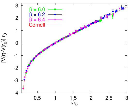
Figure 4.2: The quenched Wilson action $SU(3)$ potential, normalised to $V(r_{0})=0$.

In Figure 4.2, we display the quenched potential, obtained at three different $\beta$ values in units of $r_{0}\approx 0.5$ fm from the data of Refs. [173, 29]. The lattice spacings, determined from $r_{0}$, correspond to $a\approx 0.094$ fm, 0.069 fm and 0.051 fm, respectively. The curve represents the Cornell parametrisation with $e=0.295$. At small distances the data points lie somewhat above the curve, indicating a weakening of the effective coupling and, therefore, asymptotic freedom. We will discuss this observation later. All data points for $r>4a$ collapse onto a universal curve, indicating that for $\beta\geq 6.0$ the scaling region is effectively reached for the static potential. Moreover, continuum rotational symmetry is restored: in addition to on-axis separations, many off-axis distances of the sources have been realised and the corresponding data points are well parameterised by the Cornell fit for $r>0.6\,r_{0}$. Prior to comparison between the potential at various $\beta$, the additive self-energy contribution, associated with the static sources, that diverges in the continuum limit has been removed. This is achieved by the parametrisation-independent normalisation of the data to $V(r_{0})=0$.

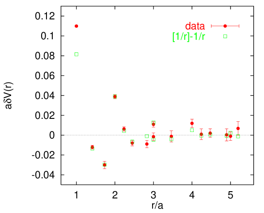
Figure 4.3: Comparison between the tree level expectation of violations of rotational invariance and lattice data at $\beta=6.4$.

The lattice potential at $\beta\leq 6.5$ is well described by the functional form [241],

$$V({\mathbf{r}})=V_{\mbox{\scriptsize cont}}(r)-l\delta V({\mathbf{r}}),\quad V_{\mbox{\scriptsize cont}}(r)=V_{0}+\sigma\,r-\frac{e}{r}+\frac{af}{r^{2}},$$ (4.68)

for separations as small as $r\geq\sqrt{3}a$. The $1/r^{2}$ term is not physically motivated but effectively parameterises the weakening of the coupling with the distance while the difference between tree level lattice and continuum perturbation theory results,

$$\delta V({\mathbf{r}})=\left[\frac{1}{\mathbf{r}}\right]-\frac{1}{r},$$ (4.69)

is used to quantify lattice artefacts. In Figure 4.3, we compare the theoretical difference $\delta V({\mathbf{r}})$ to $\delta V({\mathbf{r}})=[V_{\mbox{\scriptsize cont}}(r)-V({\mathbf{r}})]/l$, as calculated from the lattice data after determination of the fit parameters, $V_{0},\sigma,e,f$ and $l$, at $\beta=6.4$, in lattice units [166]. The Figure demonstrates that at the level of precision achieved, deviations from the continuous fit curve are statistically significant for $r\leq 4a$. Moreover, deviations from $V_{\mbox{\scriptsize cont}}(r)$ are qualitatively indeed very well parameterised by a multiple of the tree level difference.

4.7.3 Finite size effects

In lattice simulations the potential is determined on a torus with finite volume and the question of finite size effects (FSE) arises. Obviously, the ground state potential is affected by the infra-red cut-off. For instance, by exploiting the $r\leftrightarrow t$ symmetry of Euclidean space-time, it is clear from Appendix D that for the extreme case of a spatial extent smaller than the critical temperature of the deconfinement phase transition, any asymptotic string tension will disappear. The other source of FSE on Wilson loops is related to un-wanted interactions of source and anti-source around the periodic boundaries that will become negligible as $L_{\sigma}a\rightarrow\infty$: by unwrapping the spatial torus onto an infinite hyper-cubic lattice of cells with spatial periods, $L_{\sigma}a$, it becomes obvious that each charge at position ${\mathbf{r}}$ is accompanied by an infinite set of mirror charges at ${\mathbf{r}}_{\mathbf{n}}={\mathbf{r}}+{\mathbf{n}}L_{\sigma}a$, $n_{i}$ integer. For on-axis geometries, ${\mathbf{r}}=r\hat{\mathbf{\imath}}$, for instance, the closest mirror charge will be separated by a distance $L_{\sigma}a-r$ from the origin, followed by another charge at $L_{\sigma}a+r$. Therefore, in this case one would naïvely expect $V(r)=V(L_{\sigma}a-r)$. The symmetry, $V({\mathbf{r}})=V({\mathbf{r}}_{\mathbf{n}})$, is indeed reflected in the tree level weak coupling expansion results of Eqs. (4.51) and (4.52) and in fact holds to any order of perturbation theory for the singlet and octet potentials.

General considerations, based on the centre symmetry of the action which is discussed in Appendix D, however, lead us to expect the potential to be more robust against FSE than perturbation theory suggests. We will assume the source to be at position ${\mathbf{0}}$ and the anti-source to be at ${\mathbf{r}}$. The spatial connection, $\Psi_{\mathbf{r}}^{\dagger}$, built into a (smeared) Wilson loop is a linear combination of products of link variables along paths that have trivial winding number around the periodic boundaries. $\Psi_{\mathbf{r}}^{\dagger}$ has definite eigenvalues, $z_{i}\in Z_{N}$, with respect to the centre transformations associated with the three spatial directions. If we place the hyperplanes at which centre transformations, $z$, are applied at position ${\mathbf{x}}$ with $x_{i}\geq r_{i}$, i.e. such that they do not interfere with the shortest connection between the two test charges, we have $z_{i}=0$. However, a gauge transporter to a mirror charge at ${\mathbf{r}}_{\mathbf{n}}$ has the centre transformation property, $z_{i}=z^{n_{i}}$. Since the centre symmetry is both, a symmetry of the action as well as of the path integral measure, $z_{i}$ are conserved quantum numbers: the creation operator, $\Psi_{\mathbf{r}}$, only couples to mirror charges at distances in which all $n_{i}$’s are multiples of $N$. For on-axis separations in $SU(N)$ this means that the closest mirror charge contributing to the Wilson loop will be at a distance $NL_{\sigma}a-r$ [236, 242], rather than $L_{\sigma}a-r$ as the geometric argument alone or perturbation theory would have suggested. This suppression of FSE does obviously not work for Polyakov loop correlators in which the state of the gluonic flux tube remains unspecified. While in the standard weak coupling expansion the gauge group only influences the group theoretical pre-factors the centre charge affects the zero mode sector [252], ${\mathbf{q}}={\mathbf{0}}$ (that is suppressed by a power of the volume).

Numerical simulations of $SU(2)$ and $SU(3)$ gauge theories [242, 147] suggest that FSE on the static potential determined from Wilson loops, even at distances as big as $r=\sqrt{3}/2\,L_{\sigma}a$, are numerically undetectable on the 1 – 2 % level for $L_{\sigma}a>3\,r_{0}$. A reason besides the protection due to the centre symmetry for this finite size friendliness is the rather rapid on-set of the deconfinement phase transition which is first order in $SU(3)$ gauge theory. Full QCD, however, is less well explored yet and one might expect somewhat bigger FSE, at least for light sea quarks since the fermionic part of the action explicitly breaks centre symmetry. In particular, it might be hard to discriminate between breaking of the flux tube due to screening by sea quarks and FSE as reasons for an eventually flattening potential at large distances.

4.7.4 Sea quark effects

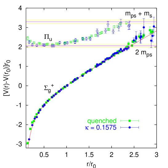
Figure 4.4: Comparison between quenched ($\beta=6.2$) and un-quenched $n_{f}=2$ ($\beta=5.6,\kappa=0.1575$) ground state and $\Pi_{u}$ potentials (from Ref. [248]).

When including sea quarks, one would expect two physical effects, one at large distances and one at small distances. While within the quenched approximation the number of quarks and anti-quarks are separately conserved, with sea quarks, only the difference (the baryon number) is a conserved quantity. Light quark anti-quark pairs can be created from the vacuum and in general transitions between a colour “string” state, spanned between two static sources, and two static-light mesons can occur. If the energy stored in the colour string between the sources exceeds a certain critical value at some distance, $r=r_{c}$, the string will “break” and decay into two static-light mesons, separated by a distance, $r$. Therefore, in the limit, $r\rightarrow\infty$, the ground state energy will stop rising with the distance and saturate at a constant level: the static sources will be completely screened by light quarks that pop up out of the vacuum.

The other effect will change the potential at short distances. While the vacuum polarisation due to gluons has an anti-screening effect on fundamental sources, sea quarks result in screening. Therefore, the running of the QCD coupling with the distance is slowed down with respect to the quenched approximation. This is for instance reflected in the factor, $11-2n_{f}$, within the perturbative $\beta$-function coefficient, $\beta_{0}$, of Eq. (C.1). When running the coupling from an infra-red hadronic reference scale down to short distances, the effective Coulomb strength in presence of sea quarks should, therefore, remain at a higher value than in the quenched case. It should be possible to detect this effect in the coefficient, $e$, within the Cornell parametrisation.

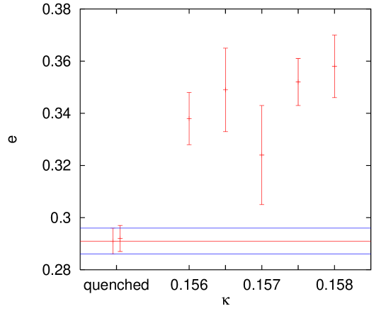
Figure 4.5: Sea quark mass dependence of the effective Coulomb strength of the static inter-quark potential.

In Figure 4.4, a recent comparison between the quenched ($\beta=6.2$) and $n_{f}=2$ static potential ($\beta=5.6$, $\kappa=0.1575$) by the $T\chi L$ collaboration at a sea quark mass, $m_{ud}\approx m_{s}/2$, is displayed [253, 248]. Besides the ground state potential, $\Sigma^{+}_{g}$, the lowest lying hybrid potential, $\Pi_{u}$, is shown. Estimates of masses of pairs of static-light mesons ($2m_{ps}$ and $m_{ps}+m_{s}$) into which the static-static systems can decay are also included into the Figure. The potentials have been matched to each other at a distance, $r=r_{0}\approx 0.5$ fm. Around $r\approx 2.3\,r_{0}\approx 1.15$ fm, both un-quenched potentials, $\Sigma_{g}^{+}$ and $\Pi_{u}$, are expected to become unstable. However, the data are not yet precise enough to resolve this effect. A similar comparison between the static potential and $2m_{ps}$ has first been performed by the UKQCD collaboration [254].

At small $r$ the un-quenched data points are found to be somewhat below their quenched counterparts: the effective Coulomb force indeed remains stronger. To quantify this effect, we fit the potentials [246, 255, 167, 248] (quenched at $\beta=6.0$ and $\beta=6.2$ and un-quenched at $\beta=5.6$ and various quark masses) for identical fit range in physical units, $0.4\,r_{0}<r<2\,r_{0}$, to the parametrisation of Eqs. (4.68), (4.69), with $f=0$. The resulting effective $e$ values from these four-parameter fits are displayed in Figure 4.5. Larger $\kappa$ values correspond to smaller quark masses. With two flavours of sea quarks of masses slightly larger than that of the strange quark, down to $m_{ud}\approx m_{s}/3$, the effective Coulomb strength is increased by 17 to 22 % which is not too far off from the most naïve expectation of 14 %, from the ratio, $\beta_{0}^{(n_{f}=0)}/\beta_{0}^{(n_{f}=2)}=33/29$. Within given errors the dependence on the sea quark mass cannot be resolved. However, one would expect this to be rather weak as the simulated quark masses are all much smaller than infra-red reference scales like $r_{0}^{-1}$. Similar results have been reported by the CP-PACS collaboration [247].

4.8 Beyond perturbation theory at short distances

The singlet potential,

$$V_{s}(q)=-C_{F}\frac{4\pi\alpha_{V}(q)}{q^{2}},$$ (4.70)

has been calculated to one loop long ago [225, 219] and now the two loop result is also known [258, 259, 260]. It is,

$$\alpha_{V,{\mbox{\scriptsize pert}}}(q)=\alpha_{\overline{MS}}(q)\left(1+a_{1}\alpha_{\overline{MS}}(q)+a_{2}\alpha_{\overline{MS}}^{2}+\cdots\right).$$ (4.71)

$a_{1}$ is defined in Eq. (4.62) and,

$$a_{2} = \left[\frac{4343}{18}+36\pi^{2}-\frac{9}{4}\pi^{4}+66\zeta(3)\right.$$

$$- \left.\left(\frac{1229}{27}+\frac{52}{3}\zeta(3)\right)n_{f}+\frac{100}{81}n_{f}^{2}\right]\frac{1}{16\pi^{2}}.$$

$\zeta(3)=1.2020569\ldots$ denotes the Riemann $\zeta$-function. For $n_{f}=5$ the numerical values are, $a_{1}=0.3802034\ldots$, $a_{2}=0.9868211\ldots$. Since $a_{2}\gg a_{1}$, perturbation theory seems to be rather slowly or badly convergent.

Naïvely, one might expect the perturbative calculation of the static QCD potential to be reliable in the limit of large energy scales, $q\simeq 1/r$, i.e at short distances. However, unlike in QED, the QCD potential is the ground state energy of a bound state composed of the two static colour sources and gluons. Bound state properties are associated with a characteristic scale, $\lambda$, which plays the rôle of an inverse gluonic coherence length. We identify $\lambda$ with the gap between ground state and first excitation. As we shall see in Section 5.2, for large $r$ this gap corresponds to the difference between a hybrid state and the ground state potential which, from the bosonic string picture, we expect to decrease at large distances like $\pi/r$. However, in the limit $r\rightarrow 0$ the gap will not diverge but saturate at a constant level that corresponds to the scalar glueball mass, $\lambda\approx 1.7$ GeV. Note that in QCD with light sea quarks it will be even smaller, of the order of the mass of two pions. The presence of such a low energy scale, affecting the short distance behaviour, can result in differences between the perturbatively calculated singlet potential and the static potential.

Non-perturbative $\Lambda^{4}/q^{4}$ power corrections to $\alpha_{V}$ that are due to the gluon condensate are indeed expected from the standard operator product expansion [261, 262, 263, 264]. Recently, this picture has been challenged by several authors [265, 266, 267, 268, 269, 270, 271, 272, 273, 274] who found various arguments in support of a term, proportional to $\Lambda^{2}/q^{2}$,

$$\alpha_{V}(q)=\alpha_{V,\mbox{\scriptsize pert}}(q)+c_{V}\frac{\Lambda^{2}_{\overline{MS}}}{q^{2}}+\cdots.$$ (4.73)

Lorentz invariance implies that no power law corrections of even lower order in $1/q$ exist. For the quenched case, where precise data exist down to lattice spacings as small as $a^{-1}\approx 5.5$ GeV, the lattice potential has been compared to perturbation theory and, indeed, a non-vanishing value, $c_{V}=4.8\pm 1.4$, has been found in Ref. [275] for $n_{f}=0$, after subtracting one loop perturbation theory. We briefly summarise this analysis below.

A Fourier transform of the momentum space potential yields,

$$V(r)=-C_{F}\frac{\alpha_{R}(1/r)}{r},$$ (4.74)

with [276, 260, 277, 275],

$$\alpha_{R}(1/r)=\alpha_{V,\mbox{\scriptsize pert}}(\mu)\left(1+\frac{\pi^{2}\beta_{0}^{2}}{3}\alpha_{V,\mbox{\scriptsize pert}}^{2}+\cdots\right)-2c_{V}\Lambda_{\overline{MS}}r^{2}+\cdots,$$ (4.75)

where $\mu=\exp(-\gamma_{E})/r$ and $\gamma_{E}=0.5772156\ldots$ denotes the Euler constant. While in the ultra-violet the effect of the $1/q^{2}$ power correction to $\alpha_{V}$ on $V(q)$ is suppressed by a factor, $1/q^{4}$, this suppression is proportional to $r$ only in position space [Eqs. (4.74) – (4.75)].

Figure 4.6: The quenched lattice potential and perturbation theory. The lattice data have been normalised such that $V(r_{0})=0$. The values $0.94\,r_{0}^{-1}$ and $0.77\,r_{0}^{-1}$ have been subtracted from the one and two loop formulae, respectively, to allow for comparison.

By employing a recursive lattice finite size technique [278, 142], the ALPHA collaboration has recently obtained a value for the running coupling in quenched $SU(3)$ QCD [103]. They quote the result,

$$\Lambda_{\overline{MS}}^{(0)}=0.602(48)/r_{0},$$ (4.76)

in units of the Sommer scale $r_{0}$. We use this result as an input to determine $\alpha_{\overline{MS}}$ at a high energy scale (1000 $r_{0}^{-1}$) and run it down from there to scales $\mu$, using the four loop renormalisation group equation, Eq. (3.22). Subsequently, the resulting $\alpha_{\overline{MS}}(\mu)$ is converted into $\alpha_{R}(e^{\gamma_{E}}\mu)$ to one and two loops via Eqs. (4.71) and (4.75) (with $c_{V}=0$), and the perturbative potential is determined. In Figure 4.6, we compare the result to lattice data. The disagreement is increased when going to higher order perturbation theory. Furthermore, the difference between perturbation theory and the non-perturbative determination is consistent with a linear term [275], as expected from Eqs. (4.74) and (4.75).

Because of the significant size of the coefficient, $a_{2}$, different ways of re-summing the series or performing the Fourier transform can result in somewhat different results and, therefore, in a different coefficient of the linear term, $-2C_{F}c_{V}\Lambda_{\overline{MS}}^{2}=(3.4\pm 1.0)\sigma$. Due to the non-convergent character of the perturbative series, subtracting the perturbative tail from a physical operator is never a well-defined procedure anyway. The ambiguity involved is related to renormalons that result from the interplay between perturbation theory and non-perturbative contributions — between the ultra-violet and the infra-red. By subtracting two loop perturbation theory, we find the linear term to have a slope about six times as big as the string tension. In contrast, tree level perturbation theory, with the coupling being treated as a free parameter, is compatible with the Cornell potential, i.e. results in the same linear slope, $\sigma$, for small and large distances.

4.9 String breaking

Having discussed the potential at very short distances, we shall re-examine the large distance behaviour. While a linear rise is expected in pure $SU(N)$ gauge theory, in full QCD the coupling of gluons to fundamental matter fields will result in a screening of inter-quark forces at large distances. However, this behaviour has not been detected so far in simulations involving sea quarks (cf. Figure 4.4). One reason might be that smeared Wilson loops are highly optimised to achieve enhanced overlap with the lowest lying string state and might, therefore, almost completely decouple [255] from the physical ground state at large $r$ that consists of two disjoint static-light mesons. Arguments based on the strong coupling expansion [279, 280] as well as on the bosonic string picture [281] support this suggestion. Investigating string breaking in full QCD is computationally very expensive as high statistics are required to resolve the potential in the large $r$ region of interest.

While string breaking has not been detected in the Wilson loop, the finite temperature potential, extracted from Polyakov line correlators at temperatures close to the deconfinement phase transition, exhibits a flattening, once sea quarks are included into the action [282, 283]. First indications of this effect have been reported as early as in 1988 [284]. Unlike Wilson loops, Polyakov line correlators automatically have non-vanishing overlap with any excitation, containing static quark and anti-quark, separated by a distance, $r$; in particular the static quarks can be accompanied by two disjoint sea quark loops, encircling the temporal boundaries, while in the Wilson loop case, co-propagating sea quarks are terminated by the spatial transporters at $x_{4}=0$ and $x_{4}=t$. The difference becomes perhaps most obvious in the loop expansion of Ref. [281]. Since for non-zero temperatures the finite temperature potential (or free energy) extracted from Polyakov line correlators will in general differ from the potential, extracted from Wilson loops, the situation is not yet satisfying.

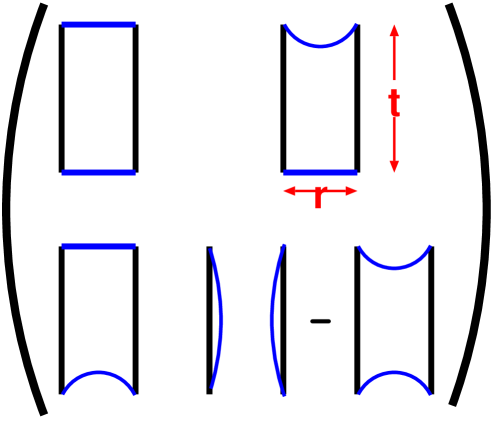
Figure 4.7: Graphical representation of the correlation matrix that is relevant for an investigation of string breaking in full QCD.

The first ambitious studies of string breaking in QCD using operators with better projection on the broken string state are at present being performed (see e.g. [254, 285, 286, 287, 248]). Such calculations involve diagonalisation of a two by two correlation matrix between string states and two pairs of static-light states. This matrix is visualised in Figure 4.7, where straight lines correspond to gauge transporters while curved lines represent light quark propagators that are obtained by inverting the fermionic matrix, $M$, of Eq. (3.11). The off-diagonal elements encode transitions between a string state with fixed ends and two static-light mesons while the bottom-right element represents two interacting static-light mesons, separated by a distance $r$. The second of the two contributions to this element corresponds to the exchange of a light meson. The situation becomes slightly more involved when the Dirac spin structure is taken into account.

Light quark propagators are normally just calculated for one source point to reduce the effort in terms of computer time and memory to a tolerable size. However, pairs of quark propagators emanating from different sites are required to calculate the bottom right element of the correlation matrix for various distances and times. Moreover, for a precise determination of expectation values of Wilson loops one usually exploits self-averaging: the average of the Wilson loop is not only taken over the Monte-Carlo generated ensemble of gauge configurations but also within each configuration; Wilson loops with different corner point coordinates are averaged, exploiting translational invariance. This practice is essential to reduce statistical fluctuations to an acceptable level. By use of refined stochastic estimator techniques [288] to calculate the all-to-all light quark propagators required for this purpose one will eventually be able to confirm string breaking at distances $r\approx 2.3\,r_{0}$.

Figure 4.8: The breaking of the adjoint string in $2+1$-dimensional $SU(2)$ gauge theory at a gauge coupling, $\beta=12$, in lattice units (from Ref. [151]).

In addition to the potential, breaking of closed strings (torelons) in QCD with sea quarks has been investigated [167, 255, 248]. Although the results suggest an effect, its statistical significance of $2.5$ standard deviations is not yet entirely convincing. While the situation in the case of interest is not settled yet, toy models have been investigated in three and four space-time dimensions. Similar to the situation of fundamental QCD colour sources being screened by sea quarks, one expects the string between adjoint sources in pure gauge theories to decay into a pair of gluelumps (or glueballinos), bound states between a static adjoint source (that can be thought to approximate a heavy gluino) and gluons (for a detailed discussion see e.g. Ref. [289]). Until recently, the situation was controversial: while in some early studies indications of the breaking of the adjoint string in four-dimensional $SU(2)$ and $SU(3)$ gauge theories have been reported [290, 291], in a later simulation of three-dimensional $SU(2)$ the broken string state has not been detected within Wilson loop correlators [292].

Figure 4.9: The breaking of the fundamental string in the $3+1$-dimensional $SU(2)$-Higgs model in physical units (from Ref. [293]). $\mu$ corresponds to the mass of a Higgs particle, bound to the static source.

In other studies a correlation matrix similar to that of Figure 4.7 between the string state and a two gluelump basis has been investigated. This was first done in four-dimensional $SU(3)$ gauge theory [294], followed by simulations of three-dimensional [295, 151] and four-dimensional [296, 297] $SU(2)$ gauge theories. The main result of the $d=3$ study of Ref. [151] is depicted in Figure 4.8. In addition to the ground state the first three excitations are included into the Figure. At small $r$, these resemble the first radial excitation of the string, two ground state gluelumps and one ground state gluelump plus an excited state gluelump, respectively. The horizontal lines indicate masses of pairs of isolated gluelumps where $E_{G}$ stands for the ground state and $E_{G}^{\prime}$ for the first excitation. A similar breaking pattern of the adjoint string has also been confirmed in four dimensional $SU(2)$ gauge theory [296, 297]. Studies of the breaking of the adjoint string have been preceded by investigations [298] of the breaking of the fundamental string in $SU(2)$ gauge theory with a Higgs field in the fundamental representation. The latest results from such simulations obtained in three [299] and four dimensions [300, 293]. confirm the expected screening of the static sources (see Figure 4.9).

In QCD one would expect a cross-over of the string state and the two static-light meson levels similar to the observations within the toy models considered above, even in the quenched approximation [301, 285]. How then can one distinguish the quenched scenario from the un-quenched one where the string is allowed to break? In the quenched case, the separate conservation of baryon and anti-baryon numbers implies that an open string state creation operator is orthogonal to a creation operator for the two static-light state. Therefore, each operator has zero overlap with the respective other state and only the assignment of the ground state to a particular operator will become interchanged around the would-be string breaking distance at which the two energy levels cross. Unlike the behaviour depicted in Figures 4.8 and 4.9, no energy gap at this distance will occur. Both, the string breaking distance and the associated energy gap, which is related to a phase shift in the mixing matrix of the un-quenched case, are relevant for an understanding of decay rates such as that of the $\Upsilon(4S)$ or $\Upsilon(5S)$ mesons into pairs of $B\overline{B}$ mesons.

4.10 Colour confinement

We have established the linearly rising potential in pure Yang-Mills gauge theories as a numerical fact and have made this behaviour plausible from strong coupling and string arguments. However, the dynamical question of how $SU(N)$ gauge theory as the theory of asymptotic freedom results in the formation of colour flux tubes with constant energy density per unit length remains un-answered. In the past decades, many explanations of the confinement mechanism have been proposed, most of which share the feature that topological excitations of the vacuum play a major rôle. These pictures include, among others, the dual superconductor scenario of confinement [302, 303, 304] and the centre vortex model [305, 211, 306, 307, 308, 309]. Depending on the underlying scenario, the excitations giving rise to confinement are thought to be magnetic monopoles, instantons, dyons, centre vortices, etc.. Different ideas are not necessarily exclusive. For instance, all fore-mentioned excitations are found to be correlated with each other in numerical as well as in some analytical studies, such that at present it seems to be rather a matter of personal preference which one to consider as more fundamental.

Figure 4.10: Electric field distribution between two static $SU(2)$ sources in the MA projection, in lattice units, $a\approx 0.081$ fm. The sources are located at the coordinates $(-7.5,0)a$ and $(7.5,0)a$.

Recently, the centre vortex model has enjoyed renewed attention [310]. In this picture, excitations that can be classified in accord with the centre group provide the disorder required to produce an area law of the Wegner-Wilson loop and, therefore, confinement. One striking feature is that — unlike monopole currents — centre vortices form gauge invariant two-dimensional objects, such that in four space-time dimensions, a linking number between a Wegner-Wilson loop and a centre vortex can unambiguously be defined, providing a geometric interpretation of the confinement mechanism [311].

We will only discuss the superconductor picture, which is based on the concept of electro-magnetic duality after an Abelian gauge projection that has originally been proposed by ’t Hooft and Mandelstam [302, 303]. The QCD vacuum is thought to behave analogously to an electrodynamic superconductor but with the rôles of electric and magnetic fields being interchanged: a condensate of magnetic monopoles expels electric fields from the vacuum. If one now puts electric charge and anti-charge into this medium, the electric flux that forms between them will be squeezed into a thin, eventually string-like, Abrikosov-Nielsen-Olesen vortex which results in linear confinement.

In all quantum field theories in which confinement has been proven, namely in compact $U(1)$ gauge theory, the Georgi-Glashow model and ${\mathcal{N}}=2$ SUSY Yang-Mills theories, this scenario is indeed realised. However, before one can apply this simple picture to QCD or $SU(N)$ gluodynamics one has to identify the relevant dynamical variables: it is not straight forward to generalise the electro-magnetic duality of a $U(1)$ gauge theory to $SU(N)$ where gluons carry colour charges. How can one define electric fields and dual fields in a gauge invariant way?

In the Georgi-Glashow model, the $SO(3)$ gauge symmetry is broken down to a residual $U(1)$ symmetry as the vacuum expectation value of the Higgs field becomes finite. It is currently unknown whether QCD provides a similar mechanism and various reductions of the $SU(N)$ symmetry have been conjectured. In this spirit, it has been proposed [304] to identify the monopoles in a $U(1)^{N-1}$ Cartan subgroup of the $SU(N)$ gauge theory after gauge fixing with respect to the off-diagonal $SU(N)/U(1)^{N-1}$ degrees of freedom. After such an Abelian gauge fixing QCD can be regarded as a theory of interacting photons, monopoles and matter fields (i.e. off-diagonal gluons and quarks). One might assume that the off-diagonal gluons do not affect long range interactions. This conjecture is known as Abelian dominance [312]. Abelian as well as monopole dominance are qualitatively realised in lattice studies of $SU(2)$ gauge theory [313, 314] in the maximally Abelian (MA) gauge projection [315], which appears to be a suitable gauge fixing condition.

Figure 4.11: Longitudinal electric field, $E=E_{\parallel}=|{\mathbf{E}}|$, and density of superconducting magnetic monopoles, $f$, in the centre plane between the sources.

In Figure 4.10, the electric field distribution between $SU(2)$ quarks, separated by a distance, $r=15a\approx 1.2$ fm, is displayed [316]. This distribution has been obtained within the MA gauge projection. The physical scale, $a\approx 0.081$ fm, derived from the value, $\sqrt{\sigma}=440$ MeV, for the string tension, is intended to serve as a guide to what one might expect in “real” QCD. Clearly, an elongated Abrikosov-Nielsen-Olesen vortex forms between the charges. In Figure 4.11, a cross section through the centre plane of this vortex is displayed. While the electric field strength decreases with the distance from the core, the modulus of the dual Ginsburg-Landau (GL) wave function, $f$, i.e. the density of superconducting magnetic monopoles, decreases towards the centre of the vortex where superconductivity breaks down. In this study the values $\lambda=0.15(2)$ fm and $\xi=0.25(3)$ fm have been obtained [316, 317] for penetration depth and GL coherence length, respectively. The ratio $\lambda/\xi=0.59(13)<1/\sqrt{2}$ classically corresponds to a type I superconductor very close to the border of type II behaviour, i.e. QCD flux tubes appear to weakly attract each other. However, for a final settlement on which side of the Abrikosov limit $SU(2)$ gauge theory lies, quantum corrections should be considered. A recent analysis of the same lattice data in terms of the classical four-dimensional Abelian Higgs model has resulted in similar conclusions [318]. For a more detailed discussion the reader is referred to Ref. [317].

5 More static potentials

We will discuss a variety of excitations of the pure gauge vacuum, such as hybrid potentials, glueballs, gluelumps, potentials between charges in non-fundamental representations and three-body potentials. In particular hybrid potentials, whose short range behaviour is related to the glueball and gluelump spectra, turn out to be relevant for quarkonia as they give rise to extra states that are not expected from the quark model. They are also related to relativistic correction terms to the static potential and determine the validity range of the adiabatic approximation as we shall see in Sections 6.3.5 and 6.5.4. Prior to discussing hybrid potentials, we shall introduce hybrid mesons.

5.1 Hybrid mesons

At the same time that QCD was invented it has been noticed [80] that the spectrum of this theory should in principle contain bound states without constituent quark content, the so-called glueballs, in addition to the mesons and baryons of the quark model. The question, however, arises what constitutes the difference between a flavour singlet meson that contains “sea” gluons and a glueball that contains sea quarks. In general such hypothetically pure states will mix with each other to yield the observed particle spectrum. Still, the possibility of gluonic excitations will result in extra levels within certain mass regions that would not have been expected from simplistic pure constituent quark model arguments. Moreover, glueballs with exotic, quark model forbidden, quantum numbers should exist. While in QCD the difference at least between non-exotic glueballs and flavour singlet mesons is somewhat obscured, the quenched approximation contains “pure” glueballs and the spectrum of such states may be used as an input for mixing models [319].

Another non-trivial spectroscopic consequence of the QCD vacuum structure are so-called hybrid mesons [320, 38, 321], i.e. mesons with “constituent” glue; by considering excitations of the glue, mesons can acquire exotic quantum numbers too. There is a slight problem with the notion of “constituent” glue. Neither the number of gluons is conserved, nor do they have a non-vanishing rest mass. How then can one define the difference between “constituent” and “sea” glue? Do not all mesons include a gluonic component? Even in the quenched approximation, where a glueball is a perfectly well defined object, we cannot easily switch off “sea” gluons to identify hybrids. What a “hybrid” is can only be understood within certain models like bag models [36, 38], the strong coupling lattice model [37, 41] or the flux tube model [43] that distinguish between hybrids and standard quark model states. Such models offer extensions of the quark model that help in classifying the observed hadron spectrum and can guide lattice simulations as well as sum rule calculations. In Section 6.5.4 we shall also see that in the framework of a semi-relativistic expansion the classification can be made more precise.

In full QCD an operator that is bilinear in the quark fields with given $J^{PC}$ content and flavour related quantum numbers isospin, $I$ and $I_{3}$, strangeness, charm and beauty will in general couple to all mesonic states within the given channel: in particular QCD makes no clear distinction between states with identical quantum numbers such as the flavour singlet states $\eta$, $\eta^{\prime}$, $\eta_{c}$ and $\eta_{b}$ and, for instance, pseudo-scalar glueballs: in the flavour singlet sector even the notion of a valence quark as opposed to a sea quark is, strictly speaking, ill defined. However, the $\eta_{c}$ is experimentally clearly distinct from an $\eta$, containing light constituent quarks; almost no mixing between the would-be pure $c\bar{c}$ and the corresponding pure light quark state of the naïve quark model occurs: while this is not an exact symmetry the assumption that the number of valence charm quarks and anti-quarks are separately conserved is a very good approximation of the physical situation. In this sense, one can still assign a flavour to individual constituent quarks.

We intend to create a meson, i.e. a state containing a quark, $q$, and an anti-quark, $\bar{q}^{\prime}$, with given $J^{PC}$ assignment. The most general creation operator that is bilinear in the quark fields is,

$$\sum_{{\mathbf{x}}}\bar{q}^{\prime\,\alpha}_{{\mathbf{x}},\mu}\Gamma_{\mu\nu}O^{\alpha\beta}_{\mathbf{x}}[U]q^{\beta}_{{\mathbf{0}},\nu},$$ (5.1)

where we have chosen the coordinates such that the quark is at the origin. $\alpha,\beta=1,2,3$ are colour and $\mu,\nu=1,\ldots,4$ Dirac indices. While $\Gamma$ determines the internal spin symmetry of the state, the function of the gauge fields, $O$, generates both, relative angular momentum of the quarks as well as excitations of the gluonic degrees of freedom. For trivial $O^{\alpha\beta}_{\mathbf{x}}=\delta_{\alpha\beta}\delta({\mathbf{x}})$, $\bar{q}\gamma_{5}q$ creates a pseudo-scalar meson ($J^{PC}=0^{-+}$) and $\bar{q}\gamma_{\mu}q$ a vector ($1^{--}$): in a colour and flavour singlet state without relative angular momentum of the quarks, Fermi statistics implies, $P=-1$ and $C=(-1)^{s}$ (in this special case ${\mathbf{J}}={\mathbf{S}}$). When one allows $q$ to differ from $\bar{q}^{\prime}$, the creation operator is no longer a charge eigenstate and scalars $\bar{q}^{\prime}q$ ($0^{+}$) as well as axial-vectors $\bar{q}^{\prime}\gamma_{5}\gamma_{\mu}q$ ($1^{+}$) can easily be created too.

In general, each $O_{\mathbf{x}}$ is a combination of gauge connections between ${\mathbf{0}}$ and ${\mathbf{x}}$. If one allows $O$ to have a non-trivial spatial distribution, angular momentum, ${\mathbf{L}}$, can be introduced. This can be achieved by the choice, $O_{\mathbf{x}}=Y_{ll_{3}}(\theta,\phi)U({\mathbf{x}})$, where $U({\mathbf{x}})$ denotes a Schwinger line connecting ${\mathbf{0}}$ with ${\mathbf{x}}$ and $Y_{ll_{3}}$ are the familiar spherical harmonics. By combining such angular excitations with the pseudo-scalar creation operator, all $q\bar{q}$ states, $J^{PC}=0^{-+},1^{+-},2^{-+},\ldots$, can be created while combination with a vector results in, $J^{PC}=0^{++},1^{--},1^{++},2^{--},2^{++},\ldots$. Note that $P=(-1)^{l+1},C=(-1)^{l+s}$.

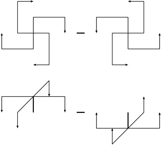
Figure 5.1: Lattice paths, $O$, with $O_{h}\otimes C$ quantum numbers, $T_{1}^{+-}$ and $T_{1}^{-+}$, respectively.

Let us now investigate the case, $O_{\mathbf{x}}^{\alpha\beta}=\delta({\mathbf{x}})B_{{\mathbf{0}},i}^{\alpha\beta}$. The chromo-magnetic field, ${\mathbf{B}}=\sum_{a}{\mathbf{B}}^{a}T^{a}$, transforms like an octet under gauge transformations and is traceless. It has the internal quantum numbers of an axial vector, $1^{+-}$, while the electric field ${\mathbf{E}}$ is a vector, $1^{--}$. Obviously, the combination, $\bar{q}^{\alpha}\gamma_{5}B_{i}^{\alpha\beta}q^{\beta}$, in which the quarks couple to a colour octet and interact with the magnetic gluon, shares the vector $J^{PC}=1^{--}$ spin assignment with the quark singlet state, $\bar{q}^{\alpha}\gamma_{i}q^{\alpha}$, while both, $\bar{q}^{\alpha}\gamma_{i}B_{i}^{\alpha\beta}q^{\beta}$ and $\bar{q}^{\alpha}\gamma_{5}q^{\alpha}$ are pseudo-scalars: It appears plausible to assume that the colour singlet operators have a better overlap with the physical ground state while the colour octet operators show an improved coupling with would-be hybrid excitations. We finally note that $\epsilon_{ijk}\bar{q}^{\alpha}\gamma_{j}B_{k}^{\alpha\beta}q^{\beta}$ results in a spin-exotic $1^{-+}$ assignment.

In general, one will employ a spatially extended creation operator. Two examples of such lattice operators, $O$, that incorporate bended gauge transporters (staples) which result in a non-trivial gluonic state are depicted in Figure 5.1. The first one corresponds to a lattice spin content, $T_{1}^{+-}$, while the second one is within the $T_{1}^{-+}$ representation of $O_{h}\otimes C$. The lowest lying continuum spin from which $T_{1}$ can be subduced is, $l=1$. In combining the above paths with various possible quark bilinears [324], the first operator projects onto mesons with $J^{PC}=0^{-+},{\mathbf{1}^{-+}},1^{--},2^{-+},\ldots$ while the second operator yields, $J^{PC}={\mathbf{0}^{+-}},1^{+-},1^{++},{\mathbf{2}^{+-}},\ldots$. Spin-exotic states have been indicated in bold. The lightest spin exotic mesons come out to have $J^{PC}=1^{-+}$ in studies of both, quenched QCD and QCD with two flavours of sea quarks [326, 327, 328]. As a next step mixing effects with possible $\pi f_{1}$ spin-exotic four-quark molecules should be considered.

5.2 Hybrid potentials

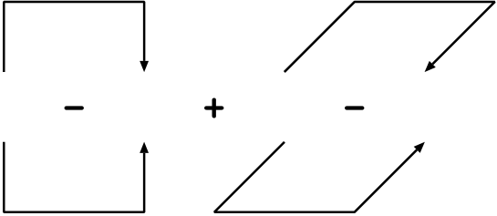
Figure 5.2: Creation operator for the $E_{u}$ hybrid potential.

While the distinction between a hybrid meson and an ordinary meson is not well defined, a hybrid potential with quantum numbers other than $\Sigma_{g}^{+}$ between static colour sources, separated by a distance ${\mathbf{r}}$ is clearly distinct from the ground state potential or its radial excitations of the ground state potential. Hybrid potentials can be classified in analogy to excitations of homonuclear diatomic molecules [176, 325]. The relevant symmetry group is $D_{\infty h}$ in the continuum and $D_{4h}$ on a cubic lattice (for on-axis separation of the sources). An angular momentum $\Lambda_{\hat{\mathbf{r}}}$ about the molecular axis can be assigned to the state. In addition, the state might transform evenly (gerade, g) or oddly (ungerade, u) under the combined parity of a charge inversion and a reflection about the midpoint of the axis, $\eta$. Finally, reflections with respect to a plane that includes the axis can be performed. For $\Lambda=|\Lambda_{\hat{\mathbf{r}}}|\neq 0$ such reflections just transform one state within a $\Lambda$-doublet into the other: $\Lambda_{\hat{\mathbf{r}}}\rightarrow-\Lambda_{\hat{\mathbf{r}}}$. However, for $\Lambda=0$, the transformation property under this reflection gives rise to an extra parity index, $\sigma_{v}$. Conventionally, the angular momentum is labelled by a capital Greek letter, $\Lambda=0,1,2,3\ldots=\Sigma,\Pi,\Delta,\Phi\ldots$. The straight line connection transforms in accord with the representation, $\Sigma_{g}^{+}$. In Figure 5.2, we have visualised a creation operator for the lattice $D_{4h}$ state, $E_{u}$, that can be subduced from the continuum representation, $\Pi_{u}$. The fact that staples pointing into positive and negative directions are subtracted from each other reflects the spin one nature of the state. Note that the combinations of Figure 5.1 contain similar elementary paths. The necessary group theory and lattice operators have been worked out in Ref. [231].

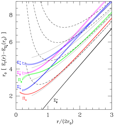
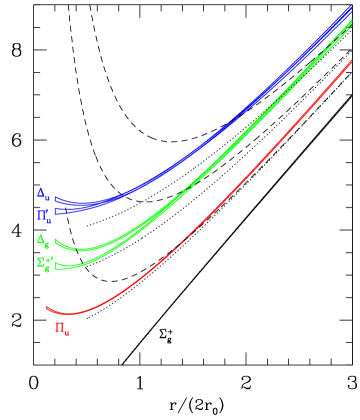
Figure 5.3: Hybrid excitations of the static $SU(3)$ potential (from Ref. [114]).

Lattice results for hybrid potentials have been obtained in $SU(2)$ [231, 146, 240] and $SU(3)$ [329, 330, 239, 331, 114, 332] gauge theories as well as in QCD with two flavours of sea quarks [167, 248]. For a recent review, see Ref. [333]. Employing the adiabatic and non-relativistic approximations for heavy quarks, one can estimate possible hybrid charmonia and bottomonia levels by solving the Schrödinger equation with such hybrid potentials. The only peculiarity is that the angular momentum, ${\mathbf{K}}={\mathbf{L}}+{\mathbf{S}}_{g}$, that couples to the spin of the quarks, ${\mathbf{S}}={\mathbf{S}}_{1}+{\mathbf{S}}_{2}$, to produce the total spin, ${\mathbf{J}}={\mathbf{K}}+{\mathbf{S}}$, differs from the angular momentum due to the relative motion of the quarks, ${\mathbf{L}}$. ${\mathbf{S}}_{g}$ denotes the spin of the gluonic flux tube whose projection onto the axis is, $\Lambda_{\hat{\mathbf{r}}}={\mathbf{S}}_{g}\hat{\mathbf{r}}$. Thus, $\langle k\Lambda|{\mathbf{S}}_{g}^{2}|k\Lambda\rangle\geq\Lambda(\Lambda+1)$ and $k\geq\Lambda$. Within the leading order Born-Oppenheimer approximation, ${\mathbf{K}}$ and $\Lambda$ are conserved, but not ${\mathbf{L}}$ or ${\mathbf{S}}_{g}$. The centrifugal term, $l(l+1)$ that appears in the radial Schrödinger equation, Eq. (A.2), has to be substituted by the correct factor [176], $\langle{\mathbf{L}}^{2}\rangle=k(k+1)-2\Lambda^{2}+\langle{\mathbf{S}}_{g}^{2}\rangle$.

Mass estimates of hybrid bottomonia, obtained in this way from hybrid potentials, can be found in Refs. [239, 331, 332]. Like in the case of light mesons the $1^{-+}$, $0^{+-}$ and $2^{+-}$ quarkonium spin-exotica, that are governed by the $\Pi_{u}$ potential in the adiabatic approximation, turn out to be the lightest ones. Within the quenched, non-relativistic and leading order Born-Oppenheimer approximations bottomonia hybrids come out to lie only slightly above the $B\overline{B}$ threshold. To this order in the semi-relativistic expansion, which does not yet incorporate spin sensitive terms, the masses of hybrid ${\mathbf{0}^{+-}}$, $0^{-+}$, ${\mathbf{1}^{-+}}$, $1^{--}$, $1^{+-}$, $1^{++}$, ${\mathbf{2}^{+-}}$ and $2^{-+}$ states are degenerate. It is clear, however, that for the non-exotic hybrids the use of an excited state potential within the Born-Oppenheimer approximation is at best dubious.

In Figure 5.3, the spectrum of hybrid potentials from the most comprehensive study so far [114] is displayed. Continuum limit extrapolated lattice results are indicated by pairs of solid curves while dotted curves correspond to the classical Nambu-Goto string expectation in four dimensions, Eq. (4.27). Dashed curves indicate $n\pi/r$ gaps, added to the ground state potential, the leading order contribution of the bosonic string picture. To guide the eye, the lowest lying states, $\Sigma_{g}^{+}$ and $\Pi_{u}$, are included into both plots. Note that a $\Phi_{u}$ interpretation of the $\Pi_{u}^{\prime}$ state cannot be excluded from the lattice data. However, as we shall see at the end of Section 5.3, other evidence speaks in favour of the $\Pi_{u}^{\prime}$ assignment. Most states are in clear disagreement with the simple model expectation up to distances as big as 3 fm where sub-leading terms of the string picture are rather small as the differences between dashed and dotted curves show. While this contrasts the findings of Ref. [213] for closed strings (torelons) and those of Ref. [146] for hybrid potentials, investigations of the ground state flux tubes between static sources indicate half widths of about 1 fm [242, 317]. Thus, although 3 fm is big in comparison with typical hadronic scales, the amplitude of string fluctuations is still quite large in relation to the longitudinal extent. Therefore, in an effective string representation the possibility of higher dimensional correction terms to the Nambu-Goto action might have to be considered.

The small distance behaviour exhibits a rich structure too and some states appear to try to become degenerate. In particular the change of curvature of the $\Pi_{g}$ potential at small $r$ appears puzzling. In the limit, $r\rightarrow 0$, the quarks combine to an octet or a singlet colour representation. The octet channel in which the sources explicitly couple to gluons should have relevance for the hybrid potentials that differ from the ground state by excitations of the gluonic flux tube. One might therefore assume that the short distance behaviour [334, 335] is determined by the perturbative octet potential $V_{o}(r)=-1/8V_{s}(r)$. This is in agreement with the observation that the curvature of all potentials (with the exception of $\Pi_{g}$) is smaller than and opposite in sign to the one of the ground state potential. Note that in the framework of potential NRQCD (pNRQCD), the hybrid potentials have also been predicted to follow $V_{o}$ to leading order, up to non-perturbative constants [335].

We would like to mention that in QED potentials can be classified in exactly the same way. Nonetheless, in the deconfined phase, that is realised in nature, the spectrum of excitations above the ground state Coulomb potential is continuous since photons of arbitrary momentum can be emitted. This is not so in QCD. However, the spectrum of QCD potentials will become continuous too above glueball pair radiation thresholds or, when allowing for light sea quarks, meson pair radiation thresholds.

5.3 Glueballs, glueballinos and hybrid potentials

In the limit, $r\rightarrow 0$, the cylindrical symmetry of a (hybrid) potential creation operator is enlarged to that of the full rotational group in three dimensions, $D_{\infty h}\subset O(3)\otimes C$ (or, on a cubic lattice, $D_{4h}\subset O_{h}\otimes C$). Irreducible representations of the subgroup with spin $\Lambda$ can be subduced from irreducible representations of the rotational group with spin $J\geq\Lambda$, as illustrated in Table 5.1. Note that $P=\sigma_{v}$, $C=\eta\sigma_{v}$. Moreover, states can be classified as singlets and octets in accord with their local gauge transformation properties. While a singlet state decouples from the temporal transporters within an $r=0$ “Wilson loop”, an octet state couples to a temporal Schwinger line in the adjoint representation. In the infinite mass limit, where spin can be neglected, the temporal transporter can be interpreted as the propagator of a static gluino, in analogy to fundamental lines representing a static quark. Consequently, the octet state is called a glueballino or gluelump [291, 289, 294, 334] while the singlet state that, neglecting quark pair creation, contains nothing but glue represents a glueball.

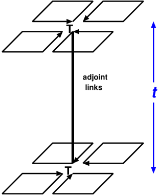
Figure 5.4: The gluelump correlation function, Eq. (5.2).

Gluelump masses can be extracted from the decay of the correlation function,

$$C(t)=\frac{1}{2N}\left\langle H^{a}_{{\mathbf{0}},t}[U^{A}_{\mathbf{0}}(t)]^{ab}H^{b}_{{\mathbf{0}},0}\right\rangle,$$ (5.2)

in Euclidean time. $U^{A}_{\mathbf{x}}(t)$ denotes an adjoint Schwinger line connecting the point $({\mathbf{x}},0)$ with $({\mathbf{x}},t)$ and $H$ is a local operator in the adjoint representation. The simplest example is, $H^{a}\propto B^{a}_{3}$, where $2\,\mbox{tr}\,(H^{F}T^{a})=\sum_{b}H^{b}2\,\mbox{tr}\,(T^{b}T^{a})=H^{a}$. This operator corresponds to an axial-vector, $J^{PC}=1^{+-}$, from which the $D_{\infty h}$ hybrid potentials, $\Pi_{u}$ and $\Sigma_{u}^{-}$, can be subduced in the limit, $r\rightarrow 0$. The three possible orthogonal choices of the direction $i$ of $B^{A}_{i}$ correspond to the dimensionality, $2J+1$, of the $J=1$ representation which is identical to the sum of dimensions of the subduced representations, $\Pi_{u}$ and $\Sigma_{u}^{-}$: $2+1$. From Eqs. (B.16), (3.7) and (3.8), we obtain lattice definitions of magnetic and electric field strength operators,

$$gB_{x,i}=\frac{1}{2ia^{2}}\epsilon_{ijk}\Pi_{x,jk},\quad gE_{x,i}=\frac{1}{2ia^{2}}\left(\Pi^{t}_{x,i}-\Pi^{t\dagger}_{x,i}\right),$$ (5.3)

that approximate the continuum limit up to ${\mathcal{O}}(a)$ lattice artefacts [${\mathcal{O}}(a^{2})$ in $SU(2)$ gauge theory]. In $SU(3)$ gauge theory one would preferably modify the above definitions,

$$B_{x,i}\rightarrow B^{\prime}_{x,i}=B_{x,i}-\mbox{Tr}(B_{x,i}){\mathbf{1}},\quad E_{x,i}\rightarrow E^{\prime}_{x,i}=E_{x,i}-\mbox{Tr}(E_{x,i}){\mathbf{1}},$$ (5.4)

to eliminate order $a$ scaling violations.

$$\Pi_{x,ij}=\frac{1}{4}\left(U_{x,i,j}+U_{x,-i,j}+U_{x,-i,-j}+U_{x,i,-j}\right)$$ (5.5)

denotes a “clover leaf” sum of four elementary plaquettes, Eq. (3.6), while,

$$\Pi^{t}_{x+\frac{a}{2}\hat{4},i}=\frac{1}{2}\left(U_{x,i,4}+U_{x,-i,4}\right),$$ (5.6)

is defined at half-integer values of the lattice time, $t/a$. Note that $\Pi_{x,ij}=\Pi^{\dagger}_{x,ji}$.

Table 5.1: What $O(3)\otimes C$ representation contains what $D_{\infty h}$ representations?

$\Lambda^{\sigma_{v}}_{\eta}$	$J^{PC}$
$\Sigma_{g}^{+}$	$0^{++},1^{--},2^{++},3^{--},\ldots$
$\Sigma_{g}^{-}$	$0^{--},1^{++},2^{--},3^{++},\ldots$
$\Sigma_{u}^{+}$	$0^{+-},1^{-+},2^{+-},3^{-+},\ldots$
$\Sigma_{u}^{-}$	$0^{-+},1^{+-},2^{-+},3^{+-},\ldots$
$\Pi_{g}$	$1^{++},1^{--},2^{++},2^{--},\ldots$
$\Pi_{u}$	$1^{+-},1^{-+},2^{+-},2^{-+},\ldots$
$\Delta_{g}$	$2^{++},2^{--},3^{++},3^{--},\ldots$
$\Delta_{u}$	$2^{+-},2^{-+},3^{+-},3^{-+},\ldots$

The correlation function of Eq. (5.2) is visualised in Figure 5.4. $1^{--}$ states can be created by operators, $H_{i}\propto E^{A}_{i}$, or by the operators, $H_{i}\propto\epsilon_{ijk}D^{A}_{j}B^{A}_{k}$. The latter operator is local in time and would preferably be used in lattice simulations. The five operators, $D_{i}^{A}B_{j}^{A}-\frac{1}{3}\delta_{ij}D_{i}^{A}B_{j}^{A}$, couple to $2^{--}$ states etc.. A table containing continuum creation operators for various quantum numbers can be found for instance in Ref. [335].

The correlation function, Eq. (5.2), can be rewritten in terms of operators in the fundamental representation by use of the completeness relation,

$$2\sum_{a}T^{a}_{\alpha\beta}T^{a}_{\gamma\delta}=\delta_{\alpha\delta}\delta_{\beta\gamma}-\frac{1}{N}\delta_{\alpha\beta}\delta_{\gamma\delta},$$ (5.7)

and the identity $(U^{A})^{ab}=2\,\mbox{tr}\,(UT^{a}U^{\dagger}T^{b})$. The result reads,

$$C(t)=\left\langle\mbox{Tr}_{F}\left[H^{F}_{{\mathbf{0}},t}U_{\mathbf{0}}(t)H^{F,{\dagger}}_{{\mathbf{0}},0}U^{\dagger}_{\mathbf{0}}(t)\right]\right\rangle,$$ (5.8)

where the disconnected part, $-\left\langle\mbox{Tr}\,H^{F}\mbox{Tr}\,H^{F,{\dagger}}\right\rangle$, vanishes due to, $\mbox{Tr}\,H^{F}=H^{a}\mbox{Tr}\,T^{a}=0$. The above correlation function resembles a “hybrid” Wilson loop in the limit, $r\rightarrow 0$. In this limit, the Wilson loop can be factorised into singlet and octet components,

$$\langle W_{\Psi}(r,t)\rangle=c_{1}e^{-m_{\mbox{\scriptsize gluelump}}(a)t}+c_{2}e^{-[m_{\mbox{\scriptsize glueball}}+V_{\Sigma_{g}^{+}}(r,a)]t}+\cdots\quad(r\rightarrow 0),$$ (5.9)

where on the lattice, $V_{\Sigma_{g}^{+}}(0,a)=\hat{V}_{\Sigma_{g}^{+}}(0)+V_{\mbox{\scriptsize self}}(a)=0$. At $r\gg a$, $\hat{V}_{\Sigma^{+}_{g}}(r)$ will approach the continuum potential. From the above representation we expect certain groups of hybrid potentials to become degenerate with each other as $r\rightarrow 0$ and to assume the mass of the lightest glueball or gluelump within the sector of allowed $J^{PC}$ quantum numbers that have overlap with the hybrid string creation operator, $\Psi^{\dagger}$.

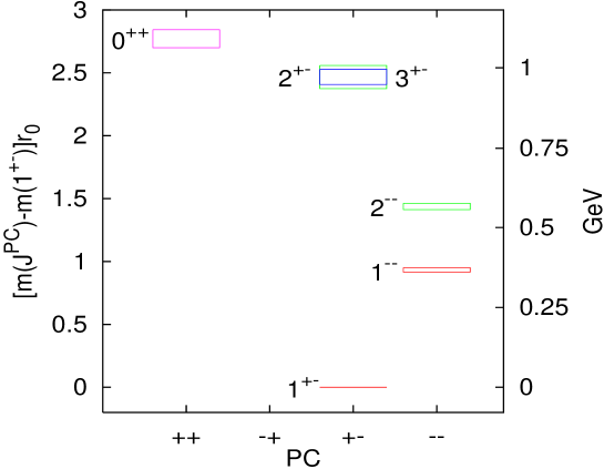
Figure 5.5: The lowest six $SU(3)$ gluelump states, extrapolated to the continuum limit [334].

Like static potentials, any gluelump mass will contain a finite contribution and a ($J^{PC}$ independent) contribution due to the self-energy of the static sources that will diverge in the continuum limit,

$$m_{\mbox{\scriptsize gluelump}}(a)=m_{\mbox{\scriptsize finite}}+m_{\mbox{\scriptsize self}}(a).$$ (5.10)

In order to obtain predictions on (hypothetical) glueballino masses, one has to substitute the (unphysical) self-energy by the rest mass of the constituent gluino in some appropriate scheme. Keeping this in mind, without additional input, only splittings of glueballino masses with respect to the ground state can be determined from lattice simulations of glueballino correlation functions. In analogy to Eq. (4.53), we obtain the tree level result,

$$m_{\mbox{\scriptsize self}}(a)=\frac{C_{A}}{C_{F}}\frac{V_{\mbox{\scriptsize self}}(a)}{2}=\frac{N^{2}}{N^{2}-1}V_{\mbox{\scriptsize self}}(a)>V_{\mbox{\scriptsize self}}(a):$$ (5.11)

the self-energy associated with the adjoint static source diverges faster than that of the two fundamental sources within the static potential. In view of this observation, it is clear that in the continuum limit, the glueball within Eq. (5.10) will be the lighter state and that the level ordering of the hybrid potentials at zero distance will be determined by the glueball spectrum. Increasing the separation a bit such that breaking of the rotational symmetry still remains small the generalised Wilson loop will contain a contribution which resembles the correlation function of a gluelump with a self-energy that is reduced as the adjoint source becomes smeared out into two fundamental sources. Depending on the size of gluelump level splittings in relation with the glueball spectrum, it is therefore quite possible that at small distances the spectrum of hybrid potentials will be guided by the ordering of gluelump levels before, towards $r\rightarrow 0$, the glueballs finally take over. Note that if we allow for sea quarks, flavour singlet mesons and meson pairs will become lighter than the respective glueball levels and determine the short distance behaviour.

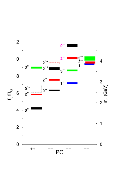
Figure 5.6: The glueball spectrum of $SU(3)$ gauge theory (from Ref. [116]).

What ordering of gluelump and glueball states do we expect? In the MIT bag model [37] for instance the lightest gluonic mode is the TE mode [320] ($J^{P}=1^{+}$), followed by the TM mode ($J^{P}=1-$). Hence, one might expect the axial-vector gluelump to be lighter than the vector gluelump. Such concepts have been generalised [336] by assuming that masses of particles increase with the lowest possible dimension of an operator with which the state in question can be created. While derivatives, $D$, have dimension $m$, quark creation operators, $q$, carry dimension $m^{3/2}$ and chromo electro-magnetic field operators, $E$ and $B$, dimension $m^{2}$. Only the $1^{+-}$ and the $1^{--}$ gluelumps can be created by operators of dimension two; all other states require derivatives or additional fields. Based on this simple picture, one would expect $1^{+-}$ to be the lighter state since a magnetic operator ($B$) excites a TE field. The next state would be $1^{--}$ ($E$), followed by $2^{--}$ ($DB$) and $2^{+-}$ ($DE$) and eventually states containing two derivatives ($3^{+-},3^{--}$) or two gluonic fields ($0^{++},2^{++},0^{-+},2^{-+}$) etc.. Indeed, the gluelump spectrum [334] of Figure 5.5 seems to follow this qualitative pattern that has also been predicted in Refs. [289, 335].

The lowest dimensional operator that can be used to create a glueball has dimension four. Here, we would expect the lowest states to be made up from two TE gluons ($BB$), coupling to $0^{++}$ and $2^{++}$, followed by $0^{-+}$ and $2^{-+}$, containing a TE plus a TM excitation, followed by $1^{++}$ and $3^{++}$ from dimension five $BDB$ operators (or an excited $0^{++}$ from two TE modes) etc.. However, as is revealed by Figure 5.6 [116], this simple picture fails after the first 3–4 states: the $1^{+-}$ is too light. The strong coupling model [41], in which one would expect the ordering $0^{++}$, $2^{++}$, $1^{+-}$ from the perimeter of the minimal loop required to create the state in question on the lattice, in contrast, fails to predict the low mass of the pseudo-scalar glueball. Of course an abundance of alternative qualitative and quantitative pictures of the QCD vacuum exists that result in somewhat different expectations. A detailed discussion of such models and the underlying assumptions is beyond the scope of the present article.

From the spectrum of glueballs and Table 5.1 we expect the $\Sigma_{g}^{+\prime}$ potential to be separated from the ground state by a scalar glueball mass $m(0^{++})$ at small distances, followed by three degenerate potentials $\Sigma_{g}^{+\prime\prime}$, $\Pi_{g}$ and $\Delta_{g}$ which will be separated from the ground state by $m(2^{++})$, $\Sigma_{u}^{-}$ separated by $m(0^{-+})$, another $m(0^{++\prime})$ triplet of potentials and a set of $\Pi_{u}$ and $\Sigma_{u}^{-\prime}$ states, separated by $m(1^{+-})$. In the regime of somewhat bigger $r$, which is dominated by gluelumps, we expect a low, almost degenerate pair of hybrid potentials, $\Pi_{u}$ and $\Sigma_{u}^{-}$, corresponding to $1^{+-}$, followed by a $\Pi_{g},\Sigma_{g}^{\prime}$ ($1^{--}$) pair and a $\Sigma_{g}^{-},\Pi_{g}^{\prime},\Delta_{g}$ ($2^{--}$) triplet. Indeed, Figure 5.3 reveals that the $\Sigma_{u}^{-}$ and $\Pi_{u}$ potentials are the lowest excitations at small $r$, and approaching each other. With $r\rightarrow 0$ we would expect the levels to cross as the value of $\Sigma_{u}^{-}$ will tend towards the ground state potential plus a pseudo-scalar glueball mass. Confirmation of this effect, however, requires lattice spacings that are sufficiently small to yield a gluelump mass exceeding that of the glueball in question. All the remaining levels are in complete agreement with the ordering and degeneracy expectations from the gluelump considerations too, with the exception of the $\Delta_{u}$ that comes out to be somewhat higher than its degenerate $2^{+-}$ $\Sigma_{u}^{+}$ and $\Pi_{u}^{\prime}$ partners. Unfortunately, no data on $\Pi_{g}^{\prime}$ exists, which we would have expected to become degenerate with $\Delta_{g}$ and $\Sigma_{g}^{-}$ at small $r$.

Lattice simulations [334] reveal that at spacings, $a^{-1}>2$ GeV, the sum of the scalar glueball mass and the ground state potential at the shortest accessible distance, $V_{\Sigma_{g}^{+}}(a)$, becomes smaller than the mass of the lightest ($1^{+-}$) gluelump. In the framework of effective field theories (see Section 6) a cut-off on gluon momenta is imposed. We conclude that as long as this cut-off does not exceed about 2 GeV hybrid related interactions are governed by the spectrum of gluelumps at short distance while when allowing for harder gluons, glueball channels will become increasingly important.

5.4 Casimir scaling

It is possible to determine the potential between colour sources not only in the fundamental representation (quarks) but in any representations of the gauge group. We have already discussed bound states between static adjoint sources (gluinos) and relativistic gluons above. Despite the availability of a wealth of information on fundamental potentials, only few lattice investigations of forces between sources in higher representations of gauge groups, $SU(N)$, exist. Most of these studies have been performed in $SU(2)$ gauge theory in three [337, 292, 295, 151] and four [338, 339, 340, 290, 341, 296, 297] space-time dimensions. Zero temperature results for $SU(3)$ can be found in Refs. [291, 294, 333, 342, 343, 344] while four-dimensional determinations of Polyakov line correlators in non-fundamental representation have been performed at finite temperature by Bernard [338, 345] for $SU(2)$ and Refs. [346, 347, 348, 283] for $SU(3)$ gauge theory. We have already discussed the $SU(2)$ results of Refs. [295, 151, 296] and the finite temperature results in the context of string breaking in Section 4.9 and shall focus on $d=4$ $SU(3)$ zero temperature simulations below.

Table 5.2: Group factors for $SU(3)$. $D$ is the dimension of the representation, $(p,q)$ are the weight factors, $z=\exp(2\pi i/3)$, and $d_{D}=C_{D}/C_{F}$ denotes ratios of Casimir factors.

$D$	$(p,q)$	$z^{p-q}$	$p+q$	$d_{D}$
3	$(1,0)$	$z$	1	1
8	$(1,1)$	1	2	2.25
6	$(2,0)$	$z^{*}$	2	2.5
$15a$	$(2,1)$	$z$	3	4
10	$(3,0)$	1	3	4.5
27	$(2,2)$	1	4	6
24	$(3,1)$	$z^{*}$	4	6.25
$15s$	$(4,0)$	$z$	4	7

For the static potential in the singlet channel in position space, tree level perturbation theory yields the result,

$$V(r,\mu)=-C_{D}\frac{\alpha_{s}}{r}+d_{D}V_{\mbox{\scriptsize self}}(\mu),$$ (5.12)

in analogy to Eq. (4.45). $D=1,3,6,8,10,\ldots$ labels the representation of $SU(3)$. $D=3$ corresponds to the fundamental representation, $F$, and $D=8$ to the adjoint representation, $A$. $C_{D}$ labels the corresponding quadratic Casimir operator, $C_{D}=\mbox{Tr}_{D}T_{a}^{D}T_{a}^{D}$, with the generators $T^{D}_{a}$ fulfilling the commutation relations of Eq. (B.7), $[T_{a}^{D},T_{b}^{D}]=if_{abc}T_{c}^{D}$. Table 5.2 contains all representations $D$, the corresponding weights $(p,q)$ for $p+q\leq 4$ and the ratios of Casimir factors, $d_{D}=C_{D}/C_{F}$. In $SU(3)$ we have $C_{F}=4/3$, and $z=\exp(2\pi i/3)$ denotes a third root of 1.

We denote group elements in the fundamental representation by $U$. The traces of $U$ in various representations, $W_{D}=\mbox{tr}\,U_{D}$, can easily be worked out,

$$W_{3} = \mbox{tr}\,U,$$ (5.13)

$$W_{8} = \left(|W_{3}|^{2}-1\right),$$ (5.14)

$$W_{6} = \frac{1}{2}\left[(\mbox{tr}\,U)^{2}+\mbox{tr}\,U^{2}\right],$$ (5.15)

$$W_{15a} = \mbox{tr}\,U^{*}\,W_{6}-\mbox{tr}\,U,$$ (5.16)

$$W_{10} = \frac{1}{6}\left[(\mbox{tr}\,U)^{3}+3\,\mbox{tr}\,U\,\mbox{tr}\,U^{2}+2\,\mbox{tr}\,U^{3}\right],$$ (5.17)

$$W_{24} = \mbox{tr}\,U^{*}\,W_{10}-W_{6},$$ (5.18)

$$W_{27} = |W_{6}|^{2}-|W_{3}|^{2},$$ (5.19)

$$W_{15s} = \frac{1}{24}\left[(\mbox{tr}\,U)^{4}+6(\mbox{tr}\,U)^{2}\mbox{tr}\,U^{2}+3(\mbox{tr}\,U^{2})^{2}\right.$$

$$+ \left.8\,\mbox{tr}\,U\,\mbox{tr}\,U^{3}+6\,\mbox{tr}\,U^{4}\right].$$

Note the difference, $\mbox{Tr}_{D}U_{D}=\frac{1}{D}\mbox{tr}\,U_{D}=\frac{1}{D}W_{D}$: the normalisation of $W_{D}$ differs from that of the Wilson loop of Eq. (4.1) by a factor $D$. Under the replacement, $U\rightarrow z\,U$, $W_{D}$ transforms like, $W_{D}\rightarrow z^{p-q}W_{D}$.

In Section 4.7.2 we have seen that for distances $r\geq 0.6\,r_{0}\approx$ 0.3 fm the fundamental potential is well described by the Cornell parametrisation,

$$V_{F}(r)=V_{0,F}-\frac{e_{F}}{r}+\sigma_{F}r.$$ (5.21)

Perturbation theory [Eq. (5.12)] tells us, $V_{0,D}\approx d_{D}V_{0,F}$ and $e_{D}\approx d_{D}e_{F}$. While the fundamental potential in pure gauge theories linearly rises ad infinitum, the adjoint potential will be screened by gluons and, at sufficiently large distances, decay into two disjoint gluelumps. This string breaking has indeed been confirmed in numerical studies [347, 348, 294, 295, 151, 296, 297]. Therefore, strictly speaking, the adjoint string tension is zero. In fact, all charges in higher than the fundamental representation will be at least partially screened by the background gluons. For instance, ${\mathbf{6}}\otimes{\mathbf{8}}={\mathbf{2}}{\mathbf{4}}\oplus{\mathbf{1}}{\mathbf{5}}{\mathbf{a}}^{*}\oplus{\mathbf{6}}\oplus{\mathbf{3}}^{*}$: in interacting with the glue, the sextet potential obtains a fundamental (${\mathbf{3}}^{*}$) component. A simple rule, related to the centre of the group, is reflected in Eqs. (5.13) – (5.4): wherever $z^{p-q}=1$, the source will be reduced into a singlet component at large distances while, wherever $z^{p-q}=z(z^{*})$, it will be screened, up to a residual (anti-)triplet component, i.e. one can easily read off the asymptotic string tension ($0$ or $\sigma_{F}$) from the third column of Table 5.2, rather than having to multiply and reduce representations. As a result, the self adjoint representations, ${\mathbf{8}}$ and ${\mathbf{2}}{\mathbf{7}}$, as well as the representation, ${\mathbf{1}}{\mathbf{0}}$, will be completely screened while in all other representations with $p+q\leq 4$ a residual fundamental component survives. The same argument, applied to $SU(2)$, results in the prediction that all odd-dimensional (bosonic) representations are completely screened while all even-dimensional (fermionic) representations will tend towards the fundamental string tension at large distances.

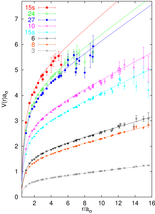
Figure 5.7: Static potentials between sources in various representations of $SU(3)$ in lattice units, $a_{\sigma}\approx 0.085$ fm.

While the string tension approaches either $0$ or $\sigma_{F}$ at very large distances, in an intermediate range an approximate linear behaviour is found [340, 290, 291, 348, 294, 333, 342, 295, 151, 343], such that one might speculate whether in this region the Casimir scaling hypothesis [337], $\sigma_{D}\approx d_{D}\sigma_{F}$, that is exact in two-dimensional QCD, holds. This hypothesis has been challenged by the fact that in all but two [343, 344] lattice simulations the expected Casimir slope is under-estimated. Motivated by this observation other models have been suggested, like scaling in proportion with the number of fundamental flux tubes embedded into the higher representation vortex [$p+q$ in $SU(3)$] [333, 343], which happens to coincide with Casimir scaling in the large $N$ limit. Casimir scaling and flux counting predictions, at least for the lower dimensional representations, are close to each other, such that discriminating between them represents a numerical challenge.

The latest lattice results for $SU(3)$ gauge theory from Ref. [343] are displayed in Figure 5.7 in lattice units, $a_{\sigma}\approx r_{0}/6\approx 0.085$ fm. Note, that the raw lattice data are displayed and no self-energy pieces have been subtracted. The data have been obtained on lattices with an anisotropic Wilson action and tiny temporal lattice spacing, $a_{\tau}^{-1}\approx 4a_{\sigma}^{-1}\approx 24\,r_{0}^{-1}\approx 9.5$ GeV. The fundamental potential for distances, $r\geq 0.6~{}r_{0}$, has been fitted to Eq. (5.21). The expectations on the potentials, $V_{D}(r)$, which are displayed in the Figure, correspond to the resulting fit curve, multiplied by the factors $d_{D}$. As one can see, up to distances where the signal disappears into noise or the string might break, the data are well described by the Casimir scaling assumption. Since this study has been performed on the finest lattice resolution so far, it can very well be that the underestimation of the Casimir scaling prediction of previous studies is a lattice artefact that will disappear after an extrapolation to the continuum limit. Indeed, a close inspection of data for the three-dimensional $SU(2)$ case [292, 295, 151] shows the tendency that the Casimir scaling expectation is approached from below with decreasing lattice spacing. It is still an open question whether Casimir scaling only holds approximately or if it is exact for distances smaller than the corresponding string breaking scales.

5.5 Three-body potentials

Although weak decays turn the phenomenology of hadrons composed of three or more heavy quarks experimentally unpromising, predicting properties of such heavy quark systems is the starting point for understanding multi-quark bound states from QCD and, eventually, nuclear physics. The first steps into the latter direction of including light quarks have been done by Michael and Pennanen who investigate systems composed of two light and two heavy quarks [285] or the even more ambitious study of the $uuddss$ $H$-dibaryon, containing six light valence quarks by Wetzorke and collaborators [350]. Forces between three and more static sources are not only interesting to guide the phenomenology of multi-quark states and to develop and test the lattice methodology required in this context but also for model builders: can multi-quark interactions be understood in terms of two-body interactions or have genuine three- and many-body effects to be considered? Hadronisation models for instance, which intend to explain the formation of hadronic jets in high energy scattering experiments, crucially rely on a factorisation hypothesis.

In the past years the Helsinki group has made extensive investigations of systems composed of four static $SU(2)$ sources [351, 352, 353, 354, 355], where no distinction between quarks and anti-quarks exists. These systems, therefore, have the capacity to approximate both, meson-meson and baryon-baryon interactions in QCD. The lack of difference between baryons and mesons is of course a serious limitation when trying to understand multi-quark interactions. For instance, unlike in $SU(3)$ where just two different pairings within four quark systems are possible, in $SU(2)$ three different ways of dividing the system into two colour singlets are viable: combinatorially, the four quark system finds its generalisation in $SU(3)$ systems composed of six quarks; however, geometrically, $q\bar{q}q\bar{q}$ systems come closer. Here, we will restrict our discussion to the simpler case of three quarks in QCD.

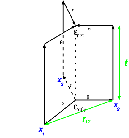
Figure 5.8: A baryonic Wilson loop.

In analogy to the standard (mesonic) Wilson loop, in $SU(N)$ ($N\geq 3$) gauge theories gauge invariant baryonic Wilson loops, $W_{Nq}$, can be defined. for the case of $SU(3)$ the binding energy of a system of three static quarks at positions ${\mathbf{x}}_{1}$, ${\mathbf{x}}_{2}$, and ${\mathbf{x}}_{3}$ (baryonic potential, $V_{3q}$) can be extracted in the limit, $t\rightarrow\infty$. The baryonic Wilson loop is composed of three staples, $U^{i}$, $i=1,2,3$, whose colour indices are contracted at Euclidean times $0$ and $t$ by completely antisymmetric tensors,

$$W_{3q}({\mathbf{x}}_{1},{\mathbf{x}}_{2},{\mathbf{x}_{3}};t)=\frac{1}{3!}\epsilon_{\alpha\beta\gamma}\epsilon_{\rho\sigma\tau}U^{1}_{\alpha\rho}U^{2}_{\beta\sigma}U^{3}_{\gamma\tau}.$$ (5.22)

The definition of the staples, $U^{i}$, is evident from Figure 5.8. The spatial parts of the baryonic loop will in general be composed of fat or smeared links for enhanced overlap with the physical ground state. The contraction of the colour indices can take place at a spatial coordinate at time $t$ that differs from that at time $0$. Moreover, the contraction points do not necessarily have to differ from the static quark positions, ${\mathbf{x}}_{i}$. In the limit, ${\mathbf{r}}_{12}\rightarrow 0$, two quarks combine to an anti-triplet, ${\mathbf{3}}\otimes{\mathbf{3}}={\mathbf{3}}^{*}\oplus{\mathbf{6}}$, that interacts with the remaining quark at position ${\mathbf{x}}_{3}$: in this limit the baryonic Wilson loop becomes a mesonic Wilson loop.

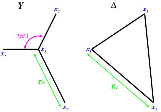
Figure 5.9: The star geometry with, $r_{Y}=\sum_{i}r_{iS}$, and the $\Delta$ geometry with, $r_{\Delta}=\sum_{i>j}r_{ij}$.

The colour factor that accompanies the tree level perturbative result reads,

$$\frac{1}{3!}\epsilon_{\alpha\beta\gamma}\epsilon_{\alpha\sigma\tau}T^{a}_{\beta\sigma}T^{a}_{\gamma\tau}=-\frac{1}{2}\mbox{Tr}\left(T^{a}T^{a}\right)=-\frac{C_{F}}{2}.$$ (5.23)

With another minus sign due to the different relative orientation of the quark lines with respect to a mesonic Wilson loop we arrive at the tree level relation,

$$V_{3q}({\mathbf{x}}_{1},{\mathbf{x}}_{2},{\mathbf{x}}_{3})=\frac{1}{2}\left[V({\mathbf{r}}_{12})+V({\mathbf{r}}_{23})+V({\mathbf{r}}_{31})\right],$$ (5.24)

between baryonic and mesonic potentials. For the non-perturbative long range part, two models compete with each other, which we shall refer to as the star (or $Y$) and the $\Delta$ laws. The first model originates from strong coupling and area minimisation considerations [356, 357, 44, 358, 359]. The solution of the problem of finding the shortest connecting path is well known for the case of three points, i.e. for a planar geometry; three straight lines emanating from the quarks will meet at an angle of $2\pi/3$ at a central Steiner point, ${\mathbf{x}}_{S}$ (Figure 5.9). Unless one of the angles within the baryonic triangle exceeds the value $2\pi/3$, in which case a linear geometry will be preferred, the resulting minimal area configuration resembles a Mercedes star shape. In this case, we expect the baryonic potential to be described by parameters extracted from a Cornell fit, Eq. (5.21), to the mesonic potential, in the following way,

$$V_{3q}({\mathbf{x}}_{1},{\mathbf{x}}_{2},{\mathbf{x}}_{3})\approx\frac{3}{2}V_{0}-\frac{e}{2}\sum_{i>j}\frac{1}{r_{ij}}+\sigma\,r_{Y},$$ (5.25)

where we have approximated the terms associated with the short range behaviour by the perturbative expectation.

Figure 5.10: Three quark potential obtained on an equilateral triangle, $r_{ij}=r_{12}=r_{23}=r_{31}$, in $SU(3)$ gauge theory with Wilson action at $\beta=6.0$ [360].

The competing contender is the $\Delta$ law [361, 362],

$$V_{3q}({\mathbf{x}}_{1},{\mathbf{x}}_{2},{\mathbf{x}}_{3})\approx\frac{3}{2}V_{0}-\frac{e}{2}\sum_{i>j}\frac{1}{r_{ij}}+\frac{\sigma}{2}r_{\Delta}:$$ (5.26)

although obviously, $r_{\Delta}>r_{Y}$, in this case each static quark line is shared by two surfaces which, depending on the underlying model [362], can result in a pre-factor, $1/2$, to avoid over-counting. Since $r_{\Delta}/2\leq r_{Y}$, this might then be the dominant configuration. Obviously, whenever the three quarks belong to a straight line, the two models yield identical predictions. The biggest difference is encountered for the case of an equilateral triangle where the predictions disagree by about 15 %,

$$r_{Y}=\sqrt{3}\,r_{ij}=\frac{2}{\sqrt{3}}\frac{r_{\Delta}}{2}.$$ (5.27)

Only very few lattice results [363, 364, 365] on baryonic potential existed so far, with statistical errors too big to rule out either possibility. In an as yet unpublished study [360], however, clear evidence in support of the $\Delta$ law has been found. The result for an equilateral triangle in lattice units is displayed in Figure 5.10 for $SU(3)$ gauge theory with Wilson action at $\beta=6.0$ ($a\approx 0.094$ fm): the data perfectly agree with the simple expectation, $V_{3q}=(3/2)V_{q\bar{q}}(r_{12})$, which, like the ratios between potentials between charges in different representations of the gauge group presented above, happens to coincide with tree level (and higher order) perturbation theory, Eq. (5.24).

It is interesting to notice that phenomenological fits of the baryon spectrum, for instance in the framework of relativised quark models [59] in which the $Y$ law is assumed, yield a string tension that is reduced by about 20 % [366], compared to the corresponding mesonic result. This is fairly consistent with the lattice results for the configuration of the equilateral triangle presented above. We conclude that while the agreement of the lattice data with the $\Delta$ law is appealing the question whether the $\Delta$ law holds or an approximate $Y$ law with a reduced string tension is satisfied cannot conclusively be answered until additional source geometries have been investigated.

6 Relativistic corrections

In this Section we attempt to bridge the gap between QCD dynamics of heavy quark bound states and potential models. We will sketch the derivation of a quantum mechanical Hamiltonian, containing the static potential as well as semi-relativistic correction terms. To leading order this has been pioneered by Wilson, Brown and Weisberger [1, 175] some 20 years ago. As soon as the approach was generalised to higher orders [22, 23, 25] in the inverse heavy quark mass, $m^{-1}$, or, better, relative heavy quark velocity, $v$, certain inconsistencies appeared between the non-perturbatively derived general form of the interaction and a direct perturbative evaluation [367] of the potential between two heavy quark sources at order $\alpha_{s}^{2}/m^{2}$.

A lot of progress in the understanding of effective theories, in particular in the matching of low energy theories to QCD has been achieved since then, and the problem is now understood [28] and removed. Motivated by these developments, we choose to start our discussion from non-relativistic QCD (NRQCD) in the continuum and on the lattice, before we address relativistic corrections to the heavy quark potential. Special emphasis is put on the matching problem. We shall also see that the validity of the adiabatic approximation is very closely tied to that of the non-relativistic expansion. Finally, lattice results on the heavy quark interaction will be presented.

6.1 NRQCD

6.1.1 The problem

We wish to consider mesonic bound states that contain two heavy quarks, namely the $J/\psi$, $\Upsilon$ and $B_{c}$ quarkonia families. Typical binding energies, $\overline{\Lambda}$, turn out to be a few hundred MeV, similar to systems that are entirely composed of light constituent quarks. The quark mass, $m$, however, is much larger. This difference in scales results in complications when evaluating physical properties. In a standard lattice computation for instance one has to work at lattice cut-offs, $a\ll m^{-1}$, in order to resolve the heavy quark while at the same time the box size has to be kept sufficiently large to resolve the scales that are relevant for the dynamics of the bound state like the binding energy, $L_{\sigma}a\gg\overline{\Lambda}^{-1}$. This results in a prohibitively large number of lattice sites that seems physically unnecessary since the scale, $m\gg\overline{\Lambda}$, appears to be rather irrelevant for the quarkonia level splittings (cf. Section 2.2). Indeed, closer inspection shows that only the temporal lattice spacing, $a_{\tau}\ll m^{-1}$, is limited by the quark mass. The computational effort becomes tolerable when an anisotropy, $a_{\tau}/a_{\sigma}\approx\overline{\Lambda}/m$, is introduced.

The two scale problem can even be turned into a virtue within an effective field theory formalism. The strategy would be to integrate out the ultra-violet behaviour at scales, $\mu\approx m$, into local Wilson coefficients of an effective low energy action that encodes the information relevant for bound state properties. Heavy quark effective theory [368, 369, 370] (HQET) for instance is a very effective framework for the calculation of properties of systems containing one heavy quark. The strategy is to write down an effective action that approximates QCD to a given power $\nu$ in $m^{-1}$. In general, the effective Lagrangian will then contain all operators of dimensions smaller than or equal to that of $m^{\nu+4}$. The coefficients that accompany these terms can be determined by matching on-shell Green functions, calculated in the effective theory, to those calculated in QCD, in the ultra-violet. This can be done for example in perturbation theory which is supposed to be applicable as long as, $\mu\gg\Lambda_{QCD}$. The tree level matching coefficients can be obtained by formally expanding the Dirac Lagrangian in terms of $m^{-1}$.

Although NRQCD [33], that applies to systems containing two heavy quarks, is somewhat more involved it has in fact been formulated earlier than HQET. The power counting scheme required for quarkonia differs from the one used in heavy-light systems. This is related to the fact that in the lowest order HQET Lagrangian, heavy quarks with non-vanishing relative velocity decouple from each other. In order to allow for interactions, a kinetic term, $p^{2}/2m$, is required that causes changes of the relative quark velocity, $v$. Therefore, the lowest order effective Lagrangian depends explicitly on the quark mass, $m$, in a way that cannot be absorbed into simple field redefinitions: the HQET power counting is obscured and a different expansion parameter is required.

As an alternative it has been suggested to expand the effective Lagrangian in terms of the quark velocity, $v$. One consequence is that in NRQCD a hierarchy of scales, $m\gg mv\gg mv^{2}\gg\ldots$, is introduced. The binding energy, $\overline{\Lambda}$, is of the order of the ultra-soft scale, $mv^{2}$, while the typical three-momenta exchanged, $mv$, are soft. The hard scale, $m$, is integrated out into matching coefficients, $c_{i}(\mu/m,\alpha_{s})$, at a scale $m\geq\mu\geq mv$. With the hierarchy of scales comes the possibility of a hierarchy of effective theories: after integrating out the soft scale, $mv$, another effective field theory, potential NRQCD (pNRQCD), can be formulated [371, 372, 335].

Figure 6.1: Determination of the relevant coupling for hypothetical $t\bar{t}$ bound states.

Table 6.1: Hard, soft and ultra-soft scale estimates.

	$J/\psi$	$\Upsilon$	$t\bar{t}$	$e^{+}e^{-}$
$m$	1.4 GeV	4.7 GeV	175 GeV	511 keV
$mv$	0.7 GeV	1.3 GeV	45 GeV	3.7 keV
$mv^{2}$	0.4 GeV	0.4 GeV	12 GeV	0.027 keV
$v$	0.5	0.29	0.26	0.007

In Table 6.1, estimates of the three scales for the charmonium, bottomonium and (unstable and therefore hypothetical) toponium ground states from a potential calculation are listed. For comparison, we include the corresponding estimates for positronium. The top quark is so heavy that for our estimate only a Coulomb like potential needs to be considered. In this case, $V(r)=-C_{F}\alpha_{R}/r$, and one easily obtains from the virial theorem [Eq. (A.4) with $\nu=1$], $\langle V\rangle=-2\langle T\rangle=2E_{1}$, using $E_{1}=-mC_{F}^{2}\alpha_{R}^{2}/4$,

$$\frac{\langle v^{2}\rangle}{c^{2}}=C_{F}^{2}\alpha_{R}^{2},\quad\frac{\langle r^{-1}\rangle}{c}=\frac{1}{2}mC_{F}\alpha_{R}.$$ (6.1)

In Figure 6.1, $2/(C_{F}m_{t})\langle r^{-1}\rangle$ and $\alpha_{R}$ are plotted as functions of $r$. The upper $n_{f}=5$ curve has been obtained from the input value, $\alpha_{\overline{MS}}(m_{Z})=0.1214(31)$, from $e^{+}e^{-}$ experiments at LEP and SLAC [82], by use of Eqs. (4.71) and (4.75). The quenched, $n_{f}=0$, estimate has been calculated by use of the lattice result of Ref. [103], displayed in Eq. (4.76). The intersects correspond to the values, $\alpha_{R}^{(0)}(17\,\mbox{GeV})\approx 0.145$, and, $\alpha^{(5)}_{R}(23\,\mbox{GeV})\approx 0.20$. The estimates quoted in Table 6.1 were obtained using the latter ($n_{f}=5$) result. The matching coefficients between QCD and NRQCD are calculable in perturbation theory as long as $m\gg\Lambda_{QCD}$ while perturbative matching between NRQCD and pNRQCD can be performed whenever $mv\gg\Lambda_{QCD}$. However, given the numbers in the Table, a reliable perturbative determination of the matching coefficients for charmonia states appears to be doubtful while for top quarks even perturbative pNRQCD should be applicable, up to power corrections [274, 373, 33].

6.1.2 The NRQCD Lagrangian and power counting

In order to derive an effective field theory that includes a kinetic term in its leading order Lagrangian, we introduce a second dimension $[v]=c$, in addition to the mass, and expand the Lagrangian formally in terms of [374, 375] $1/c$. As a result, time is measured in different units than space: $t=x_{4}/c$, $\partial_{t}=c\partial_{4}$ and $D_{t}=cD_{4}=\partial_{t}-iA_{4}$. The spatial covariant derivative reads, $D_{i}=\partial_{i}-\frac{i}{c}A_{i}$. The kinetic term, $\mbox{tr}\,F_{\mu\nu}F_{\mu\nu}$, has dimension $m^{4}c^{6}$. We define,

$$S=\frac{1}{c}\int\!d^{3}x\,\int\!dt\,{\mathcal{L}},$$ (6.2)

where,

$${\mathcal{L}}=\frac{1}{2g^{2}}\mbox{tr}\,F_{\mu\nu}F_{\mu\nu}+\bar{q}[{\mathbf{\gamma}}\cdot{\mathbf{D}}c+\gamma_{4}D_{t}+mc^{2}]q.$$ (6.3)

In order to make the leading order NRQCD Lagrange density independent of $c$, we have rescaled ${\mathcal{L}}$ by an overall factor, $c$ [Eq. (6.2)], which is compensated in the fermionic part by rescaling the fermion fields, $q$ and $\bar{q}$, by factors, $\sqrt{c}$.

At tree level a classical derivation of the NRQCD Lagrangian from the Dirac Lagrangian is possible by means of the Foldy-Wouthuysen-Tani (FWT) rotation [376, 377]: one starts from the Dirac basis in which $\gamma_{4}$ is diagonal and then, order by order in ${\mathbf{p}}/(mc)$, the fermion kernel is iteratively block diagonalised into separate non-interacting quark and anti-quark sectors. The first order transformation takes the form,

$$q\rightarrow\exp\left(\frac{{\mathbf{\gamma}}\cdot{\mathbf{p}}}{2mc}\right)q,$$ (6.4)

which happens to be the correct expression to all orders in the free field case. Subsequently, the rest mass can be removed by rescaling the (anti-)fermion fields with the factor, $\exp(\pm mc^{2}t)$. For details see e.g. Ref. [35]. We choose the decomposition,

$$q=\left(\begin{array}[]{c}\psi\\ \chi\end{array}\right),$$ (6.5)

of the Dirac spinor in the FWT basis into quark and anti-quark Pauli spinors.

The resulting effective Lagrangian to order $c^{-2}$ for the two-particle sector reads,

$${\mathcal{L}}_{\psi}+{\mathcal{L}}_{\chi}=-\psi^{\dagger}\left[D_{4}+H_{\psi}\right]\psi-\chi^{\dagger}[D_{4}-H^{\dagger}_{\chi}]\chi$$ (6.6)

with

$$H_{\psi} = -\frac{{\mathbf{D}}^{2}}{2m_{\psi}}-c_{F}\frac{g{\mathbf{\sigma}}\cdot{\mathbf{B}}}{2m_{\psi}c}-\frac{({\mathbf{D}}^{2})^{2}}{8m_{\psi}^{3}c^{2}}$$

$$- ic_{D}\frac{g({\mathbf{D}}\cdot{\mathbf{E}}-{\mathbf{E}}\cdot{\mathbf{D}})}{8m_{\psi}^{2}c^{2}}+c_{S}\frac{g{\mathbf{\sigma}}\cdot({\mathbf{D}}\wedge{\mathbf{E}}-{\mathbf{E}}\wedge{\mathbf{D}})}{8m_{\psi}^{2}c^{2}}+\frac{1}{c^{3}}{\mathcal{O}}(c^{3}).$$

Note that we are using the conventions of Eq. (B.16) to relate the field strength tensor and electric/magnetic fields. The well known Fermi term of the Pauli equation that is responsible for the hyperfine splittings in atomic physics is accompanied by a matching coefficient, $c_{F}$, the Darwin term by $c_{D}$ and the spin-orbit (Thomas) term by $c_{S}$. The normalisation within Eq. (6.1.2) is such that in the free field limit, $c_{F}=c_{D}=c_{S}=1$. The kinetic term defines the mass, $m_{\psi}=m+{\delta m}$, where $\delta m$ accounts for the difference in the self-energy subtractions between effective theory and QCD. In the classical limit, $\delta m=0$. The coefficient of the relativistic correction to the kinetic energy is fixed by Lorentz [or, in Euclidean space, $O(4)$] symmetry. If this is broken, as for example on the lattice, it can also obtain a non-trivial value [378].

Table 6.2: NRQCD operators and dimension.

operator	dimension	effect	description
${\mathcal{L}}$	$m^{4}c^{6}$	$m^{4}v^{5}$	Lagrange density
$\psi$	$m^{3/2}c^{2}$	$(mv)^{3/2}$	quark creation operator
$\chi$	$m^{3/2}c^{2}$	$(mv)^{3/2}$	anti-quark creation operator
$D_{t}$	$mc^{2}$	$mv^{2}$	covariant time derivative
${\mathbf{D}}$	$mc$	$mv$	covariant spatial derivative
$g{\mathbf{E}}$	$m^{2}c^{3}$	$m^{2}v^{3}$	chromo-electric field
$g{\mathbf{B}}$	$m^{2}c^{3}$	$m^{2}v^{4}$	chromo-magnetic field
$g^{2}$	1	$v$	strong coupling “constant”

In Table 6.2, we list the naïve dimensions of various operators as they result from the above equation. By considering the fermionic part of the action and writing down the equations of motion in Coulomb gauge, phenomenological scaling laws have been derived [34] that somewhat differ from the power counting in $c$ but should closely resemble the relative numerical importance of a given operator with respect to the resulting quarkonium spectrum. According to the analysis of Ref. [34], the coupling $g^{2}$ is expected to scale in proportion to the velocity [which is the case for a Coulomb potential, Eq. (6.1)], making the rescaling of the quark fields by factors, $\sqrt{c}$, in Eq. (6.3) superficial. The results of Ref. [34] are included in the third column of the Table. In what follows, we will distinguish between “dimension” in terms of $c$ of a given operator and the “effect” on energy levels of a bound state in terms of $v$. The above order $c^{-2}$ Lagrangian, without radiative corrections ($\alpha_{s}\propto v$), corresponds to order $v^{4}$ in terms of these (original) NRQCD power counting rules.

We find the $v$ power classification of Ref. [34] useful for phenomenological purposes. However, we believe that for a consistent construction of an effective field theory, formal expansion in terms of a dimensionful parameter, $c$, is more illuminating [374]. As long as it is not possible to cleanly disentangle soft ($mv$) and ultra-soft ($mv^{2}$) degrees of freedom, each operator will receive additional contributions that are sub-leading in $v$; the velocity scaling arguments are not exact but have to be interpreted at leading order. Moreover, the effective $v$ will depend on both, the state under consideration and the operator in question. While an expansion in terms of $c^{-1}$ can be performed on the quark-gluon level, the velocity size classification is based on bound state properties. For instance, we find the Fermi term, ${\mathbf{\sigma}}\cdot{\mathbf{B}}$, of Eq. (6.1.2) to be of order $c^{-1}$ while according to the velocity classification it has relative size $v^{2}$. Within a bound state, the spin variable within this term has to be saturated by a second spin, such that its leading effect on the energy levels is suppressed by an additional power of $c^{-1}$, in accord with the velocity size counting. Taking such bound state arguments into account, it appears favourable to always truncate the Lagrangian at an even order in $c^{-1}$. The Darwin and Thomas terms have the same dimension ($c^{-2}$ and $v^{2}$) in both counting schemes. In what follows, we will assign the orders $1$ and $v^{2}$ in the $c^{-1}$ and $v$ power counting schemes, respectively, to the lowest order Lagrangian.

For completeness of the effective Lagrangian we have to consider the two-particle sector:

$${\mathcal{L}}_{\psi\chi} = \frac{d_{ss}}{m_{\psi}m_{\chi}c^{2}}\psi^{\dagger}\psi\chi^{\dagger}\chi+\frac{d_{sv}}{m_{\psi}m_{\chi}c^{2}}\psi^{\dagger}{\mathbf{\sigma}}\psi\chi^{\dagger}{\mathbf{\sigma}}\chi$$

$$+ \frac{d_{vs}}{m_{\psi}m_{\chi}c^{2}}\psi^{\dagger}T^{a}\psi\chi^{\dagger}T^{a}\chi+\frac{d_{vv}}{m_{\psi}m_{\chi}c^{2}}\psi^{\dagger}T^{a}{\mathbf{\sigma}}\psi\chi^{\dagger}T^{a}{\mathbf{\sigma}}\chi+\frac{1}{c^{3}}{\mathcal{O}}(c^{7}).$$

Note that by means of a Fiertz transformation an alternative basis can be chosen,

$${\mathcal{L}}^{\prime}_{\psi\chi} = \frac{d^{c}_{ss}}{m_{\psi}m_{\chi}c^{2}}\psi^{\dagger}\chi\chi^{\dagger}\psi+\frac{d^{c}_{sv}}{m_{\psi}m_{\chi}c^{2}}\psi^{\dagger}{\mathbf{\sigma}}\chi\chi^{\dagger}{\mathbf{\sigma}}\psi$$

$$+ \frac{d^{c}_{vs}}{m_{\psi}m_{\chi}c^{2}}\psi^{\dagger}T^{a}\chi\chi^{\dagger}T^{a}\psi+\frac{d^{c}_{vv}}{m_{\psi}m_{\chi}c^{2}}\psi^{\dagger}T^{a}{\mathbf{\sigma}}\chi\chi^{\dagger}T^{a}{\mathbf{\sigma}}\psi+\frac{1}{c^{3}}{\mathcal{O}}(c^{7}).$$

The coefficients are related to each other [380],

$$d_{ss} = \frac{1}{2N}\left[-d_{ss}^{c}-3d_{sv}^{c}-C_{F}d_{vs}^{c}-3C_{F}d_{v}^{c}\right],$$ (6.10)

$$d_{sv} = \frac{1}{2N}\left[-d_{ss}^{c}+d_{sv}^{c}-C_{F}d_{vs}^{c}+C_{F}d_{v}^{c}\right],$$ (6.11)

$$d_{vs} = \frac{1}{2N}\left[-2Nd_{ss}^{c}-6Nd_{sv}^{c}+d_{vs}^{c}+3d_{v}^{c}\right],$$ (6.12)

$$d_{vv} = \frac{1}{2N}\left[-2Nd_{ss}^{c}+2Nd_{sv}^{c}+d_{vs}^{c}-d_{v}^{c}\right].$$ (6.13)

For $m_{\psi}\neq m_{\chi}$ the tree level coefficients are all zero while in the equal mass case the coefficients in the standard basis are proportional to $\alpha_{s}$, due to an annihilation diagram that results in, $d_{vv}^{c}=-\pi\alpha_{s}+\cdots$. According to the $v$ power counting rules the first two terms are only suppressed by a factor $v$, relative to the leading kinetic term. However, the matching coefficients guarantee a suppression by an additional factor of $\alpha_{s}\simeq v$, in the equal mass case and of $\alpha_{s}^{2}\simeq v^{2}$ for $m_{\psi}\neq m_{\chi}$. Therefore, the effect of the contact terms is of combined orders $v^{4}$ and $v^{5}$, for equal and non-equal quark flavours, respectively.

Finally, we consider corrections to the gauge action [381],

$$g^{2}{\mathcal{L}}_{YM} = \frac{b_{1}}{2}\mbox{tr}\,F_{\mu\nu}F_{\mu\nu}$$

$$- \left(\frac{b_{2,\psi}}{m_{\psi}^{2}c^{2}}+\frac{b_{2,\chi}}{m_{\chi}^{2}c^{2}}\right)\mbox{tr}\,F_{\mu\nu}{\mathbf{D}}^{2}F_{\mu\nu}$$

$$- 2\left(\frac{b_{3,\psi}}{m_{\psi}^{2}c^{2}}+\frac{b_{3,\chi}}{m_{\chi}^{2}c^{2}}\right)\mbox{tr}\,F_{\mu i}[D_{i},D_{j}]F_{j\mu}+\frac{1}{c^{3}}{\mathcal{O}}(c^{7}).$$

We have adopted the notation, ${\mathbf{D}}^{2}=D_{i}^{a}D_{i}^{a}$. The tree level values are, $b_{2,\psi}=b_{2,\chi}=b_{3,\psi}=b_{3,\chi}=0$. It turns out that the radiative corrections to the tree level value, $b_{1}=1$, compensate the effect of the heavy quarks on the running of the QCD coupling [380] in the effective theory, between the matching scale, $\mu$, and the quark masses, $m_{\psi}$ and $m_{\chi}$. Heavy quark loops are subsequently explicitly reintroduced into the NRQCD Lagrangian via the terms containing derivatives that are proportional to $b_{2}$ and $b_{3}$. As long as we are only concerned with the quenched approximation to QCD the corrections to the gauge action should be ignored. In an un-quenched world they should, however, be included for consistency. It is clear though that such heavy-quark un-quenching effects are numerically tiny in comparison to the error one makes when ignoring light sea quarks for example.

6.1.3 Matching NRQCD to QCD

We wish to construct an effective theory which is applicable to gluon momenta, $q\leq\mu$, where $mv<\mu<m$, and which reproduces QCD up to corrections that are of higher order in terms of the expansion parameter ($m^{-1}$ in the case of HQET and $c^{-1}$ in the case of NRQCD). Differences between the effective theory and the correct QCD behaviour that would otherwise arise for momenta, $q>\mu$, have to be compensated for by an adequate choice of the Wilson coefficients, $c_{i}(\mu/m,\alpha_{s})$, $d_{i}(\mu/m,\alpha_{s})$ and $b_{i}(\mu/m,\alpha_{s})$, that encode the high energy behaviour. The full relativistic Poincaré symmetry [or $O(4)$ plus translations for the Euclidean space-time conventions adopted here] is not evident from the NRQCD Lagrangian of Eqs. (6.6) – (6.1.2) in which only Galilean invariance is explicitly manifest. By imposing the full four-dimensional invariance to the respective order of the non-relativistic expansion, matching coefficients that accompany operators of different dimensions become related. This re-parametrisation invariance [382, 383] is discussed in Refs. [384, 381]. One result is the relation,

$$c_{S}(\mu/m,\alpha_{s})=2c_{F}(\mu/m,\alpha_{s})-1,$$ (6.15)

which can be derived by imposing invariance under an infinitesimal Lorentz boost, $v\rightarrow v+\delta v$. Furthermore, the relativistic dispersion relation implies that the matching coefficients accompanying the kinetic terms are unity.

Those coefficients that are not determined by fundamental symmetries can be obtained by matching amplitudes, calculated in the effective theory, to their QCD counterparts. This can be done non-perturbatively on the lattice or to a given order in $\alpha_{s}$ in perturbation theory. In the first case one would calculate a set of quantities that are sensitive to the choice of the matching coefficients in lattice NRQCD at finite values of the lattice spacings, $a_{\sigma}\leq\pi/q$, for a range of quark masses $a_{\sigma}^{-1}\pi\geq m\geq a_{\sigma}^{-1}$ and, ideally, match them to their continuum QCD counterparts. The difficulty of obtaining the continuum QCD result, which requires simulations at small lattice spacings, $a_{\tau}\ll m^{-1}$, has turned out to be prohibitive so far. The exception is the mass renormalisation, $\delta m$, that can be fixed by demanding that the rest mass of an $\Upsilon$ meson must equal its kinetic mass. This is done by comparing finite momentum $\Upsilon$ masses with the expected dispersion relation [99, 150, 386]. The only other attempt into this direction was an estimation of the coefficients of the order $\alpha_{s}$ correction terms to $c_{F}=1$ and $\delta m=0$ from small volume simulations [387, 388].

As an alternative to matching to continuum QCD, one could in principle treat all coefficients as free parameters and fix them by demanding $\Upsilon$ splittings, determined in lattice NRQCD, to match experimental input values. This, of course, would severely limit the predictive power of (NR)QCD calculations. Moreover, it is hard to combine experimental input and lattice NRQCD in a conceptually clean way; experiment has $2+1+1$ flavours of sea quarks of the right physical masses built in while lattice QCD calculations in general require extrapolations to the physical sea quark masses and, eventually, the relevant number of sea quark flavours.

The general procedure of matching an effective theory to QCD is to start with the lowest dimensional operators, the dimension of which we assume to be $n$ in terms of an expansion parameter, $\lambda$, and to determine their Wilson coefficients in one or another scheme. Since the theory only has to reproduce QCD to the given order, $n$, of the expansion, the coefficients are ambiguous: corrections of order $\lambda$ can always be added. In the next step one would examine the set of operators of the next available dimension, $n+1$. These terms will not only undergo mixing with each other under renormalisation group transformations but also with lower dimensional operators. The resulting set of coefficients to this order will depend on the conventions used to determine the lower dimensional ones: order $\lambda$ terms added to the coefficients that accompany dimension $n$ operators have to be cancelled by operators of dimension $n+1$. This freedom of re-shuffling power corrections between ultra-violet Wilson coefficients and infra-red operators of higher dimension is nothing but the well known renormalon ambiguity [261, 262, 263, 264]. In conclusion, any matching scheme can be used but it has to be employed consistently.

Figure 6.2: Continuum inspired estimates of the matching coefficient, $c_{F}(\mu)$, as a function of the lattice spacing for bottom quarks. The upper curves correspond to $\mu=\pi/a$, the lower ones to $\mu=1/a$.

Figure 6.3: The same as Figure 6.2 for charm quarks.

Figure 6.4: Continuum inspired estimates of $c_{D}(\mu)$, as a function of the lattice spacing for charm and bottom quarks. The lower curves correspond to $\mu=\pi/a$, the upper ones to $\mu=1/a$.

In Refs. [381, 380] it has been argued that despite of the fact that the leading order NRQCD Lagrangian differs from its HQET counterpart by the kinetic term it incorporates, HQET delivers a viable prescription for determining the NRQCD matching coefficients, at least up to order $m^{-3}$. In HQET the Fermi coefficient, $c_{F}$, is known to two loops and all other coefficients at the one loop level in the $\overline{MS}$ scheme of dimensional regularisation. We display the results in Appendix E. As discussed above, the coefficients are specific to the prescription used. Other regularisation schemes or ways of organising the expansion, e.g. in powers of $c^{-1}$, will in general yield different results.

Unfortunately, no lattice NRQCD perturbation theory results exist for the matching coefficients, $c_{F}$ and $c_{D}$. Large contributions from lattice tadpole diagrams [120] in general result in big renormalisations between non-spectral quantities, calculated by use of lattice regularisation, with respect to continuum schemes such as the $\overline{MS}$ scheme. This is for instance reflected in the ratio [391, 392, 393, 394], $\Lambda_{\overline{MS}}/\Lambda_{L}\approx 28.81\Lambda_{L}$, for the pure gauge Wilson action.

It has been suggested [119, 120] to (partially) cancel tadpole contributions by dividing each lattice link that appears in a given operator by the fourth root of the measured expectation value of a plaquette, $U_{P}=\mbox{Re}\,\langle\mbox{Tr}\,U_{x,\mu\nu}\rangle$. Other prescriptions using the average link in Landau gauge or expressions containing the logarithm of the plaquette have been suggested as alternatives [120]. It is argued that the diagrams that result in large renormalisations also cause the plaquette (or the average gauge fixed link) to substantially deviate from the free field expectation of unity. Moreover, such (ultra-violet) renormalisation effects might commute with the infra-red physics of interest. Based on these ideas, the following replacement has been suggested [119], $\beta S=\beta_{\mbox{\scriptsize MF}}S_{ir}$, with $S_{ir}=S/U_{P}$. This yields the relation, $\alpha_{\mbox{\scriptsize MF}}=\alpha_{L}/U_{P}$. Another popular choice of an “improved” coupling is [120], $\alpha_{\mbox{\scriptsize FNAL}}=-\ln U_{P}/(\pi C_{F})$. From the perturbative expansion of the plaquette expectation value [395, 396], one finds $\Lambda_{\overline{MS}}\approx 2.63\Lambda_{\mbox{\scriptsize MF}}\approx 4.19\Lambda_{\mbox{\scriptsize FNAL}}$ for $n_{f}=0$; indeed, the coefficients appearing in the one loop perturbative matching between $\alpha_{\overline{MS}}(\pi/a)$ and $\alpha_{\mbox{\scriptsize MF}}(a)$ or $\alpha_{\mbox{\scriptsize FNAL}}(a)$ are much smaller than for the bare lattice coupling.

After obtaining a “tadpole improved” version of lattice NRQCD by following the above recipe, one might hope that the running of the coefficients with the quark mass closely resembles that of continuum NRQCD. Unlike dimensional regularisation, the lattice imposes a hard cut-off, $\pi/a$, on gluon momenta, $q$, such that it is not entirely clear what matching scale corresponds to the $\mu$ of the $\overline{MS}$ formulae of Appendix E. It is reasonable, however, to assume [120], $\pi/a\geq\mu\geq 1/a$. In Figure 6.2, we display the resulting estimates for $c_{F}$ for the bottom quark as a function of the inverse lattice spacing, based on Eq. (E.1). The widths of the two bands correspond to the above scale uncertainty. $\alpha_{\overline{MS}}$ as a function of the scale has been obtained by running down the quenched result [103] of Eq. (4.76) from a high energy scale by means of the four loop $\beta$ function, Eq. (3.22).

Within the region, 1.5 GeV $<a^{-1}<3$ GeV, $c_{F}$ can easily deviate from the tree level value by as much as 15 %. Moreover, the two loop result significantly deviates from the one loop prediction, indicating a slow convergence of the perturbative series. In Figure 6.3, it is convincingly demonstrated that for lattice resolutions better than 1 GeV a perturbative estimation of $c_{F}$ for charmonia is unreliable. On the other hand lattice spacings, $a^{-1}\ll 2$ GeV, are too big to sample the relevant bound state dynamics and would result in huge scaling violations. Finally, in Figure 6.4 we plot our estimates, Eq. (E.2), of the cut-off dependence of the Darwin coefficients, $c_{D}$, for both, bottom and charm quarks. We find $c_{D}$ to vary much more with the quark mass than $c_{F}$. Unfortunately, no two loop calculation for this quantity is available.

In conclusion, the perturbative calculation exhibits a significant dependence of the coefficients on the quark mass (or lattice spacing). While at a given lattice spacing $c_{F}$ decreases with increasing quark mass, $c_{D}$ shows the opposite behaviour. Perturbation theory seems to be slowly convergent. Moreover, in general power corrections can contribute to the coefficients.

6.2 Lattice NRQCD

It is straight forward to discretise the Lagrangian, Eqs. (6.6) – (6.1.2), and to simulate it directly on a lattice. Let us start with the leading order continuum NRQCD Lagrangian,

$${\mathcal{L}}_{NRQCD,v^{2}}=\psi^{\dagger}\left(-D_{4}+\frac{{\mathbf{D}}^{2}}{2m_{\psi}}\right)\psi.$$ (6.16)

Note that from now on we use, $c=1$. We define the heavy quark propagator, $K=\langle\psi\psi^{\dagger}\rangle$. $K$ is the direct product of a $2\times 2$ matrix acting on the Pauli spinor space, a $3\times 3$ matrix acting on colour space and a $L_{\sigma}^{3}L_{\tau}\times L_{\sigma}^{3}L_{\tau}$ matrix acting on space-time. From Eq. (6.16) it follows that the evolution of $K$ with time is governed by the Hamiltonian,

$$H_{0} = -\frac{{\mathbf{D}}^{2}}{2m_{\psi}}:$$ (6.17)

$$-\partial_{4}K = \left(igA_{4}+H_{0}\right)K.$$ (6.18)

By formally solving the above differential equation, we obtain the evolution equation,

$$K({\mathbf{x}},t+a)=\sum_{\mathbf{y}}\int_{{\mathbf{s}}(0)={\mathbf{y}}}^{{\mathbf{s}}(t)={\mathbf{x}}}\!\!\!D{\mathbf{s}}\,{\mathcal{P}}\left\{\exp\left[-\int_{t}^{t+a}\!\!\!dt^{\prime}\,(igA_{4}+H_{0})\right]\right\}K({\mathbf{y}},t),$$ (6.19)

where we have assumed the sum over all paths to be appropriately normalised. The initial condition reads,

$$\left.K(x)\right|_{x_{4}=0}=\delta^{3}({\mathbf{x}}).$$ (6.20)

Note that we have suppressed the dependence of the propagator on the source point, $K(x)=K(x,y=0)$.

A natural discretisation of Eq. (6.19) is [35],

$$K(t+a)=\left(1-\frac{aH_{0}(t+a)}{2n}\right)^{n}U^{\dagger}_{t,4}\left(1-\frac{aH_{0}(t)}{2n}\right)^{n}K(t).$$ (6.21)

We have omitted the dependence on the spatial coordinates from the above equation. The temporal link, $U^{\dagger}_{t,4}$, is diagonal in space. The covariant Laplacian within $H_{0}(t)$ can be written as,

$${\mathbf{D}}^{2}_{{\mathbf{x}}{\mathbf{y}}}(t)=a^{-2}\sum_{i=1}^{3}\left[U_{({\mathbf{x}},t),\hat{\imath}}\delta_{{\mathbf{x}}+a\hat{\mathbf{\imath}},{\mathbf{y}}}+U^{\dagger}_{({\mathbf{x}}-a\hat{\mathbf{\imath}},t),\hat{\imath}}\delta_{{\mathbf{x}}-a\hat{\mathbf{\imath}},{\mathbf{y}}}-2\delta_{{\mathbf{x}}{\mathbf{y}}}\right],$$ (6.22)

up to ${\mathcal{O}}(a^{2})$ lattice artefacts. For the naïve $n=1$ discretisation, the evolution equation might become numerically unstable as $1-aH_{0}$ becomes negative for momenta larger than the quark mass; lighter quarks try to travel faster than they are allowed by the evolution equation. Introducing the stabilisation parameter, $n$, improves the spatial propagation and relaxes this criterion to $\max(aH_{0})<n$. In the free field case, the maximal eigenvalue of the Laplacian, Eq. (6.22), is $\sum_{i}\max{\hat{p}_{i}\hat{p}_{i}}=3a^{-2}$, such that $ma>3/(2n)$ has to be maintained. When switching on interactions, the factor 3/2 is reduced somewhat.

Working with an anisotropy, $a_{\tau}<a_{\sigma}$, offers an alternative to introducing the parameter, $n$. In this case, the free field stability criterion relaxes to, $ma_{\sigma}>(3/2)a_{\tau}/a_{\sigma}$. It is amusing to see that in lattice NRQCD simulations, discretisation effects become more pronounced in light quark propagators, rather than for heavy quarks as in relativistic lattice QCD. While in the latter case, heavier quarks can be realised by reducing $a_{\tau}$, in NRQCD lighter quarks require smaller $a_{\tau}$ (or larger $n$). Of course one would not rely on results obtained for quark masses, $m<a_{\sigma}^{-1}$, as the non-relativistic expansion breaks down for a cut-off on gluon momenta larger than the quark mass. On the other hand one would also not want to simulate quarks much heavier than the lattice resolution to keep the scale, $mv$, separated from the lattice cut-off, $m\ll(a_{\sigma}v)^{-1}$. Otherwise, the matching coefficients between lattice NRQCD and QCD would explode and their behaviour could no longer reliably be estimated.

The above evolution equation approximates the continuum equation only up to ${\mathcal{O}}(a_{\tau})$ lattice artefacts. These can be removed at tree level by the substitution, $H_{0}\rightarrow H_{0}\left[1+(a_{\tau}/4n)H_{0}\right]$ (or reduced by increasing $n$). ${\mathcal{O}}(v^{4})$ correction terms, $\delta H_{v^{4}}$, can be included too,

$$K(t+a) = \left(1-\frac{a\delta H_{v^{4}}}{2}\right)\left(1-\frac{aH_{0}}{2n}\right)^{n}$$

$$\times U^{\dagger}_{t,4}\left(1-\frac{aH_{0}}{2n}\right)^{n}\left(1-\frac{a\delta H_{v^{4}}}{2}\right)K(t).$$

Details can be found in Ref. [35]. Although a method to incorporate the four fermion terms of Eq. (6.1.2) is suggested in this Reference too, these have not been included into any lattice simulation so far. Typically, tadpole improvement is employed in NRQCD simulations, i.e. link variables are divided by factors $U_{P}^{1/4}$ or equivalent quantities that approach unity in the continuum limit.

The NRQCD evolution equation has also been applied to the heavy quark within heavy-light systems [389]. $H_{0}$ does not only consist of the static propagator but also incorporates the kinetic term, while the Fermi term, that is of the same order in $m^{-1}$, appears within $\delta H$. The main advantages of this procedure over a naïve discretisation of HQET lie in smaller wave function renormalisations and in a reduction of statistical fluctuations. Both effects are related to the use of a propagator that samples gauge fields over an extended spatial region. The disadvantages in applying lattice “NRQCD” with HQET like power counting to heavy-light mesons is a loss in conceptual clarity as the wave function renormalisation depends on the expansion parameter, $m^{-1}$, in a way that cannot be absorbed into multiplicative field redefinitions.

By contracting quark and anti-quark propagators with suitable combinations of gauge transporters and Pauli matrices, particular ${}^{s}l_{J}$ states can be realised whose ground state masses can be extracted from the asymptotic decay of two-particle Green functions in Euclidean time in the usual way. Like in all direct spectrum evaluations, radial excitations present a major problem. Thus, it is a tremendous achievement that the $3S$ as well as the $2P$ states have been determined, with statistical errors of about 100 MeV [386, 150, 152, 153, 397]. Precision results exist for $2S$, $1P$ and $1S$ states.

6.3 The potential approach

6.3.1 Deriving a bound state Hamiltonian

We wish to derive a Hamiltonian that governs the evolution of a quarkonium state from the order $c^{-2}$ (or $v^{4}$) NRQCD Lagrangian of Eqs. (6.6) – (6.1.2) that is formulated on the quark-gluon level. As a first step in this direction, we calculate a heavy quark propagator in a representation that will turn out to be suitable for our purpose. The time evolution of the Pauli propagator, $K$, is controlled by the equation,

$$-\partial_{4}K=H_{1}K,$$ (6.24)

where the Hamiltonian,

$$H_{1}=m+igA_{4}+H_{\psi},$$ (6.25)

can be read off from Eq. (6.1.2). Unlike in Eq. (6.18) we decide not to eliminate the heavy quark rest mass, $m=m_{\psi}-\delta m$, and not to rescale the (anti-)fermion fields by factors, $\exp(\pm mt)$. For the initial condition,

$$\left.K(x,y)\right|_{x_{4}=y_{4}}=\delta^{3}({\mathbf{x}}-{\mathbf{y}}),$$ (6.26)

Eq. (6.24) can be formally solved by summing over all possible paths connecting $y$ with $x$,

$$K(x,y)=\int_{{\mathbf{z}}(y_{4})={\mathbf{y}}}^{{\mathbf{z}}(x_{4})={\mathbf{x}}}D{\mathbf{z}}\,D{\mathbf{p}}\exp\left\{\int_{y_{4}}^{x_{4}}dt\left[{\mathbf{p}}\dot{\mathbf{z}}-H_{1}({\mathbf{z}},{\mathbf{p}})\right]\right\},$$ (6.27)

where the dot denotes a derivative with respect to the time coordinate. The correct normalisation is assumed to be included into the definitions of $D{\mathbf{z}}$ and $D{\mathbf{p}}$.

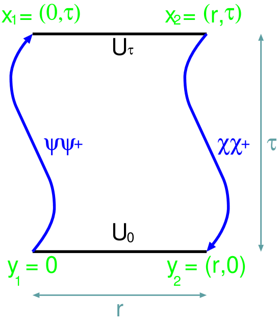
Figure 6.5: The four point function of Eq. (6.28).

We can now combine two such propagators into a generalised (fluctuating) rectangular Wilson loop,

$$G_{i^{\prime}j^{\prime}ij}(r,\tau)=\left\langle\mbox{Tr}\left[U_{0}K_{i^{\prime}i}(y_{1},x_{1})U_{\tau}K_{j^{\prime}j}(x_{2},y_{2})\right]\right\rangle,$$ (6.28)

where the indices $i,j$ and $i^{\prime},j^{\prime}$ represent the spins of the initial and final states. Note that $G$, unlike the argument of the expectation value, is real in Euclidean space-time. For the case of quark and anti-quark having different masses, two different propagators, $K_{\psi}$ and $K_{\chi}$, must be used within the above formula. We denote the temporal extent by, $\tau=y_{1,4}-x_{1,4}=y_{2,4}-x_{2,4}$, and the spatial separation by ${\mathbf{r}}={\mathbf{y}}_{2}-{\mathbf{y}}_{1}={\mathbf{x}}_{2}-{\mathbf{x}}_{1}$. The situation is visualised in Figure 6.5. For the sake of simplicity, we switch to leading order NRQCD with equal quark masses. In this case,

$$H_{1}=m+igA_{4}+\frac{p^{2}}{2m_{\psi}}.$$ (6.29)

To lowest order in $v/c$, the exponent within Eq. (6.27) can be approximated by the value it takes along the shortest path [26, 27]. Thus,

$$G({\mathbf{r}},\tau)=\exp\left[\int_{0}^{\tau}\!dt\,\sum_{j=1}^{2}\left({\mathbf{p}}_{j}\dot{\mathbf{x}}_{j}-m-\frac{{\mathbf{p}}_{j}^{2}}{2m_{\psi}}\right)\right]\langle W({\mathbf{r}},\tau)\rangle.$$ (6.30)

In higher orders of the $v/c$ expansion fluctuations of the propagators around the classical paths have to be taken into account that result in additional terms. From the spectral decomposition of the Wilson loop,

$$\langle W({\mathbf{r}},\tau)\rangle\propto\exp[-V_{0}({\mathbf{r}})\tau]\quad(\tau\rightarrow\infty),$$ (6.31)

we arrive at,

$$-\frac{d}{dt}G=HG,$$ (6.32)

with

$$H=2m+\frac{p^{2}}{m}_{\psi}+V_{0}(r),$$ (6.33)

in the limit of large $\tau$: the result is a Schrödinger equation that governs the evolution of a quark anti-quark state in a gluonic background whose average effect is contained in the static potential, $V_{0}$. The validity of the instantaneous approximation is tied to that of the naïve quark model: if quarkonium states can be completely classified by the quantum numbers of the constituent quarks, then the spectrum and wave functions can be obtained by solving the quantum mechanical equation,

$$H\psi_{nll_{3}}({\mathbf{r}})=E_{nl}\psi_{nll_{3}}({\mathbf{r}}).$$ (6.34)

We have discussed above that $m$ will in general differ from the “kinetic” mass of the quark, $m_{\psi}=m(\mu)+\delta m(\mu)$. Furthermore, this difference will depend on the matching scale, $\mu$. In Section 4.5 we have also seen that the potential, $V_{0}(r,\mu)=\hat{V}_{0}(r)+V_{\mbox{\scriptsize self}}(\mu)$, can be factorised into a physical and a self-energy part. This observation results in the relation,

$$\delta m(\mu^{\prime})=\delta m(\mu)+\frac{1}{2}\left[V_{\mbox{\scriptsize self}}(\mu^{\prime})-V_{\mbox{\scriptsize self}}(\mu)\right],$$ (6.35)

i.e. $\delta m(\mu)$ diverges as $\mu\rightarrow\infty$.

In lattice NRQCD, it is straight forward to calculate masses of quarkonia states, $E_{\Upsilon}(p)$, projected onto non-vanishing momentum, $p$. We use the convention that $E_{\Upsilon}$ is the sum of the bare quark masses, $2m$, and the energy shift due to the interaction terms of the Hamiltonian. By requiring the correct dispersion relation to the given order of the expansion,

$$E_{\Upsilon}(p)-E_{\Upsilon}(0)=\frac{p^{2}}{2m_{\Upsilon}}-\frac{p^{4}}{8m_{\Upsilon}^{3}}\quad\left(\quad+\cdots\quad\right),$$ (6.36)

the $\Upsilon$ rest mass, $m_{\Upsilon}$, can be determined. The mass shift, then, is given by, $2\delta m=E_{\Upsilon}(0)-m_{\Upsilon}$. Within the potential approach, the zero point energy at first appears to be difficult to determine in a similar way. However, in principle it should be possible to calculate potentials governing finite momentum quarkonia states too, by starting the derivation from a boosted NRQCD Lagrangian.

6.3.2 Relativistic corrections

The Hamiltonian Eqs. (6.31) – (6.33) was first obtained in Ref. [175] in a systematic way from continuum QCD where the static Dirac equation, $\left(\gamma_{4}D_{4}+m\right)q=0$, is solved by a Schwinger line times a factor, $e^{-mt}$, after projecting onto quark and anti-quark states. Starting from QCD, Eichten, Feinberg and Gromes derived spin dependent correction terms [22, 23, 25] (see also the article by Peskin [24]). Finally, Brambilla and collaborators (BBP) [26, 27] found an additional relativistic correction term to the central potential that had previously been ignored and added further velocity (or momentum) dependent terms by taking fluctuations of the heavy quark propagators into account. In general, apart from the one-particle Lagrangians, ${\mathcal{L}}_{i},i=\psi,\chi$, [Eqs. (6.6) – (6.1.2)] the two-particle Greens function receives contact term contributions from the two-particle sector Lagrangian of Eq. (6.1.2) [28], ${\mathcal{L}}_{\psi\chi}$. Taking these into account too, the complete result to this order in $c^{-1}$, with the NRQCD matching coefficients included [28, 29, 398], in the centre of mass frame (${\mathbf{p}}={\mathbf{p}_{1}}=-{\mathbf{p}_{2}}$ and ${\mathbf{L}}={\mathbf{L}_{1}}={\mathbf{L}_{2}}$), for $m_{1}\geq m_{2}$ is,

$$H = \sum_{i=1}^{2}\left(m_{i}-\delta m_{i}+\frac{p^{2}}{2m_{i}}-\frac{p^{4}}{8m_{i}^{3}}\right)$$ (6.37)

$$+ V(r,{\mathbf{p}},{\mathbf{L}},{\mathbf{S}_{1}},{\mathbf{S}_{2}}),$$

where the potential,

$$V(r,{\mathbf{p}},{\mathbf{L}},{\mathbf{S}_{1}},{\mathbf{S}_{2}})=V_{0}(r)+V_{\mbox{\scriptsize C}}+V_{\mbox{\scriptsize SD}}(r,{\mathbf{L}},{\mathbf{S}_{1}},{\mathbf{S}_{2}})+V_{\mbox{\scriptsize MD}}(r,{\mathbf{p}}),$$ (6.38)

contains corrections to the central potential (C) as well as spin dependent (SD) and momentum dependent (MD) corrections. $V_{0}(r)$ denotes the static potential while,

$$V_{\mbox{\scriptsize C}}(r) = \frac{d_{s}}{m_{1}m_{2}}4\pi C_{F}\alpha_{s}\delta^{3}({\mathbf{r}})$$

$$+ \sum_{i=1}^{2}\frac{1}{8m_{i}^{2}}\left\{c_{D}^{(i)}\left[\nabla^{2}V_{0}(r)+\nabla^{2}V_{a}^{E}(r)\right]+{c_{F}^{(i)}}^{2}\nabla^{2}V_{a}^{B}(r)\right\}$$

$$+ \left(\frac{1}{m_{1}}+\frac{1}{m_{2}}\right)V_{\prime}(r),$$

$$V_{\mbox{\scriptsize SD}}(r,{\mathbf{L}},{\mathbf{S}_{1}},{\mathbf{S}_{2}}) = \left(\frac{{\mathbf{S}_{1}}}{m_{1}^{2}}+\frac{{\mathbf{S}_{2}}}{m_{2}^{2}}\right){\mathbf{L}}\frac{(2c_{+}-1)V_{0}^{\prime}(r)+2c_{+}V_{1}^{\prime}(r)}{2r}$$

$$+ \frac{{\mathbf{S}_{1}}+{\mathbf{S}_{2}}}{m_{1}m_{2}}{\mathbf{L}}\frac{c_{+}V_{2}^{\prime}(r)}{r}$$

$$+ \left(\frac{{\mathbf{S}_{1}}}{m_{1}^{2}}-\frac{{\mathbf{S}_{2}}}{m_{2}^{2}}\right){\mathbf{L}}\frac{c_{-}[V_{0}^{\prime}(r)+V_{1}^{\prime}(r)]}{r}$$

$$+ \frac{{\mathbf{S}_{1}}-{\mathbf{S}_{2}}}{m_{1}m_{2}}{\mathbf{L}}\frac{c_{-}V_{2}^{\prime}(r)}{r}$$

$$+ \frac{S_{1}^{i}S_{2}^{j}}{m_{1}m_{2}}c_{F}^{(1)}c_{F}^{(2)}R_{ij}V_{3}(r)$$

$$+ \frac{{\mathbf{S}_{1}}\cdot{\mathbf{S}_{2}}}{3m_{1}m_{2}}\left[c_{F}^{(1)}c_{F}^{(2)}V_{4}(r)-12d_{v}4\pi C_{F}\alpha_{s}\delta^{3}({\mathbf{r}})\right],$$

and

$$V_{\mbox{\scriptsize MD}}(r,{\mathbf{p}}) = -\frac{1}{m_{1}m_{2}}\left\{p_{i},p_{j},[\delta_{ij}V_{b}(r)-R_{ij}V_{c}(r)]\right\}_{\mbox{\scriptsize Weyl}}$$

$$+ \sum_{k=1}^{2}\frac{1}{m_{k}^{2}}\left\{p_{i},p_{j},[\delta_{ij}V_{d}(r)-R_{ij}V_{e}(r)]\right\}_{\mbox{\scriptsize Weyl}},$$

with

$$R_{ij} = \frac{r_{i}r_{j}}{r^{2}}-\frac{\delta_{ij}}{3},$$ (6.42)

$$\delta m_{i} = \delta m(m_{i},\mu),$$ (6.43)

$$c_{F,D}^{(i)} = c_{F,D}(m_{i},\mu),$$ (6.44)

$$c_{\pm} = c_{\pm}(m_{1},m_{2},\mu)=\frac{1}{2}\left(c_{F}^{(1)}\pm c_{F}^{(2)}\right),$$ (6.45)

$$d_{s} = \frac{1}{4\pi C_{F}\alpha_{s}}\left[d_{ss}(m_{1},m_{2},\mu)+C_{F}d_{vs}(m_{1},m_{2},\mu)\right],$$ (6.46)

$$d_{v} = \frac{1}{4\pi C_{F}\alpha_{s}}\left[d_{sv}(m_{1},m_{2},\mu)+C_{F}d_{vv}(m_{1},m_{2},\mu)\right].$$ (6.47)

The symbol $\{a,b,c\}_{\mbox{\scriptsize Weyl}}=\frac{1}{4}\{a,\{b,c\}\}$ denotes Weyl ordering of the three arguments. Note that in the equal mass case, that has been considered in Ref. [23], where $c_{-}$ assumes its tree level value, $c_{-}=0$, two of the spin-orbit terms vanish. The term proportional to $V_{\prime}$ in Eq. (6.3.2) has been identified very recently [32] and in principle additional $1/m^{2}$ corrections to $V_{\mbox{\scriptsize C}}$ should exist [32], albeit to higher order in the $c^{-1}$ power counting than order $c^{-2}$ considered above.

The last term of Eq. (6.3.2) has been written in a somewhat suggestive way that is motivated by the expectation, $V_{4}(r)\approx 8\pi C_{F}\alpha_{s}\delta^{3}({\mathbf{r}})$. $c_{S}$ has been eliminated from the above formulae by using the re-parametrisation invariance relation, Eq. (6.15). Note that neither $d_{vv}^{c}$ or $d_{vs}^{c}$ nor $d_{ss}$ or $d_{sv}$ contribute to $d_{s}$ or $d_{v}$. This means that even in the equal mass case, where $d_{vv}^{c}=-\pi\alpha_{s}+\cdots$, $d_{s}$ and $d_{v}$ are of order $\alpha_{s}$. The one loop results in the $\overline{MS}$ scheme are displayed in Eqs. (E.22) and (E.23) of Appendix E.

$V_{0}$, $V_{\prime}$, $\nabla^{2}V_{a}^{E}$, $\nabla^{2}V_{a}^{B}$, $V_{1}^{\prime},\ldots,V_{4}$ and $V_{b},\ldots,V_{e}$ can be computed from lattice correlation functions (in Euclidean time) of Wilson loop like operators. The functions $V_{1}^{\prime},\ldots,V_{4}$ are related to spin-orbit and spin-spin interactions. The MD potential gives rise to correction terms of the form $\frac{1}{r}{\mathbf{L}}^{2}$, $\frac{1}{r^{3}}{\mathbf{L}}^{2}$, $\frac{1}{r}p^{2}$, $\frac{1}{r}$ and $\delta^{3}(r)$, and the correction to the central potential includes the expected Darwin term, $\nabla^{2}V_{0}$, as well as $\nabla^{2}V_{a}^{E}$ and $\nabla^{2}V_{a}^{B}$.

6.3.3 Scale dependence

The SD potentials, $V_{1}^{\prime},\ldots,V_{4}$, as well as $\nabla^{2}V_{a}^{E}$ and $\nabla^{2}V_{a}^{B}$ depend on the matching scale, $\mu$. The potentials $V_{0}$, $V_{\prime}$ as well as $V_{b},\ldots,V_{e}$ can contain additive, $\mu$ dependent self energy contributions; however, their derivatives are scale independent.

Due to Lorentz invariance, certain pairs of potentials are related to the static potential by the Gromes [399] and BBP [27] relations,

$$V_{2}^{\prime}(\mu;r)-V_{1}^{\prime}(\mu;r) = V_{0}^{\prime}(r),$$ (6.48)

$$V_{b}(r;\mu)+2V_{d}(r;\mu) = \frac{r}{6}V_{0}^{\prime}(r)-\frac{1}{2}V_{0}(r;\mu),$$ (6.49)

$$V_{c}(r)+2V_{e}(r) = -\frac{r}{2}V_{0}^{\prime}(r),$$ (6.50)

such that three potentials, e.g. $V_{2}^{\prime}$, $V_{d}$ and $V_{e}$ can be eliminated from the Hamiltonian. Note that Eq. (6.48) implies Eq. (6.15). Given the structure of the Hamiltonian, Eqs. (6.37) – (6.3.2), and the Gromes relation, Eq. (6.48), we can deduce [400, 29] the following relations between potentials, evaluated at cut-off scales $\mu$ and $\mu^{\prime}$, by demanding $dH/d\ln\mu=0$,

$$\nabla^{2}V_{a}^{E}(\mu^{\prime};r) = \frac{1}{c_{D}(\mu^{\prime})}\left\{c_{D}(\mu)\nabla^{2}V_{a}^{E}(\mu;r)+[c_{D}(\mu)-c_{D}(\mu^{\prime})]\nabla^{2}V_{0}(r)\right.$$ (6.51)

$$+ \left.c_{F}^{2}(\mu)\nabla^{2}V_{a}^{B}(\mu;r)+c_{F}^{2}(\mu^{\prime})\nabla^{2}V_{a}^{B}(\mu^{\prime};r)\right\},$$

$$V_{1}^{\prime}(\mu^{\prime};r) = V_{1}^{\prime}(\mu;r)-\left[1-\frac{c_{F}(\mu^{\prime})}{c_{F}(\mu)}\right]V_{2}^{\prime}(\mu;r),$$ (6.52)

$$V_{2}^{\prime}(\mu^{\prime};r) = \frac{c_{F}(\mu)}{c_{F}(\mu^{\prime})}V_{2}^{\prime}(\mu;r),$$ (6.53)

$$V_{3}(\mu^{\prime};r) = \frac{c_{F}^{2}(\mu)}{c_{F}^{2}(\mu^{\prime})}V_{3}(\mu;r),$$ (6.54)

$$V_{4}(\mu^{\prime};r) = \frac{1}{c_{F}^{2}(\mu^{\prime})}\left\{c_{F}^{2}(\mu)V_{4}(\mu;r)\right.$$ (6.55)

$$- \left.12[d_{v}(\mu)-d_{v}(\mu^{\prime})]4\pi C_{F}\alpha_{s}\delta^{3}({\mathbf{r}})\right\}.$$

Since the potentials, appearing in the above relations, do not depend on the quark mass, the ratios $c_{F,D}(m,\mu)/c_{F,D}(m,\mu^{\prime})$ must not depend on $m$. Therefore, the matching coefficients can always be factorised into two separate functions, $c_{i}(m,\mu)=f_{i}(m)g_{i}^{-1}(\mu)$.

6.3.4 Integrating out gluons

We have managed to separate the time dependence of the interaction into coefficient functions of various interaction terms, $V_{i}$, which we shall call the potentials. These potentials can be computed as expectation values in presence of a gauge field background [23, 26, 401, 29],

$$\nabla^{2}{V}_{a}^{E}({\mathbf{r}}) = 2\,g^{2}\lim\limits_{\tau\to\infty}\int_{0}^{\tau}\!dt\,\langle\langle{\mathbf{E}}({\mathbf{0}},0)\cdot{\mathbf{E}}({\mathbf{0}},t)\rangle\rangle_{W}^{c},$$ (6.56)

$$\nabla^{2}{V}_{a}^{B}({\mathbf{r}}) = 2\,g^{2}\lim\limits_{\tau\to\infty}\int_{0}^{\tau}\!dt\,\langle\langle{\mathbf{B}}({\mathbf{0}},0)\cdot{\mathbf{B}}({\mathbf{0}},t)\rangle\rangle_{W},$$ (6.57)

$$V_{\prime}({\mathbf{r}}) = -\frac{g^{2}}{2}\lim\limits_{\tau\to\infty}\int_{0}^{\tau}\!dt\,t\,\langle\langle{\mathbf{E}}({\mathbf{0}},0)\cdot{\mathbf{E}}({\mathbf{0}},t)\rangle\rangle_{W}^{c},$$ (6.58)

where the superscript “$c$” denotes the connected part,

$$\langle\langle AB\rangle\rangle_{W}^{c}=\langle\langle AB\rangle\rangle_{W}-\langle\langle A\rangle\rangle_{W}\langle\langle B\rangle\rangle_{W}.$$ (6.59)

For the SD potentials one finds,

$$\frac{r_{k}}{r}{V}_{1}^{\prime}({\mathbf{r}}) = \epsilon_{ijk}g^{2}\lim\limits_{\tau\to\infty}\!\int_{0}^{\tau}\!\!dt\,t\langle\langle{B}_{i}({\mathbf{0}},0){E}_{j}({\mathbf{0}},t)\rangle\rangle_{W},$$ (6.60)

$$\frac{r_{k}}{r}{V}_{2}^{\prime}({\mathbf{r}}) = \frac{1}{2}\epsilon_{ijk}g^{2}\lim\limits_{\tau\to\infty}\!\int_{0}^{\tau}\!dt\,t\langle\langle{B}_{i}({\mathbf{0}},0){E}_{j}({\mathbf{r}},t)\rangle\rangle_{W},$$ (6.61)

$$R_{ij}V_{3}({\mathbf{R}}) = 2\,g^{2}\lim\limits_{\tau\to\infty}\int_{0}^{\tau}\!dt\,\left[\langle\langle{B}_{i}({\mathbf{0}},0){B}_{j}({\mathbf{r}},t)\rangle\rangle_{W}\right.$$

$$- \frac{\delta_{ij}}{3}\left.\langle\langle{\mathbf{B}}({\mathbf{0}},0)\cdot{\mathbf{B}}({\mathbf{r}},t)\rangle\rangle_{W}\right],$$

$${V}_{4}({\mathbf{R}}) = 2\,g^{2}\lim\limits_{\tau\to\infty}\int_{0}^{\tau}\!dt\,\langle\langle{\mathbf{B}}({\mathbf{0}},0)\cdot{\mathbf{B}}({\mathbf{r}},t)\rangle\rangle_{W},$$ (6.63)

where $R_{ij}$ is defined in Eq. (6.42). Finally, the MD potentials are,

$${V}_{b}({\mathbf{r}}) = -\frac{1}{3}g^{2}\,\lim\limits_{\tau\to\infty}\int_{0}^{\tau}\!dt\,t^{2}\langle\langle{\mathbf{E}}({\mathbf{0}},0)\cdot{\mathbf{E}}({\mathbf{r}},t)\rangle\rangle_{W}^{c},$$ (6.64)

$$R_{ij}{V}_{c}({\mathbf{r}}) = g^{2}\lim\limits_{\tau\to\infty}\int_{0}^{\tau}\!dt\,t^{2}\left[\langle\langle{E}_{i}({\mathbf{0}},0){E}_{j}({\mathbf{r}},t)\rangle\rangle_{W}^{c}\right.$$

$$- \frac{\delta_{ij}}{3}\left.\langle\langle{\mathbf{E}}({\mathbf{0}},0)\cdot{\mathbf{E}}({\mathbf{r}},t)\rangle\rangle_{W}^{c}\right],$$

$${V}_{d}({\mathbf{r}}) = \frac{1}{6}g^{2}\lim\limits_{\tau\to\infty}\int_{0}^{\tau}\!dt\,t^{2}\langle\langle{\mathbf{E}}({\mathbf{0}},0)\cdot{\mathbf{E}}({\mathbf{0}},t)\rangle\rangle_{W}^{c},$$ (6.66)

$$R_{ij}{V}_{e}({\mathbf{r}}) = -\frac{1}{2}g^{2}\lim\limits_{\tau\to\infty}\int_{0}^{\tau}\!dt\,t^{2}\left[\langle\langle{E}_{i}({\mathbf{0}},0){E}_{j}({\mathbf{0}},t)\rangle\rangle_{W}^{c}\right.$$

$$- \frac{\delta_{ij}}{3}\left.\langle\langle{\mathbf{E}}({\mathbf{0}},0)\cdot{\mathbf{E}}({\mathbf{0}},t)\rangle\rangle_{W}^{c}\right].$$

While $V_{0},V_{b},\ldots,V_{e}$ have the dimension $m$, $V_{\prime}$, $V_{1}^{\prime}$ and $V_{2}^{\prime}$ have dimension $m^{2}$ and $V_{3}$, $V_{4}$, $\nabla^{2}V_{a}^{E}$ and $\nabla^{2}V_{a}^{B}$ have dimension $m^{3}$.

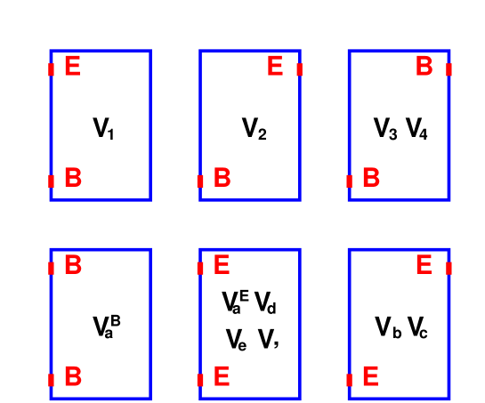
Figure 6.6: The nominators of the arguments of the integrals within Eqs. (6.56) – (6.3.4).

Throughout the previous equations, the expectation value, $\langle\langle F_{1}F_{2}\rangle\rangle_{W}$, is defined as,

$$\left\langle\langle F_{1}F_{2}\rangle\right\rangle_{W(C)}=\frac{\langle\mbox{Tr}\,{\mathcal{P}}\left[\exp\left(ig\int_{\delta C}dx_{\mu}\,A_{\mu}\right)F_{1}F_{2}\right]\rangle}{\langle\mbox{Tr}\,{\mathcal{P}}\left[\exp\left(ig\int_{\delta C}dx_{\mu}\,A_{\mu}\right)\right]\rangle},$$ (6.68)

where $\delta C$ represents a closed path [the contour of a Wilson loop, $W({\mathbf{r}},T)$, $T\geq\tau$]. The nominators of Eq. (6.68) that are required to compute the potentials are depicted in Figure 6.6. The correlators appearing within the coefficient functions of the spin-orbit potentials, $V_{1}^{\prime}$ and $V_{2}^{\prime}$, involve electric and magnetic fields, the latter originating from the angular movement. Correlators between two magnetic fields are required in the spin-spin potentials, $V_{3}$ and $V_{4}$, which arise from interactions between the two Fermi terms $\propto g\,{\mathbf{S}_{i}}\cdot{\mathbf{B}}/m_{i}$. The corrections to the central potential, $\nabla^{2}V_{a}^{E}$ and $\nabla^{2}V_{a}^{B}$, involve electric-electric and magnetic-magnetic interactions, respectively, while $V_{\prime}$ and all MD corrections involve two electric field insertions. The latter arise from re-expressing derivatives acting on the static propagators in terms of field strength insertions.

In principle similar results that would include Wilson loops with more than two field strength insertions can be obtained from the order $c^{-4}$ (or $v^{6}$) NRQCD Lagrangian of Ref. [35]. This tedious work has not been done yet since the dominant sources of error at present are the uncertainties of the matching coefficients and certain transition matrix elements (cf. Sections 7.2, 6.5.2 and 6.5.4), rather than higher order relativistic corrections.

6.3.5 The potentials as perturbations

In Refs. [401, 29] spectral decompositions of the above potentials have been derived. The results can be written as follows,

$$V_{3,4}(r) = \sum_{n>0}D_{n}^{(3,4)}(r)\int_{0}^{\tau}dt\,e^{-\Delta V_{n}(r)t}=\sum_{n>0}\frac{D_{n}^{(3,4)}(r)}{\Delta V_{n}(r)},$$ (6.69)

$$\nabla^{2}V_{a}^{E,B}(r) = \sum_{n>0}D_{n}^{(E,B)}(r)\int_{0}^{\tau}dt\,e^{-\Delta V_{n}(r)t}=\sum_{n>0}\frac{D_{n}^{(E,B)}(r)}{\Delta V_{n}(r)},$$ (6.70)

$$V^{\prime}_{1,2}(r) = \sum_{n>0}D_{n}^{(1,2)}(r)\int_{0}^{\tau}dt\,t\,e^{-\Delta V_{n}(r)t}=\sum_{n>0}\frac{D_{n}^{(1,2)}(r)}{[\Delta V_{n}(r)]^{2}},$$ (6.71)

$$V_{\prime}(r) = \sum_{n>0}D_{n}^{\prime}(r)\int_{0}^{\tau}dt\,t\,e^{-\Delta V_{n}(r)t}=\sum_{n>0}\frac{D_{n}^{\prime}(r)}{[\Delta V_{n}(r)]^{2}},$$ (6.72)

$$V_{b,c,d,e}(r) = \sum_{n>0}D_{n}^{(b,c,d,e)}(r)\int_{0}^{\tau}dt\,\frac{t^{2}}{2}\,e^{-\Delta V_{n}(r)t}=\sum_{n>0}\frac{D_{n}^{(b,c,d,e)}(r)}{[\Delta V_{n}(r)]^{3}},$$ (6.73)

where $\Delta V_{n}(r)=V_{n}(r)-V_{0}(r)$ denotes the difference between the $n$th hybrid excitation and the ground state $\Sigma_{g}^{+}$ potential. The coefficients, $D_{n}(r)$, are real parts of products of two transition amplitudes and can easily be read off from Eqs. (6.56) – (6.3.4). For instance, in the case of $V_{4}$, one obtains,

$$D_{n}^{4}(r)=2\,g^{2}\mbox{Re}\,\left[\langle\Phi_{{\mathbf{r}},0}|{\mathbf{B}}({\mathbf{0}})|\Phi_{{\mathbf{r}},n}\rangle\langle\Phi_{{\mathbf{r}},n}|{\mathbf{B}}({\mathbf{r}})|\Phi_{{\mathbf{r}},0}\rangle\right],$$ (6.74)

where $|\Phi_{{\mathbf{r}},n}\rangle$ denotes the $n$th excitation of a quark anti-quark state at separation, ${\mathbf{r}}$, and the states are thought to be normalised, $\langle\Phi_{{\mathbf{r}},i}|\Phi_{{\mathbf{r}},i}\rangle=1$. Note that, $D_{n}^{E}=-4D_{n}^{\prime}=6D_{n}^{d}$.

Physically, the above result can be interpreted as follows [402, 401]: at time $0$ the spin of the quark at position, ${\mathbf{0}}$, interacts with the background glue and excites the gluonic vortex until, at time $\tau$ a second interaction with the spin of the anti-quark at ${\mathbf{r}}$ takes place that returns the flux tube into its ground state: the non-perturbative analogue of a gluon exchange! From Table 5.1 one can read off that in general the intermediate state will be a superposition of excitations within the $\Sigma_{u}^{-}$ and $\Pi_{u}$ channels in the particular cases of $V_{3},V_{4}$ and $\nabla^{2}V_{a}^{B}$.

We add the term proportional to $\nabla^{2}V^{B}_{a}$ of Eq. (6.3.2) to the two terms proportional to $V_{3}$ and $V_{4}$ of Eq. (6.3.2). The result reads,

$$V_{\mbox{\scriptsize ss}}(r) = c_{F}^{(1)}c_{F}^{(2)}\frac{S_{1}^{i}S_{2}^{j}}{3m_{1}m_{2}}\left[3R_{ij}V_{3}(r)+\delta_{ij}V_{4}(r)\right]$$

$$+ \left(\frac{{c_{F}^{(1)}}^{2}}{8m_{1}^{2}}+\frac{{c_{F}^{(2)}}^{2}}{8m_{2}^{2}}\right)\nabla^{2}V_{a}^{B}(r).$$

By inserting the spectral decomposition with the correct coefficients, $D_{n}$, determined from Eqs. (6.57), (6.3.4) and (6.63), into Eq. (6.3.5) one obtains,

$$V_{\mbox{\scriptsize ss}}(r) = \sum_{n>0}\frac{1}{V_{n}(r)-V_{0}(r)}$$

$$\times \left|\left\langle\Phi_{{\mathbf{r}},0}\left|\left[c_{F}^{(1)}\frac{g{\mathbf{S}}_{1}\cdot{\mathbf{B}}({\mathbf{0}})}{m_{1}}+c_{F}^{(2)}\frac{g{\mathbf{S}_{2}}\cdot{\mathbf{B}}({\mathbf{r}})}{m_{2}}\right]\right|\Phi_{{\mathbf{r}},n}\right\rangle\right|^{2},$$

where we have exploited the fact that ${\mathbf{B}}^{2}=4({\mathbf{S}}\cdot{\mathbf{B}})^{2}$. The result is exactly the energy shift one would have expected in second order perturbation theory from the Fermi terms for quark and anti-quark within Eq. (6.1.2),

$$V_{\mbox{\scriptsize ss}}(r)=\Delta E_{\mbox{\scriptsize ss}}=\sum_{n>0}\frac{\langle\Phi_{{\mathbf{r}},0}|\Delta H_{\mbox{\scriptsize ss}}|\Phi_{{\mathbf{r}},n}\rangle\langle\Phi_{{\mathbf{r}},n}|\Delta H_{\mbox{\scriptsize ss}}|\Phi_{{\mathbf{r}},0}\rangle}{V_{n}(r)-V_{0}(r)},$$ (6.77)

with

$$\Delta H_{\mbox{\scriptsize ss}}({\mathbf{x}})=\frac{c_{F}^{(1)}g{\mathbf{\sigma}_{1}}\cdot{\mathbf{B}}({\mathbf{x}})}{2m_{1}}\delta^{3}({\mathbf{x}})+\frac{c_{F}^{(2)}g{\mathbf{\sigma}_{2}}\cdot{\mathbf{B}}({\mathbf{x}})}{2m_{2}}\delta^{3}({\mathbf{x}}-{\mathbf{r}}),$$ (6.78)

where ${\mathbf{\sigma}}_{i}=2{\mathbf{S}}_{i}$.

Other potentials in their spectral representation can be interpreted as perturbations too. However, relating these to the NRQCD Lagrangian requires somewhat more involved formal manipulations. From the considerations above it is obvious that the formalism cannot readily be applied to spin dependent interactions of hybrid quarkonia where the $\Sigma^{+}_{g}$ ground state would appear as an intermediate state: since $\exp[-(V_{n}-V_{m})t]$ diverges with $t$ for $m>n$; the matrix elements corresponding to Eq. (6.77), for an external state, $|\Phi_{{\mathbf{r}},m}\rangle$, cannot be obtained from a simple time integral over double bracket expectation values.

6.4 Model expectations

We discuss expectations for the potentials and the resulting Hamiltonian, and discuss the Lorentz structure of the effective interaction kernel.

6.4.1 The potentials

We will present simple model expectations for the above potentials. The double bracket expectation values of colour field operators can be obtained from infinitesimal deformations of a generalised, non-static Wilson loop [358],

$$g^{2}\langle F_{\mu\nu}(x)F_{\rho\sigma}(y)\rangle\rangle^{c}_{W}=-\frac{\delta^{2}\ln\langle W\rangle}{\delta S_{\mu\nu}(x)\delta S_{\rho\sigma}(y)}.$$ (6.79)

If the functional dependence of the Wilson loop expectation value on its contour is known, the above formula can be applied to calculate the corresponding long distance behaviour of the potentials. This has been done for the stochastic vacuum model (SVM), dual QCD and the area law assumption in Refs. [60, 61]. A variety of predictions on SD and MD potentials exists in the literature that are based on effective modified one gluon exchanges or Bethe Salpeter kernels. Ref. [403] represents a recent example. Given these different suggestions, lattice results with a precision that is sufficient to discriminate between them are highly desirable.

Here, we shall only discuss the area law expectations [26, 27], combined with tree level perturbation theory and constraints from the renormalisation group mixing between the potentials [29], Eqs. (6.51) – (6.55),

$$V_{0}(r;\mu) = V_{\mbox{\scriptsize self}}(\mu)-\frac{e}{r}+\sigma r,$$ (6.80)

$$\nabla^{2}V_{a}^{E}(r;\mu) = C_{a}^{E}(\mu)-\frac{2\sigma+b(\mu)}{r},$$ (6.81)

$$\nabla^{2}V_{a}^{B}(r;\mu) = C_{a}^{B}(\mu),$$ (6.82)

$$V_{1}^{\prime}(r;\mu) = -\frac{h(\mu)}{r^{2}}-\sigma,$$ (6.83)

$$V_{2}^{\prime}(r;\mu) = \frac{e-h(\mu)}{r^{2}},$$ (6.84)

$$V_{3}(r;\mu) = 3\frac{e-h(\mu)}{r^{3}},$$ (6.85)

$$V_{4}(r;\mu) = 8\pi[e-h(\mu)]\delta^{3}(r),$$ (6.86)

$$V_{\prime}(r) = 0,$$ (6.87)

$$V_{b}(r;\mu) = C_{b}(\mu)+\frac{2}{3}\frac{e}{r}-\frac{\sigma}{9}r,$$ (6.88)

$$V_{c}(r) = -\frac{1}{2}\frac{e}{r}-\frac{\sigma}{6}r,$$ (6.89)

$$V_{d}(r;\mu) = C_{d}(\mu)-\frac{\sigma}{9}r,$$ (6.90)

$$V_{e}(r) = -\frac{\sigma}{6}r,$$ (6.91)

with $e-h(\mu)\approx C_{F}\alpha_{s}$. The above formulae conform with the Gromes and BBP relations, Eqs. (6.48) – (6.50). While $V_{0}$, $V_{\prime}$ and the MD potentials do not undergo multiplicative renormalisation, $V_{0}$, $V_{b}$ and $V_{d}$ still contain additive self-energy contributions that will diverge as $\mu\rightarrow\infty$ and whose $\mu$ dependence has to be cancelled by the quark mass shifts, $\delta m_{i}$. The constants, $V_{\mbox{\scriptsize self}}(\mu)$, $C_{a}^{E}(\mu)$, $C_{a}^{B}(\mu)$, $C_{b}(\mu)$ and $C_{d}(\mu)$ as well as all terms proportional to $e$ originate from perturbation theory, while all terms proportional to the string tension, $\sigma$, are due to the area law ansatz, with the exception of $\nabla^{2}V_{a}^{E}$. We allow for terms proportional to $h$ in $V_{1}^{\prime}$ and $V_{2}^{\prime}$ that are thought to originate from the mixing between these two potentials under renormalisation group transformations, Eq. (6.52). In perturbation theory as well as in vector exchange models, one obtains, $V_{3}(r)=V_{2}^{\prime}/r-V_{2}^{\prime\prime}$ and $V_{4}=2\nabla^{2}V_{2}$. Therefore, replacing $C_{F}\alpha_{s}$ by $e-h$ within these potentials appears to be reasonable. However, we remark that further corrections to this ansatz must exist since the scaling behaviours under $\mu\rightarrow\mu^{\prime}$ of $V_{2}$ [Eq. (6.53)], $V_{3}$ [Eq. (6.54)] and $V_{4}$ [Eq. (6.55)] are incompatible with each other. Finally, the expectation, $2\sigma+b(\mu)$, within $\nabla^{2}V_{a}^{E}$ is motivated by the lattice results to be presented in Section 6.6 as well as by dual QCD and SVM calculations [60, 61]. One would expect additional $\delta$-like contributions to $\nabla^{2}V_{a}^{E}$ and $\nabla^{2}V_{a}^{B}$ from Eq. (6.51), which we ignore for the moment.

Interestingly, by adding a perimeter term to the Wilson loop area law [26, 27], one obtains a non-vanishing $C_{d}=-V_{\mbox{\scriptsize self}}/4$, which agrees with the expectation from perturbation theory. However, the perimeter term does not contribute to $C_{a}^{E}$, $C_{a}^{B}$ or $C_{b}$. In continuum perturbation theory as well as in lattice perturbation theory in the infinite volume limit, one obtains the tree level results [29],

$$C_{b}(\mu)=0,\quad C_{d}(\mu)=-\frac{1}{4}V_{\mbox{\scriptsize self}}(\mu),$$ (6.92)

where the lattice perturbation theory result for $V_{\mbox{\scriptsize self}}(a)$ with the Wilson action is given in Eq. (4.53). By using the lattice field definitions of Eqs. (5.3) – (5.6), we obtain the lattice perturbation theory results [29],

$$C_{a}^{E}(a) = -C_{F}\alpha_{s}a^{-3}\times 7.91084\ldots,$$ (6.93)

$$C_{a}^{B}(a) = C_{F}\alpha_{s}a^{-3}\times 14.89413\ldots,$$ (6.94)

for the other two self-energy contributions.

6.4.2 The Hamiltonian

The Hamiltonian that results from the ansatz Eqs. (6.80) – (6.91), in the equal mass case, $m=m_{1}=m_{2}$, takes the form,

$$H = H_{0}+\delta H_{\mbox{\scriptsize kin}}+\frac{1}{m^{2}}\left(\delta H_{\delta}+\delta H_{\mbox{\scriptsize MD}}+\delta H_{\mbox{\scriptsize SD}}\right),$$ (6.95)

$$H_{0} = 2(m-\delta m)+V_{\mbox{\scriptsize self}}+\frac{1}{4m^{2}}\left(c_{D}C_{a}^{E}+c_{F}^{2}C_{a}^{B}\right)$$

$$+ \left[1-\frac{1}{2m}\left(V_{\mbox{\scriptsize self}}+4C_{b}\right)\right]\frac{p^{2}}{m}$$

$$- \left[e+\frac{3c_{D}b+2\sigma}{12m^{2}}\right]\frac{1}{r}+\sigma r,$$

$$\delta H_{\mbox{\scriptsize kin}} = -\frac{p^{4}}{4m^{3}},$$ (6.97)

$$\delta H_{\delta} = \left(\frac{3}{4}+d_{s}\right)4\pi e\delta^{3}({\mathbf{r}}),$$ (6.98)

$$\delta H_{\mbox{\scriptsize MD}} = -\frac{\sigma}{6r}{\mathbf{L}}^{2}-\frac{e}{r}\left(p^{2}-\frac{{\mathbf{L}}^{2}}{2r^{2}}\right),$$ (6.99)

$$\delta H_{\mbox{\scriptsize SD}} = \left[-\frac{\sigma}{r}+\frac{4c_{F}(e-h)-e}{r^{3}}\right]\frac{{\mathbf{L}}\cdot{\mathbf{S}}}{2}$$ (6.100)

$$+ \frac{3c_{F}^{2}(e-h)}{r^{3}}T+\left[2c_{F}^{2}(e-h)-12d_{v}e\right]4\pi\delta^{3}({\mathbf{r}})\frac{{\mathbf{S}}_{1}\cdot{\mathbf{S}}_{2}}{3},$$

with

$${\mathbf{L}}^{2} = l(l+1)$$ (6.101)

$$\frac{{\mathbf{S}}_{1}\cdot{\mathbf{S}}_{2}}{3} = \frac{1}{6}\left[s(s+1)-\frac{3}{2}\right],$$ (6.102)

$${\mathbf{L}}\cdot{\mathbf{S}} = \frac{1}{2}\left[J(J+1)-l(l+1)-s(s+1)\right],$$ (6.103)

$$T = R_{ij}S_{1}^{i}S_{2}^{j}=-\frac{6({\mathbf{L}}\cdot{\mathbf{S}})^{2}+3{\mathbf{L}}\cdot{\mathbf{S}}-2s(s+1)l(l+1)}{6(2l-1)(2l+3)}.$$ (6.104)

For a discussion of the non-equal mass case we refer the reader to Ref. [29]. The parametrisations of the potentials that enter the above Hamiltonian, can of course be improved in several ways, for example [398, 404] by including the known one loop perturbative results for the spin dependent terms [405, 367] and the two loop result for the static potential [260, 258]. Note that all terms containing the low-energy parameter, $\sigma$, are independent of the matching scale, $\mu\gg\sqrt{\sigma}$.

We have eliminated $C_{d}$ from the above Hamiltonian by use of Eq. (6.49), $V_{\mbox{\scriptsize self}}=-2C_{b}-4C_{d}$. The subscripts of the correction terms, $\delta H_{i}$, do not necessarily relate to the potentials of origin. $H_{0}$ contains contributions from $V_{0}$, $V_{\mbox{\scriptsize C}}$ as well as from $V_{\mbox{\scriptsize MD}}$ while $\delta H_{\delta}$ contains terms due to $V_{\mbox{\scriptsize C}}$ and $V_{\mbox{\scriptsize MD}}$. We have used the relation $2\pi\langle\delta^{3}({\mathbf{r}})\rangle=-i\langle r^{-3}{\mathbf{r}}\cdot{\mathbf{p}}\rangle$ to cast a term that appears within $V_{\mbox{\scriptsize MD}}$ into a $\delta$ function. The radial Schrödinger equation, Eq. (A.2), can be solved numerically for $H_{0}$ and, subsequently, the $\delta H_{i}$ terms can conveniently be treated as perturbations.

We substitute,

$$\tilde{m}=m+\frac{V_{\mbox{\scriptsize self}}+4C_{b}}{2}$$ (6.105)

into $H_{0}$. To order $m^{-2}$ this yields,

$$H_{0} = C_{0}+2\tilde{m}+\frac{p^{2}}{\tilde{m}}+\tilde{V}(r),$$ (6.106)

$$\tilde{V}(r) = -\frac{\tilde{e}}{r}+\sigma r,$$ (6.107)

$$C_{0} = -2\delta m-4C_{b}+\frac{1}{4{\tilde{m}}^{2}}\left(c_{D}C_{a}^{E}+c_{F}^{2}C_{a}^{B}\right),$$ (6.108)

$$\tilde{e} = e+\frac{3c_{D}b+2\sigma}{12\tilde{m}^{2}}:$$ (6.109)

the static quark self-energy shift, $V_{\mbox{\scriptsize self}}$, is eliminated from the Hamiltonian. This was first noticed in Ref. [27]. The remaining scale dependence of $\delta m(\mu)$ has to compensate that of the sum of the (small) term $C_{b}(\mu)$, which vanishes in tree level perturbation theory, and the term containing $C_{a}^{E}$ and $C_{a}^{B}$, which is suppressed by a factor $\tilde{m}^{-2}$. Moreover, $C_{a}^{E}$ and $C_{a}^{B}$ have different relative signs, such that partial cancellations occur. Of course, the above substitution is only valid for quark masses, $m\gg V_{\mbox{\scriptsize self}}\propto\alpha_{s}\mu$. This relation, however, is automatically fulfilled for matching scales, $\mu<m$. In conclusion: the mass shift, $\delta m$, which is related to the wave function renormalisation, becomes reduced as relativistic corrections are taken into account.

Some of the correction terms are well known from atomic physics, others are specific to non-Abelian gauge theories. One piece of $\delta H_{\delta}$ [Eq. (6.98)] as well as the term proportional to $b/r$ within Eq. (6.4.2) stem from the Darwin interaction. A string whose energy density, $\sigma$, is carried by a constant longitudinal electric field [42], gives rise to the (classical) orbit-orbit interaction term, $-\sigma/(6r){\mathbf{L}}^{2}$, that appears within Eq. (6.99). $\delta H_{\mbox{\scriptsize SD}}$ [Eq. (6.100)] contains a spin-orbit (Thomas) interaction term that, unlike its QED counterpart, only falls off like $r^{-1}$ at large distances. In addition, it contains two spin-spin interaction terms that take very much the same form as in QED, the first of which does not affect $S$ waves and the second of which only affects $S$ waves to the order in $\alpha_{s}$ considered above.

6.4.3 The Lorentz structure of the effective interaction

The general form of a Hamiltonian governing relativistic two-particle bound states has been derived within the Bethe-Salpeter formalism (see e.g. [227] and references therein), under the assumption that the interaction kernel only depends on the transfer momentum, $q^{2}$: The momentum space kernel can be decomposed into the five Lorentz invariants,

$$\tilde{I}=\tilde{V_{S}}\,{\mathbf{1}}\otimes{\mathbf{1}}+\tilde{V_{V}}\,\gamma_{\mu}\otimes\gamma_{\mu}+\tilde{V_{T}}\frac{1}{2}\sigma_{\mu\nu}\otimes\sigma_{\mu\nu}+\tilde{V_{A}}\,\gamma_{\mu}\gamma_{5}\otimes\gamma_{\mu}\gamma_{5}+\tilde{V_{P}}\,\gamma_{5}\otimes\gamma_{5},$$ (6.110)

where the form factors, $\tilde{V}_{i}$, only depend on $q^{2}$. In the QED case, within the ladder approximation, only $V_{V}$ assumes a non-trivial value and the resulting Hamiltonian has the Breit-Fermi form, well known from atomic physics. In the most general case [227] the equal mass Hamiltonian reads,

$$V(r) = V_{V}(r)+V_{S}(r)+4\left[V_{T}(r)-V_{A}(r)\right]{\mathbf{S}}_{1}\cdot{\mathbf{S}}_{2}$$

$$+ \frac{1}{m^{2}}\left\{\frac{1}{4}\nabla^{2}V_{V}(r)+\frac{{\mathbf{L}}\cdot{\mathbf{S}}}{2r}\left[3V_{V}^{\prime}(r)-V_{S}^{\prime}(r)\right]\right.$$

$$+ T\left[\frac{V_{V}^{\prime}(r)-V_{P}^{\prime}(r)}{r}+V_{P}^{\prime\prime}(r)-V_{V}^{\prime\prime}(r)\right]$$

$$+ \left.\frac{{\mathbf{S}}_{1}\cdot{\mathbf{S}}_{2}}{3}\left[2\nabla^{2}V_{V}(r)+\nabla^{2}V_{P}(r)\right]\right\},$$

where we have ignored momentum dependent terms as well as possible $m^{-2}$ corrections to $V_{A}(r)$ and $V_{T}(r)$.

Since QCD interactions are spin-independent to leading order, $V_{A}(r)=V_{T}(r)$ must be satisfied. Moreover, in comparing the above formula with the potential of Eqs. (6.38) – (6.3.2), with tree level matching constants, $c_{i}=1,d_{i}=0$, one finds,

$$V_{0} = V_{V}+V_{S},$$ (6.112)

$$V_{1} = -(1-\eta)V_{S},$$ (6.113)

$$V_{2} = V_{V}+\eta V_{S},$$ (6.114)

$$V_{3} = \frac{V_{V}^{\prime}-V_{P}^{\prime}}{r}-(V_{V}^{\prime\prime}-V_{P}^{\prime\prime}),$$ (6.115)

$$V_{4} = 2\nabla^{2}V_{V}+\nabla^{2}V_{P},$$ (6.116)

where we have also used the relation, Eq. (6.48). There are indications that the linear term, $\sigma\,r$, within $V_{0}$ should be purely scalar since vector type potentials are thought to rise at most logarithmically in $r$ [406]. The Darwin term appearing within Eq. (6.3.2) implies that $b=0$, i.e. any scalar contribution to $\nabla^{2}V_{0}$ has to be cancelled by the combination, $\nabla^{2}V_{a}^{E}+\nabla^{2}V_{a}^{B}$. It is clear that the picture becomes more involved when the matching coefficients assume non-trivial values. Moreover, the assumption that the interaction kernel only depends on the momentum transfer does not necessarily apply.

6.5 Beyond the adiabatic approximation

We shall briefly discuss the interrelation between local potentials, sum rules and the stochastic vacuum model. Following this, we shall describe pNRQCD which is a systematic and conceptionally attractive approach to quarkonia bound state problems. Subsequently, we will discuss some consequences that arise from including MD potentials. Finally, we incorporate hybrid states and transitions between different gluonic excitations of the string into the potential approach.

6.5.1 Are potentials enough?

The local potential picture of heavy quark bound states has often been challenged. Voloshin [407] and Leutwyler [408] for instance investigated the effect of the gluon condensate on quarkonia levels and found a dependence proportional to $n^{6}\langle\alpha_{s}F^{2}\rangle$, on the principal quantum number, $n$. From this they concluded that this effect could not be reproduced by a local potential. However, a term growing that rapidly would certainly dominate the spectrum, if not for $n=2$, then for $n=3$, in contradiction to experiment. In this light, it appears questionable whether all non-perturbative physics relevant for excited state quarkonia can be approximated by the gluon condensate alone or if other infra-red scales play a rôle. The gluon condensate does not result in a linear contribution to the static potential but will only add a short distance term, proportional [409] to $r^{2}$, to the perturbative result. Thus, the gluon condensate alone is not sufficient for an understanding of non-perturbative physics at large (as well as small, cf. Section 4.8) distances. Based on somewhat different arguments this has also been pointed out in Refs. [410, 411].

One instructive extension of the sum rule approach is the stochastic vacuum model (SVM) by Dosch and Simonov [48, 49, 50] in which non-local condensates, i.e. correlators of field strength tensors at different space-time points,

$$D(x)=\langle\alpha_{s}F_{1}(x)U^{A}(x)F_{2}(0)\rangle,$$ (6.117)

are introduced. $F_{i}$ symbolise linear combinations of electric or magnetic fields. Calculating a Wilson loop in this approach indeed yields a linear contribution to the static potential at large distances [61]. In order to achieve gauge invariance of the correlation function, the adjoint Schwinger line, $U^{A}$, has been included into the definition, Eq. (6.117). Note that the above non-local condensate resembles the gluelump correlator of Eq. (5.2). It is not entirely clear how to cancel the self-energy contribution that is due to the Schwinger line and how to interprete the possible path dependence of the result. Putting these problems aside for the moment, lattice determinations of such correlators by use of two different methods exist [412, 413, 414].

The correlator will decay exponentially for large Euclidean separations, $D(x)\propto\exp(-|x|/T_{G})\quad(|x|\rightarrow\infty)$, with the gluon correlation time, $T_{G}$, being a second dimensionful infra-red scale. Let us further introduce the characteristic time scale, associated with a quark in a bound state, $T_{nl}\propto\bar{\Lambda}_{nl}^{-1}\propto 1/(mv_{nl}^{2})$. One can now distinguish between two limits. In the case, $T_{G}\gg T_{nl}$, the non-local condensate can be well approximated by a local condensate. Therefore, the Leutwyler [408] result is reproduced and no local potential that describes the long distance behaviour can be found. This is not too surprising, though, as one would expect the adiabatic approximation to be violated if the characteristic time scale of the gluon dynamics becomes larger than that associated to the heavy quarks. On the other hand, for gluons harder than the bound state energies, $T_{G}\ll T_{nl}$, the effect of the non-local condensate cannot be neglected and under certain additional model assumptions one indeed finds level splittings to scale like [415], $\Delta E_{nl}\propto T_{G}\langle r^{2}\rangle$. This would imply the local potential itself to be proportional to $r^{2}$ at small distances, in contradiction to the lattice results but in agreement with sum rule expectations on the static potential [409]. However, one would not expect the SVM to reproduce the correct behaviour for distances, $r<T_{G}$, anyway.

6.5.2 Potential NRQCD

A more systematic approach to the bound state problem is potential NRQCD (pNRQCD) [371, 372, 335], the QCD generalisation of pNRQED [33, 416, 417] in which on top of the NRQCD Lagrangian, an expansion in terms of the quark separation, $r\propto 1/(mv)$, is performed. The remaining colour fields are living at the centre of mass coordinate, ${\mathbf{0}}$. By means of a multipole expansion, $A_{\mu}({\mathbf{r}},t)$ can be obtained from $A_{\mu}({\mathbf{0}},t)$ and derivatives thereof. The resulting Lagrangian is [335],

$${\mathcal{L}}_{pNRQCD} = -\mbox{Tr}\left\{S^{\dagger}\left[\partial_{4}+V_{s}(r)-\frac{{\mathbf{\nabla}}^{2}}{2\mu_{R}}+\cdots\right]S\right.$$

$$+ O^{\dagger}\left[D_{4}+V_{o}(r)-\frac{{\mathbf{D}}^{2}}{2\mu_{R}}+\cdots\right]O$$

$$+ gV_{A}(r)\left(O^{\dagger}{\mathbf{r}}\cdot{\mathbf{E}}S+S^{\dagger}{\mathbf{r}}\cdot{\mathbf{E}}O\right)$$

$$+ \left.g\frac{V_{B}(r)}{2}\left(O^{\dagger}{\mathbf{r}}\cdot{\mathbf{E}}O+O^{\dagger}O{\mathbf{r}}\cdot{\mathbf{E}}\right)\right\}+\cdots,$$

where $V_{s}(r)$, $V_{o}(r)$, $V_{E}(r)$ and $V_{B}(r)$ represent (infinitely many) matching coefficients that have to be determined by some prescription. Apart from $r$ the coefficients depend on the scale $\mu$ and, to higher orders of the expansion, spins and momenta. Since all $r$ dependence has been separated from the interaction terms, these can be factorised according to their properties under local gauge transformations. $V_{s}(r)$ and $V_{o}(r)$ can be identified with the singlet and octet potentials of Section 4.5 in the case that no relevant physical scale exists between $mv$ and $mv^{2}$; $S$ is the colour singlet contribution to the wave function while $O$ represents the colour octet part.

Interestingly, in the situation, $\bar{\Lambda}\approx\Lambda_{QCD}$, a non-perturbative $r^{2}$ contribution to $V_{s}$ is obtained, in agreement with Ref. [409]. For details we refer the reader to Ref. [335]. We also remark that in Ref. [379] vNRQCD is introduced which is based on a similar multipole expansion in momentum, rather than in position space.

While in pNRQCD local and non-local terms are clearly separated, unfortunately, it is not clear how to arrange for such a factorisation in lattice simulations. Moreover, once the matching coefficients, $V_{i}(r)$, are determined, all remaining dynamics are ultra-soft, requiring lattice resolutions, $a^{-1}$, of order $mv$ or smaller. This would result in intolerably large discretisation errors, unless one is interested in top quarks. However, the form of the pNRQCD Lagrangian with its transitions between singlet and octet states is quite instructive.

6.5.3 Consequences of momentum dependence

We will briefly discuss an effect that is sometimes mistaken as a violation of the adiabatic approximation: let us assume that the spectrum, $E_{N}$, $N=\{nll_{3}\}$, and Coulomb gauge wave functions, $\psi_{N}({\mathbf{r}})=\langle{\mathbf{r}}|\psi_{N}\rangle$, of a quarkonium bound state are known. In this case one might attempt to determine the interaction potential from the Schrödinger equation,

$$H|\psi_{N}\rangle=E_{N}|\psi_{N}\rangle.$$ (6.119)

In the non-relativistic case, we have $d{\mathbf{r}}/dt={\mathbf{p}}/{\mu_{R}}$. Therefore,

$$[H,{\mathbf{r}}]=-i\frac{d{\mathbf{r}}}{dt}=-\frac{i}{\mu_{R}}{\mathbf{p}}.$$ (6.120)

Let us consider a Hamiltonian of the form,

$$H=\frac{p^{2}}{2\mu_{R}}+H_{i}.$$ (6.121)

From the canonical commutation relation, $[{\mathbf{p}},{\mathbf{r}}]=-i$, and Eq. (6.120), one can easily see that,

$$[H_{i},{\mathbf{r}}]=0,$$ (6.122)

i.e. the interaction term, $H_{i}=V_{0}({\mathbf{r}})$, is only a function of the distance and does not depend on the momentum. In this case, the potential can be obtained, wherever $\psi_{N}(r)\neq 0$,

$$V_{0}(r)=E_{N}-\frac{1}{2\mu_{R}}\frac{\langle r|p^{2}|\psi_{N}\rangle}{\langle r|\psi_{N}\rangle},$$ (6.123)

where we have assumed rotational symmetry. Note that $V_{0}$ does not depend on the state $|\psi_{N}\rangle$ under consideration!

To higher orders of the non-relativistic expansion not only spins and angular momentum have to be included into the set of canonical coordinates but also Eq. (6.122) will in general be violated: the interaction Hamiltonian contains the explicitly momentum dependent terms of Eq. (6.3.2). Ignoring SD terms as well as the correction to the kinetic energy to keep the expressions simple, we have,

$$H_{i}=V_{0}(r)+V_{\mbox{\scriptsize MD}}(r,{\mathbf{p}}).$$ (6.124)

Naïvely applying Eq. (6.123) will result in the effective interaction potential (due to being forced to depend only on the position variables) to change with the state under consideration,

$$V_{N}(r)=V_{0}(r)+\frac{\langle r|V_{\mbox{\scriptsize MD}}(r,{\mathbf{p}})|\psi_{N}\rangle}{\langle r|\psi_{N}\rangle}+\cdots;$$ (6.125)

this dependence of $V_{N}(r)$ on the state has nothing to do with the Lamb shift of QED since the (MD) potential, $V(r,{\mathbf{p}})=V_{0}(r)+V_{\mbox{\scriptsize MD}}(r,{\mathbf{p}})$, of Eq. (6.124) does of course not dependent on the quantum numbers $N$.

6.5.4 What is the effect of hybrid states?

From the discussion of Section 5.2 it is clear that gluonic excitations can play an important rôle in bound state problems. In general, the total angular momentum will be the sum of the angular momentum due to the relative movement of the quarks within the bound state, ${\mathbf{L}}={\mathbf{r}}\wedge{\mathbf{p}}$, and the spin of the gluons, ${\mathbf{S}}_{g}$: ${\mathbf{K}}={\mathbf{L}}+{\mathbf{S}}_{g}$. $\Lambda_{\hat{\mathbf{r}}}={\mathbf{S}}_{g}\hat{\mathbf{r}}$ denotes the projection of the gluon spin onto the inter-quark axis and $\Lambda=|\Lambda_{\hat{\mathbf{r}}}|$. ${\mathbf{K}}^{2}$ has eigenvalues, $k(k+1)$, $k\geq\Lambda$. ${\mathbf{K}}$ will couple to the quark spin to give the total spin of the state, ${\mathbf{J}}={\mathbf{K}}+{\mathbf{S}}$. We also recall that the gluonic string could be classified with respect to, $\Lambda^{\sigma_{v}}_{\eta}$, where $\eta$ denotes the combined parity under charge inversion and reflection about the midpoint of the axis, and $\sigma_{v}$ denotes the symmetry under reflection with respect to a plane, containing the axis. $\Sigma$ states with $\sigma_{v}=\pm 1$ fall into two different irreducible representations of the relevant symmetry group, $D_{\infty h}$, while irreducible representations, $\Lambda\geq 1$, which are two-dimensional, contain both $\sigma_{v}$ parities: $|\Lambda_{\pm}\rangle=2^{-1/2}\left(|\Lambda\rangle\pm|\!\!-\!\!\Lambda\rangle\right)$, with $\sigma_{v}|\Lambda_{\pm}\rangle=\pm|\Lambda_{\pm}\rangle$. The resulting (hybrid-) quarkonium state has the symmetries,

$$P=\sigma_{v}(-1)^{k+\Lambda+1},\quad C=\sigma_{v}\eta(-1)^{k+\Lambda+s}.$$ (6.126)

Table 6.3: Combinations of spins and angular momenta that can couple to $J^{PC}=1^{--}$.

$k$	$s$	$\Lambda^{\sigma_{v}}_{\eta}$
$S$	1	${\mathbf{\Sigma}_{g}^{+}}$
$P$	0	$\Sigma_{u}^{-}$
$P$	0	$\Pi_{u}$
$P$	1	$\Sigma_{g}^{-}$
$P$	1	$\Pi_{u}$
$D$	1	${\mathbf{\Sigma}_{g}^{+}}$
$D$	1	$\Pi_{u}$
$D$	1	$\Delta_{g}$

In general, many possibilities exist to realise a given $J^{PC}$ assignment. In Table 6.3, we illustrate this by listing all combinations that yield a vector, $J^{PC}=1^{--}$. Note that even without considering hybrids, the state can either be an $S$ ($k=0$) wave or a $D$ ($k=2$) wave. In a direct lattice NRQCD simulation of the spectrum, all the above combinations will share the same $1^{--}$ ground state and none of the quantum numbers, $s,k,\Lambda$, are strictly conserved. However, we shall see that mixing between $S$ and $D$ waves for instance is likely to be small, such that almost pure $S$ or $D$ states, that can be created by different almost orthogonal operators, should still be distinguishable. In the potential approach mixing effects have been completely neglected so far and they may matter, at least for high radial excitations. Dipole transitions are suppressed by order $c^{-1}$ in the NRQCD velocity expansion while quadrupole transitions are accompanied by pre-factors, $c^{-2}$. Dipole induced mixing effects will be suppressed by order $c^{-2}$ with respect to the leading order NRQCD Lagrangian and should, therefore, be included into an order $c^{-2}$ spectrum calculation. $k_{3}$ will not be affected by magnetic dipole transitions, however, $s_{3}$ and $\eta$ are changed. Magnetic transitions also alter the $D_{\infty h}$ representation: the ${}^{3}S_{1}$ state in the Table can mix with hybrid ${}^{1}P_{1}$ states, which contain a flux tube in the $\Sigma_{u}^{-}$ or in the $\Pi_{u}$ representation.

Electric dipole transitions cannot affect $s_{3}$ or $\eta$ but change $k_{3}$. As the Table reveals, only the mixing of ${}^{3}S_{1}$ $\Sigma_{g}^{+}$ states with ${}^{3}P_{1}$ $\Sigma_{g}^{-}$ states is possible in this case. We shall, however, see that the corresponding transition amplitude vanishes identically. Either a quadrupole transition or two separate dipole transitions connect the $S$ and $D$ wave $\Sigma_{g}^{+}$ states. Therefore, mixing effects between these channels only have to be considered from order $c^{-4}$ onwards.

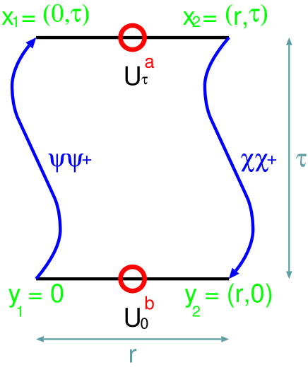
Figure 6.7: The four point function, $G_{ab}$.

In the derivation of the Schrödinger type bound state equation, Eq. (6.34), from Eq. (6.32) we have assumed that quarkonia can be completely classified by the quantum numbers of the constituent quarks. If this is not the case, the two-particle Green function, $G$, of Eq. (6.28) and Figure 6.5 has to be generalised to the $G_{ab}$ of Figure 6.7, where the indices, $a$ and $b$, run over all excitations that will contribute to the $J^{PC}$ of interest. To account for energy level shifts of $S$ wave vector mesons, $\Upsilon(nS)$, to order $c^{-2}$, clearly only $a,b=\Sigma_{g}^{+},\Sigma_{u}^{-},\Pi_{u}$ are relevant. All other channels decouple to this order in $c^{-1}$. The Hamiltonian, $H$, acts on $G_{ab}$,

$$-\frac{d}{dt}G_{ac}=\sum_{b}H_{ab}G_{bc},$$ (6.127)

and the resulting Schrödinger equation reads,

$$\sum_{b}H_{ab}\psi_{nJ^{PC}}^{b}({\mathbf{r}})=E_{nJ^{PC}}\psi_{nJ^{PC}}^{a}({\mathbf{r}}).$$ (6.128)

The normalisation is such that, $\sum_{a}\langle\psi_{a}|\psi_{a}\rangle=1$. Note that the state vector, $(\psi^{a}_{nJ^{PC}})$, now contains information about gluonic excitations too.

The ${\mathcal{O}}(1)$ Hamiltonian is diagonal in the space of hybrid excitations and, to this order, ${\mathbf{K}}$, ${\mathbf{S}}$ and $\Lambda^{\sigma_{v}}_{\eta}$ are separately conserved. However, to ${\mathcal{O}}(c^{-2})$, off-diagonal elements appear and the direction of $\psi$ will change with time. To compute the off-diagonal elements of $H$ we introduce $W_{ab}$, Wilson loops where the spatial transporter at $t=0$ is in representation $b$ of $D_{\infty h}$ and at $t=\tau$ in representation $a$. The orthogonality of states within different representations of $D_{\infty h}$ implies, $\langle W_{ab}\rangle=\delta_{ab}\langle W_{a}\rangle$. We now intend to relate the generalised four point function, $G_{ab}$, to the expectation value of $W_{ab}$, with appropriate colour field insertions on the temporal lines. Let us first consider the corrections from fluctuations around the static propagator, ${\mathbf{x}}_{2}(t)={\mathbf{r}}+{\mathbf{v}}(t-\tau/2)$. The expectation value of the perturbed Wilson loop, $W^{\mathbf{v}}_{ab}$, can be related to that of the static Wilson loop,

$$\langle W^{\mathbf{v}}_{ab}\rangle=\langle W_{ab}\rangle+{\mathbf{v}}g\int_{-\tau/2}^{\tau/2}\!dt\,t\,\langle{\mathbf{E}}({\mathbf{r}},t)W_{ab}\rangle:$$ (6.129)

the integral vanishes, unless the expectation value is negative under time reversal, $CP=T=-1$, in which case the correction matrix element itself disappears. We conclude that to the lowest non-trivial order, electrically mediated transitions between different hybrid potentials do not exist.

Next, we consider magnetic transitions. The relevant perturbation term, $\Delta H_{\mbox{\scriptsize ss}}({\mathbf{x}})$, is given in Eq. (6.78). In analogy to Eq. (6.77), we obtain,

$$H_{ab}=\frac{\langle a|\Delta H_{\mbox{\scriptsize ss}}|b\rangle}{(\langle a|a\rangle\langle b|b\rangle)^{1/2}}.$$ (6.130)

We have introduced the denominator, such that $|a\rangle$ and $|b\rangle$ do not need to be normalised. In the equal mass case the matrix element can be expressed in terms of Wilson loops in the following way, where we have exploited the fact that ${\mathbf{B}}$ is even under parity inversions and, ${\mathbf{S}}={\mathbf{S}}_{1}+{\mathbf{S}}_{2}$,

$$H_{ab}(r) = \frac{c_{F}(m)S_{i}}{m}V_{ab,i}(r),$$ (6.131)

$$V_{ab,i}(r) = g\,\lim_{\tau\rightarrow\infty}\langle\langle B_{i}({\mathbf{0}},\tau/2)\rangle\rangle_{ab},$$ (6.132)

where,

$$\langle\langle F\rangle\rangle_{ab}=\frac{\langle\mbox{Tr}(U_{ab}F)\rangle}{(\langle W_{a}\rangle\langle W_{b}\rangle)^{1/2}}.$$ (6.133)

$U_{ab}$ is a path ordered product of $SU(N)$ matrices, starting from and ending at the space-time position of $F$, with $\mbox{Tr}\,U_{ab}=W_{ab}$. Note that $V_{ab,i}=V_{ba,i}$ have dimension $m^{2}$.

If we are interested in corrections to $\Sigma_{g}^{+}$ states only, it is sufficient to consider the leading order diagonal elements,

$$H_{0,a}=2(\tilde{m}-\delta m)+\frac{p^{2}}{\tilde{m}^{2}}+V_{a}(r),$$ (6.134)

where $V_{a}$ denotes the respective hybrid potential. We can start from the unperturbed (diagonal) Hamiltonian, $H_{0}$, and determine the spectrum in all hybrid channels,

$$H_{0,a}\psi^{0,a}_{N}=E^{0,a}_{N}\psi^{0,a}_{N}.$$ (6.135)

Subsequently, the order $c^{-2}$ corrections to the $\Sigma_{g}^{+}$ levels can be determined in perturbation theory, the corrections to the diagonal part, $H_{0,{\Sigma_{g}^{+}}}$ in first (and, for spin-spin interactions as well as MD corrections, second) order, the corrections due to mixing with hybrids, $\Delta E_{N}^{mix}$, in second order,

$$\Delta E_{N}^{mix}=\sum_{M,a\neq\Sigma_{g}^{+}}\frac{\left|\langle\psi^{0,\Sigma_{g}^{+}}_{N}|H_{\Sigma_{g}^{+},a}|\psi^{0,a}_{M}\rangle\right|^{2}}{E_{M}^{0,a}-E_{N}^{0,\Sigma_{g}^{+}}}.$$ (6.136)

Note that radial excitations like $3S$ and $4S$ whose energy levels are close to those of hybrid states, will be more strongly affected by the mixing than $1S$ or $2S$ states, that are separated from the hybrids by substantial energy gaps. Also note that although the above equation very much resembles the general form of Eq. (6.77), in Eq. (6.136) static hybrid state creation operators are substituted by wave functions of quarkonia bound states, and hybrid potentials by ($r$-independent) quarkonia energy levels.

In QED similar mixing effects between $|e^{+}e^{-}\rangle$ states and $|e^{+}e^{-}\gamma\rangle$ states exist [416, 417, 418]. In QCD such effects are naïvely enhanced by factors, $\alpha_{s}v^{2}_{\Upsilon}/(\alpha_{fs}v^{2}_{e^{+}e^{-}})$, with respect to QED, however, the denominator of Eq. (6.136) guarantees an additional suppression; the lowest hybrid level is well separated from the ground state and the spectrum of hybrid potentials is discrete, rather than continuous. In addition to transitions between the ground state string and hybrid excitation, glueball creation can be considered. However, with masses of 3 – 4 GeV, the vector and axial-vector glueballs will only play a minor rôle while the scalar glueball will only enter the scenario at order $c^{-4}$, when quadrupole transitions have to be considered. In the case of QCD with sea quarks, additional flavour singlet meson channels open up, however, these particles are rather heavy too. Another possibility is the (OZI suppressed) radiation of three $\pi$s. The main change with respect to the quenched approximation is related to the spectra of static potentials at large $r$, where string breaking becomes possible. This will give rise to mixing effects with $B\overline{B}$ states.

It is interesting to observe that Eq. (6.128), which corresponds to the Lagrangian,

$${\mathcal{L}} = -\left(\psi_{\Sigma_{g}^{+}}^{\dagger}H_{\Sigma_{g}^{+}}\psi_{\Sigma_{g}^{+}}+\psi_{\Sigma_{u}^{-}}^{\dagger}H_{\Sigma_{u}^{-}}\psi_{\Sigma_{u}^{-}}+\cdots\right.$$ (6.137)

$$+ \left.\psi_{\Sigma_{g}^{+}}^{\dagger}H_{\Sigma_{g}^{+},\Sigma_{u}^{-}}\psi_{\Sigma_{u}^{-}}^{\dagger}+\psi_{\Sigma_{u}^{-}}^{\dagger}H_{\Sigma_{g}^{+},\Sigma_{u}^{-}}\psi_{\Sigma_{g}^{+}}+\cdots\right),$$

somewhat resembles the general form of the pNRQCD Lagrangian, Eq. (6.5.2). In our case, $\psi_{\Sigma_{g}^{+}}$ replaces the singlet wave function, $S$, while the octet finds its analogue in various hybrids. An important difference is that, unlike in Eq. (6.5.2), the leading order mixing elements contain magnetic fields while electric contributions proportional to, ${\mathbf{r}}\cdot{\mathbf{E}}$, have been found to vanish. Of course in higher orders of pNRQCD similar magnetic terms will appear too.

The potential approach not only allows all sorts of effects to be systematically incorporated but also enables the determination of many quantities that are not directly observable, for example the spectra of would-be hybrid states and the mixing matrix elements between these states and quark model states. This information is hidden in a direct lattice simulation. The results can readily be translated into languages commonly used in the context of the quark model and flux tube extensions thereof and put otherwise only heuristically defined concepts onto a firm basis. It also becomes obvious that the heavy quark interaction potential will only converge towards the static potential in the limit $v/c\rightarrow 0$, rather than $m\rightarrow\infty$ as one naïvely might have assumed, ignoring the kinetic term in the NRQCD Lagrangian. However, unlike in heavy-light systems, $v/c$ is not proportional to $m$ but $v/c\propto\alpha_{R}(r)$ [Eq. 6.1]: the desired limit $v/c\rightarrow 0$ will be approached logarithmically slowly as the spatial extent $r$ of the bound state wave function vanishes. This freezing of $v/c$ as a function of the quark mass $m$ at large $m$ is also illustrated by the estimates in the last row of Table 6.1.

6.6 Lattice determinations of the potentials

The potentials, Eqs. (6.56) – (6.3.4), are given in a form in which they can be easily evaluated on the lattice. Spin dependent potentials have been computed in $SU(2)$ gauge theory [402, 419, 420, 400, 401], $SU(3)$ gauge theory [421, 422, 423, 420, 424, 330, 29] and in exploratory studies of QCD with sea quarks [425, 426]. In Refs. [400, 29] the momentum dependent corrections in $SU(2)$ and $SU(3)$ gauge theories, respectively, have been considered too. The correction to the central potential, $V_{\prime}$, of Eq. (6.58) [32] as well as the transition potentials, $V_{ab,i}$, of Eq. (6.132), however, have not been calculated so far.

6.6.1 The method

The simplest discretisations of magnetic and electric field insertions, $g{\mathbf{B}}$ and $g{\mathbf{E}}$, are the clover leaf definitions of Eqs. (5.3) – (5.6). Alternative discretisations have been investigated in the first lattice study [402] of spin dependent potentials. Since the temporal lattice extent is always finite, the limit, $\tau\rightarrow\infty$, cannot be performed exactly. Moreover, the arguments of the integrals within Eqs. (6.56) – (6.3.4) can only be obtained on a discrete set of $t$ values. Spectral representations of the potentials, Eqs. (6.69) – (6.73), however, are extremely useful to guide and control interpolations and extrapolations as well as in improving the lattice operators used.

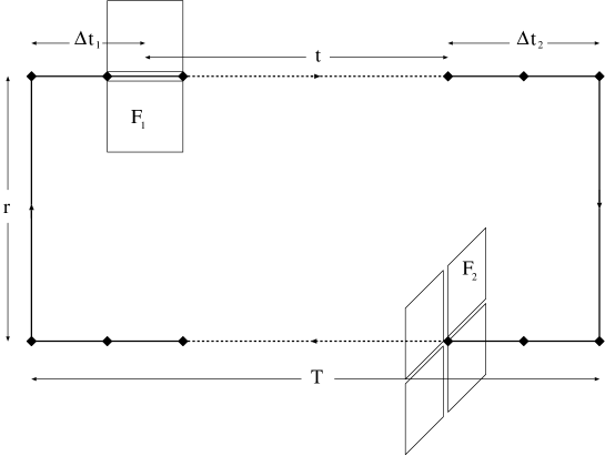
Figure 6.8: Lattice definition of the operator in the argument of the nominator of Eq. (6.68) for the example of $F_{1}$ being an electric and $F_{2}$ being a magnetic field.

Relative statistical errors explode with the temporal extent of a Wilson loop, $T\geq\tau$, while the distances between the field strength insertions and the spatial closures of the loop, $\Delta t_{1}$ and $\Delta t_{2}$, determine the degree of pollution from excited states. Therefore, adapting the size of the Wilson loop within the double bracket expectation value, Eq. (6.68), to the distance between the two field insertions, $t$, $T(t)=\Delta t_{1}+\Delta t_{2}+t$, turns out to be the optimal choice in terms of statistical errors as well as in terms of a fast convergence to the asymptotic limit of interest [401]. The resulting lattice operator is depicted in Figure 6.8. In addition to keeping $\Delta t_{i}$ large, the overlap with the ground state can be enhanced by smearing the spatial connections within the Wilson loop (cf. Section 4.7.1). In the first lattice studies [421] the integrals, Eqs. (6.56) – (6.3.4), were replaced by discrete lattice sums. By parameterising the arguments as continuous functions of $t$ [330, 29], prior to the integration, discretisation errors can be reduced and the effects of the region of large $t$ (where statistical errors dominate the signal) can still be incorporated. If the hybrid potentials are known, the exponents of such multi-exponential fits to Eqs. (6.69) – (6.73) can be determined independently [330, 419, 420].

6.6.2 Matching to the continuum

In all lattice studies, based on naïve discretisations of the continuum expressions, the potentials $V_{2}^{\prime},V_{3}$ and $V_{4}$ have been found to be much smaller than one would have expected from perturbative arguments or quarkonia phenomenology. In Ref. [402] this has been attributed to the anomalous dimension of the magnetic moment while in Ref. [421] this has been interpreted as a lattice artefact. As we shall see, both suggestions are true in parts. In particular the difference, $V_{2}^{\prime}-V_{1}^{\prime}$, has been found to be a factor of three to four times smaller [419, 423, 420] than the inter-quark force $V_{0}^{\prime}$, in violation of the Gromes relation, Eq. (6.48).

Nowadays, we know that such behaviour is caused by large renormalisations between lattice operators and their continuum counterparts [29]. In addition, the matching coefficients between NRQCD and QCD, discussed in Section 6.1, will affect quarkonium spectrum predictions. We can separately perform two matchings: lattice NRQCD to continuum NRQCD and continuum NRQCD to QCD. In Ref. [419] a procedure reminiscent of “tadpole improvement” [120] has been suggested to reduce the former renormalisation factor: the lattice operators are improved by dividing out factors, $U_{P}^{2}$, from the double bracket correlation functions. This prescription does not affect the continuum limit and still the leading order lattice artefacts are proportional to $a^{2}$. However, in perturbation theory all lattice specific one loop self-interactions of the field insertions are cancelled. This procedure can be refined by the Huntley-Michael (HM) construction [420], in which additional un-wanted higher order graphs cancel too. This becomes possible by taking the relative position of the field insertions with respect to the Wilson loop into account. This HM scheme has been employed in the simulations of Refs. [400, 401, 29], and as a result the Gromes and BBP relations Eqs. (6.48) – (6.50) are found to be respected within the achieved numerical accuracy of a few per cent.

Figure 6.9: The potential $\nabla^{2}V_{a}^{E}$, together with a fit curve, $\nabla^{2}V_{a}^{E}=-(2\sigma+b)/r$.

It has been suggested [423] to fix the lattice renormalisation factors non-perturbatively from the Gromes relation at distances, $r\gg a_{\sigma}$, where rotational symmetry is effectively restored on the lattice. From Eqs. (6.69) – (6.73) it is evident that the relativistic corrections to the static potential, rather than being spectral quantities themselves, are proportional to amplitudes, $D_{n}^{(i)}({\mathbf{r}})$, which will undergo renormalisation. Ratios of these amplitudes for different $n$, however, should approach the continuum ratios, up to order $a^{2}$ scaling violations. Let us define the renormalisation constants, $Z_{\mathbf{B}}({\mathbf{r}})$ and $Z_{\mathbf{E}}({\mathbf{r}})$,

$$\langle\Phi_{{\mathbf{r}},0}|{\mathbf{B}}({\mathbf{0}})|\Phi_{{\mathbf{r}},n}\rangle = Z_{\mathbf{B}}({\mathbf{r}})\langle\Phi_{{\mathbf{r}},0}|{\mathbf{B}}^{L}({\mathbf{0}})|\Phi_{{\mathbf{r}},n}\rangle$$ (6.138)

$$\langle\Phi_{{\mathbf{r}},0}|{\mathbf{E}}({\mathbf{0}})|\Phi_{{\mathbf{r}},n}\rangle = Z_{\mathbf{E}}({\mathbf{r}})\langle\Phi_{{\mathbf{r}},0}|{\mathbf{E}}^{L}({\mathbf{0}})|\Phi_{{\mathbf{r}},n}\rangle,$$ (6.139)

where $n$ should be chosen such that the corresponding amplitude does not vanish. From considerations analogous to Eq. (6.74) it is obvious that $V_{1}^{\prime}$ and $V_{2}^{\prime}$, measured on the lattice, have to be multiplied by factors $Z_{E}Z_{B}$, $V_{3},V_{4}$ and $\nabla^{2}V_{a}^{B}$ by factors $Z_{B}^{2}$ and all other potentials by $Z_{E}^{2}$ to make contact with the potentials in a continuum scheme.

Figure 6.10: The spin-orbit potential $V_{1}^{\prime}$, with a fit, $-V_{1}^{\prime}=\sigma+h/r^{2}$.

The definitions of $Z_{\mathbf{B}}$ and $Z_{\mathbf{E}}$ are ambiguous; any term that vanishes at least like $a^{2}$ can be added. Since the left hand sides of Eqs. (6.138) and (6.139) are approached by the right hand sides in the continuum limit, $Z_{\mathbf{B}}$ and $Z_{\mathbf{E}}$ are $r$ independent, up to order $a^{2}$ lattice artefacts, and can be defined from the value at $r=r_{0}$, for instance. Therefore, we only have to distinguish between four independent renormalisation factors, $Z_{B,\perp}$, $Z_{B,\|}$, $Z_{E,\perp}$ and $Z_{E,\|}$, where $\perp$ refers to a component orthogonal to the inter-quark axis and $\|$ parallel to the axis. By demanding the Gromes relation, Eq. (6.48), to hold for $r\approx r_{0}$, different linear combinations of products between $Z_{\mathbf{E}}$ and $Z_{\mathbf{B}}$ components can be determined. By varying the direction of ${\mathbf{r}}$, the three combinations, $Z_{B,\|}Z_{E,\perp}$, $Z_{B,\perp}Z_{E,\|}$ and $Z_{B,\perp}Z_{E,\perp}$, can be fixed. From the BBP relations, Eqs. (6.49) and (6.50), all $Z_{E}Z_{E}$ products can be over-determined. Therefore, a completely non-perturbative evaluation of the renormalisations required to restore the continuum Lorentz symmetry is viable. From the rotational symmetry of the relativistic correction potentials, observed in Ref. [29], one can conclude $Z_{B,\parallel}\approx Z_{B,\perp}$ as well as $Z_{E,\parallel}\approx Z_{E,\perp}$. In fact, up to the inherent order $a^{2}$ ambiguity, one would expect such (approximate) equalities if one considers that the renormalisation between lattice and continuum NRQCD is an ultra-violet effect and, therefore, should be primarily related to properties of the local field strength insertions themselves, rather than to their interaction with the ultra-soft background of bound state gluons. Moreover, using the same argument, on an isotropic lattice, $a_{\sigma}=a_{\tau}$, one would expect, $Z_{E}\approx Z_{B}$.

6.6.3 Results

We conclude this section by reviewing the lattice results obtained in the most concise and precise study so far [29]. The $SU(3)$ potentials have been determined by use of the quenched Wilson action on isotropic lattices at $\beta=6.0$ and $\beta=6.2$, that correspond to lattice spacings, $a^{-1}\approx 2.14$ GeV and $a^{-1}\approx 2.94$ GeV, respectively. In this reference, the HM renormalisation procedure [420] has been employed. Subsequently, the continuum Gromes and BBP relations were found to be satisfied within the statistical accuracy of the study.

Figure 6.11: The spin-orbit potential $V_{2}^{\prime}$, in comparison with the expectation, Eq. (6.84).

In Figure 6.9, we display the result for $\nabla^{2}V_{a}^{E}$, together with a fit of the form of Eq. (6.81). $\nabla^{2}V_{a}^{B}$ was found to be consistent with a constant. In the Figure, we have subtracted the fitted self-energy constants, $C_{a}^{E}a$, from the data points. The resulting $c_{D}C_{a}^{E}a\approx-1$ seemed to cancel $c_{F}^{2}C_{a}^{B}a\approx 1$ almost perfectly. At $\beta=6.0$ and $\beta=6.2$, values, $b=(1.13\pm 0.45)\sigma$ and $b=(1.83\pm 0.61)\sigma$, have been found, respectively. The sign of the difference, although not statistically significant, coincides with the expectation that the matching coefficient $c_{D}$ decreases with the lattice spacing [Figure 6.4]. Note that a value, $b\neq 0$, is incompatible with Eq. (6.4.3) that results from the assumption that the form factors, $\tilde{V}_{i}$, within the interaction kernel, Eq. (6.110), only depend on the momentum transfer, $q^{2}$.

The observation, $3c_{D}b+2\sigma>0$, means that besides the $\delta$ like Darwin term, another $1/r$ like mass- (and, therefore, flavour-) dependent correction to the central potential, with a coefficient of approximate size, $-2\,\sigma/(4m^{2})$, exists. However, this correction, together with an additional $-\sigma/(6m^{2})$ term from the MD potentials, yields an increase in the effective Coulomb coefficient of the Cornell potential of less than 2.5 % for bottomonium. In the case of charmonium the situation is less clear: the uncertainty in $c_{D}$ can result in an increase of the effective Coulomb coefficient of anything from 8 % to 18 %. The effective Coulomb coupling within the static potential will weaken at short distances as soon as one goes beyond the tree level inspired Cornell parametrisation. This is, however, not the case for the coefficient of the mass dependent corrections proportional to, $\nabla^{2}(V_{0}-V_{0,{\mbox{\scriptsize pert}}})\approx 2\sigma/r$ whose relative weight will, thus, increase at very short distances. Considering the discussion of the potential at very short distances in Section 4.8, such contributions could turn out to be more important than one would have assumed, guided by the Cornell parametrisation alone.

Figure 6.12: The spin-spin potential, $V_{3}$, in comparison with the expectation, Eq. (6.85).

In Figure 6.10, the long range spin-orbit potential $V_{1}^{\prime}$ is displayed, together with a fit of the form Eq. (6.83), where the string tension has been taken from a fit to the central potential. The values, $h=0.071\pm 0.013$ and $h=0.065\pm 0.009$, have been found at the two lattice spacings, respectively. Therefore, the dimensionless parameter $h$ turns out to be somewhat bigger than one fifth of the Coulomb coefficient, $e\approx 0.3$. Since $c_{F}$ increases with decreasing $a$, we expect $h$ to decrease slightly as a function of the lattice spacing. We can ask ourselves at what lattice spacing, $a^{\prime}\approx 1/\mu^{\prime}$, we would expect $h$ to assume its (unmixed) value, $h=0$. From Eq. (6.52), we can derive the relation, $c_{F}(\mu^{\prime})=[(e-h)/e]\,c_{F}(\mu)\approx 0.78\,c_{F}(\mu)$: a decrease of $c_{F}$ by more than 20 % is required which, as can be seen from Figure 6.2, will correspond to a scale (much) smaller than 1 GeV.

In Figures 6.11 and 6.12, we display $V_{2}^{\prime}$ and $V_{3}$, together with the model expectations of Eqs. (6.84) and (6.85). After having determined $e$ from the static potential and $h$ from $V_{1}^{\prime}$ there are no free parameters in the function displayed. Excellent agreement between the data and the predictions is found. $V_{2}^{\prime}$ does not contain any long distance contribution and therefore can be identified with the vector potential, $V_{V}$, within models that are based on an interaction kernel that only depends on the momentum transfer, i.e. $\eta=0$, within Eq. (6.114). The fact that $V_{3}\approx V_{2}^{\prime}/r-V_{2}^{\prime\prime}$ implies [Eq. (6.115)] $V_{P}(r)\approx cr^{2}$ and, therefore, $V_{P}\approx 0$.

Figure 6.13: The spin-spin potential, $V_{4}$, in lattice units at $\beta=6.2$, in comparison with the expectation, Eq. (6.86), and a one loop perturbative improvement.

In Figure 6.13, we display the potential $V_{4}$, determined at $\beta=6.2$ in lattice units. We decided not to plot the potential in physical units since the behaviour expected from Eq. (6.86) is a $\delta$ function. Hence, the result will be cut-off and discretisation dependent. For the clover leaf definition of the magnetic fields, employed in the study, the lattice $\delta$ function has been calculated (indicated as “tree level” in the plot). Indeed, the data are described well by this expectation. A one loop improved version brings the data even more in line with the expectation.

Figure 6.14: The potential, $V_{d}$, together with the curve $V_{d}(r)=-\sigma/9\,r$.

The errors in the lattice determination of the relativistic correction potentials are much bigger than those on the static potential of Figure 4.2. However, one should keep in mind that the effect of these terms on the spectrum is suppressed by factors of $v^{2}/c^{2}$ with respect to the static potential; even an error as big as 10 % on a 10 % correction term is completely tolerable for most phenomenological purposes as the induced uncertainty of a few MeV on the $\Upsilon$ spectrum will still be smaller than the effect of neglecting higher order relativistic or radiative corrections. In general, operators involving electric field insertions result in stronger statistical fluctuations than magnetic fields. Therefore, $V_{3}$ and $V_{4}$ are the most precisely determined potentials, followed by $V_{1}^{\prime}$ and $V_{2}^{\prime}$ while $\nabla^{2}V_{a}^{E}$ as well as the MD corrections are subject to big statistical uncertainties.

In the case of the MD potentials, this is particularly disappointing as the expectations, Eqs. (6.88) – (6.91), all contain a long range part and are all numerically small, in comparison with the other potentials. This means of course that these potentials are not of prime phenomenological interest. However, being dominated by non-perturbative effects, they are needed to discriminate between competing predictions arising from different assumptions on the QCD vacuum [60, 61]. As an example of a MD potential, $V_{d}(r)$ is depicted in Figure 6.14, together with the expectation, Eq. (6.90). The fitted self-energies $C_{d}$ have been subtracted from the data sets. Note that the BBP relation, Eq. (6.49), has been confirmed to hold for the self-energies, $2C_{b}+4C_{d}+V_{\mbox{\scriptsize self}}=0$. Clearly, further improved numerical simulations are required to arrive at definite conclusions about the functional form of the MD potentials.

7 Application to the quarkonium spectrum

After having determined the potentials, quarkonia spectra and wave functions can readily be predicted, within the limitations of the non-relativistic and adiabatic approximations. Vice versa, quarkonium spectra can in principle be used as an input to fix parameters that have not yet been determined accurately, in particular the matching coefficients appearing within the effective action. The same values could then be taken in lattice NRQCD studies or HQET calculations of heavy-light bound states and their decay matrix elements. In particular, the $S$ and $P$ state fine splittings react in a very sensitive way towards variations of these coefficients. Unfortunately, the $\eta_{b}$ whose splitting with respect to $\Upsilon$ states would yield the cleanest information has not been discovered yet. Moreover, the fine structure as well as decay rates, that are proportional to the wave function (or in the case of $P$ states, its derivative) at the origin, probe the heavy quark interaction at very small distances. Here we will restrict our discussion to spectrum determinations and estimations of the systematic errors inherent in order $v^{4}$ (or $c^{-2}$) continuum and lattice NRQCD as well as uncertainties from neglecting sea quarks.

7.1 Solving the Schrödinger equation

Once the interaction potentials are determined, the Schrödinger equation, Eq. (2.8), can be solved numerically on any personal computer, either on a discrete lattice [30] or in the continuum [12, 16, 17]. In the latter case, one would start by integrating the radial equation, Eq. (A.2) or Eq. (A.10), for the Hamiltonian $H_{0}$ of Eqs. (6.4.2) and (6.106),

$$H_{0}|nll_{3}\rangle=E_{nl}^{0}|nll_{3}\rangle.$$ (7.1)

Subsequently, the $1/m^{2}$ corrections, Eqs. (6.98) – (6.100), can be treated as perturbations,

$$E_{nJls}=E_{nl}^{0}+\frac{1}{\tilde{m}^{2}}\sum_{i}\langle{nll_{3}}|\delta H_{i}(r,J,l,s,{\mathbf{p}})|{nll_{3}}\rangle.$$ (7.2)

By use of the identities [16, 30],

$$\langle nll_{3}|f(r)p^{2}|nll_{3}\rangle = \tilde{m}\left\langle nll_{3}\left|f(r)\left[E_{nl}^{0}-\tilde{V}(r)\right]\right|nll_{3}\right\rangle,$$ (7.3)

$$4\pi\langle nll_{3}|\delta^{3}(r)|nll_{3}\rangle = \left|\psi_{nll_{3}}(0)\right|^{2}$$

$$= \frac{\tilde{m}\sigma}{\pi}\left(1+\frac{\tilde{e}}{\sigma}\langle nll_{3}|r^{-2}|nll_{3}\rangle\right),$$

all perturbations can readily be computed from expectation values, $\langle r^{\alpha}\rangle$, $\alpha=-4,\ldots,1$. Note that $\tilde{m}$, $\tilde{V}(r)$ and $\tilde{e}$ are defined in Eqs. (6.105) – (6.109).

Figure 7.1: The bottomonium spectrum from the lattice potentials [29].

The Hamiltonian of Eqs. (6.4.2) – (6.100) originates from the parametrisations, Eqs. (6.80) – (6.91), of $V_{0}(r)$ – $V_{e}(r)$ that are in qualitative agreement with the lattice data. These lattice inspired parametrisations for intermediate and large distances can of course be combined with perturbative short range expectations [367, 258, 398], for example along the lines of Ref. [20], for the purpose of a phenomenologically more accurate description of bottomonia states. This is certainly worthwhile doing as soon as lattice results on the transition matrix elements discussed in Section 6.5.4 become available and some of the NRQCD matching coefficients, in particular $c_{F}$, have been determined in a non-perturbative way. Anticipating such future results we can, however, use the available lattice data to estimate systematic uncertainties that are due to radiative and relativistic corrections as well as neglecting sea quarks.

Before discussing such effects, we reproduce the bottomonium spectrum obtained in Ref. [29] from the lattice potentials in Figure 7.1. The displayed spectrum has been obtained from the parameter values,

$$e = 0.32,$$ (7.5)

$$h = 0.065,$$ (7.6)

$$b = 1.81\sigma=1.81(1.65-e)\,r_{0}^{-1},$$ (7.7)

$$C_{0} = 0,$$ (7.8)

$$\tilde{m}_{b} = 4.676\,\mbox{GeV},$$ (7.9)

$$r_{0}^{-1} = 406\,\mbox{MeV},$$ (7.10)

with one loop matching coefficients, $c_{F}$, $d_{v}$ and $c_{D}$. While $e$, $h$ and $b$ have been computed entirely on the lattice, the quark mass, $\tilde{m}_{b}$, and the scale, $r_{0}$, have been determined from a fit to the experimental spectrum.

The Figure illustrates the precision to which experiment can at present be reproduced, without recourse to phenomenological input other than that required to fix the quark mass and the scale. It is not a priori clear whether the average deviations of almost 20 MeV are dominantly caused by relativistic and radiative corrections or due to ultra-soft gluons that have not yet been incorporated into the potential approach. Uncertainties resulting from the statistical errors on the potentials as well as differences between data sets obtained at $\beta=6.0$ and $\beta=6.2$ cannot be resolved on the scale of the plot. In addition to results based on the fit parameters, extracted from the quenched simulations ($e=0.32$), results for a stronger Coulomb coupling, $e=0.40$, are displayed. We intend to model the changes that one might expect when including sea quarks by this latter choice of $e$. It is amusing to notice that, when ignoring the mass dependence of the matching coefficients, $c_{i}=1$, all ratios of splittings come out to be consistent [30] with those determined in direct lattice NRQCD simulations, indicating that higher order relativistic corrections as well as effects due to ultra-soft gluons do not play a prominent rôle, at least for the lowest few levels; all differences between published lattice NRQCD results and the spectrum of Figure 7.1 are entirely due to different prescriptions for assigning a physical scale to the lattice results and a different choice of the matching coefficients, $c_{i}$. In the potential case, overall agreement with experiment has been optimised while in lattice NRQCD usually the most precisely determined $2^{3}S_{1}-1^{3}S_{1}$ or $1\overline{{}^{3}P}-1^{3}S_{1}$ splittings are taken as the only input.

7.2 Systematic uncertainties

Having a Hamiltonian representation of the bound state problem at hand it is straight forward to investigate how the spectrum changes when the input parameters are varied. For instance, fine structure splittings are to first approximation proportional to the matching coefficient, $c_{F}^{2}$. Such effects are discussed in detail in Ref. [30]. Here, we briefly summarise the main results and discuss the uncertainties common to the potential and the lattice NRQCD approaches. In addition, the effect of neglecting sea quarks is investigated and finite volume effects for lattice studies of $\Upsilon$ properties are estimated.

Unfortunately, no precision results on the corrections to the static potential in QCD with sea quarks exist. However, the static potential has been determined accurately [246, 255, 167, 248, 247] for $n_{f}=2$ (cf. Section 4.7.4), and an increase of the effective Coulomb coefficient $e$ by 16 % to 22 % has been detected [167, 248] for quark masses, $m_{u}=m_{d}>m_{s}/3$ (cf. Figure (4.5).

Figure 7.2: $R=\Delta m_{2S1S}/\Delta m_{1P1S}$ as a function of $m_{\Upsilon}^{-1}$ for various values of the Coulomb coupling, $e$. The upper curves correspond to the lowest order Hamiltonian, the lower ones incorporate relativistic corrections.

The ratio,

$$R=\frac{m_{2^{3}S_{1}}-m_{1^{3}S_{1}}}{m_{1\overline{{}^{3}P}}-m_{1^{3}S_{1}}},$$ (7.11)

reacts in a very sensitive way towards quenching. The potentials yield $R\approx 1.38$ which (while in perfect agreement with quenched lattice NRQCD [386]) disagrees with experiment, $R\approx 1.28$. The dependence of $R$ on $e$, keeping the parameters $r_{0}^{-1}$ and $\tilde{m}$ fixed, is displayed in Figure 7.2. Values, $e\approx 0.4$, appear necessary for the real world with three active sea quark flavours to reproduce this ratio. Keeping in mind that two sea quarks resulted in the effective Coulomb strength to increase by about 20 %, such an increase by 30 % indeed appears to be very reasonable. Our suggested sizes of quenching effects will be based on this estimate. From the Figure it is also obvious that while order $v^{4}$ ($c^{-2}$) effects on this ratio are small around the bottom mass, relativistic corrections explode in an uncontrolled way towards the charm: while $\langle v^{2}\rangle_{\Upsilon}\approx 0.1$ for bottomonia, $\langle v^{2}\rangle_{J/\psi}\approx 0.4$ is not exactly a small expansion parameter anymore.

Table 7.1: Relativistic and radiative corrections to $\Upsilon$ splittings.

splitting	${\mathcal{O}}(v^{4})$	${\mathcal{O}}(v^{6})$	radiative
$2\overline{S}-1\overline{S}$	13 MeV	2 MeV	5 MeV
$2^{3}S_{1}-1^{3}S_{1}$	17 MeV	2 MeV	6 MeV
$1\overline{{}^{3}P}-1\overline{S}$	24 MeV	1.5 MeV	2 MeV
$1\overline{{}^{3}P}-1^{3}S_{1}$	12 MeV	1.5 MeV	5 MeV

Table 7.2: Relativistic and radiative corrections to $J/\psi$ splittings.

splitting	${\mathcal{O}}(v^{4})$	${\mathcal{O}}(v^{6})$	radiative
$2\overline{S}-1\overline{S}$	65 MeV	25 MeV	15 MeV
$1\overline{{}^{3}P}-1\overline{S}$	35 MeV	15 MeV	15 MeV

Table 7.3: Relativistic and radiative corrections to fine structure splittings.

family	${\mathcal{O}}(v^{6})$	radiative	quenching
$\Upsilon$	10 %	25 %	35 %
$J/\psi$	40 %	70 %	30 %

Relativistic ${\mathcal{O}}(v^{4})$ correction terms affect spin averaged $2\overline{S}-1\overline{S}$ splittings by about 2.5 % and 11 % for bottomonium and charmonium, respectively; the corresponding numbers for the $1\overline{{}^{3}P}-1\overline{S}$ splittings are 4 % and 8 %. No experimental values for $\overline{S}$ $\Upsilon$ states are available since pseudo-scalar $\eta_{b}$ mesons are not yet discovered. The $\Upsilon$ $2^{3}S_{1}-1^{3}S_{1}$ and $1\overline{{}^{3}P}-1^{3}S_{1}$ splittings that are therefore at present of greater interest become reduced by another 1 % and 2.5 % due to spin-spin interactions when switching on relativistic corrections. In Table 7.1, we display estimates [30] of the effect of even higher order relativistic correction terms on various $\Upsilon$ splittings as well as the size of error induced by ignoring the mass dependence of the matching coefficients between QCD and NRQCD when simulating the theory at lattice spacings, $1.5~{}$GeV $\leq a^{-1}\leq 3$ GeV. In Table 7.2, the corresponding results for $J/\psi$ states are displayed. To set the scale: $\Delta m_{2S1S}\approx 580$ MeV, $\Delta m_{1P1S}\approx 430$ MeV. Note that the order $v^{4}$ corrections have been calculated while order $v^{6}$ and radiative corrections are estimates only. Within order $v^{4}$ NRQCD, radiative corrections to the matching coefficients, that are of size $\alpha_{s}\log(m/\mu)/m^{2}$, dominate over relativistic correction terms that are accompanied by factors $1/m^{3}$, at least for bottomonia.

In Table 7.3 we summarise the estimates of the uncertainties of the fine structure splittings. Since we only have results from the lowest order at which the splittings can occur, the relative sizes of the relativistic corrections can only roughly be estimated to be of order $v^{2}$. We did not try to assign quenching errors to individual spin averaged splittings. Only mass ratios, and not the overall scale, can be determined from the QCD Lagrangian. Therefore, assigning a quenching error to an individual mass is highly subjective since the result will depend on the experimental input quantity used to fix the lattice spacing. One finds different scale determinations to scatter by up to 20 % within the quenched approximation which should be interpreted as the overall systematic uncertainty. In contradiction to this philosophy, estimates on quenching errors are given for the fine structure splittings. These are explicitly proportional to the Coulomb coupling. The quenching error estimates have to be interpreted as typical changes of the size of fine structure splittings with respect to spin averaged splittings. Including sea quarks will result in an increase of such ratios. The effect of radiative corrections goes in the same direction, this is obvious from the continuum two loop inspired estimate of Figure 6.2. Besides quenching, the latter uncertainty again seems to be the dominant source of error.

Indeed, using tree level matching coefficients, one underestimates $P$ wave fine structure splittings for $e=0.40$ by almost a factor two [30], compared to experiment. However, for the ratio,

$$R_{FS}=\frac{m_{\chi_{b2}}-m_{\chi_{b1}}}{m_{\chi_{b1}}-m_{\chi_{b0}}},$$ (7.12)

from which the dominant radiative correction cancels, one obtains $R_{FS}\approx 0.56$ which has to be compared to the experimental value, $R_{FS}\approx 0.66$. By incorporating running coupling effects into the parametrisation of $V_{3}$ and calculating order $v^{6}$ effects, it should be possible to further improve the agreement.

Figure 7.3: Difference between $\Upsilon$ levels and their infinite volume values as a function of the lattice extent, $La$.

The potential approach not only offers an intuitive and transparent representation of quarkonia bound state properties in a continuum context but it can also guide lattice simulations. By numerically solving the Schrödinger equation on a three-dimensional torus for instance finite size effects can be estimated. This has been done in Ref. [30], and the main result is displayed in Figure 7.3. While the approach to the infinite volume limit for $n=1$ states is monotonous, this is not so for radial excitations. Some states, in particular the $3S$, show a non-trivial behaviour that results in infinite volume extrapolations from data obtained at lattices with $a_{\sigma}L_{\sigma}<2$ fm to become uncontrolled. The relevant symmetry group on a torus (as well as on a discrete lattice) is $O_{h}$, rather than $O(3)$. The five-dimensional continuum $O(3)$ $D$ wave representation splits up into the two-dimensional $O_{h}$ representation, $E$, and the three-dimensional representation, $T_{2}$. It is amusing to see that rotational symmetry is not only broken for finite lattice spacing but also at any finite volume, with $1T_{2}$ approaching the continuum $1D$ state from above and $1E$ approaching it from below. If one aims at finite size effects below 3 MeV, a lattice extent $L_{\sigma}a\approx 1.5$ fm seems to suffice for $1S$ and $1P$ states while for $2S$, $2P$ and $1D$ states, $L_{\sigma}a\approx 2$ fm is required and for $3S$ or $3P$ even 2.5 fm become necessary. On a 1.5 fm lattice for instance one would underestimate the $3S$ level by more than 50 MeV.

8 Conclusions

QCD contains a rich spectrum of purely gluonic excitations. Glueballs and torelons that are colour singlet states can be realised, as well as glueballinos that transform according to the adjoint representation of the gauge group. Chromo electro-magnetic flux states between static colour sources in the fundamental or in higher representations of the gauge group can be constructed that have non-local gauge transformation properties. Besides mesonic potentials and hybrid excitations thereof, baryonic three-body potentials and even more complicated situations can be investigated.

All these excitations can be accessed in lattice simulations with much more ease than properties of states containing fermionic constituents. While the lattice reveals many interesting and non-trivial aspects of QCD in some cases it is hard to detect effects that very obviously do exist like the breaking of the hadronic string. Lattice results are extremely useful to test and improve models of low energy QCD. Moreover, phenomena like the Casimir scaling found between potentials between charges in different representations of the gauge group or the $\Delta$ law of baryonic potentials, provide some insight into hidden aspects of the dynamics of the theory. Such results give reason for optimism that once out of the chaos there might arise understanding. On the other hand QCD exhibits a complex vacuum structure, and even in the allegedly perturbative short distance domain non-perturbative effects seem to play a rôle in some cases.

QCD predicts the quark model as a classification scheme of hadronic states to be incomplete. Nonetheless, it seems to do quite well; in particular those gluonic excitations that would make a difference, come out to be quite heavy. The quark model can of course be improved by incorporating the known gluonic excitations. In doing so, one would expect the lightest quark-gluon spin exotica to be vectors, $J^{PC}=1^{-+}$. This result can be systematically derived for heavy quark bound states. However, direct lattice simulations show that it also applies to the light meson sector.

We have demonstrated that in a non-relativistic situation, it is possible to factorise gluonic effects from the slower dynamics of the quarks. This adiabatic approximation is violated when ultra-soft gluons are radiated, i.e. when the nature of the bound state changes during the interaction time. However, such effects can be incorporated into the potential formulation by enlarging the basis of states onto which the Hamiltonian acts. Moreover, the validity of the adiabatic approximation is tied to that of the non-relativistic approximation in so far as the transition matrix elements are suppressed by powers of the velocity, $v$.

Within the adiabatic framework, valence gluons that accompany the quarks in the form of hybrid excitations of the flux tube and sea gluons, whose average effect is parameterised in terms of interaction potentials, can be distinguished from each other. To lowest order of the relativistic expansion pure quark model quarkonia and quark-gluon hybrids exist, which then undergo mixing with each other as higher orders of the relativistic expansion are incorporated. Hybrid mesons become a well defined concept in the potential approach and translation into the variables used for instance in flux tube models is straight forward.

It has been shown that potential models can be systematically derived from QCD. An understanding of effective field theory methods turned out to be essential for this step. The resulting Hamiltonian representation of the bound state problem in terms of functions of canonical variables offers a very intuitive and transparent representation of quarkonium physics. It highlights parallels as well as differences to well understood atomic physics.

In view of phenomenological applications, a non-perturbative determination of the matching coefficients between QCD and lattice NRQCD is urgent. As an alternative to lattice NRQCD and the lattice potential approach, quarkonia properties can also be calculated from relativistic quarks by introducing an anisotropy, $a_{\tau}\ll a_{\sigma}$. However, the potential approach is unique in its capability to access high radial excitations and to determine wave functions. From a non-perturbative determination of the matching coefficients, simulations of heavy-light systems would benefit too. Another challenge is to generalise the results presented to heavy-light systems, i.e. to achieve a similar factorisation into sea (gluon and quark) effects and valence (quark and gluon) effects, within an expansion in terms of the inverse heavy quark mass, $m^{-1}$.

Appendix A The radial Schrödinger equation

For a rotationally symmetric potential, the standard substitution,

$$\psi_{nll_{3}}({\mathbf{x}})=\frac{u_{nl}(r)}{r}Y_{ll_{3}}(\theta,\phi),$$ (A.1)

into the Schrödinger equation, Eq. (2.8),

$$\left[\frac{{\mathbf{p}}^{2}}{2\mu_{R}}+V(r)\right]\psi_{nll_{3}}({\mathbf{x}})=E_{nl}\psi_{nll_{3}}({\mathbf{x}}),$$

results in the radial equation,

$$u^{\prime\prime}_{nl}(r)+2\mu_{R}\left[E_{nl}-V(r)-\frac{l(l+1)}{2\mu_{R}r^{2}}\right]u_{nl}(r)=0,$$ (A.2)

with $u(0)=0$, $u^{\prime}(0)=\psi({\mathbf{0}})$. In order to understand the dependence of the spectrum on the underlying potential, we discuss power law parametrisations,

$$V(r)=\lambda\,r^{\nu},\quad\nu=-1,1,2,\ldots.$$ (A.3)

The virial theorem implies,

$$\langle T\rangle=E-\langle V\rangle=\frac{\nu}{2+\nu}E,$$ (A.4)

where $T=p^{2}/(2\mu_{R})$ denotes the kinetic energy and $\langle T\rangle=\langle\psi_{nll_{3}}|T|\psi_{nll_{3}}\rangle$. For simplicity we have omitted the quantum numbers from Eq. (A.4). The average relative velocity of the heavy quarks within the bound state can easily be determined from Eq. (A.4),

$$\langle v^{2}\rangle=\frac{1}{\mu_{R}^{2}}\langle p^{2}\rangle=\frac{2}{\mu_{R}}\frac{\nu}{2+\nu}E,$$ (A.5)

whereas

$$\langle r^{\nu}\rangle=\frac{1}{\lambda}\langle V\rangle=\frac{1}{\lambda}\frac{2}{2+\nu}E.$$ (A.6)

Eq. (A.2) can be reformulated in terms of dimensionless variables by a simple scale transformation,

$$\rho = \left(2\mu_{R}|\lambda|\right)^{\frac{1}{2+\nu}}r,$$ (A.7)

$$\epsilon = 2\mu_{R}\left(2\mu_{R}|\lambda|\right)^{-\frac{2}{2+\nu}}E,$$ (A.8)

$$w(\rho) = u(r).$$ (A.9)

As a result, Eq. (A.2) reads,

$$w_{nl}^{\prime\prime}+\left[\epsilon_{nl}-\mbox{sign}(\lambda)\rho^{\nu}-\frac{l(l+1)}{\rho^{2}}\right]w_{nl}=0.$$ (A.10)

The primes now represent derivatives with respect to the argument $\rho$. The dependence of an energy splitting $\Delta E$ and a length scale $l$ on the coupling strength $\lambda$ and reduced mass $\mu_{R}$ is evident from Eqs. (A.8) and (A.7), respectively,

$$\Delta E\propto|\lambda|^{\frac{2}{2+\nu}}\mu_{R}^{-\frac{\nu}{2+\nu}},\quad l\propto\left(|\lambda|\mu_{R}\right)^{-\frac{1}{2+\nu}}.$$ (A.11)

For negative powers $\nu$, level spacings decrease with increasing quark mass, while for positive exponents, the opposite is the case.

A logarithmic potential, $V(r)=C\,\ln(r/r_{0})$, constitutes the limiting case between positive and negative $\nu$. Indeed, for such a parametrisation one obtains a velocity $\langle v^{2}\rangle=C/\mu_{R}$ as well as quark mass independent splittings, $\Delta E$ [224] while $l\propto r_{0}C^{1/2}/\mu_{R}^{1/2}$. For a Coulomb potential ($\nu=-1$) we obtain, $\Delta E\propto\lambda^{2}\mu_{R}$ and $l\propto 1/(\lambda\mu_{R})$ while a linear potential ($\nu=1$) yields $\Delta E\propto\lambda^{2/3}/\mu_{R}^{1/3}$ and $l\propto 1/(\mu_{R}\lambda)^{1/3}$. For a detailed discussion of the connection between spectrum and potential, we refer the reader to an excellent review article by Quigg and Rosner [16].

Appendix B Euclidean Field Theory

We summarise the conventions and notations used in this article. We start by translating some Euclidean space-time objects into Minkowski space-time (superscript $M$) with metric $\eta=\mbox{diag}(1,-1,-1,-1)$ for reference:

$$x_{i} = x^{i,M}=-x_{i}^{M},\quad x_{4}=ix^{0,M}=ix_{0}^{M},$$ (B.1)

$$\partial_{i} = \partial_{i}^{M}=\partial^{i,M},\quad\partial_{4}=-i\partial_{0}^{M}=-i\partial^{0,M},$$ (B.2)

$$\gamma_{i} = i\gamma^{i,M}=-i\gamma_{i}^{M},\quad\gamma_{4}=\gamma^{0,M}=\gamma_{0}^{M},$$ (B.3)

$$A_{i} = -A^{i,M}=A_{i}^{M},\quad A_{4}=-iA^{0,M}=-iA_{0}^{M},$$ (B.4)

$$F_{i4} = iF^{i0,M}=-iF_{i0}^{M},\quad F_{ij}=F^{ij,M}=F_{ij}^{M},$$ (B.5)

$${\mathbf{B}} = {\mathbf{B}}^{M},\quad{\mathbf{E}}=-i{\mathbf{E}}^{M}.$$ (B.6)

The above conventions conform to the anti-commutation relations $\{\gamma_{\mu},\gamma_{\nu}\}=2\delta_{\mu\nu}$ for the Dirac $\gamma$-matrices. $A_{\mu}$ denotes the electro-magnetic four-potential, $F_{\mu\nu}$ the Maxwell field strength tensor and ${\mathbf{E}}$ and ${\mathbf{B}}$ its components, the electric and magnetic fields. While in Minkowski notation Lorentz indices assume values $\mu=0,1,2,3$, in Euclidean notation, they run from 1 to 4.

We denote the generators of the $SU(N)$ group by $T^{a}$, with $a=1,\ldots,N_{A}$, $N_{A}=N^{2}-1$. They fulfil the commutation relations,

$$[T^{a},T^{b}]=if^{abc}T^{c},$$ (B.7)

with $f^{abc}$ being real, totally antisymmetric structure constants. In $SU(2)$ the generators can be represented in terms of Pauli matrices, $T^{i}=\sigma^{i}/2$, in $SU(3)$ by Gell-Mann matrices, $T^{a}=\lambda^{a}/2$. The vector potential lives in the Lie algebra,

$$A_{\mu}(x)=\sum_{a}A_{\mu}^{a}(x)T^{a},$$ (B.8)

while local gauge transformations generate the Lie group,

$$\Omega(x)=\exp[i\omega^{a}(x)T^{a}]\in SU(N).$$ (B.9)

Under a gauge transformation, $\Omega$, the field $A_{\mu}$ transforms in the adjoint representation,

$$A_{\mu}\rightarrow A_{\mu}^{\Omega}=\Omega[A_{\mu}-i\partial_{\mu}]\Omega^{\dagger}.$$ (B.10)

Fields that are in the fundamental representation of $SU(N)$, e.g. Dirac spinors, $q(x)$, transform like,

$$q(x)\rightarrow\Omega(x)q(x),\quad\bar{q}(x)\rightarrow\bar{q}(x)\Omega^{\dagger}(x).$$ (B.11)

The Dirac fermionic Lagrangian in Euclidian space reads,

$${\mathcal{L}}_{f}=\bar{q}(\gamma_{\mu}D_{\mu}+m)q,$$ (B.12)

with the covariant derivative,

$$D_{\mu}=\partial_{\mu}+iA_{\mu},$$ (B.13)

while the Euclidean Yang-Mills Lagrangian,

$${\mathcal{L}}_{YM}=\frac{1}{2g^{2}}\mbox{tr}\,(F_{\mu\nu}F_{\mu\nu})=\frac{1}{2g^{2}}\mbox{tr}\,(F_{\mu\nu}^{M}F^{\mu\nu,M})=-{\mathcal{L}_{YM}^{M}},$$ (B.14)

can be constructed from the field strength tensor,

$$F_{\mu\nu}=-i[D_{\mu},D_{\nu}]=\partial_{\mu}A_{\nu}-\partial_{\nu}A_{\mu}+i[A_{\mu},A_{\nu}].$$ (B.15)

The relative minus sign within Eq. (B.14) with respect to the Minkowski version implies that solutions of the classical equations of motion minimise the action, which is bounded from below. Therefore, quantum fluctuations are suppressed with respect to classical solutions by factors, $e^{-\delta S}$, within the path integral measure.

The phase and normalisation of the field strength tensor above is chosen such that,

$$gB_{i}=\frac{1}{2}\epsilon_{ijk}F_{jk},\quad gE_{i}=F_{i4},$$ (B.16)

correspond to the chromo-magnetic and electric fields, respectively. $g=\sqrt{4\pi\alpha_{s}}$ denotes the strong coupling “constant”. Note that our definition of the electric field, ${\mathbf{E}}=-i{\mathbf{E}}^{M}$, differs by a phase $i$ from some text book conventions, resulting in, $E^{a}_{i}E^{a}_{i}\geq 0$. The gauge action expressed in terms of the colour fields reads,

$$S_{YM}=\frac{1}{2}\int\!d^{4}x\,(E_{i}^{a}E_{i}^{a}+B_{i}^{a}B_{i}^{a}).$$ (B.17)

Appendix C The perturbative $\beta$-function

The one, two and three loop coefficients of the $\beta$-function, Eq. (3.22),

$$\beta(\alpha_{s})=\frac{d\alpha_{s}}{d\ln\mu^{2}}=-\beta_{0}\alpha_{s}^{2}-\beta_{1}\alpha_{s}^{3}-\beta_{2}\alpha_{s}^{4}-\ldots,$$

have been calculated in Refs. [427, 428], [429, 430, 431] and [432, 433], respectively, in the modified minimal subtraction $\overline{MS}$ scheme [434, 435, 436] of dimensional regularisation [437]. The $n_{f}$ flavour results for an $SU(N)$ gauge group read,

$$\beta_{0} = \left(\frac{11}{3}N-\frac{2}{3}n_{f}\right)\frac{1}{4\pi},$$ (C.1)

$$\beta_{1} = \left[\frac{34}{3}N^{2}-\left(\frac{13}{3}N-\frac{1}{N}\right)n_{f}\right]\frac{1}{16\pi^{2}},$$ (C.2)

$$\beta_{2}^{\overline{MS}} = \left[\frac{2857}{54}N^{3}-\left(\frac{1709}{54}N^{2}-\frac{187}{36}-\frac{1}{4N^{2}}\right)n_{f}\right.$$

$$+ \left.\left(\frac{56}{27}N-\frac{11}{18N}\right)n_{f}^{2}\right]\frac{1}{64\pi^{3}},$$

while the four-loop coefficient $\beta_{3}^{\overline{MS}}$ has been calculated in Ref. [438]. The latter reference also contains the coefficients for all compact semi-simple Lie gauge groups. The conversion between $\overline{MS}$ scheme couplings and the bare lattice coupling for Wilson gluonic and fermionic action is know to two loops [391, 392, 393, 394, 439, 440]. The numerical pure gauge result for the $\beta$ function coefficient $\beta_{2}^{L}$ reads [441, 442],

$$\beta_{2}^{L}\approx\left(-366.2N^{3}+1433.8N-\frac{2143}{N}\right)\frac{1}{64\pi^{3}},$$ (C.4)

while for $SU(3)$ with $n_{f}$ flavours of Wilson fermions one obtains [440],

$$\beta_{2}^{L}\approx\left(-6299.9-1067n_{f}+59.89n_{f}^{2}\right)\frac{1}{64\pi^{3}}.$$ (C.5)

Translating between one scheme and another is straight forward: from

$$\alpha^{\prime}(\mu)=\alpha(\mu)+c_{1}\alpha^{2}(\mu)+c_{2}\alpha^{3}(\mu)+c_{3}\alpha^{4}(\mu)+\cdots,$$ (C.6)

one obtains,

$$\beta_{0}^{\prime} = \beta_{0},\quad\beta_{1}^{\prime}=\beta_{1},$$ (C.7)

$$\beta_{2}^{\prime} = \beta_{2}-c_{1}\beta_{1}+(c_{2}-c_{1}^{2})\beta_{0},$$ (C.8)

$$\beta_{3}^{\prime} = \beta_{3}-2c_{1}\beta_{2}+c_{1}^{2}\beta_{1}+2(c_{3}-3c_{1}c_{2}+2c_{1}^{3})\beta_{0},$$ (C.9)

$$\Lambda^{\prime} = \Lambda\,e^{c_{1}/(2\beta_{0})}.$$ (C.10)

Appendix D The centre symmetry

On a torus, a global $Z_{N}$ symmetry is associated with each compactified space-time direction, $\mu$, besides the invariance of the action and path integral measure under local gauge transformations. $Z_{N}$ denotes the set of the $N$ $N$th roots of unity and $z\in Z_{N}\subset SU(N)$. This means,

$$[z,U_{x,\mu}]=0.$$ (D.1)

Multiplying all links crossing a hypersurface perpendicular to the $\mu$ direction by a factor $z$,

$$U_{x,\nu}\rightarrow U_{x,\nu}^{z}=\left\{\begin{array}[]{l}z\,U_{x,\nu}\quad\forall\quad x_{\mu}=0,\quad\nu=\mu\\ U_{x,\nu}\quad\mbox{otherwise}\end{array}\right.,$$ (D.2)

leaves traces of closed loops of link variables with trivial winding number around the boundary in $\mu$-direction invariant: since every such loop crosses every hypersurface an even number of times, all factors $z$ that are collected when crossing in the positive direction are cancelled by the $z^{*}$ factors collected from negative crossings. In particular, this argument applies to all pure gauge $SU(N)$ actions which are linear combinations of traces of such loops. The fermionic part of the action, containing a covariant derivative, however, explicitly violates this $Z_{N}$ invariance.

D.1 The Polyakov line and deconfinement

The position of the hypersurface of Eq. (D.2) can be moved by means of ordinary gauge transformations. Therefore, in infinite volume, it can be sent to infinity and the centre symmetry will be in no way different from an ordinary (large) gauge transformation. On the torus, however, the surface can still be moved around but not removed. The simplest object that is sensitive to the centre symmetry is the Polyakov line,

$$P({\mathbf{x}})=\mbox{Tr}\,\left\{{\mathcal{T}}\left[\exp\left(i\int_{0}^{aL_{\tau}}\!dx_{4}\,A_{4}(x)\right)\right]\right\}=\mbox{Tr}\,\left(\prod_{x_{4}=0}^{aL_{\tau}}U_{x,4}\right),$$ (D.3)

a loop encircling the temporal boundary. ${\mathcal{T}}$ denotes time ordering of the argument. Obviously, under a centre transformations with respect to the 4-direction, $P^{z}=zP$. In the pure gauge case, where the centre symmetry is a symmetry of the action and the path integral measure, this means, $\langle P\rangle=0$ on any finite spatial volume. In the infinite volume limit there is, however, the possibility of spontaneously breaking global symmetries and, indeed, similar to Ising and Potts spin models, at high temperatures, the $Z_{N}$ symmetry is broken.

The expectation value of the Polyakov loop can be related to the free energy of an isolated static colour source [3, 5],

$$|\langle P\rangle|=\left|\frac{1}{L_{\sigma}^{3}}\sum_{\mathbf{x}}\langle P({\mathbf{x}})\rangle\right|\rightarrow e^{-\beta F_{q}}\quad(L_{\sigma}\rightarrow\infty),$$ (D.4)

where the inverse temperature $\beta=T^{-1}=aL_{\tau}$, that should not be confused with the inverse Yang-Mills coupling, is related to the temporal lattice extent. The vanishing expectation value of the Polyakov line observed in low temperature lattice simulations implies an infinite free energy of an isolated quark and, therefore, confinement. Vice versa, above a critical temperature $\beta^{-1}\geq T_{c}$ in $SU(N)$ gauge theories, the expectation value will move into the direction of one of the $N$th roots of unity, implying a finite free energy and the possibility to eventually find isolated quarks. The case of QCD with sea quarks is interesting in so far as the centre symmetry is explicitly broken: an isolated quark comes along with only a finite free energy penalty. However, the energy required to isolate a quark is still sufficiently high to create a quark anti-quark pair out of the vacuum. Therefore, despite the fact that chromo-electric strings between opposite charges can break, the theory is still effectively confining colour sources at zero temperature.

D.2 Torelons

It is not only worth considering Polyakov lines wrapping around the lattice in the temporal direction but also to discuss their analogue, which we will call the Wilson line, that encircles a spatial lattice direction $i$,

$$L_{i}(t)=\frac{1}{L_{\sigma}^{3}}\sum_{\mathbf{x}}\mbox{Tr}\,\left(\prod_{x_{i}=0}^{aL_{\sigma}}U_{({\mathbf{x}},t),i}\right).$$ (D.5)

We have already included the projection onto zero momentum into the definition by summing over all spatial points. Note that the above sum over the component $x_{i}$ yields $L_{\sigma}$ identical contributions. In principle, a projection onto any momentum orthogonal to the direction of the Wilson line is possible. From the correlation function,

$$\langle\mbox{Re}\,L_{i}(t)\mbox{Re}\,L_{i}(0)\rangle\propto e^{-m_{T}t}\quad(t\rightarrow\infty),$$ (D.6)

the mass $m_{T}$ of a torelon [212, 443] can be extracted, an excitation that only exists on the torus and that corresponds to a colour flux tube wrapping around a periodic boundary [211].

While for small spatial extents, $aL_{\sigma}$, the centre symmetry of the classical Lagrangian with respect to spatial directions can be dynamically broken, analogous to the finite temperature case, for sufficiently large $aL_{\sigma}\gg T_{c}^{-1}$, the centre symmetry implies for $N\geq 3$,

$$0=\langle L_{i}(t)L_{i}(0)\rangle=\langle\mbox{Re}\,L_{i}(t)\mbox{Re}\,L_{i}(0)\rangle-\langle\mbox{Im}\,L_{i}(t)\mbox{Im}\,L_{i}(0)\rangle.$$ (D.7)

Note that the imaginary part, $i\langle\mbox{Re}\,L_{i}(t)\mbox{Im}\,L_{i}(0)+\mbox{Im}\,L_{i}(t)\mbox{Re}\,L_{i}(0)\rangle$, of the correlation function vanishes by charge invariance. From the above equality, it follows that,

$$\langle\mbox{Re}\,L_{i}(t)\mbox{Re}\,L_{i}(0)\rangle=\langle\mbox{Im}\,L_{i}(t)\mbox{Im}\,L_{i}(0)\rangle=\frac{1}{2}\langle L_{i}(t)L_{i}^{*}(0)\rangle.$$ (D.8)

Moreover, centre symmetry yields,

$$\langle\mbox{Re}\,L_{i}(t)\mbox{Re}\,L_{j}(0)\rangle=\delta_{ij}\langle\mbox{Re}\,L_{i}(t)\mbox{Re}\,L_{i}(0)\rangle.$$ (D.9)

The above two equations imply that all correlation functions between linear combinations of imaginary or real parts of Wilson lines are proportional to each other. Therefore, all torelon states that correspond to one unit of flux are degenerate. In addition to torelons corresponding to one unit of flux, torelons wrapping several times around different boundary directions can be constructed and labelled according to ${\mathbf{n}}=(n_{1},n_{2},n_{3})$, $n_{1}\geq n_{2}\geq n_{3}$, $n_{i}=0,1,\ldots,n_{\mbox{\scriptsize max}}$, where $N/2-1<n_{\mbox{\scriptsize max}}\leq N/2$ since the centre symmetry implies that states with winding numbers $N\pm n$ are indistinguishable from $n$ wrappings. As soon as fermions are included into the action, the $Z_{N}$ symmetry is broken and torelons corresponding to different representations of the cubic group $O_{h}\otimes C$ will in general assume different masses.

In the limit of large $aL_{\sigma}$ the situation of a closed flux tube encircling a periodic boundary becomes indistinguishable from a flux tube with fixed ends, created between point-like charge and anti-charge at infinite separation. Therefore, in pure gauge theories the energy stored per unit length will become identical to the string tension, $\sigma$, the infinite distance slope of the static potential:

$$m_{T}\rightarrow\sigma aL_{\sigma}\quad(aL_{\sigma}\rightarrow\infty).$$ (D.10)

Appendix E Matching NRQCD to QCD

In this Appendix, we display results on the matching coefficients between NRQCD, Eqs. (6.6) – (6.1.2), and QCD, calculated in the $\overline{MS}$ scheme [445, 444, 446, 28, 380, 381],

$$c_{F} = \left[\frac{\alpha_{s}(m)}{\alpha_{s}(\mu)}\right]^{\frac{\gamma_{0}}{2\beta_{0}}}\left\{1+\frac{13}{6\pi}\alpha_{s}(m)\right.$$ (E.1)

$$+ \left.\frac{\gamma_{1}\beta_{0}-\gamma_{0}\beta_{1}}{2\beta_{0}^{2}}\left[\alpha_{s}(m)-\alpha_{s}(\mu)\right]\right\},$$

$$c_{D} = \left[\frac{\alpha_{s}(m)}{\alpha_{s}(\mu)}\right]^{\frac{\gamma_{0}}{\beta_{0}}}+\frac{308}{117}\left\{1-\left[\frac{\alpha_{s}(m)}{\alpha_{s}(\mu)}\right]^{\frac{13\gamma_{0}}{12\beta_{0}}}\right\},$$ (E.2)

$$d_{ss} = -\frac{4}{9}\frac{\alpha_{s}^{2}(\mu)}{m_{1}^{2}-m_{2}^{2}}\left[m_{1}^{2}\left(\ln\frac{m_{2}}{\mu}+\frac{1}{6}\right)-m_{2}^{2}\left(\ln\frac{m_{1}}{\mu}+\frac{1}{6}\right)\right],$$ (E.3)

$$d_{sv} = \frac{4}{9}\frac{\alpha_{s}^{2}(\mu)}{m_{1}^{2}-m_{2}^{2}}m_{1}m_{2}\ln\frac{m_{1}}{m_{2}},$$ (E.4)

$$d_{vs} = \frac{1}{2}\frac{\alpha_{s}^{2}(\mu)}{m_{1}^{2}-m_{2}^{2}}\left\{-\frac{5}{3}\left[m_{1}^{2}\left(\ln\frac{m_{2}}{\mu}+\frac{1}{6}\right)-m_{2}^{2}\left(\ln\frac{m_{1}}{\mu}+\frac{1}{6}\right)\right]\right.$$ (E.5)

$$+ \left.\frac{6}{m_{1}m_{2}}\left[m_{1}^{4}\left(\ln\frac{m_{2}}{\mu}+\frac{20}{3}\right)-m_{2}^{4}\left(\ln\frac{m_{1}}{\mu}+\frac{20}{3}\right)\right]\right\},$$

$$d_{vv} = \frac{1}{2}\frac{\alpha_{s}^{2}(\mu)}{m_{1}^{2}-m_{2}^{2}}\left\{\frac{5}{3}m_{1}m_{2}\ln\frac{m_{1}}{m_{2}}\right.$$

$$+ \left.3\left[m_{1}^{2}\left(\ln\frac{m_{2}}{\mu}+\frac{3}{2}\right)-m_{2}^{2}\left(\ln\frac{m_{1}}{\mu}+\frac{3}{2}\right)\right]\right\},$$

$$b_{1} = 1-\frac{\alpha_{s}(\mu)}{6\pi}\left(\ln\frac{m_{1}}{\mu}+\ln\frac{m_{2}}{\mu}\right),$$ (E.7)

$$b_{2,i} = \frac{\alpha_{s}(\mu)}{120\pi},$$ (E.8)

$$b_{3,i} = \frac{13\,\alpha_{s}(\mu)}{720\pi},$$ (E.9)

where $\gamma_{0}=6/(4\pi)$ and $\gamma_{1}=\left(68-52n_{f}/6\right)/(16\pi^{2})$ are the first two coefficients of the quark mass anomalous dimension function. The above values for the $d_{i}$’s only apply to the non-equal mass case. In the equal mass case, one encounters additional contributions that are due to annihilation diagrams [380]:

$$d_{ss}^{c,\mbox{\scriptsize a.}} = \frac{4}{9}\alpha_{s}(m)\alpha_{s}(\mu)(1-\ln 2),$$ (E.10)

$$d_{sv}^{c,\mbox{\scriptsize a.}} = {\mathcal{O}}(\alpha_{s}^{3}),$$ (E.11)

$$d_{vs}^{c,\mbox{\scriptsize a.}} = \frac{5}{6}\alpha_{s}(m)\alpha_{s}(\mu)(1-\ln 2),$$ (E.12)

$$d_{vs}^{c,\mbox{\scriptsize a.}} = -\pi\alpha_{s}(m)\left\{1+\frac{31}{6\pi}\alpha_{s}(\mu)\right.$$

$$\times \left.\left[\left(1-\frac{2n_{f}}{31}\right)\ln\frac{m}{\mu}-\frac{119}{186}+\left(\frac{5}{3}-2\ln 2\right)\frac{n_{f}}{31}\right]\right\}.$$

In addition there are the non-annihilation contributions of Eqs. (E.3) – (E) that yield for $m_{1}=m_{2}$,

$$d_{ss}^{\mbox{\scriptsize n.a.}} = -\frac{4}{9}\alpha^{2}_{s}(\mu)\left(\ln\frac{m}{\mu}-\frac{1}{3}\right),$$ (E.14)

$$d_{sv}^{\mbox{\scriptsize n.a.}} = \frac{2}{9}\alpha_{s}^{2}(\mu),$$ (E.15)

$$d_{vs}^{\mbox{\scriptsize n.a.}} = -\frac{13}{6}\alpha_{s}^{2}(\mu)\left(\ln\frac{m}{\mu}-\frac{97}{78}\right),$$ (E.16)

$$d_{vv}^{\mbox{\scriptsize n.a.}} = \frac{3}{2}\alpha_{s}^{2}(\mu)\left(\ln\frac{m}{\mu}+\frac{23}{18}\right).$$ (E.17)

Note that a renormalisation group improved result for $d_{vv}$ that agrees with the above equations has also been derived in Ref. [28].

Within the potentials of Eqs. (6.3.2), (6.3.2), (6.98) and (6.100), the matching coefficients,

$$d_{s} = \frac{1}{4\pi C_{F}\alpha_{s}}\left[d_{ss}(m_{1},m_{2},\mu)+C_{F}d_{vs}(m_{1},m_{2},\mu)\right]$$ (E.18)

$$= \frac{1}{4\pi\alpha_{s}}\frac{N_{A}}{4}\left[-d_{ss}^{c}(m_{1},m_{2},\mu)-3d_{sv}^{c}(m_{1},m_{2},\mu)\right],$$ (E.19)

$$d_{v} = \frac{1}{4\pi C_{F}\alpha_{s}}\left[d_{sv}(m_{1},m_{2},\mu)+C_{F}d_{vv}(m_{1},m_{2},\mu)\right]$$ (E.20)

$$= \frac{1}{4\pi\alpha_{s}}\frac{N_{A}}{4}\left[-d_{ss}^{c}(m_{1},m_{2},\mu)+d_{sv}^{c}(m_{1},m_{2},\mu)\right],$$ (E.21)

are required. For the equal mass case, we obtain from Eqs. (E.10) – (E.17) and (6.10) – (6.13),

$$d_{s} = -\frac{5}{2}4\pi\alpha_{s}(\mu)\left[\ln\frac{m}{\mu}-\frac{17}{18}-\frac{4}{15}\ln 2\right],$$ (E.22)

$$d_{v} = \frac{3}{8}4\pi\alpha_{s}(\mu)\left[\ln\frac{m}{\mu}+\frac{17}{18}+\frac{4}{9}\ln 2\right].$$ (E.23)

References

- [1] K. G. Wilson, Phys. Rev. D10, 2445 (1974).
- [2] M. Creutz, Phys. Rev. D21, 2308 (1980).
- [3] J. Kuti, J. Polonyi, and K. Szlachanyi, Phys. Lett. 98B, 199 (1981).
- [4] L. D. McLerran and B. Svetitsky, Phys. Lett. 98B, 195 (1981).
- [5] L. D. McLerran and B. Svetitsky, Phys. Rev. D24, 450 (1981).
- [6] R. Gupta, G. Guralnik, G. W. Kilcup, A. Patel, and S. R. Sharpe, Phys. Rev. Lett. 57, 2621 (1986).
- [7] S. Gottlieb, W. Liu, D. Toussaint, R. L. Renken, and R. L. Sugar, Phys. Rev. D35, 3972 (1987).
- [8] M. A. Shifman, A. I. Vainshtein, and V. I. Zakharov, Nucl. Phys. B147, 385 (1979).
- [9] V. A. Novikov et al., Phys. Rept. 41, 1 (1978).
- [10] J. S. Kang and H. J. Schnitzer, Phys. Rev. D12, 841 (1975).
- [11] T. Appelquist and H. D. Politzer, Phys. Rev. D12, 1404 (1975).
- [12] E. Eichten et al., Phys. Rev. Lett. 34, 369 (1975).
- [13] E. Eichten and K. Gottfried, Phys. Lett. 66B, 286 (1977).
- [14] D. Gromes, Nucl. Phys. B131, 80 (1977).
- [15] J. L. Richardson, Phys. Lett. 82B, 272 (1979).
- [16] C. Quigg and J. L. Rosner, Phys. Rept. 56, 167 (1979).
- [17] E. Eichten, K. Gottfried, T. Kinoshita, K. D. Lane, and T. M. Yan, Phys. Rev. D21, 203 (1980).
- [18] A. Martin, Phys. Lett. 93B, 338 (1980).
- [19] A. Martin, Phys. Lett. 100B, 511 (1981).
- [20] W. Buchmüller and S. H. H. Tye, Phys. Rev. D24, 132 (1981).
- [21] C. Quigg and J. L. Rosner, Phys. Rev. D23, 2625 (1981).
- [22] E. Eichten and F. L. Feinberg, Phys. Rev. Lett. 43, 1205 (1979).
- [23] E. Eichten and F. L. Feinberg, Phys. Rev. D23, 2724 (1981).
- [24] M. E. Peskin, in Proc. of 11th Int. SLAC Summer Inst. on Particle Physics: Dynamics and Spectroscopy at High Energy, Stanford, CA, 1983, ed. P.M. McDonough, (SLAC, Stanford, 1984).
- [25] D. Gromes, Z. Phys. C22, 265 (1984).
- [26] A. Barchielli, E. Montaldi, and G. M. Prosperi, Nucl. Phys. B296, 625 (1988), erratum, ibid. B303, 752.
- [27] A. Barchielli, N. Brambilla, and G. M. Prosperi, Nuovo Cim. 103A, 59 (1990).
- [28] Y.-Q. Chen, Y.-P. Kuang, and R. J. Oakes, Phys. Rev. D52, 264 (1995), hep-ph/9406287.
- [29] G. S. Bali, K. Schilling, and A. Wachter, Phys. Rev. D56, 2566 (1997), hep-lat/9703019.
- [30] G. S. Bali and P. Boyle, Phys. Rev. D59, 114504 (1999), hep-lat/9809180.
- [31] N. Brambilla and A. Vairo, (1999), hep-ph/9904330.
- [32] N. Brambilla, A. Pineda, J. Soto, and A. Vairo, (2000), hep-ph/0002250.
- [33] W. E. Caswell and G. P. Lepage, Phys. Lett. 167B, 437 (1986).
- [34] B. A. Thacker and G. P. Lepage, Phys. Rev. D43, 196 (1991).
- [35] G. P. Lepage, L. Magnea, C. Nakhleh, U. Magnea, and K. Hornbostel, Phys. Rev. D46, 4052 (1992), hep-lat/9205007.
- [36] A. Chodos, R. L. Jaffe, K. Johnson, C. B. Thorn, and V. F. Weisskopf, Phys. Rev. D9, 3471 (1974).
- [37] T. DeGrand, R. L. Jaffe, K. Johnson, and J. Kiskis, Phys. Rev. D12, 2060 (1975).
- [38] P. Hasenfratz and J. Kuti, Phys. Rept. 40, 75 (1978).
- [39] P. Hasenfratz, R. R. Horgan, J. Kuti, and J. M. Richard, Phys. Lett. 95B, 299 (1980).
- [40] C. E. DeTar and J. F. Donoghue, Ann. Rev. Nucl. Part. Sci. 33, 235 (1983).
- [41] J. Kogut, D. K. Sinclair, and L. Susskind, Nucl. Phys. B114, 199 (1976).
- [42] W. Buchmüller, Phys. Lett. 112B, 479 (1982).
- [43] N. Isgur and J. Paton, Phys. Lett. 124B, 247 (1983).
- [44] N. Isgur and J. Paton, Phys. Rev. D31, 2910 (1985).
- [45] P. Goddard, J. Goldstone, C. Rebbi, and C. B. Thorn, Nucl. Phys. B56, 109 (1973).
- [46] A. Chodos and C. B. Thorn, Nucl. Phys. B72, 509 (1974).
- [47] M. Lüscher, G. Münster, and P. Weisz, Nucl. Phys. B180, 1 (1981).
- [48] H. G. Dosch, Phys. Lett. B190, 177 (1987).
- [49] H. G. Dosch and Y. A. Simonov, Phys. Lett. 205B, 339 (1988).
- [50] Y. A. Simonov, Nucl. Phys. B307, 512 (1988).
- [51] M. Baker, J. S. Ball, and F. Zachariasen, Nucl. Phys. B229, 445 (1983).
- [52] M. Baker, J. S. Ball, and F. Zachariasen, Phys. Rev. D34, 3894 (1986).
- [53] M. Baker, J. S. Ball, and F. Zachariasen, Phys. Rev. D51, 1968 (1995).
- [54] M. Baker, J. S. Ball, N. Brambilla, G. M. Prosperi, and F. Zachariasen, Phys. Rev. D54, 2829 (1996), hep-ph/9602419, erratum, ibid. D56, 2475 (1997).
- [55] S. Maedan and T. Suzuki, Prog. Theor. Phys. 81, 229 (1989).
- [56] E. V. Shuryak, Nucl. Phys. B203, 93 (1982).
- [57] D. I. Diakonov and V. Y. Petrov, Nucl. Phys. B272, 457 (1986).
- [58] T. Schäfer and E. V. Shuryak, Rev. Mod. Phys. 70, 323 (1998), hep-ph/9610451.
- [59] S. Godfrey and N. Isgur, Phys. Rev. D32, 189 (1985).
- [60] M. Baker, J. S. Ball, N. Brambilla, and A. Vairo, Phys. Lett. B389, 577 (1996), hep-ph/9609233.
- [61] N. Brambilla and A. Vairo, Phys. Rev. D55, 3974 (1997), hep-ph/9606344.
- [62] M. Baker, J. S. Ball, and F. Zachariasen, Phys. Rev. D56, 4400 (1997), hep-ph/9705207.
- [63] N. Brambilla, (1998), hep-ph/9809263.
- [64] T. Regge, Nuovo Cim. 14, 951 (1959).
- [65] G. F. Chew and S. C. Frautschi, Phys. Rev. Lett. 7, 394 (1961).
- [66] G. Veneziano, Nuovo Cim. A57, 190 (1968).
- [67] A. Neveu and J. H. Schwarz, Nucl. Phys. B31, 86 (1971).
- [68] T. Goto, Prog. Theor. Phys. 46, 1560 (1971).
- [69] Y. Nambu, Phys. Rev. D10, 4262 (1974).
- [70] M. Gell-Mann, Phys. Lett. 8, 214 (1964).
- [71] G. Zweig, (unpublished, 1964) CERN preprint CERN-TH-412.
- [72] O. W. Greenberg, Phys. Rev. Lett. 13, 598 (1964).
- [73] M. Y. Han and Y. Nambu, Phys. Rev. 139, B1006 (1965).
- [74] G. F. Chew and S. C. Frautschi, Phys. Rev. Lett. 8, 41 (1962).
- [75] L. Brink and H. B. Nielsen, Phys. Lett. 45B, 332 (1973).
- [76] J. D. Bjørken, Phys. Rev. 179, 1547 (1969).
- [77] R. P. Feynman, Phys. Rev. Lett. 23, 1415 (1969).
- [78] J. D. Bjørken and E. A. Paschos, Phys. Rev. 185, 1975 (1969).
- [79] D. J. Gross and C. H. L. Smith, Nucl. Phys. B14, 337 (1969).
- [80] H. Fritzsch, M. Gell-Mann, and H. Leutwyler, Phys. Lett. 47B, 365 (1973).
- [81] S. Weinberg, Phys. Rev. Lett. 31, 494 (1973).
- [82] C. Caso et al., Eur. Phys. J. C3, 1 (1998).
- [83] C. Quigg, Phys. Today 50, 520 (1997).
- [84] J. Kogut and L. Susskind, Phys. Rev. D11, 395 (1975).
- [85] M. Creutz, Phys. Rev. Lett. 43, 553 (1979), erratum, ibid. 43, 890.
- [86] K. G. Wilson, in Recent Progresses in Gauge Theories, Cargese, France, Aug 26 - Sep 8, 1979, (Plenum Press, New York, 1980).
- [87] K. Osterwalder and R. Schrader, Commun. Math. Phys. 42, 281 (1975).
- [88] M. Creutz, Quarks, Gluons and Lattices (Cambridge University Press, Cambridge, UK, 1983).
- [89] C. Itzykson and J. M. Drouffe, Statistical Field Theory, Vol. 1: From Brownian Motion to Renormalisation and Lattice Gauge Theory (Cambridge University Press, Cambridge, UK, 1989).
- [90] H. J. Rothe, Lattice gauge theories: An Introduction (World Scientific, Singapore, 1982).
- [91] I. Montvay and G. Münster, Quantum fields on a lattice (Cambridge University Press, Cambridge, UK, 1994).
- [92] J. M. Drouffe and C. Itzykson, Phys. Rept. 38, 133 (1978).
- [93] J. B. Kogut, Rev. Mod. Phys. 55, 775 (1983).
- [94] A. Hasenfratz and P. Hasenfratz, Ann. Rev. Nucl. Part. Sci. 35, 559 (1985).
- [95] R. Gupta, (1998), hep-lat/9807028.
- [96] H. Wittig, (1999), hep-ph/9911400.
- [97] CP-PACS, S. Aoki et al., Phys. Rev. Lett. 84, 238 (2000), hep-lat/9904012.
- [98] CP-PACS, Y. Kuramashi, (1999), hep-lat/9904003.
- [99] C. T. H. Davies et al., Phys. Rev. Lett. 73, 2654 (1994), hep-lat/9404012.
- [100] SESAM, N. Eicker et al., Phys. Lett. B407, 290 (1997), hep-lat/9704019.
- [101] ALPHA and UKQCD, J. Garden, J. Heitger, R. Sommer, and H. Wittig, (1999), hep-lat/9906013.
- [102] CP-PACS, A. AliKhan et al., Nucl. Phys. Proc. Suppl. 83-84, 176 (2000), hep-lat/9909050.
- [103] ALPHA, S. Capitani, M. Lüscher, R. Sommer, and H. Wittig, Nucl. Phys. B544, 669 (1999), hep-lat/9810063.
- [104] N. S. Manton, Phys. Lett. 96B, 328 (1980).
- [105] B. Berg, A. Billoire, and K. Koller, Nucl. Phys. B233, 50 (1984).
- [106] C. Michael and M. Teper, Nucl. Phys. B305, 453 (1988).
- [107] K. Symanzik, Nucl. Phys. B226, 187 (1983).
- [108] K. G. Wilson, Rev. Mod. Phys. 55, 583 (1983).
- [109] P. Weisz, Nucl. Phys. B212, 1 (1983).
- [110] M. Lüscher and P. Weisz, Commun. Math. Phys. 97, 59 (1985), erratum, ibid. 98, 433.
- [111] M. Lüscher and P. Weisz, Phys. Lett. 158B, 250 (1985).
- [112] M. Alford, W. Dimm, G. P. Lepage, G. Hockney, and P. B. Mackenzie, Phys. Lett. B361, 87 (1995), hep-lat/9507010.
- [113] P. Pennanen and J. Peisa, Nucl. Phys. Proc. Suppl. 63, 919 (1998), hep-lat/9709048.
- [114] C. J. Morningstar, K. J. Juge, and J. Kuti, Nucl. Phys. Proc. Suppl. 73, 590 (1999), hep-lat/9809098.
- [115] C. J. Morningstar and M. Peardon, Phys. Rev. D56, 4043 (1997), hep-lat/9704011.
- [116] C. J. Morningstar and M. Peardon, Phys. Rev. D60, 034509 (1999), hep-lat/9901004.
- [117] N. H. Shakespeare and H. D. Trottier, Phys. Rev. D59, 014502 (1999), hep-lat/9803024.
- [118] B. Beinlich, F. Karsch, E. Laermann, and A. Peikert, Eur. Phys. J. C6, 133 (1999), hep-lat/9707023.
- [119] G. Parisi, in Proc. of the 20th Int. Conf. on High Energy Physics, Madison, Jul 17-23, 1980, eds. L. Durand and L.G. Pondrom, (American Inst. of Physics, New York, 1981).
- [120] G. P. Lepage and P. B. Mackenzie, Phys. Rev. D48, 2250 (1993), hep-lat/9209022.
- [121] Y. Iwasaki, K. Kanaya, T. Kaneko, and T. Yoshie, Phys. Rev. D56, 151 (1997), hep-lat/9610023.
- [122] Y. Iwasaki, (unpublished, 1983), Tsukuba preprint UTHEP-118.
- [123] Y. Iwasaki and T. Yoshie, Phys. Lett. 143B, 449 (1984).
- [124] P. Hasenfratz and F. Niedermayer, Nucl. Phys. B414, 785 (1994), hep-lat/9308004.
- [125] T. DeGrand, A. Hasenfratz, P. Hasenfratz, and F. Niedermayer, Nucl. Phys. B454, 587 (1995), hep-lat/9506030.
- [126] F. Niedermayer, Nucl. Phys. Proc. Suppl. 53, 56 (1997), hep-lat/9608097.
- [127] W. Bietenholz and U. J. Wiese, Nucl. Phys. B464, 319 (1996), hep-lat/9510026.
- [128] K. G. Wilson, in Proc. Int. School of Subnuclear Physics, Erice, July 11 - 31, 1975, ed. A. Zichichi, (Plenum Press, New York, 1977).
- [129] L. Susskind, Phys. Rev. D16, 3031 (1977).
- [130] B. Sheikholeslami and R. Wohlert, Nucl. Phys. B259, 572 (1985).
- [131] M. Lüscher, S. Sint, R. Sommer, P. Weisz, and U. Wolff, Nucl. Phys. B491, 323 (1997), hep-lat/9609035.
- [132] S. Naik, Nucl. Phys. B316, 238 (1989).
- [133] T. Eguchi and N. Kawamoto, Nucl. Phys. B237, 609 (1984).
- [134] D. B. Kaplan, Phys. Lett. B288, 342 (1992), hep-lat/9206013.
- [135] Y. Shamir, Nucl. Phys. B406, 90 (1993), hep-lat/9303005.
- [136] P. H. Ginsparg and K. G. Wilson, Phys. Rev. D25, 2649 (1982).
- [137] M. Lüscher, Nucl. Phys. B549, 295 (1999), hep-lat/9811032.
- [138] P. Hasenfratz, V. Laliena, and F. Niedermayer, Phys. Lett. B427, 125 (1998), hep-lat/9801021.
- [139] R. Narayanan and H. Neuberger, Phys. Lett. B302, 62 (1993), hep-lat/9212019.
- [140] R. Narayanan and H. Neuberger, Nucl. Phys. B443, 305 (1995), hep-th/9411108.
- [141] H. Neuberger, Phys. Lett. B417, 141 (1998), hep-lat/9707022.
- [142] M. Lüscher, R. Sommer, P. Weisz, and U. Wolff, Nucl. Phys. B413, 481 (1994), hep-lat/9309005.
- [143] M. Teper, Phys. Lett. 183B, 345 (1987).
- [144] APE, M. Albanese et al., Phys. Lett. 192B, 163 (1987).
- [145] S. Güsken et al., Phys. Lett. B227, 266 (1989).
- [146] S. Perantonis, A. Huntley, and C. Michael, Nucl. Phys. B326, 544 (1989).
- [147] G. S. Bali and K. Schilling, Phys. Rev. D46, 2636 (1992).
- [148] R. Gupta, D. Daniel, and J. Grandy, Phys. Rev. D48, 3330 (1993), hep-lat/9304009.
- [149] UKQCD, P. Lacock, A. McKerrell, C. Michael, I. M. Stopher, and P. W. Stephenson, Phys. Rev. D51, 6403 (1995), hep-lat/9412079.
- [150] C. T. H. Davies et al., Phys. Rev. D50, 6963 (1994), hep-lat/9406017.
- [151] O. Philipsen and H. Wittig, Phys. Lett. B451, 146 (1999), hep-lat/9902003.
- [152] N. Eicker et al., Phys. Rev. D57, 4080 (1998), hep-lat/9709002.
- [153] SESAM, A. Spitz et al., Phys. Rev. D60, 074502 (1999), hep-lat/9906009.
- [154] M. Lüscher, Commun. Math. Phys. 54, 283 (1977).
- [155] K. Osterwalder and R. Schrader, Commun. Math. Phys. 31, 83 (1973).
- [156] K. Osterwalder and E. Seiler, Ann. Phys. 110, 440 (1978).
- [157] M. Lüscher and P. Weisz, Nucl. Phys. B240, 349 (1984).
- [158] F. Butler, H. Chen, J. Sexton, A. Vaccarino, and D. Weingarten, Nucl. Phys. B430, 179 (1994), hep-lat/9405003.
- [159] UKQCD, G. S. Bali et al., Phys. Lett. B309, 378 (1993), hep-lat/9304012.
- [160] J. Sexton, A. Vaccarino, and D. Weingarten, Phys. Rev. Lett. 75, 4563 (1995), hep-lat/9510022.
- [161] C. Michael and M. Teper, Phys. Lett. 206B, 299 (1988).
- [162] C. Michael and M. Teper, Nucl. Phys. B314, 347 (1989).
- [163] P. de Forcrand, G. Schierholz, H. Schneider, and M. Teper, Phys. Lett. 152B, 107 (1985).
- [164] R. Sommer, Nucl. Phys. B411, 839 (1994), hep-lat/9310022.
- [165] ALPHA, M. Guagnelli, R. Sommer, and H. Wittig, Nucl. Phys. B535, 389 (1998), hep-lat/9806005.
- [166] K. Schilling and G. S. Bali, Int. J. Mod. Phys. C4, 1167 (1993), hep-lat/9308014.
- [167] SESAM, G. S. Bali et al., Nucl. Phys. Proc. Suppl. 63, 209 (1998), hep-lat/9710012.
- [168] R. G. Edwards, U. M. Heller, and T. R. Klassen, Nucl. Phys. B517, 377 (1998), hep-lat/9711003.
- [169] ALPHA, A. Bode, U. Wolff, and P. Weisz, Nucl. Phys. B540, 491 (1999), hep-lat/9809175.
- [170] Y. M. Makeenko and M. I. Polikarpov, Nucl. Phys. B205, 386 (1982).
- [171] S. Samuel, O. Martin, and K. Moriarty, Phys. Lett. 153B, 87 (1985).
- [172] J. Fingberg, U. Heller, and F. Karsch, Nucl. Phys. B392, 493 (1993), hep-lat/9208012.
- [173] G. S. Bali and K. Schilling, Phys. Rev. D47, 661 (1993), hep-lat/9208028.
- [174] F. J. Wegner, J. Math. Phys. 12, 2259 (1971).
- [175] L. S. Brown and W. I. Weisberger, Phys. Rev. D20, 3239 (1979).
- [176] L. D. Landau and E. M. Lifschitz, Lehrbuch der theoretischen Physik, Band 3: Quantenmechanik (Akademie Verlag, Berlin, DDR, 1979).
- [177] E. Seiler, Phys. Rev. D18, 482 (1978).
- [178] C. Bachas, Phys. Rev. D33, 2723 (1986).
- [179] B. Simon and L. G. Yaffe, Phys. Lett. 115B, 145 (1982).
- [180] K. G. Wilson, Phys. Rept. 23, 331 (1976).
- [181] R. Balian, J. M. Drouffe, and C. Itzykson, Phys. Rev. D11, 2104 (1975), erratum, ibid. D19, 2514 (1979).
- [182] M. Creutz, Rev. Mod. Phys. 50, 561 (1978).
- [183] J. M. Drouffe and J. B. Zuber, Phys. Rept. 102, 1 (1983).
- [184] G. Münster and P. Weisz, Phys. Lett. 96B, 119 (1980), erratum, ibid. 100B, 519 (1981).
- [185] G. Münster, Nucl. Phys. B190, 439 (1981), errata, ibid. B200, 536 (1982) and B205, 648 (1982).
- [186] F. J. Dyson, Phys. Rev. 85, 631 (1952).
- [187] J. Zinn-Justin, Phys. Rept. 70, 109 (1981).
- [188] J. B. Kogut and J. Shigemitsu, Phys. Rev. Lett. 45, 410 (1980).
- [189] J. Smit, Nucl. Phys. B206, 309 (1982).
- [190] M. Lüscher, Nucl. Phys. B180, 317 (1981).
- [191] J. M. Drouffe and J. B. Zuber, Nucl. Phys. B180, 264 (1981).
- [192] T. Banks, R. Myerson, and J. Kogut, Nucl. Phys. B129, 493 (1977).
- [193] A. H. Guth, Phys. Rev. D21, 2291 (1980).
- [194] M. Creutz, L. Jacobs, and C. Rebbi, Phys. Rev. D20, 1915 (1979).
- [195] B. Lautrup and M. Nauenberg, Phys. Lett. 95B, 63 (1980).
- [196] A. A. Abrikosov, Sov. Phys. JETP 5, 1174 (1957).
- [197] H. B. Nielsen and P. Olesen, Nucl. Phys. B61, 45 (1973).
- [198] G. ’t Hooft, Nucl. Phys. B72, 461 (1974).
- [199] A. A. Migdal, Phys. Rept. 102, 199 (1983).
- [200] M. Lüscher, K. Symanzik, and P. Weisz, Nucl. Phys. B173, 365 (1980).
- [201] J. F. Arvis, Phys. Lett. 127B, 106 (1983).
- [202] M. Caselle, R. Fiore, and F. Gliozzi, Phys. Lett. B200, 525 (1988).
- [203] M. Caselle, R. Fiore, F. Gliozzi, M. Hasenbusch, and P. Provero, Nucl. Phys. B486, 245 (1997), hep-lat/9609041.
- [204] E. T. Akhmedov, M. N. Chernodub, M. I. Polikarpov, and M. A. Zubkov, Phys. Rev. D53, 2087 (1996), hep-th/9505070.
- [205] A. M. Polyakov, Nucl. Phys. B486, 23 (1997), hep-th/9607049.
- [206] M. N. Chernodub and D. A. Komarov, JETP Lett. 68, 117 (1998), hep-th/9809183.
- [207] D. Antonov and D. Ebert, Phys. Lett. B444, 208 (1998), hep-th/9809018.
- [208] M. Baker and R. Steinke, (1999), hep-ph/9905375.
- [209] J. Polchinski and A. Strominger, Phys. Rev. Lett. 67, 1681 (1991).
- [210] J. Ambjørn, P. Olesen, and C. Peterson, Nucl. Phys. B244, 262 (1984).
- [211] G. ’t Hooft, Nucl. Phys. B153, 141 (1979).
- [212] C. Michael, J. Phys. G13, 1001 (1987).
- [213] UKQCD, C. Michael and P. W. Stephenson, Phys. Rev. D50, 4634 (1994), hep-lat/9403004.
- [214] M. J. Teper, Phys. Rev. D59, 014512 (1999), hep-lat/9804008.
- [215] P. de Forcrand, G. Schierholz, H. Schneider, and M. Teper, Phys. Lett. 160B, 137 (1985).
- [216] O. Kaczmarek, F. Karsch, E. Laermann, and M. Lütgemeier, (1999), hep-lat/9908010.
- [217] I. I. Bigi, M. A. Shifman, N. G. Uraltsev, and A. I. Vainshtein, Phys. Rev. D50, 2234 (1994), hep-ph/9402360.
- [218] M. Beneke, Phys. Lett. B434, 115 (1998), hep-ph/9804241.
- [219] T. Appelquist, M. Dine, and I. J. Muzinich, Phys. Lett. 69B, 231 (1977).
- [220] N. Brambilla, A. Pineda, J. Soto, and A. Vairo, Phys. Rev. D60, 091502 (1999), hep-ph/9903355.
- [221] U. Heller and F. Karsch, Nucl. Phys. B251, 254 (1985).
- [222] G. Martinelli and C. T. Sachrajda, Nucl. Phys. B559, 429 (1999), hep-lat/9812001.
- [223] S. Nadkarni, Phys. Rev. D33, 3738 (1986).
- [224] C. Quigg and J. L. Rosner, Phys. Lett. 71B, 153 (1977).
- [225] W. Fischler, Nucl. Phys. B129, 157 (1977).
- [226] J. H. Kuhn and P. M. Zerwas, Phys. Rept. 167, 321 (1988).
- [227] W. Lucha, F. F. Schöberl, and D. Gromes, Phys. Rept. 200, 127 (1991).
- [228] E. J. Eichten and C. Quigg, Phys. Rev. D49, 5845 (1994), hep-ph/9402210.
- [229] C. B. Lang and C. Rebbi, Phys. Lett. 115B, 137 (1982).
- [230] J. D. Stack, Phys. Rev. D27, 412 (1983).
- [231] L. A. Griffiths, C. Michael, and P. E. L. Rakow, Phys. Lett. 129B, 351 (1983).
- [232] S. W. Otto and J. D. Stack, Phys. Rev. Lett. 52, 2328 (1984).
- [233] A. Hasenfratz, P. Hasenfratz, U. Heller, and F. Karsch, Z. Phys. C25, 191 (1984).
- [234] D. Barkai, K. J. M. Moriarty, and C. Rebbi, Phys. Rev. D30, 1293 (1984).
- [235] R. Sommer and K. Schilling, Z. Phys. C29, 95 (1985).
- [236] A. Huntley and C. Michael, Nucl. Phys. B270, 123 (1986).
- [237] J. Hoek, Z. Phys. C35, 369 (1987).
- [238] I. J. Ford, R. H. Dalitz, and J. Hoek, Phys. Lett. 208B, 286 (1988).
- [239] S. Perantonis and C. Michael, Nucl. Phys. B347, 854 (1990).
- [240] C. Michael and S. J. Perantonis, J. Phys. G18, 1725 (1992).
- [241] UKQCD, S. P. Booth et al., Phys. Lett. B294, 385 (1992), hep-lat/9209008.
- [242] G. S. Bali, K. Schilling, and C. Schlichter, Phys. Rev. D51, 5165 (1995), hep-lat/9409005.
- [243] S. Itoh, Y. Iwasaki, Y. Oyanagi, and T. Yoshie, Nucl. Phys. B274, 33 (1986).
- [244] K. D. Born, E. Laermann, R. Sommer, P. M. Zerwas, and T. F. Walsh, Phys. Lett. B329, 325 (1994).
- [245] U. M. Heller, K. M. Bitar, R. G. Edwards, and A. D. Kennedy, Phys. Lett. B335, 71 (1994), hep-lat/9401025.
- [246] SESAM, U. Glässner et al., Phys. Lett. B383, 98 (1996), hep-lat/9604014.
- [247] CP-PACS, S. Aoki et al., Nucl. Phys. Proc. Suppl. 73, 216 (1999), hep-lat/9809185.
- [248] SESAM and , G. S. Bali et al., (2000), hep-lat/0003012.
- [249] C. Bernard et al., (2000), hep-lat/0002028.
- [250] M. Teper, Phys. Lett. B171, 86 (1986).
- [251] D. Diakonov and V. Petrov, (1998), hep-lat/9810037.
- [252] A. Coste, A. Gonzalez-Arroyo, J. Jurkiewicz, and C. P. Korthals-Altes, Nucl. Phys. B262, 67 (1985).
- [253] G. S. Bali, Fizika B8, 229 (1999), hep-lat/9901023.
- [254] UKQCD, C. R. Allton et al., Phys. Rev. D60, 034507 (1999), hep-lat/9808016.
- [255] SESAM, G. S. Bali et al., Nucl. Phys. Proc. Suppl. 53, 239 (1997), hep-lat/9608096.
- [256] A. V. Manohar and I. W. Stewart, (1999), hep-ph/9912226.
- [257] M. Melles, (2000), hep-ph/0001295.
- [258] Y. Schröder, Phys. Lett. B447, 321 (1999), hep-ph/9812205.
- [259] M. Peter, Phys. Rev. Lett. 78, 602 (1997), hep-ph/9610209.
- [260] M. Peter, Nucl. Phys. B501, 471 (1997), hep-ph/9702245.
- [261] G. ’t Hooft, in Proc. Int. School of Subnuclear Physics, Erice, Sicily, Jul 23 - Aug 10, 1977, ed. A. Zichichi, (Plenum Press, New York, 1979).
- [262] B. Lautrup, Phys. Lett. B69, 109 (1977).
- [263] M. A. Shifman, A. I. Vainshtein, and V. I. Zakharov, Nucl. Phys. B147, 385 (1979).
- [264] A. H. Mueller, Nucl. Phys. B250, 327 (1985).
- [265] M. Beneke and V. I. Zakharov, Phys. Rev. Lett. 69, 2472 (1992).
- [266] L. S. Brown and L. G. Yaffe, Phys. Rev. D45, 398 (1992).
- [267] V. I. Zakharov, Nucl. Phys. B385, 452 (1992).
- [268] A. I. Vainshtein and V. I. Zakharov, Phys. Rev. Lett. 73, 1207 (1994), hep-ph/9404248, erratum, ibid. 75, 3588 (1995).
- [269] M. Baker, N. Brambilla, H. G. Dosch, and A. Vairo, Phys. Rev. D58, 034010 (1998), hep-ph/9802273.
- [270] R. Akhoury and V. I. Zakharov, Phys. Lett. B438, 165 (1998), hep-ph/9710487.
- [271] G. Grünberg, JHEP 11, 006 (1998), hep-ph/9807494.
- [272] F. V. Gubarev, M. I. Polikarpov, and V. I. Zakharov, Mod. Phys. Lett. A14, 2039 (1999).
- [273] Y. A. Simonov, Phys. Rept. 320, 265 (1999), hep-ph/9902233.
- [274] F. V. Gubarev, M. I. Polikarpov, and V. I. Zakharov, (1999), hep-ph/9908292.
- [275] G. S. Bali, Phys. Lett. B460, 170 (1999), hep-ph/9905387.
- [276] A. Billoire, Phys. Lett. 92B, 343 (1980).
- [277] M. Jeżabek, M. Peter, and Y. Sumino, Phys. Lett. B428, 352 (1998), hep-ph/9803337.
- [278] M. Lüscher, R. Narayanan, P. Weisz, and U. Wolff, Nucl. Phys. B384, 168 (1992), hep-lat/9207009.
- [279] I. T. Drummond, Phys. Lett. B434, 92 (1998), hep-lat/9805012.
- [280] I. T. Drummond and R. R. Horgan, Phys. Lett. B447, 298 (1999), hep-lat/9811016.
- [281] F. Gliozzi and P. Provero, Nucl. Phys. B556, 76 (1999), hep-lat/9903013.
- [282] C. DeTar, O. Kaczmarek, F. Karsch, and E. Laermann, Phys. Rev. D59, 031501 (1999), hep-lat/9808028.
- [283] W. Buerger, M. Faber, H. Markum, and M. Müller, Phys. Rev. D47, 3034 (1993).
- [284] M. E. Faber, H. Markum, P. de Forcrand, M. Meinhart, and I. Stamatescu, Phys. Lett. B200, 348 (1988).
- [285] UKQCD, C. Michael and P. Pennanen, Phys. Rev. D60, 054012 (1999), hep-lat/9901007.
- [286] UKQCD, P. Pennanen and C. Michael, (2000), hep-lat/0001015.
- [287] K. Schilling, Nucl. Phys. Proc. Suppl. 83-84, 140 (2000), hep-lat/9909152.
- [288] UKQCD, C. Michael and J. Peisa, Phys. Rev. D58, 034506 (1998), hep-lat/9802015.
- [289] I. H. Jorysz and C. Michael, Nucl. Phys. B302, 448 (1988).
- [290] L. A. Griffiths, C. Michael, and P. E. L. Rakow, Phys. Lett. 150B, 196 (1985).
- [291] N. A. Campbell, I. H. Jorysz, and C. Michael, Phys. Lett. 167B, 91 (1986).
- [292] G. I. Poulis and H. D. Trottier, Phys. Lett. B400, 358 (1997), hep-lat/9504015.
- [293] F. Knechtli, Nucl. Phys. Proc. Suppl. 83-84, 673 (2000), hep-lat/9909164.
- [294] C. Michael, Nucl. Phys. Proc. Suppl. 26, 417 (1992).
- [295] P. W. Stephenson, Nucl. Phys. B550, 427 (1999), hep-lat/9902002.
- [296] P. de Forcrand and O. Philipsen, Phys. Lett. B475, 280 (2000), hep-lat/9912050.
- [297] K. Kallio and H. D. Trottier, (2000), hep-lat/0001020.
- [298] W. Bock et al., Z. Phys. C45, 597 (1990).
- [299] O. Philipsen and H. Wittig, Phys. Rev. Lett. 81, 4056 (1998), hep-lat/9807020.
- [300] ALPHA, F. Knechtli and R. Sommer, Phys. Lett. B440, 345 (1998), hep-lat/9807022.
- [301] R. Sommer, Phys. Rept. 275, 1 (1996), hep-lat/9401037.
- [302] S. Mandelstam, Phys. Rept. 23, 245 (1976).
- [303] G. ’t Hooft, in Proc. Int. School of Subnuclear Physics, Erice, Jul 11-31, 1975, ed. A. Zichichi, (Plenum Press, New York, 1977).
- [304] G. ’t Hooft, Nucl. Phys. B190, 455 (1981).
- [305] H. B. Nielsen and P. Olesen, Nucl. Phys. B160, 380 (1979).
- [306] J. Ambjørn and P. Olesen, Nucl. Phys. B170, 60 (1980).
- [307] G. Mack, Phys. Rev. Lett. 45, 1378 (1980).
- [308] J. M. Cornwall, Nucl. Phys. B157, 392 (1979).
- [309] G. Mack and E. Pietarinen, Nucl. Phys. B205, 141 (1982).
- [310] L. D. Debbio, M. Faber, J. Giedt, J. Greensite, and S. Olejnik, Phys. Rev. D58, 094501 (1998), hep-lat/9801027.
- [311] M. N. Chernodub, M. I. Polikarpov, A. I. Veselov, and M. A. Zubkov, Nucl. Phys. Proc. Suppl. 73, 575 (1999), hep-lat/9809158.
- [312] Z. F. Ezawa and A. Iwazaki, Phys. Rev. D25, 2681 (1982).
- [313] G. S. Bali, V. Bornyakov, M. Müller-Preußker, and K. Schilling, Phys. Rev. D54, 2863 (1996), hep-lat/9603012.
- [314] S. Hioki et al., Phys. Lett. B272, 326 (1991), erratum, ibid. B281, 416 (1992).
- [315] A. S. Kronfeld, G. Schierholz, and U. J. Wiese, Nucl. Phys. B293, 461 (1987).
- [316] G. S. Bali, C. Schlichter, and K. Schilling, Prog. Theor. Phys. Suppl. 131, 645 (1998), hep-lat/9802005.
- [317] G. S. Bali, (1998), hep-ph/9809351.
- [318] F. V. Gubarev, E. M. Ilgenfritz, M. I. Polikarpov, and T. Suzuki, Phys. Lett. B468, 134 (1999), hep-lat/9909099.
- [319] W. Lee and D. Weingarten, Phys. Rev. D61, 014015 (2000), hep-lat/9910008.
- [320] R. L. Jaffe and K. Johnson, Phys. Lett. 60B, 201 (1976).
- [321] D. Horn and J. Mandula, Phys. Rev. D17, 898 (1978).
- [322] B. Berg and A. Billoire, Nucl. Phys. B221, 109 (1983).
- [323] C. Michael, Acta Phys. Polon. B21, 119 (1990).
- [324] UKQCD, P. Lacock, C. Michael, P. Boyle, and P. Rowland, Phys. Rev. D54, 6997 (1996), hep-lat/9605025.
- [325] M. Hamermesh, Group Theory and its Application to Physical Problems (Addison-Wesley, Reading, USA, 1962).
- [326] UKQCD, P. Lacock, C. Michael, P. Boyle, and P. Rowland, Phys. Lett. B401, 308 (1997), hep-lat/9611011.
- [327] MILC, C. Bernard et al., Phys. Rev. D56, 7039 (1997), hep-lat/9707008.
- [328] SESAM, P. Lacock and K. Schilling, Nucl. Phys. Proc. Suppl. 73, 261 (1999), hep-lat/9809022.
- [329] N. A. Campbell, L. A. Griffiths, C. Michael, and P. E. L. Rakow, Phys. Lett. 142B, 291 (1984).
- [330] I. J. Ford, J. Phys. G15, 1571 (1989).
- [331] UKQCD, S. Collins, G. Bali, and C. Davies, Nucl. Phys. Proc. Suppl. 63, 335 (1998), hep-lat/9710058.
- [332] K. J. Juge, J. Kuti, and C. J. Morningstar, Phys. Rev. Lett. 82, 4400 (1999), hep-ph/9902336.
- [333] C. Michael, (1998), hep-ph/9809211.
- [334] UKQCD, M. Foster and C. Michael, Phys. Rev. D59, 094509 (1999), hep-lat/9811010.
- [335] N. Brambilla, A. Pineda, J. Soto, and A. Vairo, (1999), hep-ph/9907240.
- [336] R. L. Jaffe, K. Johnson, and Z. Ryzak, Ann. Phys. 168, 344 (1986).
- [337] J. Ambjørn, P. Olesen, and C. Peterson, Nucl. Phys. B240, 533 (1984).
- [338] C. Bernard, Phys. Lett. 108B, 431 (1982).
- [339] J. Ambjørn, P. Olesen, and C. Peterson, Nucl. Phys. B240, 189 (1984).
- [340] C. Michael, Nucl. Phys. B259, 58 (1985).
- [341] H. D. Trottier, Phys. Lett. B357, 193 (1995), hep-lat/9503017.
- [342] S. Deldar, Nucl. Phys. Proc. Suppl. 73, 587 (1999), hep-lat/9809137.
- [343] G. S. Bali, Nucl. Phys. Proc. Suppl. 83-84, 422 (2000), hep-lat/9908021.
- [344] S. Deldar, (1999), hep-lat/9911008.
- [345] C. Bernard, Nucl. Phys. B219, 341 (1983).
- [346] S. Ohta, M. Fukugita, and A. Ukawa, Phys. Lett. B173, 15 (1986).
- [347] H. Markum and M. E. Faber, Phys. Lett. B200, 343 (1988).
- [348] M. Müller, W. Beirl, M. Faber, and H. Markum, Nucl. Phys. Proc. Suppl. 26, 423 (1992).
- [349] K. Johnson and C. B. Thorn, Phys. Rev. D13, 1934 (1976).
- [350] I. Wetzorke, F. Karsch, and E. Laermann, Nucl. Phys. Proc. Suppl. 83-84, 218 (2000), hep-lat/9909037.
- [351] A. M. Green, C. Michael, and J. E. Paton, Nucl. Phys. A554, 701 (1993), hep-lat/9209019.
- [352] A. M. Green, C. Michael, and M. E. Sainio, Z. Phys. C67, 291 (1995), hep-lat/9404004.
- [353] A. M. Green, J. Lukkarinen, P. Pennanen, and C. Michael, Phys. Rev. D53, 261 (1996), hep-lat/9508002.
- [354] A. M. Green and P. Pennanen, Phys. Rev. C57, 3384 (1998), hep-lat/9804003.
- [355] P. Pennanen, A. M. Green, and C. Michael, Phys. Rev. D59, 014504 (1999), hep-lat/9804004.
- [356] X. Artru, Nucl. Phys. B85, 442 (1975).
- [357] H. G. Dosch and V. F. Müller, Nucl. Phys. B116, 470 (1976).
- [358] N. Brambilla, P. Consoli, and G. M. Prosperi, Phys. Rev. D50, 5878 (1994), hep-th/9401051.
- [359] Y. S. Kalashnikova and A. V. Nefediev, Phys. Atom. Nucl. 60, 1333 (1997), hep-ph/9604411.
- [360] G. S. Bali, M. Peardon, and K. Schilling, in preparation.
- [361] J. M. Cornwall, Nucl. Phys. B128, 75 (1977).
- [362] J. M. Cornwall, Phys. Rev. D54, 6527 (1996), hep-th/9605116.
- [363] R. Sommer and J. Wosiek, Nucl. Phys. B267, 531 (1986).
- [364] J. Flower, (1986, unpublished) CALT-68-1377.
- [365] H. B. Thacker, E. Eichten, and J. C. Sexton, Nucl. Phys. Proc. Suppl. 4, 234 (1988).
- [366] S. Capstick and N. Isgur, Phys. Rev. D34, 2809 (1986).
- [367] J. Pantaleone, S. H. H. Tye, and Y. J. Ng, Phys. Rev. D33, 777 (1986).
- [368] N. Isgur and M. B. Wise, Phys. Lett. B232, 113 (1989).
- [369] E. Eichten and B. Hill, Phys. Lett. B234, 511 (1990).
- [370] H. Georgi, Phys. Lett. B240, 447 (1990).
- [371] A. Pineda and J. Soto, Nucl. Phys. Proc. Suppl. 64, 428 (1998), hep-ph/9707481.
- [372] M. Beneke, A. Signer, and V. A. Smirnov, (1999), hep-ph/9906476, in Proc., RADCOR 1998, Sept. 8 – 12, 1998, Barcelona, ed. J. Sola (World Scientific, Singapore, 1999).
- [373] G. T. Bodwin and Y.-Q. Chen, Phys. Rev. D60, 054008 (1999), hep-ph/9807492.
- [374] B. Grinstein, (1998), hep-ph/9811264.
- [375] B. Grinstein and I. Z. Rothstein, Phys. Rev. D57, 78 (1998), hep-ph/9703298.
- [376] L. L. Foldy and S. A. Wouthuysen, Phys. Rev. 78, 29 (1950).
- [377] C. Itzykson and J.-B. Zuber, Quantum field Theory (McGraw-Hill, 1980).
- [378] C. J. Morningstar, Phys. Rev. D50, 5902 (1994), hep-lat/9406002.
- [379] M. E. Luke, A. V. Manohar, and I. Z. Rothstein, (1999), hep-ph/9910209.
- [380] A. Pineda and J. Soto, Phys. Rev. D58, 114011 (1998), hep-ph/9802365.
- [381] A. V. Manohar, Phys. Rev. D56, 230 (1997), hep-ph/9701294.
- [382] M. Luke and A. V. Manohar, Phys. Lett. B286, 348 (1992), hep-ph/9205228.
- [383] Y.-Q. Chen, Phys. Lett. B317, 421 (1993).
- [384] M. Finkemeier, H. Georgi, and M. McIrvin, Phys. Rev. D55, 6933 (1997), hep-ph/9701243.
- [385] C. J. Morningstar, Phys. Rev. D48, 2265 (1993), hep-lat/9301005.
- [386] UKQCD, C. T. H. Davies et al., Phys. Rev. D58, 054505 (1998), hep-lat/9802024.
- [387] H. D. Trottier and G. P. Lepage, Nucl. Phys. Proc. Suppl. 63, 865 (1998), hep-lat/9710015.
- [388] W. Dimm, G. P. Lepage, and P. B. Mackenzie, Nucl. Phys. Proc. Suppl. 42, 403 (1995), hep-lat/9412100.
- [389] A. AliKhan, C. T. H. Davies, S. Collins, J. Sloan, and J. Shigemitsu, Phys. Rev. D53, 6433 (1996), hep-lat/9512025.
- [390] S. Collins et al., Phys. Rev. D60, 074504 (1999), hep-lat/9901001.
- [391] A. Hasenfratz and P. Hasenfratz, Phys. Lett. 93B, 165 (1980).
- [392] P. Weisz, Phys. Lett. 100B, 331 (1981).
- [393] R. Dashen and D. J. Gross, Phys. Rev. D23, 2340 (1981).
- [394] H. Kawai, R. Nakayama, and K. Seo, Nucl. Phys. B189, 40 (1981).
- [395] A. D. Giacomo and G. C. Rossi, Phys. Lett. B100, 481 (1981).
- [396] A. D. Giacomo and G. Paffuti, Phys. Lett. 108B, 327 (1982).
- [397] UKQCD, T. Manke, I. T. Drummond, R. R. Horgan, and H. P. Shanahan, Phys. Lett. B408, 308 (1997), hep-lat/9706003.
- [398] N. Brambilla and A. Vairo, Nucl. Phys. Proc. Suppl. 74, 201 (1999), hep-ph/9809230.
- [399] D. Gromes, Z. Phys. C26, 401 (1984).
- [400] G. S. Bali, K. Schilling, and A. Wachter, (1995), hep-lat/9506017, in Proc., Confinement 1995, March 22-24, 1995, Osaka, eds. H. Toki et al. (World Scientific, Singapore, 1995).
- [401] G. S. Bali, K. Schilling, and A. Wachter, Phys. Rev. D55, 5309 (1997), hep-lat/9611025.
- [402] C. Michael and P. E. L. Rakow, Nucl. Phys. B256, 640 (1985).
- [403] D. Ebert, R. N. Faustov, and V. O. Galkin, (1999), hep-ph/9911283.
- [404] N. Brambilla and A. Vairo, Fizika B7, 261 (1999), hep-ph/9902360.
- [405] S. N. Gupta, S. F. Radford, and W. W. Repko, Phys. Rev. D26, 3305 (1982).
- [406] D. Gromes, Phys. Lett. B202, 262 (1988).
- [407] M. B. Voloshin, Nucl. Phys. B154, 365 (1979).
- [408] H. Leutwyler, Phys. Lett. 98B, 447 (1981).
- [409] I. I. Balitsky, Nucl. Phys. B254, 166 (1985).
- [410] D. Gromes, Phys. Lett. B115, 482 (1982).
- [411] R. A. Bertlmann and J. S. Bell, Nucl. Phys. B227, 435 (1983).
- [412] L. D. Debbio, A. D. Giacomo, and Y. A. Simonov, Phys. Lett. B332, 111 (1994), hep-lat/9403016.
- [413] G. S. Bali, N. Brambilla, and A. Vairo, Phys. Lett. B421, 265 (1998), hep-lat/9709079.
- [414] E.-M. Ilgenfritz and S. Thurner, (1999), hep-lat/9905012.
- [415] U. Marquard and H. G. Dosch, Phys. Rev. D35, 2238 (1987).
- [416] P. Labelle, hep-ph/9209266, in Proc., 14th Annual MRST Meeting, May 7 – 8, 1992, Toronto, ed. P.J. O’Donnell (University of Toronto, 1992).
- [417] P. Labelle, Phys. Rev. D58, 093013 (1998), hep-ph/9608491.
- [418] A. Pineda and J. Soto, Phys. Rev. D59, 016005 (1999), hep-ph/9805424.
- [419] C. Michael, Phys. Rev. Lett. 56, 1219 (1986).
- [420] A. Huntley and C. Michael, Nucl. Phys. B286, 211 (1987).
- [421] P. de Forcrand and J. D. Stack, Phys. Rev. Lett. 55, 1254 (1985).
- [422] M. Campostrini, K. Moriarty, and C. Rebbi, Phys. Rev. Lett. 57, 44 (1986).
- [423] M. Campostrini, K. Moriarty, and C. Rebbi, Phys. Rev. D36, 3450 (1987).
- [424] Y. Koike, Phys. Rev. Lett. 59, 962 (1987).
- [425] Y. Koike, Phys. Lett. B216, 184 (1989).
- [426] K. D. Born, E. Laermann, T. F. Walsh, and P. M. Zerwas, Phys. Lett. B329, 332 (1994).
- [427] D. J. Gross and F. Wilczek, Phys. Rev. Lett. 30, 1343 (1973).
- [428] H. D. Politzer, Phys. Rev. Lett. 30, 1346 (1973).
- [429] W. E. Caswell, Phys. Rev. Lett. 33, 244 (1974).
- [430] D. R. T. Jones, Nucl. Phys. B75, 531 (1974).
- [431] E. Egorian and O. V. Tarasov, Theor. Math. Phys. 41, 863 (1979).
- [432] O. V. Tarasov, A. A. Vladimirov, and A. Y. Zharkov, Phys. Lett. 93B, 429 (1980).
- [433] S. A. Larin and J. A. M. Vermaseren, Phys. Lett. B303, 334 (1993), hep-ph/9302208.
- [434] G. ’t Hooft, Nucl. Phys. B61, 455 (1973).
- [435] W. A. Bardeen, A. J. Buras, D. W. Duke, and T. Muta, Phys. Rev. D18, 3998 (1978).
- [436] E. Braaten and J. P. Leveille, Phys. Rev. D24, 1369 (1981).
- [437] G. ’t Hooft and M. Veltman, Nucl. Phys. B44, 189 (1972).
- [438] T. van Ritbergen, J. A. M. Vermaseren, and S. A. Larin, Phys. Lett. B400, 379 (1997), hep-ph/9701390.
- [439] M. Lüscher and P. Weisz, Phys. Lett. B349, 165 (1995), hep-lat/9502001.
- [440] C. Christou, A. Feo, H. Panagopoulos, and E. Vicari, Nucl. Phys. B525, 387 (1998), hep-lat/9801007.
- [441] B. Allés, A. Feo, and H. Panagopoulos, Nucl. Phys. B491, 498 (1997), hep-lat/9609025.
- [442] M. Lüscher and P. Weisz, Nucl. Phys. B452, 234 (1995), hep-lat/9505011.
- [443] C. Michael, Phys. Lett. B232, 247 (1989).
- [444] C. Balzereit and T. Ohl, Phys. Lett. B386, 335 (1996), hep-ph/9604352.
- [445] G. Amorós, M. Beneke, and M. Neubert, Phys. Lett. B401, 81 (1997), hep-ph/9701375.
- [446] C. Bauer and A. V. Manohar, Phys. Rev. D57, 337 (1998), hep-ph/9708306.