Low-energy $D^{*+}D^{0}_{1}$ Scattering and the Resonance-like Structure $Z^{+}(4430)$

Abstract

Low-energy scattering of $D^{*}$ and $D_{1}$ meson are studied using quenched lattice QCD with improved lattice actions on anisotropic lattices. The calculation is performed within Lüscher’s finite-size formalism which establishes the relation between the scattering phase in the infinite volume and the exact energy level in the finite volume. The threshold scattering parameters, namely the scattering length $a_{0}$ and the effective range $r_{0}$, for the $s$-wave scattering in $J^{P}=0^{-}$ channel are extracted. After the chiral and continuum extrapolations, we obtain: $a_{0}=2.52(47)$fm and $r_{0}=0.7(1)$fm where the errors are purely statistical. Based on these results, we discuss the possibility of a shallow bound state for the two charmed mesons within the non-relativistic potential scattering model. It is argued that, albeit the interaction between the two charmed mesons being attractive, it is unlikely that they can form a shallow bound state in this channel. This calculation provides some useful information on the nature of the newly discovered resonance-like structure $Z^{+}(4430)$ by the Belle Collaboration.

CLQCD Collaboration
, , , , , , , , , , , ,

1 Introduction

Recently, a charged resonance-like structure $Z^{+}(4430)$ has been observed at Belle in the $\pi\psi^{\prime}$ invariant mass spectrum of $B\rightarrow K\pi^{+}\psi^{\prime}$ decays [1]. This discovery has triggered many theoretical investigations on the nature of this structure [2, 3, 4, 5, 6, 7, 8, 9, 10]. Since the invariant mass of the resonance is very close to the $D^{*}D_{1}$ threshold, one possible interpretation is a molecular bound state formed by the $D^{*}$ and $D_{1}$ mesons [3, 4]. To further investigate this possibility, the interaction between $D^{*}$ and $D_{1}$ mesons becomes crucial. As is known, the interaction of two hadrons can be studied via the scattering process of the hadrons. Since the energy being considered here is very close to the threshold of the $D^{*}D_{1}$ system, only threshold scattering parameters, i.e. scattering length $a_{0}$ and effective range $r_{0}$, are relevant for this study. In phenomenological studies, the interaction between the mesons can be computed by assuming meson exchanges models. However, since the interaction between the mesons at low-energies is non-perturbative in nature, it is tempting to study the problem using a genuine non-perturbative method like lattice QCD.

In this paper, we study the scattering threshold parameters of $D^{*}-D_{1}$ system using quenched lattice QCD within the so-called Lüscher’s formalism, a finite-size technique developed to study scattering processes in a finite volume [11, 12, 13, 14, 15]. Within this approach, it is also feasible to investigate the possible bound state of the two mesons [14, 16]. We have used improved gauge and fermion lattice actions on anisotropic lattices. The usage of anisotropic lattices with asymmetric volumes has enhanced our resolution in energy and the momentum. The computation is carried out in all possible angular momentum channels, although only the $J^{P}=0^{-}$ channel yields definite results. We find that, in this particular channel, the interaction between a $D^{*}$ and a $D_{1}$ meson is attractive in nature. The scattering length after continuum and chiral extrapolation is $a_{0}=2.52(47)$fm while the effective range is $r_{0}=0.7(1)$fm. Possibility of a bound state can also be addressed within Lüscher’s formalism. Our simulation results indicate that the two-particle system of the two charmed mesons resembles more like an ordinary scattering state rather than a shallow bound state.

This paper is organized as follows. In Section 2, we briefly introduce Lüscher’s formalism and its extensions to the asymmetric volumes. In Section 3, we discuss possible one-particle and two-particle interpolating operators and their correlation matrices are defined. In section 4, simulation details are given and the results for the single- and two-meson systems are analyzed. After verifying the single-particle states, we extract the exact energy of the two-particle system. By applying Lüscher’s formula the scattering phases are extracted for various lattice momenta. When fitted to the known low-energy behavior, the threshold parameters of the scattering system, i.e. the scattering length $a_{0}$ and the effective range $r_{0}$ are obtained in the $s$-channel. We also discuss various interpolation and extrapolations which bring our results to the chiral and continuum limit. Based on our simulation results, the possibility of a bound state in this channel is discussed. In Section 5, we will conclude with some general remarks.

2 Strategies for the computation

2.1 Lüscher’s finite volume technique and its generalization

Within Lüscher’s formalism, the exact energy eigenvalue of a two-particle system in a finite box of size $L$ is related to the elastic scattering phase of the two particles in the infinite volume. Consider two interacting particles with mass $m_{1}$ and $m_{2}$ enclosed in a cubic box of size $L$, with periodic boundary conditions applied in all three directions. The spatial momentum ${\mathbf{k}}$ is quantized according to:

$${\mathbf{k}}=\left({2\pi\over L}\right){\bf n}\;,$$ (1)

with ${\bf n}$ being a three-dimensional integer. Now consider the two-particle system in this finite box and let us take the center-of-mass frame of the system so that the two-particles having three-momentum ${\mathbf{k}}$ and $-{\mathbf{k}}$ respectively. The exact energy of the two-particle system in this finite volume is denoted as: $E_{1\cdot 2}({\mathbf{k}})$. We now define a variable $\bar{{\mathbf{k}}}^{2}$ via:

$$E_{1\cdot 2}({\mathbf{k}})=\sqrt{m^{2}_{1}+\bar{{\mathbf{k}}}^{2}}+\sqrt{m^{2}_{2}+\bar{{\mathbf{k}}}^{2}}\;.$$ (2)

Note that due to interaction between the two particles, the value of $\bar{{\mathbf{k}}}^{2}$ differs from its free counter-part ${\mathbf{k}}^{2}$ with ${\mathbf{k}}$ being quantizes according to Eq. (1). It is also convenient to further define a variable $q^{2}$ as:

$$q^{2}=\bar{{\mathbf{k}}}^{2}L^{2}/(2\pi)^{2}\;.$$ (3)

which differs from ${\bf n}^{2}$ due to interaction. What Lüscher’s formula tells us is a direct relation of $q^{2}$ and the elastic scattering phase shift $\tan\delta(q)$ in the infinite volume and it reads: [14]

$$\tan\delta(q)={\pi^{3/2}q\over{\mathcal{Z}}_{00}(1;q^{2})}\;,$$ (4)

where ${\mathcal{Z}}_{00}(1;q^{2})$ is the zeta-function which can be evaluated numerically once its argument $q^{2}$ is given. Therefore, if we could obtain the exact two-particle energy $E_{1\cdot 2}({\mathbf{k}})$ from numerical simulations, we could infer the elastic scattering phase shift by applying Lüscher’s formula given above.

Here we would like to point out that, the above relation is in fact only valid under certain assumptions. For example, the size of the box cannot be too small. In particular, it has to be large enough to accommodate free single-particle states. Therefore, in a practical simulation, one should check whether this is indeed realized in the simulation. Polarization effects are also neglected which are suppressed exponentially by ${\mathcal{O}}(e^{-mL})$ where $m$ being the single-particle mass gap. Also neglected are mixtures from higher angular momenta.

In the case of attractive interaction, the lowest two-particle energy level might be lower than the threshold which then renders the quantity $q^{2}<0$. The phase shift in the continuum, $\delta(q)$, is only defined for positive $q^{2}$, i.e. energies above the threshold. When $q^{2}<0$, it is related to the phase $\sigma(q)$ via:

$$\tan\sigma(q)={\pi^{3/2}(-iq)\over{\mathcal{Z}}_{00}(1;q^{2})}\;,$$ (5)

where $(-iq)>0$ and the phase $\sigma(q)$ for pure imaginary $q$ is obtained from $\delta(q)$ by analytic continuation: $\tan\sigma(q)=-i\tan\delta(q)$ [14, 16]. The phase $\sigma(q)$ for pure imaginary $q$ is of physical significance since if there exists a true bound state at that particular energy, we have $\tan\sigma(q)=-1$ in the infinite volume and continuum limit. In the finite volume, the relation above is modified as: [16]

$$\cot\sigma(q)=-1+{6\over 2\pi\sqrt{-q^{2}}}e^{-2\pi\sqrt{-q^{2}}}+\cdots\;,$$ (6)

where the finite-volume corrections are assumed to be small. Therefore, for $q^{2}<0$, we could compute $\tan\sigma(q)$ from Monte Carlo simulations and check the possibility of a bound state at that energy.

The above formulae apply to the case of a box with cubic symmetry. In real calculations, in order to have more accessible low-momentum modes, it is advantageous to use asymmetric volumes in the study of hadron scattering [17, 18, 19]. If the rectangular box is of size $L\times(\eta_{2}L)\times(\eta_{3}L)$, then Eq. (4) is modified to:

$$\tan\delta(q)={\pi^{3/2}q\eta_{2}\eta_{3}\over{\mathcal{Z}}_{00}(1;q^{2};\eta_{2},\eta_{3})}\;,$$ (7)

where the modified zeta-function ${\mathcal{Z}}_{00}(1,q^{2};\eta_{2},\eta_{3})$ is the analogue of ${\mathcal{Z}}(1;q^{2})$ and its explicit definition can be found in Refs. [17, 18]. Similarly, for negative $q^{2}$, the formula is modified to:

$$\tan\sigma(q)={\pi^{3/2}(-iq)\eta_{2}\eta_{3}\over{\mathcal{Z}}_{00}(1;q^{2};\eta_{2},\eta_{3})}\;.$$ (8)

3 One- and two-particle operators and correlators

Single-particle and two-particle energies are measured in Monte Carlo simulations using appropriate correlation functions. These correlation functions are constructed from corresponding interpolating operators with definite symmetries. Since we are interested in the interaction between a $D^{*}$ and a $D_{1}$ meson, we need one-particle operators which would create a single $D^{*}$ and a single $D_{1}$ meson and two-particle operators which create both $D^{*}$ and $D_{1}$ from the QCD vacuum. Below we will first list these one-particle and two-particle operators and then proceed to discuss their correlation functions.

3.1 One- and two-particle operators with definite symmetries

Let us first construct the single meson operators for $D^{\ast}(2010)^{+}$ and $\bar{D}_{1}(2420)^{0}$ whose quantum numbers $J^{P}$ are $1^{-}$ and $1^{+}$, respectively. Just to simplify the notation, we will use $Q_{i}$ and $P_{i}$ for these meson operators respectively, where $i=1,2,3$ being the index to specify different spatial components. We use local interpolating fields as follows:

$$Q_{i}(x)=[\bar{d}\gamma^{i}c](x),P_{i}(x)=[\bar{c}\gamma^{i}\gamma^{5}u](x)$$ (9)

where $Q_{i}(x)$ stands for $D^{\ast}(2010)^{+}$ while $P_{i}(x)$ stands for $\bar{D}_{1}(2420)^{0}$. A single-particle state with definite three-momentum ${\mathbf{k}}$ is represented by the Fourier transform of the above operators:

$$Q_{i}(t,\textbf{k})=\sum_{\textbf{\scriptsize{x}}}Q_{i}(t,\textbf{x})e^{-i\textbf{\scriptsize{k}}\cdot\textbf{\scriptsize{x}}},P_{i}(t,\textbf{k})=\sum_{\textbf{\scriptsize{x}}}P_{i}(t,\textbf{x})e^{-i\textbf{\scriptsize{k}}\cdot\textbf{\scriptsize{x}}}.$$ (10)

Obviously, the operators $Q_{i}(t,k)$ and $P_{i}(t,k)$ fall into the vector representation of the rotational group $SO(3)$ (i.e. their angular momentum quantum number is $1$) in the continuum.

On the lattice, the rotational symmetry group $SO(3)$ is broken down to the corresponding point group. Usually, one utilizes an symmetric cubic box. In this case, the corresponding point group is the cubic group $O(\mathbb{Z})$. However, in order to access more non-degenerate low-momentum modes, it would be advantageous to use asymmetric box (although the lattice spacings in spatial directions are still symmetric). This is particularly useful for scattering processes, as advocated in Ref. [19]. Following this strategy, we have adopted a rectangular box of size $L\times(\eta_{2}L)\times(\eta_{3}L)$ with $\eta_{2}=1$ and $\eta_{3}\neq 1$. In this case, the rotational group in the continuum is broken down to the basic point group $D_{4}$. In what follows, we will construct operators that transform according to different irreducible representations (irreps) of the $D_{4}$ group.

The basic point group $D_{4}$ has four one-dimensional irreducible representations: $A_{1}$, $A_{2}$, $B_{1}$, $B_{2}$ and one two-dimensional irreducible representation: $E$. With these notations, it is easy to verify that three components of an ordinary vector in the continuum, like $Q_{i}$’s and $P_{i}$’s given above, now falls into two irreps: $A_{2}$ and $E$. In particular, we have the following decomposition rules:

$$\textbf{0}=A_{1},~{}\textbf{1}=E\oplus A_{2},~{}\textbf{2}=A_{1}\oplus B_{1}\oplus B_{2}\oplus E.$$ (11)

For the two-particle system formed by a $D^{*}$ and a $D_{1}$ meson, the quantum number $J^{P}$ of the two-particle system can be: $J^{P}=0^{-},1^{-},2^{-}$. Now, we consider the vector space $\{Q_{1},Q_{2},Q_{3}\}\otimes\{P_{1},P_{2},P_{3}\}$, which is 9-dimensional. Using standard group-theoretical methods, it is easy to find out that this 9-dimensional vector space is made up of two copies of $A_{1}$, one copy of $A_{2}$, $B_{1}$ and $B_{2}$ each and two copies of $E$. The basis operators of each irrep mentioned above are listed as follows:

$$O^{(A_{1})(1)}(t)= \sum_{R\in G} [Q_{1}(t+1,-R\circ\textbf{k})P_{1}(t,R\circ\textbf{k})$$

$$+Q_{2}(t+1,-R\circ\textbf{k})P_{2}(t,R\circ\textbf{k})$$

$$+Q_{3}(t+1,-R\circ\textbf{k})P_{3}(t,R\circ\textbf{k})],$$

$$O^{(A_{1})(2)}(t)= \sum_{R\in G} [Q_{1}(t+1,-R\circ\textbf{k})P_{1}(t,R\circ\textbf{k})$$

$$+Q_{2}(t+1,-R\circ\textbf{k})P_{2}(t,R\circ\textbf{k})$$

$$-2Q_{3}(t+1,-R\circ\textbf{k})P_{3}(t,R\circ\textbf{k})],$$

$$O^{(A_{2})}(t)= \sum_{R\in G} [Q_{1}(t+1,-R\circ\textbf{k})P_{2}(t,R\circ\textbf{k})$$

$$-Q_{2}(t+1,-R\circ\textbf{k})P_{1}(t,R\circ\textbf{k})],$$

$$O^{(B_{1})}(t)= \sum_{R\in G} [Q_{1}(t+1,-R\circ\textbf{k})P_{1}(t,R\circ\textbf{k})$$

$$-Q_{2}(t+1,-R\circ\textbf{k})P_{2}(t,R\circ\textbf{k})],$$

$$O^{(B_{2})}(t)= \sum_{R\in G} [Q_{1}(t+1,-R\circ\textbf{k})P_{2}(t,R\circ\textbf{k})$$

$$+Q_{2}(t+1,-R\circ\textbf{k})P_{1}(t,R\circ\textbf{k})],$$

$$O^{(E)(1)}_{1}(t)= \sum_{R\in G} [Q_{1}(t+1,-R\circ\textbf{k})P_{3}(t,R\circ\textbf{k})$$

$$-Q_{3}(t+1,-R\circ\textbf{k})P_{1}(t,R\circ\textbf{k})],$$

$$O^{(E)(1)}_{2}(t)= \sum_{R\in G} [Q_{2}(t+1,-R\circ\textbf{k})P_{3}(t,R\circ\textbf{k})$$

$$-Q_{3}(t+1,-R\circ\textbf{k})P_{2}(t,R\circ\textbf{k})],$$

$$O^{(E)(2)}_{1}(t)= \sum_{R\in G} [Q_{1}(t+1,-R\circ\textbf{k})P_{3}(t,R\circ\textbf{k})$$

$$+Q_{3}(t+1,-R\circ\textbf{k})P_{1}(t,R\circ\textbf{k})],$$

$$O^{(E)(2)}_{2}(t)= \sum_{R\in G} [Q_{2}(t+1,-R\circ\textbf{k})P_{3}(t,R\circ\textbf{k})$$ (12)

$$+Q_{3}(t+1,-R\circ\textbf{k})P_{2}(t,R\circ\textbf{k})],$$

where ${\mathbf{k}}$ is a chosen three-momentum mode and $G$ is the group $D_{4}$ and $R\in G$ is an element of the group. $O^{(A_{1})(i)}(t)$ with $i=1,2$ in this case designates different copies of the $A_{1}$ representations occurring in the decomposition. Note that in the above definitions we have not included orbital angular momentum of the two-particles. Therefore we are only studying the $s$-wave scattering of the two mesons. This is sufficient for this particular case since near the threshold, the scattering is always dominated by $s$-wave contributions. Using the correspondence in Eq. (11), it is easy to figure out the continuum quantum numbers for these operators which are tabulated in table 1.

Table 1: The two-particle operators defined in Eq. (3.1) and their corresponding angular momentum quantum number $J$ in the continuum.

$J^{P}$	Two-particle operators
${\bf 0}^{-}$	$O^{(A_{1})(1)}(t)$
${\bf 1}^{-}$	$O^{(A_{2})}(t)$,$O_{1}^{(E)(1)}(t)$,$O_{2}^{(E)(1)}(t)$
${\bf 2}^{-}$	$O^{(A_{1})(2)}(t)$,$O^{(B1)}(t)$,$O^{(B_{2})}(t)$,$O_{1}^{(E)(2)}(t)$,$O_{2}^{(E)(2)}(t)$

3.2 Correlation functions

We then proceed to discuss one-particle and two-particle correlation functions, respectively. As already mentioned, in the lattice study of hadron-hadron scattering, one first have to make sure that asymptotically free one-particle states are realized in the volume being considered. We therefore construct the one-particle correlation function $C^{Q}(t,{\bf k})$ and $C^{P}(t,{\bf k})$ for the $D^{\ast+}$ and $D_{1}^{0}$ meson as:

$$C^{Q}(t,{\bf k}) = \langle Q_{i}(t,{\bf k})Q_{i}(0,{\bf k})^{\dagger}\rangle$$

$$= -\sum_{\bf x}e^{-i{\bf k}\cdot{\bf x}}(\gamma_{i}\gamma_{5})_{\alpha\beta}(\gamma_{i}\gamma_{5})_{\gamma\delta}\left(X^{(c)(\gamma b0)}_{\beta a{\bf x}t}({\bf-k})\right)\left(X^{(d)(\delta b0)}_{\alpha a{\bf x}t}\right)^{\ast},$$

$$C^{P}(t,{\bf k}) = \langle P_{i}(t,{\bf k})P_{i}(0,{\bf k})^{\dagger}\rangle$$ (13)

$$= -\sum_{\bf x}e^{-i{\bf k}\cdot{\bf x}}(\gamma_{i})_{\alpha\beta}(\gamma_{i})_{\gamma\delta}\left(X^{(c)(\gamma b0)}_{\beta a{\bf x}t}({\bf-k})\right)\left(X^{(u)(\delta b0)}_{\alpha a{\bf x}t}\right)^{\ast},$$

where ${\mathbf{k}}$ is the three-momentum of a single meson. The quantities like $X^{(f)(\gamma b0)}_{\beta a{\bf x}t}$ stands for the quark propagator for a particular flavor $f$. For example:

$$X^{(c)(\gamma b0)}_{\beta a{\bf x}t}(-{\mathbf{k}}) = \sum_{\bf y}e^{i{\mathbf{k}}\cdot{\bf y}}\left[{\mathcal{M}}^{(c)}\right]^{-1}_{\beta,a,{\bf x},t;\gamma,b,{\bf y},0}\;,$$

$$X^{(d)(\delta b0)}_{\alpha a{\bf x}t} = \sum_{\bf y}\left[{\mathcal{M}}^{(d)}\right]^{-1}_{\alpha,a,{\bf x},t;\delta,b,{\bf y},0}\;.$$ (14)

where we have assumed that the fermion matrix ${\mathcal{M}}^{(f)}$ satisfying: ${\mathcal{M}}^{(f)\dagger}=\gamma_{5}{\mathcal{M}}^{(f)}\gamma_{5}$ for any flavor $f$. In the large temporal separation limit, the energy $E({\mathbf{k}})$ of a single meson with definite three-momentum ${\mathbf{k}}$ can be extracted from the effective mass plateau of the corresponding correlation functions as usual.

Next, we will discuss the more complicated two-particle correlation functions. Generally speaking, we need to evaluate a correlation matrix of the form:

$$\langle O^{(\Gamma)\dagger}_{\alpha}(t)O^{(\Gamma^{\prime})}_{\beta}(0)\rangle,$$ (15)

where $\Gamma$ and $\Gamma^{\prime}$ labels the irreducible representation of the group (i.e. $\Gamma=A_{1}$, $A_{2}$, $B_{1}$, $B_{2}$ and $E$ for group $D_{4}$ ). However, as we show below, we do not need to calculate the whole matrix in Eq. (15). Since these point group representations are all real, the hermitian conjugate of an operator transforms in the same manner as the original operator. Furthermore, since the $QCD$ vacuum is invariant under any group transformations, it is therefore seen that, only the invariant sector(i.e. $A_{1}$ sector), decomposed from the product of two irreducible representations: $\Gamma\otimes\Gamma^{\prime}$, can make a non-vanishing contribution to the correlation matrix defined above. For the group $D_{4}$, all irreducible representations are one-dimensional except $E$ which is two-dimensional. Therefore, the direct products of two irreducible representations are particularly simple. For example, we easily verify that, the direct product of any two different one-dimensional irreducible representation cannot contain the $A_{1}$ representation while the direct product of any one-dimensional irreducible representation with itself is exactly the $A_{1}$ representation. It is also seen that, the direct product of any one-dimensional irreducible representation with $E$ also contain no $A_{1}$ components. We therefore only have to consider the combination $E\otimes E$ which reads:

$$E\otimes E=A_{1}\oplus A_{2}\oplus B_{1}\oplus B_{2}$$ (16)

So two $E$ operators can yield an invariant representation $A_{1}$. But the other three ingredients cannot contribute. From this discussion we conclude that, we only have to consider the case $\Gamma=\Gamma^{\prime}$ and in particular, if $\Gamma=E$, we only have to consider something like: $\sum_{\alpha=1}^{2}\langle O^{(E)\dagger}_{\alpha}(t)O^{(E)}_{\alpha}(0)\rangle$. However, one should keep in mind that, different momentum modes ${\mathbf{k}}$ do mix. This is what causes the scattering. The argument given above implies that, we only have to compute one correlation matrix in each channel. The size of this matrix is $n\times n$ where $n$ is the number of momentum modes being considered.

For the operator $O^{(A_{1})(1)}(t)$, the correlation function is as follows:

$$C_{mn}^{(A_{1})(1)}(t)=\langle O_{m}^{(A_{1})(1)\dagger}(t)O_{n}^{(A_{1})(1)}(0)\rangle,$$ (17)

where $m$ and $n$ are indices for different momentum modes. We notice that this correlation function has a disadvantage in practical calculations. The summation over the group element $R$ in the definition of the operator $O^{(A_{1})(1)}(t)$ cannot be absorbed into the source-setting when solving the propagators. This drawback can be cured by using a slightly modified operator:

$$\tilde{O}^{(A_{1})(1)}(t)=\sum_{i=1}^{3}\sum_{R^{\prime},R^{\prime\prime}\in G}Q_{i}(t+1,-R^{\prime}\circ{\bf k})P_{i}(t,R^{\prime\prime}\circ{\bf k})$$ (18)

The difference of this operator as compared with the original operator is that, this operator contains also non-zero total three-momentum components. To be specific, those terms with $R^{\prime}\neq R^{\prime\prime}$, will create states with non-zero total three-momentum. However, if we form the correlation function:

$$C_{mn}^{(A_{1})(1)}(t)=\langle O_{m}^{(A_{1})(1)\dagger}(t)\tilde{O}_{n}^{(A_{1})(1)}(0)\rangle,$$ (19)

then since the sink operator has total three-momentum zero, and the vacuum also has total three-momentum zero, only the zero momentum terms in $\tilde{O}^{(A_{1})(1)}(0)$ will contribute to the correlation function. That is to say, this will yield same correlation function as the original operator. However, using the operator $\tilde{O}^{(A_{1})(1)}(0)$ at the source has a big advantage. It will allow us to complete the summation over $R^{\prime}$ and $R^{\prime\prime}$ in one step. As a result, instead of solving for the quark propagators for each $R$, we only have to solve the quark propagator once, with $R$ being summed over and absorbed into the source definition.

Implementing the trick mentioned above, the final result of correlation function according for the operator $O^{(A_{1})(1)}(t)$ is as follows:

$$C_{mn}^{(A_{1})(1)}(t) = \sum_{R\in G}\sum_{i,j=1}^{3}\Big{[}\sum_{\bf x}e^{-i(R\circ{\bf p})\cdot{\bf x}}\cdot(\gamma_{i}\gamma_{5})_{\sigma\delta}\cdot(\gamma_{j}\gamma_{5})_{\alpha^{\prime}\rho^{\prime}}\cdot X_{\delta b{\bf x}t+1}^{(d)(\alpha^{\prime}a^{\prime}1)}$$ (20)

$$\cdot(\sum_{R^{\prime}\in G}X^{(c)(\rho^{\prime}a^{\prime}1)}_{\sigma b{\bf x}t+1}(R^{\prime}\circ{\bf q}))^{\ast}\Big{]}\cdot\Big{[}\sum_{\bf y}e^{i(R\circ{\bf p})\cdot{\bf y}}\cdot(\gamma_{i})_{\rho\beta}\cdot(\gamma_{j})_{\gamma^{\prime}\sigma^{\prime}}$$

$$\cdot(\sum_{R^{\prime\prime}\in G}X_{\beta a{\bf y}t}^{(c)(\gamma^{\prime}b^{\prime}0)}(R^{\prime\prime}\circ{\bf q}))\cdot(X^{(u)(\sigma^{\prime}b^{\prime}0)}_{\rho a{\bf y}t})^{\ast}\Big{]},$$

with $m$ and $n$ being momentum mode indices with corresponding three-momenta ${\mathbf{p}}$ and ${\mathbf{q}}$, respectively; $R\in G$ being a group element of $D_{4}$; $X$ being the quark propagators with appropriate sources as defined in Eq. (3.2).

Another important feature that has became clear from the above expression is that, the light quark propagators are needed for the zero momentum mode only. Different momentum modes enters the heavy quark propagators. Since in the quark propagator inversions, light quarks cost most of the computer time, this separation means that we only have to solve the most time-consuming part of the propagator, which is the light quark propagator, for vanishing three-momentum. Heavy quark propagators are needed for each momentum mode, however, it is not costly since the quark mass is heavy.

Two tricks mentioned above, one being the reduction to non-degenerate momentum modes, i.e. different three-momentum modes that are related by $D_{4}$ group transformations requires only one quark propagator inversion; the other being solving light quark propagators for zero momentum only, have offered us enormous amount of acceleration in the calculation. For example, taking highest three-momentum up to (1,1,0), the number of different three-momenta is 21. But if we only count the non-degenerate momentum modes, it is only 6, gaining more than a factor of 3. Now that we only have to compute the zero momentum mode for the light quark, this gives again a factor of almost 6 (neglecting computer time for heavy quark inversions). Altogether, we expect a factor of about 15-20 gaining in the speed of the simulation. Note also that, these tricks are generally applicable for any type of calculations involving mesons with one heavy and one light quark.

4 Simulation details

4.1 Lattice actions and simulation parameters

The gauge action use in this study is the tadpole improved gauge action on anisotropic lattices: [20, 21, 22]

$$S = -\beta\sum_{i>j}\left[{5\over 9}{{\rm Tr}P_{ij}\over\xi u_{s}^{4}}-{1\over 36}{{\rm Tr}R_{ij}\over\xi u_{s}^{6}}-{1\over 36}{{\rm Tr}R_{ji}\over\xi u_{s}^{6}}\right]$$ (21)

$$-\beta\sum_{i}\left[{4\over 9}{\xi{\rm Tr}P_{01}\over u_{s}^{2}}-{1\over 36}{\xi{\rm Tr}R_{i0}\over u_{s}^{4}}\right],$$

where $P_{ij}$ is the usual spatial plaquette variables and $R_{ij}$ is the $2\times 1$ spatial Wilson loop on the lattice. The parameter $u_{s}$, which we take to be the 4-th root of the average spatial plaquette value, incorporates the so-called tadpole improvement and $\xi$ designates the aspect ratio of the anisotropic lattice. The parameter $\beta$ is related to the bare gauge coupling which controls the spatial lattice spacing $a_{s}$ in physical units.

The fermion action used in this study is the tadpole improved clover Wilson action on anisotropic lattice whose fermion matrix is [23, 24]: ${\mathcal{M}}_{xy}=\delta_{xy}\sigma+A_{xy}$ with:

$${A}_{xy}=\delta_{xy}[{1\over 2\kappa_{max}}+\rho_{t}\sum_{i=1}^{3}\sigma_{0i}{F}_{0i}+\rho_{s}(\sigma_{12}{F}_{12}+\sigma_{23}{F}_{23}+\sigma_{31}{F}_{31})]$$

$$-\sum_{\mu}\eta_{\mu}[(1-\gamma_{\mu})U_{\mu}(x)\delta_{x+\mu,y}+(1+\gamma_{\mu})U_{\mu}^{\dagger}(x-\mu)\delta_{x-\mu,y}]$$ (22)

where the coefficients are given by:

$$\eta_{i}={\nu\over 2u_{s}},~{}\eta_{0}={\xi\over 2},~{}\sigma={1\over 2\kappa}-{1\over 2\kappa_{max}},$$

$$\rho_{t}={\nu(1+\xi)\over 4u_{s}^{2}},~{}\rho_{s}={\nu\over 2u_{s}^{4}}.$$ (23)

Quenched gauge field configurations are generated using the conventional Cabbibo-Mariani pseudo-heat bath algorithm with over-relaxation. Quark propagators are obtained using the so-called Multi-mass Minimal Residual ($\rm M^{3}R$) algorithm, which can yield the propagators with different quark masses at one inversion [25]. Dirichlet boundary conditions are used in the temporal direction for the fermion fields. Error estimates are made using the conventional jack-knife method for all quantities.

All the relevant simulation parameters are summarized in Table 2. Among these parameters, the spatial lattice spacing $a_{s}$ in physical units corresponding each $\beta$ has been obtained in Ref. [26], together with the corresponding parameter $u_{s}$; the parameter $\nu_{c}$ and $\nu_{ud}$ has been obtained in Ref.[24]. Finally, the largest hopping parameter, $\kappa_{max}$ is chosen such that no exceptional gauge field configurations are encountered. This corresponds to the lightest pion mass of about $500$-$600$MeV in our simulation. Note that our calculation is performed using three set of lattices whose physical volume are about the same but with different lattice spacings. The physical size $L$ in the shorter spatial direction is about $1.6$fm and, for the lightest pion mass $m_{\pi}$ in our simulation, this gives $m_{\pi}L\simeq 5$ and therefore finite volume corrections which might spoil the validity of Lüscher’s formulae are expected to be small. Three different lattice spacings allow us to extrapolate our final results to the continuum limit. In order to find the physical point for the charm quark and to facilitate chiral extrapolation, six nearby values are taken for both $\kappa^{ud}$ and $\kappa^{c}$ around $\kappa^{ud}_{max}$ and $\kappa^{c}_{max}$, respectively.

Table 2: Simulation parameters in this study. All lattices have the same aspect ratio: $\xi=5$.

	$\beta=2.5$	$\beta=2.8$	$\beta=3.2$
$N_{\rm conf}$	700	500	200
$u_{s}^{4}$	0.4236	0.4630	0.50679
$\nu_{c}$	0.732	0.79	0.89
$\nu_{ud}$	0.9305	0.96	1.0
$a_{s}(fm)$	0.2037	0.1432	0.0946
$lattice$	$8\times 8\times 12\times 40$	$12\times 12\times 20\times 64$	$16\times 16\times 24\times 80$
$\kappa^{c}_{max}$	0.0577	0.0598	0.0595
$\kappa^{ud}_{max}$	0.0613	0.0611	0.0606

4.2 Checking single-particle spectrum and dispersion relations

After inserting a complete set of states, any single-particle correlation function can be written in the following form:

$$C(t)=\langle O(t)O^{\dagger}(0)\rangle=\sum_{n}C_{n}e^{-E_{n}t}$$ (24)

We may define the effective mass function $M_{\rm eff.}(t)$ as follows:

$$M_{\rm eff.}(t)=\log{C(t)\over C(t+1)},$$ (25)

which in the large temporal limit is dominated by a constant which is the mass of the lowest energy gap. Therefore, fitting the effective mass function to a constant in a plateau region yields the lowest energy gap.

In this study, we have calculated single-particle correlation functions of several mesons: $D^{*}$, $D_{1}$, $\eta_{c}$, $J/\psi$ and $\pi$. $D^{*}$ and $D_{1}$ are the main objects that we want to study, other particles are for heavy quark mass interpolation and light quark mass extrapolation (chiral extrapolation). As we explained in the previous section, single particle correlation functions for $D^{*}$, $D_{1}$, $\eta_{c}$ and $J/\Psi$ are measured for both zero and non-zero three-momenta. For the pion, only zero-momentum correlation is measured. Since we have used anisotropic lattices with enhanced temporal resolutions, we obtain descent plateaus for single-particle correlation functions.

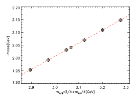
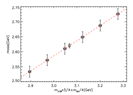
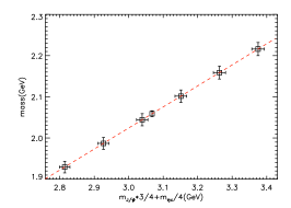
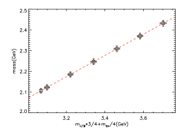
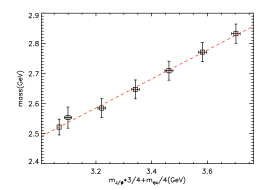
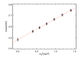
Let us first examine the mass of the $D^{*}$ and $D_{1}$ mesons. After obtaining the mass values for them under various quark mass parameters $(\kappa^{ud},\kappa^{c})$, the mass of the $\eta_{c}$ and $J/\Psi$ are used to fix the physical charm quark hopping parameter $\kappa^{c}$. For this purpose, we demand that the combination ${1\over 4}m_{\eta_{c}}+{3\over 4}m_{J/\psi}$ (spin-averaged charmonium mass) reproduces its physical value with the scale set by the lattice spacing. This procedure is shown in Fig. 1 where the mass values of $D^{*}$ and $D_{1}$ are shown as functions of the charm quark mass parameter $\kappa^{c}$. The left panel is for $D^{\ast}$, and the right one is for $D_{1}$. In each figure, the 6 data points with both $x$ and $y$ error-bars are original data for the $D$ meson mass. The interpolated point with only $y$ error-bar is the result of charm quark mass interpolation. Such interpolations are performed for each light quark mass parameter $\kappa^{ud}$ although in Fig. 1 one particular light quark mass parameter $\kappa^{ud}$ is shown.

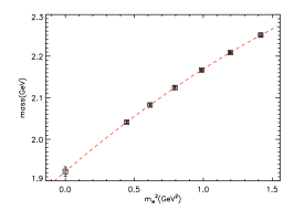
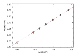
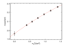
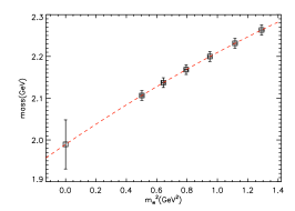
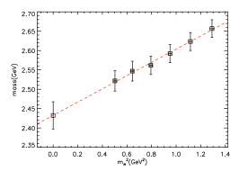
After heavy quark mass interpolation for each light quark mass parameter $\kappa^{ud}$, the mass of the $D^{*}$ and $D_{1}$ mesons ($m_{D^{\ast}}$ and $m_{D_{1}}$, respectively) are extrapolated versus $m_{\pi}^{2}$ towards the chiral limit $m^{2}_{\pi}=0$. Since our simulation points are still far from the true chiral region, we adopted either linear or quadratic functions in $m^{2}_{\pi}$ according to the behavior of the data. This procedure is shown in Fig. 2.

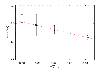
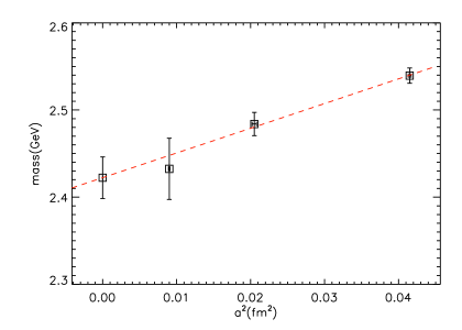
After all these interpolations and extrapolations, we obtain the mass of $D^{\ast}$ and $D_{1}$ for each lattice spacing. Finally, a continuum extrapolation can be carried out for $m_{D^{\ast}}$ and $m_{D_{1}}$ with linear function in $a^{2}_{s}$ since we are using an improved fermion action. This is illustrated in Fig. 3. Our final results for the mass of the $D$ mesons are:

$$m_{D^{\ast}}=2.008\pm 0.039{\rm GeV},~{}m_{D_{1}}=2.422\pm 0.024{\rm GeV},$$ (26)

from which we can see that our results are compatible with experimental result within error bars.

Let us now move on to the dispersion relations for $D^{*}$, $D_{1}$, $\eta_{c}$ and $J/\Psi$. The aim for this study is to verify that we do get single-particle asymptotic states. For this we need to know the energy of these particles with definite three-momentum. Since the correlators with non-zero three-momentum $C(t,{\bf k})$ is much noisier than the one with zero three-momentum $C(t,{\bf 0})$, it is difficult to obtain the plateau of the energy directly, particularly for the axial-vector meson $D_{1}$. To get around this, we form the following ratio:

$$R(t,{\bf k})={C(t,{\bf k})\over C(t,{\bf 0})}\propto e^{-\delta E({\bf k})\cdot t}$$ (27)

where $\delta E({\bf k})=E({\bf k})-E({\bf 0})$ designates the “kinetic energy” of the particle. It turns out that, by forming this ratio, most of the noise is suppressed and a plateau for $\delta E({\bf k})$ can be extracted from:

$$\delta E_{\rm eff.}({\mathbf{k}},t)=\log{R(t,{\bf k})\over R(t+1,{\bf k})}.$$ (28)

These plateaus are illustrated in Fig. 4. In fact, for the $D^{\ast}$, $J/\psi$ and $\eta_{c}$ mesons, we can also get the plateau directly. There is no need to form the ratio. However, if we do form the ratio, the results we get from this ratio are fully compatible with what we get by direct extraction from the original correlators. For the axial-vector meson $D_{1}$, however, forming the ratio helps to suppress the noise and to develop the mass plateau.

After getting the results of $\delta E({\bf k})$, the results for $E({\bf k})=E(0)+\delta E({\bf k})$ is also obtained from which one can check the dispersion relation at low-momenta:

$$E^{2}({\bf k})=m^{2}+Z\cdot{\bf k}^{2}+\cdots\;,$$ (29)

where $Z$ is a parameter to be fitted. In order to recover usual continuum dispersion relation with $Z=1$, one has to tune the bare speed of light parameter $\nu$ in the fermion action. This has been done in Ref. [24], for several values of $\beta$. In this study, we use the results of $\nu$ in Ref. [24] as input parameters. Since we have get the value of $E({\bf k})$ in our calculation, we can fit the our data using Eq. (29), and get the value of $Z$. As an illustration, the results of dispersion relations are shown in Fig. 5 for certain input quark mass parameters. The values of $Z$ are also indicated in each panel. From these results, it is seen that the values of $Z$ is approximately equal to 1 for $\eta_{c}$ and $J/\Psi$, which suggests that our choice for the value of $\nu$ is approximately right.

After all these checking, including the mass spectrum and the dispersion relations for the $D^{*}$ and $D_{1}$ mesons, we are confident that our finite box can accommodate well-established single-particle asymptotic states and we may now proceed to study the scattering of $D^{*}$ and $D_{1}$ mesons at low-momenta.

4.3 Results for the scattering length and effective range

As we argued in Sec. 3, only one correlation matrix $C(t)$ have to be computed for each symmetry channel of the two-particle system. For each symmetry channel, we have studied $5$ different non-zero momentum modes. Therefore, including the zero-momentum mode, for each symmetry channel, the correlation matrix for the two-particle system is a $6\times 6$ matrix.

To extract the two-particle energy eigenvalues, we adopt the usual ${\rm L\ddot{u}scher-Wolff}$ method [13]. For this purpose, a new matrix $\Omega(t,t_{0})$ is defined as:

$$\Omega(t,t_{0})=C(t_{0})^{-{1\over 2}}C(t)C(t_{0})^{-{1\over 2}},$$ (30)

where $t_{0}$ is a reference time-slice. Normally one picks a $t_{0}$ such that the signal is good and stable. The energy eigenvalues for the two-particle system are then obtained by diagonalizing the matrix $\Omega(t,t_{0})$. The $i$-th eigenvalue of the matrix has the following behavior in the large $(t-t_{0})$ limit:

$$\lambda_{i}(t,t_{0})\propto e^{-E_{i}(t-t_{0})}\;.$$ (31)

Therefore, the exact energy $E_{i}$ can be extracted from the effective mass plateau of the eigenvalue $\lambda_{i}$.

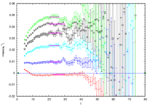
The real signal for the eigenvalue in our simulation turns out to be so noisy that reliable plateau cannot be found directly. Therefore, the following ratio was attempted:

$${\mathcal{R}}(t,t_{0})={\lambda_{i}(t,t_{0})\over C_{D^{\ast}}(t)C_{D_{1}}(t)}\propto e^{-\delta E_{i}\cdot t}$$ (32)

where $C_{D^{\ast}}(t)$ and $C_{D_{1}}(t)$ are one-particle correlation function with zero momentum for the corresponding mesons. Therefore, $\delta E_{i}$ is the difference of the two-particle energy with the threshold of the two mesons:

$$\delta E_{i}=E_{i}-m_{D^{\ast}}-m_{D_{1}}$$ (33)

By taking this ratio, the signal to noise ratio is greatly enhanced. The energy difference $\delta E_{i}$ can be extracted reliably from the following effective mass:

$$M_{\rm eff}(t)=\ln\left({{\mathcal{R}}(t)\over{\mathcal{R}}(t+1)}\right)\;.$$ (34)

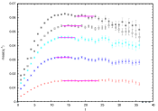
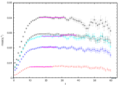
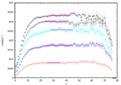
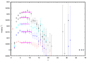
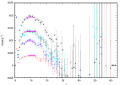
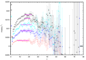
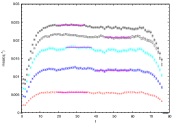
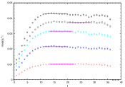
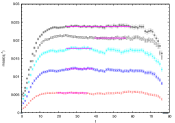
For the $A^{(1)}_{1}$ channel with correlation matrix given in Eq. (20), the situation is illustrated in Fig. 6 for lattices at $\beta=2.5$, $2.8$ and $3.2$. Six different plateaus in each panel correspond to different modes and this procedure is carried out for each pair of quark mass parameters $(\kappa^{ud},\kappa^{c})$.

With the energy difference $\delta E_{i}$ extracted from the simulation data, one utilizes the definition:

$$\sqrt{m_{D^{\ast}}^{2}+\bar{\bf k}^{2}}+\sqrt{m_{D_{1}}^{2}+\bar{\bf k}^{2}}=\delta E_{i}+m_{D^{\ast}}+m_{D_{1}}$$ (35)

to solve for $\bar{{\mathbf{k}}}^{2}$ which is then plugged into the modified Lüscher’s formula (i.e. Eq. (7). Close to the scattering threshold, the quantity $k/\tan\delta(k)$ has the following expansion:

$${k\over\tan\delta(k)}={1\over a_{0}}+{1\over 2}r_{0}k^{2}+\cdots\;,$$ (36)

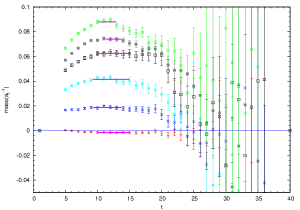
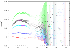
where $a_{0}$ is the scattering length and $r_{0}$ is the effective range. The l.h.s of Eq.(36) can also be calculated using Lüscher’s formula. Therefore, we can fit our data with Eq. (36), from which the values of $a_{0}$ and $r_{0}$ are obtained. Since Eq. (36) is only valid when $k$ is small, we use the data for the lowest $4$ modes in the fitting. For a particular choice of $(\kappa^{ud},\kappa^{c})$, this fitting procedure is shown in Fig. 7 for three values of $\beta$ in our simulation.

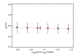
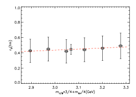
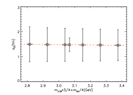
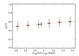
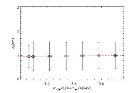
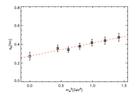
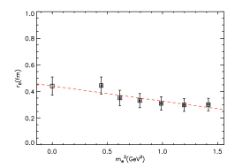
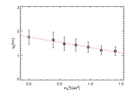
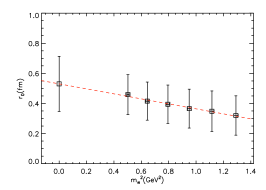
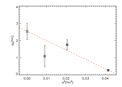
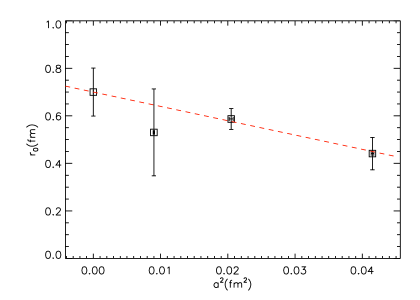
After getting the value of $a_{0}$ and $r_{0}$ for each pair of quark mass parameter $(\kappa^{ud},\kappa^{c})$, the results are interpolated versus $\kappa^{c}$ to the physical charm quark mass which is determined by the experimental value of ${1\over 4}m_{\eta_{c}}+{3\over 4}m_{J/\psi}$. This is shown in Fig. 8. The interpolated data are then taken for the chiral extrapolation. In this step, the results for $a_{0}$ and $r_{0}$ are extrapolated versus $m^{2}_{\pi}$ towards the chiral limit as shown in Fig. 9. Finally, continuum limit is taken by a linear extrapolation in $a^{2}_{s}$ for the results of $a_{0}$ and $r_{0}$ obtained after chiral extrapolation. The final results for the scattering length $a_{0}$ and the effective range $r_{0}$ in this channel is shown in figure 10. After these extrapolations, we obtain the scattering length $a_{0}$ and the effective range $r_{0}$ for the $A_{1}$ channel:

$$a_{0}=2.53\pm 0.47{\rm fm},~{}r_{0}=0.70\pm 0.10{\rm fm}\;.$$ (37)

This result is for $A^{(1)}_{1}$ channel which, in the notion of continuum quantum numbers, corresponds to $J^{P}=0^{-}$. The signal in other channels is much noisier than that of $A^{(1)}_{1}$ channel and it seems that more statistics and/or better interpolation operators are needed for a reliable extraction of the scattering parameters. Results for the scattering length $a_{0}$ and the effective range $r_{0}$ at various light quark mass parameters for three values of $\beta$ are also listed in Table 4 for reference. The results after the chiral extrapolations and the final results in the continuum limit are also shown in the table.

4.4 Possibility of a shallow bound state

$\beta$	$q^{2}$	$\cot\sigma(q^{2})$
2.5	-0.026(0.003)	5.23(0.65)
2.8	-0.064(0.005)	0.16(0.18)
3.2	-0.053(0.016)	0.92(0.93)

Table 3: Results for the lowest $q^{2}$ and the corresponding values for $\cot\sigma(q)$ as given by Eq. (8) for different values of $\beta$ in the simulation. Corresponding errors for the quantities are also given in the parenthesis.

To explore the possibility of a bound state, we recall that for a bound state to exist, $q^{2}$ has to be negative and in fact $q^{2}\rightarrow-\infty$ as $L\rightarrow\infty$. This results in the condition: $\cot\sigma(q)=-1$ as discussed in the subsection 2.1, Eq. (8). On the other hand, a scattering state will have: $q^{2}\simeq(1/L)$ as $L\rightarrow\infty$. Results for the lowest (negative) $q^{2}$ and the corresponding values of $\cot\sigma(q)$ as computed from Eq. (8) are listed in Table 3. It is seen that our results for $\cot\sigma(q)$ for the lowest (negative) $q^{2}$ are all positive. The absolute values for the lowest $q^{2}$ are also not large. Our results obtained so far seems to be more consistent with a scattering state than a bound state.

One could investigate this possibility from another point of view, namely by the values of scattering length and effective range. The value of effective range $r_{0}$ obtained is much less than the size of our box so that using Lüscher’s formalism is justified. Since we are studying the scattering near the threshold, it is appropriate to study the problem using non-relativistic quantum mechanics. Within non-relativistic quantum mechanics, it is known that, if a shallow bound state emerges in $s$-wave potential scattering at low-energies, the scattering length of the system will diverge. In fact, if the potential acquires an infinitely shallow bound state, the scattering length should approach negative infinity [16]. Our lattice results for the scattering lengths indicate that it is quite large but positive. This usually happens when the potential is on the verge of developing a shallow bound state. Note that this argument is generally valid for a wide variety of potentials.

If we further approximate the potential by a square-well potential, we could even estimate the depth $V_{0}$ and the range of the potential $R$ from our lattice results on $a_{0}$ and $r_{0}$. We find that, $R=r_{0}=0.70(10)$fm and $V_{0}=73(21)$MeV. These values for a square-well potential also gives no bound states. If we fix $r_{0}R=0.7$fm, the first bound state will occur at about $V_{0}\simeq 92$MeV.

5 Conclusions

In this paper, we present our quenched anisotropic lattice study for the scattering of $D^{*}$ and $D_{1}$ mesons near the threshold. The calculation is based on a finite-size technique due to Lüscher which enables us to extract the scattering phases from the exact two-particle energies measured in Monte Carlo simulations. Our study focuses on the $s$-wave scattering in the channel $J^{P}=0^{-}$ and the scattering threshold parameters, i.e. scattering length $a_{0}$ and effective range $r_{0}$ are obtained. After the chiral and continuum extrapolations, we obtain: $a_{0}=2.53(47)$fm and $r_{0}=0.70(10)$fm, indicating that the interaction between a $D^{*}$ and a $D_{1}$ meson is attractive in this channel. As for the other channels, although we have also computed the correlation matrices, but the signal is too noisy to obtain definite results. Better operators and more statistics are probably needed in further studies.

Based on our results for the scattering phases near the threshold, we have also discussed the possibility of a shallow bound state in this channel. We investigate the quantity $\cot\sigma$ which should approach $(-1)$ for a bound state. Our results for this quantity are all positive. Our results for scattering length are also positive. Based on these indications, it seems that, although the interaction between the two charmed mesons is attractive, it is unlikely that they form a genuine bound state right below the threshold. The lowest two-particle state is likely to be a scattering state. This result might shed some light on the nature of the recently discovered $Z^{+}(4430)$ state by Belle. However, we should emphasize that, our lattice calculation is done in a particular channel only and it is within the quenched approximation. Obviously, to further clarify the nature of the structure $Z^{+}(4430)$, lattice studies in other symmetry channels and preferably with dynamical fermions are much welcomed.

References

- [1] S. K. Choi et al. Observation of a resonance-like structure in the mass distribution in exclusive decays. Phys. Rev. Lett., 100:142001, 2008.
- [2] Jonathan L. Rosner. Threshold effect and peak. Phys. Rev., D76:114002, 2007.
- [3] Xiang Liu, Yan-Rui Liu, Wei-Zhen Deng, and Shi-Lin Zhu. Is a loosely bound molecular state? Phys. Rev., D77:034003, 2008.
- [4] Xiang Liu, Yan-Rui Liu, Wei-Zhen Deng, and Shi-Lin Zhu. as a () molecular state. Phys. Rev., D77:094015, 2008.
- [5] D. V. Bugg. How Resonances can synchronise with Thresholds. J. Phys., G35:075005, 2008.
- [6] Cong-Feng Qiao. A Uniform Description of the States Recently Observed at B-factories. J. Phys., G35:075008, 2008.
- [7] Su Houng Lee, Antonio Mihara, Fernando S. Navarra, and Marina Nielsen. QCD sum rules study of the meson . Phys. Lett., B661:28–32, 2008.
- [8] Eric Braaten and Meng Lu. Line Shapes of the Z(4430). Phys. Rev., D79:051503, 2009.
- [9] Xiao-Hai Liu, Qiang Zhao, and Frank E. Close. Search for tetraquark candidate in meson photoproduction. Phys. Rev., D77:094005, 2008.
- [10] Stephen Godfrey and Stephen L. Olsen. The Exotic XYZ Charmonium-like Mesons. Ann. Rev. Nucl. Part. Sci., 58:51–73, 2008.
- [11] M. Lüscher. Volume dependence of the energy spectrum in massive quantum field theories. 1. stable particle states. Commun. Math. Phys., 104:177, 1986.
- [12] M. Lüscher. Volume dependence of the energy spectrum in massive quantum field theories. 2. scattering states. Commun. Math. Phys., 105:153, 1986.
- [13] M. Lüscher and U. Wolff. How to calculate the elastic scattering matrix in two-dimensional quantum field theories by numerical simulation. Nucl. Phys. B, 339:222, 1990.
- [14] M. Lüscher. Two particle states on a torus and their relation to the scattering matrix. Nucl. Phys. B, 354:531, 1991.
- [15] M. Lüscher. Signatures of unstable particles in finite volume. Nucl. Phys. B, 364:237, 1991.
- [16] Shoichi Sasaki and Takeshi Yamazaki. Identification of shallow two-body bound states in finite volume. PoS, LAT2007:131, 2007.
- [17] X. Li and C. Liu. Two particle states in an asymmetric box. Phys. Lett. B, 587:100, 2004.
- [18] X. Feng, X. Li, and C. Liu. Two particle states in an asymmetric box and the elastic scattering phases. Phys. Rev. D, 70:014505, 2004.
- [19] Xin Li et al. Hadron Scattering in an Asymmetric Box. JHEP, 06:053, 2007.
- [20] C. Morningstar and M. Peardon. The glueball spectrum from an anisotropic lattice study. Phys. Rev. D, 60:034509, 1999.
- [21] C. Liu. A lattice study of the glueball spectrum. Chinese Physics Letter, 18:187, 2001.
- [22] Y. Chen, A. Alexandru, S.J. Dong, T. Draper, I. Horvath, F.X. Lee, K.F. Liu, N. Mathur, C. Morningstar, M. Peardon, S. Tamhankar, B.L. Young, and J.B. Zhang. Glueball spectrum and matrix elements on anisotropic lattices. Phys. Rev. D, 73:014516, 2006.
- [23] Junhua Zhang and C. Liu. Tuning the tadpole improved clover wilson action on coarse anisotropic lattices. Mod. Phys. Lett. A, 16:1841, 2001.
- [24] Shiquan Su, Liuming Liu, Xin Li, and Chuan Liu. A numerical study of improved quark actions on anisotropic lattices. Int. J. Mod. Phys. A, 21:1015, 2006.
- [25] U. Glaessner, S. Guesken, T. Lippert, G. Ritzenhoefer, K. Schilling, and A. Frommer. How to compute green’s functions for entire mass trajectories within krylov solvers. hep-lat/9605008.
- [26] Wei Liu, Ying Chen, Ming Gong, Xin Li, GuoZhan Meng, and Chuan Liu. Static quark potential and the renormalized anisotropy on tadpole improved anisotropic lattices. Mod. Phys. Lett. A, 21:2313, 2006.