Bounds on the width, mass difference and other properties of $X(3872)\rightarrow\pi^{+}\pi^{-}J/\psi$ decays

Abstract

We present results from a study of $X(3872)\rightarrow\pi\pi J/\psi$ decays produced via exclusive $B\rightarrow KX(3872)$ decays. We determine the mass to be $M_{X(3872)}=(3871.84\pm 0.27{\rm(stat)}\pm 0.19~{}{\rm(syst)})$ MeV, a 90% CL upper limit on the natural width of $\Gamma_{X(3872)}<1.2$ MeV, the product branching fraction ${\mathcal{B}}(B^{+}\rightarrow K^{+}X(3872))\times{\mathcal{B}}(X(3872)\rightarrow\pi^{+}\pi^{-}J/\psi)=(8.61\pm 0.82~{}{\rm(stat)}\pm 0.52~{}{\rm(syst)})\times 10^{-6}$, and a ratio of branching fractions ${\mathcal{B}}(B^{0}\rightarrow K^{0}X(3872))/{\mathcal{B}}(B^{+}\rightarrow K^{+}X(3872))=0.50\pm 0.14~{}{\rm(stat)}\pm 0.04~{}{\rm(syst)}.$ The difference in mass between the $X(3872)\rightarrow\pi^{+}\pi^{-}J/\psi$ signals in $B^{+}$ and $B^{0}$ decays is $\Delta M_{X(3872)}=(-0.69\pm 0.97{\rm(stat)}\pm 0.19{\rm(syst)})$ MeV. A search for a charged partner of the $X(3872)$ in the decays $\bar{B}^{0}\rightarrow K^{-}X^{+}$ or $B^{+}\rightarrow K^{0}X^{+}$, $X^{+}\rightarrow\pi^{+}\pi^{0}J/\psi$ resulted in upper limits on the product branching fractions for these processes that are well below expectations for the case that the $X(3872)$ is the neutral member of an isospin triplet. In addition, we examine possible $J^{PC}$ quantum number assignments for the $X(3872)$ based on comparisons of angular correlations between final state particles in $X(3872)\rightarrow\pi^{+}\pi^{-}J/\psi$ decays with simulated data for $J^{PC}$ values of $1^{++}$ and $2^{-+}$. We examine the influence of $\rho$-$\omega$ interference in the $M(\pi^{+}\pi^{-})$ spectrum. The analysis is based on a 711 fb^-1 data sample that contains 772 million $B\bar{B}$ meson pairs collected at the $\Upsilon(4S)$ resonance in the Belle detector at the KEKB $e^{+}e^{-}$ collider.

I Introduction

The $X(3872)$ was first observed by Belle as a narrow peak in the $\pi^{+}\pi^{-}J/\psi$ invariant mass distribution in exclusive $B^{+}\rightarrow K^{+}\pi^{+}\pi^{-}J/\psi$ decays skchoi_x3872 ; conj . It was subsequently seen in $\sqrt{s}=1.96$ TeV $p\bar{p}$ annihilations by CDF CDF_x3872 and D0 D0_x3872 and its production in $B$ decays was confirmed by BaBar babar_x3872 . A recent summary of the measured properties of the $X(3872)$ is provided in Tables 10 through 13 of Ref. brambilla .

The close proximity of the PDG world-average of $X(3872)$ mass measurements, $M_{\rm avg}=3871.56\pm 0.22$ MeV PDG , to the $m_{D^{0}}+m_{\bar{D}^{*0}}$ mass threshold ($3871.8\pm 0.3$ MeV PDG ) has engendered speculation that the $X(3872)$ might be a loosely bound $D^{0}$-$\bar{D}^{*0}$ molecular state molecule . Theoretical studies of deuteron-like $D^{0}\bar{D}^{*0}$ interactions were reported by Törnqvist in 1994, and he predicted bound states for $J^{PC}$ values of $0^{-+}$ and $1^{++}$ tornqvist_1994 . There has been considerable theoretical interest in the $X(3872)$ line shape in its $D^{0}\bar{D}^{*0}$ decay mode x3872_lineshape . These discussions are constrained by the current uncertainty in the natural width of the $X(3872)$ in the $\pi^{+}\pi^{-}J/\psi$ decay channel, which is $\Gamma_{X(3872)}<2.3$ MeV (at the 90% confidence level) skchoi_x3872 . A measurement of the natural width in this mode, or an improvement in the upper limit on its value, would be useful input to these line-shape studies.

A close correspondence of the $\pi^{+}\pi^{-}$ invariant mass distribution to expectations for $\rho\rightarrow\pi^{+}\pi^{-}$ decays was reported by Belle belle_pipi and CDF cdf_pipi . This, together with the observation of the $X(3872)\rightarrow\gamma J/\psi$ decay mode by both Belle vishnal_qwg7 and BaBar babar_gampsi , establishes the charge parity of the $X(3872)$ as $C=+1$. A comprehensive study of possible $J^{PC}$ quantum numbers for the $X(3872)$ using a large sample of $X(3872)\rightarrow\pi^{+}\pi^{-}J/\psi$ decays was performed by CDF CDF_angles ; heuser_thesis ; they concluded that only the $1^{++}$ and $2^{-+}$ hypotheses are consistent with data and other assignments are ruled out at the $3\sigma$ level or above. The $X(3872)\rightarrow\gamma J/\psi$ decay process would be an allowed $E1$ transition for a $1^{++}$ assignment and a suppressed higher multipole for $2^{-+}$; the observation by BaBar and Belle of this process favors $1^{++}$ m2 . However, a recent BaBar analysis of the $X(3872)\rightarrow\pi^{+}\pi^{-}\pi^{0}J/\psi$ decay mode showed some preference for a $2^{-+}$ assignment babar_3pijpsi . Since bound molecular states are predicted for $J^{PC}=1^{++}$ but not for $2^{-+}$, an unambiguous experimental determination of the spin-parity of the $X(3872)$ is an important input to the understanding of this state.

Another proposed interpretation for the $X(3872)$ is that it is a tightly bound diquark-diantiquark four-quark state maiani , in which case two neutral $X(3872)$ states – orthogonal mixtures of $cu\bar{c}\bar{u}$ and $cd\bar{c}\bar{d}$ – are expected to exist shifted in mass by $8\pm 3$ MeV. The authors of Ref. maiani suggested that these two different states might result in different $X(3872)$ masses in the $B^{+}\rightarrow K^{+}\pi^{+}\pi^{-}J/\psi$ and $B^{0}\rightarrow K^{0}\pi^{+}\pi^{-}J/\psi$ decay chains. BaBar measured the $X(3872)$ properties separately for these two channels and found a mass difference ($\Delta M=2.7\pm 1.6\pm 0.4$ MeV) that is consistent both with zero and the lower range of the theoretical prediction babar_pipijpsi . CDF used a comparison of their measured $X(3872)\rightarrow\pi^{+}\pi^{-}J/\psi$ line width with their experimental resolution to establish a 95% CL upper limit of $\Delta M<3.6$  MeV, for equal production of the two states cdf_pipijpsi . These results are not definitive tests of the prediction of Ref. maiani ; the statistical significance of the BaBar signal for $B^{0}\rightarrow K^{0}X(3872)$ is marginal ($9.4\pm 5.2$ events) and the interpretation of the CDF limit depends upon the unknown relative production strengths for the two different states. Thus, a more precise comparison of the $X(3872)$ produced in $B^{+}$ and $B^{0}$ decays is needed.

In the diquark-diantiquark scheme, the $X(3872)$ is expected to be the $I_{3}=0$ member of an isospin triplet. Since the dominant weak interaction process responsible for $B\rightarrow KX(3872)$ decays is the isospin conserving $b\rightarrow c\bar{c}s$ transition, the charged $I_{3}=\pm 1$ partner states (that decay via $X^{+}\rightarrow\rho^{+}J/\psi$) are expected to be produced in $B$ decays at a rate that is twice that for the neutral $X(3872)$ braaten . The BaBar group studied the process $B\rightarrow K\pi^{+}\pi^{0}J/\psi$ and placed upper limits on the product branching fractions for $X^{+}\rightarrow\pi^{+}\pi^{0}J/\psi$ that are below isospin expectations babar_pipi0jpsi .

Here we report on a study of $X(3872)\rightarrow\pi^{+}\pi^{-}J/\psi$ decays produced via the exclusive decay $B\rightarrow KX(3872)$. We use a 711 fb^-1 data sample that contains 772 million $B\bar{B}$ pairs collected in the Belle detector at the KEKB energy-asymmetric $e^{+}e^{-}$ collider full_data . The data were accumulated at a center-of-mass system (cms) energy of $\sqrt{s}=10.58$ GeV, at the peak of the $\Upsilon(4S)$ resonance. KEKB is described in detail in Ref. KEKB .

II Detector description

The Belle detector is a large-solid-angle magnetic spectrometer that consists of a silicon vertex detector (SVD), a 50-layer cylindrical drift chamber (CDC), an array of aerogel threshold Cherenkov counters (ACC), a barrel-like arrangement of time-of-flight scintillation counters (TOF), and an electromagnetic calorimeter (ECL) comprised of CsI(Tl) crystals located inside a superconducting solenoid coil that provides a 1.5 T magnetic field. An iron flux-return located outside of the coil is instrumented to detect $K_{L}$ mesons and to identify muons (KLM). The detector is described in detail elsewhere Belle .

III $B\rightarrow K\pi^{+}\pi^{-}J/\psi$ event selection

We select events that contain a $J/\psi\rightarrow\ell^{+}\ell^{-}$ ($\ell^{+}\ell^{-}=e^{+}e^{-}$ or $\mu^{+}\mu^{-}$), either a charged or neutral kaon, and a $\pi^{+}\pi^{-}$ pair using criteria described in Refs skchoi_x3872 and skchoi_y3940 . The leptons from the $J/\psi\rightarrow\ell^{+}\ell^{-}$ decay are required to pass minimal lepton identification criteria and the invariant mass of the pair is required to be in the ranges $-21$ MeV $\leq(M_{\mu^{+}\mu^{-}}-m_{J/\psi})\leq 20$ MeV and $-24$ MeV $\leq(M_{e^{+}e^{-}}-m_{J/\psi})\leq 20$ MeV, where $m_{J/\psi}=3096.92\pm 0.01$ MeV is the world-average value for the $J/\psi$ mass PDG . For $J/\psi\rightarrow e^{+}e^{-}$ candidates, photons within 50 mrad of the $e^{+}$ and/or $e^{-}$ tracks are included in the invariant mass calculation. The number of events with multiple $J/\psi$ candidates is negligibly small. Candidate $K^{+}$ mesons are charged tracks with a kaon identification likelihood that is higher than that for a pion or a proton; neutral kaons are detected in the $K_{S}\rightarrow\pi^{+}\pi^{-}$ decay channel using the $K_{S}$ selection criteria described in Ref. belle_ffang . The charged pions are required to have a pion likelihood greater than that of a kaon or a proton. Some events have more than one acceptable combination of hadron tracks. In these cases, which include 3% of the events in the signal region, the tracks with the best vertex fits are used. To reduce the level of $e^{+}e^{-}\rightarrow q\bar{q}$ ($q=u,d,s~{}{\rm or}~{}c$-quark) continuum events in the sample, we also require $R_{2}<0.4$, where $R_{2}$ is the normalized Fox-Wolfram moment fox .

Events that originate from $B\rightarrow K\pi^{+}\pi^{-}J/\psi$ decays are identified by the cms energy difference $\Delta E\equiv E_{B}^{\rm cms}-E_{\rm beam}^{\rm cms}$ and the beam-energy-constrained mass $M_{\rm bc}\equiv\sqrt{(E_{\rm beam}^{\rm cms})^{2}-(p_{B}^{\rm cms})^{2}}$, where $E_{\rm beam}^{\rm cms}$ is the cms beam energy, and $E_{B}^{\rm cms}$ and $p_{B}^{\rm cms}$ are the cms energy and momentum of the $K\pi^{+}\pi^{-}J/\psi$ combination. We select events with $M_{\rm bc}>5.20$ GeV and $-0.15~{}{\rm GeV}<\Delta E<0.2$ GeV. We define signal regions as $5.272~{}{\rm GeV}<M_{\rm bc}<5.286$ GeV and $-0.35\,\mathrm{GeV}\leq\Delta E\leq 0.03\,\mathrm{GeV}$; these correspond to $\simeq\pm 2.5\sigma$ windows around the central values for each variable.

In addition to selecting $B\rightarrow KX(3872)$ events, these selection criteria isolate a rather pure sample of $B\rightarrow K\psi^{\prime}$, $\psi^{\prime}\rightarrow\pi^{+}\pi^{-}J/\psi$ events psiprime . These events are used as a calibration reaction to determine the $M_{\rm bc}$, $\Delta E$ and $M(\pi^{+}\pi^{-}J/\psi)$ peak positions and resolution values, and to validate the Monte Carlo-determined acceptance calculations.

For each event we compute $M(\pi^{+}\pi^{-}J/\psi)$ from the relation

$$M(\pi^{+}\pi^{-}J/\psi)=M^{\rm meas}_{\pi^{+}\pi^{-}\ell^{+}\ell^{-}}-M^{\rm meas}_{\ell^{+}\ell^{-}}+m_{J/\psi},$$ (1)

where $M^{\rm meas}_{\pi^{+}\pi^{-}\ell^{+}\ell^{-}}$ and $M^{\rm meas}_{\ell^{+}\ell^{-}}$ are the measured $\pi^{+}\pi^{-}\ell^{+}\ell^{-}$ and $\ell^{+}\ell^{-}$ invariant masses, respectively. For studies of the $\psi^{\prime}\rightarrow\pi^{+}\pi^{-}J/\psi$ control sample we use events in the interval $3.635~{}{\rm GeV}\leq M(\pi^{+}\pi^{-}J/\psi)\leq 3.735$ GeV; for $X(3872)$ studies we use $3.77~{}{\rm GeV}\leq M(\pi^{+}\pi^{-}J/\psi)\leq 3.97$ GeV. The $M(\pi^{+}\pi^{-}J/\psi)$ signal regions are defined as $|M(\pi^{+}\pi^{-}J/\psi)-M_{\rm peak}|\leq 0.009$ GeV, where $M_{\rm peak}=3.686$ GeV and $3.872$ GeV for the $\psi^{\prime}$ and $X(3872)$, respectively. We select events with a dipion invariant mass requirement of $M_{\pi^{+}\pi^{-}}>(M(\pi^{+}\pi^{-}J/\psi)-(m_{J/\psi}+150~{}{\rm MeV}))$, which corresponds to $M_{\pi^{+}\pi^{-}}>625$ MeV for the $X(3872)$ and $>439$ MeV for the $\psi^{\prime}$ events. After this requirement, which results in a 6% signal loss, the background under the $X(3872)\rightarrow\pi^{+}\pi^{-}J/\psi$ signal peak is relatively flat and similar in shape to that under the $\psi^{\prime}\rightarrow\pi^{+}\pi^{-}J/\psi$ peak.

IV Monte Carlo results

We use Monte Carlo (MC) simulated events to determine acceptance and to evaluate possible differences in mass biases for the $\psi^{\prime}$ and $X(3872)$ mass regions geant . The $\psi^{\prime}$ MC simulation uses an input mass and width of: $m_{\psi^{\prime}}=3686.09$ MeV and $\Gamma_{\psi^{\prime}}=0.3$ MeV PDG . The default $X(3872)$ simulation assumes $J^{PC}=1^{++}$ and a $\pi^{+}\pi^{-}J/\psi$ final state that is entirely $B\rightarrow\rho J/\psi$ with the $\rho$ and $J/\psi$ in a relative $S$-wave evtgen . The $X(3872)$ mesons are generated with a mass of $M^{\rm gen}_{X(3872)}=3871.40$ MeV and zero natural width. The simulated events are processed through the same reconstruction and selection codes that are used for the real data.

We perform an unbinned three-dimensional likelihood fit ($M_{\rm bc}$ vs. $M(\pi^{+}\pi^{-}J/\psi)$ vs. $\Delta E$) to the selected data using a single Gaussian function for the $M_{\rm bc}$ signal probability density function (PDF) and an ARGUS function ARGUS as the PDF for the combinatorial background (i.e., backgrounds where one or more of the tracks used to reconstruct the $B$ originates from the accompanying $\bar{B}$). For $\Delta E$ we use a bifurcated Gaussian for the signal PDF and a second-order polynomial for the $\Delta E$ combinatorial background. For the $M(\pi^{+}\pi^{-}J/\psi)$ signal PDF we use a Breit-Wigner function (BW) convolved with a resolution function that is the sum of a core and tail Gaussian; for the combinatorial background PDF we use a third-order polynomial. For $\psi^{\prime}$ fits in both data and MC, we fix the BW width at $0.3$ MeV. For the $X(3872)$ MC fits, we fix the BW width at zero.

In addition to combinatorial background, these criteria select events of the type $B\rightarrow K_{X}J/\psi$, where $K_{X}$ designates strange meson systems that decay to $K\pi^{+}\pi^{-}$ final states such as the $K_{1}(1270)$, $K_{2}^{*}(1430)$, etc. hulya . The $M_{\rm bc}$ and $\Delta E$ distributions for these events are the same as those of the $X(3872)$ signal, but they produce a slowly varying $M(\pi^{+}\pi^{-}J/\psi)$ distribution in the $\psi^{\prime}$ and $X(3872)$ signal regions. The $M_{\rm bc}$ and $\Delta E$ PDFs that are used to represent this peaking background are the same as those used for the signal and a linear form is used for its $M(\pi^{+}\pi^{-}J/\psi)$ PDF.

The results of fits to MC samples of $B^{+}\rightarrow K^{+}\psi^{\prime}$, $B^{0}\rightarrow K_{S}\psi^{\prime}$, $B^{+}\rightarrow K^{+}X(3872)$ and $B^{0}\rightarrow K_{S}X(3872)$ are summarized in Table 1. In order to facilitate comparisons of the resolution for different decay channels, the relative fraction of the tail and core Gaussian for all modes is fixed at the value returned from the fit to the $K^{+}\psi^{\prime}$ MC sample (17.7%). This restriction is found to induce negligible differences from the shapes of the resolution functions that are individually optimized for the other samples. While the core resolution width is nearly the same for all channels, the tail resolution widths for $X(3872)$ decays are significantly higher than those for the $\psi^{\prime}$, but in both cases the tail widths for the $K^{+}$ and $K_{S}$ modes are consistent with being the same. The MC indicates that there are biases in the $M(\pi^{+}\pi^{-}J/\psi)$ measurement that are smaller for the $X(3872)$ modes than for the $\psi^{\prime}$ modes. These are due to a bias in the measurement of the low momentum charged pions. The pions from $X(3872)$ decays have, on average, higher momentum than those from $\psi^{\prime}$ decays and the $X(3872)$ mass measurement bias is smaller. In both cases, the mass measurement biases for the $K^{+}$ and $K_{S}$ modes are consistent with being the same. The results of fits to the combined $K^{+}$ and $K_{S}$ modes are also shown in Table 1. (The listed efficiencies do not include the $\psi^{\prime}\rightarrow\pi^{+}\pi^{-}J/\psi$, $J/\psi\rightarrow\ell^{+}\ell^{-}$ or $K_{S}\rightarrow\pi^{+}\pi^{-}$ branching fractions).

Table 1: Results from fits to the selected MC event samples. Here $\epsilon=N_{\rm sig}/N_{\rm gen}$ is the detection efficiency, $\sigma_{\rm core}$ and $\sigma_{\rm tail}$ are the widths of the core and tail components of the mass resolution and $M_{\rm gen}-M_{\rm fit}$ are the MC mass measurement biases. All errors are statistical.

Channel	$\epsilon$	$\sigma_{\rm core}$	$\sigma_{\rm tail}$	$M_{\rm gen}-M_{\rm fit}$
	(percent)	(MeV)	(MeV)	(MeV)
$K^{+}\psi^{\prime}$	$17.8\pm 0.2$	$1.83\pm 0.02$	$5.66\pm 0.14$	$0.74\pm 0.02$
$K_{S}\psi^{\prime}$	$14.1\pm 0.2$	$1.83\pm 0.03$	$6.10\pm 0.21$	$0.74\pm 0.03$
Combined		$1.84\pm 0.02$	$5.66\pm 0.13$	$0.72\pm 0.02$
$K^{+}X(3872)$	$19.1\pm 0.2$	$1.93\pm 0.04$	$7.69\pm 0.17$	$0.60\pm 0.02$
$K_{S}X(3872)$	$15.2\pm 0.2$	$1.89\pm 0.02$	$7.64\pm 0.21$	$0.64\pm 0.02$
Combined		$1.93\pm 0.02$	$7.70\pm 0.15$	$0.60\pm 0.02$

V Fits to the $\psi^{\prime}\rightarrow\pi^{+}\pi^{-}J/\psi$ data samples

For fits to the $\psi^{\prime}$ data we fix the BW width at $0.3$ MeV and allow the core and tail widths of the $M(\pi^{+}\pi^{-}J/\psi)$ resolution function to vary as free parameters. The results of the fits to $B^{+}\rightarrow K^{+}\psi^{\prime}$ ($B^{0}\rightarrow K_{S}\psi^{\prime}$) are the smooth curves in the upper (lower) panels of Fig. 1, where $M_{\rm bc}$, $M(\pi^{+}\pi^{-}J/\psi)$ and $\Delta E$ distributions for events within the signal regions of the other two quantities are shown. In each panel, the combinatorial background is shown as a (red) dotted line, the combinatorial plus peaking background is shown as a (green) dashed line and the total background plus signal is shown as a (blue) solid line. The fit results are summarized in Table 2. They show a mass bias, i.e., a difference between the fitted mass and the PDG world-average value for $m_{\psi^{\prime}}$, that is larger than the MC mass bias, indicating that the MC simulation of the bias in the pion momentum measurement is imperfect.

Table 2: Results from fits to the $\psi^{\prime}$ event candidates. Here $N^{\rm evts}$ denotes the number of signal events returned from the fit, $\sigma_{\rm core}$ and $\sigma_{\rm tail}$ are the mass resolution parameters, and $\Delta M_{\rm PDG}=M_{\rm PDG}-M_{\rm fit}$ denotes the mass measurement biases. All errors are statistical.

Channel	$N^{\rm evts}$	$\sigma_{\rm core}$	$\sigma_{\rm tail}$	$\Delta M_{\rm PDG}$
		(MeV)	(MeV)	(MeV)
$K^{+}\psi^{\prime}$	$3575\pm 64$	$2.25\pm 0.05$	$8.4\pm 0.5$	$1.12\pm 0.05$
$K_{S}\psi^{\prime}$	$814\pm 30$	$2.45\pm 0.11$	$13.8\pm 1.6$	$1.05\pm 0.12$
Combined	$4367\pm 72$	$2.28\pm 0.04$	$8.7\pm 0.5$	$1.11\pm 0.05$

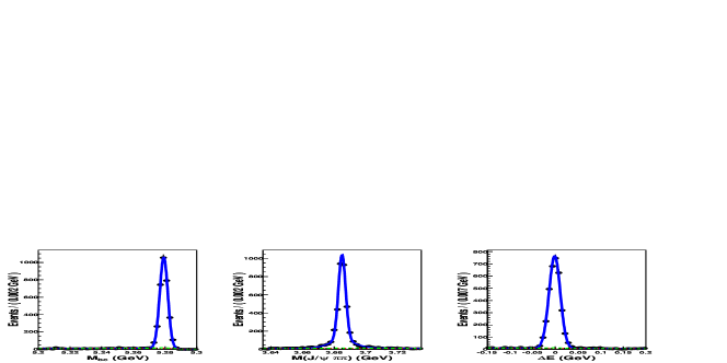
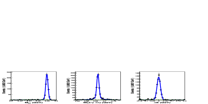
Figure 1: The $M_{\rm bc}$ (left), $M(\pi^{+}\pi^{-}J/\psi)$ (center) and $\Delta E$ (right) distributions for $B^{+}\rightarrow K^{+}\psi^{\prime}$ (top) and $B^{0}\rightarrow K_{S}\psi^{\prime}$ (bottom) event candidates within the signal regions of the other two quantities. The curves show the results of the fits described in the text.

As a test of the validity of the MC acceptance calculations, we determine branching fractions for $B\rightarrow K^{+}\psi^{\prime}$ and $K_{S}\psi^{\prime}$ via the relation

$${\mathcal{B}}(B\rightarrow K\psi^{\prime})=\frac{N^{\rm evts}_{K}}{N_{B\bar{B}}{\epsilon_{K}f_{K}{\mathcal{B}}_{\psi^{\prime}\rightarrow\pi^{+}\pi^{-}J/\psi}\mathcal{B}}_{J/\psi\rightarrow\ell\ell}},$$ (2)

where $N^{\rm evts}_{K}$ is the number of signal events for $K=K^{+}$ and $K=K^{0}$, $N_{B\bar{B}}=(772\pm 11)\times 10^{6}$ is the number of $B\bar{B}$ events in the data sample, ${\mathcal{B}}_{\psi^{\prime}\rightarrow\pi^{+}\pi^{-}J/\psi}=0.336\pm 0.004$ and ${\mathcal{B}}_{J/\psi\rightarrow\ell\ell}=0.119\pm 0.001$ (sum of the $e^{+}e^{-}$ and $\mu^{+}\mu^{-}$ modes) are PDG world-average branching fractions PDG , $\epsilon_{K}$ is the efficiency for the corresponding $K$ channel, $f_{K^{+}}=1$ and $f_{K_{S}}=0.346$ fks . The results are: ${\mathcal{B}}(B^{+}\rightarrow K^{+}\psi^{\prime})=(6.51\pm 0.12)\times 10^{-4}$ and ${\mathcal{B}}(B^{0}\rightarrow K^{0}\psi^{\prime})=(5.22\pm 0.19)\times 10^{-4}$, where only statistical errors are shown. The $B^{+}$ branching fraction result agrees well with the PDG world-average value of $(6.46\pm 0.33)\times 10^{-4}$. The $B^{0}$ result is somewhat lower than the PDG value of ($6.2\pm 0.5)\times 10^{-4}$ PDG , however, the errors quoted on the measurements reported here do not include systematic uncertainties.

VI $X(3872)\rightarrow\pi^{+}\pi^{-}J/\psi$ mass, width and product branching fractions

The upper panels in Fig. 2 show the $M_{\rm bc}$, $M(\pi^{+}\pi^{-}J/\psi)$ and $\Delta E$ distributions for events within the signal regions of the other two quantities for the $B^{+}\rightarrow K^{+}X(3872)$ event candidates together with the results of the fit. In these fits, the peak mass and full width of the BW function that represents the $M(\pi^{+}\pi^{-}J/\psi)$ signal are free parameters, the width of the core Gaussian resolution function is fixed at $\sigma_{\rm core}=2.28$ MeV, the measured $\psi^{\prime}$ core resolution value, and the width of the tail Gaussian is fixed at $\sigma_{tail}=11.5$ MeV, the tail width from the $\psi^{\prime}$ data sample fit multiplied by the ratio of the MC-determined $X(3872)$ and $\psi^{\prime}$ tail widths to account for its $M(\pi^{+}\pi^{-}J/\psi)$ dependence. The value for $\Gamma_{X(3872)}$ returned from the fit is at its lowest allowed value of $0.1$ MeV lower_limit . Other results from the fit are summarized in Table 3.

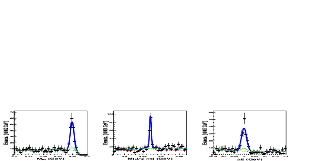
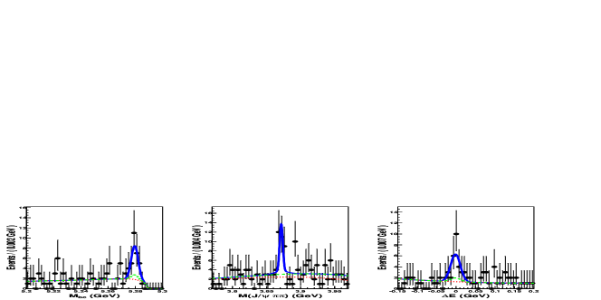
Figure 2: The $M_{\rm bc}$ (left), $M(\pi^{+}\pi^{-}J/\psi)$ (center) and $\Delta E$ (right) distributions for $B^{+}\rightarrow K^{+}X(3872)$ (top) and $B^{0}\rightarrow K_{S}X(3872)$ (bottom) event candidates within the signal regions of the other two quantities. The curves show the results of the fit described in the text .

The lower panels of Fig. 2 show the $M_{\rm bc}$, $M(\pi^{+}\pi^{-}J/\psi)$ and $\Delta E$ distributions for events in the signal regions of the other two quantities for the $K_{S}$ event sample, where an $X(3872)\rightarrow\pi^{+}\pi^{-}J/\psi$ signal is evident. The results of a fit that fixes the natural width at zero and the resolution widths at the same values used for the fit to the $K^{+}X(3872)$ channel but with the peak mass allowed to vary, are shown as curves in the figure and summarized in Table 3. The statistical significance of the $X(3872)$ signal yield for the $K_{S}$ event sample is 6.1$\sigma$. This is determined from $-2\ln({\mathcal{L}}_{0}/{\mathcal{L}}_{\rm max})$, where ${\mathcal{L}_{\rm max}}$ is the maximum likelihood and ${\mathcal{L}_{0}}$ is the likelihood for zero signal yield with the change in the number of degrees of freedom taken into account. The difference in mass for the $X(3872)$ state produced in $B^{+}$ minus that from $B^{0}$ decays (i.e., $\Delta M=M_{+}-M_{0}$) is

$$\Delta M_{X(3872)}=(-0.69\pm 0.97~{}{\rm(stat)}\pm 0.19~{}{\rm(syst)})~{}{\rm MeV}.$$ (3)

Although many sources of systematic error on the mass measurement cancel in the this difference, assumptions on the natural width used in the fit and possible differences in momentum measurement biases between charged and neutral kaons do not cancel. We estimate the error associated with the natural width to be $0.14$ MeV from the change in $\Delta M_{X(3872)}$ determined from a fit to the $K_{S}$ event sample that uses a natural width fixed at 3 MeV. The difference of the measured $\psi^{\prime}$ masses in the $B^{+}\rightarrow K^{+}\psi^{\prime}$ and $B^{0}\rightarrow K_{S}\psi^{\prime}$ channels is $\Delta M_{\psi^{\prime}}=(-0.07\pm 0.13)$ MeV. We use the error on $\Delta M_{\psi^{\prime}}$ as an estimate of the systematic error associated with possible different charged and neutral kaon measurement biases.

This result strongly disfavors the prediction of Ref. maiani . The BaBar measurement for this quantity is ($2.7\pm 1.6\pm 0.4$) MeV babar_pipijpsi .

Table 3: Results from fits to the $X(3872)$ event candidates. Here $N^{\rm evts}$ are the numbers of signal events returned from the fit and $M_{\rm fit}$ is the fitted mass value. All errors are statistical.

Channel	$N^{\rm evts}$	$M_{\rm fit}$ (MeV)
$K^{+}X(3872)$	$151\pm 15$	$3870.85\pm 0.28$
$K^{0}X(3872)$	$21.0\pm 5.7$	$3871.54\pm 0.93$
Combined	$173\pm 16$	$3870.92\pm 0.27$

VI.1 $M_{X(3872)}$ determination

Since the mass difference is consistent with zero and the resolution functions for the $K^{+}X(3872)$ and $K^{0}X(3872)$ are consistent with being the same, we determine an $X(3872)$ mass value from the single fit to the combined samples. To account for the mass measurement bias, we correct the fitted mass given in Table 3 by adding a correction $\delta M=(0.92\pm 0.06$) MeV, which is the MC-determined $X(3872)$ mass measurement bias scaled by the ratio of the measured and MC-determined $\psi^{\prime}$ mass biases. The validity of this procedure is tested with MC event samples of narrow resonances with $\psi^{\prime}$ and $X(3872)$ ($J^{PC}=1^{++}$) decay dynamics at different mass values ranging from $m_{\psi^{\prime}}$ to 3872 MeV. It is found for both dynamics that the MC mass bias falls linearly with increasing $M(\pi^{+}\pi^{-}J/\psi)$ with slopes ($b^{MC}$) that are very nearly equal: $b^{MC}_{\psi}=-0.096\pm 0.004$ keV/MeV and $b^{MC}_{X(3872)}=-0.097\pm 0.004$ keV/MeV, indicating that using the $\psi^{\prime}$ measurement performed at a mass that is 186 MeV below $M_{X(3872)}$ to scale the mass shift near 3872 MeV is reasonable.

The offset between the MC-determined $\psi^{\prime}$-like and $X(3872)$-like mass biases is ($0.053\pm 0.005$) MeV. We use this offset, scaled by the $\psi^{\prime}$ data-MC mass bias ratio, as the systematic error associated with the decay model. The systematic error associated with the MC modeling of the low energy pion momentum measurements is determined by comparing results from different versions of the MC simulation to be $0.15$ MeV.

The result is

$$M_{X(3872)}=(3871.84\pm 0.27~{}{\rm(stat)}\pm 0.19~{}{\rm(syst)})~{}{\rm MeV},$$ (4)

where the systematic error is dominated by the error on the mass bias correction (0.16 MeV) and uncertainties in the decay dynamics used to generate the MC samples used to study the mass bias (0.09 MeV). It also includes the uncertainties in the $J/\psi$ and $\psi^{\prime}$ masses and the choice of parameterization used in the three dimensional fit. The latter is estimated from the quadratic sum of the changes induced by $\pm 1\sigma$ variations of the fit parameters and from the use of different functional forms for the PDFs. The systematic error evaluation is summarized in Table 4.

Table 4: Systematic errors on the mass measurement.

Source	Systematic error (MeV)
$m_{J/\psi}$	0.01
$m_{\psi^{\prime}}$	0.04
Bias correction	0.16
3-dim. fit model	0.03
MC model dependence	0.09
Quadrature sum	0.19

VI.2 $\Gamma_{X(3872)}$ upper limit

The current best limit on the width of the $X(3872)$ is the 90% confidence level (CL) upper limit of $\Gamma_{X(3872)}<2.3$ MeV reported in the original discovery paper skchoi_x3872 . This is narrower than the $M(\pi^{+}\pi^{-}J/\psi)$ mass resolution of the Belle detector in the mass region of the $X(3872)$, $\langle\sigma\rangle\simeq 4$ MeV. However, the three dimensional fits used in the analyses reported here are sensitive to natural widths that are narrower than the resolution because of the constraints on the area of the $M(\pi^{+}\pi^{-}J/\psi)$ signal peak provided by the $M_{\rm bc}$ and $\Delta E$ components. Because of these constraints on the area of the peak, the measured peak height is sensitive to $\Gamma_{X(3872)}$. This is demonstrated in Fig. 3, which shows the results of fits to high statistics MC samples where the $X(3872)$ is generated with widths ranging from zero to $2.5$ MeV. Although the measurements have some bias, especially at very small widths, the different input widths are clearly distinguishable. The curve in Fig. 3 shows the results of fit of a parabola to the MC measurements.

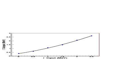
Figure 3: Fitted vaules for $\Gamma_{X(3872)}$ (vertical) versus the MC generator input values (horizontal). The curve is the result of a fit to a second-order polynomial.

A fit to the $X(3872)\rightarrow\pi^{+}\pi^{-}J/\psi$ mass peak in data with $\Gamma_{X(3872)}$ as a free parameter returns a value that is at the lower limit imposed on the fit. To establish an upper limit on its value, we made a study of how the fit likelihood depends on $\Gamma_{X(3872)}$.

In the three-dimensional fit, there are correlations between the fitted width, the numbers of signal events ($n_{\rm sig}$) and peaking background events ($n_{\rm peak}$). The other parameters have negligible correlations with the width. We therefore performed a series of fits to the data where we fixed $\Gamma_{X(3872)}$ at a sequence of values ranging from 0.1 to 3.0 MeV. In these fits all parameters other than $n_{\rm sig}$ and $n_{\rm peak}$ were fixed at their best fit values; $n_{\rm sig}$ and $n_{\rm peak}$ were allowed to vary. Figure 4 shows how the fit likelihood changes with $\Gamma_{X(3872)}$. The arrow in the figure indicates the width value, $\Gamma_{X(3872)}=0.95$ MeV, below which 90% of the integrated area under the points is contained. This value is below the experimental resolution. To check sensitivity to uncertainties in the mass resolution width, we repeated the scan using the value of the tail resolution width determined from fitting the $\psi^{\prime}$ peak without any rescaling. This had negligible effect on the width of the likelihood.

Figure 4: Likelihood values from the $\Gamma_{X(3872)}$ scan described in the text. The region of the plot below the arrow contains 90% of the total area under the points.

In order to evaluate whether our measured limit is reasonable given the size of our data sample, we derived width upper limits from similar analyses of 24 statistically independent, 170-event MC samples that were generated with $\Gamma_{X(3872)}=0$. Of these, twelve produced 90% CL upper limits that are less than 1 MeV; five returned a fit value at the lower limit imposed on the fit. In a set of 24 MC samples generated with $\Gamma_{X(3872)}=1$ MeV, none returned a width value at the lower limit of the fit and 17 produced 90% CL lower limits that exclude zero.

The $\psi^{\prime}$ width has been precisely measured in $e^{+}e^{-}$ BES2 and $p\bar{p}$ E835 threshold scans to be $0.304\pm 0.009$ MeV PDG , a value that is well below the resolution of our measurement. We validated our experimental sensitivity to narrow natural widths by refitting the $\psi^{\prime}$ data sample using resolution parameters fixed at the values given in Table 2 but with $\Gamma_{\psi^{\prime}}$ left as a free parameter. The fit result is $\Gamma_{\psi^{\prime}}=0.53\pm 0.11$ MeV. An examination of the fit likelihood shows that it is well behaved and excludes a zero width value by more than $4\sigma$. The measured value is $0.23\pm 0.11$ MeV above the PDG’s world-average value, which is consistent with the bias value at $\Gamma\simeq 0.3$ MeV derived from the fitted curve in Fig. 3, namely $0.25$ MeV.

As an upper limit on the natural width of the $X(3872)$, we inflate the 90% CL value determined from the scan values shown in Fig. 4 by $0.23$ MeV, the measured difference between our measurement of $\Gamma_{\psi^{\prime}}$ and its world-average value, to account for a possible measurement bias. Since both the simulated and observed biases are positive and indicate that our measured limit is biased high, this produces a conservative value for the upper limit. The result is

$$\Gamma_{X(3872)}<1.2~{}{\rm MeV}~{}~{}~{}~{}~{}{\rm 90\%CL},$$ (5)

which is more restrictive than the previous 90% CL limit of 2.3 MeV skchoi_x3872 .

VI.3 Product branching fractions

We determine product branching fractions for $B^{+}\rightarrow K^{+}X$, $X\rightarrow\pi^{+}\pi^{-}J/\psi$ and $B^{0}\rightarrow K^{0}X$, $X\rightarrow\pi^{+}\pi^{-}J/\psi$ via the relation

$${\mathcal{B}}(B\rightarrow KX(3872))\times{\mathcal{B}}(X(3872)\rightarrow\pi^{+}\pi^{-}J/\psi) =$$

$$\frac{N^{\rm evts}_{K}}{N_{B\bar{B}}\epsilon_{K}f_{K}{\mathcal{B}}_{J/\psi\rightarrow\ell\ell}},$$ (6)

where the notation is the same as that used for Eq. 2. The results are

$${\mathcal{B}}(B^{+}\rightarrow K^{+}X(3872))\times{\mathcal{B}}(X(3872)\rightarrow\pi^{+}\pi^{-}J/\psi) =$$

$$(8.61\pm 0.82~{}{\rm(stat)}\pm 0.52~{}{\rm(syst)})\times 10^{-6},$$ (7)

and

$${\mathcal{B}}(B^{0}\rightarrow K^{0}X(3872))\times{\mathcal{B}}(X(3872)\rightarrow\pi^{+}\pi^{-}J/\psi) =$$

$$(4.3\pm 1.2~{}{\rm(stat)}\pm 0.4~{}{\rm(syst)})\times 10^{-6},$$ (8)

where the systematic error includes uncertainties in the MC simulation of the tracking, particle identification for the leptons and charged kaon, $K_{S}$ reconstruction, uncertainties in the number of $B\bar{B}$ meson pairs, choice of parameterization used in the three dimensional fit, MC statistics, decay model dependence and the error on the world-average $J/\psi\rightarrow\ell^{+}\ell^{-}$ branching fraction, all added in quadrature. The computations are summarized in Table 5. The ratio of the $B^{0}$ and $B^{+}$ product branching fractions is

$$R(X)=\frac{{\mathcal{B}}(B^{0}\rightarrow K^{0}X(3872))}{{\mathcal{B}}(B^{+}\rightarrow K^{+}X(3872))} =$$

$$0.50\pm 0.14~{}{\rm(stat)}\pm 0.04~{}{\rm(syst)},$$ (9)

where the systematic error evaluation is summarized in Table 5. This value is above the range preferred by some molecular models for the $X(3872)$: $0.06\leq R(X)\leq 0.29$ swanson_pr . The BaBar result for this ratio is $R(X)=0.41\pm 0.24\pm 0.05$ babar_pipijpsi .

Table 5: Systematic errors on the product branching fraction measurement.

Source	$K^{+}X(3872)$	$K_{S}X(3872)$	$K_{S}/K^{+}$ Ratio
	(percent)	(percent)	(percent)
$N_{B\bar{B}}$	1.4	1.4	-
Secondary BF	1.0	1.0	-
MC statistics	1.0	1.0	1.4
MC model	2.1	2.1	-
Hadron ID	3.7	2.6	1.1
Lepton ID	1.1	1.1	-
Tracking	1.8	1.4	0.4
3-dim. fit model	3.0	5.0	6.0
$K_{S}$ efficiency	-	4.5	4.5
Quadrature sum	6.0	8.1	7.7

VII Search for a charged partner of the $X(3872)$ in $B\rightarrow K\pi^{+}\pi^{0}J/\psi$ decays

We search for a charged partner of the $X(3872)$ decaying into $\pi^{+}\pi^{0}J/\psi$ using the selection criteria described above for the $\pi^{+}\pi^{-}J/\psi$ analysis, with the exception that one of the charged pions is replaced by a $\pi^{0}$. For this we require two photons with $E_{\gamma}>35$ MeV that reconstruct to a $\pi^{0}\rightarrow\gamma\gamma$ with a mass-constrained fit $\chi^{2}\leq 4.0$. In the event of multiple $\gamma$ entries we choose the candidate with the best $\chi^{2}$ from the $\pi^{0}$ mass-constrained fit; for multiple charged pions, we chose the candidate that produces the lowest value of $|\Delta E|$.

We perform an unbinned two-dimensional ($M_{\rm bc}$ vs. $M(\pi^{+}\pi^{0}J/\psi)$) maximum likelihood fit to the selected event samples using Gaussian and ARGUS function PDFs for the $M_{\rm bc}$ signal and background, and a Crystal Ball function Xtal_ball and third-order polynomial for the $M(\pi^{+}\pi^{0}J/\psi)$ signal and background, respectively. For the peaking background we use the $M_{\rm bc}$ signal PDF and a linear background shape for the $M(\pi^{+}\pi^{0}J/\psi)$ PDF. The Crystal Ball function parameters are fixed at values returned from fits to samples of Monte Carlo simulated $B\rightarrow KX^{+}$, $X^{+}\rightarrow\rho^{+}J/\psi$ events with $m_{X^{+}}=3871.7$ MeV and $\Gamma_{X^{+}}=0$. The results of the fit to the simulated $\bar{B}^{0}\rightarrow K^{-}X^{+}$ sample are shown in the top panels of Fig. 5.

For the data, we do a series of fits with the $X^{+}$ mass restricted to overlapping 10 MeV mass windows covering the range 3850 MeV to 3890 MeV. For the $K^{-}X^{+}$ channel the largest signal yield is $4.2\pm 7.8$ events at a mass of $3873\pm 6$ MeV. The 90% CL upper limit, corresponding to the signal yield below which 90% of the area of the likelihood function is contained, is 17.3 events. For the $K^{0}X^{+}$ channel, all mass intervals have a zero signal yield and the 90% upper limit derived from the likelihood function for a peak mass fixed at $3873$ MeV is 5.4 events. $M_{\rm bc}$ and $M(\pi^{+}\pi^{0}J/\psi)$ plots for the fit to the $K^{-}X^{+}$ sample with the highest event yield are shown in the middle panel of Fig. 5. The bottom panels of Fig. 5 show the results of the fit to the $K^{0}X^{+}$ sample with peak mass fixed at 3873 MeV.

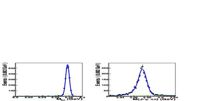
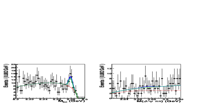
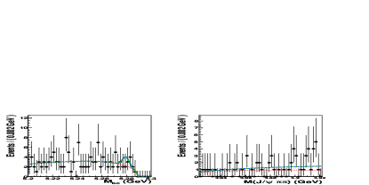
Figure 5: The $M_{\rm bc}$ (left), $M(\pi^{+}\pi^{0}J/\psi)$ (right) distributions for $B\rightarrow KX^{+}(3872)$, $X^{+}\rightarrow\rho^{+}J/\psi$ MC events (top) and $\bar{B}^{0}\rightarrow K^{-}\pi^{+}\pi^{0}J/\psi$ (middle) and $B^{+}\rightarrow K^{0}\pi^{+}\pi^{0}J/\psi$ (bottom) event candidates in the data, within the signal region of the other quantity. The curves show the results of the fits described in the text.

We determine 90% CL product branching fraction upper limits using the relation

$${\mathcal{B}}(B\rightarrow KX^{+})\times{\mathcal{B}}(X^{+}\rightarrow\rho^{+}J/\psi)<\frac{N^{\rm evts}_{\rm 90\%UL}}{N_{B\bar{B}}{\mathcal{B}}_{J/\psi\rightarrow\ell\ell}\epsilon_{K}f_{K}},$$ (10)

where $N^{\rm evts}_{\rm 90\%UL}$ is the upper limit on the event yield for each channel, $f_{K^{+}}=1.0$ and $f_{K^{0}}=0.346$ (as in Eq. 2), and $\epsilon_{K}$ are the MC acceptances reduced by the systematic error: $\epsilon_{K+}=4.5\%$ and $\epsilon_{K^{0}}=2.8\%$. The systematic errors are the same as those listed in Table 5 above, with the additional inclusion of a 3% systematic error associated with data-MC differences in $\pi^{0}$ detection and 2.5% for the increase in the upper bounds when the resolution parameters of the $M(\pi^{+}\pi^{0}J/\psi)$ signal PDF are varied by $\pm 10\%$. The systematic errors are 6% for the $B^{0}\rightarrow K^{-}X^{+}$ and 8% for the $B^{+}\rightarrow K^{0}X^{+}$ channels. The resulting limits are

$${\mathcal{B}}(\bar{B}^{0}\rightarrow K^{-}X^{+})\times{\mathcal{B}}(X^{+}\rightarrow\rho^{+}J/\psi)<4.2\times 10^{-6}$$ (11)

and

$${\mathcal{B}}(B^{+}\rightarrow K^{0}X^{+})\times{\mathcal{B}}(X^{+}\rightarrow\rho^{+}J/\psi)<6.1\times 10^{-6}.$$ (12)

The BaBar limits for the same quantities are ${\mathcal{B}}(\bar{B}^{0}\rightarrow K^{-}X^{+})\times{\mathcal{B}}(X^{+}\rightarrow\rho^{+}J/\psi)<5.4\times 10^{-6}$ and ${\mathcal{B}}(B^{+}\rightarrow K^{0}X^{+})\times{\mathcal{B}}(X^{+}\rightarrow\rho^{+}J/\psi)<22\times 10^{-6}$ babar_pipi0jpsi .

VIII Angular correlation studies

For subsequent analysis, we define a tighter $X(3872)$ signal region that extends $\pm 6$ MeV around the $M(\pi^{+}\pi^{-}J/\psi)$ signal peak. For background estimates we use $\pm 12$ MeV sidebands above and below the signal peak centered at 3852 MeV and 3892 MeV. There are in total 165 events in the signal region; the background content, determined from the scaled sidebands, is $34\pm 3$ events.

Angular distributions for the sequential decays $B\rightarrow KX(3872)$, $X(3872)\rightarrow\rho J/\psi$, $\rho\rightarrow\pi^{+}\pi^{-}$ and $J/\psi\rightarrow\ell^{+}\ell^{-}$ for the $1^{++}$ and $2^{-+}$ cases are given by the LHCb group in Ref. LHCb-PUB-2010-003 . Since both the $B$ and $K$ mesons are scalar particles, an $X(3872)$ meson produced via exclusive $B\rightarrow KX$ decays must have a zero component of angular momentum along its momentum direction in the $B$ rest frame and, thus, its polarization vector, $\vec{\epsilon}_{X}$, must be along this boost direction. This limits the number of independent partial-wave amplitudes needed to describe the decay. Moreover, angular momentum and parity conservation in $X(3872)\rightarrow\rho J/\psi$ decay implies that for $1^{++}$ the $\rho$ and $J/\psi$ are in an $S$- and/or $D$-wave, while for $2^{-+}$ they are in a $P$- and/or $F$-wave. Since the $X(3872)\rightarrow\rho J/\psi$ decay occurs at threshold, only the lower partial wave in each case is considered. With this constraint, the $1^{++}$ has only one decay amplitude: $L=0$ and $S=1$, where $L$ the $\rho$-$J/\psi$ orbital angular momentum and $S$ their spin state. The $2^{-+}$ hypothesis has two independent amplitudes: $L=1$ with $S=1$ or $S=2$, which we denote by $B_{11}$ and $B_{12}$, respectively.

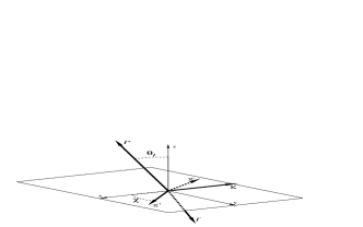
Figure 6: Definitions of the angles $\chi$ and $\theta_{\ell}$ as described in the text.

We denote by $\theta_{X}$ the angle between the $J/\psi$ and the direction opposite to the kaon in the $X(3872)$ restframe. In the case of $J^{PC}=1^{++}$, the $X(3872)\rightarrow\rho J/\psi$ decay produces a $\rho$ and $J/\psi$ in an $S$-wave and, thus, the distribution in $\cos\theta_{X}$ is expected to be flat. For $2^{-+}$, the final state is $P$-wave and the $\cos\theta_{X}$ distribution is $\propto(1+3\cos^{2}\theta_{X})$ for $B_{12}=0$, approximately flat for $|B_{11}|\simeq|B_{12}|$, and $\propto\sin^{2}\theta_{X}$ for $B_{11}=0$. For $1^{++}$ decays to an $S$-wave at threshold, the interaction Lagrangian is ${\mathcal{L}}_{\rm int}\propto\vec{\epsilon}_{X}\cdot(\vec{\epsilon}_{J/\psi}\times\vec{\epsilon}_{\rho})$, where $\vec{\epsilon}_{J/\psi}$ and $\vec{\epsilon}_{\rho}$ polarization vectors. Thus, the three polarization vectors tend to be mutually perpendicular. In polarized $\rho\rightarrow\pi^{+}\pi^{-}$ decays, the pions have a $\cos^{2}\theta$ distribution relative to the $\vec{\epsilon}_{\rho}$ direction, while in polarized $J/\psi\rightarrow\ell^{+}\ell^{-}$, the decay leptons have a $\sin^{2}\theta$ distribution relative to the $\vec{\epsilon}_{J/\psi}$ direction. To exploit this, we use a coordinate system suggested by Rosner rosner where the $x$-axis is the direction opposite to the kaon (i.e., the $\vec{\epsilon}_{X}$ direction), the $x-y$ plane is defined by the kaon and $\pi^{+}$ and the $z$ axis completes a right-handed coordinate system. The angle between the $\pi^{+}$ direction and the $x$-axis is designated as $\chi$ and the angle between the $\ell^{+}$ direction and the $z$-axis as $\theta_{\ell}$, as shown in Fig. 6. In the limit where the $J/\psi$ and $\rho$ are at rest in the $X$ rest frame, the expectation for $1^{++}$ has the distinctive pattern

$$\frac{d^{2}N}{d\cos\theta_{\ell}d\cos\chi}\propto\sin^{2}\theta_{\ell}\sin^{2}\chi.$$ (13)

The changes in the values of $\cos\chi$ and $\cos\theta_{\ell}$ that occur when $\chi$ and $\theta_{\ell}$ are determined in either the $J/\psi$ or $\rho$ restframes (instead of the $X(3872)$ frame) are much smaller than the bin sizes used in this analysis.

The CDF results on angular correlations used a three-dimensional fit to data divided into twelve bins CDF_angles . The limited statistics of our sample preclude dividing the data into enough bins to make a three-dimensional fit feasible. Instead we compare one-dimensional histograms of data and MC for different hypotheses.

The data points in Fig. 7 show the $|\cos\chi|$, $|\cos\theta_{\ell}|$ and $|\cos\theta_{X}|$ distribution for $X(3872)$ signal region events. The dotted histograms indicate the background determined from the events in the scaled $M(\pi^{+}\pi^{-}J/\psi)$ sidebands. The solid histogram is the sum of the background (dotted histogram) and simulated MC $X(3872)\rightarrow\rho J/\psi$ events generated with a $1^{++}$ ($S$-wave only) hypothesis and normalized to the observed signal. (The MC samples described in this section were generated using the partial wave option of EvtGen evtgen .) With no other free parameters, we find good matches between $1^{++}$ expectations and the data for all three distributions: the $\chi^{2}$ values (confidence levels) are $3.82$ (0.43), $1.76$ (0.78) and $0.56$ (0.97) for $|\cos\theta_{X}|$, $|\cos\chi|$ and $|\cos\theta_{\ell}|$, respectively.

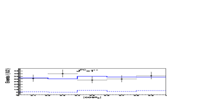
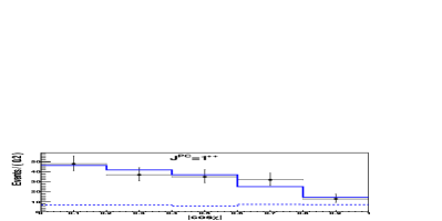
Figure 7: The comparisons described in the text for the $J^{PC}=1^{++}$ hypothesis applied to $|\cos\theta_{X}|$ (top), $|\cos\chi|$ (middle) and $|\cos\theta_{\ell}|$ (bottom). The dashed histograms indicate the sideband-determined background levels.

For $J^{PC}=2^{-+}$, in addition to the normalization, there are two more free parameters that we take to be the ratio $|B_{11}|/|B_{12}|$ and the relative phase between $B_{11}$ and $B_{12}$. A comparison of the measured distributions with those for a MC simulated $2^{-+}$ state with $B_{11}=0$ finds poor matches for all three angular distributions: the $\chi^{2}$ values (confidence levels) are $14.9$ (0.005), $48.8$ ($<10^{-7}$) and $16.5$ (0.002) for $|\cos\theta_{X}|$, $|\cos\chi|$ and $|\cos\theta_{\ell}|$, respectively. For $B_{12}=0$, there are reasonable matches between data and MC for the $|\cos\chi|$ ($\chi^{2}=6.04$, CL=0.20) and $|\cos\theta_{\ell}|$ ($\chi^{2}=1.92$, CL=0.75) distribution, but poor agreement in the case of the $|\cos\theta_{X}|$ comparison ($\chi^{2}=16.2$, CL=0.003).

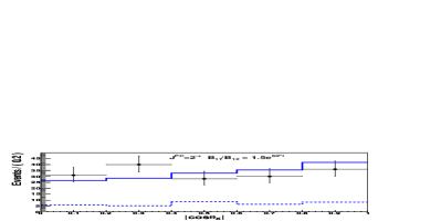
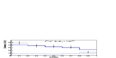
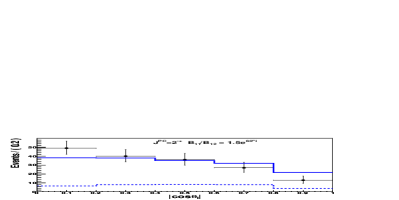
Figure 8: The comparisons described in the text for the $J^{PC}=2^{-+}$ hypothesis applied to $|\cos\theta_{X}|$ (top), $|\cos\chi|$ (middle) and $|\cos\theta_{\ell}|$ (bottom) for $B_{11}/B_{12}=1.5e^{60^{\circ}i}$.

We made similar comparisons with simulated event samples for a grid of values for $|B_{11}|/|B_{12}|$ and its relative phase. Figure 8 shows the data - MC comparison for the case where $(B_{11}/B_{12})=1.5e^{60^{\circ}i}$, the value for which we found the best match. In this case all three MC distributions have acceptable $\chi^{2}$ values (confidence levels): $4.72$ (0.32) for $\cos\theta_{X}$, $4.60$ (0.33) for $\cos\chi$, and $5.24$ (0.26) for $\cos\theta_{\ell}$. The LHCb analysis uses the parameter $\alpha=\frac{B_{11}}{B_{11}+B_{12}}$ LHCb-PUB-2010-003 ; the values of $|B_{11}|/|B_{12}|$ and the relative phase that are listed above translate into $\alpha=0.69e^{23^{\circ}i}$.

We conclude that with the current level of statistical precision we cannot distinguish definitively between the $1^{++}$ and $2^{-+}$ assignments. However, while the $2^{-+}$ MC distributions for all three angles are similar to those for $1^{++}$, they differ in detail, suggesting that in future experiments with larger data samples, such as LHCb LHCb-detector , Belle II belle2_exp and SuperB superb , three-dimensional fits based on the angles discussed here will be able to distinguish between the two $J^{PC}$ hypotheses.

IX Fits to the $M(\pi^{+}\pi^{-})$ distribution

For even-parity $C=+1$ states the $\pi^{+}\pi^{-}J/\psi$ final state would be a $\rho$ and $J/\psi$ primarily in a relative $S$-wave, while for $2^{-+}$, the $\rho$ and $J/\psi$ would be in a relative $P$-wave. For the $S$-wave case, the $M(\pi^{+}\pi^{-})$ mass distribution near the upper kinematic limit is modulated by the available phase space, which is proportional to $k^{*}$, the $J/\psi$ momentum in the $X(3872)$ restframe. For a $J/\psi$ and $\rho$ in a $P$-wave, the upper boundary is suppressed by an additional $(k^{*})^{2}$ centrifugal barrier. Thus, the high-mass part of the $\pi^{+}\pi^{-}$ invariant mass distribution provides some $J^{P}$ information.

We extract a background-subtracted $M(\pi^{+}\pi^{-})$ spectrum from a series of two-dimensional ($M_{\rm bc}$ vs. $\Delta E$) likelihood fits to data in 20 MeV-wide $M(\pi^{+}\pi^{-})$ bins covering the range $0.4~{}{\rm GeV}\leq M(\pi^{+}\pi^{-})\leq 0.78$ GeV. The extracted yields are corrected for the $M(\pi^{+}\pi^{-})$-dependence of the experimental acceptance using results from simulated data samples of $B\rightarrow KX$, $X\rightarrow\rho J/\psi$ events where the $\rho$ mass is artificially set at various masses with a narrow width. The peaking background remaining in the data is estimated from the $M(\pi^{+}\pi^{-}J/\psi)$ sidebands to be $12\pm 5$ events with an $M(\pi^{+}\pi^{-})$ distribution that is similar to that of the $X(3872)$ signal. The resulting distribution is shown as data points with error bars in Fig. 9

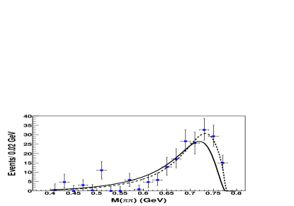
Figure 9: The data points show the background-subtracted, relative-efficiency-corrected $M(\pi^{+}\pi^{-})$ distribution for $X(3872)\rightarrow\pi^{+}\pi^{-}J/\psi$ events. The curves show the results of fits using an $S$-Wave (dashed) and a $P$-Wave (solid) BW function as described in the text.

We fit the $M(\pi^{+}\pi^{-})$ distribution for events in the $X(3872)$ signal region using the parameterization of Ref. cdf_pipi

$$dN/dm_{\pi\pi}\propto(k^{*})^{2\ell+1}f^{2}_{\ell X}(k^{*})|BW_{\rho}(m_{\pi\pi})|^{2},$$ (14)

where $k^{*}$ is defined above, $\ell$ is the orbital angular momentum value, $f_{0X}=1.0$ and $f_{1X}(k^{*})=(1+R_{X}^{2}k^{*2})^{-1/2}$ are Blatt-Weisskopf “barrier factors” bw and $BW_{\rho}$ is the relativistic BW expression

$$BW_{\rho}(m_{\pi\pi})\propto\frac{\sqrt{m_{\pi\pi}\Gamma_{\rho}}}{m^{2}_{\rho}-m^{2}_{\pi\pi}-im_{\rho}\Gamma_{\rho}}.$$ (15)

Here $\Gamma_{\rho}=\Gamma_{0}[q^{*}/q_{0}]^{3}[m_{\rho}/m_{\pi\pi}][f_{1\rho}(q^{*})/f_{1\rho}(q_{0})]^{2}$, where $q^{*}(m_{\pi\pi})$ is the pion momentum in the $\rho$ rest frame, $q_{0}=q^{*}(m_{\rho})$, $f_{1\rho}(q))=(1+R^{2}_{\rho}q^{2})^{-1/2}$, $\Gamma_{0}=146.2$ MeV and $m_{\rho}=775.5$ MeV PDG . The “radii” $R_{X}$ and $R_{\rho}$ are poorly known. Generally $R_{\rho}=1.5$ GeV^-1 is used and CDF uses values for $R_{X}$ that are as large as $R_{X}=5.0$ GeV^-1. (Higher values of $R_{X}$ reduce the effects of the $k^{*(2\ell+1)}$ factor and, therefore, make the $S$- and $P$-wave differences smaller.) We take these values as our default settings.

The smooth curves in Fig. 9 show the results of the $S$-wave (dashed line) and $P$-wave (solid line) fits. The $S$-wave ($\ell=0$) case fits the data well: $\chi^{2}/d.o.f.=17.5/18$ (CL=49%). The $P$-wave ($\ell=1$) fit is poorer, $\chi^{2}/d.o.f.=32.1/18$ (CL=2%). Reducing the Blatt-Weisskopf radius for the $X(3872)$ makes the $P$-wave fit worse, increasing $R_{X}$ to $7.0$ GeV^-1 improves the $P$-wave fit $\chi^{2}/d.o.f.$ to $26.5/18$, which corresponds to a 9.0% CL. Large changes in $R_{\rho}$ are found to have little effect on the fit quality for either case.

However, both Belle belle_3pijpsi and BaBar babar_3pijpsi have reported evidence for the sub-threshold decay process $X(3872)\rightarrow\omega J/\psi$. The CDF group pointed out that interference between the $\rho J/\psi$ and $\omega J/\psi$ final states, where $\omega\rightarrow\pi^{+}\pi^{-}$, can have important effect on the $M(\pi^{+}\pi^{-})$ lineshape near the upper kinematic limit cdf_pipi . We therefore repeated the above-described fits with the inclusion of possible effects from $\rho$-$\omega$ interference.

For these fits we use the form given in Eq. 14 with $BW_{\rho}(m_{\pi\pi})$ replaced by

$$BW_{\rho-\omega}\propto BW_{\rho}+r_{\omega}e^{i\phi_{\omega}}BW_{\omega},$$ (16)

where $BW_{\omega}$ is the same form as $BW_{\rho}$ with $\omega$ meson mass and width values substituted for those of the $\rho$, $r_{\omega}$ is the strength of the $\omega$ amplitude relative to that of the $\rho$, and $\phi_{\omega}$ is their relative phase, which is expected to be $95^{\circ}$ rw_phase .

We performed fits to the $M(\pi^{+}\pi^{-})$ distribution using this form weighted by the acceptance with $\phi_{\omega}$ fixed at $95^{\circ}$ and $r_{\omega}$ left as a free parameter. Figure 10 shows the results of the $S$-wave (dashed line) and $P$-wave (solid line) fits. The inclusion of a small $\omega$ amplitude ($r_{\omega}=0.07\pm 0.05$) improves the $S$-wave fit to $\chi^{2}/d.o.f.=15.8/17$ (54% CL). The $P$-wave fit returns a larger $\omega$ contribution, $r_{\omega}=0.48^{+0.20}_{-0.14}$, and a good fit quality: $\chi^{2}=14.6$ for 17 degrees of freedom ($d.o.f.$) (62% CL).

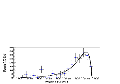
Figure 10: The background-subtracted, relative-efficiency-corrected $M(\pi^{+}\pi^{-})$ distribution for $X(3872)\rightarrow\pi^{+}\pi^{-}J/\psi$ events. The curves show the results of fits using an $S$-Wave (dashed line) and a $P$-Wave (solid line) BW function with effects of $\rho$-$\omega$ interference included.

The fits have three components: direct $\rho\rightarrow\pi^{+}\pi^{-}$ ($\propto|BW_{\rho}|^{2}$) and $\omega\rightarrow\pi^{+}\pi^{-}$ ($\propto r^{2}_{\omega}|BW_{\omega}|^{2}$) contributions and a $\rho$-$\omega$ interference term. The contributions from each component for each fit are listed in Table 6.

Table 6: Summary of the results from the $\rho$-$\omega$ interference fit.

	$N_{sig}$	$r_{\omega}$	$N_{\rho\rightarrow\pi\pi}$	$N_{\omega\rightarrow\pi\pi}$	$N_{\rho-\omega~{}{\rm interf}}$
$S$-wave	$159\pm 15$	$0.07\pm 0.05$	140.9	$0.6\pm 0.5$	17.8
$P$-wave	$158\pm 15$	$0.48^{+0.20}_{-0.14}$	93.2	$3.6^{+1.5}_{-1.1}$	60.0

If the low-mass tails of the $\omega\rightarrow\pi^{+}\pi^{-}\pi^{0}$ and $\omega\rightarrow\pi^{+}\pi^{-}$ lineshapes are the same pko , we expect

$$\frac{N(\omega\rightarrow\pi\pi)}{N_{\rm sig}}=\frac{{\mathcal{B}}(X(3872)\rightarrow\omega J/\psi)}{{\mathcal{B}}(X(3872)\rightarrow\pi^{+}\pi^{-}J/\psi)}\times{\mathcal{B}}(\omega\rightarrow\pi^{+}\pi^{-}),$$ (17)

where the combined result from Belle belle_3pijpsi and BaBar babar_3pijpsi (measured using $\omega\rightarrow\pi^{+}\pi^{-}\pi^{0}$ decays) is ${\mathcal{B}}(X(3872)\rightarrow\omega J/\psi)/{\mathcal{B}}(X(3872)\rightarrow\pi^{+}\pi^{-}J/\psi)=0.8\pm 0.3$. Using this, $N_{\rm sig}=159\pm 15$ and ${\mathcal{B}}(\omega\rightarrow\pi^{+}\pi^{-})=0.0153\pm 0.0013$ PDG , we find an expected value $N(\omega\rightarrow\pi^{+}\pi^{-})=2.0\pm 0.8$ events, which is between the values derived from both the $S$-wave and $P$-wave fits and reasonably consistent with either case.

X Summary

We report a measurement of the difference in masses of $X(3872)$ mesons produced in $B^{+}\rightarrow K^{+}\pi^{+}\pi^{-}J/\psi$ and $B^{0}\rightarrow K^{0}\pi^{+}\pi^{-}J/\psi$ decays,

$$\Delta M_{X(3872)}=(-0.69\pm 0.97~{}{\rm(stat)}\pm 0.19~{}{\rm(syst)})~{}{\rm MeV},$$ (18)

that is consistent with zero and disagrees with theoretical predictions based on a diquark-diantiquark model for the $X(3872)$ maiani . We conclude from this that the same particle is produced in the two processes and use a fit to the combined neutral and charged $B$ meson data samples to determine:

$$M_{X(3872)}=(3871.84\pm 0.27~{}{\rm(stat)}\pm 0.19~{}{\rm(syst)})~{}{\rm MeV}.$$ (19)

This result agrees with the current PDG world-average value of $3871.56\pm 0.22$ MeV PDG and supersedes Belle’s earlier mass measurement skchoi_x3872 , which was based on a 140 fb^-1 subset of the current data sample. The width of the $X(3872)$ signal peak is consistent with the experimental mass resolution and we set a 90% CL limit on its natural width of $\Gamma_{X(3872)}<1.2$ MeV, improving on the previous limit of 2.3 MeV.

We report a new measurement of the product branching fraction

$${\mathcal{B}}(B^{+}\rightarrow K^{+}X(3872))\times{\mathcal{B}}(X(3872)\rightarrow\pi^{+}\pi^{-}J/\psi) =$$

$$(8.61\pm 0.82~{}{\rm(stat)}\pm 0.52~{}{\rm(syst)})\times 10^{-6},$$ (20)

which supersedes the previous Belle result skchoi_x3872 . The $21.0\pm 5.7$ signal event yield for $B^{0}\rightarrow K^{0}X(3872)$ translates to a ratio of branching fractions

$$\frac{{\mathcal{B}}(B^{0}\rightarrow K^{0}X(3872))}{{\mathcal{B}}(B^{+}\rightarrow K^{+}X(3872))}=0.50\pm 0.14~{}{\rm(stat)}\pm 0.04~{}{\rm(syst)}.$$ (21)

An examination of the isospin-related $B\rightarrow K\pi^{+}\pi^{0}J/\psi$ channel shows no evidence for a charged partner to the $X(3872)$ decaying as $X^{+}\rightarrow\rho^{+}J/\psi$ and we determine 90% CL upper limits on the product branching fractions ${\mathcal{B}}(B\rightarrow KX^{+})\times{\mathcal{B}}(X^{+}\rightarrow\rho^{+}J/\psi)$ of $4.2\times 10^{-6}$ and $6.1\times 10^{-6}$ for $K=K^{+}$ and $K=K^{0}$, respectively, for an $X^{+}$ partner state with mass between 3850 MeV and 3890 MeV. These limits are well below expectations for the $X(3872)$ if it is purely a neutral member of an $I=1$ triplet, in which case decays to the $I_{3}=\pm 1$ partners are favored by a factor of two.

A comparison of angular correlations among the final state decay products finds a good match between data and MC expectations for $J^{PC}=1^{++}$ with no free parameters (other than the overall normalization). The $J^{PC}=2^{-+}$ hypothesis has one complex free parameter and we found a value for which this hypothesis also matches the data reasonably well. For this parameter value, the differences between $1^{++}$ and $2^{-+}$ expectations are small but non-zero and a three-dimensional analysis based on the angles that we use could distinguish between the two cases with the much larger data sets expected at the LHCb LHCb-PUB-2010-003 , Belle II belle2_exp and SuperB superb experiments.

Fits to the $M(\pi^{+}\pi^{-})$ mass distribution that only consider contributions from $\rho\rightarrow\pi^{+}\pi^{-}$ decays favor $S$-wave ($J^{P}=1^{+}$) over $P$-wave ($J^{P}=2^{-}$). However, the addition of an interfering contribution from isospin-violating $\omega\rightarrow\pi^{+}\pi^{-}$ decays results in acceptable fits for both the $S$-wave and the $P$-wave hypotheses. The $P$-wave fit requires a more substantial contribution from $\omega\rightarrow\pi^{+}\pi^{-}$, but with the current limited statistics for $X(3872)\rightarrow\pi^{+}\pi^{-}J/\psi$ decays and the poor precision on the ratio ${\mathcal{B}}(X(3872)\rightarrow\omega J/\psi)/{\mathcal{B}}(X(3872)\rightarrow\pi^{+}\pi^{-}J/\psi)$, the measured $\omega\rightarrow\pi^{+}\pi^{-}$ amplitudes that result from fits to $M(\pi^{+}\pi^{-})$ cannot be used to distinguish between the two possibilities. This also may be possible in future experiments.

XI Acknowledgments

We thank the KEKB group for the excellent operation of the accelerator, the KEK cryogenics group for the efficient operation of the solenoid, and the KEK computer group and the National Institute of Informatics for valuable computing and SINET4 network support. We acknowledge support from the Ministry of Education, Culture, Sports, Science, and Technology (MEXT) of Japan, the Japan Society for the Promotion of Science (JSPS), and the Tau-Lepton Physics Research Center of Nagoya University; the Australian Research Council and the Australian Department of Industry, Innovation, Science and Research; the National Natural Science Foundation of China under contract No. 10575109, 10775142, 10875115 and 10825524; the Ministry of Education, Youth and Sports of the Czech Republic under contract No. LA10033 and MSM0021620859; the Department of Science and Technology of India; the BK21 and WCU program of the Ministry Education Science and Technology, National Research Foundation of Korea, and NSDC of the Korea Institute of Science and Technology Information; the Polish Ministry of Science and Higher Education; the Ministry of Education and Science of the Russian Federation and the Russian Federal Agency for Atomic Energy; the Slovenian Research Agency; the Swiss National Science Foundation; the National Science Council and the Ministry of Education of Taiwan; and the U.S. Department of Energy. This work is supported by a Grant-in-Aid from MEXT for Science Research in a Priority Area (“New Development of Flavor Physics”), and from JSPS for Creative Scientific Research (“Evolution of Tau-lepton Physics”). S.-K. Choi acknowledges support from NRF Grant No. KRF-2008-313-C00177 and S.L. Olsen acknowledges support from WCU Grant No. R32-10155.

References

(1)
S.K. Choi et al. (Belle Collaboration),
Phys. Rev. Lett. 91, 262001 (2003).
(2) The inclusion of charge-conjugate modes
is always implied.
(3)
A. Acosta et al. (CDF Collaboration),
Phys. Rev. Lett. 93, 072001 (2004).
(4)
V.M. Abazov et al. (D0 Collaboration),
Phys. Rev. Lett. 93, 162001 (2004).
(5)
B. Aubert et al. (BaBar Collaboration),
Phys. Rev. D 71, 071103 (2005).
(6) N. Brambilla et al.,
Eur. Phys. J. C 71, 1534 (2011).
(7) K. Nakamura et al. (Particle Data Group),
J. Phys. G 37, 075021 (2010).
(8)See, for example,
M.B. Voloshin and L.B. Okun,
JETP Lett. 23, 333 (1976);
M. Bander, G.L. Shaw and P. Thomas,
Phys. Rev. Lett. 36, 695 (1977);
A. De Rujula, H. Georgi and S.L. Glashow,
Phys. Rev. Lett. 38, 317 (1977);
A.V. Manohar and M.B. Wise, Nucl. Phys. B 339, 17 (1993);
N.A. Törnqvist, hep-ph/0308277 (2003);
F.E. Close and P.R. Page, Phys. Lett. B 578, 119 (2003);
C.-Y. Wong, Phys. Rev. C 69, 055202 (2004);
S. Pakvasa and M. Suzuki, Phys. Lett. B 579, 67 (2004);
E. Braaten and M. Kusunoki, Phys. Rev. D 69, 114012 (2004);
E.S. Swanson, Phys. Lett. B 588, 189 (2004);
D. Gamermann and E. Oset, Phys. Rev. D 80, 014003 (2009)
& Phys. Rev. D 81, 014029 (2010).
(9) N.A. Törnqvist, Z. Phys. C 61, 525 (1994).
(10)
See P. Artoisenet, E. Braaten and D. Kang,
Phys. Rev. D 81, 014013 (2010),
C. Hanhart, Yu.S. Kalashnikova and A.V. Nefediev,
Phys. Rev. D 81, 004028 (2007) &
O. Zhang, C. Meng and H.Q. Zheng,
Phys. Lett. B 680, 453 (2009),
and references cited therein.
(11)
K. Abe et al. (Belle Collaboration),
arXiv:hep-ex/0505038.
(12)
A. Abulencia et al. (CDF Collaboration),
Phys. Rev. Lett. 96, 102002 (2006).
(13) V. Bhardwaj et al. (Belle Collaboration),
arXiv:1105.0177[hep-ex], submitted to Physical Review Letters.
(14)
B. Aubert et al. (BaBar Collaboration),
Phys. Rev. Lett. 102, 132001 (2009).
(15)
A. Abulencia et al. (CDF Collaboration),
Phys. Rev. Lett. 98, 132002 (2007).
(16) Joachim Heuser,
Measurement of the Mass and Quantum Numbers of
the X(3872) State. PhD Thesis, University of Karlsruhe,
Karlsruhe, Germany (2008).
(17) Y. Jia, W.-L. Sang and J. Xu, arXiv:1007.4541[hep-ph].
(18)
P. del Amo Sanchez et al. (BaBar Collaboration),
Phys. Rev. D82, 011101 (2010).
(19)
L. Maiani et al., Phys. Rev. D 71, 014028 (2005).
See also M. Karliner and H.J. Lipkin, arXiv:1008.0203[hep-ph].
(20)
B. Aubert et al. (BaBar Collaboration),
Phys. Rev. D 77, 111101(R) (2008).
(21)
A. Abulencia et al. (CDF Collaboration),
Phys. Rev. Lett. 103, 152001 (2009).
(22) E. Braaten, private communication.
This expectation holds for the case where the
is a pure meson. However, the close proximity
of the threshold may induce large
isospin violations, as pointed out by
N.A. Törnqvist, Phys. Lett. B 590, 209 (2004)
and others.
(23)
B. Aubert et al. (BaBar Collaboration),
Phys. Rev. D71, 031501 (2005).
(24) This is all of the data
that was accumulated by the Belle experiment.
(25)
S. Kurokawa and E. Kikutani, Nucl. Instr. and Meth. A 499, 1 (2003),
and other papers included in this volume.
(26)
A. Abashian et al. (Belle Collaboration),
Nucl. Instr. and Meth. A 479, 117 (2002) and
Y. Ushiroda (Belle SVD2 Group),
Nucl. Instr. and Meth. A 511, 6 (2003).
(27) S.-K. Choi et al. (Belle Collaboration),
Phys. Rev. Lett. 94, 182002 (2005).
(28)
F. Fang et al. (Belle Collaboration),
Phys. Rev. Lett. 90, 071801 (2003).
(29) G.C. Fox and S. Wolfram,
Phys. Rev. Lett. 41, 1581 (1978).
(30) Here is used to designate the
charmonium resonance. This is sometimes referred to as .
(31) The detector response is simulated with GEANT 3,
R. Brun et al., GEANT 3.21, CERN Report DD/EE/84-1 (1984).
(32) We use the Evtgen event generator,
D.J. Lange, Nucl. Instr. and Meth. A 462, 152 (2001).
(33) H. Albrecht et al. (ARGUS Collaboration),
Phys. Lett. B 241, 278 (1990).
(34)
H. Guler et al. (Belle Collaboration),
Phys. Rev. D 83, 032005 (2011)
and K. Abe et al. (Belle Collaboration),
Phys. Rev. Lett. 87, 161601 (2001).
(35) This is the probability that a decays as a
(0.5) times the world-average branching fraction
PDG .
(36)
The fit is restricted to the range MeV in
order to avoid the singularity in the BW function at zero.
(37) M. Ablikim et al. (BES2 Collaboration),
Phys. Rev. Lett. 97, 121801 (2006).
(38) M. Andreotti et al. (E835 Collaboration),
Phys. Lett. B 654, 74 (2007).
(39) E.S. Swanson,
Phys. Rep. 429, 243 (2006).
(40) T. Skwarnicki, PhD Thesis, Institute for
Nuclear Physics, Krakow 1986;
DESY Internal Report, DESY F31-86-02 (1986).
(41) N. Mangiafave, J. Dickens and V. Gibson,
LHCb-PUB-2010-003 PHYS (2010).