Comparative study of many-body perturbation theory and time-dependent density functional theory in the out-of-equilibrium Anderson model

Abstract

We study time-dependent electron transport through an Anderson model. The electronic interactions on the impurity site are included via the self-energy approximations at Hartree-Fock (HF), second Born (2B), GW, and T-Matrix level as well as within a time-dependent density functional (TDDFT) scheme based on the adiabatic Bethe-Ansatz local density approximation (ABALDA) for the exchange correlation potential. The Anderson model is driven out of equilibrium by applying a bias to the leads and its nonequilibrium dynamics is determined by real-time propagation. The time-dependent currents and densities are compared to benchmark results obtained with the time-dependent density matrix renormalization group (tDMRG) method. Many-body perturbation theory beyond HF gives results in close agreement with tDMRG especially within the 2B approximation. We find that the TDDFT approach with the ABALDA approximation produces accurate results for the densities on the impurity site but overestimates the currents. This problem is found to have its origin in an overestimation of the lead densities which indicates that the exchange correlation potential must attain nonzero values in the leads.

I Introduction

The process of electron transport through molecules and nanostructures is part of a rapidly growing research area in condensed matter physics Datta_book ; DiVentra_book . On a fundamental level one has to deal with time-dependent processes in an open system where different scattering mechanisms such as electron-electron or electron-phonon interactions are of great importance. These factors make the transport problem not only difficult, but also very rich in physical phenomena. Most of the recent studies in molecular electronics have focused on the description of steady-state transport while neglecting short-time dynamics such as transients and fast switching processes. However, these processes will become increasingly important since fast switching rates play a pivotal role in the operation of future devices.

For the description of electron transport several numerical approaches have been developed that can deal with fully time-dependent systems Gurviz:96 ; StefanucciAlmbladh:04 ; Moldoveanu:07 ; Bokes:08 ; Ryndyk:08 ; MyohanenStanStefanucciLeeuwen:09 ; Andergassen:10 ; Zheng:10 ; Zheng:07 ; FriesenVerdozziAlmbladh:09 ; FriesenVerdozziAlmbladh-2 ; Brandschaedel:10 ; KurthStefanucciAlmbladhRubioGross:05 . Among these are the time-dependent density matrix renormalization group (tDMRG) approach Boulat:08 , time-dependent density functional theory (TDDFT) StefanucciAlmbladh:04 ; KurthStefanucciAlmbladhRubioGross:05 , and self-consistent many-body perturbation theory (MBPT) based on the Kadanoff-Baym (KB) equations MyohanenStanStefanucciLeeuwen:08 ; FriesenVerdozziAlmbladh:09 ; FriesenVerdozziAlmbladh-2 . Each of these methods has its own advantages and disadvantages. To the best of our knowledge, a comparative study of these three approaches on an identical time-dependent system has not been carried out. Such a study would be very valuable for gaining insight into these methods and into the direction in which each method needs to be improved. In the steady-state regime of quantum transport such comparisons of many-body and benchmark approaches were made by Wang et al. WangSpataruHybertsenMillis:08 within the GW-approximation and by Schmitt and Anders SchmittAnders:10 at second Born (2B) and GW level. In both cases good agreement with benchmark results was found in certain parameter ranges. We want to extend these comparisons to the transient regime as well.

Let us give a brief description of the approaches that we use in this work. The tDMRG method is a numerical algorithm based on truncation of the Hilbert space of low-dimensional systems schollwock:04 ; KarraschSchoeller:10 ; KarraschMeden:10 ; MetzerSchoenhammer:11 . In this work we did not carry out such calculations ourselves but we use published tDMRG resultsHeidrichMeisnerFeiguinDagotto:09 as a benchmark for both the TDDFT and MBPT approaches.

In the TDDFT approach Gross_book ; TDDFT_book a system of interacting electrons is mapped, in an exact manner, onto a system of noninteracting electrons moving in an effective time-dependent external potential known as the Kohn-Sham (KS) potential. The KS potential is functionally dependent on the electron density such that it produces a KS wave function with a density identical to the time-dependent density of the interacting system. It is important to note that TDDFT yields in principle the exact time-dependent current through a molecular junction StefanucciAlmbladh:04 ; DiventraTodorov:04 . The use of one-particle equations in TDDFT allows for large scale first-principle calculations on realistic systems. In practice, however, approximations are unavoidable and the accuracy of a TDDFT calculation crucially depends on the quality of the approximate exchange-correlation (XC) potential used. Most applications of TDDFT to quantum transport processesEversWeigendKoentopp:04 ; BaerSeidemanIlaniNeuhauser:04 ; StefanucciAlmbladh:04 ; StefanucciAlmbladh:04-2 ; KurthStefanucciAlmbladhRubioGross:05 ; BurkeCarGebauer:05 ; Saietal:07 use the adiabatic approximation which assumes that the XC-potential instantaneously follows the density profile. This is a reasonable assumption when the density changes are slow on a time-scale of typical lead-to-molecule tunneling rates, and also when the switch-on times of the applied biases are small enough. However, it has also been pointed out that non-adiabatic effects can have substantial influence Saietal:05 ; VignaleDiventra:09 on calculated properties. In such cases there is also a need to introduce spatial non-locality in the density functional because the non-localities in space and time are strongly related by conservation laws VignaleKohn:96 . This relation is virtually unexplored within a quantum transport context. Gaining further insight into this issue is one of the goals of this work.

The MBPT approach based on the KB equationsKadanoffBaym:62 ; Danielewicz:84 has been successfully applied to time-dependent quantum transport for model systemsMyohanenStanStefanucciLeeuwen:08 ; MyohanenStanStefanucciLeeuwen:09 ; FriesenVerdozziAlmbladh:09 ; FriesenVerdozziAlmbladh-2 . The method offers the possibility of including relevant physical processes by means of selection of Feynman diagrams for the self-energy. The electron-electron correlations are thus considered via the many-body self-energy term which is treated perturbatively to infinite order by summation of infinite classes of diagrams. Furthermore by using conserving approximationsBaymKadanoff:61 ; Baym:62 such as the Hartree-Fock (HF), second Born (2B), GW, and T-Matrix approximations we can guarantee that conservation laws are obeyed, which has shown to be very important in quantum transportThygesenRubio:08 ; Strange:11 . In this approach one has direct access to quantities like quasiparticle spectra, lifetimes, and screened interactions which provide insight into the effects of electron correlation. In particular, the non-locality in time of the 2B, GW, and T-Matrix approximations allows for a description of memory effects and quasi-particle broadening. We use the partition-free scheme where the device is initially contacted to the leads and the whole system in thermal equilibrium Cini:80 . In this approach both the transient and steady-state currents have a direct physical meaning as these currents are induced by the physical switch-on of a bias. In the partitioned approaches they are instead induced by switch-on of a device-lead coupling which does not correspond to the standard experimental situation. We finally like to point out that the MBPT approach can be used to derive new improved time-dependent density functionals with memory and conserving properties vonBarthetal2005 . This has been done successfully within the linear response regime Hellgren ; Hellgren:10 .

Since both TDDFT and MBPT require the use of approximations it is important to have independent benchmark results. For the Anderson impurity model such results in the time domain have recently been obtained with tDMRG HeidrichMeisnerFeiguinDagotto:09 . Therefore we will use this system as a test case for our comparative study of MBPT and TDDFT. The paper is organized as follows: in Sec. II we introduce the model used in our investigation. In Sections II.1 and II.2 we describe the MBPT and the TDDFT methods used. In Sec. III we present numerical results and the last section summarizes our conclusions.

II The model

We study an Anderson impurity modelAnderson:61 described by the Hamiltonian

$$\hat{H}(t)=\hat{H}_{\textrm{\tiny C}}+\sum_{\alpha}\hat{H}_{\alpha}(t)+\hat{H}_{\rm{\tiny T}},$$ (1)

where $\hat{H}_{\rm{\tiny C}}$, $\hat{H}_{\alpha}$, and $\hat{H}_{\textrm{\tiny T}}$ respectively describe the impurity region, the leads $\alpha$ (= L,R), and the tunneling between the impurity region and the leads. The Hamiltonian for the impurity site reads

$$\hat{H}_{\textrm{\tiny C}}=\sum_{\sigma}\varepsilon_{0}\hat{c}_{0\sigma}^{\dagger}\hat{c}_{0\sigma}+\frac{1}{2}\sum_{\sigma,\sigma^{\prime}}U\hat{c}_{0\sigma}^{\dagger}\hat{c}_{0\sigma^{\prime}}^{\dagger}\hat{c}_{0\sigma^{\prime}}\hat{c}_{0\sigma},$$ (2)

where $c_{\sigma}^{\dagger},c_{\sigma}$ are fermionic creation and annihilation operators and ${\sigma,\sigma^{\prime}}$ are the spin indices, $\varepsilon_{0}$ is the on-site energy of the interacting site and $U$ is the interaction term or the charging energy. The Hamiltonian $\hat{H}_{\alpha}(t)$, describing the leads is

$$\hat{H}_{\alpha}(t) = \sum_{\begin{subarray}{c}\sigma\end{subarray}}\sum_{\begin{subarray}{c}i=1\end{subarray}}^{\infty}\Big{(}\varepsilon_{\alpha}+W_{\alpha}(t)\Big{)}\hat{c}_{i\sigma\alpha}^{\dagger}\hat{c}_{i\sigma\alpha}$$ (3)

$$-\sum_{\begin{subarray}{c}\sigma\end{subarray}}\sum_{\begin{subarray}{c}i=1\end{subarray}}^{\infty}\Big{(}V_{\alpha}\hat{c}_{i\sigma\alpha}^{\dagger}\hat{c}_{i+1\sigma\alpha}+H.c.\Big{)},$$

where $\varepsilon_{\alpha}$ is the on-site energy in the leads, $W_{\alpha}$ is the bias on the lead $\alpha$ and $V_{\alpha}$ is the hopping between neighboring lead sites. The tunneling Hamiltonian describes the coupling between the impurity site and the leads, and has the form

$$\hat{H}_{\textrm{\tiny T}}=-\sum_{\sigma}\left(V_{\textrm{link}}\,\hat{c}_{0\sigma}^{\dagger}\hat{c}_{1\sigma L}+V_{\textrm{link}}\,\hat{c}_{0\sigma}^{\dagger}\hat{c}_{1\sigma R}+H.c.\right),$$ (4)

where $V_{\textrm{link}}$ is the hopping from the leads to the impurity site and vice versa.

II.1 Kadanoff-Baym equations

The nonequilibrium properties of the system are studied with the aid of nonequilibrium Green function theory and TDDFT described later in section II.2. The nonequilibrium Green function is defined as the expectation value with respect to the initial state of the contour-ordered product of creation and annihilation operators Danielewicz:84

$$G_{i\sigma,j\sigma^{\prime}}(z,z^{\prime}) = -i\big{\langle}\mathcal{T}[\hat{c}_{H,i\sigma}(z)\hat{c}_{H,j\sigma^{\prime}}^{\dagger}(z^{\prime})]\big{\rangle},$$ (5)

where $i,j$ are the site-indices, $\mathcal{T}$ denotes the time-ordering operator along the Keldysh contour Danielewicz:84 , and where the contour variables $z$ and $z^{\prime}$ specify the position on the contour intro_Keldysh:08 . The subscript $H$ refers to operators in the Heisenberg picture with respect to the time-dependent Hamiltonian $\hat{H}(z)$ Danielewicz:84 ; intro_Keldysh:08 . The Green function of the whole system satisfies the equation of motion

$$[i\partial_{z}\mathbf{1} - \mathbf{H}(z)]{\bf G}(z,z^{\prime})=\delta(z,z^{\prime})\mathbf{1}+$$ (6)

$$+ \int_{\mathcal{C}}\textrm{d}\bar{z}\;\mathbf{\Sigma}^{\textrm{\tiny MB}}[{\bf G}](z,\bar{z}){\bf G}(\bar{z},z^{\prime}),$$

where we introduced the many-body self-energy $\Sigma^{\textrm{\tiny MB}}[G]$ which accounts for all the exchange and correlation effects MyohanenStanStefanucciLeeuwen:09 and where we suppressed spatial indices. The self-energy is a functional of the Green function which in practice is defined diagrammatically Danielewicz:84 ; KadanoffBaym:62 .

In this work we solve the equation of motion of the Keldysh Green function fully self-consistently dahlen06procKB ; DahlenLeeuwen:07 ; sdvl.2009method ; sdvl.2009gw using the four approximations of the many-body self-energy $\Sigma^{\textrm{\tiny{MB}}}[G]$ shown in Fig. 1. The self-consistent HF approximation is time-local and includes the Hartree and the exchange potential. The self-consistent 2B approximation consists of the two diagrams to second order in the interaction DahlenLeeuwen:05 . It describes dynamical screening of the electron-electron interaction via a simple bubble diagram and includes a vertex contribution via the second order exchange diagram. The fully self-consistent GW approximation Hedin incorporates the dynamical screening effects via the infinite summation of bubble diagrams sdvl.2009gw . In this approximation, the Coulomb interaction is replaced by the screened potential $W$. The last approximation we use is the fully self-consistent T-matrix approximation KadanoffBaym:62 ; Danielewicz:84 . It contains the 2B diagrams and an infinite summation of the ladder diagrams. The GW and T-matrix approximations are complementary since the GW approximation accounts for dynamical screening in infinite systems with long-range Coulombic interactions whereas the T-matrix approximation is known to be important in describing infinite systems with a short range hard-core interaction KadanoffBaym:62 ; fetter .

When we describe a system attached to noninteracting leads the equation of motion of the Green function for the whole system can be folded into an effective equation of motion of the Green function for the central region MyohanenStanStefanucciLeeuwen:09 ; MyohanenStanStefanucciLeeuwen:08 . In the case of the impurity model that we consider this gives

$$\left[i\partial_{z}-H(z)\right]G(z,z^{\prime})=\delta(z,z^{\prime})$$

$$+\int_{\mathcal{C}}\,\textrm{d}\bar{z}\,\Big{\{}\big{[}\Sigma_{\textrm{em}}(z,\bar{z})+\Sigma^{\textrm{\tiny MB}}[G](z,\bar{z})\big{]}G(\bar{z},z^{\prime})\Big{\}},$$

where the embedding self-energy $\Sigma_{\textrm{em}}(z,z^{\prime})$ accounts for the tunneling of electrons between leads and the impurity site. The many-body self-energy depends only on the Green function of the central site as the many-body interaction is restricted to the central site only. This Green function has only one spatial index.

Figure 1: Diagrammatic representation of the conserving many-body approximations to the self-energy. Wiggly lines denote the many-body interaction. All Green function lines (directed solid lines) are are fully dressed.

For the time-dependent observables calculated on the real axis we denote the contour parameter $z$ by the real time $t$. The time-dependent density for the impurity site is given by

$$n_{0}(t)=-i\,G^{<}(t,t^{+}),$$ (8)

where $t^{+}$ approaches $t$ from an infinitesimally later time $t^{+}=t+\delta$. The current through the lead $\alpha=$ (L,R) can be expressed in terms of the so-called Keldysh Green functions as MyohanenStanStefanucciLeeuwen:09 ; MyohanenStanStefanucciLeeuwen:08

$$\textrm{I}_{\alpha}(t) = 2\textrm{Re}\bigg{\{}\int_{t_{0}}^{t}d\bar{t}[G^{<}(t,\bar{t})\Sigma_{\rm em,\alpha}^{\textrm{\tiny A}}(\bar{t},t)$$ (9)

$$+ \int_{t_{0}}^{t}d\bar{t}G^{\textrm{\tiny R}}(t,\bar{t})\Sigma_{\rm em,\alpha}^{<}(\bar{t},t)]$$

$$-i \int_{0}^{\beta}d\bar{\tau}G^{\rceil}(t,\bar{\tau})\Sigma_{\rm em,\alpha}^{\lceil}(\bar{\tau},t)\bigg{\}},$$

where we integrated on the Keldysh contour and where the superscripts $\rm A,R$ and $\rm<$ refer to the advanced, retarded, and lesser components of the Green function and the self-energy. Further, $\rceil$ and $\lceil$ are the mixed components having one time argument on the imaginary axis and another on the real axis sdvl.2009method ; MyohanenStanStefanucciLeeuwen:09 . The initial many-body correlations and embedding effects are taken into account by the last term in equation (9) which is an integral over the vertical track of the Keldysh contour intro_Keldysh:08 . If we assume that in the $t\to\infty$ limit the terms with components on the imaginary track vanish and that the Green function and the self-energy depend only on $t-t^{\prime}$ then we can Fourier transform (9) and we obtain the Meir-Wingreen formula for the steady-state current MeirWingreen:92

$$I_{\alpha}^{\infty}=-i\int_{-\infty}^{\infty}\frac{d\omega}{\pi}\Gamma_{\alpha}(\omega)\Big{[}G^{<}(\omega)-2i\pi f_{\alpha}(\omega)A(\omega)\Big{]}$$ (10)

where $\Gamma_{\alpha}(\omega)$ is the imaginary part of the embedding self-energy, $f_{\alpha}(\omega)$ is the Fermi function and $A(\omega)$ is the steady-state spectral function MeirWingreen:92 . Hence, equation (9) is a generalization of the Meir-Wingreen formula MyohanenStanStefanucciLeeuwen:09 .
We further define the nonequilibrium spectral function

$$A(T,\omega)=-\textrm{Im}\int\frac{\textrm{d}\tau}{\pi}e^{i\omega\tau}\big{[}G^{>}-G^{<}\big{]}(T+\frac{\tau}{2},T-\frac{\tau}{2}),$$ (11)

where $\tau=t-t^{\prime}$ is a relative time and $T=(t+t^{\prime})/2$ is an average time-coordinate dahlen06procKB2 ; MyohanenStanStefanucciLeeuwen:09 ; uimonen:10 . In equilibrium, this function is independent of $T$ and has peaks below the Fermi level at the electron removal energies of the system, while above the Fermi level it has peaks at the electron addition energies. If the time-dependent external field becomes constant after some switching time, then also the spectral function becomes independent of $T$ after some transient period and has peaks at the addition and removal energies of the biased system MyohanenStanStefanucciLeeuwen:10 .

II.2 Time-dependent density functional theory

Within TDDFT the complication brought forward by considering an open system can be resolved in a very similar manner as in MBPT (see Section II.1), with the aid of an embedding self-energy. The equation of motion for the $k$-th single-particle orbital is projected onto the Anderson impurity site and reads

$$\left[i\partial_{t}-H^{\textrm{\tiny KS}}(t)\right]\psi_{k}(t)=\int_{0}^{t}{\rm d}\bar{t}\;\Sigma_{\rm KS}^{\textrm{\tiny R}}(t,\bar{t})\psi_{k}(\bar{t})$$

$$+\sum_{\alpha}V_{\textrm{link}}\,g_{\alpha\alpha}^{\textrm{\tiny R}}(t,0)\psi_{k,\alpha}(0),$$ (12)

where $\Sigma_{\rm KS}^{\textrm{\tiny R}}(t,\bar{t})$ is the KS embedding self-energy and $g_{\alpha\alpha}^{\textrm{\tiny R}}$ is the retarded lead Green function. This expression is, in principle, exact. If we now assume that the exchange-correlation potential is zero in the leads then $\Sigma_{\rm KS}^{\textrm{\tiny R}}(t,\bar{t})$ can be replaced by $\Sigma_{\rm em}^{\textrm{\tiny R}}(t,\bar{t})$ of Eq.(6). We will assume this in the following. Then for the Anderson impurity model the KS Hamiltonian $H^{\textrm{\tiny KS}}(t)$ has the following from

$$H^{\textrm{\tiny KS}}(t) = v_{\rm KS}(t)$$ (13)

$$= \varepsilon_{0}(t)+\frac{1}{2}Un_{0}(t)+v_{\rm xc}[n](t).$$

The approximation for the XC-potential in this work is based on the local density approximation (LDA) for the static, non-uniform one-dimensional Hubbard model derived from the Bethe ansatz (Bethe ansatz LDA, BALDA) which has been suggested in Ref. [schonhammerGunnarssonNoack:95, ] and further been developed in Ref. [LimaSilvaOliveiraCapelle:03, ]. The adiabatic version Verdozzi:08 of this functional (ABALDA) makes $v_{\rm xc}[n]$ local in both space and time. The modified version of ABALDA for the transport setup KurthStefanucciKhosraviVerdozziGross:10 is taking into account the different hopping between the impurity site and the leads and reads explicitly

$$v^{\textrm{BALDA}}_{\rm xc}[n]=\theta(1-n)v_{\rm xc}^{<}(n)-\theta(n-1)v_{\rm xc}^{<}(2-n),$$ (14)

where

$$v_{\rm xc}^{<}(n)=-\frac{1}{2}Un-2\,V_{\textrm{link}}\left[\cos\left(\frac{\pi n}{2}\right)-\cos\left(\frac{\pi n}{\xi}\right)\right].$$ (15)

Here, $\xi$ is a parameter determined by the equation

$$\frac{2\xi}{\pi}\sin(\pi/\xi)=4\int_{0}^{\infty}{\rm d}x\,\frac{J_{0}(x)J_{1}(x)}{x[1+\exp({U}x/(2\,V_{\textrm{link}}\,))]},$$ (16)

and $J_{i=0,1}(x)$ are Bessel functions. A particularly interesting property of the BALDA is its discontinuity at half-filling LimaOliveiraCapelle:02 : $v_{\rm xc}(1^{+})-v_{\rm xc}(1^{-})=U-4V_{\textrm{link}}\cos(\frac{\pi}{\xi})$. For the parameters used in this work (see Fig. 2), the discontinuity is both positive and negative. However, even if the physical gap should be positive, the results appear not to be affected by this change in sign KurthStefanucciKhosraviVerdozziGross:10 . New parametrizations that alleviate this issue are currently being developed Franca:11 .

The adiabatic approximation implies that

$$\frac{\delta v_{\rm xc}[n](t)}{\delta n(t^{\prime})}=\delta(t-t^{\prime})\,f_{\rm xc}(n(t)),$$ (17)

where $f_{\rm xc}=dv_{\rm xc}(n)/dn$, meaning the XC-response kernel is local in time (and in space). This local and instantaneous approximation becomes valid for Hubbard systems in the limit of slowly varying density both in space and in time. These conditions are not satisfied for the quantum transport system under consideration. Despite this fact, reasonable densities were obtained using the BALDA for finite Hubbard chains Verdozzi:08 and it is therefore worthwhile to try the approximation for quantum transport phenomena. In the present case this approximation for $v_{\rm xc}$ is only used on the impurity interacting site, since no interactions in the leads are present.

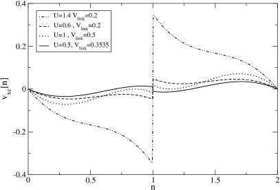
Figure 2: The BALDA XC-potential as a function of the density for parameters used in the subsequent sections.

For future reference we make a connection with the many-body approach of the previous section. The fully self-consistent Green function for the whole system (i.e. leads plus impurity) satisfies the following equation

$$G_{ij}(z,z^{\prime}) = G^{\textrm{\tiny KS}}_{ij}(z,z^{\prime})$$ (18)

$$+ \sum_{kl}\int\!\!{\rm d}\bar{z}d\bar{z}^{\prime}G^{\textrm{\tiny KS}}_{ik}(z,\bar{z})[\Sigma_{kl,{\rm{xc}}}(\bar{z},\bar{z}^{\prime})$$

$$- \delta(\bar{z},\bar{z}^{\prime})\delta_{kl}{v}_{k,\rm xc}(\bar{z})]G_{lj}(\bar{z}^{\prime},z^{\prime}).$$

Since the exact density is given by both the KS and the exact Green function, i.e., $n_{k}(z)=-iG_{kk}(z,z^{+})=-iG_{kk}^{\textrm{\tiny KS}}(z,z^{+})$, it follows that

$$\sum_{k}\int_{\mathcal{C}}\textrm{d}\bar{z}\,G_{ik}^{\textrm{\tiny KS}}(z,\bar{z})v_{k,\rm xc}(\bar{z})G_{ki}(\bar{z},z)=$$

$$\sum_{kl}\int_{\mathcal{C}}\textrm{d}\bar{z}\textrm{d}\bar{z}^{\prime}\,G_{ik}^{\textrm{\tiny KS}}(z,\bar{z})\Sigma_{kl,{\rm{xc}}}(\bar{z},\bar{z}^{\prime})G_{li}(\bar{z}^{\prime},z),$$ (19)

where $\Sigma_{\rm xc}$ is the many-body self-energy with the Hartree potential subtracted. If the self-energy is exact then the corresponding XC-potential that solves this Sham-Schlüter equation rvl:96 yields the exact density of the system. We see that the integral kernel on the left hand side of this equation is nonlocal in space and time. Hence, the solution of this integral equation for $v_{k,{\rm xc}}$ will in general have values on any site $k$. This has been confirmed by recent work of Schenk et al. Schenk:11 . It is important to note that this is true even if the many-body interactions are restricted to the impurity site only. We therefore make an approximation if we set the XC-potential to zero in the leads. We will discuss the validity of this approximation in the results section.

III Transport through a weakly coupled correlated site

We perform many-body and density-functional transport calculations for the Anderson impurity model. The one-site model is fully specified by three parameters: the Hubbard interaction (or charging energy) $U$, the on-site energy $\varepsilon_{0}$ and the hopping $V_{\textrm{link}}$ connecting the interacting impurity site to leads. The leads on-site energies are $\varepsilon_{L}=\varepsilon_{R}=0$ and the hopping in the left and right lead $V_{L}=V_{R}=V$. All parameters are given in units of the lead hopping $V$. For times $t<0$ the contacted system is in equilibrium at zero temperature $(\mu=\varepsilon_{F})$ and Fermi energy $\varepsilon_{F}$. A constant bias $W_{\alpha}$ in lead $\alpha=$ (L,R) is suddenly switched on at $t=0$ after which the time-dependent observables are calculated. We only consider weak coupling to the leads, i.e., $V_{\textrm{link}}\ll V$, since in this regime the role of correlation effects is enhanced. The equilibrium Green function is obtained as the self-consistent solution of the Dyson equation sdvl.2009gw for different approximate many-body self-energies. In the TDDFT calculations the initial state is obtained by a self-consistent static DFT calculation StefanucciAlmbladh:04 . For the XC-potential we use the modified BALDA defined in Section II.2.

III.1 Equilibrium results

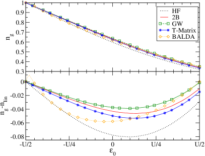
Figure 3: Ground-state density $n_{g}$ on the correlated site versus the on-site energy, $\varepsilon_{0}$, for $U=1$, $V_{\textrm{link}}=0.5$ and $\varepsilon_{F}=0$. In the bottom panel we subtracted $n_{\rm lin}(\varepsilon_{0})=a\varepsilon_{0}+b$ in order to enhance the difference between the curves. The constants $a$ and $b$ are such that $n_{\rm lin}(-U/2)=1$ and $n_{\rm lin}(U/2)=0.35$.

We start by considering a system with interaction $U=1$ and coupling to leads $V_{\textrm{link}}=0.5$. The Fermi energy of the system is $\varepsilon_{F}=0$ (half-filling). In Fig. 3 we display the ground-state density $n_{g}$ on the correlated site for all values of the on-site energy, $\varepsilon_{0}$, for the density functional BALDA and the many-body HF, 2B, GW, and T-Matrix approximations. For $\varepsilon_{0}=-U/2$ the system is invariant under the particle-hole transformation $\hat{d}_{j\sigma}\rightarrow(-)^{j}\hat{d}^{{\dagger}}_{j\sigma}$ and therefore the exact density on the impurity site equals $n_{g}=1$. This remains valid in all the approximation schemes employed. If we increase the gate potential $\varepsilon_{0}$ away from the particle-hole symmetric point, the density on the impurity site decreases almost linearly in all approximations. In order to enhance the differences between the approximations, in the bottom panel we plot $n(\varepsilon_{0})-n_{\rm lin}(\varepsilon_{0})$ where $n_{\rm lin}(\varepsilon_{0})=a\varepsilon_{0}+b$ and the constants $a$ and $b$ are chosen such that $n_{\rm lin}(-U/2)=1$ and $n_{\rm lin}(U/2)=0.35$. In the vicinity of the particle-hole symmetric point, the BALDA has a cusp that is responsible for correlation induced density fluctuations on the impurity site. This gives a time-dependent description of the Coulomb blockade KurthStefanucciKhosraviVerdozziGross:10 . The HF approximation can describe the Coulomb blockade provided we allow the spin symmetry to be broken. The many-body approximations that we use here do not seem to be able to describe the Coulomb blockade without spin-symmetry breaking WangSpataruHybertsenMillis:08 although the onset of the Coulomb blockade is observed SchmittAnders:10 . It can be concluded from the above observations that BALDA yields the Coulomb blockade without spin symmetry breaking KurthStefanucciKhosraviVerdozziGross:10 . For $\varepsilon_{0}<-U/4$ the XC-potential is close to zero and BALDA consequently differs substantially from the correlated MBPT results and follows more closely the HF curve. When $\varepsilon_{0}$ attains positive values, the correlation potential is large and negative, favoring charge accumulation (see Fig. 2). Consequently, the BALDA deviates from HF and follows the correlated MBPT results, in particular with the GW results for $\varepsilon_{0}$ around $U/2$. As a general feature, we find that correlations favor the presence of electrons on the interacting site, since the density in the BALDA and the many-body approaches is larger than the HF density for all values of the on-site energy.

III.2 Nonequilibrium steady-state results

We now shift our attention to the nonequilibrium case. In the left panel of Fig. 4 we display the steady-state density and current (within ABALDA, HF, and 2B) for a symmetrically applied bias $W_{L}=-W_{R}=W/2$ and for three different values of the on-site energy $\varepsilon_{0}=-U/2\,,0\,,U/2$. To improve the clarity of the plot we do not display the results for GW and T-Matrix as they are, in this parameter range, in close agreement to those obtained within 2B. In the left panel of Fig. 4 we see that the 2B, HF, and ABALDA densities are generally in good agreement with each other.

For the corresponding steady-state current, benchmark results are available from tDMRG calculations (see Ref. HeidrichMeisnerFeiguinDagotto:09, ). In the right panel of Fig. 4 we plot the currents as a function of the bias $W/U$. Because the current is proportional to the overlap of the energy bands of the leads, for higher biases, i.e., $W/U>1.5$, the steady-state current decrease with increasing bias.

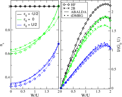
Figure 4: Steady-state density $n_{s}$ (left) and current $I$ (right) for a symmetrically applied bias $W_{L}=-W_{R}=W/2$ and for three different values of the on-site energy $\varepsilon_{0}$. The rest of the parameters are $U=1$, $V_{\textrm{link}}=0.5$ and $\varepsilon_{F}=0$.

We note that for small bias values all the approximations yield values for the current which are on top of the numerically exact tDMRG results for all on-site energies considered. However, for higher biases, only the current obtained within 2B follows closely the tDMRG values for all on-site energies. Therefore, in this range of parameters, we will use the 2B results for benchmarking the other approximations. For $\varepsilon_{0}=U/2$, the HF and ABALDA results follow closely the tDMRG and 2B curves, and for the whole bias-range. For higher biases and smaller on-site energies, i.e. $\varepsilon_{0}=0$ and $\varepsilon_{0}=-U/2$, they considerably overestimate the exact results. However, the conductances, i.e. the initial slopes of the I-V curves in Fig. 4, still remain in close agreement with the 2B approximation and the tDMRG approach. This agrees with the Friedel sum rule that relates the conductance to the density MeraStefanucci:10 .

For the results displayed in Fig. 5 we considered the same system parameters and plotted the density (left panel) and the current (right panel) for an asymmetrically applied bias $W_{L}=W$, $W_{R}=0$. The overlap between the lead energy bands starts to decrease for $W/U>1$ and, consequently, the currents decrease with increasing bias. The steady-state densities behave similarly to the case of symmetric biases (see Fig. 4): the ABALDA and the HF results are in agreement with 2B results except for the case of gate potential $\varepsilon_{0}=0$ at high bias. For the steady-state current (left panel) we also see the same trend: the ABALDA results are close to the HF results and overestimate the 2B results. We observe the same trends as in the case of symmetric bias (see Fig. 4) which indicates that the 2B approximation also here gives a description close to the exact result.

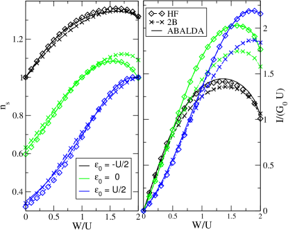
Figure 5: Steady-state density $n_{s}$ (left) and current $I$ (right) for a asymmetrically applied bias $W_{L}=W$, $W_{R}=0$ and for three different values of the on-site energy $\varepsilon_{0}$. The rest of the parameters are $U=1$, $V_{\textrm{link}}=0.5$ and $\varepsilon_{F}=0$.

III.3 Time-dependent results: Adiabatic effects

We now study the performance of the different approximations in the description of transient phenomena. The results are compared to the numerically exact tDMRG data of Ref. HeidrichMeisnerFeiguinDagotto:09, , obtained for a lead-impurity hopping parameter $V_{\textrm{link}}=0.3535$. This decrease in the hopping parameter amounts to a slight enhancement of correlations as compared to the steady-state results of the previous section. The tDMRG calculations HeidrichMeisnerFeiguinDagotto:09 were done for a particle-hole symmetric situation with $\varepsilon_{0}=-U/2$. In addition, we compare the many-body results with ABALDA for the on-site potential $\varepsilon_{0}=U/2$, which is away from the discontinuity of the $v_{\rm xc}$.

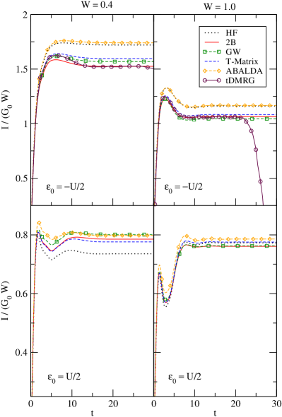
Figure 6: Transient currents for different values of the applied bias $W_{L}=-W_{R}=W/2$, $U=0.5$ and $V_{\textrm{link}}=0.3535$. In the upper panels, $\varepsilon_{0}=-U/2$ corresponds to the particle-hole symmetric point. In the lower panels $\varepsilon_{0}=U/2$.

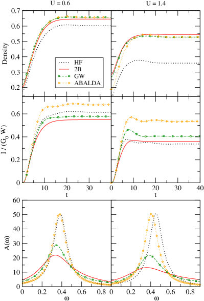
Figure 7: (Color online) Time-dependent density $n_{0}(t)$ for a system with Fermi energy $\varepsilon_{F}=0$, and $\varepsilon_{0}=0.2$, $V_{\textrm{link}}=0.2$ and for different values of the charging energy $U=0.6$ (left column), $1.4$ (right column). The system is driven out of equilibrium by an external bias $W_{L}=0.4$ and $W_{R}=0$. The constant $G_{0}=e^{2}/(2\pi\hbar)=1/(2\pi)$ is the quantum of conduction in atomic units.

In the upper panels of Fig. 6 we display the transient currents as a function of time for the various many-body approaches and the ABALDA as compared to the benchmark tDMRG data. Since the tDMRG calculations are performed on finite systems, one sees the influence of reflections at the system boundaries after a sufficiently long propagation time. The many-body results beyond HF are all in good agreement with the tDMRG results, the most accurate one being the 2B approximation. Not only the values of the steady-state current but also the characteristic bump in the transient is well-reproduced. The ABALDA and the HF approximations perform very similarly; they overestimate the values of the steady-state current and for a bias value of $W=0.4$ they underestimate the height of the transient bump. Also the many-body approximations underestimate the height of the bump somewhat. However, the best agreement is again found for the 2B approximation. It is difficult to pinpoint the origin of the different behavior of the transient bump in the ABALDA and HF when compared to results obtained within correlated approximations. It is worth emphasizing, however, that in time-local approximations such as HF the terms responsible for the initial correlation in the current formula of Eq. (9), i.e., the terms with components on the vertical track of the Keldysh contour, are lacking. In general these terms lead to damping and hence time-local approaches such as HF tend to overshoot the bump in the transient current MyohanenStanStefanucciLeeuwen:09 . In the upper left panel of Fig. 6 such overshoots for the HF and ABALDA are probably masked by the fact that the final steady state current goes to a value that is too large. We finally like to point out that in systems with more levels the transient structure has a more rich oscillatory time-dependence which can be used to analyze the level structure of the central molecule MyohanenStanStefanucciLeeuwen:09 . In these cases the differences between the HF and the correlated approaches become more visible.

In the lower panels of Fig. 6, we display the transient currents the on-site energy on the impurity site being $\varepsilon_{0}=U/2$. The transients show a more pronounced oscillatory behavior because of the increased energy-gap between the impurity level and the Fermi level of the right lead. This determines the oscillation frequency in the transient current (see Ref. MyohanenStanStefanucciLeeuwen:09, ). The many-body approaches agree well with each other whereas the HF approximation underestimates the value of the steady-state current for lower biases. In this case the ABALDA results agree closely with the correlated many-body results. Due to the increased on-site energy $v_{\rm xc}$ becomes negative favoring charge accumulation on the Anderson impurity site (see Fig. 2 and Section III.1).

In order to increase the effects of correlation we now reduce the hopping between the interacting site and leads to $V_{\textrm{link}}=0.2$ and consider two different charging energies $U=0.6$ and $U=1.4$. We also set $\varepsilon_{0}=0.2$ and the Fermi energy to $\varepsilon_{F}=0$. The system is driven out of equilibrium by a sudden switch-on of a constant, asymmetric bias $W_{L}=0.4$, $W_{R}=0$.

In the upper row of Fig. 7 we show the time-dependent density for the interacting site. For $U=0.6$, all results obtained within correlated approximations are in close agreement to each other since if the interaction approaches zero, all MBPT approximations become homologous. As discussed before, in this regime ABALDA and HF are close to the MBPT approximations. By increasing the interaction the correlated MBPT approximations and ABALDA start to detach from HF. For stronger interactions, i.e., $U=1.4$ (right panel-column), the HF density deviates considerably from the ABALDA and the many-body results.

In the middle panel of Fig. 7 we show the time-dependent current through the right interface (from the interacting site to the lead). As expected from the discussion in Section III.2 the ABALDA systematically overestimates the current given by tDMRG and 2B. The deviation from the 2B increases with increasing the interaction. The GW approximation also shows a smaller but noticeable deviation from the 2B approximation. The agreement between the ABALDA and the many-body results deteriorates gradually with an even further increase of the charging energy. For the MBPT results, the differences in the currents when increasing the interaction can be explained with the aid of the spectral function. We display the steady-state spectral functions in the lower panel of the Fig. 7. Since the current is approximately proportional to the integral of the spectral function over the bias window (see Eq. (10)), the highest current is given by the approximation which has most spectral weight inside the bias window. On the other hand, the ABALDA spectral function being very close to the HF spectral function does not explain the rather large overestimation of the ABALDA current. As in the case of the site densities, for small charging energies the spectral functions of all the approximations remain very close to each other.

The spectral functions of correlated MBPT approximations are broadened compared to the HF spectral functions. This is because many-body interactions lead to a fast decay of many-body states generated by adding and removing particles. More precisely, the states $|\Psi(t)\rangle=\hat{d}^{\dagger}_{H}(t)|\Psi_{0}\rangle$ and $|\Phi(t)\rangle=\hat{d}_{H}(t)|\Psi_{0}\rangle$ in which we add or remove a particle at time $t$ to the impurity in the presence of a bias have decreased survival probabilities $|\langle\Psi(t)|\Psi(t^{\prime})\rangle|^{2}$ and $|\langle\Phi(t)|\Phi(t^{\prime})\rangle|^{2}$ for $|t-t^{\prime}|\rightarrow\infty$ when we include interactions. This process is often referred to as quasi-particle scattering. When the charging energy is increased quasi-particle scattering broadens the spectral functions and lowers the intensity of the spectral peak in the case of correlated MBPT approximations ThygesenRubio:08 ; uimonen:10 ; MyohanenStanStefanucciLeeuwen:09 .

The broadening of the HF spectral function is independent of $U$ due to the absence of quasi-particle scattering and depends only on the embedding to the leads. The same holds true for the ABLADA spectral function which remains very close to the HF spectral function when increasing the interaction. It should be noted, however, that the ABALDA spectral function is the one of the KS system and should not be regarded as an approximation to the true spectral function. The clear broadening of the MBPT spectral functions as compared to HF demonstrates the importance of non-adiabatic effects in the transient regime. Therefore, memory must be taken into account for a proper description of ultrafast time-dependent processes. In the next section we show that memory is, however, not enough to improve the results of the steady-state current and we identify a second important direction in which to go to improve the ABALDA.

III.4 Time-dependent lead densities and non-locality

In order to gain some insight on how to cure the deficiencies of the ABALDA XC-potential, so as to yield an improved time-dependent current, we argue as follows: In equilibrium, the density deep inside the leads is the same in all approximations and it is uniquely determined by the Fermi energy $\varepsilon_{F}$. Let us denote with $n_{g}$ ($g$=ground state) the density at a site with index $j_{d}$ deep inside, say, the right lead, such that $n_{j}=n_{g}$ for all $j>j_{d}$. If we plot the current $I_{d}(t)$ to the right of $j_{d}$, no difference will be observed in the site-density until after a time $t_{d}=j_{d}/v$, where $v$ is the velocity of the density wave-front moving into the right lead. This is clearly illustrated in Fig. 8 where we show the time-dependent lead densities obtained from a 2B calculation at interaction strenght $U=0.6$ for the first 20 sites in the right lead. In the lower side of the figure we clearly see a wave front moving into the right lead.

Let us then consider an interval of the right lead that extends from $j_{d}$ to $j_{d}+N_{d}$ with $N_{d}\gg 1$. In equilibrium the number of electrons in this interval is simply $n_{g}N_{d}$. At the time $t\sim t_{d}$ the current wave-front reaches the site $j_{d}$, enters inside the interval $(j_{d},j_{d}+N_{d})$ and after a time $T_{d}=N_{d}/v$ it goes out through the site $j_{d}+N_{d}$.

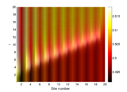
Figure 8: Time-dependent density in the right lead within the 2B approximation for a system with Fermi energy $\varepsilon_{F}=0$, and $\varepsilon_{0}=0.2$, $V_{\textrm{link}}=0.2$ and $U=0.6$). The system is driven out of equilibrium by an external bias $W_{L}=0.4$ and $W_{R}=0$. A density wave entering the lead can clearly be observed.

For times $t>t_{d}+T_{d}$ an equal amount of electrons enters in and exits from the interval, and a local steady-state is reached. The number of electrons in the considered interval is then given by

$$n_{s}N_{d}=n_{g}N_{d}+\int_{t_{d}}^{t_{d}+T_{d}}\!\!\!\!dt\,I_{d}(t)\sim n_{g}N_{d}+I_{s}T_{d},$$ (20)

with $I_{s}$ the value of the steady-state current. Taking into account that $T_{d}=N_{d}/v$ we conclude that the steady-state density deep inside the leads must be

$$n_{s}=n_{g}+I_{s}/v.$$ (21)

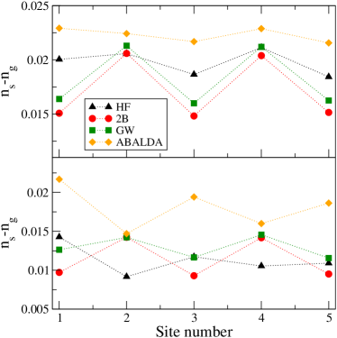
Figure 9: Difference between steady-state and ground-state density in the right lead for a system with Fermi energy $\varepsilon_{F}=0$, and $\varepsilon_{0}=0.2$, $V_{\textrm{link}}=0.2$ and for different values of the charging energy $U=0.6$ (top panel) and $U=1.4$ (bottom panel). The system is driven out of equilibrium by an external bias $W_{L}=0.4$ and $W_{R}=0$.

From Fig. 8 we see that for our 2B calculation the velocity $v$ has the value $v=1.88$. Given the value of the current of $I_{s}=0.034$ for this case ($U=0.6$) we find that the density difference $n_{s}-n_{g}$ is approximately $0.018$ which is in good agreement with the value in the upper panel of Fig. 9. Also for the case of the $U=1.4$ interaction strength we see from the lower panel of Fig. 9 that the ratio of the density differences $n_{s}-n_{g}$ for ABALDA and 2B is the same as the corresponding ratio for the currents in Fig. 7. We note that the value $v$ is close to the Fermi velocity in the lead at half-filling as obtained from a semi-classical calculation. This is given by $v=2V$. Equation (21) shows that if different approximations yield different values of the steady-state current they must also yield different values of the steady-state density deep inside the leads. This can indeed be seen in Fig. 9 where we plot $n_{s}-n_{g}$ for the various approximations for the first five sites in the right lead. The ordering of the density differences is identical to that of the currents in Fig. 7. Therefore, the ABALDA overestimates the difference between steady-state and ground state densities in the leads. However, ABALDA gives a quite good description of the density on the impurity site, comparable to those obtained within the many-body approximations. We thus conclude that the ABALDA xc-potential is quite accurate on the impurity site but that setting the potential to zero in the leads is a too crude approximation. As was discussed in relation to the Sham-Schlüter equation (see Eq. 19) the XC-potential will in general have values in the leads even when the interaction is localized on the impurity site only. Hence, in order to obtain accurate values for the current within a TDDFT approach one needs an XC-potential that has a nonzero value in the leads. We wish to observe that this nonlocality is different in nature from the non-local dependence of the XC-potential on the density. The latter is already implied by the conclusions of the previous section since non-locality in time and space are intimately related by conservation laws.

IV Conclusions and Outlook

We study electron transport through an interacting Anderson impurity model within TDDFT and MBPT frameworks. Results obtained in the ground-state, transient and steady-state regimes are compared with numerically exact tDMRG values.

In the ground state, we find that for large values of the on-site energy, the density obtained using the ABALDA XC-functional is close to the densities obtained within correlated MBPT approximations. However, for smaller values of the on-site energy, the difference between the ABALDA and the correlated MBPT densities is significant, ABALDA being closer to HF in this parameter range.

In all the cases where benchmark tDMRG results are available we find that the MBPT approximations beyond HF which we considered give densities and currents close to the benchmark ones for the entire parameter range considered. This is true for both the transient and steady-state regimes. We find that in particular the 2B approximation performs very well. The transients obtained within the 2B approximation are the closest to the tDMRG ones, while the HF and ABALDA transients deviate significantly. This indicates that it is important to include memory or retardation effects to properly describe quasi-particle scattering in non-equilbrium transport.

Regarding the TDDFT approach we find that the ABALDA performs very well and yields accurate densities on the interacting site but in many cases overestimates the steady-state currents. This problem can be linked to an overestimation of the lead-densities within the ABALDA. The results strongly suggest that it is necessary to go beyond the local approximation and that one especially needs to take into account XC-potentials that are nonlocal and that are non-zero within the leads. Improved functionals should therefore be nonlocal functionals in space. As has been clearly pointed out by Vignale VignaleKohn:96 , this implies that the functionals also need to be nonlocal in time in order to satisfy basic conservation laws. The construction of such functionals is a clear challenge for the future. One way to proceed would be to make connections to many-body theory with conserving approximations vonBarthetal2005 .

IV.1 Acknowledgements

Part of the calculations were performed at the CSC – IT Center for Science Ltd administered by the Ministry of Education, Science and Culture, Finland. Stefan Kurth acknowledges funding by the ”Grupos Consolidados UPV/EHU del Gobierno Vasco” (IT-319-07) and the European Community’s Seventh Framework Programme (FP7/2007-2013) under grant agreement No. 211956. Adrian Stan acknowledges funding by the Academy of Finland under grant no. 140327/2010. We acknowledge the support from the European Theoretical Spectroscopy Facility.

References

- (1) S. Datta, Electronics Transport in Mesoscopic Systems (Campridge University Press, New York, 1995).
- (2) M. Di Ventra, Electrical Transport in Nanoscale Systems (Cambridge University Press, 2008).
- (3) S. Gurviz and Y. Prager, Phys. Rev. B. 53, 15932 (1996).
- (4) G. Stefanucci and C.-O. Almbladh, Europhys. Lett. 67, 14 (2004).
- (5) V. Moldoveanu, V. Gudmundsson, and A. Manolescu, Phys. Rev. B 76, 165308 (2007).
- (6) P. Bokes, F. Corsetti, and R. W. Godby, Phys. Rev. Lett. 101, 046402 (2008).
- (7) D. Ryndyk, R. Gutierrez, B. Song, and G. Cuniberti, Green function techniques in the treatment of quantum transport at the molecular scale, in Energy Transfer Dynamics in Biomaterial Systems, edited by I. Burghardt, V. May, D. Micha, and E. Bittner, , Springer Series in Chemical Physics Vol. 93, p. 213, Springer-Verlag, 2009.
- (8) P. Myöhänen, A. Stan, G. Stefanucci, and R. van Leeuwen, Phys. Rev. B 80, 115107 (2009).
- (9) S. Andergassen, V. Meden, H. Schoeller, J. Splettstoesser, and M. Wegewijs, Nanotechnology 21, 272001 (2010).
- (10) X. Zheng et al., J. Chem. Phys. 133, 114101 (2010).
- (11) X. Zheng, F. Wang, C. Yam, Y. Mo, and G. Chen, Phys. Rev. B 75, 195127 (2007).
- (12) M. von Friesen, C. Verdozzi, and C. Almbladh, Phys. Rev. Lett. 103, 176404.
- (13) M. von Friesen, C. Verdozzi, and C. Almbladh, Phys. Rev. B 82, 155108 (2010).
- (14) A. Brandschädel, G. Schneider, and P. Schmitteckert, Annalen der Physik 522, 657 (2010).
- (15) S. Kurth, G. Stefanucci, C.-O. Almbladh, A. Rubio, and E. K. U. Gross, Phys. Rev. B 72, 035308 (2005).
- (16) E. Boulat, H. Saleur, and P. Schmitteckert, Phys. Rev. Lett. 101, 140601 (2008).
- (17) P. Myöhänen, A. Stan, G. Stefanucci, and R. van Leeuwen, Europhys. Lett. 84, 67001 (2008).
- (18) X. Wang, C. Spataru, M. Hybertsen, and A. Millis, Phys. Rev. B 77, 045119 (2008).
- (19) S. Schmitt and F. Anders, Phys. Rev. B 81, 165106 (2010).
- (20) U. Schollwöck, Rev. Mod. Phys. 77, 259 (2005).
- (21) C. Karrasch et al., Eur. Phys. Lett. 90, 30003 (2010).
- (22) C. Karrasch, M. Pletyukhov, L. Borda, and V. Meden, Phys. Rev. B 81, 125122 (2010).
- (23) W. Metzner, M. Salmhofer, C. Honerkamp, V. Meden, and K. Schönhammer, arXiv:1105.5289v1 [cond-mat.str-el] (2011).
- (24) F. Heidrich-Meisner, A. E. Feiguin, and E. Dagotto, Phys. Rev. B 79, 235336 (2009).
- (25) R. Dreizler and E. Gross, Density Functional Theory: An Approach to the Quantum Many-Body Problem (Springer-Verlag, New York, 1990).
- (26) M. Marques et al., Time-Dependent Density Functional Theory (Springer Heidelberg, 2006).
- (27) M. Di Ventra and T. Todorov, J.Phys: Condens.Matter 16, 8025 (2004).
- (28) F. Evers, F. Weigend, and M. Koentopp, Phys. Rev. B 69, 235411 (2004).
- (29) R. Baer, S. I. T. Seideman, and D. Neuhauser, J. Chem. Phys. 120, 3387 (2004).
- (30) G. Stefanucci and C.-O. Almbladh, Phys. Rev. B 69, 195318 (2004).
- (31) K. Burke, R. Car, and R. Gebauer, Phys. Rev. Lett. 94, 146803 (2005).
- (32) N. Sai, N. Bushong, R. Hatcher, and M. Di Ventra, Phys. Rev. B 75, 115410 (2007).
- (33) N. Sai, M. Zwolak, G. Vignale, and M. Di Ventra, Phys. Rev. Lett. 94, 186810 (2005).
- (34) G. Vignale and M. Di Ventra, Phys. Rev. B 79, 014201 (2009).
- (35) G. Vignale and W. Kohn, Phys. Rev. Lett. 77, 2037 (1996).
- (36) L.P. Kadanoff and G. Baym, Quantum Statistical Mechanics (Benjamin, New York, 1962).
- (37) P. Danielewicz, Ann. Phys. (New York) 152, 239 (1984).
- (38) G. Baym and L. Kadanoff, Phys. Rev. 124, 252 (1961).
- (39) G. Baym, Phys. Rev. 127, 1391 ((1962)).
- (40) K. Thygesen and A. Rubio, Phys. Rev. B 77, 115333 (2008).
- (41) M. Strange, C. Rostgaard, H. Häkkinen, and K. Thygesen, Phys. Rev. B 83, 115108 (2011).
- (42) M. Cini, Phys. Rev. B 22, 5887 (1980).
- (43) U. von Barth, N. Dahlen, R. van Leeuwen, and G. Stefanucci, Phys. Rev. B 72, 235109 (2005).
- (44) M. Hellgren and U. von Barth, Phys. Rev. B 78, 115107 (2008).
- (45) M. Hellgren and U. von Barth, J. Chem. Phys. 132, 044101 (2010).
- (46) P. W. Anderson, Phys. Rev. 124, 41 (1961).
- (47) R. van Leeuwen, N. E. Dahlen, G. Stefanucci, C.-O. Almbladh, and U. von Barth, Introduction to the keldysh formalism, in Time-Dependent Density Functional Theory, edited by M. Marques et al., , Lecture Notes in Physics Vol. 706, pp. 33–59, Springer-Verlag, 2006.
- (48) N. E. Dahlen, R. van Leeuwen, and A. Stan, Journal of Physics, Conf.Ser. 35, 340 (2006).
- (49) N. E. Dahlen and R. van Leeuwen, Phys. Rev. Lett. 98, 153004 (2007).
- (50) A. Stan, N. E. Dahlen, and R. van Leeuwen, J. Chem. Phys. 130, 224101 (2009).
- (51) A. Stan, N. E. Dahlen, and R. van Leeuwen, J. Chem. Phys. 130, 114105 (2009).
- (52) N. E. Dahlen and R. van Leeuwen, J. Chem. Phys. 122, 164102 (2007).
- (53) L. Hedin, Phys. Rev. 139, 796 (1965).
- (54) A. L. Fetter and J. D. Walecka, Quantum Theory of Many-Particle Systems (Dover Publications, 1971).
- (55) Y. Meir and N.S. Wingreen, Phys. Rev. Lett. 68, 2512 (1992).
- (56) N. Dahlen, A. Stan, and R. van Leeuwen, Journal of Physics, Conf.Ser. 35, 324 (2006).
- (57) A.-M. Uimonen, E. Khosravi, G. Stefanucci, S. Kurth, R. van Leeuwen, and E.K.U. Gross, Journal of Physics, Conf.Ser. 220, 012018 (2010).
- (58) P. Myöhänen, A. Stan, G. Stefanucci, and R. van Leeuwen, Journal of Physics, Conf.Ser. 220, 012017 (2010).
- (59) K. Schönhammer, O. Gunnarsson, and R. M. Noack, Phys. Rev. B 52, 2504 (1995).
- (60) N. A. Lima, M. F. Silva, L. N. Oliveira, and K. Capelle, Phys. Rev. Lett. 90, 146402 (2003).
- (61) C. Verdozzi, Phys. Rev. Lett. 101, 166401 (2008).
- (62) S. Kurth, G. Stefanucci, E. Khosravi, C. Verdozzi, and E.K.U. Gross, Phys. Rev. Lett. 104, 236801 (2010).
- (63) N. A. Lima, L. N. Oliveira, and K. Capelle, Europhys. Lett. 60, 601 (2002).
- (64) V. Franca, D. Vieira, and K. Capelle, arXiv:1102.5018 (2011).
- (65) R. van Leeuwen, Phys. Rev. Lett. 76, 3610 (1996).
- (66) S. Schenk, P. Schwab, M. Dzierzawa, and U. Eckern, Phys. Rev. B 83, 115128 (2011).
- (67) H. Mera, K. Kaasbjerg, Y. M. Niquet, and G. Stefanucci, Phys. Rev. B 81, 035110 (2010).