Effect of $Z_{b}$ states on $\Upsilon(3S)\to\Upsilon(1S)\pi\pi$ decays

Abstract

Within the framework of dispersion theory, we analyze the dipion transitions between the lightest $\Upsilon$ states, $\Upsilon(nS)\rightarrow\Upsilon(mS)\pi\pi$ with $m<n\leq 3$. In particular, we consider the possible effects of two intermediate bottomoniumlike exotic states $Z_{b}(10610)$ and $Z_{b}(10650)$. The $\pi\pi$ rescattering effects are taken into account in a model-independent way using dispersion theory. We confirm that matching the dispersive representation to the leading chiral amplitude alone cannot reproduce the peculiar two-peak $\pi\pi$ mass spectrum of the decay $\Upsilon(3S)\rightarrow\Upsilon(1S)\pi\pi$. The existence of the bottomoniumlike $Z_{b}$ states can naturally explain this anomaly. We also point out the necessity of a proper extraction of the coupling strengths for the $Z_{b}$ states to $\Upsilon(nS)\pi$, which is only possible if a Flatté-like parametrization is used in the data analysis for the $Z_{b}$ states.

I Introduction

The hadronic transitions $\Upsilon(nS)\to\Upsilon(mS)\pi\pi$ between $\Upsilon$ states of different radial excitation numbers $n$, $m$ are important processes for the understanding of systems with both heavy-quarkonium dynamics and low-energy QCD. Because of the large $b$ quark mass, bottomonia as nonrelativistic $b\bar{b}$ bound states are expected to be compact. The light hadrons such as pions emitted in the transitions between two bottomonia are normally expected to be due to the hadronization of soft gluons. Thus, the method of QCD multipole expansion together with soft-pion theorems Voloshin1980 ; Novikov1981 ; Kuang1981 ; Kuang2006 is often used to study these transitions. This means that such a method can be used to describe transitions where nonmultipole effects, such as coupled-channel effects and intermediate resonances, are small and the pions are very soft, such that the $\pi\pi$ final-state interaction (FSI) can be neglected. A characteristic of this method explored by the Cornell Cornell1978 ; Cornell1980 ; TMYan1980 and Orsay Orsay1973 ; Orsay1977:1 ; Orsay1977:2 groups is that the decay amplitudes are oscillatory functions of the decay momentum, which is a direct consequence of the radial node structure in the parent quarkonia wave functions. This can explain the ratio of partial decay widths $\Gamma(\Upsilon(3S)\to\Upsilon(1S)\pi\pi)/\Gamma(\Upsilon(2S)\to\Upsilon(1S)\pi\pi)\simeq 0.16$, though the phase space in the $\Upsilon(3S)\to\Upsilon(1S)\pi\pi$ process is much larger than that in $\Upsilon(2S)\to\Upsilon(1S)\pi\pi$, instead of interpretations of the initial quarkonia states as $B^{(*)}$–$\bar{B}^{(*)}$ molecules as in Ref. Glashow . The $\pi\pi$ mass spectra of the transitions between $2S$ and $1S$ heavy quarkonia can also be well described by such a method. However, there has been a well-known anomaly for the dipion transitions: the data for the decay $\Upsilon(3S)\to\Upsilon(1S)\pi\pi$ has a two-hump behavior, while a naive application of the formula Brown:1975dz that worked well for the $2S\to 1S$ and $3S\to 2S$ transitions would only give a single peak at large dipion invariant masses. Many mechanisms have been studied to explain this discrepancy, such as (i) coupled-channel effects with open-bottom intermediate states Lipkin1988 ; Kuang1991 ; Simonov2009 , (ii) the existence of a hypothetical resonance which couples to $\Upsilon\pi$ Voloshin1983 ; Zou1995 ; Guo2005 , (iii) the $\pi\pi$ resonance [the $f_{0}(500)$ or $\sigma$ meson] or strong $\pi\pi$ final-state interaction Komada1 ; Komada2 ; Uehara ; Moxhay1989 ; Chakravarty1994 ; Guo2005 ; Surovtsev2015 , (iv) relativistic corrections Voloshin2006 , etc. Among these mechanisms, the hypothetical $\Upsilon\pi$ resonance is in fact a tetraquark state with quark content $b\bar{b}q\bar{q}$ and quantum numbers $I^{G}(J^{P})=1^{+}(1^{+})$. The discovery of two $Z_{b}$ resonances in channels including both $\Upsilon(1S)\pi$ and $\Upsilon(3S)\pi$ by the Belle Collaboration in 2011 Belle2011:1 ; Belle2012:1 with such quantum numbers necessitates a reanalysis of $\Upsilon(3S)\to\Upsilon(1S)\pi\pi$, taking into account these resonances with their measured properties. Furthermore, since the dipion invariant mass reaches almost 900 MeV in such a decay, and the $\pi\pi$ $S$-wave FSI is known to be strong in this energy range, it is thus also necessary to account for the $\pi\pi$ FSI properly. Therefore, in the present paper we will use a formalism incorporating mechanisms (ii) and (iii) above, with (ii) upgraded to include the $Z_{b}$ states with measured properties given in the next paragraph, and (iii) such that the $\pi\pi$ FSI is treated in a model-independent way consistent with the $\pi\pi$ scattering data. The coupled-channel effects will be commented upon very briefly at the end of the paper; since we will use the leading-order heavy-quark expansion we will neglect any relativistic corrections.

The two charged bottomoniumlike resonances $Z_{b}(10610)^{\pm}$ and $Z_{b}(10650)^{\pm}$ were observed in the decay processes $\Upsilon(5S)\rightarrow\Upsilon(nS)\pi^{+}\pi^{-}$ ($n=1,2,3$) and $\Upsilon(5S)\rightarrow h_{b}(mP)\pi^{+}\pi^{-}$ ($m=1,2$) Belle2011:1 ; Belle2012:1 . Their quantum numbers are indeed $I^{G}(J^{P})=1^{+}(1^{+})$, and their masses and widths have been determined to be $M(Z_{b}(10610))=(10607.4\pm 2.0)\,\text{MeV}$, $\Gamma(Z_{b}(10610))=(18.4\pm 2.4)\,\text{MeV}$, and $M(Z_{b}(10650))=(10652.2\pm 1.5)\,\text{MeV}$, $\Gamma(Z_{b}(10650))=(11.5\pm 2.2)\,\text{MeV}$, respectively. Preliminary results for the branching fractions of $Z_{b}(10610)$ and $Z_{b}(10650)$ decays into $\Upsilon(nS)\pi^{+}$ ($n=1,2,3$) were also reported Belle2012:2 .

We will therefore study the decays $\Upsilon(nS)\rightarrow\Upsilon(mS)\pi\pi$ ($m<n\leq 3$), considering effects of the $Z_{b}$ states. We will use dispersion theory in the form of modified Omnès solutions to take into account the $\pi\pi$ FSIs. Herein, the $Z_{b}$-exchange amplitudes provide a left-hand-cut contribution to the dispersion integral. With the constraints of unitarity and analyticity, the decay amplitude is determined up to a few subtraction functions, which can be matched to the leading chiral tree-level amplitude in the low-energy region. We adopt the leading chiral Lagrangian for the coupling of two $S$-wave heavy quarkonia to an even number of pions from Ref. Mannel , constructed in the spirit of chiral perturbation theory and the heavy-quark nonrelativistic expansion. The theoretical framework is described in detail in Sec. II. In Sec. III, we fit the decay amplitudes to the data for the dipion transitions between two $\Upsilon(nS)$ states. Through fitting the experimental data of the $\pi\pi$ invariant mass distribution and the pion helicity angular distribution, the low-energy constants (LECs) in the chiral Lagrangian and the product of couplings for $Z_{b}\Upsilon\pi$ and $Z_{b}\Upsilon^{\prime}\pi$ [here we use $\Upsilon$ and $\Upsilon^{\prime}$ to refer to the $\Upsilon(nS)$ in the final and initial states, respectively] are determined. A brief summary and discussion will be presented in Sec. IV. Some details related to the matching of the dispersive representation as well as the Flatté parametrization are relegated to Appendixes A and B, respectively.

II Theoretical framework

II.1 Tree-level amplitudes

The decay amplitude for

$$\Upsilon(nS)(p_{a})\to\Upsilon(mS)(p_{b})\pi(p_{c})\pi(p_{d})$$ (1)

is described in terms of the Mandelstam variables

$$s =(p_{c}+p_{d})^{2},\qquad t=(p_{a}-p_{c})^{2}\,,\qquad u=(p_{a}-p_{d})^{2}\,,$$

$$3s_{0} \equiv s+t+u=m_{\Upsilon(nS)}^{2}+m_{\Upsilon(mS)}^{2}+2m_{\pi}^{2}\,.$$ (2)

For the $\pi^{+}\pi^{-}$ final state, the helicity angle $\theta$ is defined as the angle between the 3-momentum of the $\pi^{+}$ in the rest frame of the $\pi\pi$ system and that of the $\pi\pi$ system in the rest frame of the initial $\Upsilon(nS)$, where $\cos\theta\in[-1,1]$. The helicity angle for the $\pi^{0}\pi^{0}$ final state is defined similarly; however, due to the indistinguishability of the two neutral pions, we take $\cos\theta\in[0,1]$ CLEO2007 . $t$ and $u$ can be expressed in terms of $s$ and $\theta$ according to

$$t =\frac{1}{2}\left[3s_{0}-s+\kappa(s)\cos\theta\right]\,, u =\frac{1}{2}\left[3s_{0}-s-\kappa(s)\cos\theta\right]\,,$$

$$\kappa(s) \equiv\sigma_{\pi}\lambda^{1/2}\big{(}m_{\Upsilon(nS)}^{2},m_{\Upsilon(mS)}^{2},s\big{)}\,, \sigma_{\pi} \equiv\sqrt{1-\frac{4m_{\pi}^{2}}{s}}\,,$$ (3)

where $\lambda(a,b,c)=a^{2}+b^{2}+c^{2}-2(ab+ac+bc)$. We define $\mathbf{q}$ as the 3-momentum of the final vector meson in the rest frame of the initial state with

$$|\mathbf{q}|=\frac{1}{2m_{\Upsilon(nS)}}\lambda^{1/2}\big{(}m_{\Upsilon(nS)}^{2},m_{\Upsilon(mS)}^{2},s\big{)}\,.$$ (4)

The results of the QCD multipole expansion together with the soft-pion theorem can be reproduced by constructing a chiral effective Lagrangian for the $\Upsilon(nS)\to\Upsilon(mS)\pi\pi$ transition. Since the spin of the heavy quarks decouples in the heavy-quark limit, it is convenient to express the heavy quarkonia in term of spin multiplets, and one has $J\equiv\mathbf{\Upsilon}\cdot\boldsymbol{\sigma}+\eta_{b}$, where $\boldsymbol{\sigma}$ contains the Pauli matrices and $\mathbf{\Upsilon}$ and $\eta_{b}$ annihilate the $\Upsilon$ and $\eta_{b}$ states, respectively (see, e.g., Ref. Guo2011 ). For the contact $\Upsilon\Upsilon^{\prime}\pi\pi$ interaction, the effective Lagrangian to leading order in the chiral as well as the heavy-quark nonrelativistic expansion reads Mannel

$$\mathscr{L}_{\Upsilon\Upsilon^{\prime}\pi\pi}=\frac{c_{1}}{2}\langle J^{\dagger}J^{\prime}\rangle\langle u_{\mu}u^{\mu}\rangle+\frac{c_{2}}{2}\langle J^{\dagger}J^{\prime}\rangle\langle u_{\mu}u_{\nu}\rangle v^{\mu}v^{\nu}+\mathrm{h.c.}\,,$$ (5)

where $v^{\mu}=(1,\mathbf{0})$ is the velocity of the heavy quark. The pions as Goldstone bosons of the spontaneous breaking of the approximate chiral symmetry can be parametrized according to

$$u_{\mu}=i\left(u^{\dagger}\partial_{\mu}u\,-\,u\partial_{\mu}u^{\dagger}\right)\,,\qquad u^{2}=e^{i{\Phi}/{F_{\pi}}}\,,\qquad\Phi=\begin{pmatrix}\pi^{0}&\sqrt{2}{\pi^{+}}\\ \sqrt{2}{\pi^{-}}&-\pi^{0}\\ \end{pmatrix},$$ (6)

where $F_{\pi}=92.2\,\text{MeV}$ denotes the pion decay constant.

We need to define a $Z_{b}\Upsilon\pi$ interaction Lagrangian to calculate the contribution of the virtual intermediate $Z_{b}$ states, $\Upsilon(nS)\to Z_{b}\pi\to\Upsilon(mS)\pi\pi$. The leading-order term is proportional to the pion energy Guo2011 ,

$$\mathscr{L}_{Z_{b}\Upsilon\pi}=C_{Z}\Upsilon^{i}\langle{Z^{i}}^{\dagger}u_{\mu}\rangle v^{\mu}+\mathrm{h.c.}\,,$$ (7)

where

$$Z^{i}=\left({\begin{array}[]{*{2}c}\frac{1}{\sqrt{2}}Z^{0i}&Z^{+i}\\ Z^{-i}&-\frac{1}{\sqrt{2}}Z^{0i}\\ \end{array}}\right)\,.$$ (8)

In the following, we will use $Z_{b1}$ and $Z_{b2}$ to refer to $Z_{b}(10610)$ and $Z_{b}(10650)$, respectively, and use $C_{Z_{bi}\Upsilon(nS)\pi}$ to denote the coupling constants for the $Z_{bi}\Upsilon(nS)\pi$ vertices.

We briefly comment on the mass dimensions of the LECs and coupling constants in Eqs. (5) and (7). As the fields for the bottomonia and the $Z_{b}$ states are treated nonrelativistically, in principle they should be normalized in a nonrelativistic manner, leading to fields of mass dimension 3/2. The difference to the usual relativistic normalization is a factor of $\sqrt{M}$, with $M$ the mass of the heavy particle; since this difference is only a constant, we choose to absorb it into the definition of the coupling constants in the Lagrangians for simplicity, so that the heavy fields carry the usual relativistic normalization instead. Thus, the $c_{i}$ are dimensionless, while the $C_{Z}$ have mass dimension 1.

Note furthermore that, in order to preserve the analytic structure of the amplitudes exactly, we keep fully relativistic propagators for the $Z_{b}$ exchange graphs.

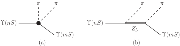
Figure 1: Tree diagrams relevant to the decays $\Upsilon(nS)\to\Upsilon(mS)\pi\pi$: (a) contact terms induced by the chiral Lagrangian; (b) $Z_{b}$ pole graphs. The crossed pole diagram is not shown explicitly.

The widths of the $Z_{b}$ states are of the order of $10\,\text{MeV}$ and are much smaller than the difference between the $Z_{b}$ masses and the $\Upsilon(nS)\pi$ thresholds. Thus, they can be safely neglected in the processes under investigation. Using the effective Lagrangians in Eqs. (5) and (7), the tree amplitude of the $\Upsilon(nS)\to\Upsilon(mS)\pi\pi$ processes as shown in Fig. 1 can be written as

$$\mathscr{M}^{\text{tree}}(s,t,u)=-\frac{4}{F_{\pi}^{2}}\epsilon_{\Upsilon(nS)}\cdot\epsilon_{\Upsilon(mS)}\Bigg{[}c_{1}p_{c}\cdot p_{d}+c_{2}p_{c}^{0}p_{d}^{0}+\sum_{i=1,2}\frac{C_{nm,i}}{2}\,p_{c}^{0}p_{d}^{0}\bigg{(}\frac{1}{t-m_{Z_{bi}}^{2}}+\frac{1}{u-m_{Z_{bi}}^{2}}\bigg{)}\Bigg{]},$$ (9)

where $\epsilon_{\Upsilon(nS)}$ and $\epsilon_{\Upsilon(mS)}$ are polarization vectors, $p_{c}^{0}$ and $p_{d}^{0}$ denote the energies of the pions in the lab frame, and $C_{nm,i}\equiv C_{Z_{bi}\Upsilon(nS)\pi}C_{Z_{bi}\Upsilon(mS)\pi}$ is the product of the coupling constants for the exchange of the $Z_{bi}$. Here, we have neglected terms suppressed by $p_{c}p_{d}/m_{Z_{bi}}^{2}$.

The partial-wave decomposition of $\mathscr{M}^{\text{tree}}$ can be easily performed by using Eq. (3) as well as the relation

$$p_{c}^{0}p_{d}^{0}=\frac{1}{4}\left(s+\mathbf{q}^{2}\right)-\frac{1}{4}\mathbf{q}^{2}\sigma_{\pi}^{2}\cos^{2}\theta\,.$$ (10)

In view of the following treatment of pion-pion FSIs using dispersive methods, it is useful to further decompose the partial waves into contact terms derived from the chiral Lagrangian Eq. (5), $M_{l}^{\chi}(s)$, and the projected $Z_{b}$-exchange terms, $\hat{M}_{l}(s)$, in the form

$$\mathscr{M}^{\text{tree}}(s,\cos\theta)=\epsilon_{\Upsilon(nS)}\cdot\epsilon_{\Upsilon(mS)}\sum_{l=0}^{\infty}\left[M_{l}^{\chi}(s)+\hat{M}_{l}(s)\right]P_{l}(\cos\theta)\,,$$ (11)

where $P_{l}(\cos\theta)$ are the standard Legendre polynomials. Since parity conservation (or isospin conservation combined with Bose symmetry) requires the pions to have even relative angular momentum $l$, only even partial waves contribute, and we only take into account the $S$- and $D$-wave components in this study, neglecting the effects of yet higher partial waves. Explicitly, the two parts of the $S$-wave projection of the tree amplitude read

$$M_{0}^{\chi}(s) =-\frac{2}{F_{\pi}^{2}}\bigg{\{}c_{1}\left(s-2m_{\pi}^{2}\right)+\frac{c_{2}}{2}\bigg{[}s+\mathbf{q}^{2}\Big{(}1-\frac{\sigma_{\pi}^{2}}{3}\Big{)}\bigg{]}\bigg{\}},$$ (12)

$$\hat{M}_{0}(s) =-\frac{2}{F_{\pi}^{2}\kappa(s)}\sum_{i=1,2}C_{nm,i}\Big{\{}\left(s+\mathbf{q}^{2}\right)Q_{0}(y_{i})-\mathbf{q}^{2}\sigma_{\pi}^{2}\left[y_{i}^{2}Q_{0}(y_{i})-y_{i}\right]\Big{\}}$$

$$\equiv\sum_{i=1,2}C_{nm,i}\,\bar{M}_{0i}(s)\,,$$ (13)

where $y_{i}\equiv(3s_{0}-s-2m_{Z_{bi}}^{2})/\kappa(s)$, and $Q_{0}(y)$ is a Legendre function of the second kind,

$$Q_{0}(y)=\frac{1}{2}\int_{-1}^{1}\frac{{\text{d}}z}{y-z}P_{0}(z)=\frac{1}{2}\log\frac{y+1}{y-1}\,.$$ (14)

The $D$-wave projections are given by

$$M_{2}^{\chi}(s) =\frac{2}{3F_{\pi}^{2}}c_{2}\mathbf{q}^{2}\sigma_{\pi}^{2}\,,$$ (15)

$$\hat{M}_{2}(s) =-\frac{5}{F_{\pi}^{2}\kappa(s)}\sum_{i=1,2}C_{nm,i}\left(s+\mathbf{q}^{2}-\mathbf{q}^{2}\sigma_{\pi}^{2}y_{i}^{2}\right)\left[(3y_{i}^{2}-1)Q_{0}(y_{i})-3y_{i}\right]$$

$$\equiv\sum_{i=1,2}C_{nm,i}\,\bar{M}_{2i}(s)\,.$$ (16)

II.2 Final-state interactions with dispersion relations

The $\pi\pi$ system undergoes strong FSIs in particular in the isospin-$0$ $S$-wave already at rather moderate energies above threshold, which has to be included in a theoretical calculation. A model-independent method to take FSIs into account is given by dispersion theory. Based on unitarity and analyticity, it determines the amplitudes up to certain subtraction constants, which can be obtained by matching to the results of chiral effective theory. For the processes $\Upsilon(nS)\to\Upsilon(mS)\pi\pi$ $(m<n\leq 3)$ studied here, the invariant mass of the pion pair is well below the $K\bar{K}$ threshold. Thus, it is not necessary to consider multichannel rescattering effects explicitly.

We write the partial-wave expansion of the full amplitude including the $\pi\pi$ FSI according to

$$\mathscr{M}^{\text{full}}(s,\cos\theta)=\epsilon_{\Upsilon(nS)}\cdot\epsilon_{\Upsilon(mS)}\sum_{l=0}^{\infty}\left[M_{l}(s)+\hat{M}_{l}(s)\right]P_{l}(\cos\theta)\,.$$ (17)

Here, $M_{l}(s)$ contains the right-hand cut and accounts for $s$-channel rescattering. On the other hand, $\hat{M}_{l}(s)$ represents (partial-wave projected) left-hand cut contributions, be it due to crossed-channel pole terms or rescattering effects. In the present study, we approximate the left-hand cuts by $Z_{b}$ exchange only. The functions $\hat{M}_{l}(s)$ are therefore given precisely by the expressions in Eqs. (13) and (16) already quoted in the previous section. By construction, they are real and free of discontinuities along the right-hand cut, such that in the regime of elastic $\pi\pi$ rescattering, the partial-wave unitarity conditions read

$$\textrm{Im}\,M_{l}(s)=\left[M_{l}(s)+\hat{M}_{l}(s)\right]\sin\delta_{l}^{0}(s)e^{-i\delta_{l}^{0}(s)}\,.$$ (18)

Below the inelastic threshold (here the $K\bar{K}$ threshold), the phases of the partial-wave amplitude $\delta_{l}^{0}$, of isospin $I=0$ and angular momentum $l$, coincide with the $\pi\pi$ elastic phase shifts, as required by Watson’s theorem Watson1 ; Watson2 . To solve Eq. (18), first we define the Omnès function Omnes ,

$$\Omega_{l}^{I}(s)=\exp\bigg{\{}\frac{s}{\pi}\int^{\infty}_{4m_{\pi}^{2}}\frac{{\text{d}}x}{x}\frac{\delta_{l}^{I}(x)}{x-s}\bigg{\}}\,,$$ (19)

which obeys $\Omega_{l}^{I}(s+i\epsilon)=e^{2i\delta_{l}^{I}}\Omega_{l}^{I}(s-i\epsilon)$. Then the discontinuity of the function $m_{l}(s)\equiv M_{l}(s)/\Omega_{l}^{0}(s)$ can be obtained with the help of Eq. (18) as

$$\frac{m_{l}(s+i\epsilon)-m_{l}(s-i\epsilon)}{2i}=\frac{M_{l}(s+i\epsilon)e^{-i\delta_{l}^{0}}-M_{l}(s-i\epsilon)e^{i\delta_{l}^{0}}}{2i|\Omega_{l}^{0}|}=\frac{\sin\delta_{l}^{0}\hat{M}_{l}}{|\Omega_{l}^{0}|}\,.$$ (20)

From the dispersion relation for the function $m_{l}(s)$, we then obtain the solution of Eq. (18) Leutwyler96

$$M_{l}(s)=\Omega_{l}^{0}(s)\bigg{\{}P_{l}^{n-1}(s)+\frac{s^{n}}{\pi}\int_{4m_{\pi}^{2}}^{\infty}\frac{{\text{d}}x}{x^{n}}\frac{\hat{M}_{l}(x)\sin\delta_{l}^{0}(x)}{|\Omega_{l}^{0}(x)|(x-s)}\bigg{\}}\,,$$ (21)

where the polynomial $P_{l}^{n-1}(s)$ is a subtraction function. In the absence of the inhomogeneous terms $\hat{M}_{l}(s)$ in the unitarity condition, i.e. without left-hand cuts, we would have found a standard Omnès solution for a form factor $P_{l}^{n-1}(s)\,\Omega_{l}^{I}(s)$, which is valid in the case where

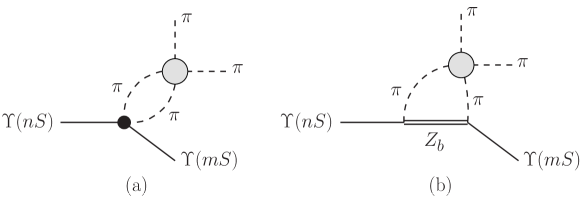
Figure 2: Pion-pion final-state interactions (a) with the two pions originating from a point source, denoted by the black dot, and (b) with pions produced by a $Z_{b}$ pole term. The gray blob denotes pion-pion rescattering.

the production of the two pions can be thought to originate from a point source; see Fig 2 (a). The modified solution in Eq. (21) contains a dispersion integral over the inhomogeneities $\hat{M}_{l}(s)$, which represents the rescattering including the production from a pole term, see Fig 2 (b), and provides the crossed-channel $Z_{b}$ exchange graph with the correct phase in accordance with Watson’s theorem. Very similar methods to include resonance exchange as an approximation to left-hand-cut structures have been applied recently to processes such as $\gamma\gamma\to\pi\pi$ Moussallam-gamma , $\eta\to\pi\pi\gamma$ KubisPlenter , or $B\to\pi\pi l\nu_{l}$ Kang .

In order to determine the necessary number of subtractions in Eq. (21), we need to make sure that the dispersive integral over the inhomogeneities converges, and hence have to investigate the high-energy behavior of the integrand. We first remark that for a phase shift $\delta_{l}^{I}(s)$ reaching $k\,\pi$ at high energies, the corresponding Omnès function falls off asymptotically as $s^{-k}$. Assuming that both the $S$-wave and $D$-wave $\pi\pi$ scattering phase shifts, $\delta_{0,2}^{0}(s)$, approach $\pi$ for high energies, we have $\Omega_{0,2}^{0}(s)\sim 1/s$ for large $s$. Second, we have checked that in an intermediate energy range of $1\,\text{GeV}^{2}\lesssim s\ll m_{\Upsilon}^{2}$, both inhomogeneities grow at most linearly in $s$. We conclude that in the dispersive representations for $M_{0}(s)$ and $M_{2}(s)$, three subtractions are sufficient to render the dispersive integrals convergent.

At low energies, i.e. close to or even below threshold, $M_{0}(s)$ and $M_{2}(s)$ can be matched to the chiral representation. We perform the matching in the limit of $\pi\pi$ rescattering being switched off, i.e. $\Omega_{l}^{0}(s)\equiv 1$, so that the subtraction functions can be identified exactly with the expressions given in Eqs. (12) and (15). As both $M_{0}^{\chi}(s)$ and $M_{2}^{\chi}(s)$ grow no faster than $\sim s^{2}$, the degree of the subtraction polynomial covers these terms. Therefore, the integral equations take the form

$$M_{0}(s) =\Omega_{0}^{0}(s)\bigg{\{}-\frac{2}{F_{\pi}^{2}}\bigg{[}c_{1}\left(s-2m_{\pi}^{2}\right)+\frac{c_{2}}{2}\bigg{(}s+\mathbf{q}^{2}\Big{(}1-\frac{\sigma_{\pi}^{2}}{3}\Big{)}\bigg{)}\bigg{]}$$

$$\qquad\qquad+\sum_{i=1,2}C_{nm,i}\frac{s^{3}}{\pi}\int_{4m_{\pi}^{2}}^{\infty}\frac{{\text{d}}x}{x^{3}}\frac{\bar{M}_{0i}(x)\sin\delta_{0}^{0}(x)}{|\Omega_{0}^{0}(x)|(x-s)}\bigg{\}}\,,$$

$$M_{2}(s) =\Omega_{2}^{0}(s)\bigg{\{}\frac{2}{3F_{\pi}^{2}}c_{2}\mathbf{q}^{2}\sigma_{\pi}^{2}+\sum_{i=1,2}C_{nm,i}\,\frac{s^{3}}{\pi}\int_{4m_{\pi}^{2}}^{\infty}\frac{{\text{d}}x}{x^{3}}\frac{\bar{M}_{2i}(x)\sin\delta_{2}^{0}(x)}{|\Omega_{2}^{0}(x)|(x-s)}\bigg{\}}\,.$$ (22)

A subtlety in this prescription concerns the kinematically singular parts of the subtraction functions $\propto 1/s$ that derive from the similarly singular inhomogeneities: the subtractions functions in Eq. (22) are not actually subtraction polynomials. These are an artifact of the partial-wave decomposition: the complete (polynomial) chiral amplitude as contained in Eq. (9) is obviously nonsingular, and due to $\Omega_{0}^{0}(0)=\Omega_{2}^{0}(0)=1$, this cancellation in the combination of partial waves is preserved in the dispersive representation. We show how to argue for the representation (22) more rigorously in Appendix A.

It is then straightforward to calculate the $\pi\pi$ invariant mass spectrum and helicity angular distribution for $\Upsilon(nS)\to\Upsilon(mS)\pi^{+}\pi^{-}$ using

$$\frac{{\text{d}}\Gamma}{{\text{d}}\sqrt{s}\,{\text{d}}\cos\theta}=\frac{\sqrt{s}\,\sigma_{\pi}|\mathbf{q}|}{128\pi^{3}m_{\Upsilon(nS)}^{2}}\left|M_{0}+\hat{M}_{0}+(M_{2}+\hat{M}_{2})P_{2}(\cos\theta)\right|^{2}\,,$$ (23)

where we have made use of $\sum_{\lambda,\lambda^{\prime}}\big{|}\epsilon_{\Upsilon(nS)}^{(\lambda)}\cdot\epsilon_{\Upsilon(mS)}^{(\lambda^{\prime})}\big{|}^{2}\approx 3$, which is an approximation accurate to a few per mil. For the neutral-pion process $\Upsilon(nS)\to\Upsilon(mS)\pi^{0}\pi^{0}$, Eq. (23) needs to be multiplied by $1/2$ in order to account for the indistinguishable neutral pions in the final state.

III Phenomenological discussion

We first discuss the $\pi\pi$ phase shifts used in the calculation of the Omnès functions and the dispersion integrals. As we describe the $S$-wave in a single-channel approximation, i.e. without taking inelasticities due to $K\bar{K}$ intermediate states into account explicitly, we employ the phase of the nonstrange pion scalar form factor (as determined in Ref. Hoferichter:2012wf from the solution of the coupled-channel Muskhelishvili–Omnès problem) instead of $\delta_{0}^{0}$, which yields a good description at least below the onset of the $K\bar{K}$ threshold. For the $D$-wave, we use the parametrization for $\delta_{2}^{0}$ given by the Madrid–Kraków collaboration Pelaez . Both phases are guided smoothly to the assumed asymptotic values $\delta_{0}^{0}(s),$ $\delta_{2}^{0}(s)\to\pi$ for $s\to\infty$. In practice, the dispersion integrals over the inhomogeneities in Eq. (22) are cut off at $s=(3\,\text{GeV})^{2}$; above that point, the phases are so close to $\pi$ already that the contributions to the dispersive integrals in Eq. (22) can be neglected.

All the LECs in the chiral Lagrangian Eq. (5) are unknown, and will be fitted to the experimental data for the $\Upsilon(nS)\to\Upsilon(mS)\pi\pi$ transitions. These LECs are different for processes with different values of $n$ and $m$, since there is no symmetry connecting different radial excitations of the bottomonium states. The experimental data that we will use include the $\pi\pi$ invariant mass distributions and the helicity angular distributions for the $\Upsilon(nS)\to\Upsilon(mS)\pi\pi$ $(m<n\leq 3)$ processes measured by the CLEO Collaboration in Ref. CLEO2007 . For the transitions from $\Upsilon(3S)$ to $\Upsilon(1S)$ and from $\Upsilon(2S)$ to $\Upsilon(1S)$, we simultaneously fit to the data of the $\pi^{0}\pi^{0}$ and the $\pi^{+}\pi^{-}$ final state. For the transition from $\Upsilon(3S)$ to $\Upsilon(2S)$, we only fit the data of the $\pi^{0}\pi^{0}$ final state due to the limited statistics of the $\Upsilon(3S)\to\Upsilon(2S)\pi^{+}\pi^{-}$ process (the event number is almost 1 order of magnitude smaller than the one for the $\pi^{0}\pi^{0}$ channel).

In principle, the $Z_{bi}\Upsilon(nS)\pi$ coupling strengths can be extracted from measuring the partial widths of both $Z_{b}$ states into $\Upsilon(nS)\pi$ $(n\leq 3)$ using

$$|C_{Z}|=\Bigg{\{}\frac{4\pi F_{\pi}^{2}m_{Z_{b}}^{2}\Gamma_{Z_{b}\to\Upsilon\pi}}{|\mathbf{p}_{f}|\big{(}m_{\pi}^{2}+\mathbf{p}_{f}^{2}\big{)}}\Bigg{\}}^{\frac{1}{2}},$$ (24)

where $|\mathbf{p}_{f}|\equiv\lambda^{1/2}\big{(}m_{Z_{b}}^{2},m_{\Upsilon}^{2},m_{\pi}^{2}\big{)}/(2m_{Z_{b}})$, and $\Gamma_{Z_{b}\to\Upsilon\pi}$ is the partial width for the $Z_{b}\to\Upsilon\pi$ decay. Thus, the coupling strengths can be obtained if the partial widths are known. In fact, there are preliminary results for the branching fractions of the decays of both $Z_{b}$ states into $\Upsilon(nS)\pi$ $(n\leq 3)$ Belle2012:2 , where the $Z_{b}$ line shapes were described using Breit–Wigner forms. All branching fractions are found to be of the order of a few per cent. If we naively calculated the partial widths by multiplying these branching fractions by the measured width of the $Z_{b}$ states, we would obtain

$$|C_{Z_{b1}\Upsilon(1S)\pi}^{\text{naive}}| =0.024\pm 0.003, |C_{Z_{b1}\Upsilon(2S)\pi}^{\text{naive}}| =0.23\pm 0.03, |C_{Z_{b1}\Upsilon(3S)\pi}^{\text{naive}}| =0.60\pm 0.08,$$

$$|C_{Z_{b2}\Upsilon(1S)\pi}^{\text{naive}}| =0.013\pm 0.002, |C_{Z_{b2}\Upsilon(2S)\pi}^{\text{naive}}| =0.11\pm 0.01, |C_{Z_{b2}\Upsilon(3S)\pi}^{\text{naive}}| =0.28\pm 0.03$$ (25)

(all in units of GeV), and the products of couplings relevant for the process $\Upsilon(3S)\to\Upsilon(1S)\pi\pi$ are

$$|C_{31,1}^{\text{naive}}|=(0.014\pm 0.004)\,\text{GeV}^{2},\qquad|C_{31,2}^{\text{naive}}|=(0.004\pm 0.001)\,\text{GeV}^{2}\,.$$ (26)

Here all the extractions are labeled by a superscript “naive” because this is not the appropriate way of extracting the coupling strengths in this case: the $Z_{b}$ structures are very close to the $B^{(*)}\bar{B}^{*}$ thresholds, and thus a Flatté parametrization should be used, which will lead to much larger partial widths into $\Upsilon\pi$ (and $h_{b}\pi$), and thus the relevant coupling strengths. As discussed in Appendix B, the sum of the partial widths of the $Z_{b}(10610)$ other than that for the $B\bar{B}^{*}$ channel should be larger than the nominal width, which is about $20\,\text{MeV}$. This would require at least some of the couplings to the $(b\bar{b})\pi$ channels to be significantly larger than the values indicated by naive calculation using branching fractions. Taking the $Z_{b}(10610)$ as an example, summing over all the $\Upsilon(nS)\pi\,(n=1,2,3)$ and $h_{b}(mP)\pi\,(m=1,2)$ branching fractions in Ref. Belle2012:2 gives about 14% or $3\,\text{MeV}$ in terms of partial widths. We therefore expect $|C_{Z_{b1}\Upsilon(nS)\pi}|^{2}$ to be roughly one order of magnitude larger than those from Eq. (III), and thus

$$|C_{31,1}|=\mathcal{O}(0.1\,\,\text{GeV}^{2})\,.$$ (27)

Figure 3: Simultaneous fit to the $\pi\pi$ invariant mass distributions and the helicity angle distributions in $\Upsilon(3S)\to\Upsilon(1S)\pi\pi$. The solid (dashed) and dotted (dot-dashed) curves show the best fit results without considering the $Z_{b}$ and using central values of the $Z_{bi}\Upsilon(nS)\pi$ couplings, given in Eq. (III), extracted from the $Z_{b}$ branching fractions. Solid and open circles refer to data points for the charged- and neutral-pion final states, respectively.

Because $\Upsilon(3S)\to\Upsilon(1S)\pi\pi$ is of particular interest for its unusual shape of the dipion invariant mass distribution, we will focus on this decay mode first. We try to fit to the dipion invariant mass distribution and the helicity angular distribution simultaneously without including any of the $Z_{b}$ states. The results of the best fit are shown as the solid (dashed) curves for the $\pi^{+}\pi^{-}$ ($\pi^{0}\pi^{0}$) mode in Fig. 3. It is obvious that the double-bump behavior of the invariant mass spectrum is not reproduced, although the angular distribution is described well. This calls for a new mechanism in addition to the $\pi\pi$ FSIs. We then include both $Z_{b}$ states. Since the coupling constants for the $Z_{b}\Upsilon\pi$ vertices extracted using the Flatté form are not available, we try to fix them to the central values in Eq. (26). The results are shown as the dotted (dot-dashed) curves in the same figure. Obviously, the best fits in both cases are very similar to each other.

It is interesting to see what happens if we treat the couplings of the $Z_{b}$ states to the $\Upsilon\pi$ as free parameters as well. However, the mass difference between the two $Z_{b}$ states, about only $40\,\text{MeV}$, is much smaller than the gap between their masses and the $\Upsilon(nS)\pi$ $(n=1,2,3)$ thresholds; they have the same quantum numbers and thus the same coupling structure as dictated by Eq. (7). It is therefore very difficult to distinguish their effects from each other in the processes under investigation. In practice, this means that the couplings for the $Z_{b}(10610)$ and $Z_{b}(10650)$ are strongly correlated in the fit and it is impossible to obtain a sensible uncertainty for them. Therefore, we use only one $Z_{b}$ state, by setting $C_{nm,2}=0$, and take its mass to be that of the $Z_{b}(10610)$. With three free parameters $c_{1}$, $c_{2}$, and $C_{31,1}$, we are able to achieve a very good agreement with the data for both the invariant mass and helicity angular distribution, as can be seen from the upper panel of Fig. 4.

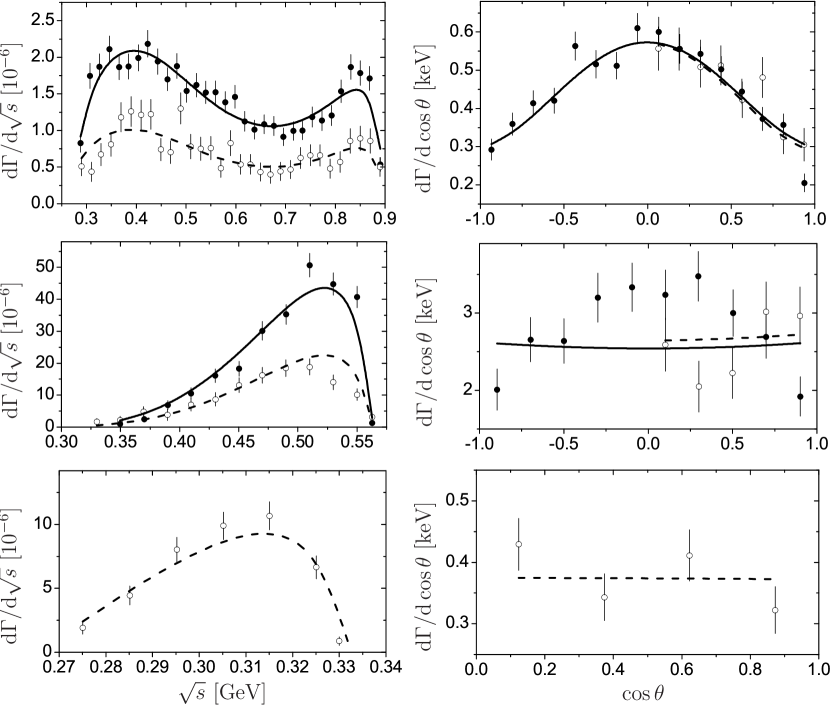
Figure 4: Fit results for the decays $\Upsilon(3S)\to\Upsilon(1S)\pi\pi$, $\Upsilon(2S)\to\Upsilon(1S)\pi\pi$, and $\Upsilon(3S)\to\Upsilon(2S)\pi^{0}\pi^{0}$ (from top to bottom). The left panels display the $\pi\pi$ invariant mass spectra, while the right panels show the $\cos\theta$ distributions. The solid and open circles denote the charged and neutral decay mode data, respectively; full and dashed lines show the theoretical fit results for charged- and neutral-pion final states.

In addition, the data for the processes $\Upsilon(2S)\to\Upsilon(1S)\pi\pi$ and $\Upsilon(3S)\to\Upsilon(2S)\pi\pi$ are also fitted, shown as the middle and lower panels in Fig. 4, respectively. It is not surprising that the invariant mass distributions for both of these two processes are described well, as their phase spaces are not large enough to allow for nontrivial structures comparable to the one for $\Upsilon(3S)\to\Upsilon(1S)\pi\pi$. Still, the agreement with the data for the angular distribution for $\Upsilon(2S)\to\Upsilon(1S)\pi\pi$ is not as good. This is mainly because of the discrepancy between the data for the modes with charged and neutral pions. This discrepancy was attributed to different efficiencies for reconstruction and resolutions, as well as the folding of the neutral angle in the experimental paper CLEO2007 , which are not available and thus not considered in our fit. The resulting values of the parameters as well as the $\chi^{2}$ per degree of freedom are shown in Table 1.

Table 1: The parameter results from the fits of the $\Upsilon(nS)\to\Upsilon(mS)\pi\pi$ processes. For the transitions from $\Upsilon(3S)$ to $\Upsilon(1S)$ and from $\Upsilon(2S)$ to $\Upsilon(1S)$, we simultaneously fit the data of the $\pi^{0}\pi^{0}$ final state and the $\pi^{+}\pi^{-}$ final state. For the transition from $\Upsilon(3S)$ to $\Upsilon(2S)$, we only fit the data of the $\pi^{0}\pi^{0}$ final state, due to the limited statistics of the $\Upsilon(3S)\to\Upsilon(2S)\pi^{+}\pi^{-}$ process.

	$~{}\Upsilon(3S)\to\Upsilon(1S)\pi\pi~{}$	$~{}\Upsilon(2S)\to\Upsilon(1S)\pi\pi~{}$	$~{}\Upsilon(3S)\to\Upsilon(2S)\pi^{0}\pi^{0}~{}$
$c_{1}$	$-0.025\pm 0.001$	$\phantom{-}0.09\pm 0.05$	$-0.6\pm 0.1$
$c_{2}$	$\phantom{-}0.026\pm 0.001$	$\phantom{-}0.04\pm 0.08$	$\phantom{-}0.2\pm 0.3$
$C_{nm,1}~{}[\text{GeV}^{2}]$	$\phantom{-}0.145\pm 0.006$	$\phantom{-}1.3\pm 1.4$	$\phantom{-}3.7\pm 2.6$
$\frac{\chi^{2}}{\rm d.o.f}$	$\frac{108.18}{87-3}=1.29$	$\frac{101.68}{40-3}=2.75$	$\frac{12.18}{11-3}=1.52$

Note that the fitting results are invariant under a sign change of all parameters simultaneously, as can be seen from Eq. (23). The resulting values of the LECs $c_{i}$ are very different for different transitions. These parameters are determined by short-distance physics, that is, the structure of the involved $\Upsilon(nS)$ states. Thus, such a difference may be explained by the node structures of different radial bottomonium excitations TMYan1980 ; Kuang1981 . We also notice that the node structure affects the coupling constants that are determined by the internal bottomonium structure but do not have an impact on the dipion invariant mass distribution.

We observe that the product of the $Z_{b}$ couplings to $\Upsilon(3S)\pi$ and $\Upsilon(1S)\pi$, $C_{31,1}$, is well constrained, while the values of $C_{21,1}$ and $C_{32,1}$ are consistent with zero (within 1.5 standard deviations for the latter). The value of $C_{31,1}$ extracted in this way is 1 order of magnitude larger than the naive value given in Eq. (26); however, it is of the same order as the expectation in Eq. (27). Notice that we have switched off the higher $Z_{b}$ in the fit, and thus the extracted coupling constant should be understood as containing effects from both $Z_{b}$ states.

Since the value of $C_{31,1}$ is well constrained, it is instructive to analyze different partial-wave components of the decay amplitude for $\Upsilon(3S)\to\Upsilon(1S)\pi\pi$. In Fig. 5, we plot the moduli of the $S$-wave and $D$-wave amplitudes from the $c_{i}$ terms and the $Z_{b}(10610)$ state for this process. Notice that, while the $c_{1}$ term is a pure $S$-wave, the $c_{2}$ term contributes to both $S$- and $D$-waves, and the $Z_{b}$-exchange in principle affects all partial waves. One observes that the $D$-wave contribution from the $Z_{b}$-exchange is much smaller than that from the $c_{2}$ term. This means that the curved behavior of the observed angular distribution is mainly due to the $c_{2}$ term. It should be mentioned that this observation is different from the one in Ref. Guo2005 , where the intermediate tetraquark state, analogous to the $Z_{b}$ here, is found to be dominant in the angular distribution. The reason is that in Ref. Guo2005 the mass of the tetraquark is fitted to $10.08\,\text{GeV}$, located between the masses of the $\Upsilon(3S)$ and $\Upsilon(1S)$ states. If we fix the $Z_{b}$ mass to such a low value, we indeed find that the ratio of the $D$- to $S$-wave components of the pure $Z_{b}$-exchange mechanism significantly increases. For the $S$-wave amplitudes, the contribution from the $c_{i}$ terms and that from the $Z_{b}$-exchange are of the same order, and both of them have a zero in the energy region of interest, responsible for the dip in the invariant mass distribution.

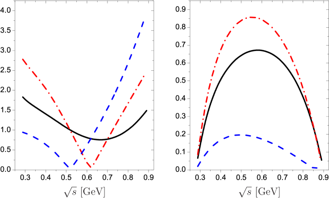
Figure 5: Moduli of the $S$- (left) and $D$-wave (right)amplitudes in the $\Upsilon(3S)\to\Upsilon(1S)\pi^{+}\pi^{-}$ process. The black solid lines represent our best fit results, while the red dot-dashed and blue dashed lines correspond to the contributions from the $c_{i}$ terms and the $Z_{b}(10610)$, respectively.

IV Conclusions

We have used dispersion theory to study FSIs in the decays $\Upsilon(nS)\to\Upsilon(mS)\pi\pi$, $(m<n\leq 3)$. In particular, we have analyzed the role of the $Z_{b}(10610)$ and $Z_{b}(10650)$ states in these transitions. Pion-pion FSIs have been considered in a model-independent way, and the leading chiral amplitude acts as the subtraction function in the modified Omnès solution. Through fitting the data of the $\pi\pi$ mass spectra and the angular $\cos\theta$ distributions, the couplings of the $\Upsilon\Upsilon^{\prime}\pi\pi$ vertex as well as the product of couplings of the $Z_{b}\Upsilon\pi$ vertex and the $Z_{b}\Upsilon^{\prime}\pi$ vertex are determined. We find that the $Z_{b}$ effects in $\Upsilon(2S)\to\Upsilon(1S)\pi\pi$ and $\Upsilon(3S)\to\Upsilon(2S)\pi^{0}\pi^{0}$ are very small, while they play a significant role in the $\Upsilon(3S)\to\Upsilon(1S)\pi\pi$ decay, which has a double-peak $\pi\pi$ mass spectrum. The product of couplings $C_{Z_{b1}\Upsilon(3S)\pi}C_{Z_{b1}\Upsilon(1S)\pi}$ obtained here is much larger than the one extracted naively from the branching fractions of the Breit–Wigner-parametrized $Z_{b}(10610)$ decays to $\Upsilon(nS)\pi^{+}(n=1,3)$ in Ref. Belle2012:2 . It is, however, consistent with a rough estimate based on a Flatté parametrization for the $Z_{b}(10610)$, which is in fact more appropriate for near-threshold states. This analysis calls for a detailed study for the partial widths of $Z_{b}(10610,10650)\to\Upsilon(1S,3S)\pi$ by analyzing the data for $\Upsilon(5S)\to\Upsilon(1S,3S)\pi\pi$, together with other processes where the $Z_{b}$ structures were observed, using, e.g., the formalism presented in Ref. Hanhart:2015cua .

Therefore, our results show the necessity to analyze the dipion decays of the $\Upsilon(nS)\,(n=3,4,5)$ states simultaneously, taking into account all the effects from $\pi\pi$ strong FSIs, the $Z_{b}$ states, and intermediate bottom mesons. The latter were neglected here because the $\Upsilon(3S)$ is well below the $B\bar{B}$ threshold and the left-hand-cut contribution due to the $Z_{b}(10610)$, located near the $B^{(*)}\bar{B}^{(*)}$ thresholds, could mimic the effects of the intermediate bottom mesons. Such a combined study, taking pion-pion final-state interactions into account consistently in the formalism laid out in this article, while allowing for more general intermediate states as left-hand-cut structures, should be pursued in the future. It would be most valuable to finally understand the peculiar behavior of the $\Upsilon(3S)\to\Upsilon(1S)\pi\pi$ decays on the one hand and to learn more about the $Z_{b}$ structures on the other.

Appendix A Singular inhomogeneities

The contribution $\propto c_{2}$ in the tree amplitude in Eq. (9) has the property of yielding $S$- and $D$-wave projections that diverge at $s=0$, while the combined expression is of course a polynomial in the Mandelstam variables $s$, $t$, and $u$: it can be written as (without changing the essence of the issue, we leave out all polarization vectors and overall prefactors such as coupling constants)

$$s +\mathbf{q}^{2}-\mathbf{q}^{2}\Big{(}1-\frac{4m_{\pi}^{2}}{s}\Big{)}\cos^{2}\theta=s+\mathbf{q}^{2}-\frac{1}{4m_{\Upsilon(nS)}^{2}}(t-u)^{2}$$

$$=s+\mathbf{q}^{2}+\frac{s^{2}}{4m_{\Upsilon(nS)}^{2}}-\frac{1}{2m_{\Upsilon(nS)}^{2}}\bigg{\{}\Big{[}t^{2}-3s_{0}t+\frac{9}{4}s_{0}^{2}\Big{]}+\Big{[}u^{2}-3s_{0}u+\frac{9}{4}s_{0}^{2}\Big{]}\bigg{\}}\,.$$ (28)

In the main text, we have claimed that these singular partial-wave projections can be included in a subtraction function of the Omnès representation, although these clearly do not constitute a subtraction polynomial. In this Appendix, we show how this can be justified.

The two terms in the curly brackets of Eq. (28) can be interpreted as (polynomial) $S$-wave amplitudes in the $t$- and $u$-channels of the decay. The projection of these onto $s$-channel partial waves yields additional contributions $\delta\hat{M}_{l}(s)$, $l=0,2$, to the hat functions, on top of the terms stemming from projected $Z_{b}$ pole terms. These additional contributions can be calculated easily:

$$\delta\hat{M}_{0}(s) \propto-\frac{1}{4m_{\Upsilon(nS)}^{2}}\int_{-1}^{1}{\text{d}}\cos\theta\bigg{\{}\Big{[}t^{2}-3s_{0}t+\frac{9}{4}s_{0}^{2}\Big{]}+\Big{[}u^{2}-3s_{0}u+\frac{9}{4}s_{0}^{2}\Big{]}\bigg{\}}=-\frac{\kappa^{2}(s)+3s^{2}}{12m_{\Upsilon(nS)}^{2}}\,,$$

$$\delta\hat{M}_{2}(s) \propto-\frac{5}{4m_{\Upsilon(nS)}^{2}}\int_{-1}^{1}{\text{d}}\cos\theta P_{2}(\cos\theta)\bigg{\{}\Big{[}t^{2}-3s_{0}t+\frac{9}{4}s_{0}^{2}\Big{]}+\Big{[}u^{2}-3s_{0}u+\frac{9}{4}s_{0}^{2}\Big{]}\bigg{\}}=-\frac{\kappa^{2}(s)}{6m_{\Upsilon(nS)}^{2}}.$$ (29)

We note that, with $s\ll m_{\Upsilon(nS)}^{2}$, the term $\propto s^{2}$ can be neglected, and we can use the approximation

$$\kappa^{2}(s)\approx(m_{\Upsilon(nS)}+m_{\Upsilon(mS)})^{2}\Big{[}(m_{\Upsilon(nS)}-m_{\Upsilon(mS)})^{2}-s\Big{]}\bigg{(}1-\frac{4m_{\pi}^{2}}{s}\bigg{)}\,,$$ (30)

such that the $\delta\hat{M}_{l}(s)$ only grow linearly with $s$ for large (but not too large to be comparable with the $\Upsilon$ masses) energies.

With a polynomial inhomogeneity, the dispersive integral can be performed analytically, using dispersive representations of the inverse of the Omnès function (see, e.g., Hoferichter ); we define

$$I_{n}(s)=-\frac{1}{\pi}\int_{4m_{\pi}^{2}}^{\infty}\frac{{\text{d}}x}{x^{n}}\frac{\sin\delta(x)}{|\Omega(x)|(x-s)}\,$$ (31)

and find

$$\Omega^{-1}(s) =1-s\,\dot{\Omega}(0)+s^{2}I_{2}(s)=1-s\,\dot{\Omega}(0)-\frac{s^{2}}{2}\big{[}\ddot{\Omega}(0)-2\dot{\Omega}^{2}(0)\big{]}+s^{3}I_{3}(s)$$

$$=1-s\,\dot{\Omega}(0)-\frac{s^{2}}{2}\big{[}\ddot{\Omega}(0)-2\dot{\Omega}^{2}(0)\big{]}-\frac{s^{3}}{6}\big{[}\dddot{\Omega}(0)-6\ddot{\Omega}(0)\dot{\Omega}(0)+6\dot{\Omega}^{3}(0)\big{]}+s^{4}I_{4}(s)$$ (32)

(assuming $\Omega(s)\sim 1/s$ for large $s$), which can be solved for the $I_{n}(s)$. The full contribution of the additional inhomogeneities to the partial-wave amplitudes is then given by

$$\delta\hat{M}(s)+\Omega(s)\frac{s^{3}}{\pi}\int_{4m_{\pi}^{2}}^{\infty}\frac{{\text{d}}x}{x^{3}}\frac{\delta\hat{M}(x)\sin\delta(x)}{|\Omega(x)|(x-s)}\,.$$ (33)

If we write $\delta\hat{M}(s)=m_{1}s+m_{0}+m_{-1}/s$, the terms involving $\Omega^{-1}(s)$ in the solutions of Eq. (A) for $I_{n}(s)$ exactly cancel $\delta\hat{M}(s)$. One ends up with a partial-wave contribution

$$\Omega(s) \bigg{\{}m_{1}s\big{(}1-s\,\dot{\Omega}(0)\big{)}+m_{0}\Big{(}1-s\,\dot{\Omega}(0)-\frac{s^{2}}{2}\big{[}\ddot{\Omega}(0)-2\dot{\Omega}^{2}(0)\big{]}\Big{)}$$

$$+\frac{m_{-1}}{s}\bigg{(}1-s\,\dot{\Omega}(0)-\frac{s^{2}}{2}\big{[}\ddot{\Omega}(0)-2\dot{\Omega}^{2}(0)\big{]}-\frac{s^{3}}{6}\big{[}\dddot{\Omega}(0)-6\ddot{\Omega}(0)\dot{\Omega}(0)+6\dot{\Omega}^{3}(0)\big{]}\bigg{)}\bigg{\}}$$

$$=\Omega(s)\big{\{}\delta\hat{M}(s)+[\text{quadratic subtraction~{}polynomial}]\big{\}}\,.$$ (34)

The first part acts as the subtraction function in the dispersion integral, including the singular term in $\kappa^{2}(s)$ $\propto 1/s$. The remainder—the subtraction terms obtained from derivatives of the Omnès function at zero—can be discarded based on arguments on the high-energy behavior in analogy to Appendix B of Ref. Kang .

Appendix B Flatté parametrization

In this Appendix, we briefly illustrate the effect of close-by thresholds on the apparent width of a resonance signal. To be specific, we will concentrate on the $Z_{b}(10610)$; yet, the discussion applies in general for any structure located very close to a strongly coupled threshold. Thus, a similar argument can also be used for the $Z_{b}(10650)$. The discussion is based on the Flatté parametrization Flatte and is not new. It has been emphasized in the case of the $f_{0}(980)$ Zou1993 (for discussions of the $f_{0}(980)/a_{0}(980)$ states using the Flatté formalism, see also Ref. Haidenbauer2005 ).

In addition to $B\bar{B}^{*}$, the $Z_{b}(10610)$ has several two-body decay channels such as $\Upsilon(nS)\pi$, $h_{b}(mP)\pi$, as well as the so-far unobserved $\eta_{b}\rho$. All these bottomonium channels have thresholds much lower than the $B\bar{B}^{*}$ one, and thus the sum of their partial widths can be approximated by a constant width $\Gamma_{1}$. Then the Flatté parametrization for the $Z_{b}$ spectral function is proportional to Flatte

$$\frac{1}{\big{|}{s-m_{Z_{b1}}^{2}}+im_{Z_{b1}}\left[\Gamma_{1}+\Gamma_{B\bar{B}^{*}}(s)\right]\big{|}^{2}}\,,$$ (35)

where

$$\Gamma_{B\bar{B}^{*}}(s)=\frac{g^{2}}{8\pi m_{Z_{b1}}^{2}}\left[k\,\theta(\sqrt{s}-m_{B}-m_{B^{*}})+i\,\kappa\,\theta(-\sqrt{s}+m_{B}+m_{B^{*}})\right]\,,$$ (36)

with $g$ the coupling constant of the $Z_{b1}B\bar{B}^{*}$ vertex, $k$ the center-of-mass momentum of the $B$ meson, and $\kappa=|k|$. It is easy to see that for either $\sqrt{s}>m_{B}+m_{B^{*}}$ or $\sqrt{s}<m_{B}+m_{B^{*}}$ the denominator in Eq. (35) becomes larger when $g$ increases. Therefore, if the pole is located very close to the $B\bar{B}^{*}$ threshold, which should be the case for the $Z_{b}(10610)$, a coupling to $B\bar{B}^{*}$ makes the $Z_{b}$ spectral function narrower than $\Gamma_{1}$.

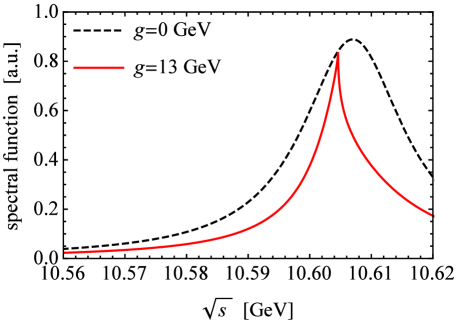
Figure 6: The spectral function of the $Z_{b}(10610)$ from Eq. (35). Here, $m_{Z_{b1}}=10.607\,\text{GeV}$ and $\Gamma_{1}=0.02\,\text{GeV}$ are used for illustration.

This can be seen from Fig. 6 where the spectral function of the $Z_{b}(10610)$ is shown in arbitrary units. Thus, we are led to conclude that $\Gamma_{1}$, the sum of the partial decay widths other than that into $B\bar{B}^{*}$, in the Flatté parametrization should be larger than the nominal width of the structure observed in the invariant mass distributions.

References

- (1) M. B. Voloshin and V. I. Zakharov, Phys. Rev. Lett. 45, 688 (1980).
- (2) V. A. Novikov and M. A. Shifman, Z. Phys. C 8, 43 (1981).
- (3) Y. P. Kuang and T. M. Yan, Phys. Rev. D 24, 2874 (1981).
- (4) Y. P. Kuang, Front. Phys. China 1, 19 (2006) [hep-ph/0601044].
- (5) E. Eichten, K. Gottfried, T. Kinoshita, K. D. Lane and T. M. Yan, Phys. Rev. D 17, 3090 (1978) [Phys. Rev. D 21, 313 (1980)].
- (6) E. Eichten, K. Gottfried, T. Kinoshita, K. D. Lane and T. M. Yan, Phys. Rev. D 21, 203 (1980).
- (7) T. M. Yan, Phys. Rev. D 22, 1652 (1980).
- (8) A. Le Yaouanc, L. Oliver, O. Pène and J. C. Raynal, Phys. Rev. D 8, 2223 (1973).
- (9) A. Le Yaouanc, L. Oliver, O. Pène and J.-C. Raynal, Phys. Lett. B 71, 397 (1977).
- (10) A. Le Yaouanc, L. Oliver, O. Pène and J. C. Raynal, Phys. Lett. B 72, 57 (1977).
- (11) A. De Rújula, H. Georgi and S. L. Glashow, Phys. Rev. Lett. 38, 317 (1977).
- (12) F.-K. Guo, P.-N. Shen and H.-C. Chiang, Phys. Rev. D 74, 014011 (2006) [hep-ph/0604252].
- (13) F.-K. Guo, P.-N. Shen, H.-C. Chiang and R.-G. Ping, Phys. Lett. B 658, 27 (2007) [hep-ph/0601120].
- (14) L. S. Brown and R. N. Cahn, Phys. Rev. Lett. 35, 1 (1975).
- (15) H. J. Lipkin and S. F. Tuan, Phys. Lett. B 206, 349 (1988).
- (16) H. Y. Zhou and Y. P. Kuang, Phys. Rev. D 44, 756 (1991).
- (17) Yu. A. Simonov and A. I. Veselov, Phys. Rev. D 79, 034024 (2009).
- (18) M. B. Voloshin, JETP Lett. 37, 69 (1983) [Pisma Zh. Eksp. Teor. Fiz. 37, 58 (1983)].
- (19) V. V. Anisovich, D. V. Bugg, A. V. Sarantsev and B. S. Zou, Phys. Rev. D 51, R4619 (1995).
- (20) F.-K. Guo, P.-N. Shen, H.-C. Chiang and R.-G. Ping, Nucl. Phys. A 761, 269 (2005) [hep-ph/0410204].
- (21) T. Komada, S. Ishida and M. Ishida, Phys. Lett. B 508, 31 (2001).
- (22) M. Ishida, S. Ishida, T. Komada and S. I. Matsumoto, Phys. Lett. B 518, 47 (2001).
- (23) M. Uehara, Prog. Theor. Phys. 109, 265 (2003) [hep-ph/0211029].
- (24) G. Bélanger, T. A. DeGrand and P. Moxhay, Phys. Rev. D 39, 257 (1989).
- (25) S. Chakravarty, S. M. Kim and P. Ko, Phys. Rev. D 50, 389 (1994) [hep-ph/9310376].
- (26) Y. S. Surovtsev, P. Bydžovský, T. Gutsche, R. Kamiński, V. E. Lyubovitskij and M. Nagy, Phys. Rev. D 91, 037901 (2015) [arXiv:1502.05368 [hep-ph]].
- (27) M. B. Voloshin, Phys. Rev. D 74, 054022 (2006) [hep-ph/0606258].
- (28) I. Adachi [Belle Collaboration], arXiv:1105.4583 [hep-ex].
- (29) A. Bondar et al. [Belle Collaboration], Phys. Rev. Lett. 108, 122001 (2012) [arXiv:1110.2251 [hep-ex]].
- (30) I. Adachi et al. [Belle Collaboration], arXiv:1209.6450 [hep-ex].
- (31) T. Mannel and R. Urech, Z. Phys. C 73, 541 (1997) [hep-ph/9510406].
- (32) D. Cronin-Hennessy et al. [CLEO Collaboration], Phys. Rev. D 76, 072001 (2007) [arXiv:0706.2317 [hep-ex]].
- (33) M. Cleven, F.-K. Guo, C. Hanhart and U.-G. Meißner, Eur. Phys. J. A 47, 120 (2011) [arXiv:1107.0254 [hep-ph]].
- (34) J. T. Daub, C. Hanhart and B. Kubis, J. High Energy Phys. 02 (2016) 009 [arXiv:1508.06841 [hep-ph]].
- (35) K. M. Watson, Phys. Rev. 88, 1163 (1952).
- (36) K. M. Watson, Phys. Rev. 95, 228 (1954).
- (37) R. Omnès, Nuovo Cim. 8, 316 (1958).
- (38) A. V. Anisovich and H. Leutwyler, Phys. Lett. B 375, 335 (1996) [hep-ph/9601237].
- (39) R. García-Martín and B. Moussallam, Eur. Phys. J. C 70, 155 (2010) [arXiv:1006.5373 [hep-ph]].
- (40) B. Kubis and J. Plenter, Eur. Phys. J. C 75, 283 (2015) [arXiv:1504.02588 [hep-ph]].
- (41) X.-W. Kang, B. Kubis, C. Hanhart and U.-G. Meißner, Phys. Rev. D 89, 053015 (2014) [arXiv:1312.1193 [hep-ph]].
- (42) M. Hoferichter, C. Ditsche, B. Kubis and U.-G. Meißner, J. High Energy Phys. 06 (2012) 063 [arXiv:1204.6251 [hep-ph]].
- (43) R. García-Martín, R. Kamiński, J. R. Peláez, J. Ruiz de Elvira, and F. J. Ynduráin, Phys. Rev. D 83, 074004 (2011) [arXiv:1102.2183 [hep-ph]].
- (44) C. Hanhart, Y. S. Kalashnikova, P. Matuschek, R. V. Mizuk, A. V. Nefediev and Q. Wang, Phys. Rev. Lett. 115, 202001 (2015) [arXiv:1507.00382 [hep-ph]].
- (45) M. Hoferichter, D. R. Phillips and C. Schat, Eur. Phys. J. C 71, 1743 (2011) [arXiv:1106.4147 [hep-ph]].
- (46) S. M. Flatté, Phys. Lett. B 63, 224 (1976).
- (47) B. S. Zou and D. V. Bugg, Phys. Rev. D 48, 3948 (1993).
- (48) V. Baru, J. Haidenbauer, C. Hanhart, A. E. Kudryavtsev, and U.-G. Meißner, Eur. Phys. J. A 23, 523 (2005) [nucl-th/0410099].