Exclusive Production of the $X(3872)$ in $B$ Meson Decay

Abstract

If the recently-discovered charmonium-like state $X(3872)$ is a loosely-bound S-wave molecule of the charm mesons $D^{0}\bar{D}^{*0}$ or $D^{*0}\bar{D}^{0}$, it can be produced through the weak decay of the $B$ meson into $D^{0}\bar{D}^{*0}K$ or $D^{*0}\bar{D}^{0}K$ followed by the coalescence of the charm mesons at a long-distance scale set by the scattering length of the charm mesons. The long-distance factors in the amplitude for the decay $B\to XK$ are determined by the binding energy of $X$, while the short-distance factors are essentially determined by the amplitudes for $B\to D^{0}\bar{D}^{*0}K$ and $B\to D^{*0}\bar{D}^{0}K$ near the thresholds for the charm mesons. We obtain a crude determination of the short-distance amplitudes by analyzing data from the Babar collaboration on the branching fractions for $B\to\bar{D}^{(*)}D^{(*)}K$ using a factorization assumption, heavy quark symmetry, and isospin symmetry. The resulting order-of-magnitude estimate of the branching fraction for $B^{+}\to XK^{+}$ is compatible with observations provided that $J/\psi\,\pi^{+}\pi^{-}$ is a major decay mode of the $X$. The branching fraction for $B^{0}\to XK^{0}$ is predicted to be suppressed by more than an order of magnitude compared to that for $B^{+}\to XK^{+}$.

I Introduction

The $X(3872)$ is a narrow charmonium-like resonance near 3872 MeV discovered by the Belle collaboration in electron-positron collisions through the $B$-meson decay $B^{\pm}\to XK^{\pm}$ followed by the decay $X\to J/\psi\,\pi^{+}\pi^{-}$ Choi:2003ue . This state has been confirmed by the CDF Acosta:2003zx and D0 Abazov:2004kp collaborations through its inclusive production in proton-antiproton collisions. The discovery mode $B^{\pm}\to XK^{\pm}$ has also been confirmed by the Babar collaboration Aubert:2004ns . The combined measurement of the mass of the $X$ is $3871.9\pm 0.5$ MeV Olsen:2004fp . The width of the $X$ is less than 2.3 MeV at 90% C.L. Choi:2003ue , which is much narrower than other charmonium states above the $D\bar{D}$ threshold. The product of the branching fractions associated with the discovery channel has been measured by the Belle and Babar collaborations: Choi:2003ue ; Aubert:2004ns ; Olsen:2004fp

$${\rm Br}[B^{+}\to XK^{+}]\,{\rm Br}[X\to J/\psi\,\pi^{+}\pi^{-}]=(1.3\pm 0.3)\times 10^{-5}.$$ (1)

The Belle collaboration recently observed the $X(3872)$ in a second decay mode: $X\to J/\psi\,\pi^{+}\pi^{-}\pi^{0}$ Abe:2004sd . The invariant mass distribution of the three pions is dominated by a virtual $\omega$ resonance. The branching ratio relative to the discovery decay channel is Abe:2004sd

$${{\rm Br}[X\to J/\psi\,\omega]\over{\rm Br}[X\to J/\psi\,\pi^{+}\pi^{-}]}=0.8\pm 0.3_{\rm stat}\pm 0.1_{\rm syst}.$$ (2)

Upper limits have been placed on the branching fractions for other decay modes of the $X$, including $D^{0}\bar{D}^{0}$, $D^{+}D^{-}$, $D^{0}\bar{D}^{0}\pi^{0}$ Abe:2003zv , $\chi_{c1}\gamma$, $\chi_{c2}\gamma$, $J/\psi\,\gamma$, $J/\psi\,\pi^{0}\pi^{0}$ Abe:2004sd , and $J/\psi\,\eta$ Aubert:2004fc . Upper limits have also been placed on the partial widths for the decay of $X(3872)$ into $e^{+}e^{-}$ Yuan:2003yz ; Metreveli:2004px and into $\gamma\gamma$ Metreveli:2004px .

The most plausible interpretations of the $X(3872)$ are a charmonium state with constituents $c\bar{c}$ Barnes:2003vb ; Eichten:2004uh ; Quigg:2004vf or a hadronic molecule with constituents $DD^{*}$ Tornqvist:2003na ; Voloshin:2003nt ; Wong:2003xk ; Braaten:2003he ; Swanson:2003tb ; Tornqvist:2004qy . Other proposed interpretations include an S-wave threshold enhancement in $D^{0}\bar{D}^{*0}$ scattering Bugg:2004sh , a “hybrid charmonium” state with constituents $c\bar{c}g$ Li:2004st , a vector glueball with a small admixture of charmonium states Seth:2004zb , and a diquark-antidiquark bound state with constituents $cu\bar{c}\bar{u}$ Maiani:2004vq . Measurements of the decays of the $X$ can be used to determine its quantum numbers and narrow down these options Close:2003sg ; Pakvasa:2003ea ; Rosner:2004ac ; Ko:2004cz . The charmonium options include members of the multiplet of the first radial excitation of P-wave charmonium and the multiplet of ground-state D-wave charmonium. The $h_{c}(2P)$, $\chi_{c0}(2P)$, and $\psi_{1}(1D)$, whose respective $J^{PC}$ quantum numbers are $1^{+-}$, $0^{++}$, and $1^{--}$, have already been ruled out as candidates for $X$. Evidence disfavoring each of the remaining states has been steadily accumulating Quigg:2004vf ; Olsen:2004fp .

The option of a $DD^{*}$ molecule is motivated by the proximity of the $X$ to the threshold for $D^{0}\bar{D}^{*0}$: $m_{D^{0}}+m_{D^{*0}}=3871.3\pm 1.0$ MeV. If $X$ is a $D^{0}\bar{D}^{*0}$/$D^{*0}\bar{D}^{0}$ molecule, its binding energy $E_{b}=m_{D^{0}}+m_{D^{*0}}-m_{X}$ is $E_{b}=-0.6\pm 1.1$ MeV. The central value corresponds to a resonance, but the error bar allows a bound state with $E_{b}>0$. The possibility that charm mesons might form molecular states was first considered some time ago Bander:1975fb ; Voloshin:ap ; DeRujula:1976qd ; Nussinov:1976fg . Tornqvist pointed out that $DD^{*}$ molecules were likely to be very loosely bound Tornqvist:1993ng . If the binding of $D^{0}\bar{D}^{*0}$ or $D^{*0}\bar{D}^{0}$ is due to pion exchange, the most favorable channels are S-wave with quantum numbers $J^{PC}=1^{++}$ and P-wave with quantum numbers $0^{-+}$ Tornqvist:1993ng ; Tornqvist:2003na ; Tornqvist:2004qy . In a model by Swanson that includes pion exchange at long distances and quark exchange at short distances, the only bound state is in the $1^{++}$ channel Swanson:2003tb . Another mechanism for generating a $DD^{*}$ molecule is the accidental fine-tuning of the mass of the $h_{c}(2P)$ or $\chi_{c1}(2P)$ to the $DD^{*}$ threshold which creates a molecule with quantum numbers $1^{+-}$ or $1^{++}$, respectively Braaten:2003he .

In the decay $X\to J/\psi\,\pi^{+}\pi^{-}\pi^{0}$, the invariant mass distribution of the three pions is dominated by a virtual $\omega$ resonance. In the decay $X\to J/\psi\,\pi^{+}\pi^{-}$, the invariant mass distribution of the two pions seems to peak near the upper endpoint Abe:2004sd , which suggests that they come from the decay of a virtual $\rho^{0}$ resonance. If the observed decay modes have been correctly interpreted as $X\to J/\psi\,\rho^{*}$ and $X\to J/\psi\,\omega^{*}$, the roughly equal branching fractions in Eq. (2) implies large isospin violations. This immediately rules out all charmonium options with the exceptions of $h_{c}(2P)$ and $\chi_{c1}(2P)$. These charmonium states are exceptional, because if either of their masses was somehow tuned sufficiently close to the $D^{0}\bar{D}^{*0}$ threshold, the resonant interactions with S-wave $DD^{*}$ scattering states would transform the charmonium state into a state that is predominantly a $DD^{*}$ molecule. If the $X(3872)$ is a loosely-bound $DD^{*}$ molecule, large isospin violations are expected. They arise simply from the fact that the mass of the $X$ is much closer to the $D^{0}\bar{D}^{*0}$ threshold than to the $D^{+}D^{*-}$ threshold at $3879.4\pm 1.0$ MeV.

The interpretation of $X(3872)$ as a loosely-bound $DD^{*}$ molecule has important implications for the production of the $X(3872)$ Braaten:2004rn ; Braaten:2004fk ; Braaten:2004jg ; Voloshin:2004mh . If the $X$ is a loosely-bound S-wave $D^{0}\bar{D}^{*0}$/$D^{*0}\bar{D}^{0}$ molecule, it can be produced in any high-energy collision that can create $D^{0}$ and $\bar{D}^{*0}$ or $D^{*0}$ and $\bar{D}^{0}$. If these charm mesons are produced with sufficiently small relative momentum, they can subsequently coalesce into the $X$. In Ref. Braaten:2004rn , this coalescence mechanism was applied to the exclusive decay process $\Upsilon(4S)\to Xh^{+}h^{-}$, where $h^{+}$ and $h^{-}$ are light hadrons. This decay can proceed through the decay of $\Upsilon(4S)$ into a virtual $B^{+}$ and a virtual $B^{-}$, followed by the decays $B^{+}\to\bar{D}^{0}h^{+}$ and $B^{-}\to D^{*0}h^{-}$ or by the decays $B^{+}\to\bar{D}^{*0}h^{+}$ and $B^{-}\to D^{0}h^{-}$, and then finally by the coalescence of the charm mesons into the $X$. Remarkably, the rate for this process can be calculated in terms of hadron masses and the width of the $B$ meson only. Unfortunately, it is many orders of magnitude too small to ever be observed in an experiment. The coalesence mechanism was applied to the discovery mode $B^{+}\to XK^{+}$ in Ref. Braaten:2004fk . An order-of-magnitude estimate of the branching fraction was found to be consistent with current experimental observations if the charge conjugation quantum number of the $X$ is $C=+$ and if $J/\psi\,\pi^{+}\pi^{-}$ is one of its major decay modes. It was pointed out that the molecular interpretation of the $X$ can be confirmed by the observation of a peak in the $D^{0}\bar{D}^{*0}$ invariant mass distribution just above the $D^{0}\bar{D}^{*0}$ threshold in the decay $B^{+}\to D^{0}\bar{D}^{*0}K^{+}$.

In this paper, we present a more thorough treatment of the coalesence mechanism for the production of $X$ in the exclusive decays $B\to XK$. We extend our previous work to the decay mode $B^{0}\to XK^{0}$, which has not yet been observed. Our analysis indicates that the branching fraction for $B^{0}\to XK^{0}$ should be suppressed relative to that for $B^{+}\to XK^{+}$ by more than an order of magnitude. A measurement or upper bound on the branching fraction for $B^{0}\to XK^{0}$ that is much smaller than that for $B^{+}\to XK^{+}$ would support the identification of the $X(3872)$ as a $DD^{*}$ molecule.

II Universality and the $\bm{X(3872)}$

The measurement of the mass of the $X$ indicates that its binding energy is likely to be within 1 MeV of the $D^{0}\bar{D}^{*0}$ threshold. This binding energy is small compared to the natural energy scale associated with pion exchange: $m_{\pi}^{2}/(2\mu_{DD^{*}})\approx 10$ MeV, where $\mu_{DD^{*}}$ is the reduced mass of the $D^{0}$ and $D^{*0}$. The unnaturally small binding energy $E_{b}$ implies that the S-wave $D^{0}\bar{D}^{*0}$ scattering length is large compared to the natural scale $1/m_{\pi}$. We assume that the $D^{0}\bar{D}^{*0}$/$D^{*0}\bar{D}^{0}$ system has a large scattering length $a$ in the $C=+$ channel and that the scattering length in the $C=-$ channel is negligible in comparison. The scattering lengths for elastic $D^{0}\bar{D}^{*0}$ scattering and for elastic $D^{*0}\bar{D}^{0}$ scattering are then both $a/2$. The large scattering length $a$ could be tuned to $+\infty$ by adjusting a short-distance parameter in QCD. One possible choice for this parameter is the mass of the up quark, since the precise value of the $D^{0}\bar{D}^{*0}$ threshold energy depends on this mass. Nonrelativistic few-body systems with short-range interactions and a large scattering length have universal properties that depend on the scattering length but are otherwise insensitive to details at distances small compared to $a$ Hammer:2004rn . Thus, the $D^{0}\bar{D}^{*0}$/$D^{*0}\bar{D}^{0}$ system will have universal properties that are insensitive to any of the shorter distance scales of QCD.

If the scattering length $a$ is large and positive, the simplest prediction of universality is that there is a loosely-bound 2-body bound state. In the case of the $D^{0}\bar{D}^{*0}$/$D^{*0}\bar{D}^{0}$ system, this bound state can be identified with the $X(3872)$. The universal formula for its binding energy is

$$E_{b}=\frac{1}{2\mu_{DD^{*}}a^{2}}.$$ (3)

The reduced mass $\mu_{DD^{*}}$ is well-approximated by

$$\mu_{DD^{*}}\simeq{m_{D^{0}}m_{D^{*0}}\over m_{X}}.$$ (4)

The wavefunction of the $X$ for $DD^{*}$ separations $r\gg 1/m_{\pi}$ is universal. The normalized wavefunction is

$$\psi(r)=(2\pi a)^{-1/2}{\exp(-r/a)\over r}.$$ (5)

Its Fourier transform is

$$\tilde{\psi}(q)=\frac{(8\pi/a)^{1/2}}{q^{2}+1/a^{2}}.$$ (6)

The momentum-space wavefunction has this universal form for $q\ll m_{\pi}$.

In the measurement of the binding energy, $E_{b}=-0.6\pm 1.1$ MeV, the central value is negative, corresponding to a resonance in $D^{0}\bar{D}^{*0}$ or $D^{*0}\bar{D}^{0}$ scattering rather than a bound state. The small negative binding energy requires a large negative scattering length. If this resonance was indeed the $X(3872)$, its dominant decay modes would be $D^{0}\bar{D}^{*0}$ and $D^{*0}\bar{D}^{0}$. After the subsequent decay of the $\bar{D}^{*0}$ or $D^{*0}$, the ultimate final state is $D^{0}\bar{D}^{0}\pi^{0}$ or $D^{0}\bar{D}^{0}\gamma$. The Belle collaboration has set an upper limit on the product of the branching fractions for $B^{+}\to XK^{+}$ and $X\to D^{0}\bar{D}^{0}\pi^{0}$ Abe:2003zv . Dividing by the central value of the corresponding product of branching fractions for the discovery mode, we obtain the limit

$${{\rm Br}[X\to D^{0}\bar{D}^{0}\pi^{0}]\over{\rm Br}[X\to J/\psi\pi^{+}\pi^{-}]}<5.$$ (7)

This loose upper bound seems to be the only quantitative evidence against the identification of $X(3872)$ as a $D^{0}\bar{D}^{*0}$/$D^{*0}\bar{D}^{0}$ resonance.

Throughout most of this paper, we will assume that $X$ is a $D^{0}\bar{D}^{*0}$/$D^{*0}\bar{D}^{0}$ bound state, which requires that $a$ be large and positive. The state of the $X$ can be written schematically as

$$|X\rangle={Z^{1/2}\over\sqrt{2}}\left(|D^{0}\bar{D}^{*0}\rangle+|D^{*0}\bar{D}^{0}\rangle\right)+\sum_{H}Z_{H}^{1/2}|H\rangle,$$ (8)

where $Z$ is the probability for the $X$ to be in the $D^{0}\bar{D}^{*0}$/$D^{*0}\bar{D}^{0}$ state, $Z_{H}$ is the probability for the $X$ to be in another hadronic state $H$, and $Z+\sum_{H}Z_{H}=1$. The other hadronic states $H$ could include charmonium states such as $\chi_{c1}(2P)$, scattering states of charm mesons such as $D^{+}D^{*-}$, and scattering states of a charmonium and a light hadron such as $J/\psi\,\rho$ or $J/\psi\,\omega$. Universality implies that $Z_{H}$ scales like $1/a$ and $Z$ approaches 1 as $a$ increases Braaten:2003he . In the limit $a\to\infty$, the state is a pure $D^{0}\bar{D}^{*0}$/$D^{*0}\bar{D}^{0}$ molecule.

The amplitudes for the scattering of $D^{0}\bar{D}^{*0}$ (or $\bar{D}^{0}D^{*0}$) with sufficiently small relative momentum are universal Braaten:2003he . If the $D^{0}$ and $\bar{D}^{*0}$ have momenta $\pm{\bm{q}}$ in the $DD^{*}$ rest frame with $|{\bm{q}}|\ll m_{\pi}$, the universal expressions for their amplitudes to scatter into $D^{0}\bar{D}^{*0}$ and $D^{*0}\bar{D}^{0}$ are

$${\cal A}[D^{0}\bar{D}^{*0}\to D^{0}\bar{D}^{*0}] = {8\pi m_{X}\over-1/a-iq},$$ (9a)

$${\cal A}[D^{0}\bar{D}^{*0}\to D^{*0}\bar{D}^{0}] = {8\pi m_{X}\over-1/a-iq}.$$ (9b)

We have implicitly assumed that the $D^{*}$ has the same polarization vector in the initial and final states. The numerator in Eqs. (9) differs from the product of the standard nonrelativistic factor $4\pi/\mu_{DD^{*}}$ and the relativistic normalization factor $4m_{D}m_{D^{*}}$ by a factor of $(1/\sqrt{2})^{2}$ from the projection of the initial and final $DD^{*}$ states onto the $C=+$ channel. The amplitudes for $D^{0}\bar{D}^{*0}$ or $D^{*0}\bar{D}^{0}$ with $|{\bm{q}}|\ll m_{\pi}$ to coalesce into $X$ are also universal Braaten:2003he :

$${\cal A}[D^{0}\bar{D}^{*0}\to X] = (16\pi m_{X}^{2}/\mu_{DD^{*}}a)^{1/2},$$ (10a)

$${\cal A}[D^{*0}\bar{D}^{0}\to X] = (16\pi m_{X}^{2}/\mu_{DD^{*}}a)^{1/2}.$$ (10b)

We have implicitly assumed that the $X$ has the same polarization vector as the $D^{*}$. Otherwise these amplitudes have an additional factor of $\epsilon_{X}^{*}\cdot\epsilon_{D^{*}}$. We have simplified the expressions for the amplitudes given in Ref. Braaten:2004rn by setting $Z=1$ and using the expression for the reduced mass in Eq. (4).

Any production process for $X$ necessarily involves a wide range of important momentum scales. In the decay $B\to XK$, the largest momentum scale is the mass $M_{W}\approx 80$ GeV of the $W$ boson that mediates the quark decay process $b\to c\bar{c}s$. The next largest momentum scale is $m_{b}-2m_{c}\approx 1.5$ GeV, which is the scale of the energy of the $s$ that recoils against the $c\bar{c}$ system. Then there is the scale $\Lambda_{\rm QCD}\approx 300$ MeV associated with the wavefunctions of light quarks in the hadrons and the scale $m_{\pi}\approx 140$ MeV associated with the pion-exchange interaction between the charm mesons. The smallest momentum scale is set by the wavefunction of the $DD^{*}$ molecule: $1/a<30$ MeV if $E_{b}<0.5$ MeV. This hierarchy of momentum scales can be summarized by the inequalities

$$1/a\ll m_{\pi}<\Lambda_{\rm QCD}\ll m_{b}-2m_{c}\ll M_{W}.$$ (11)

The two largest momentum scales, whose ratio is about 50, provides a very large hierarchy. It can be exploited by replacing the effects of the virtual $W$ by an effective weak hamiltonian that involves local interactions between quark fields. The two smallest momentum scales in Eq. (11) may also provide a very large hierarchy. The ratio $m_{\pi}a$ is greater than 4.3 if $E_{b}<0.5$ MeV and it could be much greater.

We can exploit the universality of nonrelativistic particles with large scattering lengths by introducing an ultraviolet cutoff $\Lambda$ on the relative momentum ${\bm{q}}$ of the $D^{0}$ or $\bar{D}^{0}$ in the $DD^{*}$ rest frame. If we choose this cutoff in the range

$$1/a\ll\Lambda\ll m_{\pi},$$ (12)

the behavior of $D^{0}\bar{D}^{*0}$ or $D^{*0}\bar{D}^{0}$ with $|{\bm{q}}|<\Lambda$ is governed by universality. We will refer to processes involving such small momenta as long-distance, while processes involving momenta satisfying $|{\bm{q}}|>\Lambda$ will be referred to as short-distance. In the next two sections, we apply this separation of scales to the decays $B\to D^{0}\bar{D}^{*0}K$ and $B\to XK$.

The ultraviolet momentum cutoff $\Lambda$ implies an ultraviolet energy cutoff $\Lambda^{2}/(2\mu_{DD^{*}})$. In the decomposition of $X$ in Eq. (8), all states $H$ for which the energy gap $|M_{H}-(m_{D^{0}}+m_{D^{*0}})|$ is greater than $\Lambda^{2}/(2\mu_{DD^{*}})$ can be excluded. The effects of such highly virtual states can be taken into account indirectly through the scattering length and through other effects on the $DD^{*}$ states. If $a$ is large enough, we can choose the ultraviolet energy cutoff $\Lambda^{2}/(2\mu_{DD^{*}})$ to be smaller than the smallest energy gap. In this case, only the $D^{0}\bar{D}^{*0}$ and $D^{*0}\bar{D}^{0}$ states in the decomposition in Eq. (8) remain and we can set $Z=1$.

The large $DD^{*}$ scattering length could arise from a fortuitous fine-tuning of the pion-exchange potential between $D^{0}$ and $\bar{D}^{*0}$ and between $D^{*0}$ and $\bar{D}^{0}$ in the $C=+$ channel. If $a>0$, there is necessarily a bound state near the $D^{0}\bar{D}^{*0}$ threshold, and it is identified with the $X$. Alternatively, the large scattering length could arise from a Feshbach resonance Hammer:2004rn , which requires the fine-tuning of the potential in a closed channel so that a bound state in that channel is close to the $D^{0}\bar{D}^{*0}$ threshold. If the closed channel is weakly coupled to $D^{0}\bar{D}^{*0}$ and $D^{*0}\bar{D}^{0}$ in the absence of the fine tuning, then the fine tuning generates a large scattering length when the bound state is extremely close to the $D^{0}\bar{D}^{*0}$ threshold. The natural choice for the closed channel is $c\bar{c}$, in which case the bound state in the closed channel could be the P-wave charmonium state $\chi_{c1}(2P)$. Since the decay of the $X(3872)$ seems to proceed through $J/\psi\,\rho^{*}$ and $J/\psi\,\omega^{*}$, one might be tempted to identify the closed channel responsible for the Feshbach resonance with $J/\psi\,\rho$ or $J/\psi\,\omega$. However the widths of the particles in the closed channel provides a lower bound on the width of the Feshbach resonance. The identification of the closed channel with $J/\psi\,\rho$ or $J/\psi\,\omega$ is therefore excluded by the fact that the widths of $\rho$ and $\omega$ are larger than the experimental upper bound on the width of the $X(3872)$.

III The Decay $\bm{B\to D^{0}{\bar{D}}^{*0}K}$

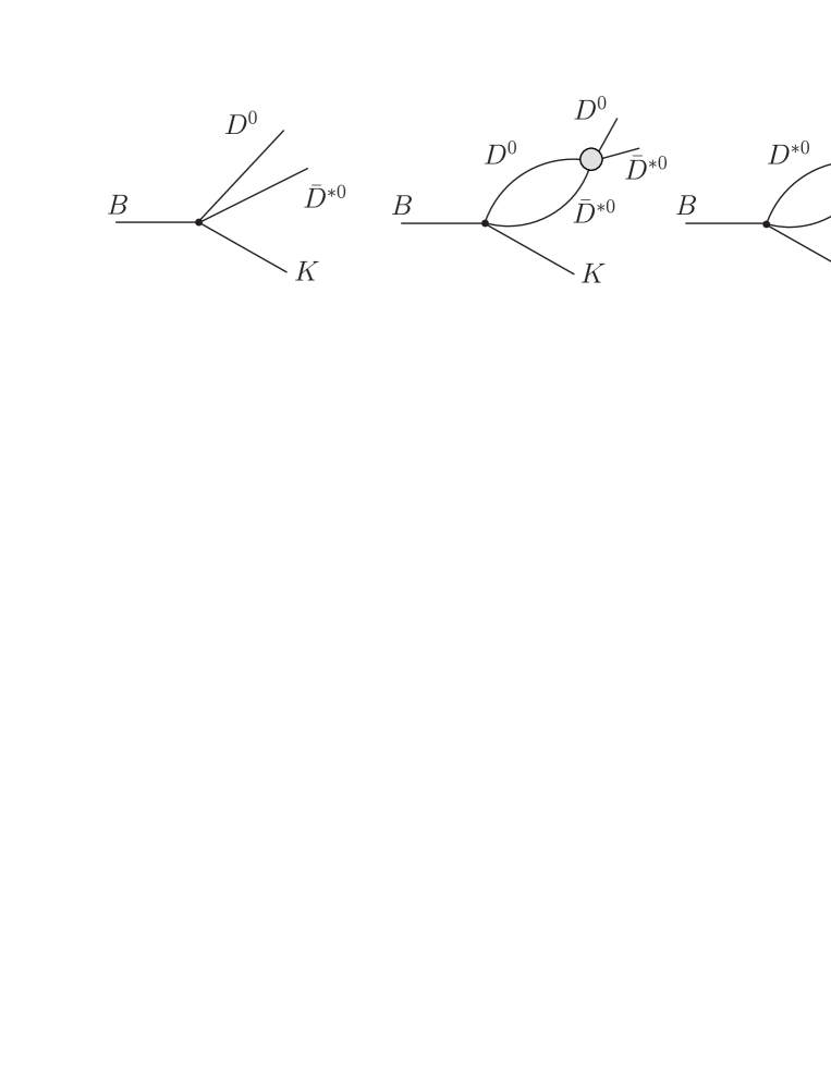
Figure 1: Feynman diagrams for the decay $B\to D^{0}\bar{D}^{*0}K$, with the short-distance decay amplitudes represented by dots and the long-distance scattering amplitudes represented by blobs.

We proceed to apply the separation of the long-distance scale $a$ from the shorter distance scales of QCD to the decay process $B\to D^{0}\bar{D}^{*0}K$. We denote the 4-momenta of the $B$, $D^{0}$, $\bar{D}^{*0}$, and $K$ by $P$, $q$, $q_{*}$, and $k$, respectively. We take the relative 3-momentum ${\bm{q}}=-{\bm{q}}_{*}$ in the $D^{0}\bar{D}^{*0}$ rest frame to be smaller than the separation scale $\Lambda$. The amplitude for $B\to D^{0}\bar{D}^{*0}K$ can be decomposed into three terms corresponding to the three diagrams in Fig. 1. The first diagram represents the direct production of $D^{0}\bar{D}^{*0}$ by the decay $B\to DD^{*}K$ at short distances. The second diagram represents the decay $B\to D^{0}\bar{D}^{*0}K$ at short distances followed by the elastic scattering of $D^{0}\bar{D}^{*0}$ at long distances. The third diagram represents the decay $B\to D^{*0}\bar{D}^{0}K$ at short distances followed by the scattering of $D^{*0}\bar{D}^{0}$ into $D^{0}\bar{D}^{*0}$ at long distances. The expression for the amplitude is

$${\cal A}[B\to D^{0}\bar{D}^{*0}K] = {\cal A}_{\rm short}[B\to D^{0}\bar{D}^{*0}K]$$ (13)

$$-i\int\!\!\frac{d^{4}\ell}{(2\pi)^{4}}\,{\cal A}_{\rm short}[B\to D^{0}\bar{D}^{*0}K]$$

$$\hskip 42.67912pt\times D(q+\ell,m_{D^{0}})\,D(q_{*}-\ell,m_{D^{*0}})\,{\cal A}[D^{0}\bar{D}^{*0}\to D^{0}\bar{D}^{*0}]$$

$$-i\int\!\!\frac{d^{4}\ell}{(2\pi)^{4}}\,{\cal A}_{\rm short}[B\to D^{*0}\bar{D}^{0}K]$$

$$\hskip 42.67912pt\times D(q+\ell,m_{D^{0}})\,D(q_{*}-\ell,m_{D^{*0}})\,{\cal A}[D^{*0}\bar{D}^{0}\to D^{0}\bar{D}^{*0}].$$

The propagators of the virtual $D$ and $D^{*}$ are

$$D(p,m)=(p^{2}-m^{2}+i\epsilon)^{-1}.$$ (14)

In the loop integrals, there is an implicit ultraviolet cutoff $|{\bm{\ell}}|<\Lambda$ on the 3-momenta of the virtual $D$ and $D^{*}$ in the $DD^{*}$ rest frame.

The long-distance scattering amplitudes in Eqs. (13) are given by the universal expressions in Eqs. (9). In the short-distance decay amplitudes in Eq. (13), we can neglect the relative 3-momentum ${\bm{\ell}}$ of the $D$ and $D^{*}$, since it is small compared to all the other momenta in the process. The 4-momenta of the $D$ and $D^{*}$ are well-approximated by $(m_{D^{0}}/m_{X})Q^{\mu}$ and $(m_{D^{*0}}/m_{X})Q^{\mu}$, where $Q=P-k$. Lorentz invariance then constrains the short-distance decay amplitudes to have the very simple forms

$${\cal A}_{\rm short}[B\to D^{0}\bar{D}^{*0}K] = c_{1}(\Lambda)\,P\cdot\epsilon^{*},$$ (15a)

$${\cal A}_{\rm short}[B\to D^{*0}\bar{D}^{0}K] = c_{2}(\Lambda)\,P\cdot\epsilon^{*},$$ (15b)

where $\epsilon$ is the polarization 4-vector of the $D^{*}$. The coefficients $c_{1}$ and $c_{2}$, which depend on the separation scale $\Lambda$, have dimensions of inverse energy.

In the loop integrals in Eq. (13), the integral over the variable $\ell_{0}$ can be evaluated by applying the residue theorem to the appropriate pole in one of the $D$ meson propagators:

$$\int\frac{d^{4}\ell}{(2\pi)^{4}}D(q+\ell,m_{D^{0}})\,D(q_{*}-\ell,m_{D^{*0}})={i\over 2m_{X}}\left({a\over 8\pi}\right)^{1/2}\int\frac{d^{3}\ell}{(2\pi)^{3}}\tilde{\psi}(\ell),$$ (16)

where $\tilde{\psi}(\ell)$ is the universal wavefunction of the $X$ given in Eq. (6). The remaining integral must be evaluated using the ultraviolet cutoff $|{\bm{\ell}}|<\Lambda$:

$$\int\frac{d^{3}\ell}{(2\pi)^{3}}\tilde{\psi}(\ell)=\left({2\over\pi^{3}a}\right)^{1/2}\left[\Lambda-{\arctan(a\Lambda)\over a}\right].$$ (17)

Putting all the ingredients together and keeping only the leading terms for $a\Lambda\gg 1$ in each of the three contributions, the decay amplitude in Eq. (13) reduces to

$${\cal A}[B\to D^{0}\bar{D}^{*0}K]\simeq\left(c_{1}(\Lambda)-{2a\Lambda[c_{1}(\Lambda)+c_{2}(\Lambda)]\over\pi(1+iaq)}\right)P\cdot\epsilon^{*}.$$ (18)

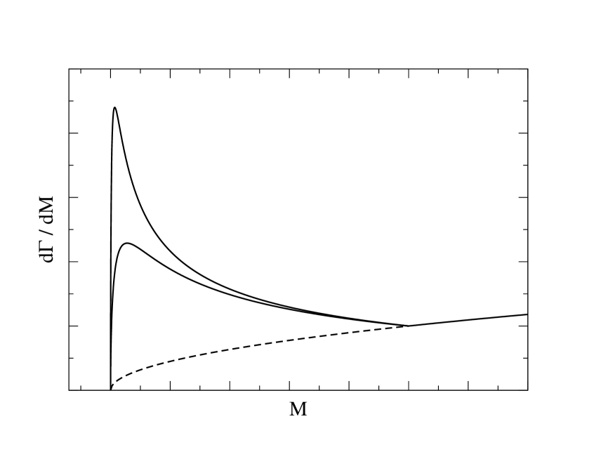
Figure 2: Invariant mass distribution for $D^{0}\bar{D}^{*0}$ near threshold (solid lines) for two values of the large scattering length that differ by a factor of 2. The peak in the invariant mass $M=m_{D^{0}}+m_{D^{*0}}+q^{2}/(2\mu_{DD^{*}})$ occurs at $q=1/a$. The crossover from the universal curves to the phase space distribution (dashed line) has been modeled by a sudden transition at $q=\Lambda_{\pi}$.

Our original expression for the decay amplitude in Eq. (13) simply corresponds to a separation of scales, so it is necessarily independent of the arbitrary scale $\Lambda$. However we have approximated the long-distance scattering amplitudes by ignoring terms suppressed by $1/(a\Lambda)$, in which case they reduce to the universal expressions in Eqs. (9). We have also approximated the short-distance amplitudes in Eqs. (15) by ignoring terms suppressed by $\ell/\Lambda$. Thus we can expect our expression for the amplitude in Eq. (18) to be independent of $\Lambda$ only up to terms that are suppressed by powers of $1/\Lambda$. This is possible only if the coefficients $c_{i}(\Lambda)$ scale like $1/\Lambda$, which implies that the combinations $\Lambda c_{i}(\Lambda)$ must approach ultraviolet fixed points $\hat{c}_{i}$ as $\Lambda$ increases. The approach to the fixed points is of course ultimately interrupted by the physical scale $m_{\pi}$. Neglecting terms that are suppressed by powers of $1/\Lambda$, the decay amplitude reduces to

$${\cal A}[B\to D^{0}\bar{D}^{*0}K]=-{2(\hat{c}_{1}+\hat{c}_{2})a\over\pi(1+iaq)}\,P\cdot\epsilon^{*}.$$ (19)

The resulting expression for the differential decay rate with respect to the $DD^{*}$ invariant mass $M$ is

$${d\Gamma\over dM}[B\to D^{0}\bar{D}^{*0}K]=|\hat{c}_{1}+\hat{c}_{2}|^{2}{\lambda^{3/2}(m_{B},m_{X},m_{K})\over 64\pi^{5}m_{B}^{3}m_{X}^{2}}\,{a^{2}q\over 1+a^{2}q^{2}},$$ (20)

where $q$ is the momentum of the $D$ or $D^{*}$ in the $DD^{*}$ rest frame,

$$q={\lambda^{1/2}(M,m_{D^{0}},m_{D^{*0}})\over 2M},$$ (21)

and $\lambda(x,y,z)$ is the triangle function:

$$\lambda(x,y,z)=x^{4}+y^{4}+z^{4}-2(x^{2}y^{2}+y^{2}z^{2}+z^{2}x^{2}).$$ (22)

Although we assumed $a>0$ in the derivation, our final result in Eq. (20) is valid for either sign of $a$. If $a<0$, the only difference in the derivation is that the integral in Eq. (16) cannot be interpreted in terms of a universal bound-state wavefunction, since there is no bound state. Near the threshold, the $DD^{*}$ invariant mass can be approximated by

$$M\simeq m_{D^{0}}+m_{D^{*0}}+q^{2}/(2\mu_{DD^{*}}).$$ (23)

The invariant mass distribution in Eq. (20) has a peak at $q=1/|a|$ with a height that scales like $|a|$ as $|a|$ increases. It decreases to half the maximum at $q=(2\pm\sqrt{3})/|a|$. The full width in $M$ at half maximum is $4\sqrt{3}/(\mu_{DD^{*}}a^{2})$.

The decay rate for $B\to D^{*0}\bar{D}^{0}K$ also proceeds by the Feynman diagrams in Fig. 1, except that the charm mesons in the final state are $D^{*0}$ and $\bar{D}^{0}$. The differential decay rate for $B\to D^{*0}\bar{D}^{0}K$ in the scaling region $q\ll m_{\pi}$ is given by exactly the same universal expression in Eq. (20). If the large scattering length occurred in the channel with charge conjugation $C=-$, the only difference would be that the factor $|\hat{c}_{1}+\hat{c}_{2}|^{2}$ in Eq. (20) would be replaced by $|\hat{c}_{1}-\hat{c}_{2}|^{2}$. We have not specified the charge of the $B$ meson. The fixed-point coefficients $\hat{c}_{1}$ and $\hat{c}_{2}$ in Eq. (20) have different values for the decays $B^{+}\to D^{0}\bar{D}^{*0}K^{+}$ and $B^{0}\to D^{0}\bar{D}^{*0}K^{0}$.

The expression for the differential decay rate in Eq. (20) applies only in the scaling region $q\ll m_{\pi}$. At larger values of $q$ that are still small compared to the scale $m_{b}-2m_{c}$, the resonant terms disappear and the decay amplitude reduces to the short-distance term $c_{1}(\Lambda)P\cdot\epsilon^{*}$ in Eqs. (15a). The corresponding invariant mass distribution $d\Gamma/dM$ for $q$ just above the scaling region follows the phase space distribution, which is proportional to $q$ in the limit $q\to 0$. The crossover from the resonant distribution proportional to $a^{2}q/(1+a^{2}q^{2})$ to the phase space distribution proportional to $q$ occurs at a momentum scale that we will denote by $\Lambda_{\pi}$. We expect $\Lambda_{\pi}$ to be comparable to $m_{\pi}$. Just above the crossover region, the differential decay rate can be approximated by

$${d\Gamma\over dM}[B\to D^{0}\bar{D}^{*0}K]\approx|c_{1}(\Lambda_{\pi})|^{2}{\lambda^{3/2}(m_{B},m_{X},m_{K})\over 256\pi^{3}m_{B}^{3}m_{X}^{2}}\,q.$$ (24)

A crude model of the crossover from the phase space distribution in Eq. (24) to the resonant distribution in Eq. (20) is a sudden but continuous transition at $q=\Lambda_{\pi}$, as illustrated in Figure 2. This requires

$$|c_{1}(\Lambda_{\pi})|\approx{2|\hat{c}_{1}+\hat{c}_{2}|\over\pi\Lambda_{\pi}}.$$ (25)

The integral of $d\Gamma/dM$ over the region $0<q<\Lambda_{\pi}$ increases with $a$. In the limit $a\to\infty$, it is 3 times larger than the integral of a phase space distribution normalized to the same value at $q=\Lambda_{\pi}$.

The Babar collaboration has measured the branching fractions for $B\to D^{0}\bar{D}^{*0}K$ and $B\to D^{*0}\bar{D}^{0}K$ using a data sample of about $8\times 10^{7}$ $B\bar{B}$ events Aubert:2003jq . The strongest signal was observed in the channel $B^{+}\to D^{*0}\bar{D}^{0}K^{+}$: $221\pm 27$ events above the background, but with a contamination of about 37 events due to crossfeed from other decay channels. If the invariant mass distributions could be measured with resolution much better than $m_{\pi}^{2}/(2\mu_{DD^{*}})\simeq 10$ MeV and if the histograms included enough events, one could actually resolve the resonant enhancement near threshold that is illustrated in Figure 2 and determine both $a$ and $|\hat{c}_{1}+\hat{c}_{2}|^{2}$ directly from the data. The resolution that would be required may not be out of the question, since Babar has presented a histogram of $d\Gamma/dM$ for the decay $B^{0}\to D^{*-}\bar{D}^{*0}K^{+}$ with 20 MeV bins Aubert:2003jq . However the region $q<m_{\pi}$ in which the enhancement is expected to occur accounts for only about $0.2$% of the available phase space for the decay $B\to D^{0}\bar{D}^{*0}K$. Even with an enhancement in this region by a factor of 3 from a very large scattering length, it may be difficult to accumulate enough events in this region to resolve the structure in Figure 2.

IV The Decay $\bm{B\to XK}$

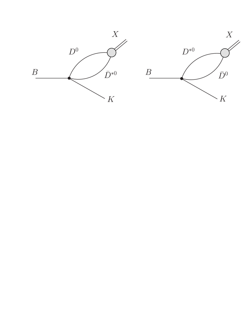
Figure 3: Feynman diagrams for the decay $B\to XK$, with the short-distance decay amplitudes represented by dots and the long-distance coalesence amplitudes represented by blobs.

We proceed to apply the separation of the long-distance scale $a$ from the shorter distance scales of QCD to the decay process $B\to XK$. The amplitude for $B\to XK$ can be decomposed into two terms corresponding to the two diagrams in Fig. 3. The first diagram represents the decay $B\to D^{0}\bar{D}^{*0}K$ at short distances followed by the coalescence of $D^{0}\bar{D}^{*0}$ into $X$ at long distances. The second diagram represents the decay $B\to D^{*0}\bar{D}^{0}K$ at short distances followed by the coalescence of $D^{*0}\bar{D}^{0}$ into $X$ at long distances. We denote the 4-momenta of the $B$, $X$, and $K$ by $P$, $Q$, and $k$, respectively. The expression for the amplitude is

$${\cal A}[B\to XK] = -i\int\!\!\frac{d^{4}\ell}{(2\pi)^{4}}\,{\cal A}_{\rm short}[B\to D^{0}\bar{D}^{*0}K]$$ (26)

$$\hskip 42.67912pt\times D(q+\ell,m_{D^{0}})\,D(q_{*}-\ell,m_{D^{*0}})\,{\cal A}[D^{0}\bar{D}^{*0}\to X]$$

$$-i\int\!\!\frac{d^{4}\ell}{(2\pi)^{4}}\,{\cal A}_{\rm short}[B\to D^{*0}\bar{D}^{0}K]$$

$$\hskip 42.67912pt\times D(q+\ell,m_{D^{0}})\,D(q_{*}-\ell,m_{D^{*0}})\,{\cal A}[D^{*0}\bar{D}^{0}\to X],$$

where $q^{\mu}=(m_{D^{0}}/m_{X})Q^{\mu}$ and $q_{*}^{\mu}=(m_{D^{*0}}/m_{X})Q^{\mu}$ are 4-momenta that add up to the 4-momentum $Q^{\mu}$ of the $X$.

One might ask why we do not include the diagram in Fig. 4(a), which represents the direct production of $X$ through the decay $B\to HK$ at short distances, where $H$ is one of the hadronic states that appears in the schematic decomposition of the wavefunction of $X$ in Eq. (8). Such a short-distance term could be expressed in the form $Z_{H}^{1/2}{\cal A}_{\rm short}[B\to HK]$ and can be interpreted as a contribution from a “core component” of the $X$ Voloshin:2004mh . The reason such a diagram need not be considered is that it is already taken into account through the diagrams in Fig. 3. The various components of the wavefunction for the bound state $X$ satisfy coupled integral equations. By iterating the integral equations, one can always eliminate the component $H$ in terms of a $DD^{*}$ component. Thus the diagram in Fig. 4(a) can be expressed in terms of diagrams with explicit $DD^{*}$ states as in Figs. 4(b) and (c). In the separation of the amplitude into short-distance parts and long-distance parts represented by Fig. 3, the propagators for $H$ in Figs. 4(b) and (c) are absorbed into the short-distance decay amplitude.

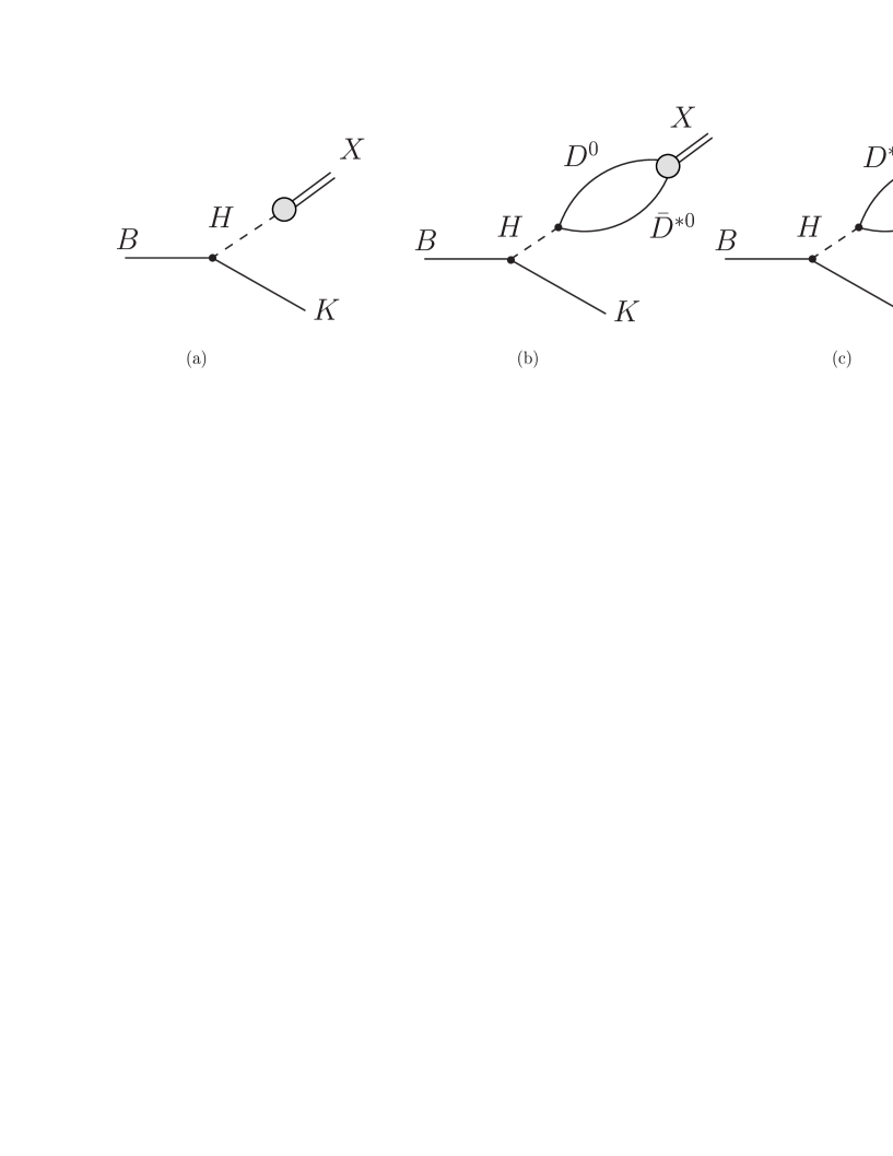
Figure 4: Feynman diagrams for the decay $B\to XK$: (a) the diagram corresponding to the production of the hadron $H$ at short distances, with the blob representing the probability factor $Z_{H}^{1/2}$, (b)–(c) equivalent diagrams obtained by iterating the bound-state equation to get $DD^{*}$ components of the wavefunction.

The long-distance coalescence amplitudes in Eq. (26) are given by the universal expressions in Eqs. (10). The short-distance amplitudes for the decays into $DD^{*}K$ are given in Eqs. (15). The loop integrals in Eq. (26) can be evaluated as in Eqs. (16) and (17). If we keep only the leading terms for $a\Lambda\gg 1$, the amplitude has a factor $\Lambda[c_{1}(\Lambda)+c_{2}(\Lambda)]$. In Section III, we deduced the scaling behavior of the coefficients $c_{1}$ and $c_{2}$ as $\Lambda$ increases: $c_{1}\to\hat{c}_{1}/\Lambda$ and $c_{2}\to\hat{c}_{2}/\Lambda$, where $\hat{c}_{1}$ and $\hat{c}_{2}$ are fixed-point coefficients. The amplitude in Eq. (26) therefore reduces to

$${\cal A}[B\to XK] = (\hat{c}_{1}+\hat{c}_{2})(\pi^{3}\mu_{DD^{*}}a)^{-1/2}P\cdot\epsilon^{*}.$$ (27)

The resulting expression for the decay rate is

$$\Gamma[B\to XK]=\left|\hat{c}_{1}+\hat{c}_{2}\right|^{2}{\lambda^{3/2}(m_{B},m_{X},m_{K})\over 64\pi^{4}m_{B}^{3}m_{X}^{2}\mu_{DD^{*}}a}.$$ (28)

This formula applies equally well to the decays $B^{+}\to XK^{+}$ and $B^{0}\to XK^{0}$, with the only difference being the values of the fixed-point coefficients $\hat{c}_{1}$ and $\hat{c}_{2}$. The only sensitivity to long distances is through the factor $1/a$. We can use the expression for the decay rate in Eq. (28) to eliminate the fixed-point coefficients from the expression for the differential decay rate in Eq. (20):

$${d\Gamma\over dM}[B\to D^{0}\bar{D}^{*0}K]=\Gamma[B\to XK]\,{\mu_{DD^{*}}a^{3}q\over\pi(1+a^{2}q^{2})}.$$ (29)

V Analysis of $\bm{B\to{\bar{D}}{}^{(*)}D^{(*)}K}$ Branching Fractions

A prediction of the branching fraction for $B\to XK$ requires the determination of the prefactor $|\hat{c}_{1}+\hat{c}_{2}|^{2}$ in the expression for the decay rate in Eq. (28). That same prefactor appears in the differential decay rate $d\Gamma/dM$ in Eq. (20) for $B\to D^{0}\bar{D}^{*0}K$ in the resonant region. Thus measurements of the $DD^{*}$ invariant mass distribution in the resonant region could in principle be used to predict the decay rate for $B\to XK$. However the resonance region $q<m_{\pi}$ accounts for only about 0.2% of the available phase space for the decay $B\to DD^{*}K$. It might therefore be difficult to accumulate enough events to determine $|\hat{c}_{1}+\hat{c}_{2}|^{2}$ directly from the data. There is a crossover from the resonant distribution in Eq. (20) to the phase space distribution in Eq. (24) at an unknown momentum scale $\Lambda_{\pi}$. The fraction of the phase space in which $d\Gamma/dM$ is described by Eq. (24) should be much larger than the 0.2% that corresponds to the resonant region. If one could determine the prefactor $|c_{1}(\Lambda_{\pi})|^{2}$ in Eq. (24) from measurements of the $DD^{*}$ invariant mass distribution, one could then estimate the desired factor $|\hat{c}_{1}+\hat{c}_{2}|^{2}$ from the relation in Eq. (25), which is based on a crude model for the crossover. The estimate will involve the unknown scale $\Lambda_{\pi}$, which is expected to be comparable to $m_{\pi}$.

Measurements of $d\Gamma/dM$ for the decays $B\to DD^{*}K$ are not available. The Babar collaboration has however measured the branching fractions for decays of $B^{+}$ (and $B^{-}$) and of $B^{0}$ (and $\bar{B}^{0}$) into $\bar{D}^{(*)}D^{(*)}K$, where $D^{(*)}$ stands for $D^{0}$, $D^{+}$, $D^{*0}$, or $D^{*+}$ Aubert:2003jq . The branching fractions are given in Tables 1 and 2. A substantial fraction of $b\to c\bar{c}s$ decays results in $\bar{D}^{(*)}D^{(*)}K$ final states as predicted in Ref. Buchalla:1995kh . The sum of the branching fractions is ($3.5\pm 0.3\pm 0.5$)% for $B^{+}$ and ($4.3\pm 0.3\pm 0.6$)% for $B^{0}$. An isospin analysis of these decays has been carried out Zito:2004kz . We will use this data to make a rough determination of the prefactor $|c_{1}(\Lambda_{\pi})|^{2}$ in Eq. (24).

Table 1: Branching fractions (in %) for $B^{+}\to\bar{D}^{(*)}D^{(*)}K$: measurements from Ref. Aubert:2003jq , our 3-parameter fit, and our 7-parameter fit.

$B^{+}$ decay mode	Br [%]	3-parameter fit	7-parameter fit
$\bar{D}^{0}D^{+}K^{0}$	$~{}0.18\pm 0.07\pm 0.04~{}$	$0.17$	$0.18$
$\bar{D}^{*0}D^{+}K^{0}$	$0.41\pm 0.15\pm 0.08$	$0.31$	$0.31$
$\bar{D}^{0}D^{*+}K^{0}$	$0.52\pm 0.10\pm 0.07$	$0.44$	$0.45$
$\bar{D}^{*0}D^{*+}K^{0}$	$0.78\pm 0.23\pm 0.14$	$0.86$	$0.88$
$\bar{D}^{0}D^{0}K^{+}$	$0.19\pm 0.03\pm 0.03$	$0.17$	$0.18$
$\bar{D}^{*0}D^{0}K^{+}$	$0.18\pm 0.07\pm 0.04$	$0.31$	$0.31$
$\bar{D}^{0}D^{*0}K^{+}$	$0.47\pm 0.07\pm 0.07$	$0.44$	$0.50$
$\bar{D}^{*0}D^{*0}K^{+}$	$0.53\pm 0.11\pm 0.12$	$0.86$	$0.72$
$D^{-}D^{+}K^{+}$	$0.00\pm 0.03\pm 0.01$	$0$	$0.00$
$D^{-}D^{*+}K^{+}$	$0.02\pm 0.02\pm 0.01$	$0$	$0.03$
$D^{*-}D^{+}K^{+}$	$0.15\pm 0.03\pm 0.02$	$0$	$0.03$
$D^{*-}D^{*+}K^{+}$	$0.09\pm 0.04\pm 0.02$	$0$	$0.13$

Table 2: Branching fractions (in %) for $B^{0}\to\bar{D}^{(*)}D^{(*)}K$: measurements from Ref. Aubert:2003jq , our 3-parameter fit, and our 7-parameter fit.

$B^{0}$ decay mode	Br [%]	3-parameter fit	7-parameter fit
$D^{-}D^{0}K^{+}$	$0.17\pm 0.03\pm 0.03$	$0.16$	$0.16$
$D^{-}D^{*0}K^{+}$	$0.46\pm 0.07\pm 0.07$	$0.41$	$0.42$
$D^{*-}D^{0}K^{+}$	$0.31\pm 0.04\pm 0.04$	$0.29$	$0.29$
$D^{*-}D^{*0}K^{+}$	$1.18\pm 0.10\pm 0.17$	$0.79$	$0.81$
$D^{-}D^{+}K^{0}$	$0.08\pm 0.06\pm 0.03$	$0.16$	$0.16$
$D^{*-}D^{+}K^{0}$, $D^{-}D^{*+}K^{0}$	$0.65\pm 0.12\pm 0.10$	$0.29+0.41$	$0.29+0.46$
$D^{*-}D^{*+}K^{0}$	$0.88\pm 0.15\pm 0.13$	$0.79$	$0.67$
$\bar{D}^{0}D^{0}K^{0}$	$0.08\pm 0.04\pm 0.02$	$0$	$0.00$
$\bar{D}^{0}D^{*0}K^{0}$, $\bar{D}^{*0}D^{0}K^{0}$	$0.17\pm 0.14\pm 0.07$	$0+0$	$0.02+0.02$
$\bar{D}^{*0}D^{*0}K^{0}$	$0.33\pm 0.21\pm 0.14$	$0$	$0.12$

The most important terms in the effective weak Hamiltonian for $b\to c\bar{c}s$ decays at a renormalization scale of order $m_{b}$ is

$${\cal H}_{W}=\frac{G_{F}}{\sqrt{2}}V_{cb}V_{cs}^{*}\left(C_{1}\,{\cal O}_{1}+C_{2}\,{\cal O}_{2}\right)+{\rm h.c.},$$ (30)

where $C_{1}$ and $C_{2}$ are Wilson coefficients and ${\cal O}_{1}$ and ${\cal O}_{2}$ are local four-fermion operators:

$${\cal O}_{1} = \bar{c}\gamma_{L}^{\mu}b\;\bar{s}{\gamma_{L}^{\phantom{\mu}}}_{\mu}c,$$ (31a)

$${\cal O}_{2} = \bar{s}\gamma_{L}^{\mu}b\;\bar{c}{\gamma_{L}^{\phantom{\mu}}}_{\mu}c.$$ (31b)

We have used the notation $\gamma_{L}^{\mu}=\gamma^{\mu}(1-\gamma_{5})$. Both operators are products of color-singlet currents. We make the simplifying assumption that matrix elements of the operators ${\cal O}_{1}$ and ${\cal O}_{2}$ between the initial-state $B$ and the final-state $\bar{D}^{(*)}D^{(*)}K$ can be factorized into products of matrix elements of currents. For example, the matrix elements for decays into $D^{0}\bar{D}^{*0}\bar{K}$ and $D^{*0}\bar{D}^{0}\bar{K}$ are

$$\langle D^{0}\bar{D}^{*0}K^{-}|{\cal H}_{W}|B^{-}\rangle = (G_{F}/\sqrt{2})V_{cb}^{*}V_{sc}\left(C_{1}\,\langle D^{0}|\bar{c}\gamma_{L}^{\mu}b|B^{-}\rangle\,\langle\bar{D}^{*0}K^{-}|\bar{s}{\gamma_{L}^{\phantom{\mu}}}_{\mu}c|\emptyset\rangle\right.$$ (32a)

$$\left.\hskip 85.35826pt+\,C_{2}\,\langle K^{-}|\bar{s}\gamma_{L}^{\mu}b|B^{-}\rangle\,\langle D^{0}\bar{D}^{*0}|\bar{c}{\gamma_{L}^{\phantom{\mu}}}_{\mu}c|\emptyset\rangle\right),$$

$$\langle D^{*0}\bar{D}^{0}K^{-}|{\cal H}_{W}|B^{-}\rangle = (G_{F}/\sqrt{2})V_{cb}^{*}V_{sc}\left(C_{1}\,\langle D^{*0}|\bar{c}\gamma_{L}^{\mu}b|B^{-}\rangle\,\langle\bar{D}^{0}K^{-}|\bar{s}{\gamma_{L}^{\phantom{\mu}}}_{\mu}c|\emptyset\rangle\right.$$ (32b)

$$\left.\hskip 85.35826pt+\,C_{2}\,\langle K^{-}|\bar{s}\gamma_{L}^{\mu}b|B^{-}\rangle\,\langle D^{*0}\bar{D}^{0}|\bar{c}{\gamma_{L}^{\phantom{\mu}}}_{\mu}c|\emptyset\rangle\right),$$

$$\langle D^{0}\bar{D}^{*0}\bar{K}^{0}|{\cal H}_{W}|\bar{B}^{0}\rangle = (G_{F}/\sqrt{2})V_{cb}^{*}V_{sc}\,C_{2}\,\langle\bar{K}^{0}|\bar{s}\gamma_{L}^{\mu}b|\bar{B}^{0}\rangle\,\langle D^{0}\bar{D}^{*0}|\bar{c}{\gamma_{L}^{\phantom{\mu}}}_{\mu}c|\emptyset\rangle,$$ (32c)

$$\langle D^{*0}\bar{D}^{0}\bar{K}^{0}|{\cal H}_{W}|\bar{B}^{0}\rangle = (G_{F}/\sqrt{2})V_{cb}^{*}V_{sc}\,C_{2}\,\langle\bar{K}^{0}|\bar{s}\gamma_{L}^{\mu}b|\bar{B}^{0}\rangle\,\langle D^{*0}\bar{D}^{0}|\bar{c}{\gamma_{L}^{\phantom{\mu}}}_{\mu}c|\emptyset\rangle.$$ (32d)

The accuracy of the factorization assumption for this process has been discussed in detail in Ref. Bauer:2002sh .

The terms in Eqs. (32) with coefficient $C_{2}$ are called “color-suppressed” amplitudes, because $C_{2}$ is suppressed by $1/N_{c}$ relative to $C_{1}$. Only the color-suppressed amplitudes contribute to the decays $B^{+}\to\bar{D}^{(*)}D^{(*)}K^{+}$ with $\bar{D}^{(*)}$ and $D^{(*)}$ both charged and to the decays $B^{0}\to\bar{D}^{(*)}D^{(*)}K^{0}$ with $\bar{D}^{(*)}$ and $D^{(*)}$ both neutral. In particular, the only contributions to the decays of $B^{0}$ into $D^{0}\bar{D}^{*0}K^{0}$ and $D^{*0}\bar{D}^{0}K^{0}$ are from the color-suppressed amplitudes. As is evident in Tables 1 and 2, the branching fractions for these color-suppressed channels are observed to be significantly smaller than those for other decay channels.

Lorentz invariance can be used to reduce each of the current matrix elements to a linear combination of independent tensor structures whose coefficients are form factors. Heavy quark symmetry provides constraints between the form factors that can be deduced using the covariant representation formalism decribed in Ref. Manohar-Wise . Matrix elements of operators with a heavy quark field $Q$ (or $\bar{Q}$) and a $Q\bar{q}$ meson in the initial (or final) state can be expressed in terms of a heavy meson field $H_{v}$ (or $\bar{H}_{v}$) defined by

$$H_{v} = \frac{1+v/}{2}\left[V_{v}^{\mu}\gamma_{\mu}+iP_{v}\gamma_{5}\right],$$ (33a)

$$\bar{H}_{v} = \left[V_{v}^{\mu\dagger}\gamma_{\mu}+iP_{v}^{\dagger}\gamma_{5}\right]\frac{1+v/}{2},$$ (33b)

where $V_{v}^{\mu}$ and $P_{v}$ are operators that annihilate vector and pseudoscalar $Q\bar{q}$ mesons with 4-velocity $v$. We also require the matrix elements of operators with a heavy quark field $Q$ and a $\bar{Q}q$ meson in the final state. They can be expressed in terms of a heavy meson field $H^{\prime}_{v}$ that creates a $\bar{Q}q$ meson with 4-velocity $v$:

$$H^{\prime}_{v} = \frac{1-v/}{2}\left[V_{v}^{\mu}\gamma_{\mu}-iP_{v}\gamma_{5}\right],$$ (34)

The relative phase between the $V_{v}^{\mu}$ and $P_{v}$ terms has been deduced by demanding that vacuum-to-$D^{(*)}\bar{D}^{(*)}$ matrix elements of operators of the form $\bar{Q}\Gamma Q$ have the correct charge conjugation properties.

We now list the expressions for the matrix elements of the currents that follow from heavy-quark symmetry. We denote the velocity 4-vectors of the $\bar{B}$, $D^{(*)}$, and $\bar{D}^{(*)}$ by $V$, $v$ and $\bar{v}$, respectively. We denote the polarization 4-vectors of the $D^{*}$ and $\bar{D}^{*}$ by $\epsilon$ and $\bar{\epsilon}$, respectively. They satisfy $v\cdot\epsilon=0$ and $\bar{v}\cdot\bar{\epsilon}=0$. The $\bar{B}$-to-$D^{(*)}$ matrix elements are

$$\langle D(v)|\bar{c}\gamma_{L}^{\mu}b|\bar{B}(V)\rangle = \xi(w)(v+V)^{\mu},$$ (35a)

$$\langle D^{*}(v,\epsilon)|\bar{c}\gamma_{L}^{\mu}b|\bar{B}(V)\rangle = i\xi(w)\left[(1+v\cdot V)\epsilon^{\mu}-(V\cdot\epsilon)v^{\mu}-i\varepsilon^{\mu}(v,V,\epsilon)\right],$$ (35b)

where the form factor $\xi$ is a function of $w=v\cdot V$. We have used the notation $\varepsilon^{\mu}(p,q,r)=\varepsilon^{\mu\nu\alpha\beta}p_{\nu}q_{\alpha}r_{\beta}$ and the sign convention $\varepsilon^{0123}=+1$. The vacuum-to-$\bar{D}^{(*)}\bar{K}$ matrix elements are

$$\langle\bar{D}(\bar{v})\bar{K}(k)|\bar{s}\gamma_{L}^{\mu}c|\emptyset\rangle = \eta_{1}(\kappa)\,\bar{v}^{\mu}+\eta_{2}(\kappa)\,k^{\mu},$$ (36a)

$$\langle\bar{D}^{*}(\bar{v},\bar{\epsilon})\bar{K}(k)|\bar{s}\gamma_{L}^{\mu}c|\emptyset\rangle = -i\eta_{1}(\kappa)\,\bar{\epsilon}^{\mu}-i\eta_{2}(\kappa)\,\left[(\bar{v}\cdot k)\bar{\epsilon}^{\mu}-(k\cdot\bar{\epsilon})\bar{v}^{\mu}+i\varepsilon^{\mu}(\bar{v},k,\bar{\epsilon})\right],$$

where the form factors $\eta_{1}$ and $\eta_{2}$ are functions of $\kappa=\bar{v}\cdot k$. The vacuum-to-$D^{(*)}\bar{D}^{(*)}$ matrix elements are

$$\langle D(v)\bar{D}(\bar{v})|\bar{c}\gamma_{L}^{\mu}c|\emptyset\rangle = \zeta(w^{\prime})(v-\bar{v})^{\mu},$$ (37a)

$$\langle D(v)\bar{D}^{*}(\bar{v},\bar{\epsilon})|\bar{c}\gamma_{L}^{\mu}c|\emptyset\rangle = i\zeta(w^{\prime})\left[(1-v\cdot\bar{v})\bar{\epsilon}^{\mu}+(v\cdot\bar{\epsilon})\bar{v}^{\mu}+i\varepsilon^{\mu}(v,\bar{v},\bar{\epsilon})\right],$$ (37b)

$$\langle D^{*}(v,\epsilon)\bar{D}(\bar{v})|\bar{c}\gamma_{L}^{\mu}c|\emptyset\rangle = i\zeta(w^{\prime})\left[(1-v\cdot\bar{v})\epsilon^{\mu}+(\bar{v}\cdot\epsilon)v^{\mu}+i\varepsilon^{\mu}(v,\bar{v},\epsilon)\right],$$ (37c)

$$\langle D^{*}(v,\epsilon)\bar{D}^{*}(\bar{v},\bar{\epsilon})|\bar{c}\gamma_{L}^{\mu}c|\emptyset\rangle = \zeta(w^{\prime})\left[\epsilon\cdot\bar{\epsilon}(v-\bar{v})^{\mu}+(\bar{v}\cdot\epsilon)\bar{\epsilon}^{\mu}-(v\cdot\bar{\epsilon})\epsilon^{\mu}-i\varepsilon^{\mu}(v-\bar{v},\epsilon,\bar{\epsilon})\right],$$

where the form factor $\zeta$ is a function of $w^{\prime}=v\cdot\bar{v}$. The $\bar{B}$-to-$\bar{K}$ matrix elements are

$$\langle\bar{K}(k)|\bar{s}\gamma_{L}^{\mu}b|\bar{B}(V)\rangle=\omega_{1}(\kappa^{\prime})\,V^{\mu}+\omega_{2}(\kappa^{\prime})\,k^{\mu},$$ (38)

where the form factors $\omega_{1}$ and $\omega_{2}$ are functions of $\kappa^{\prime}=V\cdot k$. In the current matrix elements in Eqs. (35), (36), (37), and (38), the heavy meson states have the standard nonrelativistic normalizations. To obtain the standard relativistic normalizations, matrix elements involving $B$, $D$ or $\bar{D}$, and $D^{*}$ or $\bar{D}^{*}$ must be multiplied by $m_{B}^{1/2}$, $m_{D}^{1/2}$, and $m_{D^{*}}^{1/2}$, respectively.

The amplitudes for the decays $\bar{B}\to\bar{D}^{(*)}D^{(*)}\bar{K}$ at leading-order in $\Lambda_{\rm QCD}/m_{b}$ and $\Lambda_{\rm QCD}/m_{c}$ are obtained by inserting the current matrix elements in Eqs. (35), (36), (37), and (38) into the factorized expressions for the decay amplitudes, such as those in Eqs. (32). For example, the amplitudes for the decays into $D^{0}\bar{D}^{*0}\bar{K}$ and $D^{*0}\bar{D}^{0}\bar{K}$ are

$${\cal A}[B^{-}\to D^{0}\bar{D}^{*0}K^{-}] = -iG_{1}(v+V)\cdot\epsilon$$ (39a)

$$-i(G_{2}/m_{B})\left[v_{*}\cdot k\,(v+V)\cdot\epsilon-v_{*}\cdot(v+V)\,k\cdot\epsilon+i\varepsilon(v+V,v_{*},k,\epsilon)\right]$$

$$+iG_{3}\left[(1-v\cdot v_{*})\,V\cdot\epsilon+(v_{*}\cdot V)\,v\cdot\epsilon+i\varepsilon(v,v_{*},V,\epsilon)\right]$$

$$+i(G_{4}/m_{B})\left[(1-v\cdot v_{*})\,k\cdot\epsilon+(v_{*}\cdot k)\,v\cdot\epsilon+i\varepsilon(v,v_{*},k,\epsilon)\right],$$

$${\cal A}[B^{-}\to D^{*0}\bar{D}^{0}K^{-}] = iG_{1}\left[(1+v_{*}\cdot V)\,v\cdot\epsilon-(v\cdot v_{*})\,V\cdot\epsilon-i\varepsilon(v,v_{*},V,\epsilon)\right]$$ (39b)

$$+i(G_{2}/m_{B})\left[(1+v_{*}\cdot V)\,k\cdot\epsilon-(v_{*}\cdot k)\,V\cdot\epsilon-i\varepsilon(v_{*},V,k,\epsilon)\right]$$

$$+iG_{3}\left[(1-v\cdot v_{*})\,V\cdot\epsilon+(v_{*}\cdot V)\,v\cdot\epsilon-i\varepsilon(v,v_{*},V,\epsilon)\right]$$

$$+i(G_{4}/m_{B})\left[(1-v\cdot v_{*})\,k\cdot\epsilon+(v_{*}\cdot k)\,v\cdot\epsilon-i\varepsilon(v,v_{*},k,\epsilon)\right],$$

$${\cal A}[\bar{B}^{0}\to D^{0}\bar{D}^{*0}\bar{K}^{0}] = iG_{3}\left[(1-v\cdot v_{*})\,V\cdot\epsilon+(v_{*}\cdot V)\,v\cdot\epsilon+i\varepsilon(v,v_{*},V,\epsilon)\right]$$ (39c)

$$+i(G_{4}/m_{B})\left[(1-v\cdot v_{*})\,k\cdot\epsilon+(v_{*}\cdot k)\,v\cdot\epsilon+i\varepsilon(v,v_{*},k,\epsilon)\right],$$

$${\cal A}[\bar{B}^{0}\to D^{*0}\bar{D}^{0}\bar{K}^{0}] = iG_{3}\left[(1-v\cdot v_{*})\,V\cdot\epsilon+(v_{*}\cdot V)\,v\cdot\epsilon-i\varepsilon(v,v_{*},V,\epsilon)\right]$$ (39d)

$$+i(G_{4}/m_{B})\left[(1-v\cdot v_{*})k\cdot\epsilon+(v_{*}\cdot k)v\cdot\epsilon-i\varepsilon(v,v_{*},k,\epsilon)\right],$$

where $V$, $v$, and $v_{*}$ are the velocity 4-vectors of the $B$, $D$, and $D^{*}$ and $\epsilon$ is the polarization 4-vector of the $D^{*}$ which satisfies $v_{*}\cdot\epsilon=0$. We have used the notation $\varepsilon(p,q,r,s)=\varepsilon^{\mu\nu\alpha\beta}p_{\mu}q_{\nu}r_{\alpha}s_{\beta}$. The four independent dimensionless form factors are

$$G_{1}((P-q)^{2}) = (G_{F}/\sqrt{2})V_{cb}^{*}V_{sc}\,C_{1}\,(m_{B}m_{D^{0}}m_{D^{*0}})^{1/2}\,\xi(v\cdot V)\,\eta_{1}(v_{*}\cdot k),$$ (40a)

$$G_{2}((P-q_{*})^{2}) = (G_{F}/\sqrt{2})V_{cb}^{*}V_{sc}\,C_{1}\,(m_{B}^{3}m_{D^{0}}m_{D^{*0}})^{1/2}\,\xi(v_{*}\cdot V)\,\eta_{2}(v\cdot k),$$ (40b)

$$G_{3}((P-k)^{2}) = (G_{F}/\sqrt{2})V_{cb}^{*}V_{sc}\,C_{2}\,(m_{B}m_{D^{0}}m_{D^{*0}})^{1/2}\,\zeta(v\cdot v_{*})\,\omega_{1}(V\cdot k),$$ (40c)

$$G_{4}((P-k)^{2}) = (G_{F}/\sqrt{2})V_{cb}^{*}V_{sc}\,C_{2}\,(m_{B}^{3}m_{D^{0}}m_{D^{*0}})^{1/2}\,\zeta(v\cdot v_{*})\,\omega_{2}(V\cdot k).$$ (40d)

The amplitudes for the other $\bar{B}\to\bar{D}^{(*)}D^{(*)}\bar{K}$ decays are obtained similarly. Isospin symmetry, in addition to the factorization assumption and heavy quark symmetry, can be used to express all 24 decay amplitudes in terms of the four form factors $G_{1}(q^{2})$, $G_{2}(q^{2})$, $G_{3}(q^{2})$, and $G_{4}(q^{2})$.

We proceed to use our expressions for the decay amplitudes to analyze the data from the Babar collaboration on the branching fractions for $B\to\bar{D}^{(*)}D^{(*)}K$ Aubert:2003jq . For simplicity, we approximate the form factors $G_{i}(q^{2})$ by constants. We can choose the overall phase so that $G_{1}$ is real-valued. After integrating over the phase space, we obtain expressions for the branching fractions that are quadratic in the constants $G_{i}$ and their complex conjugates. The Babar data consists of the 12 branching fractions for $B^{+}$ given in Table 1 and the 10 branching fractions for $B^{0}$ given in Table 2. For each of the data points, we add the statistical and systematic errors in quadrature. We then determine the best fits for the constants $G_{i}$ by minimizing the $\chi^{2}$ for the 22 data points.

The decays $B^{+}\to\bar{D}^{(*)}D^{(*)}K^{+}$ with $\bar{D}^{(*)}$ and $D^{(*)}$ both charged and $B^{0}\to\bar{D}^{(*)}D^{(*)}K^{0}$ with $\bar{D}^{(*)}$ and $D^{(*)}$ both neutral have branching fractions that are significantly smaller than other decay channels. The only factorizable contributions to their decay amplitudes come from the color-suppressed amplitudes with form factors $G_{3}$ and $G_{4}$. Their small branching fractions motivates a simplified analysis in which $G_{3}$ and $G_{4}$ are set to 0. The only parameters that remain are the real constant $G_{1}$ and the complex constant $G_{2}$. Thus there are 3 real parameters to fit the 22 branching fractions. The parameters that minimize the $\chi^{2}$ are

$$G_{1} = 1.9\times 10^{-6},$$ (41a)

$$G_{2} = (-21.2+5.5i)\times 10^{-6}.$$ (41b)

The fitted value of $G_{2}$ is about an order of magnitude larger than that of $G_{1}$. The branching fractions for this 3-parameter fit are shown in Tables 1 and 2. The $\chi^{2}$ per degree of freedom is $42.0/19=2.2$. There are 7 decay modes for which the deviations from the data are significantly larger than one standard deviation, including $B^{+}\to\bar{D}^{*0}D^{0}K^{+}$.

We have also carried out a fit that allows nonzero values of the color-suppressed form factors $G_{3}$ and $G_{4}$. If these form factors are approximated by complex-valued constants, there are 7 real parameters to fit the 22 branching fractions. The parameters that minimize the $\chi^{2}$ are

$$G_{1} = 1.8\times 10^{-6},$$ (42a)

$$G_{2} = (-21.6+5.0i)\times 10^{-6},$$ (42b)

$$G_{3} = (2.6+0.01i)\times 10^{-6},$$ (42c)

$$G_{4} = (-1.5-0.7i)\times 10^{-6}.$$ (42d)

Note that the values of $G_{1}$ and $G_{2}$ are essentially identical to those from the 3-parameter fit in Eqs. (41). The branching fractions for this 7-parameter fit are shown in Tables 1 and 2. The $\chi^{2}$ per degree of freedom is $29.2/15=1.9$. There are still 4 decay modes for which the deviations from the data are significantly larger than one standard deviation, including $B^{+}\to\bar{D}^{*0}D^{0}K^{+}$.

One could of course improve the fits to the branching fractions by allowing for dependence of each the form factors $G_{1}$, $G_{2}$, $G_{3}$, and $G_{4}$ on the appropriate momentum transfer $q^{2}$. However allowing even for linear dependence on $q^{2}$ would introduce 8 additional real parameters. Such an analysis might be worthwhile if Dalitz plots for the decays were available and could also be used in the fits.

VI Predictions for $B\to XK$ Decays

In this section, we use the results of our analysis of the branching fractions for $B\to D^{(*)}\bar{D}^{(*)}K$ to estimate the branching fractions for the decays $B^{+}\to XK^{+}$ and $B^{0}\to XK^{0}$. Our strategy once again is to use that data to provide a rough determination of the prefactor $|c_{1}(\Lambda_{\pi})|^{2}$ in the differential decay rate $d\Gamma/dM$ for $B\to D^{0}\bar{D}^{*0}K$ in the region near the $DD^{*}$ threshold where the $DD^{*}$ invariant mass distribution follows the phase space distribution in Eq. (24). The crossover to the resonant distribution in Eq. (20) occurs at an unknown momentum scale $\Lambda_{\pi}$, which is expected to be comparable to $m_{\pi}$. Given a value for $|c_{1}(\Lambda_{\pi})|^{2}$, we can use the relation in Eq. (25), which follows from a crude model for the crossover, to estimate $|\hat{c}_{1}+\hat{c}_{2}|^{2}$. This value can then be inserted in Eq. (28) to get an estimate of the decay rate for $B\to XK$.

We first consider the decay $B^{+}\to XK^{+}$, whose branching fraction should be the same as for $B^{-}\to XK^{-}$. The coefficient $c_{1}(\Lambda_{\pi})$ for the decay $B^{-}\to D^{0}\bar{D}^{*0}K^{-}$ and the corresponding coefficient $c_{2}(\Lambda_{\pi})$ for the decay $B^{-}\to D^{*0}\bar{D}^{0}K^{-}$ can be deduced by matching the amplitudes in Eqs. (39a) and (39b) at the $DD^{*}$ threshold to the expressions in Eqs. (15):

$$c_{1}(\Lambda_{\pi})=c_{2}(\Lambda_{\pi})=-iG_{1}/m_{B}+iG_{2}(m_{B}+m_{D}+m_{D^{*}})/m_{B}^{2}.$$ (43)

Using the numerical values for $G_{1}$ and $G_{2}$ in either Eqs. (41) or Eqs. (42), the estimate from Eq. (25) is

$$|\hat{c}_{1}+\hat{c}_{2}|\approx 1.6\times 10^{-6}\,\Lambda_{\pi}/m_{\pi}.$$ (44)

Inserting this into the expression for the decay rate in Eq. (28) and dividing by the measured width of the $B^{+}$, we obtain

$${\rm Br}[B^{+}\to XK^{+}]\approx 2.7\times 10^{-5}\left(\frac{\Lambda_{\pi}}{m_{\pi}}\right)^{2}\left(\frac{E_{b}}{0.5\;{\rm MeV}}\right)^{1/2}.$$ (45)

Our previous analysis in Ref. Braaten:2004fk used the four branching fractions for $B^{+}$ to decay into $D^{0}\bar{D}^{0}K^{+}$, $D^{0}\bar{D}^{*0}K^{+}$, $D^{*0}\bar{D}^{0}K^{+}$, and $D^{*0}\bar{D}^{*0}K^{+}$ to fit the constants $G_{1}$ and $G_{2}$. The final result was identical to Eq. (45) except that the numerical value of the branching fraction for $\Lambda_{\pi}=m_{\pi}$ and $E_{b}=0.5$ MeV was $2.9\times 10^{-5}$. The estimate in Eq. (45) is sensitive to the unknown momentum scale $\Lambda_{\pi}$ at which the invariant mass distribution crosses over from the phase space distribution in Eq. (24) to the resonant distribution in Eq. (20). The natural scale for $\Lambda_{\pi}$ may be $m_{\pi}$, but we should not be surprised if it differs by a factor of 2 or 3. Thus the result in Eq. (45) is only an order-of-magnitude estimate of the branching fraction. It can be compared to the product of the branching fractions for $B^{+}\to XK^{+}$ and $X\to J/\psi\,\pi^{+}\pi^{-}$ in Eq. (1). Our estimate is compatible with this measurement if $J/\psi\,\pi^{+}\pi^{-}$ is one of the major decay modes of $X$. If $E_{b}=0.5$ MeV and if we allow for $\Lambda_{\pi}$ to differ from $m_{\pi}$ by a factor of 2, the branching fraction for $X\to J/\psi\,\pi^{+}\pi^{-}$ should be greater than $10^{-1}$.

We next consider the decay $B^{0}\to XK^{0}$, whose branching fraction should be the same as for $\bar{B}^{0}\to X\bar{K}^{0}$. The amplitudes in Eqs. (39c) and (39d) approach 0 as the $DD^{*}$ approaches its threshold. Thus our assumptions of factorization and heavy quark symmetry imply that $c_{1}(\Lambda_{\pi})=c_{2}(\Lambda_{\pi})=0$ for this decay. We proceed to consider the size of the coefficients that would be expected from the violation of these assumptions. The factorization assumption for the $B\to\bar{D}^{(*)}D^{(*)}K$ amplitudes can be justified by the large $N_{c}$ limit. Since we have included terms up to $O(1/N_{c})$ in the amplitude, we expect the deviations from the factorization assumptions to be $O(1/N_{c}^{2})$ in the amplitude. Violation of heavy quark symmetry would give rise to terms of $O(\Lambda_{\rm QCD}/m_{c})$ in the amplitudes. We expect the largest nonzero contributions to the coefficients $c_{1}(\Lambda_{\pi})$ and $c_{2}(\Lambda_{\pi})$ to come from violations of heavy quark symmetry.

To obtain an estimate of the decay rate for $B^{0}\to XK^{0}$, we relax the assumption of heavy quark symmetry. Lorentz invariance allows three independent tensor structures in the matrix elements $\langle D\bar{D}^{*}|\bar{c}\gamma_{L}^{\mu}c|\emptyset\rangle$ and $\langle D^{*}\bar{D}|\bar{c}\gamma_{L}^{\mu}c|\emptyset\rangle$, but heavy quark symmetry requires those terms to enter in the particular linear combinations given in Eqs. (37b) and (37c). Lorentz invariance implies that only one of the three independent terms can be nonzero at the $DD^{*}$ threshold: the $\bar{\epsilon}^{\mu}$ term in Eq. (37b) and the $\epsilon^{\mu}$ term in Eq. (37c). Heavy quark symmetry constrains the coefficients of $\bar{\epsilon}^{\mu}$ and $\epsilon^{\mu}$ to be $i\zeta(w^{\prime})(1-v\cdot\bar{v})$, which vanishes at the threshold. The constraint of heavy quark symmetry can be relaxed by adding to the coefficients of $\bar{\epsilon}^{\mu}$ in Eq. (37b) and $\epsilon^{\mu}$ in Eq. (37c) the term $i\chi\zeta(1)$, which is nonzero at the threshold. This corresponds to adding the terms $i\chi[G_{3}(V\cdot\epsilon)+G_{4}/m_{B}(k\cdot\epsilon)]$ to the amplitudes in Eqs. (39c) and (39d). In Table 2, the 7-parameter fit gives 0.04 for the sum of the two branching fractions for $B^{0}$ to decay into $D^{0}\bar{D}^{*0}K^{0}$ and $\bar{D}^{0}D^{*0}K^{0}$, which is about one standard deviation below the measured value. The complex parameter $\chi$ can be adjusted so that the sum of the two branching fractions is equal to the central value 0.17 given in Table 2. Using the values of $G_{3}$ and $G_{4}$ in Eq. (42), the required values of $\chi$ form a curve that passes through the real values $\chi=-1.9$ and $\chi=5.8$ and the imaginary values $\chi=\pm 3.3\,i$. If $\chi$ is allowed to vary over the region in which the sum of the two branching fractions is within one standard deviation of the central value, its absolute value has the range $0<|\chi|<7.3$.

We proceed to make a quantitative estimate of the decay rate for $B^{0}\to XK^{0}$. The coefficient $c_{1}(\Lambda_{\pi})$ for the decay $\bar{B}^{0}\to D^{0}\bar{D}^{*0}\bar{K}^{0}$ and the corresponding coefficient $c_{2}(\Lambda_{\pi})$ for the decay $\bar{B}^{0}\to D^{*0}\bar{D}^{0}\bar{K}^{0}$ can be deduced by matching the amplitudes $i\chi[G_{3}(V\cdot\epsilon)+G_{4}/m_{B}(k\cdot\epsilon)]$ to the expressions in Eqs. (15):

$$c_{1}(\Lambda_{\pi})=c_{2}(\Lambda_{\pi})=i\chi(G_{3}+G_{4})/m_{B}.$$ (46)

If we use the estimate in Eq. (25) to deduce the values of $|\hat{c}_{1}+\hat{c}_{2}|^{2}$ for both $B^{0}\to XK^{0}$ and $B^{+}\to XK^{+}$, the ratio of their branching fractions is

$${{\rm Br}[B^{0}\to XK^{0}]\over{\rm Br}[B^{+}\to XK^{+}]}\approx{|\chi|^{2}|G_{3}+G_{4}|^{2}\over|G_{1}-G_{2}(m_{B}+m_{D}+m_{D^{*}})/m_{B}|^{2}}\,{\tau[B^{0}]\over\tau[B^{+}]}.$$ (47)

The ratio of the lifetimes of the $B^{0}$ and $B^{+}$ is $0.921\pm 0.014$. If $\chi$ is allowed to vary over the region $0<|\chi|<7.3$, the ratio in Eq. (47) ranges from 0 to $8\times 10^{-2}$. We conclude that the branching fraction for $B^{0}\to XK^{0}$ is likely to be suppressed by at least an order of magnitude compared to that for $B^{+}\to XK^{+}$.

VII Summary

If the $X(3872)$ is a loosely-bound S-wave molecule corresponding to a $C=+$ superposition of $D^{0}\bar{D}^{*0}$ and $D^{*0}\bar{D}^{0}$, these charm mesons necessarily have a scattering length that is large compared to all other length scales of QCD. The $X$ can be produced through the weak decay of the $B$ meson into $D^{0}\bar{D}^{*0}K$ or $D^{*0}\bar{D}^{0}K$ at short distances followed by the coalescence of the charm mesons at the long-distance scale $a$. We have analyzed the decay $B\to XK$ and the decays of $B$ into $D^{0}\bar{D}^{*0}K$ and $D^{*0}\bar{D}^{0}K$ near the threshold for the charm mesons by separating the decay amplitudes into short-distance factors and long-distance factors. The long-distance factors are determined by $a$, while the short-distance factors are essentially determined by the amplitudes for $B\to D^{0}\bar{D}^{*0}K$ and $B\to D^{*0}\bar{D}^{0}K$ at $DD^{*}$ invariant masses that are a little above the resonance region, which extends to about 10 or 20 MeV above the threshold. We obtained a crude determination of the short-distance amplitudes by analyzing data from the Babar collaboration on the branching fractions for $B\to\bar{D}^{(*)}D^{(*)}K$ using a factorization assumption, heavy quark symmetry, and isospin symmetry.

Our estimate for the branching fraction for $B^{+}\to XK^{+}$ is given in Eq. (45). It scales with the binding energy $E_{b}$ of $X$ as $E_{b}^{1/2}$. It also scales as $\Lambda_{\pi}^{2}$, where $\Lambda_{\pi}$ is an unknown crossover momentum scale that is expected to be comparable to $m_{\pi}$. If we take $E_{b}=0.5$ MeV and if we allow $\Lambda_{\pi}$ to vary between $m_{\pi}/2$ and $2m_{\pi}$, our estimate of the branching fraction varies from about $7\times 10^{-6}$ to about $1\times 10^{-4}$. This range is compatible with the measured product of the branching fractions for $B^{+}\to XK^{+}$ and $X\to J/\psi\,\pi^{+}\pi^{-}$ if ${\rm Br}[X\to J/\psi\,\pi^{+}\pi^{-}]$ is greater than about $10^{-1}$.

Our result for the ratio of the branching fractions for $B^{0}\to XK^{0}$ and $B^{+}\to XK^{+}$ is given in Eq. (47). It is expressed in terms of parameters $G_{1}$, $G_{2}$, $G_{3}$, and $G_{4}$ that appear in the amplitudes for $B\to\bar{D}^{(*)}D^{(*)}K$. The result is independent of the binding energy $E_{b}$ of the $X$ and also independent of the crossover scale $\Lambda_{\pi}$. Based on the determination of the parameters $G_{i}$ from our analysis of the Babar data, we concluded that the ratio of the branching fractions should be less than about $8\times 10^{-2}$. The suppression of $B^{0}\to XK^{0}$ can be explained partly by the decays of $B^{0}$ into $D^{0}\bar{D}^{*0}K^{0}$ and $D^{*0}\bar{D}^{0}K^{0}$ being dominated by color-suppressed amplitudes and partly by heavy quark symmetry forcing these amplitudes to vanish at the $DD^{*}$ threshold.

In our analysis of the Babar data on the decays $B\to D^{(*)}\bar{D}^{(*)}K$, we made the crude assumption that the form factors $G_{1}(q^{2})$, $G_{2}(q^{2})$, $G_{3}(q^{2})$, and $G_{4}(q^{2})$ are constants. The primary reason for this assumption was that the available experimental information was limited to branching fractions for the decays $B\to D^{(*)}\bar{D}^{(*)}K$. Measurements of Dalitz plot distributions and invariant mass distributions for those decays would allow a more rigorous analysis that takes into account the $q^{2}$-dependence of the form factors. This could be used to make a more precise prediction of the ratio of the branching fractions for $B^{0}\to XK^{0}$ and $B^{+}\to XK^{+}$. Measurments of the invariant mass distributions for the decays $B\to D^{0}\bar{D}^{*0}K$ and $B\to D^{*0}\bar{D}^{0}K$ would be particularly valuable. They might reveal the enhancement near the $D^{0}\bar{D}^{*0}$ threshold that would confirm the interpretation of the $X$ as a $DD^{*}$ molecule. Even without sufficient data to resolve the peak near the $D^{0}\bar{D}^{*0}$ threshold, those invariant mass distributions could be used to constrain the parameter $\Lambda_{\pi}$ in our crude model of the crossover from the resonant distribution to the phase space distribution. This could be used to sharpen our estimate of the branching fraction for $B^{+}\to XK^{+}$, since the expression in Eq. (45) depends quadratically on $\Lambda_{\pi}$. Measurements of the invariant mass distributions would also provide motivation for developing a more accurate model of the crossover.

The suppression of the decay $B^{0}\to XK^{0}$ compared to $B^{+}\to XK^{+}$ is a nontrivial prediction of the interpretation of $X(3872)$ as a $DD^{*}$ molecule. This prediction stands in sharp contrast to the observed pattern of exclusive decays of $B^{0}$ and $B^{+}$ into a charmonium $H$ plus $K$. The ratios of the branching fractions for $B^{0}\to HK^{0}$ and $B^{+}\to HK^{+}$ for the charmonium states $\eta_{c}$, $J/\psi$, $\psi(2S)$, and $\chi_{c1}(1P)$ are $1.33\pm 0.60$, $0.85\pm 0.06$, $0.91\pm 0.12$, and $0.59\pm 0.20$, respectively. Because charmonium is an isospin singlet and the weak decay operators in Eqs. (31) are also isospin singlets, isospin symmetry implies that the ratio of the branching fractions for $B^{0}\to HK^{0}$ and $B^{+}\to HK^{+}$ should be equal to the ratio of the lifetimes $\tau[B^{0}]$ and $\tau[B^{+}]$, which is $0.921\pm 0.014$. The observed deviations from this lifetime ratio are all less than 2 standard deviations. If $X$ were an isosinglet, isospin symmetry would imply that the ratio of the branching fractions for $B^{0}\to XK^{0}$ and $B^{+}\to XK^{+}$ should also be equal to $\tau[B^{0}]/\tau[B^{+}]$. Thus the observation of suppression of $B^{0}\to XK^{0}$ relative to this prediction would disfavor any charmonium interpretation and support the interpretation of $X$ as a $DD^{*}$ molecule.

S. Nussinov, who was a coauthor of our previous paper on the decay $B^{+}\to XK^{+}$ Braaten:2004fk , helped formulate the ideas on which this paper is based. We thank J. Bendich for pointing out that a small ratio of the branching fractions for $B^{0}\to XK^{0}$ and $B^{+}\to XK^{+}$ indicates a severe violation of isospin symmetry if $X$ is a charmonium state. This research was supported in part by the Department of Energy under grant DE-FG02-91-ER4069.

References

(1)
S. K. Choi et al. [Belle Collaboration],
Phys. Rev. Lett. 91, 262001 (2003).
[arXiv:hep-ex/0309032].
(2)
D. Acosta et al. [CDF II Collaboration],
Phys. Rev. Lett. 93, 072001 (2004).
[arXiv:hep-ex/0312021].
(3)
V. M. Abazov et al. [D0 Collaboration],
Phys. Rev. Lett. 93, 162002 (2004)
[arXiv:hep-ex/0405004].
(4)
B. Aubert et al. [Babar Collaboration],
arXiv:hep-ex/0406022.
(5)
S. L. Olsen [Belle Collaboration],
arXiv:hep-ex/0407033.
(6)
K. Abe et al. [Belle Collaboration],
arXiv:hep-ex/0408116.
(7)
K. Abe et al. [Belle Collaboration],
Phys. Rev. Lett. 93, 051803 (2004)
[arXiv:hep-ex/0307061].
(8)
B. Aubert et al. [BABAR Collaboration],
Phys. Rev. Lett. 93, 041801 (2004)
[arXiv:hep-ex/0402025].
(9)
C. Z. Yuan, X. H. Mo and P. Wang,
Phys. Lett. B 579, 74 (2004).
[arXiv:hep-ph/0310261].
(10)
Z. Metreveli et al. [CLEO Collaboration],
arXiv:hep-ex/0408057.
(11)
T. Barnes and S. Godfrey,
Phys. Rev. D 69, 054008 (2004).
[arXiv:hep-ph/0311162].
(12)
E. J. Eichten, K. Lane and C. Quigg,
Phys. Rev. D 69, 094019 (2004).
[arXiv:hep-ph/0401210].
(13)
C. Quigg,
Nucl. Phys. Proc. Suppl. 142, 87 (2005)
[arXiv:hep-ph/0407124].
(14)
N.A. Tornqvist,
arXiv:hep-ph/0308277
(15)
N. A. Tornqvist,
Phys. Lett. B 590, 209 (2004).
[arXiv:hep-ph/0402237].
(16)
M. B. Voloshin,
Phys. Lett. B 579, 316 (2004).
[arXiv:hep-ph/0309307].
(17)
C. Y. Wong,
Phys. Rev. C 69, 055202 (2004).
[arXiv:hep-ph/0311088].
(18)
E. Braaten and M. Kusunoki,
Phys. Rev. D 69, 074005 (2004).
[arXiv:hep-ph/0311147].
(19)
E. S. Swanson,
Phys. Lett. B 588, 189 (2004).
[arXiv:hep-ph/0311229].
(20)
D. V. Bugg,
Phys. Rev. D 71, 016006 (2005)
[arXiv:hep-ph/0410168].
(21)
B. A. Li,
Phys. Lett. B 605, 306 (2005)
[arXiv:hep-ph/0410264].
(22)
K. K. Seth,
arXiv:hep-ph/0411122.
(23)
L. Maiani, F. Piccinini, A. D. Polosa and V. Riquer,
Phys. Rev. D 71, 014028 (2005)
[arXiv:hep-ph/0412098].
(24)
F. E. Close and P. R. Page,
Phys. Lett. B 578, 119 (2004).
[arXiv:hep-ph/0309253].
(25)
S. Pakvasa and M. Suzuki,
Phys. Lett. B 579, 67 (2004).
[arXiv:hep-ph/0309294].
(26)
J. L. Rosner,
Phys. Rev. D 70, 094023 (2004)
[arXiv:hep-ph/0408334].
(27)
T. Kim and P. Ko,
Phys. Rev. D 71, 034025 (2005)
[arXiv:hep-ph/0405265].
(28)
M. Bander, G. L. Shaw, P. Thomas and S. Meshkov,
Phys. Rev. Lett. 36, 695 (1976).
(29)
M. B. Voloshin and L. B. Okun,
JETP Lett. 23, 333 (1976).
(30)
A. De Rujula, H. Georgi and S. L. Glashow,
Phys. Rev. Lett. 38, 317 (1977).
(31)
S. Nussinov and D. P. Sidhu,
Nuovo Cim. A 44, 230 (1978).
(32)
N. A. Tornqvist,
Z. Phys. C 61, 525 (1994)
[arXiv:hep-ph/9310247].
(33)
E. Braaten and M. Kusunoki,
Phys. Rev. D 69, 114012 (2004).
[arXiv:hep-ph/0402177].
(34)
E. Braaten, M. Kusunoki and S. Nussinov,
Phys. Rev. Lett. 93, 162001 (2004)
[arXiv:hep-ph/0404161].
(35)
E. Braaten,
arXiv:hep-ph/0408230.
(36)
M. B. Voloshin,
Phys. Lett. B 604, 69 (2004)
[arXiv:hep-ph/0408321].
(37)
E. Braaten and H. W. Hammer,
arXiv:cond-mat/0410417.
(38)
B. Aubert et al. [Babar Collaboration],
Phys. Rev. D 68, 092001 (2003).
[arXiv:hep-ex/0305003].
(39)
G. Buchalla, I. Dunietz and H. Yamamoto,
Phys. Lett. B 364, 188 (1995)
[arXiv:hep-ph/9507437].
(40)
M. Zito,
Phys. Lett. B 586, 314 (2004)
[arXiv:hep-ph/0401014].
(41)
C. W. Bauer, B. Grinstein, D. Pirjol and I. W. Stewart,
Phys. Rev. D 67, 014010 (2003)
[arXiv:hep-ph/0208034].
(42)
A.V. Manohar and M.B. Wise,
Heavy Quark Physics
(Cambridge University Press, New York, 2000).