Perturbative, Non-Supersymmetric Completions of the Little Higgs

Abstract:

The little Higgs mechanism produces a light 100 GeV Higgs while raising the natural cutoff from 1 TeV to 10 TeV. We attempt an iterative little Higgs mechanism to produce multiple factors of 10 between the cutoff and the 100 GeV Higgs mass in a perturbative theory. In the renormalizable sector of the theory, all quantum corrections to the Higgs mass proportional to mass scales greater than 1 TeV are absent – this includes quadratically divergent, log-divergent, and finite loops at all orders. However, even loops proportional to scales just a factor of 10 above the Higgs (or any other scalar) mass come with large numerical factors that reintroduce fine-tuning. Top loops, for example, produce an expansion parameter of not $1/4\pi$ but $1/5$. The geometric increase in the number of fields at higher energies simply exacerbates this problem. We build a complete two-stage model up to 100 TeV, show that direct sensitivity of the electroweak scale to the cutoff is erased, and estimate the tuning due to large numerical factors. We then discuss the possibility, in a toy model with only scalar and gauge fields, of generating a tower of little Higgs theories and show that the theory quickly becomes a large-$N$ gauge theory with $\sim N$ fundamental scalars. We find evidence that at least this toy model could successfully generate light scalars with an exponentially large cutoff in the absence of supersymmetry or strong dynamics. The fine-tuning is not completely eliminated, but evidence suggests that this result is model dependent. We then speculate as to how one might marry a working tower of fields of this type at high scales to a realistic theory at the weak scale.

1 Introduction

For over a quarter of a century, the gauge hierarchy problem – the exponential size of the Planck scale to weak scale ratio and the quantum instability of this ratio – has dominated our guidance in the search for physics beyond the Standard Model. Remarkably, only a handful of viable possibilities have even been proposed. Even more remarkably, only one - softly broken supersymmetry - is weakly coupled.

A more experimentally driven version of the hierarchy problem would be the fact that the natural (in the ’t Hooft sense [1]) scale of new physics (500 GeV - 1 TeV) is lower than the scales indirectly probed by electroweak precision measurements (5-10 TeV). This “weak” version of the problem has been coined the “little hierarchy problem” [2]. A model of electroweak physics that is weakly coupled (such as supersymmetry) has much greater control over contributions to electroweak precision parameters, both in the ability to calculate and suppress. Thus supersymmetry has the upper hand. However, one must note that large $N$ gauge theories with large ’t Hooft coupling appear to have a weakly coupled dual (except for threshold effects/boundary terms) [3] in Randall-Sundrum models [4] and could garner some of the same flexibility [5].

A recently discovered class of models, “little Higgs” theories [6]-[17], involve a Higgs boson as a pseudo-Nambu-Goldstone boson (pNGB) with additional structure that allows the cutoff to live naturally at around 10 TeV. The extra order of magnitude comes from the collective nature of explicit symmetry breaking in the Lagrangian, or “collective symmetry breaking”. No one operator is enough to render the Higgs a pseudo-NGB and thus no quadratically divergent contributions to the Higgs mass appear at one loop. The theory is then weakly coupled up to 10 TeV and can control electroweak precision contributions [18, 19, 20] via T-parity [15, 16] or differing global symmetry vacuum expectation values (vev’s) [11, 21].

Ultraviolet (UV) completions of little Higgs theories are needed to help justify the explicit symmetry breaking structure that keeps the Higgs light. A natural UV completion for most little Higgs theories is that of the composite Higgs scenario [22] which is a technicolor-like theory. This matches a theory that solves the big hierarchy problem (new strong dynamics) with one which solves the little hierarchy problem (collective symmetry breaking). While electroweak precision contributions can now be suppressed (and better estimated) in a class of technicolor theories, the actual model building remains difficult and requires dynamical assumptions. See, for (the only) example, Ref. [23]. (However, see also recent work generating composite Higgs models from a Randall-Sundrum type UV completion [24, 25]).

The little Higgs, however, offers a completely new possibility for UV physics. The symmetry breaking which produces the pNGB Higgs in the first place could be generated by a second weakly coupled scalar. Its mass ($\sim 1$ TeV) could be naturally light with a cutoff of 100 TeV if the second scalar had its own little Higgs mechanism. This would be a weakly coupled theory up to 100 TeV with a scalar (the Higgs) of mass roughly 100 GeV, and naturally. The breaking scale which generated the “upper” pNGB could then in principle be generated by another fundamental scalar with its own little Higgs mechanism, etc. The idea would be a cascade of symmetry breaking from the Planck scale downward to the weak scale, all weakly coupled and all without supersymmetry.

An iterative approach, where each stage can be constructed from the lower stage with a simple prescription, presents the only realistic way of producing such a tower. Each stage would be characterized by a symmetry breaking scale ($f_{i}$) which produces the naturally lighter (masses of order $f_{i-1}\sim f_{i}/4\pi$) pNGB of the stage underneath it. The obstacles toward producing such a tower are significant. The difficulties come in two types: structural – reducing the sensitivity of light scalars to higher mass scales – and cumulative – avoiding large numerical factors due to large numbers of fields from the additional structure.

The structural concerns are the most obvious of issues: how does one suppress scalar mass sensitivity to higher scales? Collective symmetry breaking normally eliminates one-loop quadratic divergences, but not those at two loops. Making the cutoff higher would make these smaller contributions important and destabilize the weak scale. In addition, there are always finite corrections which appear at one loop. Because from the start the theory explicitly breaks all of the symmetries which could keep the Higgs an exact NGB, one must worry about one-loop finite corrections proportional to higher scales.

We have found a structure which solves the above sensitivity issues in terms of the parametric dependence on higher scales. The model is of the type in Ref. [11], the “simple group” little Higgs, where the gauge group is of the form $SU(N)\times U(1)$ with a set of scalars in the fundamental representation, $\phi_{i}$. The UV extensions at each stage are linear-sigma models (as opposed to the non-linear sigma models typically used in Little Higgs theories) and thus are weakly coupled. The key is that at every stage there are additional $U(1)$ global symmetries, similar to chiral symmetries for fermions, which protect every breaking scale. These scales are generated by mass terms that mix different $\phi$ fields, namely $b_{ij}\phi_{i}^{\dagger}\phi_{j}$, and therefore break $U(1)$ symmetries associated with each field. These “chiral” symmetries remove the dangerous radiative effects. They remove quadratically divergent contributions to symmetry breaking scales at all loops by allowing only dimension-4 $SU(N)$-breaking operators. In addition, they control the scale of the finite and log-divergent loops by requiring a dimensionful parameter $b_{ij}$ to appear in the loops. The quartic structure is like that in [11] and is repeatable for each stage, and thus tree-level quartics exist for every symmetry breaking scale, again without destabilizing the structure. Thus, amazingly enough, we have shown that the scalars of the scale $f_{k}$ are only sensitive to $f_{k+1}/4\pi$ and never to $f_{k+2}$ or $f_{k+3}$.

The inherent assumption in the above discussion is that the expansion (loop) parameter is $1/4\pi$. This is in fact not the case in the standard model, and even less true once the extra fields and structure needed for collective symmetry breaking is included. Contributions to the Higgs mass are (at least) proportional to $\sim 6y_{t}^{2}({\tilde{f}}/4\pi)^{2}$, where ${\tilde{f}}$ is the mass scale of new partner states and $y_{t}\sim 1$ is the Yukawa coupling. Thus instead of $f_{0}/f_{1}\simeq 1/4\pi$, the expansion parameter is at least $f_{0}/f_{1}\simeq 1/5$. This occurs in every little Higgs model and thus a natural size for $f_{1}$ is typically $\sim 700-800\ {\rm GeV}$. When the theory is UV completed at strong coupling, the top Yukawa and other symmetry-violating couplings are small spurions and don’t affect the estimate for the cutoff $\Lambda\simeq 4\pi f$. However, in the weakly coupled option, a linear sigma model, the breaking scale $f$ becomes sensitive to the same loop corrections that affect the electroweak vev (i.e., the top loop). In addition, there are more fields in order to produce collective symmetry breaking in every sector and therefore that $1/5$ is multiplied by a factor of at least two. The hierarchy between scales wants to collapse under the weight of the field content, unless one fine-tunes at every stage.

Any iterative tower will have a geometrically increasing number of fields, which will destabilize the hierarchy discussed above with coefficients proportional to the size of the gauge group or number of fields, making even “parametrically acceptable” corrections too large. Eventually one would even expect the theory to become strongly coupled. In addition, the gauge groups of hypercharge and color are asymptotically unfree due to the large numbers of fields and quickly hit a Landau pole in the (nearby) UV.

However, an amazing thing happens when you pare down the theory to its bare minimum, i.e., without color, hypercharge or even fermions. The theory quickly becomes a large $N$ gauge theory with $N_{s}\sim 3N$ scalars in the fundamental representation. The gauge coupling remains asymptotically free in the theory and scales in the running as $1/N$. In fact, if the scales are fixed at $4\pi$ apart from each other, the ’t Hooft coupling $g^{2}N$ remains perturbative to arbitrarily high scales. Even more importantly, there exist approximate tracking solutions to the renormalization group equations such that the quartic couplings also run asymptotically free, or better yet, they track the gauge coupling from the UV (with values of order $1/N$) into the IR (with values of order unity). In addition, there is a consistent structure which guarantees the correct vacuum (mis)alignment at each stage. The only problem left with this model is the actual coefficients in the beta functions – the asymptotic average value of the ’t Hooft coupling in our model is $\alpha_{{}^{\prime}tHooft}/4\pi\equiv g^{2}N/16\pi^{2}\sim 1/4\pi$ and not $\sim 1/16\pi^{2}$ and therefore to maintain the $4\pi$ scaling between breaking scales would require some tuning at each stage. We take this to be a failure of the specific model and not of the overall setup and speculate what steps could be taken to build a “free-standing” tower. Such a tower would be the first example of a weakly coupled tumbling gauge theory [28], and thus perhaps the only reliable one.

In this paper we present a complete model of electroweak symmetry breaking up to $100\ {\rm TeV}$ which is both weakly coupled and non-supersymmetric. We include the full gauge structure of the standard model and all Yukawa couplings. We also carefully estimate all contributions to scalar masses and outline all sources of fine tuning. It is exactly the large numerical factors described above that hurt this model. We then describe a preliminary toy model which exhibits some of the large $N$ behavior necessary to maintain a stable tower. We then speculate as to how one might connect such a tower to a realistic description of electroweak physics without introducing too much fine tuning.

Recently as a first attempt, something to the effect of a two-stage little Higgs model has been produced [29]. It provides a weakly coupled theory of electroweak symmetry breaking up to about 30 TeV. In that model, an $SU(3)\times U(1)$ [17] model was completed by two copies of the “littlest Higgs”. Because the quartic of the bottom theory is generated radiatively, the prediction for the breaking scale of the electroweak symmetry is naively that of the breaking scale of the $SU(3)$ group as well and therefore requires a ten percent fine-tuning to generate the electroweak scale. The main result of that paper was to give an alternative to T-parity (separating the new physics scales of the top and gauge sectors) for suppressing contributions to precision electroweak observables. The lack of a tree-level quartic at the lowest stage, and the fact that the two stages are quite dissimilar, imply that such a model does not have the potential for a repeatable structure. Additional interesting possibilities involve non-supersymmetric theories which flow close to a non-trivial and supersymmetric fixed point [30, 31] and field theory orbifolds of supersymmetric theories [32] (though in the latter the hierarchy is destabilized by corrections subleading in $N$ [33]).

In Section 2 we describe the lowest layer of this arrangement, a linear sigma model completion of the $SU(4)$ Simple little Higgs [11]. This layer is cutoff at $10\ {\rm TeV}$ where in the non-linear sigma model the theory would become strongly coupled. For us, $10\ {\rm TeV}$ (or $\sim 4\pi\times 1\ {\rm TeV}$) is the naïve cutoff required to maintain a natural theory with collective symmetry breaking. We show that some of the fine-tuning is reintroduced due to the multiplicity of fields. In Section 3 we lift the cutoff to $100\ {\rm TeV}$ and fill the new energy regime with a spontaneously broken $SU(12)$ little Higgs theory. We explain both the insensitivity of the Higgs mass to the high cutoff and the (again) partial reintroduction of fine-tuning due to the number of fields. In the final section, we discuss the possibility of stacking theories with collective symmetry breaking and show preliminary results for a toy model with partial success. We argue that the existence of a full working tower is plausible and describe possible paths for getting there. In the appendices we describe some of the detailed structure of the symmetry breaking and also give the renormalization group equations for the couplings in the theory valid at any stage.

2 Below 10 TeV

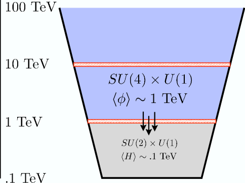
Figure 1: The energy scale and dependence of just a single stage of a Little Higgs theory. The tower of effective field theories (EFTs) begins with an $SU(4)\times U(1)$ EFT that spontaneously breaks at $1\ {\rm TeV}$, leaving behind an $SU(2)_{W}\times U(1)$ EFT which spontaneously breaks at $.1\ {\rm TeV}$.

Below 10 TeV the model is a linear-sigma model version of the $SU(4)\times U(1)_{X}$ Little Higgs [11]: At $f_{1}\sim 1\ {\rm TeV}$ a set of scalars, $\phi$, collectively and spontaneously breaks an $SU(4)\times U(1)_{X}$ gauge symmetry to the electroweak gauge group, $SU(2)_{W}\times U(1)_{Y}$. Two $SU(2)_{W}$ doublets, $H_{1}\ \&\ H_{2}$, are pNGB, and they remain in the low energy spectrum. These Higgs fields have tree-level interactions that promote $SU(2)_{W}\times U(1)_{Y}$ breaking to $U(1)_{{\rm E\&M}}$. We summarize the fields, scales, and symmetry structure in Figure 1.

The novelty of Little Higgs theories lies in the separation of scales. While $SU(4)\times U(1)_{X}$ breaks at $f_{1}\sim 1\ {\rm TeV}$, $SU(2)_{W}\times U(1)_{Y}$ breaks at a lower scale, $f_{0}\sim.1\ {\rm TeV}$. This hierarchy between $f_{1}$ and $f_{0}$ is enforced in the $SU(4)\times U(1)_{X}$ gauge theory by a set of global symmetries and their spurion structure. These approximate symmetries ensure cancellations of all quadratically divergent loop diagrams from renormalizable operators that might contribute to the masses of the $H_{1}\ \&\ H_{2}$ and destabilize the ratio $f_{0}/f_{1}$.

For just this section we impose a cutoff of $\Lambda=10\ {\rm TeV}$ on the theory. Without additional UV structure, naturalness would be lost if we allowed $\Lambda$ to be greater than $10\ {\rm TeV}$–although $H_{1}\ \&\ H_{2}$ are protected from quadratic divergences, the $\phi$ fields are not. In the non-linear sigma-models already present in the literature, [6]-[17], $10\ {\rm TeV}$ corresponds to the scale of strong-coupling due to the absence of the symmetry-breaking radial modes. By working in a linear-sigma model, we keep the theory at weak-coupling near $10\ {\rm TeV}$, which allows us to extend the theory perturbatively to $100\ {\rm TeV}$. In Section 3, we actually lift $\Lambda$ to $100\ {\rm TeV}$ and detail the perturbative UV structure that justifies our chosen spurion structure and maintains an insensitivity of the Higgs mass to high scales.

2.1 $SU(4)\times U(1)_{X}$ Breaking

The scalar sector of the $SU(4)\times U(1)_{X}$ gauge theory consists of fundamental fields, $\phi$, with the same $U(1)_{X}$ charge, $-1/4$. These $\phi$ fields are arranged in pairs, $\phi\ \&\ \phi^{\prime}$, with interactions designed to produce Goldstone bosons; we visually depict these interactions in Figure 2. This structure is familiar – if we replace $\phi\ \&\ \phi^{\prime}$ with $H_{1}\ \&\ H_{2}$ we find the usual scalar sector of a standard 2-Higgs-Doublet-Model (2HDM).

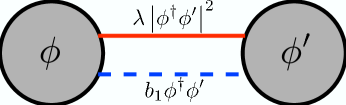
Figure 2:

As visual shorthand Figure 2 has two elements: shaded circles (which always represent fundamental scalar fields that have vev’s) and lines (which represent interactions between fields). Specifically, the diagram in Figure 2 represents the potential

$$V\supset-b_{1}\left(\phi^{\dagger}\phi^{\prime}+{\rm h.c.}\right)+m_{1}^{2}\left(\left|\phi\right|^{2}+\left|\phi^{\prime}\right|^{2}\right)+\lambda\left|\phi^{\dagger}\phi^{\prime}\right|^{2}.$$ (1)

For simplicity we’ve assumed that all the scalar masses in the theory are identical, though none of our results depend on this degeneracy. We also set all dimensionful operators to be of order $\sim 1\ {\rm TeV}$, the seemingly natural scale given a cutoff of $10\ {\rm TeV}$ (we discuss this assumption further in Section 2.3).

In the potential of Equation 1, the $b_{1}$-term promotes spontaneous symmetry breaking while the quartic $\lambda$ provides stability around the minimum. The potential has a global $U(4)$ symmetry, under which $\phi\ \&\ \phi^{\prime}$ are fundamentals. Due to this structure, $\phi\ \&\ \phi^{\prime}$ acquire vev’s $\sim 1\ {\rm TeV}$

$$\langle\phi\rangle=\left(\begin{array}[]{c}0\\ 0\\ 0\\ f_{1}\end{array}\right)\ \ \ \langle\phi^{\prime}\rangle=\left(\begin{array}[]{c}0\\ 0\\ 0\\ f_{1}\end{array}\right),{\ \rm with}\ f_{1}=\frac{b_{1}-m_{1}^{2}}{\lambda}.$$ (2)

The vev’s break the global $U(4)$ symmetry to $U(3)$ and produce 7 would-be Goldstone bosons. The would-be Goldstone bosons are eaten by the gauge bosons as the vev’s also break the gauge symmetry down to $SU(3)\times U(1)$.

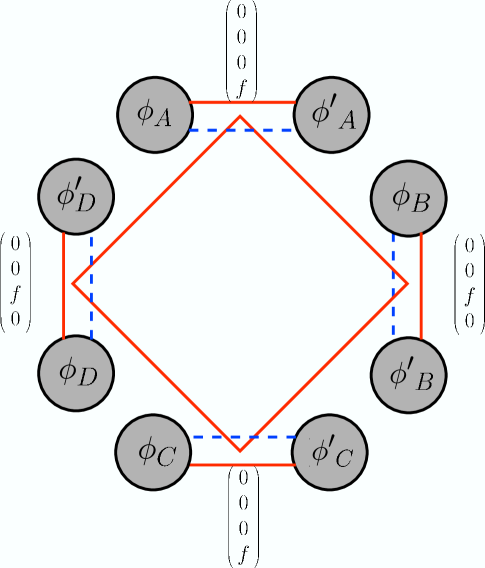
Figure 3: All 8 fields which contribute to the $SU(4)$ breaking. The visual shorthand is that of Figure 2 with one modification. The largest quartic links (those connecting two sets of pairs) have ends in the middle of each pair—which is shorthand for four separate quartics (equivalent to a red, solid line between each element of one pair and each element of the other pair). These specific quartic operators are described in Equation 3.

The full $SU(4)\times U(1)_{X}$ gauge theory contains four such pairs—each with the interactions described in Equation 1. Each of these pairs in isolation (no interactions between pairs, no gauge interactions) produces a set of 7 Goldstone bosons which includes one $SU(2)$ doublet, for a total of four Goldstone $SU(2)$ doublets. After we turn on interactions between pairs and gauge the $SU(4)$ symmetry, these four doublets divide into two groups: two of the four doublets are eaten by the $SU(4)/SU(2)_{W}$ gauge bosons; the remaining two are the pNGB we desire, $H_{1}\ \&\ H_{2}$. They have charges $(2,-1/2)$ under the remaining $SU(2)_{W}\times U(1)_{Y}$ EFT and are massless at tree-level.

We show the additional interactions between the pairs in Figure 3, where we arrange the pairs in a square whose edges represent quartic interactions between fields. With the labels of Figure 3 these additional quartic interactions are

$$V\supset\lambda\left(\left|\phi_{A}^{\dagger}\phi_{B}\right|^{2}+\left|{\phi^{\prime}}_{A}^{\dagger}\phi_{B}\right|^{2}+\left|\phi_{A}^{\dagger}\phi^{\prime}_{B}\right|^{2}+\left|{\phi^{\prime}}_{A}^{\dagger}\phi^{\prime}_{B}\right|^{2}\right).$$ (3)

Similar terms exist only for fields which are at neighboring vertices on the square, $(A,B)\rightarrow(B,C),(C,D)$ or $(D,A)$, for a total of sixteen new quartic interactions. The additional quartic interactions stabilize the $SU(4)\times U(1)_{X}\rightarrow SU(2)_{W}\times U(1)_{Y}$ breaking pattern by pushing the pairs of vev’s (at tree-level) into the structure indicated in Figure 3. The (mis)alignment of the vev’s which break $SU(4)$ can be guaranteed by the combination of the positive quartics between adjacent sites and the introduction of small $b$ terms and quartic couplings which stretches across the diamond to connect sites at opposite ends. A more detailed analysis of the remainder of the symmetry breaking structure is provided for reference in Appendix A.

Although each pair of fields of Figure 3 has a global $U(4)$ symmetry, the $SU(4)^{4}$ subgroup is explicitly broken to the diagonal $SU(4)$ by the extra quartic interactions between pairs. This diagonal $SU(4)$ is actually the gauged symmetry, and the gauge interactions also explicitly break the $SU(4)^{4}$ to the diagonal. With all interactions turned on, the global symmetry is reduced from $U(4)^{4}$ to $SU(4)\times U(1)^{4}$.

As shown in Ref. [11], after the $SU(4)\times U(1)_{X}$ symmetry breaks, the pNGB $H_{1}\ \&\ H_{2}$ are left with their own tree-level quartic interaction: $V\supset\lambda\left|H_{1}^{\dagger}H_{2}\right|^{2}$. Figure 4 shows the final Higgs structure. It is important to note that the generated quartic is the same size as the $SU(4)\times U(1)_{X}$ quartics of Equation 3. This quartic interaction is generated at tree-level after integrating out singlets with trilinear interactions and masses of order $f_{1}$.

We can generate the $b_{0}\sim.1\ {\rm TeV}$ term that’s required for $SU(2)_{W}\times U(1)_{Y}$ breaking by including seed terms, e.g. $b_{0}\phi_{A}^{\dagger}\phi_{B},\ldots$, in the original $\phi$ theory. These are the only terms that violate the $U(1)^{4}$ symmetry, so they are technically natural. Of the four would-be Goldstone electroweak singlets from the $U(1)^{4}_{\phi}$ breaking, two singlets are eaten by gauge bosons and the other two singlets pick up weak scale masses from the $b_{0}$ terms. The phenomenology of these singlets is described in Ref. [34], and otherwise the phenomenology is that described in [11]. For example, the ratio of Higgs vev’s (i.e., $\tan\beta$) goes like the inverse ratio of their diagonal masses. The top loop suppresses the “up-type” mass and therefore prefers large $\tan\beta$, which is good for keeping down the Yukawa coupling.

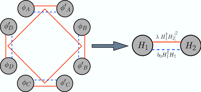
Figure 4: The full structure of symmetry breaking below $10\ {\rm TeV}$. The 8 fields of the $SU(4)$ Little Higgs theory spontaneously break and leave behind the indicated 2HDM.

2.2 Fermions & Yukawa Interactions

Fermions must also be embedded in representations of $SU(4)$, with $SU(4)\times U(1)_{X}$ gauge invariant Yukawa interactions. For example, the third generation quark doublet becomes a fundamental of $SU(4)$, with $\left(SU(3)_{c},SU(4),U(1)_{X}\right)$ quantum numbers $\left(3,4,5/12\right)$. We define $\hat{Q}_{3}=\left(Q_{3},T_{1},T_{2}\right)$ with $Q_{3}$ the third generation $SU(2)_{W}$ quark doublet. We write down a Yukawa interaction with

$$V\supset\left\{y_{TA}\phi_{A}^{\dagger}T^{c}_{A}+y_{TB}{\phi}_{B}^{\dagger}{T}^{c}_{B}+y_{TC}\phi_{C}^{\dagger}T^{c}_{C}\right\}\hat{Q}_{3},$$ (4)

where $T^{c}_{A},{T}^{c}_{B}\ \&\ T^{c}_{C}$ have quantum numbers $\left(\overline{3},1,-2/3\right)$. These interactions also preserve the global $SU(4)\times U(1)^{4}$ symmetry, just like the gauge and scalar interactions.

In the $SU(2)_{W}$ EFT below $\langle\phi\rangle$, the above Yukawa structure reproduces the SM fields and interactions. Consider the limit of degenerate $y_{T}$, with $y_{TA}=y_{TB}=y_{TC}$, which gives particularly simple results:

$$V \supset y_{t}H_{1}^{\dagger}Qt^{c}+m_{1}T_{1}T_{1}^{c}+m_{2}T_{2}T^{c}_{2},$$ (5)

with $y_{t}=y_{T}/\sqrt{2}$, $m_{1}=\sqrt{2}y_{T}f_{1},$ and $m_{2}=y_{T}f_{1}$. The diagonalized fields are $t^{c}=1/\sqrt{2}\left(T^{c}_{A}-T^{c}_{C}\right)$, $T_{1}^{c}=1/\sqrt{2}\left(T^{c}_{A}+T^{c}_{C}\right)$, and $T_{2}^{c}=T_{B}^{c}$. We discuss below the more general situation where the $y_{TX}$ (and $f_{1}$) differ.

We add a mass for the bottom quark with a non-renormalizable Yukawa interaction:

$$\frac{y_{B}}{\Lambda^{2}}\phi_{A}\phi_{B}{\phi}_{D}\hat{Q}_{3}b^{c},$$ (6)

where the $SU(4)$ indices are tied together with an antisymmetric 4-index epsilon tensor. After $SU(4)$ symmetry breaking, $H_{2}$ plays the role of the down-type Higgs, with Yukawa $y_{b}=y_{B}*f_{1}^{2}/\Lambda^{2}$, so $y_{B}\sim 1$. This operator preserves the global $SU(4)\times U(1)^{4}$ symmetry.

Anomaly cancellation occurs between the three generations [35, 29, 17]. The first two generation of quarks, $\hat{Q}_{1,2}$, are embedded as $\left(3,\overline{4},-1/12\right)$. Therefore, the down-type fermions have renormalizable interactions, while the up-type quarks have non-renormalizable interactions. The first two generations of down-type fermions have interactions like

$$V\supset\left\{y_{DB}{\phi^{\prime}}_{B}D^{c}_{B}+y_{DC}{\phi}_{C}{D}^{c}_{C}+y_{DD}{\phi^{\prime}}_{D}D^{c}_{D}\right\}\hat{Q_{1}},$$ (7)

where $D^{c}_{B},{D}^{c}_{C}\ \&\ D^{c}_{D}$ are $\left(\overline{3},1,1/3\right)$. The first two generations of up-type fermions get masses from the interactions

$$\frac{y_{U}}{\Lambda^{2}}\phi_{C}^{\dagger}{\phi^{\prime}}_{B}^{\dagger}{\phi}_{D}^{\dagger}\hat{Q}_{1}u^{c},$$ (8)

with $u^{c}=\left(\overline{3},1,-2/3\right)$.

For the first two generations, we are forced to choose non-degenerate Yukawa couplings. In fact, to ensure that the heavy lepton partners are heavy enough, we must take $y_{DC},y_{DD}\sim 1$, while $y_{D}$ has size similar to the relevant Yukawa coupling in the SM. This disparity in couplings leads to mixing between the light and heavy fermions after electroweak symmetry breaking. However, the effect of this mixing is minimized in the precision electroweak measurements when we begin to consider non-degenerate ratios of vev’s (e.g. $f_{A}/f_{C}\sim 3-5$) [11, 21].

All three generations of leptons are embedded as $(1,4,-1/4)$. For each generation, three ($SU(4)\ {\rm and}\ U(1)$) singlet fields $N$ field with charges $\left(1,1,0\right)$ are used (analogous to the $D^{c}$ and $T^{c}$ above), while one $e^{c}$ field with charges $\left(1,1,-1\right)$ is introduced to give the electron a mass (analogous to the $u^{c}$ and $b^{c}$ above).

2.3 Loop Corrections

Although $H_{1}\ \&\ H_{2}$ remain massless at tree-level, no unbroken symmetry prevents masses from being generated at loop level. The Higgs sector is massless in the limit of the exact unbroken $U(4)^{4}$ symmetry, but we have dimensionless ${\cal O}(1)$ spurions ($g,y_{T},\lambda$) which explicitly break the global symmetry to $SU(4)\times U(1)^{4}$. We estimate the size of the Higgs masses, and the naturalness of the theory, by calculating the size of the loop contributions to operators that we’ve ignored in the theory—assuming that physics above the cutoff contributes corrections of the same magnitude.

We find that these loops are parametrically under control, since the unbroken global $U(1)$ symmetries prevent dangerous dimension-two operators which could be proportional to the renormalizable ${\cal O}(1)$ spurions and powers of the cutoff, $\Lambda$—at every loop order. The largest corrections to the Higgs mass are from logarithmically divergent operators, which always yield corrections to Higgs masses that are proportional to $f_{1}^{2}/(4\pi)^{2}$ only.

We focus on operators generated in the full, unbroken $SU(4)\times U(1)_{X}$ gauge theory from the renormalizable interactions. The operators generated in the unbroken $SU(4)\times U(1)_{X}$ break into four representative types described below. (The notation is $M,N\in\left\{A,B,C,D\right\}$ and $\phi_{M}$ can refer to either $\phi_{M}$ or ${\phi^{\prime}}_{M}$.)

• $\phi^{\dagger}_{M}\phi_{M}$

These dimension-two operators (e.g. $\phi^{\dagger}_{A}\phi_{A}$ or ${\phi^{\prime}}^{\dagger}_{A}{\phi}_{A}$) are already present in the theory as mass terms for the $\phi$ fields. No masses for $H_{1}\ \&\ H_{2}$ are generated by these terms, since both preserve the largest global symmetry, $U(4)^{4}$, under which $H_{1}\ \&\ H_{2}$ are Goldstone bosons. Nevertheless, $\phi^{\dagger}_{A}\phi_{A}$ can be produced by quadratically divergent gauge, scalar, and fermion loops which set the naturalness scale for the mass of the $\phi$ fields and the breaking scale $f_{1}$. The contributions are listed in Appendix B, and give

$$m^{2}_{\phi}\stackrel{{\scriptstyle<}}{{{}_{\sim}}}10\left(\frac{\Lambda}{4\pi}\right)^{2}.$$ (9)

The largest contribution comes from the $\sqrt{2}$ enhanced top Yukawa ($y_{T}(1\ {\rm TeV})\sim 1.25$), while gauge and scalar loops contribute about a $1/3$ as much.

• $\phi^{\dagger}_{M}\phi_{N}$

These dimension-two operators (e.g. $\phi^{\dagger}_{A}\phi_{B}$) will generate masses for $H_{1}\ \&\ H_{2}$, since they break the $SU(4)^{4}$ global symmetries. However, $\phi^{\dagger}_{A}\phi_{B}$ violates the unbroken $U(1)_{A}$ and $U(1)_{B}$ symmetry, so it can only be proportional to those spurions which also violate $U(1)_{A}$ and $U(1)_{B}$, or is the spurion of this symmetry violation. Setting $b_{0}$ at $\sim.1\ {\rm TeV}$, these operators are safely ignored. Note that as long as all of the dimensionless ${\cal O}(1)$ spurions preserve the $U(1)^{4}$ symmetry, they cannot generate $\sim\Lambda^{2}$ contributions to these operators.

We could also consider operators of the form $\left(\phi_{M}^{\dagger}\phi_{N}\right)\left(\phi_{P}^{\dagger}\phi_{P}\right)$ which also break the $U(1)$ global symmetries. These will be generated by finite loops involving $\phi^{\dagger}_{M}\phi_{N}$ and are naturally small.

• $\left(\phi_{M}^{\dagger}\phi_{M}\right)\left(\phi_{N}^{\dagger}\phi_{N}\right)$

These dimension-four operators (e.g. $\left(\phi_{A}^{\dagger}\phi_{A}\right)\left(\phi_{B}^{\dagger}\phi_{B}\right)$) preserve the global $U(4)^{4}$ symmetry, so do not lead to masses for $H_{1}\ \&\ H_{2}$.

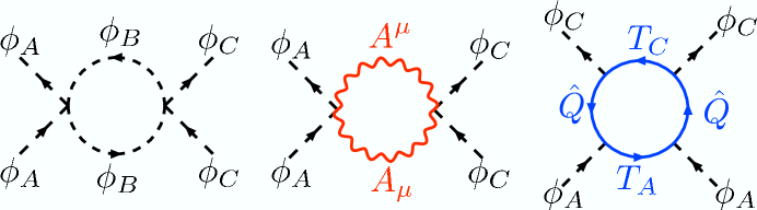
Figure 5: The three types of loops (scalar, gauge, and fermion loops, respectively) that lead to logarithmically divergent dimension-four operators. These operators contribute corrections to the masses of the pseudo-Goldstone bosons of order $f_{1}^{2}/16\pi^{2}$.

• $\left(\phi_{M}^{\dagger}\phi_{N}\right)\left(\phi_{N}^{\dagger}\phi_{M}\right)$

Consider the operator $\left(\phi_{A}^{\dagger}\phi_{C}\right)\left(\phi^{\dagger}_{C}\phi_{A}\right)$. This dimension-four operator preserves the $U(1)_{A}\ \&\ U(1)_{C}$ symmetries, so it can be generated by the ${\cal O}(1)$ spurions ($g,y_{T},\lambda$). It also violates the $SU(4)^{4}$ symmetry, so it is relevant for producing a mass for $H_{1}$. However, contributions to this operator are only logarithmically divergent (the coupling is dimensionless), and do not yield quadratic sensitivity to $\Lambda$. The diagrams that generate these operators at one loop are shown in Figure 5. These are the most divergent renormalizable operators one can write down that preserve the $U(1)^{4}$ symmetries and generate masses for the low-energy Higgs sector.

After expanding the fields in terms of their Higgs components, we find that the typical dimension-four operator predicts

$$\frac{\kappa}{8\pi^{2}}\left|\phi_{A}^{\dagger}\phi_{C}\right|^{2}\rightarrow m^{2}_{H_{1}}\sim\kappa\left(\frac{f_{1}}{4\pi}\right)^{2}.$$ (10)

Operators with $A\rightarrow\{A,A^{\prime}\}$ and $C\rightarrow\{C,C^{\prime}\}$ (four operators in total) can also give contributions to $m^{2}_{H_{1}}$ of the same size, while operators with $A\rightarrow\{B,B^{\prime}\}$ and $C\rightarrow\{D,D^{\prime}\}$ contribute to $m^{2}_{H_{2}}$.

We estimate the size of the loop contributions to these operators by computing the logarithmically divergent piece of the effective potential, with couplings constants evaluated at $1\ {\rm TeV}$ using the RGE’s given in Appendix C. The largest contributions at this stage are from scalar and fermion loops, while gauge loops are smaller due to the small gauge couplings.

The number of scalars which contribute to the loops shown in Figure 5 is determined by the number of indirect links between the $\phi_{A}$ and $\phi_{C}$. For this stage, there are four such links (one each through $\phi_{B},\phi^{\prime}_{B},\phi_{D},\ \&\ \phi^{\prime}_{D}$), which gives a factor of $4^{1}$,

$$\kappa_{s}=\left(\ln{10}\right)\ 4^{1}\lambda^{2}\rightarrow m^{2}_{H}\sim 9\left(\frac{f_{1}}{4\pi}\right)^{2}.$$ (11)

In the estimate for $m_{H}^{2}$ we have included the contribution from all four operators (those with $A\rightarrow A^{\prime}$ and/or $C\rightarrow C^{\prime}$) and used the running value of $\lambda(1\ {\rm TeV})\sim.5$, assuming a low energy value $\lambda(.1\ {\rm TeV})\sim.5$. It is important to note that the fine-tuning for this (and all) stages is associated with the Higgs mass squared $=\lambda v$ where $v$ is the electroweak vev.

Fermions give a contribution which scales with $N_{c}$,

$$\kappa_{f}\sim 2N_{c}y_{TA}^{2}y_{TC}^{2}\ln{10}\rightarrow m^{2}_{H}\sim 33\left(\frac{f_{1}}{4\pi}\right)^{2}.$$ (12)

Again, we have included the contribution from all induced operators in the estimate for $m^{2}_{H}$ and used the running value of the top Yukawa $y_{T}(1\ {\rm TeV})\sim 1.25$. The top Yukawa is larger than 1 due to the $\sqrt{2}$ normalization factor described below Equation 5. These corrections are larger than those present in the non-linear sigma models because of the enhancement of the top Yukawa and the presence of non pNGB scalar fields. This is worse than the minimal linear sigma model completion of the $SU(4)$ little Higgs theory because our completion has two scalars in the fundamental representation for each vev in the non-linear sigma model (e.g. fields $A$ and $A^{\prime}$). The doubling is in anticipation of the tower: the little Higgs stages produce two Higgs doublet models in the IR, so the linear sigma models which produce the symmetry breaking should also be “two-scalar fundamental models”, in analogy with two-Higgs doublet models.

3 Below 100  TeV

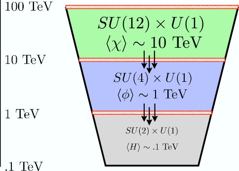
Figure 6: The energy scale and structure of a two-stage Little Higgs theory. As in Figure 1, the theory can be represented by successive stages of EFT’s: A spontaneously broken $SU(12)\times U(1)$ gauge theory lives between $10\ \&\ 100\ {\rm TeV}$, leaving behind a spontaneously broken $SU(4)\times U(1)$ gauge theory that lives between $1\ \&\ 10\ {\rm TeV}$, which leaves behind a spontaneously broken $SU(2)\times U(1)$ gauge theory that lives between $.1\ \&\ 1\ {\rm TeV}$.

As promised we now try to lift the cutoff to $100\ {\rm TeV}$, but we meet with immediate obstacles. Absent new interactions, fine-tuning first creeps in through the mass of the $\phi$ fields; Unlike the electroweak scale, the scale of $SU(4)$-breaking is sensitive to quadratic divergences proportional to the cutoff which generate the operators $\phi^{\dagger}_{M}\phi_{M}$. Even though the electroweak scale, $f_{0}$, remains insensitive to quadratic divergences, $f_{0}$ retains sensitivity to $f_{1}$. As $\Lambda$ is pushed to $100\ {\rm TeV}$, fine-tuning is introduced into the weak-scale.

Therefore, to push the cutoff, $\Lambda$, up to $100\ {\rm TeV}$ requires introducing new interactions if the theory is to remain natural. These new interactions should remove quadratic divergences to the $SU(4)$ breaking scale, $f_{1}$, without reintroducing unnatural scale dependence into the electroweak breaking scale, $f_{0}$.

We attempt to satisfy this stringent requirement by embedding the $SU(4)\times U(1)_{X}$ gauge theory into an $SU(12)\times U(1)_{Z}$ gauge theory. This gauge theory is cutoff by the scale $\Lambda\sim 100\ {\rm TeV}$, and interactions are such that the $SU(12)\times U(1)_{Z}$ gauge theory is collectively and spontaneously broken at the scale $f_{2}\sim 10\ {\rm TeV}$ by a set of fundamental scalars, $\chi$. The $SU(4)\times U(1)_{X}$ gauge theory of Section 2 is left over, with the fields $\phi$ surviving as light pseudo-Goldstone bosons without quadratic sensitivity to $\Lambda\sim 100\ {\rm TeV}$. All required $SU(4)$ quartics – both those that directly stabilize $\phi$ vev’s and those that will eventually stabilize the Higgs vev – are again generated at tree-level. All other quartic interactions (which we assumed were absent in the $SU(4)$ theory) are generated at 1-loop order and are suppressed. However, the suppression is not quite large enough, due to the compensating factor of the number of fields, and some fine-tuning remains at this stage. We review the fields and scales involved in Figure 6.

3.1 $SU(12)\times U(1)_{Z}$ Breaking

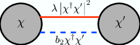
Figure 7:

We build the $SU(12)\times U(1)_{Z}$ sector up iteratively from the $SU(4)\times U(1)_{X}$ theory. The basis of this pattern is again the unit shown in 7 which now visually depicts two fundamental scalars $\chi\ \&\ \chi^{\prime}$ of the $SU(12)$ gauge theory and their interactions, and we have set $b_{2}\sim 10\ {\rm TeV}$. We proceed to build up a pattern of squares based on this unit, such that once spontaneous symmetry breaking occurs in the $SU(12)$ theory, we are left with the pattern of Figure 3 in the (low energy EFT) $SU(4)$ gauge theory below $10\ {\rm TeV}$.

A single pair of $\chi$ fields produces a set of $U(12)/U(11)$ would-be Goldstone bosons along the flat directions of the $\chi$ potential. These would-be Goldstone bosons are actually eaten by the gauge bosons, as the gauge symmetry is broken down to $SU(11)\times U(1)$.

A single square of $\chi$ fields (four pairs, with scalar interactions just like those of Figure 3 with $\phi\rightarrow\chi$) leaves a pair of pNGB, $\phi$. The counting is identical to that of Section 2: each square of $\chi$ fields breaks the rank of the gauge group by 2; each square produces 2 would-be Goldstone fundamentals of $SU(4)$ that are eaten by the $SU(12)$ gauge bosons; each square produces another 2 pNGB fundamentals of $SU(4)$ that remain light and become a pair of $\phi$ fields in the $SU(4)$ EFT.

The full $SU(12)\times U(1)_{Z}$ gauge theory contains 4 such squares, to generate the 8 light pNGB scalars, $\phi$ in the $SU(4)\times U(1)_{X}$ theory. We require additional quartic interactions between squares as indicated in Figure 8. These quartic links make it more energetically favorable for the vev’s in each square to separate and break the gauge symmetry to $SU(4)$, not $SU(10)$. The net result is that the fields $\chi$ occur in sets of four (these are the two pairs on opposite corners of a smaller square) with vev’s in the same position. Each set of four has a vev in a unique position, which breaks the gauge group from $SU(12)\times U(1)_{Z}$ to $SU(4)\times U(1)_{X}$ and produces the 8 pNGB, $\phi$. The alignment of vev’s within the small squares is guaranteed as in Section 2, by the positive quartics and the introduction of small $b$ terms and quartics across the small square. The (mis) alignment of vev’s between fields across the largest square can be guaranteed by the outer positive quartics and the even smaller $b$ terms and quartics introduced across the largest square to ensure subsequent alignment in the $SU(4)$ theory.

Together, the quartic links collapse to produce the quartic interactions as shown in Figure 8. As the vertices of each small square collapse to become a pair of $\phi$ fields, the edges collapse to become the quartic interaction for the pair. The largest square of links collapses to become the square of links in the $SU(4)$ gauge theory that leads to $SU(4)$ quartics and the final quartic in the $SU(2)_{W}$ 2HDM. The mechanism that accomplishes this is identical to that of Section 2–and occurs at tree-level. The low-energy quartics all have the same value as the original $SU(12)\times U(1)_{X}$ quartics and come from integrating out scalars with trilinear interactions and masses of order $f_{2}$.

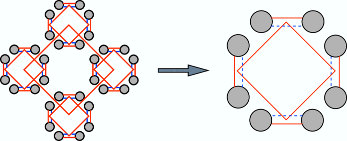
Figure 8: The $SU(12)$ gauge theory (left) juxtaposed with the $SU(4)$ gauge theory (right). Every pair of fields in the $SU(4)$ theory is replaced with a square of 8 fields in the $SU(12)$ theory. Shaded circles are again fields that get vev’s, while red, solid lines represent $U(1)$ preserving quartic interactions between fields at opposite ends of the line, and the blue dashed lines represent $U(1)$ breaking dimension-two operators ($b$-terms) between fields at opposite ends of the line.

The $b_{1}$ and $b_{0}$-terms that promote $SU(4)$ and $SU(2)_{W}$ breaking, respectively, are added in by hand by linking the relevant $\chi$ fields. Such links are again technically natural in the larger theory. All singlets that are would-be Goldstones of the spontaneously broken $U(1)_{\chi}$ global symmetries are eaten by $SU(12)\times U(1)_{Z}$ gauge bosons or pick up $\sim f_{1}$ masses from the explicit symmetry breaking terms $b_{1}$.

The theory begins with a large $SU(12)\times U(1)^{16}$ global symmetry that is preserved by gauge, scalar, and Yukawa interactions. When the $\chi$ fields acquire vev’s, this symmetry is broken to $SU(4)\times U(1)^{8}$, which is further broken to $SU(4)\times U(1)^{4}$ by the $b_{1}$ interactions. This is exactly the global symmetry we used to show the absence of all dangerous dimension two operators in the $\phi$ theory below $10\ {\rm TeV}$.

3.2 $U(1)_{Z}$ & Fermions

All scalars $\chi$ have charge $Z_{\chi}=-1/12$ under $U(1)_{Z}$, and the $U(1)_{Z}$ mixes with one of the diagonal generators of $SU(12)$ to produce $U(1)_{Z}$.

Specifically:

$$U(1)_{X}=-\frac{1}{12}{\rm diag}\{2,2,2,2,-1,-1,-1,-1,-1,-1,-1,-1\}+U(1)_{Z}$$ (13)

for a fundamental of $SU(12)$. We note that

$$g_{X}=\frac{gg_{Z}}{\sqrt{g^{2}+\frac{g_{Z}^{2}}{3}}}.$$ (14)

We embed fermions as described in Section 2: the third generation has interactions that remove quadratic divergences from the top sector only (with third generation fermion charges $W_{{\tilde{Q}}_{3}}=7/12$), while the first two generations remove divergences from the down-type quarks and neutrinos ($W_{{\tilde{Q}}_{1,2}}=-3/12$, $W_{\tilde{L}}=-1/12$).

In Section 2.2, we used a set of Yukawa interactions that caused the Yukawa couplings to be enhanced by a factor of $\sqrt{2}$ in the $SU(4)\times U(1)_{X}$ stage. To keep the Yukawa interactions under control in the $SU(12)$ theory, we write down an interaction of the form $\left(y\chi+{y^{\prime}}{\chi^{\prime}}\right)\tilde{T}\tilde{Q}$ instead of the single interaction $y\chi\tilde{T}\tilde{Q}$. This embedding causes a reduction in the value of the $SU(12)$ Yukawa by a factor of $\sqrt{2}$, and brings the top Yukawa under perturbative control. However, the $U(1)_{\chi}$ and $U(1)_{\chi^{\prime}}$ symmetries which are only broken by $b_{2}\sim 10\ {\rm TeV}$ terms are now also broken by dimensionless combinations of $y$ and $y^{\prime}$. This has the advantage of generating the $b_{2}$ term naturally, but makes it difficult to write down simple UV completions of the fermion sector that will not introduce dangerous scale dependence. We therefore only use this embedding in the $SU(12)$ stage.

This embedding is again anomaly free. The non-renormalizable interactions needed for the bottom quark now involve 11 $\chi$ fields and have overall coefficient, $y_{B}/f_{2}^{10}$. Since the mass suppression is $f_{2}$ and not $\Lambda$, the bottom Yukawa forces us to a strong-coupling limit at the cutoff that we address in Section 3.4. To add another stage would require a new embedding for both the top and bottom quarks.

3.3 Loop Corrections

After the $SU(12)$ symmetry breaking, the $\phi$ fields remain massless at tree-level (up to small $b$ terms), but we must again consider masses that might be generated at loop level. The global $U(1)_{\chi}$ symmetries again prevent the most dangerous dimension two-operators which could give $\sim\Lambda^{2}$ masses to the $\phi$ fields from the renormalizable ${\cal O}(1)$ spurions at all loop orders. Here we focus on the form of corrections from just the renormalizable sector.

The largest corrections to the $\phi$ masses come from logarithmically divergent operators that give masses proportional only to $f_{2}^{2}$. The $U(1)$ symmetry structure also prevents dangerous contributions to the Higgs masses: No masses are generated which are proportional to the ${\cal O}(1)$ spurions times powers of $\Lambda^{2}$ or $f_{2}^{2}$, again at all loop orders.

The types of operators that we’ve ignored in the full $SU(12)\times U(1)_{X}$ theory are ($J,K$ run over all 32 $\chi$ fields)

• $\chi^{\dagger}_{J}\chi_{J}$

These dimension-two operators are already present in the theory as mass terms for the $\chi$ fields. No masses for $\phi$ are generated by these terms, since $\chi_{J}^{\dagger}\chi_{J}$ preserves the largest global symmetry, $U(12)^{16}$, under which the $\phi$ fields (and therefore, the Higgs fields) are exact Goldstone bosons. Nevertheless, these operators are generated by quadratically divergent gauge, scalar, and fermion loops and set the naturalness scale for the mass of the $\chi$ fields and the breaking scale $f_{2}$. The contributions are listed in Appendix B, and give

$$m^{2}_{\chi}\stackrel{{\scriptstyle<}}{{{}_{\sim}}}7\left(\frac{\Lambda}{4\pi}\right)^{2},$$ (15)

The contribution grows with the number of scalar fields and the size of the weak gauge group, but is offset by the running coupling constants ($g_{w}(10\ {\rm TeV})\sim.6,\lambda(10\ {\rm TeV})\sim.3$), now assuming a low energy value of $\lambda\sim.7$. The fermion contribution is reduced compared to that in the $SU(4)\times U(1)_{X}$ theory because of the reduction in the Yukawa couplings from the doubling of interactions, so $y_{T}(10\ {\rm TeV})\sim.9$. In this stage, the $b_{1}$ terms are also generated with the same size by the enhanced fermion structure that mixes the primed and unprimed fields.

• $\chi^{\dagger}_{J}\chi_{K}$

These dimension-two operators will generate masses for both the $\phi$ sector and the Higgs sector, since they break the $SU(12)^{12}$ global symmetries. However, these operators violate the unbroken $U(1)^{16}$ symmetries, so they must be proportional to those spurions which also violate the relevant $U(1)$ symmetries. The only coefficients which violate these symmetries are the $b_{1}$ terms (which can only generate masses for the $\phi$ fields proportional to $b_{1}$), and the $b_{0}$ terms (which can generate masses for the $\phi$ fields and the Higgs fields). Both sets of $b$ terms give corrections that are under control. As in the $SU(4)$ stage, operators of the form $\left(\chi_{J}^{\dagger}\chi_{K}\right)\left(\chi_{L}^{\dagger}\chi_{L}\right)$ will be generate by finite loops and will be small (i.e., have a negligible effect on the $\phi$ masses).

• $\left(\chi_{J}^{\dagger}\chi_{J}\right)\left(\chi_{K}^{\dagger}\chi_{K}\right)$

These dimension-four operators preserve the global $U(12)^{16}$ symmetry under which the $\phi$ (and Higgs) fields are exact Goldstone bosons, so no mass terms are generated by these operators.

• $\left(\chi_{J}^{\dagger}\chi_{K}\right)\left(\chi_{K}^{\dagger}\chi_{J}\right)$

These dimension-four operators preserve the $U(1)^{16}$ global symmetries, so they are generated by the ${\cal O}(1)$ spurions ($g,y_{T},\lambda$). The operators also violate the $U(12)^{16}$ symmetries, so they are relevant for producing a mass for $\phi$ proportional to $f_{2}^{2}$ after the vev’s for $\chi$ are plugged in. Operators which gives $f_{2}^{2}$ masses to the $\phi$ fields are quartic interactions between $\chi$ fields which have vev’s in the same position.

These operators are only logarithmically divergent, and do not yield quadratic sensitivity to $\Lambda$. The diagrams that generate these operators are identical to those shown in Figure 5, except now involving $\chi$ fields and the $SU(12)$ gauge bosons and quark fields. These are the only renormalizable operators one can write down that preserve the $U(1)^{16}$ symmetries and generate masses for the low-energy $\phi$ sector.

None of these operators, however, generate $f_{2}^{2}$ masses for the Higgs sector. This can be seen in two ways: if one carefully expands the $\chi$ fields in terms of the Higgs fields, it can be seen that the $\chi$ vev’s never generate a Higgs mass term; or if one notes that the EFT below the $\chi$ vev’s contains an unbroken $U(1)^{4}$ symmetry on the $\phi$ fields that prevents all dimension two operators that lead to Higgs masses proportional to $f_{2}$. These are the same $U(1)$ symmetries we used to explain the absence of large $\phi^{\dagger}_{M}\phi_{N}$ terms in Section 2.3.

After expanding the fields in terms of their Higgs components, we find that the typical dimension-four operator predicts

$$\frac{\kappa}{8\pi^{2}}\left|\chi_{J}^{\dagger}\chi_{K}\right|^{2}\rightarrow m^{2}_{\phi}\sim\kappa\left(\frac{f_{2}}{4\pi}\right)^{2}.$$ (16)

For each field $\phi_{M}$, there can be four operators which contribute to its mass.

The number of scalars which contribute to the loops shown in Figure 5 is determined this time by the number of indirect links between the $\chi$ fields. For this stage, there are 20 such links (four from within the little square, and 8 each from the neighboring squares):

$$\kappa_{s}=\left(\ln{10}\right)\ \left(4^{1}+4^{2}\right)\lambda^{2}\rightarrow m^{2}_{\phi}\sim 15\left(\frac{f_{2}}{4\pi}\right)^{2}.$$ (17)

In the estimate for $m_{\phi}^{2}$ we have the contribution from all four operators and used the running value of $\lambda(10\ {\rm TeV})\sim.3$, assuming a low energy value $\lambda(.1\ {\rm TeV})\sim.7$. The quartic coupling is running weak due to contributions from the top and gauge sectors. Gauge loops contribute corrections that are a bit smaller in size, while fermion contributions are larger

$$\kappa_{f}\sim 2N_{c}y^{4}\ln{10}\rightarrow m^{2}_{\phi}\sim 36\left(\frac{f_{2}}{4\pi}\right)^{2}.$$ (18)

Again, we have included the contribution from the four separate operators that can contribute in the estimate for $m^{2}_{\phi}$, and used the running $y_{T}(10\ {\rm TeV})\sim.9$. We have not included other potential contributions from the other couplings added previously to reduce the couplings from $\sim\sqrt{2}$ to $\sim 1$, and thus this estimate may be low. While all of these logarithmically divergent terms give the right parametric dependence, fine-tuning is introduced by typically neglected numerical prefactors: the number of scalar fields, rank of the gauge group, and combinations of $N_{c}$ and the large Yukawa couplings.

The operators just described lead to masses for the $\phi$ fields of order $f_{2}$, but there are also operators (produced in the $SU(12)$ theory) that can contribute to $Higgs$ masses of order $f_{1}$ when the $SU(4)$ gauge theory breaks. Such operators are quartics that mix a field from one square, from any other field on the diametrically opposed square. These operators do not give $\sim f_{2}$ masses to the Higgs since the vev’s of these two fields miss (because of the preserved $U(1)_{\phi}$ symmetries), but they do lead to operators like $\left|\phi^{\dagger}_{A}\phi_{C}\right|^{2}$ that we considered at the end of Section 2.3.

We assumed these operators were absent at tree-level in the $SU(4)$ theory of Section 2 and must show that the $SU(12)$ UV completion does not generate them with large coefficients. These dimension-4 operators are generated at 1-loop order by logarithmically divergent diagrams. The largest of these comes from Yukawa interactions, and the coefficients generated have size $\sim.1$, while contributions from scalar operators are of order $.04$. These quartics are $10-30\%$ perturbations compared to the tree level quartics and are of the same size as the corrections calculated at the end of Section 2.3.

3.4 A Non-Linear Sigma Model

The non-renormalizable bottom Yukawa (requiring an epsilon tensor and 11 $\chi$ fields) is a dimension-14 operator which would produce way too small of a bottom quark mass unless the theory was strongly coupled at $\Lambda$. Thus, we are forced into the non-linear sigma model where the radial modes including in the $\chi$ fields are pushed to the cutoff. In this case, we keep the same interactions as before, except now each $\chi$ field is a dimensionless non-linear sigma model field (see [11] for the analogous discussion in the $SU(4)\times U(1)$ model). The coefficient of the non-renormalizable bottom interaction is $\sim 1$ times the appropriate powers of $f_{2}$ in order to produce the correct standard model Yukawa coupling.

The non-linear sigma model has the significant advantage of removing $1/2$ of the scalar fields since only one $\chi$ field is needed to describe each pNGB $\phi$ field (instead of the two fields $\chi,\chi^{\prime}$. This reduces the effect of the logarithmic divergences by 1/2, so the NDA estimate for the fine-tuning is similarly reduced.

4 Dreams of a Goldstone Tower

Up to this point we have described a two-stage Little Higgs model with a cutoff of $100\ {\rm TeV}$. We have successfully removed all dangerous loop contributions – there are no quadratic divergent contributions to the Higgs mass and all log-divergent and finite contributions are proportional to only the lowest breaking scale $f_{1}$. At the same time, large numerical factors render the “safe” loop contributions unpalatable by reintroducing fine tuning. The existence of these large numbers is due in part to the large coupling times color factor in the top sector and due in part to the geometric increase in the number of fields. In spite of this drawback, the natural repeatability of the structure of our theory compels us to explore the possibility of a full tower of symmetry breaking. We find a toy model of a tower with reduced fine-tuning and indications of how one might remove the tuning completely.

The stacking of little Higgs modules is quite easy. Every two-scalar-fundamental sector of the theory is completed by eight fundamentals of the larger gauge group, as the original two-Higgs-doublet model of $SU(2)\times U(1)$ completes into an $SU(4)\times U(1)$ gauge theory with eight fundamentals. At each stage the number of scalars in the fundamental representation increases by a factor of four, i.e.,

$$N_{s}=2\times 4^{k},$$ (19)

where $k$ labels the stage of breaking, $f_{k}$: $f_{0}=100\ {\rm GeV}$, $f_{1}=1\ {\rm TeV}$, $f_{k}=10^{k-1}\ {\rm TeV}$. Each one of the groups of eight fundamentals which produces a two-scalar-fundamental model breaks the rank of the gauge group by 2. Thus, the rank of the group in the upper stage is equal to the rank of the group in the stage just below it plus the number of fundamental scalars. For example, $SU(2)$ with 2 little Higgses required an $SU(2+2)$ theory with 8 fundamentals above it, which required an $SU(4+8)$ theory with 32 fundamentals above that, etc. (see Table 1). This counting also makes it clear that at every stage, there are exact (up to $b$ terms) $U(1)_{scalar}$ symmetries which rotate by a phase each of the $SU(N)$ fundamentals. Each $U(1)_{scalar}$ at one stage is a linear combination of a broken diagonal generator of the gauge group in the upper stage and the $U(1)_{scalar}$ symmetry that rotates the phase of the linear combination of scalars responsible for the breaking in the upper stage.

Breaking Scale	$N_{W}$	$N_{S}$	cutoff
$f_{0}\sim.1\ {\rm TeV}$	2	2	$1\ {\rm TeV}$
$f_{1}\sim\ {\rm TeV}$	4	8	$10\ {\rm TeV}$
$f_{2}\sim 10\ {\rm TeV}$	12	32	$100\ {\rm TeV}$
$f_{k}\sim 10^{k-1}\ {\rm TeV}$	$2+\frac{2}{3}\left(4^{k}-1\right)$	$2\cdot 4^{k}$	$10^{k}\ {\rm TeV}$

Table 1:

What is clear from this discussion (and the table) is that this theory quickly becomes a large $N$ theory (with $N_{s}\sim N$). This could in principle be okay if everything has the right $N$-scaling behavior to keep the theory perturbative and functional. In practice, this means gauge couplings squared $g^{2}$, Yukawa couplings squared $y^{2}$, and quartic couplings $\lambda$ must all scale like $1/N$. Then one should analyzing the running and matching of the ’t Hooft coupling, e.g., $g^{2}N$, to see if it remains perturbative in the UV. Amazingly enough, in the simplest version of the field content (only $SU(N)$ gauge bosons and scalars), the average ’t Hooft coupling approaches an asymptotic value that is perturbative! See Figure 9.

Figure 9: Evolution of the ’t Hooft coupling, $g^{2}N_{w}/(4\pi)$ from the one renormalization group equations. The discontinuities are caused by the changing value of $N_{w}$ at every decade of energy.

However, there are some operators/couplings which do not obey the necessary scaling to preserve the structure. The most obvious ones are the hypercharge and $SU(3)$ color couplings which, while obtaining beta functions which scale linearly with $N$, are asymptotically unfree and therefore hit a Landau pole at some intermediate scale (though they remain perturbative at 100 TeV). Some level of unification of gauge groups would be required to avoid these problem in a model like ours. A more immediate problem is the bottom Yukawa coupling (among others) which already become impossible to write down if the $SU(12)$ model below 100 TeV is a linear sigma model (what would be required to continue the tower). In the linear sigma model, the bottom Yukawa requires an operator of dimension 14! However, in order for Yukawas to follow true $1/N$ scaling, some fermions must appear in representations with two indices - i.e., those which have a Dynkin index which goes like $N$. Unfortunately, this doesn’t change the situation for fermions like the bottom due to the requirement of the epsilon tensor and thus remains a stopping point for realistic towers in this class of models.

The above issue we regard as peripheral to the central point of discovering a perturbative theory with order one couplings in the infrared in which naturally light scalars appear. If we shed things like hypercharge and Yukawa couplings and focus on the structure of the scalar-gauge theory we find indications that a full tower may be possible. For example, at every stage there is a cutoff $\Lambda$ and a mass term for the scalar fields $m^{2}|\phi|^{2}$ whose value is generated by a one loop quadratic divergence $m^{2}\sim g^{2}N\Lambda^{2}/16\pi^{2}$. If $g^{2}N\sim 1$ then our one loop suppression remains and $m\sim\Lambda/4\pi$. The vev of $\phi$, $f_{k}$, however should be (without fine tuning) $f_{k}\sim\sqrt{m^{2}/\lambda}\sim\sqrt{N}\Lambda/4\pi$! One might worry that such a vev would be out of the range of validity. One hint that it may not be is that because all couplings of $\phi$ are of order $1/\sqrt{N}$, then this vev only generates masses for other fields (e.g., gauge bosons) below the cutoff. The renormalizable operators exhibit an approximate shift symmetry for $\phi$ only broken by effects suppressed by powers of $N$. Treating these as spurions, the higher dimensional operators contributing to the potential would be functions of $\phi/(\sqrt{N}\Lambda)$ times loop factors at weak coupling. Under these conditions, the validity of the effective theory is maintained.

The real sticking point comes from the renormalization group flow of the quartic operators detailed in Appendix C. While there is a range of quartic and $g^{2}$ values for which the quartic’s beta function is negative, it is not a stable range - in other words, the couplings flow away from these values at eventually the quartics become IR free and stop tracking the $g^{2}$ coupling. This appears to be a problem with the actual coefficients in the beta functions and thus the stack may still be possible with some other quartic structure or gauge structure involving different representations. This is a possibility we will continue to pursue. We are not, however, far off. As it stands, the quartics in our model track effectively for a cutoff $\Lambda\stackrel{{\scriptstyle<}}{{{}_{\sim}}}10^{5}\ {\rm TeV}$. In addition, the so-called “bad” quartics at each stage run in such a way as to stay a loop factor below the “good” quartics, as long as they start that way at the high scale. This is the sign that in the large-$N$ theory, large logs do not become an issue.

The other sticking point is the fact that high scales, $g^{2}N/4\pi\equiv\alpha_{\rm{}^{\prime}tHooft}$ is not $\sim 1/4\pi$ but $\sim 1$. While this is still semi-perturbative, it would naturally allow (without any fine tuning) only a factor of $\sqrt{4\pi}$ between scales (and not $4\pi$). If we adjusted the ratio $f_{k}/f_{k-1}$ to fit the asymptotic average ’t Hooft coupling, the asymptotic value becomes $\alpha_{\rm{}^{\prime}tHooft}\sim 4\pi/3$ where the perturbative expansion is suspect. This again simply becomes a question of more favorable beta functions.

Eventually, one would like to explain the structure of the $b$ terms, the explicit $U(1)_{scalar}$-symmetry breaking occurring at every stage. While it is technically natural to include these operators, it amounts to a very large number of “$\mu$-term” problems in analogy with the minimal supersymmetric standard model. This we see as the most difficult task as we feel it should be dimensionful operators at each stage that performs the role of explicit symmetry breaking. However, we have not been able to rule out a fix for this displeasing feature.

The final question to address is how to attach such a tower in the UV, which at this point is a toy model, to a realistic theory in the IR. Hypercharge and color would have to be included in the gauge group ramp up – i.e., some sort of unified group which does not generate proton decay such as a Pati-Salam [36] or trinification [37] seed. The other difficulty is connecting to fermions. Here we could imagine stealing from extensions of technicolor theories and attempt to implement something like extended technicolor [38, 39] in which part of the gauge group runs a bit stronger than QCD somewhat above the weak scale. While not beautiful, this could be our first stab at an existence proof.

In the end we have shown that the $SU(4)$ little Higgs theory, in its weakly coupled linear-sigma model form, is a repeatable structure. The field responsible for the higher $SU(4)$ breaking is in the same representation (fundamental) as the “little” field responsible for the $SU(2)$ breaking. The little Higgs structure in this model comes from vev’s in multiple individual representations and therefore it is possible to preserve many of these $U(1)_{scalar}$ global symmetries at each stage. While a pure stack of our model with only gauge fields and scalars breaks down at a few stages, we have found no reason in principle why an arbitrarily large stack of little Higgs modules wouldn’t work. We feel it is of significant interest to find if such a field theory is possible as it should have a unique and interesting structure. One could then ask if such a structure could naturally fall out of a real potential UV completion, e.g., string theory.

Appendix A Scalar fields & $SU(4)\times U(1)_{X}$

In this Appendix we describe the full pattern of symmetry breaking in the $SU(4)\times U(1)_{X}$ theory. Given the full potential of Section 2, with the 8 scalars, $\phi_{A},\phi^{\prime}_{A},\phi_{B},\phi^{\prime}_{B},\phi_{C},\phi^{\prime}_{C},\phi_{D},\phi^{\prime}_{D}$, we can rewrite these fields in terms of a normalized mass-basis after symmetry breaking. The full potential we consider is that of Figure 3.

The quartics between pairs make it more energetically favorable for neighboring pairs to acquire vev’s in different positions. We can, without loss of generality, choose these vev’s in the third and fourth position which break the gauged symmetry down to $SU(2)_{W}$. Further, since the vev’s are in different positions, many of the scalars contained in the four $\phi$ fields remain massless. Recall that with all interactions (gauge and quartic) turned off, we expect $4\times 7=28$ Goldstone bosons (from the four sets of $U(4)/U(3)$ directions in field space). With the interactions turned on, 12 scalars are would-be Goldstone bosons (including two $SU(2)_{W}$ doublets) that are eaten by the $\left(SU(4)\times U(1)_{X}\right)/\left(SU(2)_{W}\times U(1)_{Y}\right)$ gauge bosons, 6 scalars (three complex singlets) pick up masses of order $f$ from the quartic potential, and 10 pNGB ( $H_{1},\ H_{2}$ and two real singlets) receive no tree-level masses at all.

The two extra singlets are the non-eaten evidence of the 4 spontaneously broken global $U(1)$ symmetries. While the gauge symmetry breaks from $SU(4)\times U(1)_{X}$ to $SU(2)_{W}\times U(1)_{Y}$, the global symmetry breaks from $SU(4)\times U(1)^{4}$ to $SU(2)\times U(1)^{2}$. These singlets actually pick up weak-scale masses from the $SU(2)_{W}\times U(1)_{Y}$ $b_{0}$ term described in Section 2.1.

$$\phi_{A} = \left(\begin{array}[]{c}\frac{1}{2}\left(\sqrt{2}H_{A}+{\bf H_{1}}+\pi_{1}\right)\\ f_{1}+\frac{1}{2}\left(\rho_{A1r}+I\rho_{A1i}+\rho_{A2r}+I\rho_{A2i}\right)\\ \frac{1}{2\sqrt{2}}\left(\sigma_{E}+\sigma_{1}+\sigma_{2}+\sigma_{3}+2\sigma_{A}\right)\end{array}\right),$$ (23)

$$\phi^{\prime}_{A} = \left(\begin{array}[]{c}\frac{1}{2}\left(-\sqrt{2}H_{A}+{\bf H_{1}}+\pi_{1}\right)\\ f_{1}+\frac{1}{2}\left(-\rho_{A1r}-I\rho_{A1i}+\rho_{A2r}+I\rho_{A2i}\right)\\ \frac{1}{2\sqrt{2}}\left(\sigma_{E}+\sigma_{1}+\sigma_{2}+\sigma_{3}-2\sigma_{A}\right)\end{array}\right),$$ (27)

$$\phi_{B} = \left(\begin{array}[]{c}\frac{1}{2}\left(\sqrt{2}H_{B}+{\bf H_{2}}+\pi_{2}\right)\\ \frac{1}{2\sqrt{2}}\left(-\sigma^{\star}_{E}+\sigma^{\star}_{1}-\sigma^{\star}_{2}+\sigma^{\star}_{3}+2\sigma^{\star}_{B}\right)\\ f_{1}+\frac{1}{2}\left(\rho_{B1r}+I\rho_{B1i}+\rho_{B2r}+I\rho_{B2i}\right)\end{array}\right),$$ (31)

$$\phi^{\prime}_{B} = \left(\begin{array}[]{c}\frac{1}{2}\left(-\sqrt{2}H_{B}+{\bf H_{2}}+\pi_{2}\right)\\ \frac{1}{2\sqrt{2}}\left(-\sigma^{\star}_{E}+\sigma^{\star}_{1}-\sigma^{\star}_{2}+\sigma^{\star}_{3}-2\sigma^{\star}_{B}\right)\\ f_{1}+\frac{1}{2}\left(-\rho_{B1r}-I\rho_{B1i}+\rho_{B2r}+I\rho_{B2i}\right)\end{array}\right),$$ (35)

$$\phi_{C} = \left(\begin{array}[]{c}\frac{1}{2}\left(\sqrt{2}H_{C}-{\bf H_{1}}+\pi_{1}\right)\\ f_{1}+\frac{1}{2}\left(\rho_{C1r}+I\rho_{C1i}+\rho_{C2r}+I\rho_{C2i}\right)\\ \frac{1}{2\sqrt{2}}\left(\sigma_{E}+\sigma_{1}-\sigma_{2}-\sigma_{3}+2\sigma_{C}\right)\end{array}\right),$$ (39)

$$\phi^{\prime}_{C} = \left(\begin{array}[]{c}\frac{1}{2}\left(-\sqrt{2}H_{C}-{\bf H_{1}}+\pi_{1}\right)\\ f_{1}+\frac{1}{2}\left(-\rho_{C1r}-I\rho_{C1i}+\rho_{C2r}+I\rho_{C2i}\right)\\ \frac{1}{2\sqrt{2}}\left(\sigma_{E}+\sigma_{1}-\sigma_{2}-\sigma_{3}-2\sigma_{C}\right)\end{array}\right),$$ (43)

$$\phi_{D} = \left(\begin{array}[]{c}\frac{1}{2}\left(\sqrt{2}H_{D}-{\bf H_{2}}+\pi_{2}\right)\\ \frac{1}{2\sqrt{2}}\left(-\sigma^{\star}_{E}+\sigma^{\star}_{1}+\sigma^{\star}_{2}-\sigma^{\star}_{3}+2\sigma^{\star}_{D}\right)\\ f_{1}+\frac{1}{2}\left(\rho_{D1r}+I\rho_{D1i}+\rho_{D2r}+I\rho_{D2i}\right)\end{array}\right),$$ (47)

$$\phi^{\prime}_{D} = \left(\begin{array}[]{c}\frac{1}{2}\left(-\sqrt{2}H_{D}-{\bf H_{2}}+\pi_{2}\right)\\ \frac{1}{2\sqrt{2}}\left(-\sigma^{\star}_{E}+\sigma^{\star}_{1}+\sigma^{\star}_{2}-\sigma^{\star}_{3}-2\sigma^{\star}_{D}\right)\\ f_{1}+\frac{1}{2}\left(-\rho_{D1r}-I\rho_{D1i}+\rho_{D2r}+I\rho_{D2i}\right)\end{array}\right).$$ (51)

Of these fields, those in the first row are doublets under the remaining $SU(2)_{W}$. After plugging in the vev, the mass spectra for these doublets is

$$2m^{2}\left(|H_{A}|^{2}+|H_{B}|^{2}+|H_{C}|^{2}+|H_{D}|^{2}\right).$$ (53)

Note that the other doublets of the theory are massless (at tree-level): $\pi_{1}\ \&\ \pi_{2}$ are eaten by the $SU(4)$ gauge bosons; $H_{1}\ \&\ H_{2}$ are the two light pNGB that break $SU(2)_{W}\times U(1)$.

The remaining singlet spectra is more complicated:

$$m^{2}\left(\rho_{A1r}^{2}+\rho_{B1r}^{2}+\rho_{C1r}^{2}+\rho_{D1r}^{2}\right)$$ (54)

$$+ \lambda v^{2}\left(\rho_{A2r}^{2}+\rho_{B2r}^{2}+\rho_{C2r}^{2}+\rho_{D2r}^{2}\right)$$

$$+ \left(m^{2}+\lambda v^{2}\right)\left(\rho_{A1i}^{2}+\rho_{B1i}^{2}+\rho_{C1i}^{2}+\rho_{D1i}^{2}\right)$$

$$+ \left(2m^{2}+4\lambda v^{2}\right)\left(|\sigma_{A}|^{2}+|\sigma_{B}|^{2}+|\sigma_{C}|^{2}+|\sigma_{D}|^{2}\right)$$

$$+ 4\lambda v^{2}\left(2|\sigma_{1}|^{2}+|\sigma_{2}|^{2}+|\sigma_{3}|^{2}\right).$$

Note that the fields $\rho_{A2i},\rho_{B2i},\rho_{C2i},\ \&\ \rho_{D2i}$ are massless at tree level. These fields are the Goldstone bosons of the spontaneously broken $U(1)_{A},U(1)_{B},U(1)_{C},\ \&\ U(1)_{D}$ symmetries. We can rewrite the fields to show more explicitly the symmetry breaking structure:

$$\rho_{A2i} = \frac{1}{2}\left(\rho_{E1}+\rho_{E2}+\rho_{3}+\rho_{4}\right),$$

$$\rho_{B2i} = \frac{1}{2}\left(\rho_{E1}-\rho_{E2}-\rho_{3}+\rho_{4}\right),$$

$$\rho_{C2i} = \frac{1}{2}\left(\rho_{E1}+\rho_{E2}-\rho_{3}-\rho_{4}\right),$$

$$\rho_{D2i} = \frac{1}{2}\left(\rho_{E1}-\rho_{E2}+\rho_{3}-\rho_{4}\right).$$ (55)

The two broken combinations of the diagonal generators from $SU(4)\times U(1)_{X}$ eat $\rho_{E1}\ \&\ \rho_{E2}$, while the remaining fields $\rho_{3},\rho_{4}$ receive $\sim.1\ {\rm TeV}$ masses from the global $U(1)$ violating term, $b_{0}$, described at the end of Section 2.1.

Hypercharge is a linear combination of one of the $SU(4)$ generators and the $U(1)_{X}$, under which the $\phi$ have charge $-1/4$:

$$U(1)_{Y}=\frac{1}{\sqrt{2}}T^{15}+U(1)_{X}.$$ (56)

where $T^{15}=\sqrt{2}{\rm diag}\left(-1/4,-1/4,1/4,1/4\right)$ is a normalized diagonal generator of $SU(4)$ in the fundamental representation. $H_{1}\ \&\ H_{2}$ have charges of $-1/2$ under the remaining $U(1)_{Y}$. The low energy gauge coupling is given by

$$g_{Y}=\frac{gg_{X}}{\sqrt{g^{2}+\frac{g_{X}^{2}}{2}}}.$$ (57)

Appendix B Quadratic Divergences

In a stage with a fundamental field $\phi$ and cutoff $\Lambda$, quadratic divergences are caused by gauge, fermion and scalar loops.

Gauge loops contribute

$$\delta V_{gb} = \frac{3g^{2}\Lambda^{2}}{16\pi^{2}}C_{2}(\phi)\phi^{\dagger}\phi,$$ (58)

where we use the normalization ${\rm Tr}\left(T^{a}T^{b}\right)=1/2$ throughout.

A single Yukawa interaction of the form $y\phi^{\dagger}\hat{Q}T^{c}_{A}$ gives a quadratic divergence

$$\delta V_{f} = -\frac{N_{c}\Lambda^{2}}{8\pi^{2}}y^{2}\phi^{\dagger}\phi.$$ (59)

while the doubled Yukawa interaction of Section 3.2, $\left(y\chi+{y^{\prime}}{\chi^{\prime}}\right){\tilde{Q}}{tilde{T}}$ gives

$$\delta V_{f} = -\frac{N_{c}\Lambda^{2}}{8\pi^{2}}\left(y\chi^{\dagger}+{y^{\prime}}{\chi^{\prime}}^{\dagger}\right)\left(y\chi+{y^{\prime}}{\chi^{\prime}}\right).$$ (60)

A scalar quartic $\lambda(\phi^{{\dagger}}{\phi^{\prime}})({\phi^{\prime}}^{\dagger}\phi)$ gives

$$\delta V_{s} = \frac{\lambda\Lambda^{2}}{16\pi^{2}}\left(\phi^{\dagger}{\phi^{\prime}}+{\phi^{\prime}}^{\dagger}\phi\right).$$ (61)

Appendix C RGE’s

The gauge coupling runs as

$$\frac{d\alpha^{-1}}{dt} = \frac{b_{0}}{2\pi}.$$ (62)

For the $SU(2)\times U(1)$ theory, we have $(b_{Y},b_{W},b_{c})=(-7,3,7)$, for the $SU(4)\times U(1)$ theory we have $(b_{X},b_{W},b_{c})=(-32/3,28/3,3)$, while for the $SU(12)\times U(1)$ theory we have $(b_{Z},b_{W},b_{c})=(-278/9,104/3,-13)$.

For the $SU(4)\times U(1)_{X}$ sector, considering just the 3rd generation couplings

$$V\supset\left\{y_{TA}\phi_{A}^{\dagger}T^{c}_{A}+y_{TB}{\phi}_{B}^{\dagger}{T}^{c}_{B}+y_{TC}\phi_{C}^{\dagger}T^{c}_{C}\right\}\hat{Q_{3}},$$ (63)

we find the typical Yukawa runs as

$$\frac{dy_{TA}}{dt} = \frac{1}{16\pi^{2}}y_{TA}\left\{\frac{1}{2}\left(y_{TA}^{2}+y_{TB}^{2}+y_{TC}^{2}\right)+\frac{1}{2}\left(N_{W}y_{TA}^{2}\right)+N_{C}y_{TA}^{2}\right.$$ (64)

$$\hskip 36.135pt\left.-6g_{c}^{2}\frac{N_{c}^{2}-1}{2N_{C}}-3g_{W}^{2}\frac{N_{W}^{2}-1}{2N_{W}}-3g_{x}^{2}\left(x_{Q}^{2}+x_{T}^{2}\right)\right\}.$$

In the $SU(12)\times U(1)_{Z}$ case, every factor within the brackets of $y_{TX}^{2}\rightarrow y_{TX}^{2}+{y^{\prime}}_{TX}^{2}$ and the the first sum in the parentheses must sum over all Yukawa coefficients for the third generation quark.

We assume that the coefficients in the scalar sector are properly symmetrized where applicable, e.g. $\rho_{ij}=\rho_{ji}$ and where $i,j\in\{A,A^{\prime},B,B^{\prime},\ldots\}$.

$$V = \frac{1}{2}\sum_{i,j:i\neq j}\rho_{ij}\left(\phi_{i}^{{\dagger}}\phi_{j}\right)\left(\phi_{j}^{{\dagger}}\phi_{i}\right),$$ (65)

with RGE’s (don’t sum over repeated indices, except where explicitly indicated)

$$\frac{d\rho_{ij}}{dt} = \frac{1}{8\pi^{2}}\left[N\rho_{ij}^{2}+\sum_{k\neq i,j}\rho_{ik}\rho_{kj}-\frac{3(N^{2}-1)}{N}\rho_{ij}g^{2}-6g_{x}^{2}\left(X_{Q}^{2}+X_{T}^{2}\right)\right.$$

$$\hskip 36.135pt\left.+\frac{3(N^{2}-4)}{4N}g^{4}+\rho_{ij}\left(y_{Ti}^{2}+y_{Tj}^{2}\right)-2N_{c}y_{Ti}^{2}y_{Tj}^{2}\right].$$

In the $SU(12)\times U(1)_{Z}$ sector, the final factor of $-2N_{c}\rightarrow-4N_{c}$ if $i,j$ are a pair like $\{(A,A^{\prime}),(B,B^{\prime}),\ldots\}$.

References

- [1] G. ’t Hooft, PRINT-80-0083 (UTRECHT) Lecture given at Cargese Summer Inst., Cargese, France, Aug 26 - Sep 8, 1979
- [2] However, we shall use the name “melba toast” interchangeably.
- [3] J. M. Maldacena, Adv. Theor. Math. Phys. 2, 231 (1998) [Int. J. Theor. Phys. 38, 1113 (1999)] [arXiv:hep-th/9711200].
- [4] L. Randall and R. Sundrum, Phys. Rev. Lett. 83, 4690 (1999) [arXiv:hep-th/9906064]. L. Randall and R. Sundrum, Phys. Rev. Lett. 83, 3370 (1999) [arXiv:hep-ph/9905221].
- [5] K. Agashe, A. Delgado and R. Sundrum, Nucl. Phys. B 643, 172 (2002) [arXiv:hep-ph/0206099].
- [6] N. Arkani-Hamed, A. G. Cohen and H. Georgi, Phys. Lett. B 513, 232 (2001) [arXiv:hep-ph/0105239].
- [7] N. Arkani-Hamed, A. G. Cohen, E. Katz and A. E. Nelson, JHEP 0207, 034 (2002) [arXiv:hep-ph/0206021].
- [8] N. Arkani-Hamed, A. G. Cohen, E. Katz, A. E. Nelson, T. Gregoire and J. G. Wacker, JHEP 0208, 021 (2002) [arXiv:hep-ph/0206020].
- [9] T. Gregoire and J. G. Wacker, JHEP 0208, 019 (2002) [arXiv:hep-ph/0206023].
- [10] I. Low, W. Skiba and D. Smith, Phys. Rev. D 66, 072001 (2002) [arXiv:hep-ph/0207243].
- [11] D. E. Kaplan and M. Schmaltz, JHEP 0310, 039 (2003) [arXiv:hep-ph/0302049].
- [12] S. Chang and J. G. Wacker, Phys. Rev. D 69, 035002 (2004) [arXiv:hep-ph/0303001].
- [13] W. Skiba and J. Terning, Phys. Rev. D 68, 075001 (2003) [arXiv:hep-ph/0305302].
- [14] S. Chang, JHEP 0312, 057 (2003) [arXiv:hep-ph/0306034].
- [15] H. C. Cheng and I. Low, JHEP 0309, 051 (2003) [arXiv:hep-ph/0308199].
- [16] H. C. Cheng and I. Low, arXiv:hep-ph/0405243.
- [17] M. Schmaltz, arXiv:hep-ph/0407143.
- [18] M. E. Peskin and T. Takeuchi, Phys. Rev. Lett. 65, 964 (1990). M. E. Peskin and T. Takeuchi, Phys. Rev. D 46, 381 (1992). S. Eidelman et al. [Particle Data Group Collaboration], Phys. Lett. B 592, 1 (2004).
- [19] C. Csaki, J. Hubisz, G. D. Kribs, P. Meade and J. Terning, Phys. Rev. D 67, 115002 (2003) [arXiv:hep-ph/0211124].
- [20] J. L. Hewett, F. J. Petriello and T. G. Rizzo, JHEP 0310, 062 (2003) [arXiv:hep-ph/0211218].
- [21] C. Csaki, J. Hubisz, G. D. Kribs, P. Meade and J. Terning, Phys. Rev. D 68, 035009 (2003) [arXiv:hep-ph/0303236].
- [22] D. B. Kaplan and H. Georgi, Phys. Lett. B 136, 183 (1984). D. B. Kaplan, H. Georgi and S. Dimopoulos, Phys. Lett. B 136, 187 (1984). H. Georgi, D. B. Kaplan and P. Galison, Phys. Lett. B 143, 152 (1984). H. Georgi and D. B. Kaplan, Phys. Lett. B 145, 216 (1984). M. J. Dugan, H. Georgi and D. B. Kaplan, Nucl. Phys. B 254, 299 (1985).
- [23] E. Katz, J. y. Lee, A. E. Nelson and D. G. E. Walker, arXiv:hep-ph/0312287.
- [24] K. Agashe, R. Contino and A. Pomarol, arXiv:hep-ph/0412089.
- [25] R. Contino, Y. Nomura and A. Pomarol, Nucl. Phys. B 671, 148 (2003) [arXiv:hep-ph/0306259].
- [26] David B. Kaplan, unpublished; in R. S. Chivukula, M. J. Dugan and M. Golden, Phys. Lett. B 292, 435 (1992) [arXiv:hep-ph/9207249]; H. Georgi, Phys. Lett. B 298, 187 (1993) [arXiv:hep-ph/9207278].
- [27] S. Chang and H. J. He, Phys. Lett. B 586, 95 (2004) [arXiv:hep-ph/0311177].
- [28] S. Raby, S. Dimopoulos and L. Susskind, Nucl. Phys. B 169, 373 (1980).
- [29] D. E. Kaplan, M. Schmaltz and W. Skiba, arXiv:hep-ph/0405257.
- [30] H. S. Goh, M. A. Luty and S. P. Ng, arXiv:hep-th/0309103.
- [31] M. J. Strassler, arXiv:hep-th/0309122.
- [32] P. H. Frampton and C. Vafa, arXiv:hep-th/9903226.
- [33] C. Csaki, W. Skiba and J. Terning, Phys. Rev. D 61, 025019 (2000) [arXiv:hep-th/9906057].
- [34] W. Kilian, D. Rainwater and J. Reuter, arXiv:hep-ph/0411213.
- [35] O. C. W. Kong, arXiv:hep-ph/0307173.
- [36] J. C. Pati and A. Salam, Phys. Rev. D 10, 275 (1974).
- [37] S. L. Glashow, in 5th WORKSHOP ON GRAND UNIFICATION, ed. by K. Kang, H. Fried, and P. Frampton (World Scientific, 1984).
- [38] S. Dimopoulos and L. Susskind, Nucl. Phys. B 155, 237 (1979).
- [39] E. Eichten and K. D. Lane, Phys. Lett. B 90, 125 (1980).