Selected strong decay modes of
Abstract
In the present work the resonance is considered as a weakly bound state of a pseudoscalar and an axial charm meson. We consider the two-body decay , where is treated as hadron molecule as well. Moreover we compute the decay modes , recently observed by the BESIII Collaboration, and . In the last process both the contact diagram with and the resonance diagram with are taken into account.
pacs:
13.25.Gv, 13.30.Eg, 14.40.Rt, 36.10.GvI Introduction
The recent observation by three collaborations — BESIII Ablikim:2013mio , Belle Liu:2013dau and CLEO-c Xiao:2013iha — of the new resonance , and its neutral partner by CLEO-c Xiao:2013iha , stimulated several studies of this state originating in different theoretical structure assumptions. Since the observed state can be charged and carries intrinsic charm the main proposition rests on an interpretation either as a hadronic molecular or as a tetraquark state Guo:2013sya ; Dong:2013iqa .
states can also play a role in the decay dynamics of the , which is also considered as a resonance outside the usual charmonium spectrum. This resonance was first observed by BABAR Aubert:2005rm and later confirmed by the CLEO-c Blusk:2006am and Belle Abe:2006hf Collaborations. In the literature different interpretations of the structure of this state were considered (for an overview, see e.g. Ref. Zhu:2005hp ): molecular assignment — molecular state Zhu:2005hp ; Ding:2008gr ; Wang:2013cya , bound state MartinezTorres:2009xb , Liu:2005ay or molecular state Yuan:2005dr , charmonium interpretation LlanesEstrada:2005hz , tetraquark Maiani:2005pe ; Chiu:2005ey , mixed charmonium-tetraquark state Dias:2012ek , nonresonant explanation of the state ( interference of and charmonia states) Chen:2010nv , hybrid Kou:2005gt , hybrid mesons (mixing of and ) Iddir:2006sh , and baryonium bound state Qiao:2005av . Note that in the coupled-channel model proposed in vanBeveren:2006ih , it was noticed that there is no pole associated with the state. In addition, the production and decay of via was also studied in Ref. Close:2008xn . The study of this reaction chain can be an important check for the inner structure of the intermediate state .
Based on the hadronic molecular scenario, in Ref. Dong:2013iqa we considered the and a possible . In a phenomenological Lagrangian approach Faessler:2007gv -Dong:2012hc we studied the strong decay widths for or . To set up the bound state structure of the composite state we use the compositeness condition Weinberg:1962hj -Anikin:1995cf which is the key ingredient of our approach. In Refs. Efimov:1993ei ; Anikin:1995cf and Faessler:2007gv -Dong:2012hc it was proved that this condition is an important and successful quantum field theory tool for the study of hadrons and exotic states as bound states of their constituents. Here we adopt a hadronic molecular structure for the state where the composition is made up of the pseudoscalar and the axial charm mesons.
In this work we analyze the strong two-body decay and the three-body decays and by using the same phenomenological Lagrangian approach developed in Refs. Faessler:2007gv -Dong:2009tg . The states and are considered as molecular states. In particular, we consider the as hadronic molecules as was previously discussed in Refs. Guo:2013sya . together with the neutral partner form the isospin triplet with the spin and parity quantum numbers ,
| (1) |
We also consider the state as a isosinglet molecular state,
| (2) |
with . Here , , are the doublets of pseudoscalar, vector and axial-vector mesons; are the isospin matrices defined in terms of the triplet of Pauli matrices as
| (3) |
This paper is organized as follows. In Sec. II we briefly review the basic ideas of our approach and show the effective Lagrangians for our calculations. Then, in Sec. III, we proceed to estimate the widths of the strong two-body and three-body decays. For the last case we explicitly include the decay amplitude . In our analysis we approximately take into account the mass distribution of the state. Finally we present our numerical results and compare to recent limits set by experiment.
II Basic model ingredients
Our approach to the possible hadron molecules and is based on interaction Lagrangians describing the coupling of the respective states to their constituents,
| (4) |
where ; is a relative Jacobi coordinate, and and are dimensionless coupling constants of and to the molecular and components, respectively. Here, () is the correlation function which describes the distributions of the constituent mesons in the bound states. A basic requirement for the choice of an explicit form of the correlation function is that its Fourier transform vanishes sufficiently fast in the ultraviolet region of Euclidean space to render the Feynman diagrams ultraviolet finite. For simplicity we adopt a Gaussian form for the correlation functions. The Fourier transform of this vertex function is given by
| (5) |
where is the Euclidean Jacobi momentum. stand for the size parameters characterizing the distribution of the two constituent mesons in the and systems.
From our previous analyses of strong two-body decays of meson resonances interpreted as hadron molecules and of the , baryon states we deduced a value of about GeV Dong:2009tg . For a very loosely bound system like the , a size parameter of GeV Dong:2009uf is more suitable. Once the size parameters and the masses of the bound state systems are chosen, the respective coupling constants are determined by the compositeness condition Weinberg:1962hj ; Efimov:1993ei ; Anikin:1995cf ; Dong:2009tg ; Faessler:2007gv . It implies that the renormalization constant of the hadron wave function is set equal to zero with
| (6) |
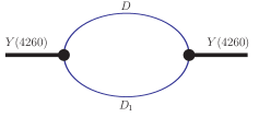
Here, is the derivative of the transverse part of the mass operator of the molecular states (see Fig. 1), which is defined as
| (7) |
The explicit expression for the coupling constant resulting from the compositeness condition is
| (8) | |||||
In the previous equation we use the notation
| (9) |
where , for and for , respectively.
In the calculation we use for the , the mass MeV and width MeV Coan:2006rv . The mass of the is expressed in terms of the constituent meson masses and the binding energy as
| (10) |
Note that is a variable quantity in our calculations, which we vary from 0.5 to 5 MeV. Once the mass of the composite state is fixed, the value for the coupling of to can be extracted from the compositeness condition. Values for this coupling in dependence on the binding energy and the cutoff are shown in Table I. Note that the dependence of on the binding energy is in agreement with the scaling law of hadronic molecules found in Ref. Branz:2008cb : . Moreover, for the central mass value of the Y(4260), the couplings of Y(4260) to are 7.85 for GeV and 6.25 for GeV, respectively.
Table I. Results for the coupling constant depending on and .
| in GeV | in MeV | |||
|---|---|---|---|---|
| 0.5 | 1 | 2.5 | 5 | |
| 0.5 | 2.2 | 2.3 | 2.6 | 3.1 |
| 0.75 | 2.1 | 2.2 | 2.5 | 2.9 |
Table II. Decay widths for in MeV.
| in MeV | in GeV | |||
|---|---|---|---|---|
| (0.5,0.5) | (0.5,0.75) | (0.75,0.5) | (0.75,0.75) | |
| 0.5 | ||||
| 1 | ||||
| 2.5 | ||||
| 5 | ||||
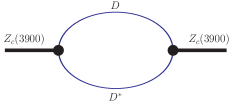
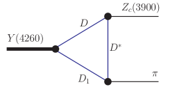
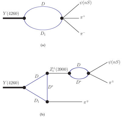
The diagram contributing to the two-body decays is shown in Fig. 2. The diagrams contributing to the transition are drawn in Fig. 3: the contact diagram [Fig. 3(a)] and the resonance diagram [Fig. 3(b)]. For the decays, as presented by the diagrams of Figs. 2 and 3, additional dynamical input is needed. To calculate the two-body decays (Fig. 2) and the resonance diagram corresponding to the transition (see Fig. 3(b)), we use the phenomenological Lagrangian for the coupling with
| (11) |
where and are the stress tensors of and mesons. The coupling can be estimated by considering the decay width of of MeV (see details in Ref. Branz:2010sh ) which is 2/3 of the total width. Then one gets GeV-1.
For the evaluation of the contact diagram in Fig. 3(a), we also need the interaction Lagrangian which can be derived using formalism proposed in Ref. Dong:2013iqa . In particular, one can derive a phenomenological Lagrangian describing the coupling of heavy quarkonia with pair of pseudoscalar, vector or axial heavy-light mesons and light pseudoscalar mesons. The phenomenological Lagrangian reads
| (12) |
where and are effective coupling constants, and denote the commutator and anticommutator, respectively.
The is the heavy charmonia field; is the superposition of isodoublets of open-charm mesons with and ; is the chiral field:
| (13) | |||||
| (14) | |||||
| (15) |
where and denote the and states; is the stress tensor of the and states; is a phenomenological coupling defining the mixing of derivative and nonderivative terms in ; is associated with the mass; , are the doublets of pseudoscalar and vector charmed mesons; is the chiral vielbein:
| (16) |
where MeV is the pion decay constant, is the triplet of pions. Note the couplings , and are phenomenological parameters. Below we show that we have two constraints on these couplings.
From Eq. (12) we deduce specific Lagrangians describing the couplings between heavy charmonia, charmed mesons and the pion which are relevant for the decay
| (17) |
In the evaluation of Fig. 3(b) the subprocess is treated as worked out in Ref. Dong:2013iqa .
III Decay modes and results
The two-body decay width for the transition described in Fig. 2 is given by
| (18) |
where is the magnitude of the three-momentum of outgoing particles in the rest frame of the state,
| (19) |
is the Källen function and is the corresponding invariant matrix element. We consider the finite width of the Y(4260) by setting up a mass distribution in the form Dover:1990kn ; Gutsche:2008qq
| (25) |
The lowest strong decay threshold is denoted by GeV, and is a normalization constant such that
| (26) |
In Eq. (13) we average the available phase space over the mass distribution of the , while the matrix element is evaluated at the central mass value of MeV. This procedure will capture the major features of the mass distribution of the .
The three-body decay width related to the process of Fig. 3 is evaluated as
| (27) |
where and are the momenta and masses of the three outgoing particles; and are the Mandelstam variables,
| (28) |
Again, the invariant matrix element of the three-body decay is simply denoted by , which is estimated at the central mass MeV. The calculation of phase space includes the mass distribution of the . The evaluation of the invariant matrix elements in both the two- and three-body decay is standard and not explicitly written out. The calculational technique is, for example, discussed in detail in Ref. Dong:2013iqa .
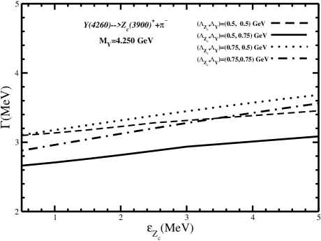
The diagram contributing to the two-body decay is shown in Fig. 2. Numerical results for , which are of the order of a few MeV, are given both in Table II and Fig. 4. In our calculations we use two different values for the cutoff parameters and — and GeV. The dependence of the decay width on the size parameter is only moderate. A larger binding energy leads to an increase in phase space and hence in the decay width.
Table III. decay widths in MeV.
Predictions for the mode with are given in brackets.
For total width of , we use BESIII data MeV Ablikim:2013mio .
| in MeV | in GeV | |||
|---|---|---|---|---|
| (0.5,0.5) | (0.5,0.75) | (0.75,0.5) | (0.75,0.75) | |
| 0.5 | ||||
| () | () | () | () | |
| 1 | ||||
| () | () | () | () | |
| 2.5 | ||||
| () | () | () | () | |
| 5 | ||||
| () | () | () | () | |
Table IV. decay widths in MeV.
Predictions for the mode with are given in brackets.
For total width of , we use Belle data ( MeV) Liu:2013dau .
| in MeV | in GeV | |||
|---|---|---|---|---|
| (0.5,0.5) | (0.5,0.75) | (0.75,0.5) | (0.75,0.75) | |
| 0.5 | ||||
| () | () | () | () | |
| 1 | ||||
| () | () | () | () | |
| 2.5 | ||||
| () | () | () | () | |
| 5 | ||||
| () | () | () | () | |
Table V. Contribution of the contact diagram in Fig. 3(a)
to in MeV.
| Mode | GeV | GeV |
|---|---|---|
In Tables III and IV we present our numerical results for the widths of both decay modes involving and (in brackets). Results are given for different values of the binding energy and of the respective size parameters and . In the calculation of the resonance contribution, the propagator of state is described by a Breit–Wigner form, where we have used a constant width in the imaginary part, i.e. we have used
| (29) |
We consider two results for including error bars: MeV — according to BESIII Ablikim:2013mio (see Table III) and — MeV — the result of the Belle Collaboration Liu:2013dau (see Table IV). The results for the sole contribution of the contact diagram in Fig. 3(a) are shown in Table V.
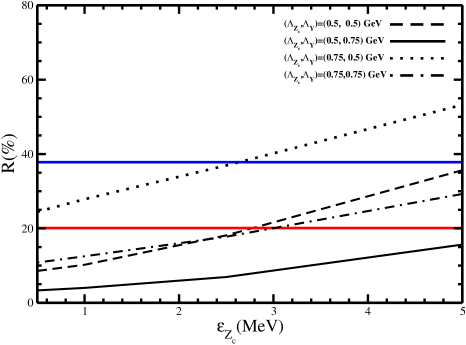
For completeness we also plot our results for the three-body decays in Figs. 5-7. In particular, in Fig. 5 we plot the ratio of resonance diagram [Fig. 3(b)] to total contribution (Fig. 3) to the decay width as a function of the binding energy MeV and for different cutoff parameters GeV. The two horizontal lines at and define the lower and upper limit set by data of the Belle Collaboration Liu:2013dau ,
| (30) |
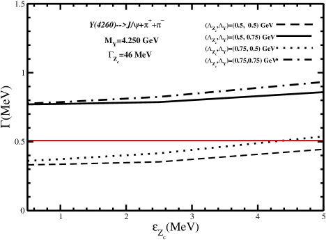
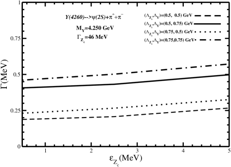
As is evident from Fig. 5, the ratio is rather sensitive to explicit values of the binding energy and the choice of size parameters. The present range of values set by Belle can be reproduced in the calculation for restricted values of the varied quantities. In Figs. 6 and 7 we plot the total contributions to the decay rates of and . In Fig. 6 we indicate the horizontal line MeV corresponding to the lower limit for this decay rate extracted from data of Ref. Mo:2006ss . From this constraint and from data for the ratio we estimate that the lower limit of is larger than 100 keV. Using the last constraint and the results for the ratio , we conclude that for a favored value of GeV we deduce a lower limit of MeV. Our results for the favored value of GeV and including the variation of the cutoff parameter and of the binding energy can be summarized as
| (31) | |||||
In summary, using a phenomenological Lagrangian approach, we give predictions for the two- and three-body decay rates and for . Our results for the two-body decays are in the order of several MeV. For the three-body decay with a charged pion pair, we estimated both contact and -resonance contributions, and the decay rate varies from several hundred keV to a few MeV. Both the background and contributions are explicitly shown. We expect that the quantitative predictions given here can serve as a further test for the molecular interpretation of the and can be measured in forthcoming experiments.
In further work we plan to estimate other strong and also radiative decay modes of the state. In particular, the following decay modes of the state can be analyzed: strong decay modes with two heavy charm mesons , or in the final state, the strong decay modes with a state, and radiative decay . Special attention will be paid to an analysis of other possible hidden charm resonances [in addition to ] with spin-parities and with a mass in the interval MeV, all contributing to the total width of the state.
Acknowledgements.
We thank Alex Bondar, Qiang Zhao, Dian Yong Chen and Changzheng Yuan for useful discussions. This work is supported by the DFG under Contract No. LY 114/2-1, the National Sciences Foundations of China No.10975146 and No.11035006, and by the DFG and the NSFC through funds provided to the sino-German CRC 110 “Symmetries and the Emergence of Structure in QCD.” The work is done partially under the Project No. 2.3684.2011 of Tomsk State University. V. E. L. would like to thank Tomsk Polytechnic University, Russia for warm hospitality. Y. B. D. thanks the Institute of Theoretical Physics, University of Tübingen, for warm hospitality and the Alexander von Humboldt Foundation for support.References
- (1) M. Ablikim et al. [ BESIII Collaboration], Phys. Rev. Lett. 110, 252001 (2013) [arXiv:1303.5949 [hep-ex]].
- (2) Z. Q. Liu et al. [Belle Collaboration], Phys. Rev. Lett. 110, 252002 (2013) [arXiv:1304.0121 [hep-ex]].
- (3) T. Xiao, S. Dobbs, A. Tomaradze and K. K. Seth, arXiv:1304.3036 [hep-ex].
- (4) F. -K. Guo, C. Hidalgo-Duque, J. Nieves and M. P. Valderrama, Phys. Rev. D 88, 054007 (2013) [arXiv:1303.6608 [hep-ph]]. D. -Y. Chen, X. Liu and T. Matsuki, Phys. Rev. Lett. 110, 232001 (2013) [arXiv:1303.6842 [hep-ph]]; R. Faccini, L. Maiani, F. Piccinini, A. Pilloni, A. D. Polosa and V. Riquer, Phys. Rev. D 87, 111102 (2013) [arXiv:1303.6857 [hep-ph]]: M. Karliner and S. Nussinov, JHEP 1307, 153 (2013) [arXiv:1304.0345 [hep-ph]]; N. Mahajan, arXiv:1304.1301 [hep-ph]; C. -Y. Cui, Y. -L. Liu, W. -B. Chen and M. -Q. Huang, Eur. Phys. J. C 73, 2661 (2013) [arXiv:1304.1850 [hep-ph]]; Q. Wang, C. Hanhart and Q. Zhao, Phys. Rev. Lett. 111, 132003 (2013) [arXiv:1303.6355 [hep-ph]]; M. B. Voloshin, Phys. Rev. D 87, 091501 (2013) [arXiv:1304.0380 [hep-ph]]; E. Wilbring, H. -W. Hammer and U. -G. Meißner, Phys. Lett. B 726, 326 (2013) [arXiv:1304.2882 [hep-ph]]; G. Li, Eur. Phys. J. C 73, 2621 (2013) [arXiv:1304.4458 [hep-ph]]; J. -R. Zhang, Phys. Rev. D 87, 116004 (2013) [arXiv:1304.5748 [hep-ph]]. D. -Y. Chen, X. Liu and T. Matsuki, Phys. Rev. D 88, 036008 (2013) [arXiv:1304.5845 [hep-ph]]. J. M. Dias, F. S. Navarra, M. Nielsen and C. M. Zanetti, Phys. Rev. D 88, 016004 (2013) [arXiv:1304.6433 [hep-ph]]. E. Braaten, arXiv:1305.6905 [hep-ph].
- (5) Y. Dong, A. Faessler, T. Gutsche and V. E. Lyubovitskij, Phys. Rev. D 88, 014030 (2013) [arXiv:1306.0824 [hep-ph]].
- (6) B. Aubert et al. [BaBar Collaboration], Phys. Rev. Lett. 95, 142001 (2005) [hep-ex/0506081].
- (7) S. R. Blusk, AIP Conf. Proc. 870, 341 (2006).
- (8) K. Abe et al. [Belle Collaboration], hep-ex/0612006.
- (9) S. -L. Zhu, Phys. Lett. B 625, 212 (2005) [hep-ph/0507025].
- (10) G. -J. Ding, Phys. Rev. D 79, 014001 (2009) [arXiv:0809.4818 [hep-ph]].
- (11) Q. Wang, C. Hanhart and Q. Zhao, Phys. Rev. Lett. 111, 132003 (2013) [arXiv:1303.6355 [hep-ph]].
- (12) A. Martinez Torres, K. P. Khemchandani, D. Gamermann and E. Oset, Phys. Rev. D 80, 094012 (2009) [arXiv:0906.5333 [nucl-th]].
- (13) X. Liu, X. -Q. Zeng and X. -Q. Li, Phys. Rev. D 72, 054023 (2005) [hep-ph/0507177].
- (14) C. Z. Yuan, P. Wang and X. H. Mo, Phys. Lett. B 634, 399 (2006) [hep-ph/0511107].
- (15) F. J. Llanes-Estrada, Phys. Rev. D 72, 031503 (2005) [hep-ph/0507035].
- (16) L. Maiani, V. Riquer, F. Piccinini and A. D. Polosa, Phys. Rev. D 72 (2005) 031502 [hep-ph/0507062].
- (17) T. -W. Chiu et al. [TWQCD Collaboration], Phys. Rev. D 73, 094510 (2006) [hep-lat/0512029].
- (18) J. M. Dias, R. M. Albuquerque, M. Nielsen and C. M. Zanetti, Phys. Rev. D 86, 116012 (2012) [arXiv:1209.6592 [hep-ph]].
- (19) D. -Y. Chen, J. He and X. Liu, Phys. Rev. D 83, 054021 (2011) [arXiv:1012.5362 [hep-ph]].
- (20) E. Kou and O. Pene, Phys. Lett. B 631, 164 (2005) [hep-ph/0507119].
- (21) F. Iddir and L. Semlala, hep-ph/0611183.
- (22) C. -F. Qiao, Phys. Lett. B 639, 263 (2006) [hep-ph/0510228].
- (23) E. van Beveren and G. Rupp, hep-ph/0605317.
- (24) F. Close and C. Downum, Phys. Rev. D 79, 014027 (2009) [arXiv:0809.3419 [hep-ph]].
- (25) A. Faessler, T. Gutsche, V. E. Lyubovitskij and Y. -L. Ma, Phys. Rev. D 76, 014005 (2007) [arXiv:0705.0254 [hep-ph]]; Phys. Rev. D 76, 114008 (2007) [arXiv:0709.3946 [hep-ph]]; Phys. Rev. D 77, 114013 (2008) [arXiv:0801.2232 [hep-ph]]; A. Faessler, T. Gutsche, S. Kovalenko and V. E. Lyubovitskij, Phys. Rev. D 76, 014003 (2007) [arXiv:0705.0892 [hep-ph]]; Y. Dong, A. Faessler, T. Gutsche and V. E. Lyubovitskij, Phys. Rev. D 77, 094013 (2008) [arXiv:0802.3610 [hep-ph]]; Phys. Rev. D 79, 094013 (2009) [arXiv:0903.5416 [hep-ph]].
- (26) T. Branz, T. Gutsche and V. E. Lyubovitskij, Phys. Rev. D 79, 014035 (2009) [arXiv:0812.0942 [hep-ph]].
- (27) T. Branz, T. Gutsche and V. E. Lyubovitskij, Phys. Rev. D 80, 054019 (2009) [arXiv:0903.5424 [hep-ph]].
- (28) T. Branz, T. Gutsche and V. E. Lyubovitskij, Phys. Rev. D 82, 054025 (2010) [arXiv:1005.3168 [hep-ph]].
- (29) Y. Dong, A. Faessler, T. Gutsche and V. E. Lyubovitskij, J. Phys. G 38, 015001 (2011) [arXiv:0909.0380 [hep-ph]].
- (30) Y. Dong, A. Faessler, T. Gutsche and V. E. Lyubovitskij, Phys. Rev. D 81, 014006 (2010) [arXiv:0910.1204 [hep-ph]]; Y. Dong, A. Faessler, T. Gutsche and V. E. Lyubovitskij, Phys. Rev. D 81, 074011 (2010) [arXiv:1002.0218 [hep-ph]]; Y. Dong, A. Faessler, T. Gutsche, S. Kumano and V. E. Lyubovitskij, Phys. Rev. D 82, 034035 (2010) [arXiv:1006.4018 [hep-ph]]; Phys. Rev. D 83, 094005 (2011) [arXiv:1103.4762 [hep-ph]].
- (31) Y. Dong, A. Faessler, T. Gutsche and V. E. Lyubovitskij, J. Phys. G 40, 015002 (2013) [arXiv:1203.1894 [hep-ph]].
- (32) S. Weinberg, Phys. Rev. 130, 776 (1963); A. Salam, Nuovo Cim. 25, 224 (1962); K. Hayashi, M. Hirayama, T. Muta, N. Seto and T. Shirafuji, Fortsch. Phys. 15, 625 (1967).
- (33) G. V. Efimov and M. A. Ivanov, The Quark Confinement Model of Hadrons, (IOP Publishing, Bristol Philadelphia, 1993).
- (34) I. V. Anikin, M. A. Ivanov, N. B. Kulimanova and V. E. Lyubovitskij, Z. Phys. C 65, 681 (1995); M. A. Ivanov, M. P. Locher and V. E. Lyubovitskij, Few Body Syst. 21, 131 (1996); M. A. Ivanov, V. E. Lyubovitskij, J. G. Körner and P. Kroll, Phys. Rev. D 56, 348 (1997) [arXiv:hep-ph/9612463]; S. Dubnicka, A. Z. Dubnickova, M. A. Ivanov and J. G. Korner, Phys. Rev. D 81, 114007 (2010) [arXiv:1004.1291 [hep-ph]]; T. Gutsche, M. A. Ivanov, J. G. Korner, V. E. Lyubovitskij and P. Santorelli, Phys. Rev. D 86, 074013 (2012) [arXiv:1207.7052 [hep-ph]]; Phys. Rev. D 87, 074031 (2013) [arXiv:1301.3737 [hep-ph]].
- (35) T. E. Coan et al. [CLEO Collaboration], Phys. Rev. Lett. 96, 162003 (2006) [hep-ex/0602034].
- (36) C. B. Dover, T. Gutsche and A. Faessler, Phys. Rev. C 43, 379 (1991).
- (37) T. Gutsche, V. E. Lyubovitskij and M. C. Tichy, Phys. Rev. D 79, 014036 (2009) [arXiv:0811.0668 [hep-ph]].
- (38) X. H. Mo et al., Phys. Lett. B 640, 182 (2006) [hep-ex/0603024].