A method to compute periodic sums

Abstract

In a number of problems in computational physics, a finite sum of kernel functions centered at $N$ particle locations located in a box in three dimensions must be extended by imposing periodic boundary conditions on box boundaries. Even though the finite sum can be efficiently computed via fast summation algorithms, such as the fast multipole method (FMM), the periodized extension is usually treated via a different algorithm, Ewald summation, accelerated via the fast Fourier transform (FFT). A different approach to compute this periodized sum just using a blackbox finite fast summation algorithm is presented in this paper. The method splits the periodized sum in to two parts. The first, comprising the contribution of all points outside a large sphere enclosing the box, and some of its neighbors, is approximated inside the box by a collection of kernel functions (“sources”) placed on the surface of the sphere or using an expansion in terms of spectrally convergent local basis functions. The second part, comprising the part inside the sphere, and including the box and its immediate neighborhood, is treated via available summation algorithms. The coefficients of the sources are determined by least squares collocation of the periodicity condition of the total potential, imposed on a circumspherical surface for the box. While the method is presented in general, details are worked out for the case of evaluating electrostatic potentials and forces. Results show that when used with the FMM, the periodized sum can be computed to any specified accuracy, at an additional cost of the order of the free-space FMM. Several technical details and efficient algorithms for auxiliary computations are provided, as are numerical comparisons.

Keywords

periodic sums; fast multipole method; Ewald summation; GPU computing; kernel independent methods; molecular dynamics; long-range interactions

Acknowledgments

Work partially supported by the following sources: AFOSR under MURI Grant W911NF0410176 (PI Prof. J. G. Leishman, monitor Dr. D. Smith); by NSF award 1250187 (PI: Prof. B. Balachandran); by Grant G34.31.0040 (PI: Prof. I. Akhatov) of the Russian Ministry of Education & Science.; and by Fantalgo, LLC.

1 Introduction

Many problems in physics, chemistry and materials science lead to a free-space finite “particle” sum of $N$ functions, $K$, centered at locations $\mathbf{x}_{i}$ $\in\Omega_{0}\subset\mathbb{R}^{3}$, where $\Omega_{0}$ is a rectangular box $d_{1}\times d_{2}\times d_{3}$ centered at the origin of the reference frame

$$\tilde{\phi}\left(\mathbf{y}\right)=\sum_{i=1}^{N}q_{i}K\left(\mathbf{y}-\mathbf{x}_{i}\right).$$ (1)

For evaluation at $N$ locations $\mathbf{y}$, this sum has a quadratic cost. There are efficient and arbitrarily accurate approximation algorithms for this summation (e.g., the fast multipole method, FMM [6]).

Often, an extension to this sum for $\tilde{\phi}$ must be computed in which periodic boundary conditions are enforced on box boundaries, resulting in the potential $\phi$. This can be evaluated by replacing the sum (1) with the infinite sum

$$\phi\left(\mathbf{y}\right)=\sum_{\mathbf{p}}\sum_{i=1}^{N}q_{i}K\left(\mathbf{y}-\mathbf{x}_{i}+\mathbf{p}\right),\quad\mathbf{p}\in\mathbb{P}=\left\{\left(i_{1}d_{1},i_{2}d_{2},i_{3}d_{3}\right):\left(i_{1},i_{2},i_{3}\right)\in\mathbb{Z}^{3}\right\}.$$ (2)

For some functions $K$, such as those representing the field of an electrostatic charge, this infinite sum may be divergent or conditionally convergent. In this case certain side conditions may be needed to compute a physically relevant sum. Usually such infinite sums are performed using Fourier-transform based Ewald summation [1], which is accelerated via the FFT. This method is described briefly in Appendix D. Accounting for all pairwise interactions the method can achieve $O(N\log N)$ complexity, for $N$ particles in the box $\Omega_{0}$ which is periodically replicated over the full space [2, 3]. Because of the technique used for grid-to-particle interpolation these methods are usually low-order. A high-order accurate Gaussian interpolation based Ewald summation algorithm was recently presented in [4, 5].

Another scalable algorithm, which can be employed for computation of periodic sums (2) is the FMM. A criticism of FMM algorithms has been that they are relatively harder to implement, combining the need for efficient data structures, careful analysis and computation of special functions, and mixed memory access patterns. Nevertheless, several open-source and commercial packages implementing the FMM for standard kernels in free space have become available. The FMM is used less often in practice to compute periodic sums, even though several methods to handle periodic boundary conditions using extensions to the basic FMM have been proposed, starting from the first publication of the algorithm [6, 7, 8, 9, 10, 11, 12, 13, 14, 15, 16]. Some authors (e.g. [12]) claim that the overhead in the FMM for computation of periodic sums can be negligibly small. This is true under a few conditions, but not in others. This is discussed in detail in a section entitled Discussion. Analysis of the FMM and its plane-wave variant, which is better-suited tor large $N$ and parallel architectures than the smooth particle mesh Ewald algorithm, is presented in [17]. However, all these methods require constructing a new and different algorithm – a periodic variant, for which optimized implementations are not in general available. Furthermore, some of these algorithms may not extend easily to non-cubic domains.

It can be mentioned in this context that any FMM has a so-called break-even point, $N_{b}$, such that at $N<N_{b}$ brute force summation (1) is faster than the FMM computation. The value of $N_{b}$ depends on the method used, implementation, required accuracy (the FMM is an approximate algorithm), and hardware. It may vary in a range $N_{b}\sim 10^{2}-10^{4}$, which is of the order of $N$ for some practical problems (e.g. for some molecular dynamics simulations). In such cases, the use of periodic FMM just for the purpose of computing of infinite sums (2) even if the overhead for periodization will be zero is questionable if some other periodization method, which can use finite brute force summation algorithms is available.

Special purpose hardware such as graphics processors or heterogeneous CPU/GPU architectures also allow the fast computation of finite sums, either via brute force summation [18], or via the mapping of the FMM onto these architectures [19, 20, 21, 22]. Yokota et al. [22] favorably compare a large scale FMM-based vortex element computations with a direct numerical simulation via periodic pseudospectral methods. Their simulations could have been faster and more accurate – the FMM was executed on a finite system composed of 3³ images, which while not being truly periodic also makes using the FMM significantly more expensive.

The problem this paper seeks to address is: Given a black-box fast summation algorithm (FSA) for computing finite sums with a given kernel $K\left(\mathbf{y}-\mathbf{x}_{i}\right)$ that is available to the user, is it possible to compute the same sum with periodic boundary conditions without any modification of the FSA? We provide a positive answer to this question. Our algorithm has the same cost as the FSA, and can be computed to any user specified accuracy $\epsilon$, and does not use the FFT. The basic idea of the method is to divide the sum (2) in to two parts. One part computes a finite sum of particles that lie within a sphere centered at the box. This is computed using the available FSA. The other part, is an approximation of the field within the box due to all particles outside the sphere. The field due to these sources can be represented within the box in terms of local expansions. Such local expansions have also been proposed in other attempts to extend the FMM to periodic systems, but are there derived by explicit translation of multipole expansions from outside the box of interest into it. In our method, we propose to determine the coefficients directly from the periodicity conditions on the potential, which results in solution of a relatively small overdetermined function-fitting problem, easily solved via standard algorithms – e.g., rank-revealing $QR$ decomposition. This step is in the spirit of the “kernel-independent” FMM methods [26, 27]. In this context we should mention Ref. [15]. Even though it is dedicated to the Helmholtz equation in two dimensions, a method for “periodization” of free-space solutions similar in spirit to that presented here was proposed and tested. Moreover, the cited paper contains an additional “periodization” method based on boundary integrals, which can be tried for different kernels and space dimensionality (also see [28], where periodization along one dimension is performed).

We present this “periodization” approach in a general setting, but focus computational examples on the evaluation of the electrostatic potential $\phi$ and its gradient $\nabla\phi$ at $M$ evaluation points $\mathbf{y}_{j}$ $\in\Omega_{0}\subset\mathbb{R}^{3}$ due to $N$ charged particles of charge $q_{i}$ placed in $\Omega_{0}$, and subject to periodic boundary conditions on $\partial\Omega_{0}$. This reduces to computing the infinite, conditionally convergent, sum (1), with kernel function $K$:

$$K\left(\mathbf{y}-\mathbf{x}\right)=\frac{1}{\left|\mathbf{y}-\mathbf{x}\right|},\quad\mathbf{y}\neq\mathbf{x;\quad}K\left(\mathbf{y}-\mathbf{x}\right)=0,\quad\mathbf{y}=\mathbf{x},\qquad\sum_{i=1}^{N}q_{i}=0.$$ (3)

and the net charge in each box being zero. Of course, in practical applications, such as in molecular dynamics, there will be other computations beyond the sum necessary to stabilize the overall computations. This paper does not consider these, focusing on the electrostatic sum at a single time step.

The periodization method could be easily applied to other kernels for which a “fast summation algorithm” (FSA) is available. As long as the periodic sum makes sense, and the kernel $K$ can be expanded over some local basis, the proposed method should work. Conditions similar to the charge neutrality in (3) may be necessary. The proposed method can also be applied for 2D problems, though we present it in 3D. Also, the periodic extension of the computational domain (box) may be performed only along one or two coordinates, for which Ewald summation may have problems.

2 Proposed method

2.1 Periodization

The box on which the periodic sum is to be computed is denoted $\Omega_{0}$. Let $S_{0}$ be a ball of radius $R_{0}$ centered at the center of the box $\Omega_{0}$ and containing it. Let $S_{b}$ be another ball with the same center and radius $R_{b}>R_{0}$ (see Fig. 1). We denote as $\Omega_{b}$ a finite region which includes the ball $S_{b}$ (the minimal $\Omega_{b}$ is the ball $S_{b}$). We decompose the infinite sum as

$$\phi\left(\mathbf{y}\right)=\phi_{near}\left(\mathbf{y}\right)+\phi_{far}\left(\mathbf{y}\right),\quad\phi_{near}\left(\mathbf{y}\right)=\sum_{\mathbf{x}_{j}\in\Omega_{b}}q_{j}K\left(\mathbf{y}-\mathbf{x}_{j}\right),\quad\phi_{far}\left(\mathbf{y}\right)=\sum_{\mathbf{x}_{j}\notin\Omega_{b}}q_{j}K\left(\mathbf{y}-\mathbf{x}_{j}\right),$$ (4)

where $\phi_{near}\left(\mathbf{y}\right)$ is to be computed using the FSA (assumed to be the FMM in the sequel) to the specified accuracy $\epsilon$ while $\phi_{far}\left(\mathbf{y}\right)$ is computed by some other method at least to the same accuracy. The sources in the infinite domain are indexed as $\mathbf{x}_{j}=\mathbf{x}_{i}-\mathbf{p}$, $q_{j}=q_{i}$ for appropriate vectors $\mathbf{p\in}$ $\mathbb{P}$ (see Eq. (2)).

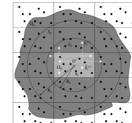
Figure 1: The particle sum (2) in the box $\Omega_{0}$, subject to periodic boundary conditions on the box boundary, is to be computed to a specified accuracy $\epsilon$. The boundary condition can be enforced by the image method, which results in an infinite set of copies of the box $\Omega_{0}$. The proposed method divides the sum into a near-field component in $\Omega_{b}$ and a far-field sum.

To apply the FMM to the kernel function $K\left(\mathbf{y}\right)$ it should be possible to approximate it via a convergent series over a set of local basis functions $\left\{R_{t}\left(\mathbf{y}\right)\right\}$. This means that for any source point $\mathbf{x}_{j}\notin\Omega_{b}$ we have the factorization

$$K\left(\mathbf{y}-\mathbf{x}_{j}\right)=\sum_{t=1}^{P}B_{t}\left(\mathbf{x}_{j}\right)R_{t}\left(\mathbf{y}\right)+\epsilon_{j}^{(P)},\quad\left|\mathbf{x}_{j}\right|>R_{b},\quad\left|\mathbf{y}\right|<R_{0},$$ (5)

where $P$ is the number of terms retained in the infinite series, $B_{t}\left(\mathbf{x}_{j}\right)$ are the expansion coefficients, and $\epsilon_{j}^{(P)}$ is the truncation error depending on $\left|\mathbf{x}_{j}\right|$ and $R_{0}$. The basis functions can be some standard choices, or, as in the kernel independent FMM [27], can be taken to be a collection of kernel functions, centered outside the region of approximation

$$R_{t}\left(\mathbf{y}\right)=K\left(\mathbf{y}-\mathbf{x}_{t}^{(s)}\right),\quad\left|\mathbf{x}_{t}^{(s)}\right|>R_{b},$$ (6)

where $\mathbf{x}_{t}^{(s)}$ are a collection of sources located outside ball $S_{b}$. This method has the flavor of “equivalent-source” methods. Since the function $K$ depends only on the distance between its argument, it is a “radial basis function”, or RBF [24]. While any approximation scheme may be used, the use of kernel $K$ as RBF is dictated by the fact that this kernel satisfies the underlying equation (e.g. the Laplace equation), so the approximation to the field via the sum of such RBFs also satisfies the equation (if it is linear and space invariant). Substituting Eq. (5) into the expression for $\phi_{far}\left(\mathbf{y}\right)$ from Eq. (4), we obtain

$$\phi_{far}\left(\mathbf{y}\right) = \sum_{t=1}^{P}C_{t}R_{t}\left(\mathbf{y}\right)+\epsilon^{(P)},\quad$$ (7)

$$C_{t} = \sum_{\mathbf{x}_{j}\notin\Omega_{b}}q_{j}B_{t}\left(\mathbf{x}_{j}\right),\quad\epsilon^{(P)}=\sum_{\mathbf{x}_{j}\notin\Omega_{b}}q_{j}\epsilon_{j}^{(P)}.$$

A necessary condition for our method is convergence of both infinite sums $C_{t}$ and $\epsilon^{(P)}$. The problem of computation of $\phi_{far}\left(\mathbf{y}\right)$ has been reduced to that of determination of $P$ fitting coefficients $C_{t}$. These can be determined via least-squares collocation as follows. Consider a set of $L>P$ check points, $\mathbb{Y}^{(c)}\subset S_{0}\backslash\Omega_{0}$. A point $\mathbf{y}_{l}^{(c)}\in\mathbb{Y}^{(c)}$ has two properties:first,$\left|\mathbf{y}_{l}^{(c)}\right|<R_{0}$, and, second, that there exists $\mathbf{p\in}\mathbb{P}$ such that point $\widetilde{\mathbf{y}}_{l}^{(c)}=\mathbf{y}_{l}^{(c)}+\mathbf{p}\in S_{0}$ (see Fig. 1). This means that

$$\phi\left(\mathbf{y}_{l}^{(c)}\right)=\phi\left(\widetilde{\mathbf{y}}_{l}^{(c)}\right),\quad l=1,...,L.$$ (8)

In terms of decomposition (4) and representation of the far field (7) this system can be rewritten as

$$\sum_{t=1}^{P}A_{lt}C_{t} = f_{l}+\epsilon_{l}^{(P)},\quad l=1,...,L,$$ (9)

$$A_{lt} = R_{t}\left(\mathbf{y}_{l}^{(c)}\right)-R_{t}\left(\widetilde{\mathbf{y}}_{l}^{(c)}\right),\quad f_{l}=\phi_{near}\left(\widetilde{\mathbf{y}}_{l}^{(c)}\right)-\phi_{near}\left(\mathbf{y}_{l}^{(c)}\right)$$

where $\left|\epsilon_{l}^{(P)}\right|=\left|\epsilon^{(P)}\left(\widetilde{\mathbf{y}}_{l}^{(c)}\right)-\epsilon^{(P)}\left(\mathbf{y}_{l}^{(c)}\right)\right|\leqslant 2\max_{\mathbf{y\in}S_{0}}\left|\epsilon^{(P)}\left(\mathbf{y}\right)\right|.$ We have $L$ linear equations in $P$ unknowns $C_{1},...,C_{P}$. As we are not constrained with the size of the set of the set points, $L>P$ can be selected to provide a substantial oversampling, so minimization of functional

$$F\left(C_{1},...,C_{P}\right)=\sum_{l=1}^{L}\left(\sum_{t=1}^{P}A_{lt}C_{t}-f_{l}\right)^{2},$$ (10)

should take care about the “noise” introduced into the approximation due to $\epsilon_{l}^{(P)}$. The least square minimization procedure is well known and formally it results in solution

$$\mathbf{C=A}^{\dagger}\mathbf{f,\quad A}^{\dagger}=\left(\mathbf{A}^{T}\mathbf{A}\right)^{-1}\mathbf{A}^{T},$$ (11)

where $\mathbf{C=}\left\{C_{t}\right\}$ and $\mathbf{f=}\left\{f_{l}\right\}$ are organized as column vectors of size $P$ and $L$, respectively and $\mathbf{A}^{\dagger}$ is the $P\times L$ matrix, which is the pseudoinverse of $\mathbf{A}$, and superscript $T$ denotes transposition. Note that this notation is formal, and is not the way the least-squares problem is solved in practice. Rather a stable algorithm such as the rank-revealing QR decomposition [32] is used, while it is strongly recommended to precompute and store matrix decompositions in the “set” part of the algorithm to reduce the cost of the “get” part.

The known coefficients $\mathbf{C}$ allow computation of $\phi_{far}\left(\mathbf{y}\right)$ and can be added to the $\phi_{near}$ obtained via the FSA. However, some technical details need to be specified. In the next section we provide analysis and details for the important case of the Coulombic kernel (2).

A similar collocation of kernel based RBF expansions at a relatively small amount of the check points is also used in the “kernel independent” FMM [26] with basis functions (6). There, the collocation is at the level of the boxes in the FMM octree data structure, and fitting takes the place of expansions and translations. Here, we collocate the differences of the overall solution at a set of check points $\mathbf{y}_{l}^{(c)}$ and at their periodic images $\widetilde{\mathbf{y}}_{l}^{(c)}$, at the level of the overall domain to determine the expansion coefficients for $\phi_{far}$.

2.2 Check point set

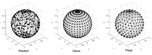
Figure 2: The check point distributions over the surface of a unit sphere for $p=16$: random distribution ($L=3p^{2}$ points), the Gauss spherical grid ($L=2p^{2}-p$), and the Thomson points ($L=p^{2}$).

Selection of an optimal set of check points $\mathbb{Y}^{(c)}\subset S_{0}\backslash\Omega_{0}$ is not trivial. A good check point set should yield a well conditioned solution, and sample the solution well spatially. A simple way which does not yield such a well conditioned set is to select the points $\mathbf{y}_{l}^{(c)}\in\mathbb{Y}^{(c)}$ on the boundary of box $\Omega_{0}$. This is because the corresponding periodic point $\widetilde{\mathbf{y}}_{l}^{(c)}$ will then also be located on the box boundary on the face opposite to $\mathbf{y}_{l}^{(c)}$. In this case the distances from the box center to $\mathbf{y}_{l}^{(c)}$ and to $\widetilde{\mathbf{y}}_{l}^{(c)}$ will be the same, so both points will be located on a sphere of radius $r_{l}^{(c)}$. If the basis is based on spherical functions, then several of these will take the same value for symmetrical points on the sphere, and the fitting equations may be rank deficient.

To avoid this degeneracy, the set $\mathbb{Y}^{(c)}$ was chosen from points on the surface of ball $S_{0}$. Three distributions were tried (see Fig. (2): i) random uniformly distributed points, ii) Gaussian nodes (zeros of the Legendre polynomial along $\theta$, $P_{p}\left(\cos\theta\right)$, see [33]) and equispaced with respect to $\varphi$), and, iii) the almost uniform distribution of points over the sphere obtained by solving the so-called Thomson problem of the equilibrium position of mutually repelling electrons constrained to be on the surface of the sphere [34], see [35]. Methods ii) and iii) show better results than the random distribution, as shown in Section 3. Further, we fond that using the Thomson points for the interpolation in Eq. 6 provides good accuracy.

2.3 Periodization algorithm

The algorithm has two parts. In a first preliminary set-up step, denoted “set”, the check points are determined, and the matrix decompositions necessary to compute the least squares fit with the matrix $\mathbf{A}$ in Eq. (11) are precomputed. In simulations where the domain $\Omega_{0}$ is fixed and the particles move, as in molecular dynamics, this matrix does not change, and the cost of the “set” step is amortized over the entire simulation. The second part of the algorithm, denoted “get,” computes the right hand side and solution of the fitting equations via an inexpensive step such as backsubstitution. The accuracy depends on the choice of basis functions, and the parameters $P$,$L$, and $R_{b}$. In the next section we provide both a theoretical and an empirical study for the case of the Coulombic kernel (Green’s function of Laplace’s equation).

2.3.1 Algorithm “set”

1. Set the circumsphere radius $R_{0}=\frac{1}{2}\sqrt{d_{1}^{2}+d_{2}^{2}+d_{3}^{2}}$. Based on the required accuracy determine $R_{b}$, $P$, and $L\geqslant P$.

2. Generate $L$ check points distributed over the surface of the ball $S_{0}$, $\mathbf{y}_{l}^{(c)}\in\partial S_{0}$, $l=1,...,L.$ Denote this point set as $Y_{c1}$.

3. For each point $\mathbf{y}_{l}^{(c)}=\left(y_{l1}^{(c)},y_{l2}^{(c)},y_{l3}^{(c)}\right),$ $l=1,...,L,$ find a point $\widetilde{\mathbf{y}}_{l}^{(c)}\in S_{0}$, such that two Cartesian coordinates of $\widetilde{\mathbf{y}}_{l}^{(c)}$ are the same as those of the respective coordinates of $\mathbf{y}_{l}^{(c)}$, while the other coordinate, $\widetilde{y}_{lk}^{(c)}$ is shifted by $d_{k}$ with respect to $y_{lk}^{(c)}$. Denote $Y_{c2}$ $=\left\{\widetilde{\mathbf{y}}_{l}^{(c)}\right\}.$

4. Form the $L\times P$ fitting matrix $\mathbf{A=}\left\{A_{lt}\right\}$, $A_{lt}=R_{t}\left(\mathbf{y}_{l}^{(c)}\right)-R_{t}\left(\widetilde{\mathbf{y}}_{l}^{(c)}\right)$, $l=1,...,L,$ $t=1,...,P,$ where $R_{t}\left(\mathbf{y}\right)$ are the basis functions at the checkpoints.

5. Compute matrix decomposition of $\mathbf{A}$ necessary to solve the least squares problem.

6. (optional) Precompute other parameters which do not depend on the source distribution. If the summation needs certain auxiliary computations to ensure convergence, do those steps. For the Coulomb kernels this may involve computation of the integrals of the basis functions over the box $\Omega_{0}$.

2.3.2 Algorithm “get”

1. Periodically extend the source box $\Omega_{0}$ to cover the ball $S_{b}$ of radius $R_{b}$. The newly generated sources and charges will have coordinates $X_{\mathbf{p}}=\left\{\mathbf{x}_{i}+\mathbf{p}\right\}$ for the values of the periodization vector $\mathbf{p}_{1},...,\mathbf{p}_{b}$ from set $\mathbb{P}$ (see Eq. (2)) and charges $Q_{\mathbf{p}}=\left\{q_{i}\right\}.$ Denote the set of all sources as $X_{b}=X_{0}\cup X_{\mathbf{p}_{1}}\cup...\cup X_{\mathbf{p}_{b}}$. These constitute $\Omega_{b}$.

2. Find the set of $N_{b}$ sources $X_{near}$ by removing sources from the set $X_{b}$ that are outside the sphere $S_{b}$, and satisfy $\left|\mathbf{x}_{j}\right|>R_{b}$ $\left(X_{near}=\left\{\mathbf{x\in}X_{b}:\left|\mathbf{x}\right|\leqslant R_{b}\right\}\right).$

3. Using the FSA compute $\phi_{near}$ for a given set of evaluation points $Y_{0}=\left\{\mathbf{y}_{j}\right\},j=1,...,M$ residing in $\Omega_{0}$ and belonging to sets $Y_{c1}$ and $Y_{c2}$, i.e. for points from the set $Y=\left\{\mathbf{y\in}Y_{0}\cup Y_{c1}\cup Y_{c2}\right\}.$ If gradient computations are needed, compute $\nabla\phi_{near}$ at $\mathbf{y}_{j}\in Y_{0}.$

4. Form the right hand side of the periodization equation $\mathbf{f}$ $=\left\{f_{l}\right\},$ $f_{l}=\phi_{near}\left(\widetilde{\mathbf{y}}_{l}^{(c)}\right)-\phi_{near}\left(\mathbf{y}_{l}^{(c)}\right)$, $l=1,...,L,$ organized in a column vector.

5. Using the matrix decompositions in the “set” step solve the fitting equations for the $P$ expansion coefficients $\mathbf{C=}\left(C_{1},...,C_{P}\right)^{T}.$ This step can formally be written as $\mathbf{C}=$ $\mathbf{A}^{\dagger}\mathbf{f.}$

6. (optional) Compute the constant shift or other modification of the far field potential, if needed.

7. Evaluate $\phi_{far}\left(\mathbf{y}_{j}\right)$, and if gradient computation is needed, $\nabla\phi_{far}\left(\mathbf{y}_{j}\right)$, at $\mathbf{y}_{j}\in Y_{0}$.

8. Get the periodized solution of the problem, $\phi\left(\mathbf{y}_{j}\right)=\phi_{near}\left(\mathbf{y}_{j}\right)+\phi_{far}\left(\mathbf{y}_{j}\right),$ $\mathbf{y}_{j}\in Y_{0},$ and if gradient computation is needed, $\nabla\phi\left(\mathbf{y}_{j}\right)$ $=\nabla\phi_{near}\left(\mathbf{y}_{j}\right)+$ $\nabla\phi_{far}\left(\mathbf{y}_{j}\right),$ $\mathbf{y}_{j}\in Y_{0}$.

Remark 1

In molecular dynamics and other N-body simulations the source and evaluation points are the same, so $Y_{0}=X_{0}.$

Remark 2

In Step 5 for the Laplacian kernel and spherical basis functions $\mathbf{C=}\left(C_{2},...,C_{P}\right)^{T}$. In this case optional Step 6 provides $C_{1}$ (see Eqs (36)-(39)). Otherwise set $C_{1}=0$.

Remark 3

Step 2 reduces $\Omega_{b}$ to the ball $S_{b}$, which is not necessary, but is efficient.

2.3.3 Complexity

Evaluation of the kernel at a single point requires $O(1)$ operations. So, $O(P)$ operations are needed to evaluate all basis functions. The complexity, $O(P)$, is also achieved when basis functions at a point can be computed recursively (as for the spherical basis functions). With $L=O(P)$ we can estimate the complexity of the “set” part of the algorithm as

$$C^{(set)}=O(1)+O\left(P\right)+O(P)+O\left(P\right)+O\left(P^{3}\right)+\left[O(P^{5/2})\right]=O\left(P^{3}\right),$$ (12)

where we assumed that computation of the matrix decomposition (e.g., via QR) $O\left(P^{3}\right)$ operations, as $P\sim L$. The term in the square brackets is the cost of the optional step for the Laplace kernel and spherical basis functions, using the method presented in Appendix B.

For the “get” part of the algorithm, assuming that $N_{b}=O(N)$ and $P\ll N$ we have

$$C^{(get)}=O(N)+O(N)+C^{(FSA)}+O\left(P\right)+O(P^{2})+\left[O\left(N\right)\right]+O\left(PN\right)+O(N)=O\left(PN\right)+C^{(FSA)},$$ (13)

where $C^{(FSA)}$ is the cost of the finite summation algorithm and the cost of the optional step of the algorithm is put in the square brackets (see Appendix C for this step for the Laplacian kernel). This cost for the brute force summation is $O(N^{2})$, while if the FMM is used as the FSA it can be estimated as follows.

In the FMM, generation of the data structure for $M\sim N$ points is $O(Nl_{\max})$ which for deep trees, $l_{\max}=O(\log N)$, results in formal $O(N\log N)$ complexity. However, in practice the depth of the trees in three dimensions is relatively small (e.g. $l_{\max}<10$) for sizes $N<10^{7}$ and even at larger $l_{\max}$ this cost is much smaller than the cost of the run part of the FMM. Moreover, the translation time in the FMM usually dominates over the time of generation and evaluation of expansions of complexity $O(P_{FMM}N)$, where $P_{FMM}$ is the size of the expansions in the FMM. For optimal $l_{\max}$ the FMM using $O\left(P_{FMM}^{2\alpha}\right)$ methods for translations in three dimensions scale as $O(P_{FMM}^{\alpha}N)$ or $O(P_{FMM}^{\alpha}N)$, where $\frac{1}{2}\leqslant\alpha\leqslant\frac{3}{4}$ for well studied kernels such as those for the Laplace and Helmholtz equations (in the latter case additional $\log^{\beta}N$, $\beta>0$ factors appear in the algorithm complexity , which we drop in the present estimate). Optimized kernel independent FMM has complexity $O(P_{FMM}N)$. This can be summarized as

$$C^{(get)}=O\left(P_{FMM}^{\alpha}N\right)+O\left(PN\right),\quad\frac{1}{2}\leqslant\alpha\leqslant 1.$$ (14)

Note that for the Laplacian kernel in three dimensions truncation numbers $p=P^{1/2}$ and $p_{FMM}=P_{FMM}^{1/2}$ should increase as $O(\log N)$ for a fixed absolute $L_{\infty}$-norm error (see error bounds below), while they are constant for the relative $L_{2}$-norm errors.

3 Laplacian kernel

A fundamental feature of the Laplace equation that any constant is a solution. Thus, one of the basis functions is a constant (say, $R_{1}\left(\mathbf{y}\right)\equiv 1$). Moreover, any constant satisfies periodic boundary conditions, and so this part of the solution cannot be determined, as $R_{1}\left(\mathbf{y}\right)$ belongs to the null-space of the Laplacian operator. System (9) also shows that $A_{l1}=R_{1}\left(\mathbf{y}_{l}^{(c)}\right)-R_{1}\left(\widetilde{\mathbf{y}}_{l}^{(c)}\right)=0$ for any $l$, so for any $L\geqslant P$ the rank of matrix $\mathbf{A}$ cannot exceed $L-1$, in which case the coefficient $C_{1}$ can be arbitrary. To remove this rank deficiency of $\mathbf{A}$ we can simply remove the constant basis function from consideration, formulate the problem as the problem of determination of coefficients $C_{t}$ for $t=2,...,L$ and then add an arbitrary constant $C_{1}$ to the solution. Indeed, in many cases the value of the potential is not important, as only differences and gradients determine physical quantities such as the electric field, velocities, forces, etc. For comparison with the FFT-based Poisson equation solutions however, it is desirable to obtain $C_{1}$, in which case an additional condition, zero period average, needs to be imposed. These will be discussed in a separate subsection. Here we just mention that many other equations have the same problem (e.g. the biharmonic equation) and the null-space of some equations, such as the Helmholtz equation, may have larger dimension, and an analysis similar to the one for the Laplace equation presented here would be needed.

3.1 Spherical basis functions

While the basis functions can be simply selected according to Eq. (6), we instead consider the closely related polynomial basis, in which case we can establish error bounds. In spherical coordinates ($r,\theta,\varphi$) related to the Cartesian coordinates via

$$x=r\sin\theta\cos\varphi,\quad x=r\sin\theta\sin\varphi,\quad z=r\cos\theta,$$ (15)

the local and multipole solutions of the Laplace equation in 3D can be represented as

$$R_{n}^{m}\left(\mathbf{r}\right)=\alpha_{n}^{m}r^{n}Y_{n}^{m}(\theta,\varphi),\quad S_{n}^{m}\left(\mathbf{r}\right)=\beta_{n}^{m}r^{-n-1}Y_{n}^{m}(\theta,\varphi),\quad n=0,1,\ldots,\quad m=-n,...,n.$$ (16)

Here $R_{n}^{m}\left(\mathbf{r}\right)$ are the regular (local) spherical basis functions and $S_{n}^{m}\left(\mathbf{r}\right)$ the singular (or multipole) spherical basis functions; $\alpha_{n}^{m}$ and $\beta_{n}^{m}$ are normalization constants which can be selected by convenience, and $Y_{n}^{m}(\theta,\varphi)$ are the orthonormal spherical harmonics:

$$Y_{n}^{m}\left(\theta,\varphi\right) =N_{n}^{m}P_{n}^{\left|m\right|}(\mu)e^{im\varphi},\quad\mu=\cos\theta,\quad$$ (17)

$$N_{n}^{m} =(-1)^{m}\sqrt{\frac{2n+1}{4\pi}\frac{(n-\left|m\right|)!}{(n+\left|m\right|)!}},\quad n=0,1,2,...,\quad m=-n,...,n,$$

where $P_{n}^{\left|m\right|}\left(\mu\right)$ are the associated Legendre functions [33]. We will use the definition of the associated Legendre function $P_{n}^{m}\left(\mu\right)$ that is consistent with the value on the cut $(-1,1)$ of the hypergeometric function $P_{n}^{m}\left(z\right)$ (see Abramowitz & Stegun, [33]). These functions can be obtained from the Legendre polynomials $P_{n}\left(\mu\right)$ via the Rodrigues’ formula

$$P_{n}^{m}\left(\mu\right)=\left(-1\right)^{m}\left(1-\mu^{2}\right)^{m/2}\frac{d^{m}}{d\mu^{m}}P_{n}\left(\mu\right),\quad P_{n}(\mu)=\frac{1}{2^{n}n!}\frac{d^{n}}{d\mu^{n}}\left(\mu^{2}-1\right)^{n}.$$ (18)

Straightforward computation of these basis functions involves several relatively costly operations with special functions and use of spherical coordinates. Further, as defined above, these functions are complex, which is an unnecessary expense for real valued computations. In [19] real basis functions were defined as

$$\widetilde{R}_{n}^{m}=\left\{\begin{array}[]{c}\mathop{\mathrm{R}e}\left\{R_{n}^{m}\right\},\quad m\geqslant 0\\ \mathop{\mathrm{I}m}\left\{R_{n}^{m}\right\},\quad m<0\end{array}\right.,\quad\widetilde{S}_{n}^{m}=\left\{\begin{array}[]{c}\mathop{\mathrm{R}e}\left\{S_{n}^{m}\right\},\quad m\geqslant 0\\ \mathop{\mathrm{I}m}\left\{S_{n}^{m}\right\},\quad m<0\end{array}\right.,$$ (19)

with $R_{n}^{m}$ and $S_{n}^{m}$ defined via Eq. (16) are

$$\alpha_{n}^{m} =\left(-1\right)^{n}\sqrt{\frac{4\pi}{\left(2n+1\right)\left(n-m\right)!(n+m)!}},\quad\beta_{n}^{m}=\sqrt{\frac{4\pi\left(n-m\right)!(n+m)!}{2n+1}},$$ (20)

$$n =0,1,....,\quad m=-n,...,n.$$

Only local basis functions are needed here, and can be computed via an efficient recursive process, without spherical coordinates,

$$\widetilde{R}_{0}^{0}=1,\quad\widetilde{R}_{1}^{1}=-\frac{1}{2}x,\quad\widetilde{R}_{1}^{-1}=\frac{1}{2}y,$$ (21)

$$\widetilde{R}_{\left|m\right|}^{\left|m\right|}=-\frac{\left(x\widetilde{R}_{\left|m\right|-1}^{\left|m\right|-1}+y\widetilde{R}_{\left|m\right|-1}^{-\left|m\right|+1}\right)}{2\left|m\right|},\quad\widetilde{R}_{\left|m\right|}^{-\left|m\right|}=\frac{\left(y\widetilde{R}_{\left|m\right|-1}^{\left|m\right|-1}-x\widetilde{R}_{\left|m\right|-1}^{-\left|m\right|+1}\right)}{2\left|m\right|},\quad\left|m\right|=2,3,....$$

$$\widetilde{R}_{\left|m\right|+1}^{m}=-z\widetilde{R}_{\left|m\right|}^{m},\quad m=0,\pm 1,....,$$

$$\widetilde{R}_{n}^{m}=-\frac{(2n-1)z\widetilde{R}_{n-1}^{m}+r^{2}\widetilde{R}_{n-2}^{m}}{\left(n-\left|m\right|\right)(n+\left|m\right|)},\quad n=\left|m\right|+2,....,\quad m=-n,...,n.$$

While this basis is good for the FMM, the matrix $\mathbf{A}$ for fitting $\phi_{far}$ was found to be poorly conditioned, because the functions decay strongly. We fix this problem using the following renormalized basis

$$\widehat{R}_{n}^{m}=\sqrt{\left(n-m\right)!(n+m)!}\widetilde{R}_{n}^{m},\quad n=0,1,....,\quad m=-n,...,n.$$ (22)

This basis can be obtained in the same manner as $\left\{\widetilde{R}_{n}^{m}\right\}$ was from the complex basis $R_{n}^{m}$, where $\alpha_{n}^{m}=$ $\left(-1\right)^{n}\sqrt{4\pi/\left(2n+1\right)}$. Complex basis functions $R_{n}^{m}$ with a similar normalization $\alpha_{n}^{m}$ (without the factor $\left(-1\right)^{n}$) were used in [37]. Note further that the $p$-truncated expansion of a harmonic function $\phi_{far}$ over the basis (22) can be written as

$$\phi_{far}\left(\mathbf{y}\right) = \sum_{n=0}^{p-1}\sum_{m=-n}^{n}\widehat{C}_{n}^{m}\widehat{R}_{n}^{m}\left(\mathbf{y}\right)=\sum_{t=1}^{P}C_{t}R_{t}\left(\mathbf{y}\right),\quad C_{t}=\widehat{C}_{n}^{m},\;\;R_{t}\left(\mathbf{y}\right)=\widehat{R}_{n}^{m}\left(\mathbf{y}\right),\;\;P=p^{2},$$

$$t = (n+1)^{2}-(n-m),\quad n=0,1,....,p-1,\quad m=-n,...,n.$$ (23)

The latter form of the sum, where stacking of coefficients is used, is consistent with (7). The gradient of the potential is needed to compute the force. This can be computed as

$$\nabla\phi_{far}\left(\mathbf{y}\right)=\sum_{n=1}^{p-1}\sum_{m=-n}^{n}\widehat{\mathbf{E}}_{n}^{m}\widehat{R}_{n}^{m}\left(\mathbf{y}\right)=\sum_{t=2}^{P}\mathbf{E}_{t}R_{t}\left(\mathbf{y}\right),$$ (24)

where $\widehat{\mathbf{E}}_{n}^{m}$ are vectors in $\mathbb{R}^{3}$. In [39] one can find relations between the coefficients of the potential and the gradient.

3.2 Error bounds

For the Laplacian kernel $K$, Eq. (2), $p$-truncated expansions (5) over the basis $\left\{R_{n}^{m}\right\}$, Eq. (16), have a well-known error bound

$$\left|\epsilon_{j}^{(P)}\right|<\frac{1}{\left|\mathbf{x}_{j}\right|-R_{0}}\left(\frac{R_{0}}{\left|\mathbf{x}_{j}\right|}\right)^{p},\quad p=P^{1/2}.$$ (25)

The expansion error (7) due to all sources located in $\mathbb{R}^{3}\backslash\Omega_{b}$ then can be bounded as

$$\left|\epsilon^{(P)}\right| < \frac{\max\left|q_{i}\right|}{R_{b}-R_{0}}\sum_{\mathbf{x}_{j}\notin\Omega_{b}}\left(\frac{R_{0}}{\left|\mathbf{x}_{j}\right|}\right)^{p}\leqslant\frac{\max\left|q_{i}\right|}{R_{b}-R_{0}}\sum_{\mathbf{x}_{j}\in\mathbb{R}^{3}/\Omega_{b}}\left(\frac{R_{0}}{\left|\mathbf{x}_{j}\right|}\right)^{p}$$

$$\leqslant \frac{\max\left|q_{i}\right|}{R_{b}-R_{0}}\int_{\mathbb{R}^{3}/\Omega_{b}}n\left(\mathbf{x}\right)\left(\frac{R_{0}}{r}\right)^{p}dV,\quad$$

$$n\left(\mathbf{x}\right) = \sum_{\mathbf{x}_{j}\in\mathbb{R}^{3}/\Omega_{b}}\delta\left(\mathbf{x}-\mathbf{x}_{j}\right),\quad r=\left|\mathbf{x}\right|.$$

Here we introduced the the number density $n\left(\mathbf{x}\right)$, which for integral estimates can be replaced with a constant density $n_{0}=N/V_{0}$, where $V_{0}$ is the volume of box $\Omega_{0}$, $V_{0}=d_{1}d_{2}d_{3}$. In this case the integral can be evaluated as

$$\int_{\mathbb{R}^{3}/\Omega_{b}}n\left(\mathbf{x}\right)\left(\frac{R_{0}}{r}\right)^{p}dV\sim 4\pi n_{0}\int_{R_{b}}^{\infty}\left(\frac{R_{0}}{r}\right)^{p}r^{2}dr=\frac{4\pi n_{0}R_{b}^{3}}{p-3}\lambda^{-p},\quad\lambda=\frac{R_{b}}{R_{0}}.$$ (27)

Hence, we have an approximate error bound

$$\left|\epsilon^{(P)}\right|\lesssim\frac{4\pi n_{0}R_{b}^{3}}{R_{b}-R_{0}}\frac{\max\left|q_{i}\right|}{p-3}\lambda^{-p}.$$ (28)

For a cubic domain we have $d_{1}=d_{2}=d_{3}=d,$ $R_{0}=\frac{1}{2}d\sqrt{3},$ $R_{b}=\lambda R_{0}$, and we get

$$\left|\epsilon^{(P)}\right|\lesssim\frac{3\pi N\max\left|q_{i}\right|}{d}\frac{1}{\left(\lambda-1\right)\left(p-3\right)\lambda^{p-3}}.$$ (29)

The actual error achieved in practice is expected to be much smaller than this estimate since it neglects cancellation effects due to the total charge neutrality. Also in the above equation one can set $d=1$ to obtain a non-dimensional measure of the absolute error (since the Laplace equation is scale-independent).

3.3 Optimization when using the FMM

There are three free parameters, $p$, $p_{FMM}$, and $\lambda$, which can be selected to optimize algorithm performance. Assuming that the number of charges, their intensities and distribution as well as the domain $\Omega_{0}$ are fixed, and computations performed with some prescribed tolerance, $\epsilon$, the optimization problem can be formulated as

$$\epsilon_{P}\left(p,\lambda\right)=\epsilon,\quad\epsilon_{FMM}\left(p_{FMM},\lambda\right)=\epsilon,\quad C^{(get)}\left(p,p_{FMM},\lambda\right)\rightarrow\min,$$ (30)

where $\epsilon_{P}$ and $\epsilon_{FMM}$ are the error bounds for the periodization and the FMM respectively, while $C^{(get)}$ is the cost of the “get” step. In practice, these performance dependences should be determined experimentally, using the qualitative theoretical estimates provided below for guidance. Our tests show that the cost of the FMM is the major contributor to the overall cost of the algorithm.

We set the parameter $p_{FMM}$ by the prescribed accuracy $\epsilon$, and approximate $\epsilon_{P}\left(p,\lambda\right)$ as

$$\epsilon_{P}\left(p,\lambda\right)=B_{P}\lambda^{-p},\quad p\left(\lambda\right)=\frac{\ln\left(B_{P}/\epsilon\right)}{\ln\lambda},$$ (31)

where $B_{P}$ is some constant. The number of evaluation points is $M_{b}=N+2L$, while the number of sources to be summed is $N_{b}=A_{gf}\lambda^{3}N$, where $A_{gf}$ is a geometric factor,

$$A_{gf}=\frac{\pi}{6}\frac{\left(d_{1}^{2}+d_{2}^{2}+d_{3}^{2}\right)^{3/2}}{d_{1}d_{2}d_{3}}.$$ (32)

For a perfectly optimized FMM the complexity estimate is provided in Appendix A, Eq. (46), where the ratio of the domains occupied by the sources and evaluation points is $V_{s}/V_{r}=B_{gf}\lambda^{3}$, where $1\leqslant$ $B_{gf}\leqslant A_{gf}$ and $B_{gf}$ tends to 1 and $A_{gf}$ at relatively low and high levels of subdivision, $l_{\max}$, respectively. This is due to the fact that the check point set is distributed over the surface of a sphere, and they should provide a negligible contribution to the overall complexity at large $l_{\max}$. Assuming $L\sim 2p^{2}$ the cost can be estimated as

$$C^{(FMM)} = C_{td}\sqrt{\frac{A_{gf}}{B_{gf}}MN}+C_{gen}A_{gf}N\lambda^{3}+C_{ev}M,$$ (33)

$$M = N\left(1+\frac{4p^{2}\left(\lambda\right)}{N}\right).$$

It is seen that the complexity is a sum of the decreasing and increasing functions, a minimum at some $\lambda=\lambda_{opt}$  is expected. It is not difficult to find it for the case when $\lambda$ is close to $1$ and $4p^{2}\ll N.$ Indeed, introducing $\xi=\lambda-1\ll 1$ we have from Eq. (31) $p\sim\xi^{-1}\ln\left(B_{P}/\epsilon\right)$ and expanding Eq. (33) at small $\xi$ and $p^{2}/N$ we obtain

$$C^{(FMM)}=N\left[C_{td}\left(\frac{A_{gf}}{B_{gf}}\right)^{1/2}+C_{gen}A_{gf}+C_{ev}+\frac{2\ln^{2}\left(B_{P}/\epsilon\right)}{N\xi^{2}}\left(C_{td}\left(\frac{A_{gf}}{B_{gf}}\right)^{1/2}+2C_{ev}\right)+3C_{gen}A_{gf}\xi\right].$$ (34)

This function has a minimum at

$$\xi_{opt}=\left[\frac{4\ln^{2}\left(B_{P}/\epsilon\right)}{3C_{gen}A_{gf}N}\left(C_{td}\left(\frac{A_{gf}}{B_{gf}}\right)^{1/2}+2C_{ev}\right)\right]^{1/3}.$$ (35)

which shows that at large $N$ optimal $\lambda$ should be shifted towards the limit $\lambda=1.$ Also this shows that at large $N$ we have $p^{2}/N\sim N^{-1/3}\rightarrow 0$, which justifies the above asymptotic solution, and shows that the part of the overall cost depending on $\lambda$ in Eq. (34) tends to zero.

3.4 Constant shift in potential

Several methods can be proposed to determine coefficient $C_{1}$ if it is needed. In particular because we choose to compare our results with the Ewald summation method, we need it. Of course, the simplest case is that when the potential value, $\phi_{0}$, is prescribed or known at some point $\mathbf{y}_{0}$, in which case

$$C_{1}=\phi_{0}-\phi_{near}\left(\mathbf{y}_{0}\right)-\sum_{t=2}^{P}C_{t}R_{t}\left(\mathbf{y}_{0}\right).$$ (36)

Note then that the Fourier based methods for periodization of Green’s function produce solution with some mean of the potential $\phi_{mean}$ (since the zero mode of the Fourier transform is zeroed). This particular solution corresponds to

$$\left\langle\phi\right\rangle_{\Omega_{0}}=\frac{1}{V_{0}}\int_{\Omega_{0}}\phi\left(\mathbf{y}\right)dV\left(\mathbf{y}\right)=\phi_{mean}.$$ (37)

In this case for consistency we should set

$$C_{1}=\phi_{mean}-\frac{1}{V_{0}}\int_{\Omega_{0}}\phi_{near}\left(\mathbf{y}\right)dV\left(\mathbf{y}\right)-\sum_{t=2}^{P}C_{t}R_{t}^{(0)},\quad R_{t}^{(0)}=\frac{1}{V_{0}}\int_{\Omega_{0}}R_{t}\left(\mathbf{y}\right)dV\left(\mathbf{y}\right).$$ (38)

As shown in Appendix D, the Ewald summation produces $\phi_{mean}=0$, and we do the same for our method. Integrals $R_{t}^{(0)}$ can be computed relatively easy, since $R_{t}\left(\mathbf{y}\right)$ are polynomials in the Cartesian coordinates of $\mathbf{y}$ of degree which does not exceed $p-1$, for which case exact quadratures exist. In fact, for a given box size ratio (e.g. for cube) these can be precomputed, scaled and used independently of particular source distribution (see Appendix B). The first integral can be represented as a sum

$$\frac{1}{V_{0}}\int_{\Omega_{0}}\phi_{near}\left(\mathbf{y}\right)dV\left(\mathbf{y}\right)=\sum_{\mathbf{x}_{j}\in\Omega_{b}}q_{j}\Phi_{0}\left(\mathbf{x}_{j}\right),\quad\Phi_{0}\left(\mathbf{x}\right)=\frac{1}{V_{0}}\int_{\Omega_{0}}K\left(\mathbf{y}-\mathbf{x}\right)dV\left(\mathbf{y}\right).$$ (39)

In Appendix C we provide analytical expressions for functions $\Phi_{0}\left(\mathbf{x}\right)$. Despite their unwieldiness, their computation for a given $\mathbf{x}$ is $O(1)$. Overall it is a $O\left(N\right)$ procedure to compute the sum and constant $C_{1}$, which is consistent with the overall complexity of the method. There also exist symmetries for periodic location of sources, which can be used to accelerate these computations, if this becomes an issue. Note also that results of Appendix C can be applied for computation of integrals representing the far field (38) in the case when the RBF, Eq. (6), is used.

4 Numerical tests

To check the accuracy and performance of the method we conducted several numerical tests. There are very few known analytical solutions, so for comparison we also implemented and tested a simple version of the Ewald summation method as an alternative method (see Appendix D).

4.1 Small size tests

As validation, we performed tests with different number of sources in the box. First, we conducted a small size test, with a cubic domain $\Omega_{0}$ and eight sources of charges $q_{i}=\pm 1$ located at the vertices, so that neighboring sources have opposite charges and the infinite domain forms a regular equispaced grid. Physically this corresponds to crystal structures, such as formed by molecules NaCl. As the reference for accuracy tests we computed the Madelung constant for this crystal [38],

$$Ma_{\text{Na}} = -Ma_{\text{Cl}}=\phi\left(\mathbf{y}_{\text{Na}}\right)=R_{\text{NaCl}}\sum_{\mathbf{p}}\sum_{i=1}^{N}q_{i}K\left(\mathbf{y}_{\text{Na}}-\mathbf{x}_{i}+\mathbf{p}\right)$$

$$= \sum_{\begin{subarray}{c}j,k,l=-\infty,\\ j^{2}+k^{2}+l^{2}\neq 0\end{subarray}}^{\infty}\frac{\left(-1\right)^{j+k+l}}{\left(j^{2}+k^{2}+l^{2}\right)^{2}}=-1.74756459463318219...,$$

where $\mathbf{y}_{Na}$ is the location of Na atom and $R_{\text{NaCl}}$ is the distance between the closest neighbor atoms (in the tests we used $d_{1}=d_{2}=d_{3}=1$, in which case $R_{\text{NaCl}}=0.5$). We also computed this constant using the Ewald summation and compared spatial distributions of the potential. As the measures of the relative errors we used

$$\epsilon_{M}=\left|\frac{Ma^{(comp)}}{Ma^{(true)}}-1\right|,\quad\epsilon_{2}=\frac{\left\|\phi^{(Present)}-\phi^{(Ewald)}\right\|_{2}}{\left\|\phi^{(Ewald)}\right\|_{2}},\quad\left\|\phi\right\|_{2}=\sqrt{\frac{1}{M}\sum_{i=1}^{M}\phi^{2}\left(\mathbf{y}_{i}\right)},$$ (41)

where $\mathbf{y}_{i}\in\Omega_{0}$ are the receivers located on the grid used for the Ewald summation.

For the high accuracy test, we selected a $44\times 44\times 44$ grid, $\xi=12$, and the sampling neighborhood for each source $N_{r}=20$ for the Ewald method (see Appendix D). This setting provides $\epsilon_{M}\approx 10^{-14}$ (i.e. 14 digits of the Madelung constant). High accuracy test for the present method was performed with $p=35,$ $R_{b}=1.5$ $\left(\lambda=R_{b}/R_{0}=\sqrt{3}\right)$, which resullts in errors $\epsilon_{M}\approx 6\cdot 10^{-14}$ and $\epsilon_{2}\approx 9\cdot 10^{-13}$. For the middle accuracy test we used $24\times 24\times 24$ grid, $\xi=10$, and the sampling neighborhood for each source $N_{r}=10$, in which case the Ewald method results in $\epsilon_{Ma}\approx 6\cdot 10^{-9}$. In our method we used $p=16,$ $R_{b}=1.5$, which produced errors $\epsilon_{M}\approx 7\cdot 10^{-8}$ and $\epsilon_{2}\approx 10^{-6}$. These tests show that errors $\epsilon_{M}$ and $\epsilon_{2}$ are related and the former one approximately one order of magnitude smaller than the latter. So in the following accuracy tests we measured only $\epsilon_{M}$ for our method, which is independent of the Ewald summation routine. These computations were performed for the check points $\mathbf{y}_{l}^{(c)}$ distributed on the Gauss spherical grid.

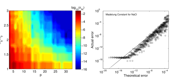
Figure 3: The relative error, $\epsilon_{M}$, in computations of the Madelung constant for NaCl crystal using the present method (colors). The chart on the graph compares the theoretical computational error, $\epsilon_{th}=C_{\epsilon}\left(R_{0}/R_{b}\right)^{p}$ with the actual error for all data points used to plot the chart on the left. Ideally, the graph on the right should be a straight line (shown). Constant $C_{\epsilon}$ was set as $\epsilon_{M}/\epsilon_{th}$ for $p=10$ and $\lambda=R_{b}/R_{0}=1.5$.

Figure 3 shows the dependence of $\epsilon_{M}$ computed for 651 values of parameters $\lambda=R_{b}/R_{0}$ and $p$ controlling the accuracy. The chart on the right shows that the computational errors are consistent with theoretical error bound $\epsilon_{th}=C_{\epsilon}\left(R_{0}/R_{b}\right)^{p}$. For very small values of $\epsilon_{th}$ the computational errors are affected by the double precision roundoff errors. This shows that the parameters can be set to achieve the required accuracy.

Table 1: Error $\epsilon_{M}$ for different check point distributions at $\lambda=R_{b}/R_{0}=\sqrt{3}.$

$p$	Gauss sph. grid	T(256)	T(400)	Rand.$L=2p^{2}$	Rand.$L=3p^{2}$	Rand.$L=5p^{2}$
8	4.85(-6)	3.87(-6)	3.90(-6)	3.39(-5)	2.21(-5)	1.92-(5)
12	1.17(-7)	4.60(-8)	6.28(-8)	1.53(-6)	1.04(-6)	5.10(-7)
16	7.16(-8)	3.43(-7)	2.74(-8)	6.26(-7)	3.50(-7)	1.85(-7)

Table 1 shows some results of the tests with different distributions of the check points. Here for the case of random distributions for any set size we performed 100 runs and the maximum error is reported. It is seen that the lowest errors were achieved using the Thomson point distributions. The number of such points should be not less than $p^{2}-1$, which is necessary (but not sufficient) condition for the use of the present method. When the number of check points approaches $p^{2}-1$ the accuracy of the method deteriorates. Conclusion here is that if a database of the Thomson points or some analogous method of deterministic uniform distribution of the check points exsist, then that method is recommended. In fact, the Gauss spherical grid also provides good results (the order of the error is the same). This grid is easy to generate for any $p$, and that is why this was used in the tests. The error for random distributions is about one order of magnitude larger than that for the Gauss spherical grid or for the Thomson points. It slowly decays with the growing oversampling. Perhaps, there is no reason to use random sets, which anyway show strong dependence of the error on $p$ and also can be used if needed.

We also performed the accuracy test for different basis functions (RBF, Eq. (6)), where 256 Thomson sampling sources $\mathbf{x}_{t}^{(s)}$ were located on ball $S_{b}$, while the check points were the same as for the last line of Table 1 ($p=16$). In this case we obtained $\epsilon_{M}\approx 1.32\cdot 10^{-7}$, which is approximately two times larger than the error when using the spherical basis functions.

4.2 Large scale tests

The large scale tests were conducted for systems with $N$ up to $2^{23}\sim 10^{7}$, for which $O(N\log N)$ summation algorithms are needed. The main purpose of these tests was to check the performance and scaling of the present algorithm. The reported wall clock times were measured on an Intel QX6780 (2.8 GHz) 4 core PC with 8 GB RAM and averaged over ten runs of the same case.

We used a well-tested standard version of the FMM for the Laplacian kernel in three dimensions, where all translations are performed with $O\left(p_{FMM}^{3}\right)$ complexity using the rotation-coaxial translation-back rotation (RCR) algorithm. The code implements a standard multipole-to-local translation stencil with the maximum 189 neighborhood (see details in [40]). The code was parallelized for 4 core CPU machine using OpenMP with parallelization efficiency close to 100%. While faster versions of the FMM were available to the researchers (say utilizing graphics processors, [19]), the version used for the tests was selected to provide consistent scaling of different algorithm parts, as the periodization algorithm was implemented on multicore CPUs. For the tests we treated the FMM as a black box FSA and used it “as is” without any modifications.

First we ran accuracy tests, when the charges have random intensity, $\pm 1$, and zero total sum and are located inside a unit cube at regularly spaced grid points (subgrids of $60\times 60\times 60$ grid). The potential at charge locations (reference solution) was computed with high accuracy using the Ewald method (grid $60\times 60\times 60$, $\xi=15,N_{r}=24$). The present method with $p=40$ and $p_{FMM}=30$ for this case showed error $\epsilon_{2}\approx 1.2\cdot 10^{-10}$. Further performance tests were conducted with lower tolerance to ensure that the error of the reference solution does not affect error and optimization studies. In all cases the Gauss spherical grid ($L=2p^{2}-p$) was used for the check points.

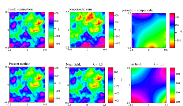
Figure 4: Comparison of periodic solutions at the median plane $z=0$, obtained by different methods for $30\times 30\times 30$ sources of random intensity $q_{i}=\pm 1$ in a unit box. The top row shows respectively the periodic solution obtain by the Ewald method, the non-periodic solution, and the difference between the former and latter potentials. The bottom row shows the periodic solution obtained by the method proposed in this paper, and its near and far field components for $\lambda=1.1$. Computations performed with $p=80,$ $p_{FMM}=16$.

Figure 4 illustrates distribution of potentials generated by 27,000 charges in a box computed by two different methods sampled on $60\times 60\times 60$ grid. It is seen that periodic solutions obtained using the Ewald method and present method are almost the same ($\epsilon_{2}<5\cdot 10^{-7}$), while substantially different from the non-periodic solution (the free field generated by the same sources). This also shows that accounting for the near field (sources in $\Omega_{b}$) substantially improves the non-periodic solution, but the far field component is still of magnitude comparable with the near field. This far field is smooth and its addition to the near field results in an accurate periodic solution.

Table 2: Performance for different $\lambda$ for tolerance $\epsilon_{tol,2}=5\cdot 10^{-7}$ at $N=27,000$, $p_{FMM}=16.$

$\lambda$	$p_{\min}$	$T^{(get)},$s	$T_{(no\_mean)}^{(get)},$s	$T^{(FMM)},$s	$N_{b}$	$N+2L$	$T^{(set)},$s
1.1	80	2.81	2.64	2.03	97,780	52,440	150
1.2	44	1.95	1.73	1.58	126,744	34,656	5.31
1.3	34	2.03	1.78	1.66	161,072	31,556	1.27
1.5	24	2.21	1.77	1.69	247,742	29,256	0.29
1.7	19	2.53	1.98	1.90	360,640	28,406	0.13

As the theory predicts existence of an optimal value of parameter $\lambda$ for a given tolerance we conducted tests to determine this value experimentally. Tables 2 and 3 display the results of these tests. Here we computed potential alone (no gradient computations). The difference between the cases shown in the tables is in the number of charges (27,000 and 216,000, respectively). In these tests $p_{FMM}=16$, which provided the relative $L_{2}$-norm error of the FMM itself smaller than tolerance $\epsilon_{tol,2}$. Since the truncation number $p$ changes discretely, there is the minimal integer $p=p_{\min}$ at which $\epsilon_{2}<\epsilon_{2,tol}$, where $\epsilon_{2}$ is defined by Eq. (41). This $p$ is slightly depends on $N$ and is shown in the tables. The periodization algorithm was executed with this $p.$ The tables also show the number of sources, $N_{b}$, and the total number of evaluation points, $N+2L$. These numbers provide data of the size of the problem solved by the FMM. It is seen that the FMM execution time is a non-monotonic function of $\lambda$, as at the increasing $\lambda$ we have increasing $N_{b}=O\left(N\lambda^{3}\right)$ and decreasing $L\sim 2p_{\min}^{2}$. It is noticeable that despite of substantial change of $N_{b}$ the FMM time does not change significantly. The time of the “set” part of the algorithm increases dramatically at large $p$ (as $p^{6}$). However, for a given $p$ and computational domain the pseudoniverse matrix can be precomputed and stored independently on the number of charges and their distribution. So this should not be considered as a limiting factor. These tests bring us to conclusion that practical optimal $\lambda$ are in the range $\sim 1.2-1.5$. Smaller or larger $\lambda$ can be also used based on particular problems and other issues (e.g. memory complexity).

Table 3: Performance for different $\lambda$ for tolerance $\epsilon_{tol,2}=5\cdot 10^{-7}$ at $N=216,000$, $p_{FMM}=16.$

$\lambda$	$p_{\min}$	$T^{(get)},$s	$T_{(no\_mean)}^{(get)},$s	$T^{(FMM)},$s	$N_{b}$	$N+2L$	$T^{(set)},$s
1.1	80	15.7	14.6	11.5	782,131	241,440	150
1.2	44	12.6	11.2	10.2	1,015,037	223,656	5.31
1.3	34	12.8	11.1	10.3	1,291,247	220,556	1.27
1.5	25	15.0	12.3	11.7	1,983,665	218,450	0.32
1.7	19	18.7	14.7	14.1	2,887,393	217,406	0.13

Effect of the basis functions on the algorithm performance is shown in Table 4. As in the small size tests 256 Thomson points were selected as the centers of the RBFs. Comparison of the performance obtained using the RBFs vs the spherical basis functions, show that the latter choice is beneficial in terms of the accuracy, while the speed is approximately the same. Nonetheless, the errors for both bases are of the same order, while the RBF implementation is slightly simpler.

Table 4: Performance for different basis functions at $\lambda=1.5,$ $p=16$, $p_{FMM}=12.$

$N$	Basis	$\epsilon_{2}$	$T^{(get)},$s	$T_{(no\_mean)}^{(get)},$s	$T^{(set)},$s
27,000	Spherical	1.3(-5)	1.67	1.30	0.08
	RBF	2.6(-5)	1.74	1.35	0.06
216,000	Spherical	1.6(-5)	12.3	9.57	0.08
	RBF	2.6(-5)	12.7	9.95	0.06

Figure 5: Wall clock times of the present algorithm with the FMM as FSA for $\lambda=1.3$, $p=34$ (filled squares), and with brute-force 4 core CPU summation (filled triangles), and Tesla C2050 GPU summation (filled circles), for a periodic system replicating distribution of $N$ random sources in a unit cube (potential and gradient computations, Laplacian kernel in three dimensions). The corresponding empty squares, triangles and circles, connected by a solid line show performance of the particular FSA for the non-periodic problem with the same source distribution in the unit cube and the same truncation number $p_{FMM}=16$. The dashed lines continue the trendlines to indicate performance, if memory resources had not been exceeded. The quadratic scaling of the brute-force summation, and the linear scaling for the FMM are seen. Brute force GPU sums for this case are faster till about $N\simeq 40,000$.

Figure 5 illustrates scaling of the algorithm with the problem size. In this test $N$ sources were distributed randomly in the unit box and both $\phi$ (with zero mean) and $\nabla\phi$ were computed at the source locations. Here only the time for the “get” part is displayed. For comparison we also plotted the wall clock time for solution of the same non-periodic problem, where the FMM with the same $p_{FMM\text{ }}$was used. (The discussion of GPU times is below). While for the non-periodic case the FMM is scaled approximately as $O(N)$ (with some small $N\log N$ addition due to data structures), the present algorithm is scaled sublinearly at small $N$, while it approaches the same scaling as the regular FMM. Qualitatively this can be explained by complexity of the FMM as it used in the present algorithm for periodization (see Eq. (33), where for simplicity two last terms due to generation and evaluation of expansions are neglected). So the ratio of the FMM time in the present algorithm and the FMM for non-periodic problem can be estimated as

$$\frac{T_{FMM}^{(per)}}{T_{FMM}^{(non)}}\sim\sqrt{\frac{A_{gf}}{B_{gf}}\left(1+\frac{2L\left(\lambda\right)}{N}\right)}.$$ (42)

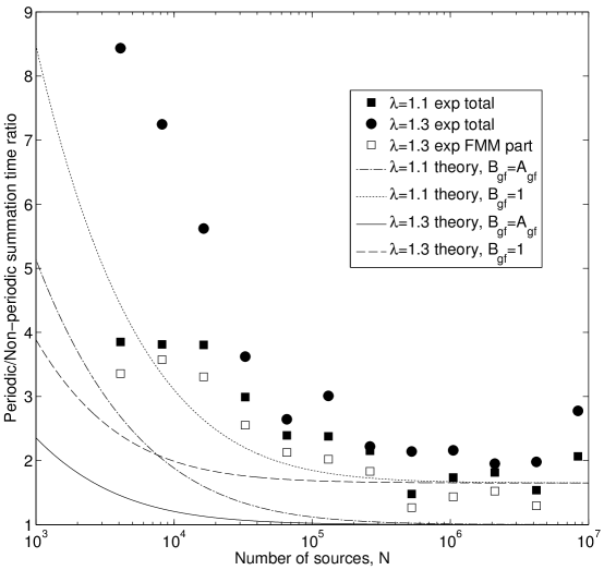
Figure 6: The ratio of the solution times of the periodic and non-periodic problems using the FMM for the cases shown in Fig. 5. Experimental results for the total time for the two cases, and the time taken by the FMM alone for the case $\lambda=1.3$ are shown. Also shown as continuous lines are theoretical estimates via Eq. (42) for the same values, and different geometric factors.

This ratio for different $\lambda$ along with the experimentally measured time ratio of the “get” part of the algorithm and its FMM portion to the FMM for non-periodic problem is plotted in Fig. 6. For each $\lambda$ we presented theoretical ratios (42) computed for limiting cases $B_{gf}=1$ and $B_{gf}=A_{gf}$  (for cubic boxes $A_{gf}\approx 2.72$, see Eq. (32)). It is seen that qualitatively this explains the observed results, and at relatively small $N$ the wall clock time of the present algorithm requires is several times larger than the time of non-periodic FMM. At larger times the ratio should come to an asymptotic limit depending on $\lambda$. Despite Eq. (33) predicts that $\lambda=1.1$ limit should be somehow smaller than $\lambda=1.3$ limit, we found that in the range of experiments they are approximately the same (time ratio about 2, while can be 1.5 or so). The reason why the experimental data deviate from Eq. (42) is that there are some $O(N)$, $O(PN),$ and $O(P^{2})$ overheads in the periodization algorithm. The contribution of these overheads is seen from the difference of the FMM part of the get algorithm and the total cost. We also profiled the FMM, measured performance constants, and found that at large $N\gtrsim 10^{6}$ cost approximation (33) at $B_{gf}=A_{gf}$ is good enough and the FMM part approaches the asymptotic constant, which for cubic domains can be, say, 1.2 ($p_{FMM}=16$).

As the present algorithm can easily treat periodicity for non-cubic domains we conducted accuracy and perfromance tests for periodic boxes of different aspect ratios. The accuracy tests were performed by comparison of the obtained solutions with the results of the Ewald summation in the same way as described above in the range of $N$ from 1000 to 50000. It was found that for fixed $\lambda$ and respective $p\left(\lambda\right)$ the box aspect ratio practically does not affect the accuracy. At large aspect ratios like 5:1:1 we found that conditioning of the system matrix $\mathbf{A}$ (see Eq. (11)) can be poor, but this does not affect the accuracy of the final results and a good algorithm for computing of pseudoinverse can handle that. Some results of performance tests for are shown in Table 5.

Ideally, the time for non-periodic FMM at large $l_{\max}$ should not depend on the box aspect ratio. However, some variation in time is seen, which can be refered to non-perfect (discrete) optimization. For large box aspect ratios one can get $N_{b}$ orders of magnitude larger than $N$ (e.g. two orders for the case 10:1:1). For such cases the cost of computation of the mean, which depends on $N_{b}$ becomes substantial. If these optional computations are not needed, then performance improves, but anyway, solution of periodic problem can be several times more expensive than solution of non-periodic problem. For the cases presented in the table the ratio of these times is well correlated with factor $A_{gf}^{1/2}$. This is consistent with the principal term of the FMM cost (33) at $B_{gf}=1.$

Table 5: Performance for different box aspect ratios at $N=10^{5}$, $\lambda=1.3$, $\ p=34,$ $p_{FMM}=16.$

$d_{1}:d_{2}:d_{3}$	1:1:1	2:1:1	5:1:1	10:1:1	2:2:1	5:5:1	10:2:1
$A_{gf}$	2.72	3.85	14.7	53.9	3.53	7.63	28.2
$N_{b}$	597,625	845,188	3,228,941	11,849,769	776,783	1,675,371	6,192,751
$T^{(get)},$ s	9.08	9.86	20.8	44.5	9.92	13.9	29.8
$T_{(no\_mean)}^{(get)},$ s	8.22	8.77	16.6	29.0	8.92	11.7	21.8
$T_{(no\_mean)}^{(get)}/A_{gf}^{1/2},$ s	4.98	4.47	4.33	3.94	4.74	4.24	4.11
$T_{FMM}^{(non)},$ s	3.76	4.71	4.03	3.40	3.45	5.65	4.79

Finally we note that it is not an easy task to compare the absolute performance of the present methods with the smooth particle mesh Ewald (SPME) and other algorithms for periodic summation due to a difference in implementation, accuracy, what is actually computed (potential and gradient), hardware, etc. However, some comparison with that approaches can be done using published data [17] comparing performance of the SPME and FMM-type PWA implementation for clusters, for relatively small size problems ($N=10^{4}$ and $N=10^{5}$). The absolute figures indicate that the wall clock time of the present algorithm for these sizes is of the same order as the reported times for those methods, while we are able to perform computations with larger problem sizes on relatively modest hardware.

4.3 Using graphics processing units (GPUs) for summation

GPUs are often used to accelerate molecular dynamics simulations where periodization may be required. We implemented the “get” part of the algorithm completely on the GPU. Using “brute-force” summation on the GPU and on a multicore CPU as the FSA, we did the same performance tests as for the FMM, see Fig. 5. The ”set” part can be executed on CPU and transferred to the GPU. All parts of the algorithm are highly parallelizable and so while the scaling of the algorithm is quadratic, it is up to two orders of magnitude faster than the multicore CPU version.

Our tests reveal that at large truncation numbers $p$ (typically $p\gtrsim 30$) single precision GPU computations cannot be used for spherical basis function evaluation due to loss of precision in least-squares solution. Double-precision computations provide accurate results with $L_{2}$-norm relative errors of the order $10^{-13}-10^{-15}$ in potential and gradient computations compared to the double precision CPU computations. Accordingly Fig. 5, only shows double precision times. High performance implementation of the brute-force summation is described in [19] and was used in the present tests with single and double precision, and run on a single NVIDIA Tesla C2050 card. The CPU wall clock times used for comparisons were measured for algorithm parallelized for 4 core PC described before.

Fig. 5 shows the results of tests. It is seen that despite the asymptotic quadratic scaling of the algorithm the GPU implementation can be faster or comparable in speed with the FMM running on CPU at $p_{FMM}=16$ for problems of size $N\lesssim 10^{5}$. The ratio of times for solution of periodic and non-periodic problems for brute force computations at large $N$ tends to theoretical limit $T_{brute}^{(per)}/T_{brute}^{(non)}=\pi\sqrt{\frac{3}{4}}\lambda^{3}$, which for $\lambda=1.3$ used for illustrations is about 6 times. Of course, this ratio can be reduced by decreasing $\lambda$. However, in the range $N\lesssim 10^{5}$ reduction of $\lambda$ below 1.1 does not benefit the overall performance due to increase of the size of the expansion and reduction of the performance of evaluation of the far field on the GPU, where the local memory is substantially smaller than the CPU cache. One of the advantages of brute force double precision GPU computing for problems of relatively small size ($N\lesssim 10^{5}$) is that besides the roundoff errors the accuracy is controlled only by parameters $p$ and $\lambda$, while for the FSA=FMM the error is controlled also by $p_{FMM}$. For efficient FMM implementations on GPU this number is usually small [19] while the efficiency of the FMM on GPU for high accuracy simulations is a subject for a separate study.

5 Discussion

By proposing a method for computation of periodic sums we do not mind to compete with or diminish the role of the existing methods, such as based on Ewald summation or the FMM for periodic functions for well-studied kernels. We realize that a variety of problems with periodic boundary conditions and practical concerns of researchers may require some solutions different from the existing approaches, as any of them, including the present one has some advantages and disadvantages. Such problems are not limited with Laplacian kernels. However, development of specialized approaches which usually are more efficient than generic approaches (kernel-independent FMM is an example), also have some cost and availablity of a method which turns an available FSA to its periodic version without any intervention to the basic FSA algorith, in our opinion, is useful.

The “cons” and “pros” of the FFT vs FMM were discussed in the literature, including performance and scaling at large $N$ (e.g. [22]) and application to solution of molecular dynamics problems (e.g. [41]). Particularly, some difficulties for the use of the FMM for the MD simulations were reported as a long term energy drift was observed in some computations using four or six term expansion in the FMM [42] (perhaps, $p_{FMM}=4$ or $6$, which provides $p_{FMM}^{2}=16$ and 36 terms of expansion, respectively). Of course, the number of terms should be evaluated carefully and the FMM and other errors should be consistent with the integration schemes used (particularly, the FMM errors in gradients are higher than in the potential [39]). In this context, we can mention that in the present algorithm one can enforce some conditions (such as setting the mean of the potential to zero, similarly to the Ewald scheme), which is normally is not controlled in the FMM-based algorithms. It can be more stable or not in terms of the energy drift if applied to the MD simulations, but this requires an additional study, which, certainly, goes beyond the scope of the present work, where not only the MD applications are envisioned. Another advantage of not requiring the FFT may arise for very large problems, which have to be implemented on distributed architectures, where the communication costs of the FMM are smaller than the FFT.

As far as comparing the present approach with an FMM algorithm implemented using periodic kernel functions is considered, we perform this comparison on three sizes of problems: with small $N\$(say, $N\lesssim 10^{3}$), moderate $N$ (say, $10^{4}\lesssim N\lesssim 10^{5}$) and large $N$ (say, $N\gtrsim 10^{6}$). The first class may not require the FMM at all, as direct sums may be done faster and be more accurate, and the present algorithm can work efficiently and accurately (choosing proper $p$) with direct sums. The second and the third types of the problems require a fast summation algorithm such as the FMM. In this case some authors claim that the overheads for solution of periodic problems are negligibly small compared to solution of the non-periodic problem. For example, Ref. [12] claims that periodization of requires only 0.1% of the total computational time. This statement does not mean that the periodic version of the sum is 1.001 times slower than the solution of the non-periodic sum, as was remarked on an early draft of this paper. Indeed, in [12] (page 1084 and Table V) it is stated “The time spent on dealing with periodicity ranged from about 0.3 to 2.6 times of that of the free boundary computations, depending on the values of $p$ and $L$ and the type of the FMM.” (Here $L=l_{\max}$ in our notation). This shows that actual measured time ratios, such as reported in Fig. 6, were in the range 1.3 to 3.6.

The overhead comes from the fact that the periodic FMM is the FMM executed in the extended domain, which is not the original cell $\Omega_{0}$, but in $\Omega_{0}$ with its 26 neighbors, which is $\Omega_{b}$ in our notation, see Fig. 1. The difference between the present and periodic FMMs is that, first, the periodic FMM saves on generation of multipole expansions and multipole-to-multipole translations for the replicated domains, which is not implemented in the present algorithm, and, second, that for the present FMM some relatively small amount of receivers (“check points”) are added. Discussions of the FMM costs and simplifications in Appendix A and around Eqs (33) and (42) show that asymptotically as $N\rightarrow\infty$ the second modification brings a negligible overhead, while the overhead due to the first modification is non-zero, and in practice can be several percents for cubic $\Omega_{0}$ to tens of percents for non-cubic $\Omega_{0}$ (due to the geometric factor $A_{gf}$ ), which is the price of use of the FMM as a black box FSA.

At $N\rightarrow\infty$ the costs of the periodic and non-periodic FMMs are the same. The difference in costs of periodic and non-periodic FMMs comes from two factors – the difference in the multipole-to-local translations and direct summations for the boxes near the boundaries of $\Omega_{0}$, due to the difference in the neighborhoods. We carefully counted these numbers accounting for the boundary effects, and found that for levels $l_{\max}=3$ and $4$ (midsize problems) used in [12], the ratios of numbers of translations in periodic and non-periodic FMMs is 1.96 and 1.38, while the ratios of the numbers of direct summations is 1.30 and 1.14, respectively. At levels $l_{\max}=5$ and $6$ one can expect time ratios in a range 1.05-1.20.

One of the features of the present algorithm, which may be of practical interest, is the capability to obtain periodic solutions for non-cubic domains easily, which can be an issue for some other algorithms. These were illustrated in Table 5. Performance for moderate box aspect ratio is comparable to the cubic case. For high aspect ratios, the algorithm works, but some issues, which could be the subject of future study must be noted. There is a substantial increase in the amount of sources added because of the enclosure of the whole domain in a sphere. Because of this, both the memory needed and the computational time are relatively large, while still scaled as expected. Possible ways to address this would be to devise more check point sets located not on a sphere, but on surface that are more conformal to the boundaries, and also a reduction of the size of domain $\Omega_{0}$. The latter can be achieved in a few ways including distribution of RBF centers not too far from the boundaries of $\Omega_{0}$ or to use basis functions, which are better suited for boxes of high aspect ratios than the spherical basis functions.

6 Conclusion

We have presented a kernel-independent method for the periodization of finite sums. The technique was presented in a general setting, and then applied to the particular case of the Laplacian kernel using different expansion bases. Tests showed that the method can be tuned to compute periodic sums with arbitrary prescribed accuracy. In the case of use of the FMM as the fast summation algorithm the complexity of the method at large $N$ is the same as the FMM. The computational time for large $N$ (in tests up to $N=2^{23}$) is about twice that for the finite box sum using the FMM. Similar results are seen for GPU based FSA, though here the scaling is quadratic, and the largest problem size that can be reasonably treated is about $10^{5}$. The ease of implementation of the periodization method, its performance, and capability to “retrofit” any available black box FSA without any modification makes it practical. This method may also be valuable on distributed architectures on which communication costs of an algorithm are as important as computational complexity. FMM-based approaches are known to be much more communication efficient than FFT-based approaches for solution of the same large problems on distributed architectures. Additional speedups of the method can be achieved by specialization of the FMM – these were specifically avoided in this paper to demonstrate the ability to use a blackbox sum algorithm, and should be investigated if the method is to be used in a “production” environment. Application to other kernels should be straightforward, though details will have to be worked out for them.

Appendix A Complexity of the FMM

There are many papers evaluating complexity of the FMM in basic settings (mostly for the cases when the sources and receivers are the same and uniformly occupy all computational domain, which can be thougth as a unit cubic box, e.g. [40]). Here, we consider the FMM for Laplace-like kernels and modify the problem by assuming that $N_{b}$ sources are located in the domain $\Omega_{b}$ of volume $V_{b}$ and $M$ receivers are distributed inside the domain $\Omega_{r}\subset\Omega_{b}$ of volume $V_{r}.$ Let now $U$ be a minimal cube which includes $\Omega_{b}$ and presents the zero level of the octree. The cube is partitioned via the octree down to level $l_{\max}$, in which case the maximum number of sources in a box is $s$. Assuming more or less uniform source point distribution in $\Omega_{b}$ and that any box in $\Omega_{r}$ contains at least one receiver point, we can determine the number of source and receiver boxes at this level as $B_{s}=N_{b}/s$ and $B_{r}=B_{s}V_{r}/V_{s}$, respectively. The latter estimate comes from the observation that for large enough $l_{\max}$ the ratio of the numbers of source and receiver boxes is approximately the same as the ratio of volumes of the domains occupied by the sources and receivers. In a standard FMM in three dimensions the number of multipole-to-local translations to each receiver box located far enough from the boundary of $\Omega_{b}$ is $K=189$ (this number can be reduced, e.g. as in [19], but anyway, $K\gg 1$). When counting the total number of translations $K$ should be increased to account for one local-to-local transaltion per receiver box and 1 multipole-to-multipole translation per source box. It can be noted then that the amount of translations at the $l$th level of the octree increases geometrically with the level (8 times in three dimensions), so the total number of translations, $N_{trans}$, will have factor $8/7$ compared to the number of translations at level $l_{\max}$ and we have

$$N_{trans}\sim\frac{8}{7}\left(B_{s}+KB_{r}\right)=\frac{8N_{b}}{7s}\left(1+K\frac{V_{r}}{V_{s}}\right)\approx\frac{8N_{b}}{7s}\frac{KV_{r}}{V_{s}}.$$ (43)

Here the latter approximate equality holds when $K\gg V_{s}/V_{r}$. The number of direct summations per receiver is 27$s$, if we assume that the neighborhood of the receiever box consists of 27 boxes, which yields the total number of direct summations, $N_{dir}=27Ms.$ Hence, denoting $C_{trans}$ the cost of a single translation and $C_{dir}$ the cost of a single direct evaluation, we obtain the part of the total cost, which depends on $s$ in the form

$$C_{s}=\frac{8N_{b}}{7s}\frac{KV_{r}}{V_{s}}C_{trans}+27sMC_{dir}.$$ (44)

This function can be minimized with respect to $s$, and the minimum cost denoted as, $C_{s,\min}$, at $s=s_{opt}$, where from $dC_{s}/ds=0$, we have

$$s_{opt}=\sqrt{\frac{8KC_{trans}}{189C_{dir}}\frac{N_{b}}{M}\frac{V_{r}}{V_{s}}},\quad C_{s,\min}=C_{td}\sqrt{MN_{b}\frac{V_{r}}{V_{s}}},\quad C_{td}=4\sqrt{\frac{54K}{7}C_{trans}C_{dir}}$$ (45)

To get the total cost of the FMM, we need to add here the cost of generation of multipole expansions, $C_{gen}N_{b}$ and the cost of evaluation of local expansions, $C_{ev}M$, where $C_{gen}$ and $C_{ev}$ are the costs of generation and evaluation of single expansions, which does not depend on $s$, or the depth of hte octree $l_{\max}$. Hence, the total cost of the FMM used in the present algorithm, which neglects the cost of generation of data structure is

$$C^{(FMM)}=C_{td}\sqrt{MN_{b}\frac{V_{r}}{V_{s}}}+C_{gen}N_{b}+C_{ev}M.$$ (46)

Here the last estimate comes from the fact that usually translations and direct summations are the major contributors to the overall cost of the FMM (e.g. see profiling of the algorithm [19]). Also note the dependence of the FMM cost on the number of terms in the multipole and local expansions used in the FMM, $P_{FMM}$. We have $C_{gen}\sim C_{gen}=O\left(P_{FMM}\right)$, $C_{trans}=O\left(P_{FMM}^{\alpha}\right),$ and $C_{td}=O\left(P_{FMM}^{\alpha/2}\right)$ where $\alpha$ is some number (e.g. for $O\left(p^{3}\right)$ translation methods, $\alpha=3/2$).

Appendix B Box integrals of the basis functions

Basis functions $R_{n}^{m}\left(\mathbf{y}\right)$ are homogeneous polynomials of degree $n$ (sums of monomials $x^{n_{1}}y^{n_{2}}z^{n_{3}},$ $n_{1}+n_{2}+n_{3}=1$). We can compute the integrals as

$$R_{t}^{(0)} = \frac{1}{V_{0}}\int_{\Omega_{0}}R_{t}\left(\mathbf{y}\right)dV\left(\mathbf{y}\right)=\frac{1}{d_{1}d_{2}d_{3}}\int_{-d_{1}/2}^{d_{1}/2}\int_{-d_{2}/2}^{d_{2}/2}\int_{-d_{3}/2}^{d_{3}/2}R_{t}\left(x,y,z\right)dxdydz$$

$$= \frac{1}{8}\sum_{i=1}^{N_{q}}\sum_{j=1}^{N_{q}}\sum_{k=1}^{N_{q}}w_{i}w_{j}w_{k}R_{t}\left(\frac{1}{2}d_{1}x_{i},\frac{1}{2}d_{2}x_{j},\frac{1}{2}d_{3}x_{k}\right),$$

where $w_{i}$ and $x_{i}$ are the standard weights and abscissas of the Gauss quadrature of order $N_{q}$ [33]. Since this integration is exact for polynomials of degree $n<2N_{q}$ and the maximum degree of the polynomials in the sum is $p-1,$ the choice

$$N_{q}=\left[\frac{p-1}{2}\right]+1,\quad p=P^{1/2},$$ (48)

provides an exact result. For evaluation of all $P$ required coefficients $\widehat{R}_{n}^{m(0)}$ the computational cost of this procedure is $O\left(P^{5/2}\right).$ Note that faster methods may be proposed for computation of this step. However, this is not crucial, as this integration is performed in the “set” part of the algorithm, which overall cost is $O\left(P^{3}\right)$, and this cost is amortized over the rest of the algorithm.

Appendix C Mean computations

To compute the integral (39) for the kernel (2), we first apply the Gauss divergence theorem to reduce the volume integral to a surface integral:

$$\Phi_{0}\left(\mathbf{x}\right)=\frac{1}{V_{0}}\int_{\Omega_{0}}\frac{dV\left(\mathbf{y}\right)}{\left|\mathbf{y}-\mathbf{x}\right|}=\frac{1}{2V_{0}}\int_{\Omega_{0}}\nabla_{\mathbf{y}}\cdot\left(\frac{\mathbf{y}-\mathbf{x}}{\left|\mathbf{y}-\mathbf{x}\right|}\right)dV\left(\mathbf{y}\right)=\frac{1}{2V_{0}}\int_{\partial\Omega_{0}}\frac{\mathbf{n}\cdot\left(\mathbf{y}-\mathbf{x}\right)}{\left|\mathbf{y}-\mathbf{x}\right|}dS\left(\mathbf{y}\right),$$ (49)

where $\mathbf{n}$ is the outward normal to $\Omega_{0}.$ This result is valid for an arbitrary point $\mathbf{x}$ including when $\mathbf{x}$ is located in $\Omega_{0}$ or on its boundary $\partial\Omega_{0}$. This can be checked by consideration of $\epsilon$-vicinities of singularities, which are integrable. The surface integral can be decomposed into integrals over the box faces, $S_{k}$, $k=1,...,6.$

$$\Phi_{0}\left(\mathbf{x}\right) = \frac{1}{2V_{0}}\sum_{k=1}^{6}\int_{S_{k}}\frac{\mathbf{n}_{k}\cdot\left(\mathbf{y}-\mathbf{x}\right)}{\left|\mathbf{y}-\mathbf{x}\right|}dS\left(\mathbf{y}\right)=-\frac{1}{2V_{0}}\sum_{k=1}^{6}\left(\mathbf{n}_{k}\cdot\mathbf{x}_{k}\right)L_{k}\left(\mathbf{x}_{k}\right),\quad$$ (50)

$$L_{k}\left(\mathbf{x}_{k}\right) = \int_{S_{k}}\frac{dS\left(\mathbf{y}_{k}\right)}{\left|\mathbf{y}_{k}-\mathbf{x}_{k}\right|},\quad\mathbf{y}_{k}=\mathbf{y-y}_{k0},\quad\mathbf{x}_{k}=\mathbf{x-y}_{k0},$$

where $\mathbf{n}_{k}$ and $\mathbf{y}_{k0}$ are the normal and the center of the $k$th face, while $\mathbf{y}_{k}$ and $\mathbf{x}_{k}$ are coordinates in the reference frame with the origin at the $k$th face center. The surface integral then can be reduced to the contour integral using, e.g. the Gauss divergence theorem in the plane of a particular face. Indeed, consider function

$$\mathbf{F}_{k}\left(\mathbf{r}_{k}\right) = \mathbf{r}_{k}f_{k}\left(r_{k};h_{k}\right),\quad f_{k}\left(r_{k};h_{k}\right)=\frac{\rho_{k}-h_{k}}{r_{k}^{2}},\quad\rho_{k}=\sqrt{r_{k}^{2}+h_{k}^{2}}\left(=\left|\mathbf{y}_{k}-\mathbf{x}_{k}\right|\right),\quad$$ (51)

$$\quad\mathbf{r}_{k} = \mathbf{y}_{k}-\mathbf{x}_{k}^{\prime},\quad\mathbf{x}_{k}^{\prime}=\mathbf{x}_{k}-\mathbf{n}_{k}h_{k},\quad h_{k}=\mathbf{n}_{k}\cdot\mathbf{x}_{k}.$$

The 2D divergence of this function in the plane of the $k$th face is $1/\rho_{k}$. So

$$L_{k}\left(\mathbf{x}_{k}\right)=\int_{S_{k}}\widetilde{\nabla}_{\mathbf{r}_{k}}\cdot\mathbf{F}_{k}\left(\mathbf{r}_{k}\right)dS\left(\mathbf{r}_{k}\right)=\int_{C_{k}}\mathbf{n}_{k}^{\prime}\cdot\mathbf{F}_{k}\left(\mathbf{r}_{k}\right)dl\left(\mathbf{r}_{k}\right),$$ (52)

where $\mathbf{n}_{k}^{\prime}$ is the outer normal to the contour $C_{k}=\partial\Omega_{k}$. This integral can be decomposed into four integrals over the face edges. So

$$L_{k}\left(\mathbf{x}_{k}\right)=\sum_{j=1}^{4}I_{kj}\left(\mathbf{x}_{k}\right),\quad I_{kj}\left(\mathbf{x}_{k}\right)=\int_{C_{kj}}\mathbf{n}_{kj}^{\prime}\cdot\mathbf{r}_{k}\frac{\rho_{k}-h_{k}}{r_{k}^{2}}dl.$$ (53)

The latter integrals can be found analytically. Indeed, consider for the $j$th edge a local right hand oriented reference frame centered at its endpoint $\mathbf{y}_{kj0}$ from which integration starts, and unit basis vectors $\mathbf{i}_{kjx}^{\prime}$ directed along the integration path, $\mathbf{i}_{kjy}^{\prime}=\mathbf{n}_{k}$ and $\mathbf{i}_{kjz}^{\prime}=\mathbf{n}_{kj}^{\prime}=\mathbf{i}_{kjx}^{\prime}\times\mathbf{i}_{kjy}^{\prime}.$ Denoting coordinates of $\mathbf{x}$ in this reference frame as

$$x_{kj}=\left(\mathbf{x}_{k}-\mathbf{y}_{kj0}\right)\cdot\mathbf{i}_{kjx}^{\prime},\quad y_{kj}=\left(\mathbf{x}_{k}-\mathbf{y}_{kj0}\right)\cdot\mathbf{i}_{kjy}^{\prime},\quad z_{kj}=\left(\mathbf{x}_{k}-\mathbf{y}_{kj0}\right)\cdot\mathbf{i}_{kjz}^{\prime},$$ (54)

we obtain

$$I_{kj}\left(\mathbf{x}_{k}\right)=-z_{kj}\int_{-x_{kj}}^{l_{kj}-x_{kj}}f\left(r_{kj};\left|y_{kj}\right|\right)dx=H\left(l_{kj}-x_{kj},\left|y_{kj}\right|,z_{kj}\right)-H\left(-x_{kj},\left|y_{kj}\right|,z_{kj}\right),$$ (55)

where $r_{kj}^{2}=x^{2}+z_{kj}^{2}$, $l_{kj}$ is the length of edge $C_{kj}$, and $H\left(x,y,z\right)$ is the primitive,

$$H\left(x,y,z\right)=-z\int f\left(r;\left|y\right|\right)dx,\quad f\left(r;y\right)=\frac{\rho-\left|y\right|}{r^{2}},\quad r^{2}=x^{2}+z^{2},\quad\rho=\sqrt{r^{2}+y^{2}},$$ (56)

which can be computed analytically as

$$H\left(x,y,z\right)=\left|y\right|\left(\arctan\frac{x}{z}-\arctan\frac{\left|y\right|x}{z\rho}\right)-z\ln\left|\rho+x\right|+C\left(y,z\right).$$ (57)

The integration constant $C\left(y,z\right)$ can be selected arbitrarily to eliminate possible singularities. Particularly for $y\neq 0,$ $z=0$ one can set $H=0$. The above formulae are sufficient for numerical implementation, which in the simplest form can program the primitive (57) and implement the above decompositions. There exist some box symmetries (e.g. all local coordinates are nothing but permuted and shifted original Cartesian coordinates), which can be exploited to achieve better performance.

Appendix D Ewald summation

The Ewald summation method is based on decomposition of kernel (2)

$$K\left(\mathbf{y}-\mathbf{x}\right) = K_{1}\left(\mathbf{y}-\mathbf{x};\;\xi\right)+K_{2}\left(\mathbf{y}-\mathbf{x};\;\xi\right),\quad$$ (58)

$$K_{1}\left(\mathbf{y}-\mathbf{x};\;\xi\right) = \frac{\text{erfc}\left(\xi\left|\mathbf{y}-\mathbf{x}\right|\right)}{\left|\mathbf{y}-\mathbf{x}\right|},\quad\mathbf{y}\neq\mathbf{x;\quad}K_{1}\left(\mathbf{0};\;\xi\right)=-\frac{2\xi}{\sqrt{\pi}},$$

$$K_{2}\left(\mathbf{y}-\mathbf{x};\;\xi\right) = \frac{\text{erf}\left(\xi\left|\mathbf{y}-\mathbf{x}\right|\right)}{\left|\mathbf{y}-\mathbf{x}\right|},\quad\forall\mathbf{y},\mathbf{x}\in\mathbb{R}^{3},\quad\left(K_{2}\left(\mathbf{0};\;\xi\right)=\frac{2\xi}{\sqrt{\pi}}\right),$$

which is exact for any value of parameter $\xi$, since by definition of the error function, erf$\left(x\right)$, and the complimentary error function, erfc$\left(x\right)$, we have erf$\left(x\right)+$erfc$\left(x\right)=1$ and the value of $K_{1}\left(\mathbf{0;}\xi\right)$ is set due to by definition $K\left(\mathbf{0}\right)=0.$ So for the total potential (2) we have

$$\phi\left(\mathbf{y}\right) = \phi_{1}\left(\mathbf{y}\right)+\phi_{2}\left(\mathbf{y}\right),\quad\phi_{1}\left(\mathbf{y}\right)=\sum_{\mathbf{p}}\sum_{i=1}^{N}q_{i}K_{1}\left(\mathbf{y}-\mathbf{x}_{i}+\mathbf{p};\;\xi\right),$$

$$\phi_{2}\left(\mathbf{y}\right) = \sum_{\mathbf{p}}\sum_{i=1}^{N}q_{i}K_{2}\left(\mathbf{y}-\mathbf{x}_{i}+\mathbf{p};\;\xi\right).$$ (59)

Both functions $\phi_{1}\left(\mathbf{y}\right)$ and $\phi_{2}\left(\mathbf{y}\right)$ are periodic.

Due to fast decay of erfc$\left(x\right)$ computation of $\phi_{1}\left(\mathbf{y}\right)$ for $\mathbf{y}\in\Omega_{0}$ can be done only using the sources in some neighborhood of $\Omega_{0}$, namely in $\Omega_{1}\supset\Omega_{0}$ such that the minimum distance, $a$, between the points on the boundaries $\partial\Omega_{0}$ and $\partial\Omega_{1}$ is much larger than $1/\xi$. Hence, this can be computed directly by evaluation of a finite sum with a controllable error as

$$\phi_{1}\left(\mathbf{y}\right)=\sum_{\mathbf{x}_{j}\in\Omega_{1}\left(\xi\right)}q_{j}K_{1}\left(\mathbf{y}-\mathbf{x}_{j};\;\xi\right)+O\left(e^{-\xi^{2}a^{2}}\right).$$ (60)

For computation of $\phi_{2}\left(\mathbf{y}\right)$ one can notice that $K_{2}$ is a solution of the Poisson equation

$$\nabla^{2}K_{2}\left(\mathbf{y}-\mathbf{x};\;\xi\right)=-4\pi\delta_{\xi}\left(\mathbf{y}-\mathbf{x}\right),\quad\delta_{\xi}\left(\mathbf{y}-\mathbf{x}\right)=\frac{\xi^{3}}{\pi^{3/2}}e^{-\xi^{2}\left|\mathbf{y}-\mathbf{x}\right|^{2}},$$ (61)

where $\delta_{\xi}\left(\mathbf{y}-\mathbf{x}\right)$ is a compactly supported function, which turns to the Dirac delta-function as $\xi\rightarrow\infty$. Periodic solution of the Poisson equation can be obtained via the FFT. For this purpose, we grid the domain $\Omega_{0}$ and select $\xi$ in a way that $\xi\ll 1/h$, and $\xi\gg 1/\max\left(d_{1},d_{2},d_{3}\right)$ (an optimal setting can be found from analysis of the error bounds), where $h$ is the minimum spatial step of the grid. This enables sampling of $\delta_{\xi}\left(\mathbf{y}-\mathbf{x}\right)$ for source $\mathbf{x=x}_{i}$ at several grid points around $\mathbf{x}_{i}$. The number of these grid points determines the accuracy of the method (at optimal settings), so we introduce additional parameter $N_{r}$, so $\delta_{\xi}\left(\mathbf{y}\right)$ is sampled in a box $\left(2N_{r}+1\right)\times\left(2N_{r}+1\right)\times(2N_{r}+1)$. We also take care about the points $\mathbf{x}_{i}$ located near the boundary of $\Omega_{0}$ by periodization (so we construct a periodic function $\delta_{\xi}^{(\mathbf{p})}\left(\mathbf{y}-\mathbf{x}\right)$). Further, we apply the forward 3D FFT to

$$f_{2}\left(\mathbf{y}\right)=\nabla^{2}\phi_{2}\left(\mathbf{y}\right)=-4\pi\sum_{i=1}^{N}q_{i}\delta_{\xi}^{(\mathbf{p})}\left(\mathbf{y}-\mathbf{x}_{i}\right),$$ (62)

and zero the harmonic of the Fourier image $f_{2}^{\ast}\left(\mathbf{k}\right)$ corresponding to the wavenumber $k=0.$ The inverse 3D FFT of $\phi_{2}^{\ast}\left(\mathbf{k}\right)=-k^{-2}f_{2}^{\ast}\left(\mathbf{k}\right)$, produces the required solution $\phi_{2}\left(\mathbf{y}\right)$ with zero mean at grid points. Note then that solution obtained in this way has the following mean

$$\phi_{mean}\left(\xi\right)=\left\langle\phi\left(\mathbf{y}\right)\right\rangle_{\Omega_{0}}=\frac{1}{V_{0}}\sum_{\mathbf{x}_{j}\in\Omega_{1}\left(\xi\right)}q_{j}\int_{\Omega_{0}}K_{1}\left(\mathbf{y}-\mathbf{x}_{j}\mathbf{;}\xi\right)dV\approx 0.$$ (63)

The zero mean here is due to the compact support of the kernel $K_{1}$ and charge neutrality. This mean can be computed using decomposition $K_{1}\left(\mathbf{y}-\mathbf{x}_{j}\mathbf{;}\xi\right)=K\left(\mathbf{y}-\mathbf{x}_{j};\xi\right)-K_{2}\left(\mathbf{y}-\mathbf{x}_{j};\xi\right)$, where the integral with the first kernel can be computed analytically (see Appendix C), while the integral with the second kernel is regular and can be computed using, say, the trapezoidal rule (in the FFT-based method the space is gridded). To avoid interpolation errors, in the numerical tests where we compared our method for accuracy with the Ewald summation method, we used only cases when the source and evaluation points are located at the grid nodes.

References

- [1] P. Ewald, Die Berechnung optischer und elektrostatischer Gitterpotentiale, Ann. Phys. 369 (1921) 253-287.
- [2] T. Darden, D. York, and L. Pedersen, Particle mesh Ewald - an Nlog(N) method for Ewald sums in large systems, J. Chem. Phys. 98 (1993) 10089-10092.
- [3] U. Essmann, L. Perera, M.L. Berkowitz, T. Darden, H. Lee, and L.G. Pedersen, A smooth particle mesh Ewald method, J. Chem. Phys. 103 (1995) 8577-8593.
- [4] D. Lindbo and A.-K. Tornberg, Spectrally accurate fast summation for periodic Stokes potentials, J. Comput. Phys. 229 (2010) 8994-9010.
- [5] D. Lindbo and A.-K. Tornberg, Spectral accuracy in fast Ewald-based method for particle simulations, J. Comput. Phys. 230 (2011) 8744-8761.
- [6] L. Greengard and V. Rokhlin, A fast algorithm for particle simulations, J. Comput. Phys. 73 (1987) 325-348.
- [7] K.E. Schmidt and M.A. Lee, Implementing the fast multipole method in three dimensions, J. Stat. Phys. 63 (1991) 1223-1235.
- [8] D. Christiansen, J.W. Perram, and H.G. Petersen, On the fast multipole method for computing the energy of periodic assemblies of charged and dipolar particles, J. Comput. Phys. 107 (1993) 403-405.
- [9] J.T. Hamilton and G. Majda, On the Rokhlin-Greengard method with vortex blobs for problems posed in all space or periodic in one direction, J. Comput. Phys 121 (1995) 29-50.
- [10] C.G. Lambert, T.A. Darden, and J.A. Board, Jr., A multipole-based algorithm for efficient calculation of forces and potentials in macroscopic periodic assemblies of particles, J. Comput. Phys. 126 (1996) 274-285.
- [11] F. Figueirido, R.M. Levy, R. Zhou, and B.J. Berne, Large scale simulation of macromolecules in solution: Combining the periodic fast multipole method with multiple step integrators, J. Chem. Phys. 106 (1997) 9835-9849.
- [12] T. Amisaki, Precise and efficient Ewald summation for periodic fast multipole method, J. Comput. Chemistry 21 (2000) 1075-1087.
- [13] Y. Otani and N. Nishimura, A fast multipole boundary integral equation method for periodic boundary value problems in three-dimensional elastostatics and its application to homogenization, Int. J. Multiscale Computational Eng. 4 (2006) 487-500.
- [14] Y. Otani and N. Nishimura, A periodic FMM for Maxwell’s equations in 3D and its application to problems related to photonic crystals, J. Comput. Phys. 227 (2008) 4630-4652.
- [15] A. Barnett and L. Greengard, A new integral representation for quasi-periodic fields and its application to two-dimensional band structure calculations, J. Comput. Phys 229 (2010) 6898-6914.
- [16] M.H. Langston, L. Greengard, and D. Zorin, A free-space adaptive FMM-based PDE solver in three dimensions, Comm. Appl Math and Comput. Sci. 6 (2011) 79-122.
- [17] A. Kia, D. Kim, and E. Darve, Fast electrostatic force calculation on parallel computer clusters, J. Comput. Phys 227 (2008) 8551-8567.
- [18] J.E. Stone, J.C. Phillips, P.L. Freddolino, D.J. Hardy, L.G. Trabuco, and K. Schulten. Accelerating molecular modeling applications with graphics processors. J. Comput. Chem., 28 (2007) 2618-2640.
- [19] N.A. Gumerov and R. Duraiswami, Fast multipole methods on graphics processors, J. Comput. Phys. 227 (2008) 8290-8313.
- [20] T. Hamada, R. Yakota, K. Nitadori, T. Narumi, K. Yasuoka, and M. Taiji, 42 TFlops hierarchical N-body simulations on GPUs with applications in both astrophysics and turbulence, Proceedings of International Conference for High Performance Computing, Networking, Storage, and Analysis, ser. SC’09. New York, NY:ACM, 2009, Article No. 62.
- [21] Q. Hu, N.A. Gumerov, and R. Duraiswami, Scalable fast multipole methods on distributed heterogeneous architectures, Proceedings of International Conference for High Performance Computing, Networking, Storage, and Analysis, ser. SC’11. New York, NY:ACM, 2011, pp. 36:1–36:12.
- [22] R. Yokota, L.A. Barba, T. Narumi, and K. Yasuoka, Petascale turbulence simulation using a highly parallel fast multipole method on GPUs, Computer Phys. Communications 184 (2013) 445-455.
- [23] N.A. Gumerov and R. Duraiswami, Fast multipole method for the biharmonic equation in three dimensions, J. Comput. Phys. 215 (2006) 363-383.
- [24] M. Buhmann, Radial Basis Functions: Theory and Implementations, Cambridge, 2003.
- [25] Z. Gimbutas and V. Rokhlin, A generalized fast multipole method for nonoscillatory kernels, SIAM J. Sci. Comput. 24 (2003) 796-817.
- [26] L. Ying, G. Biros, and D. Zorin, A kernel-independent adaptive fast multipole algorithm in two and three dimensions, J. Comput. Phys. 196 (2004) 591-626.
- [27] L. Ying, A kernel independent fast multipole algorithm for radial basis functions, J. Comput. Phys. 213 (2006) 451-457.
- [28] A. Barnett and L. Greengard, A new integral representation for quasi-periodic scattering problems in two dimensions, BIT Numer. Math. 51 (2011) 67-90.
- [29] W. Fong and E. Darve, The black-box fast multipole method, J. Comput. Phys. 228 (2009) 8712-9725.
- [30] B. Zhang, J. Huang, N.P. Pitsianis, and X. Sun, A Fourier-series-based kernel independent fast multipole method, J. Comput. Phys. 230 (2011) 5807-5821.
- [31] M. Messner, M. Schanz, and E. Darve, Fast directional multilevel summation for oscillatory kernels based on Chebyshev interpolation, J. Comput. Phys. 231 (2012) 1175-1196.
- [32] G.H. Golub and C.F. Van Loan, Matrix Computations, 3rd edition, John Hopkins University Press, Baltimore, 1996.
- [33] M. Abramowitz and I.A. Stegun, Handbook of Mathematical Functions, National Bureau of Standards, Washington, D.C., 1964.
- [34] J. J. Thomson, On the structure of the atom: an investigation of the stability and periods of oscillation of a number of corpuscles arranged at equal intervals around the circumference of a circle; with application of the results to the theory of atomic structure, Phil. Mag. 7 (1904), 237-265.
- [35] J. Fliege and U. Maier, The distribution of points on the sphere and corresponding cubature formulae, IMA J. Numer. Analysis 19 (1999) 317-334 (data available at http://www.personal.soton.ac.uk/jf1w07/nodes/nodes.html ).
- [36] N.A. Gumerov and R. Duraiswami, Fast Multipole Methods for the Helmholtz Equation in Three Dimensions, Elsevier, Oxford, 2005.
- [37] M.A. Epton and B. Dembart, Multipole translation theory for the three-dimensional Laplace and Helmholtz equations, SIAM J. Sci. Comput., 16 (1995) 865-897.
- [38] E. Madelung, Das elektrische Feld in Systemen von regelmäßig angeordneten Punktladungen. Phys. Zs,, XIX (1918) 524-533.
- [39] N.A. Gumerov and R. Duraiswami, Efficient FMM accelerated vortex methods in three dimensions via the Lamb-Helmholtz decomposition, J. Comput. Phys. 240 (2013) 310-328.
- [40] N.A. Gumerov and R. Duraiswami, Comparison of the efficiency of translation operators used in the fast multipole method for the 3D Laplace equation, Technical Report CS-TR 4701 and UMIACS-TR 2005-09, University of Maryland Department of Computer Science and Institute for Advanced Computer Studies, College Park, November 2005.
- [41] R.D. Skeel, Fast N-body methods: why, what, and which, Proceedings of International Conference on Numerical Analysis and Applied Mathematics, ICNAAM, CP1281, I, (2010) (AIP Conference Proceedings 1281, 27 (2010); doi: 10.1063/1.3498450).
- [42] T.C.Bishop, R.D. Skeel, and K. Schulten, Difficulties with multiple time stepping and fast multipole algorithm in molecular dynamics, J. Comput. Chem. 18 (1997) 1785-1791.