Quantum Monte Carlo methods for nuclear physics
Abstract
Quantum Monte Carlo methods have proved very valuable to study the structure and reactions of light nuclei and nucleonic matter starting from realistic nuclear interactions and currents. These ab-initio calculations reproduce many low-lying states, moments and transitions in light nuclei, and simultaneously predict many properties of light nuclei and neutron matter over a rather wide range of energy and momenta. We review the nuclear interactions and currents, and describe the continuum Quantum Monte Carlo methods used in nuclear physics. These methods are similar to those used in condensed matter and electronic structure but naturally include spin-isospin, tensor, spin-orbit, and three-body interactions. We present a variety of results including the low-lying spectra of light nuclei, nuclear form factors, and transition matrix elements. We also describe low-energy scattering techniques, studies of the electroweak response of nuclei relevant in electron and neutrino scattering, and the properties of dense nucleonic matter as found in neutron stars. A coherent picture of nuclear structure and dynamics emerges based upon rather simple but realistic interactions and currents.
I INTRODUCTION
Nuclei are fascinating few- and many-body quantum systems, ranging in size from the lightest nuclei formed in the big bang to the structure of neutron stars with 10 km radii. Understanding their structure and dynamics starting from realistic interactions among nucleons has been a long-standing goal of nuclear physics. The nuclear quantum many-body problem contains many features present in other areas such as condensed matter physics, including pairing and superfluidity and shell structure, but also others that are less common including a very strong coupling of spin and spatial degrees of freedom, clustering phenomena, and strong spin-orbit splittings. The challenge is to describe diverse physical phenomenon within a single coherent picture.
This understanding is clearly important to describe nuclear properties and reactions, including reactions that synthesized the elements and the structure of neutron-rich nuclei. An accurate picture of interactions and currents at the nucleonic level is critical to extend this understanding to the properties of dense nucleonic matter as occurs in neutron stars, and to use nuclei as probes of fundamental physics through, for example, beta decay, neutrinoless double-beta decay, and neutrino-nucleus scattering.
Over the last three decades it has become possible using Quantum Monte Carlo (QMC) methods to reliably compute the properties of light nuclei and neutron matter starting from realistic nuclear interactions. While many of the most basic properties of nuclei can be obtained from comparatively simple mean-field models, it has been a challenge to relate the two- and three-nucleon interactions inferred from experiments to the structure and reactions of nuclei. This challenge arises because the scale of the nuclear interactions obtained by examining nucleon-nucleon phase shifts is of order (50-100) MeV or more, significantly larger than a typical nuclear binding energy of 8 MeV per nucleon.
In addition, the nucleon-nucleon interaction is much more complex than the Coulomb force used in molecular and atomic physics, the van der Waals potential between atoms used, for example, in studies of liquid helium systems, or the contact interaction that dominates dilute cold-atom physics. The primary force carrier at large nucleon separations is the pion, which couples strongly to both the spin and isospin of the nucleons with a strong tensor component. In addition there are significant spin-orbit forces. As a consequence, there is strong coupling between the spin and isospin and spatial degrees of freedom.
These features lead to complex nuclear phenomena. The interactions are predominantly attractive at low momenta, resulting in large pairing gaps in nuclei and associated superfluidity in matter. In light nuclei, there is further clustering of neutrons and protons into alpha-particle like configurations that are very evident in the low-lying excitations of some nuclei. At moderate nucleon separations, the tensor character of the neutron-proton interaction produces significant high-momentum components in the nuclear wave function that impact the electroweak response observed in electron and neutrino scattering. The nuclear correlations also significantly quench the single-particle description of nucleon knockout and transfer reactions. A major challenge has been to include both the short-range high-momentum phenomena and the long-range superfluid and clustering properties of nuclei and matter in a consistent framework.
QMC methods based upon Feynman path integrals formulated in the continuum have proved to be very valuable in attacking these problems. The sampling of configuration space in variational (VMC) and Green’s function (GFMC) Monte Carlo simulations gives access to many of the important properties of light nuclei including spectra, form factors, transitions, low-energy scattering and response. Auxiliary Field Diffusion Monte Carlo (AFDMC) uses Monte Carlo to also sample the spin-isospin degrees of freedom, enabling studies of, for example, neutron matter that is so critical to determining the structure of neutron stars. In this review we concentrate on continuum Monte Carlo methods. Lattice QMC methods have also recently been employed to study both neutron matter Muller et al. (2000); Lee and Schäfer (2006); Seki and van Kolck (2006); Abe and Seki (2009); Wlazłowski et al. (2014); Roggero et al. (2014) and certain nuclei Lee (2009); Epelbaum et al. (2012). Other Monte Carlo methods combined with the use of effective interactions and/or space models like the shell model have been also developed to study properties of larger systems; see for example Koonin et al. (1997); Bonett-Matiz et al. (2013); Otsuka et al. (2001); Abe et al. (2012); Bonnard and Juillet (2013).
Other many-body methods, many of which have direct analogues in other fields of physics, have also played important roles in the study of nuclei. These include the coupled cluster method Hagen et al. (2014, 2014), the no core shell model Barrett et al. (2013), the similarity renormalization group Bogner et al. (2010), and the Self Consistent Green’s Function Dickhoff and Barbieri (2004). Each of these methods has distinct advantages, and many are able to treat a wider variety of nuclear interaction models. Quantum Monte Carlo methods, in contrast, are more able to deal with a wider range of momentum and energy and to treat diverse phenomenon including superfluidity and clustering.
Progress has been enabled by simultaneous advances in the input nuclear interactions and currents, the QMC methods, increasingly powerful computer facilities, and the applied mathematics and computer science required to run efficiently these calculations on the largest available machines Lusk et al. (2010). Each of these factors have been very important. QMC methods have been able to make use of some of the most powerful computers available, through extended efforts of physicists and computer scientists to scale the algorithms successfully. The codes have become much more efficient and also more accurate through algorithmic developments. The introduction of Auxiliary Field methods paved the way to scale these results to much larger nuclear systems than would otherwise have been possible. Equally important, advances in algorithms have allowed to expand the physics scope of our investigations. Initial applications were to nuclear ground states, including energies and elastic form factors. Later advances opened the way to study low-energy nuclear reactions, the electroweak response of nuclei and infinite matter.
Combined, QMC and other computational methods in nuclear physics have allowed us, for the first time, to directly connect the underlying microscopic nuclear interactions and currents with the structure and reactions of nuclei. Nuclear wave functions that contain the many-nucleon correlations induced by these interactions are essential for accurate predictions of many experiments. QMC applications in nuclear physics span a wide range of topics, including low-energy nuclear spectra and transitions, low-energy reactions of astrophysical interest, tests of fundamental symmetries, electron- and neutrino-nucleus scattering, and the properties of dense matter as found in neutron stars. In this review we briefly present the interactions and currents and the Monte Carlo methods, and then review results that have been obtained to date across these different diverse and important areas of nuclear physics.
II HAMILTONIAN
Over a substantial range of energy and momenta the structure and reactions of nuclei and nucleonic matter can be studied with a non-relativistic Hamiltonian with nucleons as the only active degrees of freedom. Typical nuclear binding energies are of order 10 MeV per nucleon and Fermi momenta are around 1.35 fm-1. Even allowing for substantial correlations beyond the mean field, the nucleons are essentially non-relativistic. There is a wealth of nucleon-nucleon () scattering data available that severely constrains possible interaction models. Nuclear interactions have been obtained that provide accurate fits to these data, both in phenomenological models and in chiral effective field theory. This is not sufficient to reproduce nuclear binding, however, as internal excitations of the nucleon do have some impact. The lowest nucleon excitation is the resonance at 290 MeV. Rather than treat these excitations as dynamical degrees of freedom, however, it is more typical to include them and other effects as three-nucleon () interactions.
Therefore, in leading order approximation, one can integrate out nucleon excitations and other degrees of freedom resulting in a Hamiltonian of the form
| (1) |
where is the kinetic energy and is an effective interaction, which, in principle, includes -nucleon potentials, with :
| (2) |
The interaction term is the most studied of all, with thousands of experimental data points at laboratory energies from essentially zero to hundreds of MeV. Attempts are now being made to understand this interaction directly through lattice QCD, though much more development will be required before it can be used directly in studies of nuclei Beane et al. (2013); Ishii et al. (2007). Traditionally the scattering data has been fit with phenomenological interactions that require a rather complicated spin-isospin structure because of the way the nucleon couples to the pion, other heavier mesons, and nucleon resonances. More recently, advances have been made using chiral effective field theory, which employs chiral symmetry and a set of low-energy constants to fit the scattering data. This has led to an understanding of why charge-independent terms are larger than isospin-breaking ones, why interactions are a small fraction () of interactions, and has provided a direct link between interactions and currents.
In what follows we will focus on potentials developed in coordinate space, which are particularly convenient for QMC calculations. Many phenomenological models are primarily local interactions (although often specified differently in each partial wave) and local interactions can be obtained within chiral effective theory, which is an expansion in the nucleon’s momentum. The interaction is predominantly local because of the nature of one-pion exchange, but at higher orders derivative (momentum) operators must be introduced. Local interactions are simpler to treat in continuum QMC methods because the propagator is essentially positive definite, a property that is not always true in non-local interactions. The Monte Carlo sampling for such positive definite propagators is much easier, reducing statistical errors in the simulation.
A number of very accurate potentials constructed in the 1990s reproduce the long-range one-pion-exchange part of the interaction and fit the large amount of empirical information about scattering data contained in the Nijmegen database Stoks et al. (1993b) with a for lab energies up to 350 MeV. These include the potentials of the Nijmegen group Stoks et al. (1994), the Argonne potentials Wiringa et al. (1995); Wiringa and Pieper (2002) and the CD-Bonn potentials Machleidt et al. (1996); Machleidt (2001). Of those potentials derived more recently by using chiral effective field theory, the most commonly used is that of Entem and Machleidt (2002). The most practical choice for QMC calculations is the Argonne potential Wiringa et al. (1995), which is given in an r-space operator (non-partial wave) format and has a very weak dependence on non-local terms. The latter are small and hence are tractable in QMC calculations. Another less sophisticated interaction that, apart from charge-symmetry breaking effects, reproduces the gross features of Argonne is the Argonne . These are the potentials adopted in most of the QMC calculations.
However all of these interactions, when used alone, underestimate the triton binding energy, indicating that at least forces are necessary to reproduce the physics of 3H and 3He. A number of semi-phenomenological potentials, such as the Urbana Carlson et al. (1983); Pudliner et al. (1996) series, were developed to fit three- and four-body nuclear ground states. The more recent Illinois Pieper et al. (2001); Pieper (2008a) potentials reproduce the ground state and low-energy excitations of light -shell nuclei (). More sophisticated models may be required to treat nucleonic matter at and above saturation density . Particularly in isospin-symmetric nuclear matter, the many-body techniques for realistic interactions also need to be improved. Effective field theory techniques and QMC methods may help to provide answers to these questions.
II.1 The nucleon-nucleon interaction
Among the realistic interactions, the Argonne (AV18) potential Wiringa et al. (1995) is a finite, local, configuration-space potential that is defined in all partial waves. AV18 has explicit charge-independence breaking (CIB) terms, so it should be used with a kinetic energy operator that keeps track of the proton-neutron mass difference by a split into charge-independent (CI) and charge-symmetry breaking (CSB) pieces:
| (3) | ||||
where and are the proton and neutron mass, and is the operator that selects the third component of the isospin. AV18 is expressed as a sum of electromagnetic and one-pion-exchange (OPE) terms and phenomenological intermediate- and short-range parts, which can be written as an overall operator sum
| (4) |
The electromagnetic term has one- and two-photon-exchange Coulomb interaction, vacuum polarization, Darwin-Foldy, and magnetic moment terms, with appropriate form factors that keep terms finite at =0. The OPE part includes the charge-dependent (CD) terms due to the difference in neutral and charged pion masses:
| (5) |
where the coupling constant is , are the Pauli matrices that operate over the isospin of particles, and is the isotensor operator. The radial functions are
| (6) | |||
| (7) | |||
| (8) |
where or , , the scaling mass , are Pauli matrices that operate over the spin of nucleons, and is the tensor operator. The and are the normal Yukawa and tensor functions with a short-range cutoff with fm-2.
The intermediate- and short-range strong-interaction terms have eighteen operators and are given the functional forms
| (9) | ||||
| (10) |
where is constructed with the average pion mass, , and is a Woods-Saxon potential with radius fm and diffuseness fm. Thus the former has two-pion-exchange (TPE) range, while the short-range part remains finite and is constrained to have zero slope at the origin, except for tensor terms which vanish at the origin. The first fourteen operators are CI terms:
| (11) |
where is the relative angular momentum of the pair , and is the total spin. The remaining operators include three CD and one CSB terms:
| (12) | ||||
| (13) |
The maximum value of the central (=1) potential is GeV.
The AV18 model has a total of 42 independent parameters , , and . A simplex routine Nelder and Mead (1965) was used to make an initial fit to the phase shifts of the Nijmegen PWA93 analysis Stoks et al. (1993a), followed by a final fit direct to the data base, which contains 1787 and 2514 observables for MeV. The scattering length and deuteron binding energy were also fit. The final = 1.1 Wiringa et al. (1995). While the fit was made up to 350 MeV, the phase shifts are qualitatively good up to much larger energies MeV Gandolfi et al. (2014).
The CD and CSB terms are small, but there is clear evidence for their presence. The CD terms are constrained by the long-range OPE form and the differences between and scattering in the channel. The CSB term is short-ranged and constrained by the difference in and scattering lengths, and is necessary to obtain the correct 3He–3H mass difference.
Direct GFMC and AFDMC calculations with the full AV18 potential are not practical because the spin-isospin-dependent terms which involve the square of the orbital momentum operator have very large statistical errors. However, these terms in AV18 are fairly weak and can be treated as a first-order perturbation. Using a wave function of good isospin also significantly reduces the cost of calculations in GFMC. Hence it is useful to define a simpler isoscalar AV8′ potential with only the first eight (central, spin, isospin, tensor and spin-orbit) operators of Eq. (II.1); details are given in Pudliner et al. (1997); Wiringa and Pieper (2002). The AV8′ is not a simple truncation of AV18, but a reprojection that preserves the isoscalar average of the strong interaction in all and partial waves as well as the deuteron. It has been used in benchmark calculations of 4He by seven different many-body methods, including GFMC Kamada et al. (2001).
It has proved useful to define even simpler reprojections of AV8′, particularly an AV6′ potential without spin-orbit terms that is adjusted to preserve deuteron binding. The AV6′ has the same CI OPE potential as AV8′ and preserves deuteron binding and -wave and partial wave phase shifts, but partial waves are no longer properly differentiated. Details are given in Wiringa and Pieper (2002), where the evolution of nuclear spectra with increasing realism of the potentials was investigated.
II.2 Three-body forces
The Urbana series of potentials Carlson et al. (1983) is written as a sum of two-pion-exchange -wave and remaining shorter-range phenomenological terms,
| (14) |
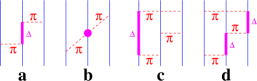
The structure of the two-pion -wave exchange term with an intermediate excitation (Fig. 1a) was originally written down by Fujita and Miyazawa (1957); it can be expressed simply as
| (15) | |||||
where is constructed with the average pion mass and is a sum over the three cyclic exchanges of nucleons . For the Urbana models , as in the original Fujita-Miyazawa model, while other potentials like the Tucson-Melbourne Coon et al. (1979) and Brazil Coelho et al. (1983) models, have a ratio slightly larger than . The shorter-range phenomenological term is given by
| (16) |
For the Urbana IX (UIX) model Pudliner et al. (1995), the two parameters and were determined by fitting the binding energy of 3H and the density of nuclear matter in conjunction with AV18.
While the combined AV18+UIX Hamiltonian reproduces the binding energies of -shell nuclei, it somewhat underbinds light -shell nuclei. A particular problem is that the two-parameter Urbana form is not flexible enough to fit both 8He and 8Be at the same time. A new class of potentials, called the Illinois models, has been developed to address this problem Pieper et al. (2001). These potentials contain the Urbana terms and two additional terms, resulting in a total of four strength parameters that can be adjusted to fit the data. The general form of the Illinois models is
| (17) |
One term, , is due to -wave scattering as illustrated in Fig. 1b and is parametrized with a strength . It has been included in a number of potentials like the Tucson-Melbourne and Brazil models. The Illinois models use the form recommended in the latest Texas model Friar et al. (1999), where chiral symmetry is used to constrain the structure of the interaction. However, in practice, this term is much smaller than the contribution and behaves similarly in light nuclei, so it is difficult to establish its strength independently just from calculations of energy levels.
A more important addition is a simplified form for three-pion rings containing one or two s (Fig. 1c,d). As discussed by Pieper et al. (2001), these diagrams result in a large number of terms, the most important of which are used to construct the Illinois models:
| (18) |
Here the and are operators that are symmetric or antisymmetric under any exchange of the three nucleons, and the subscript or indicates that the operators act on, respectively, spin or isospin degrees of freedom.
The is a projector onto isospin- triples:
| (19) |
To the extent isospin is conserved, there are no such triples in the -shell nuclei, and so this term does not affect them. It is also zero for scattering. However, the term is attractive in all the -shell nuclei studied. The has the same structure as the isospin part of the anticommutator part of , but the term is repulsive in all nuclei studied so far. In -shell nuclei, the magnitude of the term is smaller than that of the term, so the net effect of the is slight repulsion in -shell nuclei and larger attraction in -shell nuclei. The reader is referred to the appendix of Pieper et al. (2001) for the complete structure of .
The first series of five Illinois models (IL1-5) explored different combinations of the parameters , , , and , and also variation of the OPE cutoff function . One drawback of these models is that they appear to provide too much attraction in dense neutron matter calculations Sarsa et al. (2003). To help alleviate this problem, the latest version Illinois-7 (IL7) introduced an additional repulsive term with the isospin- projector:
| (20) |
After fixing at the Texas value, and taking from AV18, the four parameters , , , and were searched to obtain a best fit, in conjunction with AV18, for energies of about 20 nuclear ground and low-lying excited states in nuclei Pieper (2008a).
II.3 Nuclear Hamiltonians from chiral effective field theory
Chiral effective field theory (EFT) has witnessed much progress during the two decades since the pioneering papers by Weinberg (1990, 1991, 1992). In EFT, the symmetries of quantum chromodynamics (QCD), in particular its approximate chiral symmetry, are employed to systematically constrain classes of Lagrangians describing, at low energies, the interactions of baryons (in particular, nucleons and -isobars) with pions as well as the interactions of these hadrons with electroweak fields. Each class is characterized by a given power of the pion mass and/or momentum, the latter generically denoted by , and can therefore be thought of as a term in a series expansion in powers of , where GeV specifies the chiral-symmetry breaking scale. Each class also involves a certain number of unknown coefficients, called low-energy constants (LEC’s), which are determined by fits to experimental data. See, for example, the review papers Bedaque and van Kolck (2002) and Epelbaum et al. (2009), and references therein. Thus EFT provides a direct connection between QCD and its symmetries and the strong and electroweak interactions in nuclei. From this perspective, it can be justifiably argued to have put low-energy nuclear physics on a more fundamental basis. Just as importantly, it yields a practical calculational scheme, which can, at least in principle, be improved systematically.
Within the nuclear EFT approach, a variety of studies have been carried out in the strong-interaction sector dealing with the derivation of and potentials Ordonez et al. (1996); Epelbaum et al. (1998); Entem and Machleidt (2003); Machleidt and Entem (2011); Navratil (2007); Epelbaum et al. (2002); van Kolck (1994); Bernard et al. (2011); Girlanda et al. (2011) and accompanying isospin-symmetry-breaking corrections Friar and van Kolck (1999); Epelbaum and Meissner (1999); Friar et al. (2004, 2005). In the electroweak sector additional studies have been made dealing with the derivation of parity-violating potentials induced by hadronic weak interactions Haxton and Holstein (2013); Zhu et al. (2005); Girlanda (2008); Viviani et al. (2014) and the construction of nuclear electroweak currents Park et al. (1993); Pastore et al. (2009, 2011); Piarulli et al. (2013); Kölling et al. (2009, 2011).
Recently chiral nuclear interactions have been developed that are local up to next-to-next-to-leading order (N2LO) Gezerlis et al. (2013). These interactions employ a different regularization scheme from previous chiral interactions, with a cutoff in the relative momentum . They are therefore fairly simple to treat with standard QMC techniques to calculate properties of nuclei and neutron matter Lynn et al. (2014); Gezerlis et al. (2013).
As explained in Gezerlis et al. (2014), up to N2LO, the momentum-dependent contact interactions can be completely removed by choosing proper local operators. For example, at LO there are several operators that are equivalent for contact interactions: , , , and . Similarly, interactions at NLO and N2LO can be constructed by adding extra operators that include the , , and . The short-range regulators are also chosen to be local, i.e., . In this way, by fitting the low-energy constants, the chiral potentials are completely local up to N2LO. At the next order N3LO non-local operators start to appear, but their contributions are expected to be very small Piarulli et al. (2015).
III Quantum Monte Carlo methods
There is a large variety of Quantum Monte Carlo algorithms, and it would be out of the scope of this review to cover all of them. We will limit ourselves to describing a specific subset of QMC algorithms that has been consistently applied to the many nucleon problem, namely algorithms that are based on a coordinate representation of the Hamiltonian, and that are based on recursive sampling of a probability density or of a propagator. This set of methods includes the standard Variational Monte Carlo (VMC), Green’s Function Monte Carlo (GFMC) and Diffusion Monte Carlo methods.
These methods have been successfully applied to a broad class of problems. The major fields of application of this set of algorithms are quantum chemistry and materials science B.J. Hammond (1994); Nightingale and Umrigar (1999); Foulkes et al. (2001), where QMC is a natural competitor of methods such as Coupled Cluster theory and standard Configuration Interaction methods that are very accurate for problems where the uncorrelated or Hartree-Fock state provides already a good description of the many-body ground state. In these fields several software packages have been developed with the aim of making the use of QMC methods more and more widespread across the community. Other applications in condensed matter theory concern the physics of condensed helium systems, both 4He and 3He Schmidt and Ceperley (1992); Ceperley (1995). Several QMC calculations have been extensively performed to investigate properties of both bosonic and fermionic ultracold gases; see for example Carlson et al. (2003b); Giorgini et al. (2008).
Because of the strong correlations induced by nuclear Hamiltonians, QMC methods have proved to be very valuable in understanding properties of nuclei and nucleonic matter. Variational Monte Carlo methods were introduced for use with nuclear interactions in the early 1980s Lomnitz-Adler et al. (1981). VMC requires an accurate understanding of the structure of the system to be explored. Typically, a specific class of trial wave functions is considered, and using Monte Carlo quadrature to evaluate the multidimensional integrals, the energy with respect to changes in a set of variational parameters is minimized.
GFMC was introduced in nuclear physics for spin- isospin-dependent Hamiltonians in the late 1980s Carlson (1987, 1988). It involves the projection of the ground state from an initial trial state with an evolution in imaginary time in terms of a path integral, using Monte Carlo techniques to sample the paths. GFMC works best when an accurate trial wave function is available, often developed through initial VMC calculations. This method is very accurate for light nuclei, but becomes increasingly more difficult moving toward larger systems. The growth in computing time is exponential in the number of particles because of the number of spin and isospin states. The largest nuclear GFMC calculations to date are for the 12C nucleus Lovato et al. (2013, 2014, 2015), and for systems of 16 neutrons Gandolfi et al. (2011); Maris et al. (2013) (540,672 and 65,536 spin-isospin states, respectively).
Auxiliary Field Diffusion Monte Carlo (AFDMC) was introduced in 1999 Schmidt and Fantoni (1999). In this algorithm the spin- and isospin-dependence is treated using auxiliary fields. These fields are sampled using Monte Carlo techniques, and the coordinate-space diffusion in GFMC is extended to include a diffusion in the spin and isospin states of the individual nucleons as well. This algorithm is much more efficient at treating large systems. It has been very successful in studying homogeneous and inhomogeneous neutron matter, and recently has been shown to be very promising for calculating properties of heavier nuclei, nuclear matter Gandolfi et al. (2014), and systems including hyperons Lonardoni et al. (2013, 2014, 2015). It does require the use of simpler trial wave functions, though, and is not yet quite as flexible in the complexity of nuclear Hamiltonians that can be employed. Extending the range of interactions that can be treated with AFDMC is an active area of research.
III.1 Variational Monte Carlo
In VMC, one assumes a form for the trial wave function and optimizes variational parameters, typically by minimizing the energy and/or the variance of the energy with respect to variations in the parameters. The energy of the variational wave function
| (21) |
is greater than or equal to the ground-state energy with the same quantum numbers as . Monte Carlo methods can be used to calculate and to minimize the energy with respect to changes in the variational parameters.
For nuclear physics, the trial wave function has the generic form:
| (22) |
With this form, a factorization of the wave function into long-range low-momentum components and short-range high-momentum components is assumed. The short-range behavior of the wave functions is controlled by the correlation operator , and the quantum numbers of the system and the long-range behavior by . In nuclei the separation between the short-distance correlations and the low-momentum structure of the wave function is less clear than in some systems. For example, alpha particle clusters can be very important in light nuclei, and their structure is of the order of the interparticle spacing. Also the pairing gap can be a nontrivial fraction of the Fermi energy, and hence the coherence length may be smaller than the system. Nevertheless this general form has proved to be extremely useful in both light nuclei and nuclear matter.
III.1.1 Short-range structure: F
The correlation operator is dominated by Jastrow-like correlations between pairs and triplets of particles:
| (23) |
where is the symmetrization operator, is a two-body and is a three-body correlation. The two-body correlation operator can include a strong dependence upon spin and isospin, and is typically taken as:
| (24) |
where
| (25) |
and the are functions of the distance between particles and . The pair functions are usually obtained as the solution of Schrödinger-like equations in the relative distance between two particles:
| (26) |
The pair functions are obtained by solving this equation in different spin and isospin channels, for example , , and can then be recast into operator form. For =1 channels the tensor force enters and this equation becomes two coupled equations for the components with and .
The are functions designed to encode the variational nature of the calculation, mimicking the effect of other particles on the pair in the many-body system. Additional variational choices can be incorporated into boundary conditions on the . For example, in nuclear and neutron matter the pair functions are typically short-ranged functions and the boundary condition that and at some distances , which may be different in different channels, is enforced. Usually it is advantageous for the tensor correlation to be finite out to longer distances because of the one-pion-exchange interaction. The distances are variational parameters, and the equations for the pair correlations are eigenvalue equations; the eigenvalues are contained in the . See Pandharipande and Wiringa (1979) for complete details.
For the lightest -shell nuclei (A= 3 and 4), on the other hand, the asymptotic properties of the wave function are encoded in the pair correlation operators . To this end the are determined by requiring the product of pair correlations to have the correct asymptotic behavior as particle is separated from the system. These boundary conditions are described in Schiavilla et al. (1986) and Wiringa (1991).
It has been found advantageous to reduce the strength of the spin- and isospin-dependent pair correlation functions when other particles are nearby, with the simple form above altered to
| (27) |
where the central (spin-isospin independent) quenching factor is typically 1, while for other operators it is parametrized so as to reduce the pair correlation when another particle is near the pair Pudliner et al. (1997).
The becomes particularly important when the Hamiltonian includes a force. A good correlation form is:
| (28) |
with , a scaling parameter, and a (small negative) strength parameter. The superscript denotes various pieces of the force like and , so Eq. (28) brings in all the spin-isospin dependence induced by that piece of the potential. In practice the in Eq. (23) is usually replaced with a sum which is significantly faster and results in almost as good a variational energy. For three- and four-body nuclei and nuclear matter, pair spin-orbit correlations have also been included in Eq. (23), but they are expensive to compute and not used in the work reviewed here.
The typical number of variational parameters for s-shell nuclear wave functions is about two dozen for a two-body potential like AV18, as shown in Wiringa (1991) and Pudliner et al. (1997). Another four to six parameters are added if a three-body potential is included in the Hamiltonian. One can also add a few additional parameters to break charge independence, e.g., to generate components in the trinucleon wave functions, but these are generally used only for studies of isospin violation. For -shell nuclei, the alpha-particle pair and triplet correlations are varied only minimally, and most optimization is done with the long-range correlations discussed below.
The variational parameters have generally been optimized by hand. Variational wave functions with significantly larger numbers of parameters and more sophisticated optimization have since been developed Usmani et al. (2009, 2012), but are not in general use. However, they have provided useful insight for improving the simpler parameter sets. The calculation of light nuclei is now sufficiently fast that automated optimization programs might be profitably employed in the future.
III.1.2 Long-Range Structure:
The quantum numbers and long-range structure of the wave function are generally controlled by the term in Eq. (22). For nuclear and neutron matter this has often been taken to be an uncorrelated Fermi gas wave function. Recently, the crucial role of superfluidity has been recognized, particularly in low-density neutron matter. In such cases the trial wave function includes a of BCS form. For the -wave pairing relevant to low-density neutron matter, this can be written:
| (29) |
where the finite particle number projection of the BCS state has been taken, with the individual pair functions, and the unprimed and primed indices refer to spin-up and spin-down particles respectively. These pair states are functions of the distance between the two nucleons in the pair. The operator is an anti-symmetrization operator Carlson et al. (2003a); Gezerlis and Carlson (2008). For a more general pairing, a Pfaffian wave function is needed (see for example Gandolfi et al. (2008a, 2009a) and references therein).
For light nuclei, the simplest can be written as the sum of a few Slater determinants, essentially those arising from a very modest shell-model treatment of the nucleus. The single-particle orbitals in such calculations are written in relative coordinates so as to avoid introducing any spurious center-of-mass (CM) motion. An explicit antisymmetrization of the wave function summing over particles in -wave, -wave, etc., orbitals is required to compute .
Improved wave functions can be obtained by considering the significant cluster structures present in light nuclei. For example the ground state of 8Be has a very large overlap with two well-separated alpha particles. Alpha-cluster structures are important in many light nuclei, for example states in helium and carbon. To this end, it is useful to use a “Jastrow” wave function which includes spin-isospin independent two- and three-body correlations and the cluster-structure for the :
| (30) |
This wave function must be explicitly antisymmetrized as it is written in a particular cluster structure, with particles being in an alpha-particle cluster, summed over the possible partitions. The spin-isospin independent two-body correlations , , and are different for pairs of particles where both are in the -shell, both in the -shell, or one in each. The comes from the structure of an alpha particle, the is constructed to go to unity at large distances. The is set to give the appropriate cluster structure outside the -particle core, for example it is similar to a deuteron for 6Li and to a triton for 7Li; see Pudliner et al. (1997) for more details.
Except for closed-shell nuclei, the complete trial wave function is constructed by taking a linear set of states of the form in Eq. (30) with the same total angular momentum and parity. Typically these correspond to the lowest shell-model states of the system. QMC methods are then used to compute the Hamiltonian and normalization matrix elements in this basis. These coefficients are often similar in magnitude to those produced by a very small shell-model calculation of the same nucleus. In light nuclei coupling is most efficient; examples of the diagonalization may be found in Pudliner et al. (1997); Wiringa et al. (2000); Pieper et al. (2002) and compared to traditional shell model studies such as Kumar (1974). The VMC calculations give very good descriptions of inclusive observables including momentum distributions, but the energies and other observables can then be improved, using the results of the VMC diagonalization to initiate the GFMC calculations.
III.1.3 Computational Implementation
The spatial integrals in Eq. (21) are evaluated using Metropolis Monte Carlo techniques Metropolis et al. (1953). A weight function is first defined to sample points in 3A-dimensional coordinate space. The simplest choice is , where the brackets indicate a sum over all the spin isospin parts of the wave function. For spin-isospin independent interactions the -particle wave function is a function of the coordinates of the system only, and the weight function is the square of the wave function. The Metropolis method allows one to sample points in large-dimensional spaces with probability proportional to any positive function W through a suitable combination of proposed (usually local) moves and an acceptance or rejection of the proposed move based upon the ratio of the function W at the original or proposed points. Iterating these steps produces a set of points in 3A dimensional space with probability proportional to W(R).
For spin-isospin dependent interactions, the wave function is a sum of complex amplitudes for each spin-isospin state of the system:
| (31) |
and the spin states are:
| (32) |
and similarly for the isospin states with and instead of and . The isospin states can be reduced by using charge conservation to states and, by assuming the nucleus has good isospin , further reduced to
| (33) |
components. The weight function in this case is the sum of the squares of the individual amplitudes: .
Given a set of coordinates , to calculate the wave function one must first populate the various amplitudes in the trial state by calculating the Slater determinant, BCS state, or Jastrow wave function . Spin-isospin independent operators acting on are simple multiplicative constants for each amplitude . Pair correlation operators then operate on the ; these are sparse matrix multiplications for each pair. The sparse matrices are easily computed on-the-fly using explicitly coded subroutines Pieper (2008b). The product over pair correlations is built up by successive operations for each pair. For example, the effect of the operator on the wave function of three-particles can be written as follows (The notation means the amplitude for nucleon 1 being spin up and nucleons 2 and 3 being spin down; the isospin components have been omitted for simplicity):
| (50) |
Metropolis Monte Carlo is used to sample points in the 3-dimensional space by accepting and rejecting trial moves of the particles. Enforcing detailed balance ensures that the asymptotic distribution of such points will be distributed according to the weight . The energy can then be computed as the average over the points in the random walk:
| (51) |
where the angled brackets imply the sum over spin and isospin states for each set of spatial coordinates . The matrix elements of the Hamiltonian are evaluated using the same techniques as those used for the pair correlation operators.
The computational time for the VMC method scales exponentially with the particle number. At first glance, this may seem to be because of the explicit sums over exponentially large number of spin-isospin amplitudes calculated from the trial wave function. If that were the only reason, it would be trivial to sample the spin-isospin state and evaluate the trial wave function’s amplitude for that sampled spin-isospin state. This sampling can in fact be done but the fundamental problem remains that good trial wave functions constructed as described in Eqs. (22–24), require exponential in the particle number operations to evaluate either a single spin-isospin amplitude or all of them. Evaluating a single amplitude provides negligible savings, so the computational time is reduced by explicitly summing over the amplitudes, which removes any variance that would occur from sampling. If trial wave functions could be constructed which capture the important physics, while requiring computational time that scales polynomially with particle number for a single spin-isospin amplitude, VMC calculations would be straightforward for all nuclei.
In reality one does not usually compute the full wave function with all orders of pair operators implied by the symmetrization operator in the definition of the wave function. One can sample the orders of the pairs independently for the left and right (bra and ket) wave functions of Eq. (51), and define a slightly more complicated positive definite form for the weight function in terms of the two sets of amplitudes and for the order of pair operators and in the left- and right-hand wave functions. From several thousand to several tens of thousands of points are sufficient for a typical evaluation of the energy, and statistical errors are obtained using standard techniques.
To search for optimal variational parameters embedded in , it is very useful to first generate a Monte Carlo walk with configurations and weights for a given parameter set. Then one can change one or more parameters and reuse the same set of configurations to evaluate the change in the energy. The correlated energy difference will have a much smaller statistical error than differencing two large energies obtained from independent random walks. In this manner, a chain of small incremental improvements can be developed that leads to a lower variational energy. When the norm of the improved wave function starts to differ significantly from the original walk, a new reference walk can be made and the search continued from that set.
One way to overcome the exponential growth in computational requirements and access larger nuclei is to use a cluster expansion. Cluster expansions in terms of the operator correlations in the variational wave function were developed more than two decades ago and used in the first QMC calculations of 16O Pieper et al. (1992). In these calculations a full -dimensional integral was done for the Jastrow part of the wave function while up to four-nucleon linked-clusters were used for the operator terms. Earlier versions of the Argonne and Urbana interactions were used. Given the tremendous increase in computer power since then, this method might profitably be reconsidered for calculations of much bigger nuclei.
III.2 Green’s function Monte Carlo
GFMC methods are used to project out the ground state with a particular set of quantum numbers. GFMC methods were invented in the 1960s Kalos (1962) and have been applied to many different problems in condensed matter, chemistry, and related fields. They are closely related to finite-temperature algorithms which calculate the density matrix Ceperley (1995), but they use trial wave functions on the boundaries of the paths to project out the quantum numbers of specific states.
GFMC typically starts from a trial wave function and projects:
| (52) |
where is a parameter used to control the normalization. For strongly-interacting systems one cannot compute directly, however one can compute the high-temperature or short-time propagator, and insert complete sets of states between each short-time propagator,
| (53) |
and then use Monte Carlo techniques to sample the paths in the propagation. The method is accurate for small values of the time step , and the accuracy can be determined by simulations using several different values of the time step and extrapolating to zero. In the GFMC method, Monte Carlo is used to sample the coordinates ; Eq. (53) also has an implied sum over spin and isospin states at each step of the walk which is calculated explicitly.
III.2.1 Imaginary-Time Propagator
In the simplest approximation the propagator:
| (54) | ||||
where is the non-relativistic kinetic energy:
| (55) |
with , yielding a Gaussian diffusion for the paths. The matrix is the spin- and isospin-dependent interaction:
| (56) |
where indicates a symmetrization over orders of pairs. Each pair interaction can be simply evaluated as the exponent of a small spin-isospin matrix. This treatment is adequate for static spin-dependent interactions.
In practice one needs to include momentum-dependent spin-orbit interactions as well as interactions. It is more efficient to calculate the propagator explicitly, storing the radial and spin-isospin dependence on a grid for each initial and final state. This is done by calculating the propagator independently in each partial wave and then summing them to create the full propagator. This was first done in studies of liquid Helium Ceperley (1995); Schmidt and Lee (1995) and then adapted to the nuclear physics case Pudliner et al. (1997). This has the advantage of summing all interactions for each pair explicitly, allowing for larger time steps in the path-integral simulation. The propagator is defined:
| (57) |
where and are the initial and final relative coordinates, is the Hamiltonian including relative kinetic energy and the interaction, and and are initial and final spin and isospin states, respectively. The pair propagator is calculated for the AV8′ Hamiltonian, denoted as . At present higher order terms in the momenta are treated perturbatively. Though the pair propagator can be calculated for these interactions, the Monte Carlo sampling can lead to large variance Lynn and Schmidt (2012).
The pair propagators are then combined to produce the full propagation matrix for the system. The interaction is included symmetrically, and the full propagation matrix for each step can then be written as:
| (58) |
The spin-orbit interaction in the product of propagators with the full v8 interaction yields spurious interactions resulting from quadratic terms in the difference from different pairs. One can correct for this but in practice the effect is not significant. Using the calculated propagators allows for a factor of 5-10 larger time steps than the simple approximation in Eq.(III.2.1) Pudliner et al. (1997).
III.2.2 Implementation
Once the propagator for each step is specified, an algorithm must be chosen to sample over all possible paths. A branching random walk algorithm very similar to that used in standard diffusion Monte Carlo (DMC) Foulkes et al. (2001) is used. This random walk does not sample the entire path at once; it uses Markov Chain Monte Carlo to perform each step given the present coordinates and amplitudes in the propagated wave function. One difference with standard DMC is that the importance sampled Green’s function is explicitly sampled rather than using a small time-step extrapolation for the wave functions.
A positive definite “weight” is first defined as a function of the trial function and the propagated wave function . Typically the form used is
| (59) |
where is a small parameter. Sampling of the paths and branching for the importance function are then implemented with the scalar function . Given the present position , several different possible final states are sampled from the free propagator . For each sample of the corresponding configuration is included in the sample. The weight function is then calculated for each of the possible new points , and the final point is chosen according to the relative weights and scaled with the ratio of the average to the actual . Branching is performed with the ratio of weight functions after and before the step, or typically after several steps. The weights of different paths used to calculate observables will eventually diverge, yielding the entire contribution from only a few paths that dominate. This is commonly avoided by using the branching technique, in which the configurations are redistributed by killing or making copies of each one according to
| (60) |
where is the weight of the i-th configuration obtained by multiplying the weight of Eq. (59) by ( is the spin/isospin independent part of the potential), is a random number with uniform distribution between 0 and 1, and in the above equation means the truncated integer number of the argument. Different random number seeds are given to new copies generated from the same walker. This procedure guarantees that the configurations with small weight, contributing by generating only noise to the observables, are dropped. The full procedure is described in Pudliner et al. (1997).
After every typically 20 to 40 steps, the energy as a function of imaginary time is calculated as:
| (61) |
where the sum over indicates the sum over samples of the wave function. The brackets in the numerator and denominator of the last expression indicate sums over spins and isospins for each sample. The initially decrease rapidly from the VMC () energy but then stabilizes and just fluctuates within the statistical errors; examples of this are shown in Fig. 2, discussed below, and also in Sec. V.4. These stable values are averaged to get the converged GFMC results.
In principle, the GFMC propagation should converge to the lowest-energy state of given quantum numbers . The nuclei considered here may have a few particle-stable and multiple particle-unstable excited states of the same quantum numbers. In practice, GFMC propagation can obtain good energy estimates for many of these additional states.
First, a set of orthogonal VMC trial functions are generated that are diagonalized in the small single-particle -shell basis of differing and spatial symmetry combinations that can make a given . These are pseudo-bound wave functions that fall off exponentially at long range, with matter radii not much larger than the ground state. Then independent GFMC propagations are carried out starting from each of these trial functions. An example is shown in Fig. 2 for the four -shell states in 7Li, all of which are particle-unstable Pieper et al. (2004). The GFMC propagations stay nearly orthogonal to fairly large MeV-1, as shown by the solid symbols in the figure. The overlaps between different states can be evaluated, and an explicit reorthogonalization made, shown by the open symbols. The states remain well-separated in energy.

The first state in Fig. 2 is physically wide ( keV) because it has the spatial symmetry of alpha plus triton and is several MeV above the threshold for breakup into separated clusters. Consequently, a GFMC propagation is expected to eventually drop to that threshold energy, and the figure shows, after a rapid initial drop from 26 to 32 MeV by MeV-1, a slowly decreasing energy as increases, reaching 33 MeV at MeV-1. In cases like this, the energy is quoted at the small value of where the rapid initial improvement over the variational starting point has saturated. The second state in Fig. 2 is physically narrow ( keV) because it has a spatial symmetry like 6Li+ and is only 20 keV above that breakup threshold. The GFMC propagation shows the same rapid initial drop in energy, and then no appreciable further decline, allowing us to identify a clear energy for this state. The third and fourth states are not experimentally identified, but from the GFMC propagation behavior we would expect the third state to be physically narrow, and the fourth to be fairly broad. An alternative approach to calculate systems in the continuum by imposing specific boundary conditions is presented in sec. IV.6.
In general the GFMC method suffers from the fermion sign problem, in that the numerator and denominator of Eq. (61) tend to have an increasing ratio of error to signal for a finite sample size and large imaginary times . Other than for a few special cases such as purely attractive interactions, Hubbard models at half-filling, or lattice QCD at zero chemical potential, QMC methods typically all have this difficulty. This is basically because when is not exact it contains contamination from the Bosonic ground-state that will be unavoidably sampled. For scalar potentials, or in any case where a real wave function can be used, the sign problem is avoided by using the fixed-node approximation, and the problem is solved in a restricted (Bosonic) sub-space, where the trial wave function always maintains the same sign. In this case the problem would be exactly solved if the nodes of the true ground-state were known. Because this is not the case, the solution obtained is a rigorous upperbound to the true ground-state energy Moskowitz et al. (1982). For spin-isospin dependent Hamiltonians a complex wave function must be used, and the general fixed-node approximation does not apply. Instead the sign problem is circumvented by using a ‘constrained path’ algorithm, essentially limiting the original propagation to regions where the propagated and trial wave functions have a positive overlap. This approximation, like the fixed-node algorithm for spin-independent interaction, involves discarding configurations that have zero overlap with the trial wave function. As such, they are exact for the case when the trial wave function is exact and are therefore variational. However, unlike the fixed-node case, the constrained path method does not provide upper bounds Wiringa et al. (2000).
To address the possible bias introduced by the constraint, all the configurations (including those that would be discarded) for a previous number of steps are used when evaluating energies and other expectation values. is chosen to be as large a number of time steps as feasible with reasonable statistical error (again typically 20 to 40 steps). Tests using different trial functions and very long runs indicate that energies in -shell nuclei are accurate to around one per cent using these methods. This has been tested in detail in Wiringa et al. (2000), where the use of different wave functions is discussed.
Expectation values other than the energy are typically calculated from “mixed” estimates; for diagonal matrix elements this is:
| (62) |
The above equation can be verified by assuming that the true ground state is well represented by the variational wave function and a small perturbation, i.e., , and is a small parameter. Since the variational wave functions are typically very good the extrapolation is quite small. This can be further tested by using different trial wave functions to extract the same observable, or using the Hellman-Feynman theorem. For the case of simple static operators, improved methods are available that propagate both before and after the insertion of the operator Liu et al. (1974), i.e. directly calculating operators with on both sides. However these techniques might be very difficult to apply for non-local operators.
Because a Hamiltonian commutes with itself, the total energy of the Hamiltonian used to construct the propagator [Eq. (58)] is not extrapolated; thus this total energy is not the sum of its extrapolated pieces, rather the sum differs by the amount the energy was improved. As was noted above, the full AV18 potential cannot be used in the propagator; rather an containing the AV8′ approximation to AV18 is used. In practice AV8′ gives slightly more binding than AV18 so the the repulsive part of the potential is increased to make . The difference must be extrapolated by Eq. (62). The best check of the systematic error introduced by this procedure is given by comparing GFMC calculations of 3H and 4He energies with results of more accurate few-nucleon methods; this suggests that the error is less than 0.5% Pudliner et al. (1997).
In the case of off-diagonal matrix elements, e.g., in transition matrix elements between initial and final wave functions, Eq. (62) generalizes to:
| (63) | |||||
Technical details can be found in Pervin et al. (2007).
Recently, the capability to make correlated GFMC propagations has been added Lovato et al. (2015). In these calculations, the values of for every time step, the corresponding weights , and other quantities are saved during an initial propagation. Subsequent propagations for different initial or different nuclei (such as isobaric analogs) then follow the original propagation and correlated differences of expectation values can be computed with much smaller statistical errors than for the individual values.
III.3 Auxiliary Field Diffusion Monte Carlo
The GFMC method works very well for calculating the low lying states of nuclei up to 12C. Its major limitation is that the computational costs scale exponentially with the number of particles, because of the full summations of the spin-isospin states. An alternative approach is to use a basis given by the outer product of nucleon position states, and the outer product of single nucleon spin-isospin spinor states. An element of this overcomplete basis is given by specifying the Cartesian coordinates for the nucleons, and specifying four complex amplitudes for each nucleon to be in a spin-isospin state. A basis state is then defined
| (64) |
The trial functions must be antisymmetric under interchange. The only such functions with polynomial scaling are Slater determinants or Pfaffians (BCS pairing functions), for example,
| (65) |
or linear combinations of them. Operating on these with the product of correlation operators, Eq. (23), again gives a state with exponential scaling with nucleon number. In most of the AFDMC calculations, these wave functions include a state-independent, or central, Jastrow correlation:
| (66) |
Calculations of the Slater determinants or Pfaffians scale like when using standard dense matrix methods, while the central Jastrow requires operations if its range is the same order as the system size. These trial functions capture only the physics of the gross shell structure of the nuclear problem and the state-independent part of the two-body interaction. Devising trial functions that are both computationally efficient to calculate and that capture the state-dependent two- and three-body correlations that are important would greatly improve both the statistical and systematic errors of QMC methods for nuclear problems.
The trial wave functions above can be used for variational calculations. However, the results are poor since the functions miss the physics of the important tensor interactions. More recently the improved form
| (67) |
has been employed, where are spin-isospin independent correlations, and the correlations have a form similar to those discussed in the previous sections. These wave functions can be used as importance functions for AFDMC calculations where they have been found adequate for this purpose in a variety of problems.
Using the basis state as in Eq. (64) requires the use of a different propagator, with at most linear spin-isospin operators. The propagator can be rewritten using the Hubbard-Stratonovich transformation:
| (68) |
where the variables are called auxiliary fields, and can be any type of operator included in the propagator.
It is helpful to apply the auxiliary field formalism to derive the well known central potential diffusion Monte Carlo algorithm Anderson (1976). The Hamiltonian is
| (69) |
and is a generic potential whose form depends on the system. Making the short-time approximation, the propagator can be written as
| (70) |
Since the Hamiltonian does not operate on the spin, the spin variables can be dropped from the walker expressions to leave just a position basis . Operating with the local-potential term gives just a weight factor:
| (71) |
The kinetic energy part of the propagator can be applied by using the Hubbard-Stratonovich transformation:
| (72) | ||||
This propagator applied to a walker generates a new position , where each particle position is shifted as
| (73) |
This is identical to the standard diffusion Monte Carlo algorithm without importance sampling. Each particle is moved with a Gaussian distribution of variance , and a weight of is included. The branching on the weight is then included to complete the algorithm.
The potential in the general form of Eq. (4) can be written as
| (74) |
where are , or similar combinations; see Gandolfi (2007) for more details. The new operators are defined
| (75) |
Here and are the eigenvectors and eigenvalues obtained by diagonalizing the matrix .
It is easy to see that applying the Hubbard-Stratonovich transformation consists in a rotation of the spin-isospin states of nucleons:
| (76) | ||||
The propagation is performed by sampling the auxiliary fields from the probability distribution , and applying the rotations to the nucleon spinors. At order the above propagator is the same as that described in the previous sections. The advantage of this procedure is that a wave function with the general spin-isospin structure of Eq. (65) can be used, at a much cheaper computational cost than that of including all the spin-isospin states of Eq. (31). However, one must then solve the integral in Eq. (68), which is done by Monte Carlo sampling of the auxiliary fields .
The inclusion of importance sampling within the auxiliary fields formalism is straightforward, and is currently done as described in Sec. III.2.2. At each time-step a random vector for the spatial coordinates, and the required auxiliary fields are sampled. The four weights corresponding to these samples are
| (77) |
where is used for the importance sampling, are obtained by rotating the spinors of the previous time-step using the auxiliary fields , and includes all the spin-isospin independent terms of the interaction. The procedure is then completed as done in GFMC: one of the above configurations is taken according to the probabilities, and the branching is done by considering the cumulative weight. This procedure lowers the variance as the ”plus-minus” sampling cancels the linear terms coming from the exponential of Eqs. (72,76). Note that in the example of the kinetic energy presented above, the effect of sampling using is identical to sampling configurations using commonly adopted in standard diffusion Monte Carlo Foulkes et al. (2001).
The importance function must be real and positive, and an efficient algorithm to deal with complex wave functions has been proposed by Zhang and Krakauer (2003), i.e., consider , and multiply the weight terms by , where is the phase of , and for each , is the corresponding configuration obtained from the corresponding and sampling. This method samples configurations with a very low variance.
Previous applications of the AFDMC method used a somewhat different importance sampling, using for the kinetic energy, and the strategy described by Sarsa et al. (2003) and Gandolfi et al. (2009b) for the spin; the two methods become the same in the limit of . In Gandolfi et al. (2014) it has been found that the procedure described above is much less time-step dependent for calculations including protons. This is due to the strong tensor force in the channel that in the case of pure neutron systems is very weak. The two algorithms give very similar results.
The energy and other observables are calculated after a block of steps in imaginary time, where each block comprises a number of steps that is chosen to be large enough (typically around 100-500) such that the configurations are statistically uncorrelated. This is done to save computing time in calculating observables for data that are not useful to reduce the statistical errors.
While the Hubbard-Stratonovich transformation is the most common, there are many other possibilities. For example, the propagator for the relativistic kinetic energy can be sampled by using
| (78) |
with
| (79) |
where is the modified Bessel function of order 2 Carlson et al. (1993).
IV Light nuclei
IV.1 Energy spectra
Results of GFMC calculations for light nuclei using the AV18+IL7 Hamiltonian are compared to experiment in Fig. 3 and Table 1 Brida et al. (2011); McCutchan et al. (2012); Pastore et al. (2013); Lovato et al. (2013); Wiringa et al. (2013); Pastore et al. (2014); Pieper and Carlson (2015). Results using just AV18 with no potential are also shown in the figure. Figure 3 shows the absolute energies of more than 50 ground and excited states. The experimental energies of the 21 ground states shown in the table are reproduced with an rms error of 0.36 MeV and an average signed error of only 0.06 MeV. The importance of the three-body interaction is confirmed by the large corresponding numbers for AV18 with no potential, namely 10.0 and 8.8 MeV. About sixty additional isobaric analog states also have been evaluated but are not shown here.
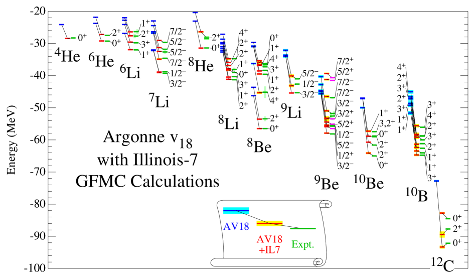
Table 1 gives the ground state energies , proton (neutron) point radii (), magnetic moments (including two-body current contributions, see Sec. V), and quadrupole moments for all the particle-stable ground states of nuclei, plus 12C and the resonant ground states of 7He and 8Be. Many of these results were obtained in recent studies of spectroscopic overlaps, electromagnetic transitions and sum rules, and isospin mixing. The energies, radii, and electromagnetic moments are in generally good agreement with experiment.
| (MeV) | [] (fm) | () | (fm2) | ||||||
|---|---|---|---|---|---|---|---|---|---|
| GFMC | Expt. | GFMC | Expt. | GFMC | Expt. | GFMC | Expt. | ||
| 2H | |||||||||
| 3H | |||||||||
| 3He | |||||||||
| 4He | |||||||||
| 6He | |||||||||
| 6Li | |||||||||
| 7He | |||||||||
| 7Li | |||||||||
| 7Be | |||||||||
| 8He | |||||||||
| 8Li | |||||||||
| 8Be | |||||||||
| 8B | |||||||||
| 8C | |||||||||
| 9Li | |||||||||
| 9Be | |||||||||
| 9C | |||||||||
| 10Be | |||||||||
| 10B | |||||||||
| 10C | |||||||||
| 12C | |||||||||
A detailed breakdown of the AV18+IL7 energies into various pieces for some of the nuclear ground states is shown in Table 2. The components include the total kinetic energy , the contribution of the strong interaction part of AV18, the full electromagnetic potential , the two-pion-exchange parts of IL7 , the three-pion-ring parts , and the short-range repulsion . In the last column, is the expectation value of the difference between and , which is the part of the interaction that is treated perturbatively because is used in the propagation Hamiltonian. The sum of the six contributions through does not quite match the total energy reported in Table 1 because they have been individually extrapolated from the mixed energy expression Eq. (62).
Several key observations can be drawn from Table 2. First, there is a huge cancellation between kinetic and two-body terms. Second, the net perturbative correction is tiny () compared to the full expectation value. Third, the total contribution is of , suggesting good convergence in many-body forces, but it is not negligible compared to the binding energy. Finally, the contribution that is unique to the Illinois potentials is a small fraction of the in states, but does get as large as 35% in states.
| 2H | |||||||
|---|---|---|---|---|---|---|---|
| 3H | |||||||
| 4He | |||||||
| 6He | |||||||
| 6Li | |||||||
| 7He | |||||||
| 7Li | |||||||
| 8He | |||||||
| 8Li | |||||||
| 8Be | |||||||
| 9Li | |||||||
| 9Be | |||||||
| 10Be | |||||||
| 10B | |||||||
| 12C |
In describing the structure of the light nuclei, it is convenient to characterize specific states by their dominant orbital and spin angular momentum and spatial symmetry where denotes the Young diagram for spatial symmetry Wiringa (2006). (This classification is essentially a modern update of the discussion in Feenberg and Wigner (1937).) For example, 4He is a [4] state, and the ground state of 6Li is predominantly [42], with admixtures of [42] and [411]. Because forces are strongly attractive in relative -waves, and repulsive in -waves, ground states of given have the maximum spatial symmetry allowed by the Pauli exclusion principle. For the same spatial symmetry, states of higher are higher in the spectrum. Further, due to the effect of spin-orbit forces, iterated tensor forces and also forces, the spin doublets, triplets, etc., are split, with the maximum value for given lying lowest in the spectrum (up to mid -shell). These features are evident in the excitation spectra discussed next.
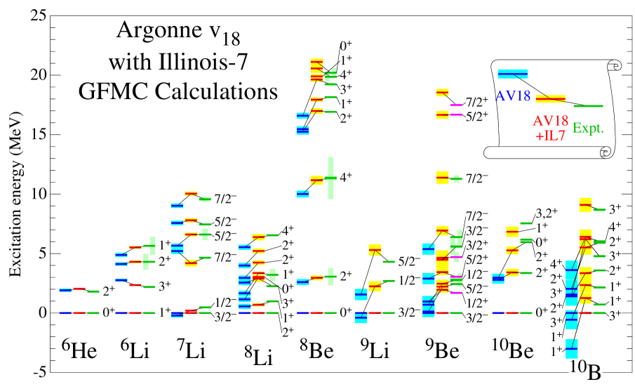
The excitations relative to the ground state energies for many states are shown in Fig. 4 and tabulated in Table 3. These excitation energies are each the difference of two independent GFMC calculations; the quoted statistical errors are the uncorrelated combination of the errors of each calculation. In general, the excitation energies are quite satisfactory with an rms error of 0.5 MeV for 58 states using AV18+IL7 compared to 1.8 MeV using just AV18. Thus we see that AV18 alone does a much better job on excitation energies than it does for absolute binding, and that the addition of IL7 greatly improves both aspects.
The 6He ground state is a [42] combination, with a [42] first excited state; the AV18+IL7 Hamiltonian gets an excitation in fair agreement with experiment. The first three excited states in 6Li constitute a [42] triplet, and the spin-orbit splitting between the , , and states is also reproduced very nicely. The first two states in 7Li are a narrowly split [43] pair, while the next two are a [43] pair, followed by the lowest member of a [421] triplet, all with a reasonably good reproduction of experiment. The 8Be nucleus exhibits a strong rotational spectrum, with a [44] ground state and widely spaced [44] and [44] excited states, also with excitation energies in excellent agreement with experiment. Above this rotational band are [431], [431], and [431] states that isospin mix with the isobaric analogs of the 8Li ground and first two excited states.
The nuclei, which are mid -shell nuclei, have the interesting feature of having two linearly independent ways of constructing [442] states. In 10Be, the ground state is [442] (much like 6He with an added ) followed by two [442] excited states. In 10B, the lowest state might be expected to be a [442] state similar to 6Li ground state plus an , but there are also two [442] triplets, one of which is so widely split by the effective one-body spin-orbit force that one [442] component becomes the ground state leaving the [442] state as the first excited state Kurath (1979).
The IL7 force plays a key role in getting these spin-orbit splittings correctly. The AV18 force alone splits the 6Li [42] states in the correct order, but with insufficient spacing. It leaves the 7Li [43] doublet degenerate, as well as the two [442] states in 10Be, and the [442] state in 10B is predicted to be the ground state. IL7 not only splits the two states in 10Be by about the correct amount, but splits them in the correct direction, making the predicted transitions to the ground state significantly different in size as experimentally observed McCutchan et al. (2012). By increasing the splitting of the [442] states in 10B, IL7 also gives the correct ground state for 10Be. Addition of the older Urbana potentials fixes some, but not all of these problems. The superior behavior of the Illinois interactions is also seen in 5He, i.e., scattering, as discussed in Sect. IV.6. The importance of interactions is also observed in no-core shell model calculations Navrátil et al. (2007).
| GFMC | Expt. | |
|---|---|---|
| 6He | ||
| 6Li | ||
| 6Li | ||
| 6Li | ||
| 7Li | ||
| 7Li | ||
| 7Li | ||
| 7Li | ||
| 8He | ||
| 8Li | ||
| 8Li | ||
| 8Be | ||
| 8Be | ||
| 8Be | ||
| 8Be | ||
| 8Be | ||
| 9Li | ||
| 9Be | ||
| 9Be | ||
| 10Be | ||
| 10Be | ||
| 10B | ||
| 10B | ||
| 10B |
IV.2 Isospin breaking
Energy differences among isobaric analog states are probes of the charge-independence-breaking parts of the Hamiltonian. The energies for a given isospin multiplet can be expanded as
| (80) |
where , , , and are orthogonal isospin polynomials Peshkin (1960). GFMC calculations of the coefficients for a number of isobaric sequences and various contributions for the AV18+IL7 Hamiltonian are shown in Table 4 along with the experimental values. The contributions are the CSB component of the kinetic energy , all electromagnetic interactions , and the strong CIB interactions, . The experimental values were computed using ground-state energies from NNDC (2014) and excitation energies from TUNL (2014). By using the correlated GFMC propagations described in Sec. III.2, it is possible to extract statistically significant values for some of the . An additional contribution is the second-order perturbation correction to the CI part of the Hamiltonian due to differences in the wave functions. Although this term is small, it is the difference between two large energies and has the greatest Monte Carlo statistical error of any of the contributions; again correlated GFMC propagations make its extraction possible.
| Total | Expt. | |||||
|---|---|---|---|---|---|---|
| 14 | 670(1) | 65(0) | 8(1) | 755(1) | 764 | |
| 18 | 1056(1) | 44(0) | 68(3) | 1184(4) | 1174 | |
| 23 | 1478(2) | 83(1) | 27(10) | 1611(10) | 1644 | |
| 17 | 1206(1) | 45 | 85(4) | 1358(3) | 1326 | |
| 25 | 1675(1) | 77 | 43(6) | 1813(6) | 1770 | |
| 22 | 1557(1) | 63 | 104(4) | 1735(3) | 1651 | |
| 19 | 1713(6) | 55(1) | 1786(7) | 1851 | ||
| 26 | 1976(1) | 91(0) | 84(7) | 2176(7) | 2102 | |
| 25 | 2155(7) | 85(1) | 2170(8) | 2329 | ||
| 153(1) | 112(2) | 5(4) | 270(5) | 223 | ||
| 106(0) | 34(1) | 13(2) | 158(5) | 137 | ||
| 136(1) | 3(2) | 10(5) | 139(5) | 127 | ||
| 130(0) | 38(0) | 9(2) | 178(1) | 151 | ||
| 150(1) | 44(1) | 4(5) | 200(4) | 176 | ||
| 178(1) | 119(18) | 297(19) | 241 | |||
| 3(0) | 0(0) | 0(2) | 3(1) | 20(8) | ||
| 1(0) | 0(0) | 1(1) | 2(1) | 3(1) | ||
| 1(1) | 0(0) | 0(4) | 1(3) | 2(5) |
The dominant piece in all these terms is the Coulomb interaction between protons, giving 85-95% (70-100%) of the experimental isovector (isotensor) total. However the strong CSB and CD interactions give important corrections, and the other terms are not negligible. In particular, the contribution is just the right size to fix the 3He – 3H mass difference and is a strong constraint on the difference of and scattering lengths. Overall, the isoscalar terms are in good agreement with experiment, while the isotensor terms are perhaps a little too large. One can understand the negative values of as coming from the increasing Coulomb repulsion as increases; this expands the nucleus and reduces .
Another place that CSB interactions play a role is in the isospin mixing of nearby states with the same spin and parity but different isospins Wiringa et al. (2013). A classic case is the appearance in the 8Be excitation spectrum of three pairs of states with of (at 16.6–16.9 MeV), (at 17.6–18.2 MeV) and (at 19.0–19.2 MeV). The unmixed states come from three states, including the second excitation and first and states in the 8Be spectrum and three states that are the isobaric analogs of 8Li ground state and its first two excited states. These states have the same dominant [431] spatial symmetry, so it is not surprising that their energies are closely paired. The CSB components of the Hamiltonian have keV off-diagonal (in isospin) matrix elements leading to significant isospin mixing.. Experimentally this is observed in the two-alpha decay of the states, which have comparable widths and which can only go via the component of the wave functions. The mixing of the doublet is apparent in their decays Pastore et al. (2014).
GFMC calculations of the isospin-mixing matrix elements are shown in Table 5. The table includes a small contribution from class IV CSB terms that can connect and pairs Henley et al. (1979). The theoretical total provides about 90% of the inferred experimental values in the and doublets, but is too large for the (poorly determined) case.
| Total | Expt. | |||||
|---|---|---|---|---|---|---|
| -4 | -99(1) | -23 | -2(1) | -128(2) | -145(3) | |
| -3 | -74(1) | -19 | 3(1) | -93(2) | -103(14) | |
| -3 | -87(1) | -17 | -6(2) | -113(3) | -59(12) |
IV.3 Densities
The one- and two-nucleon density distributions of light nuclei are interesting in a variety of experimental settings. They are evaluated as the expectation values
| (81) | ||||
| (82) |
where is a proton or neutron projector.
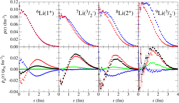
Ground state proton and neutron rms point radii are tabulated in Table 1. These can be related to the charge radii, which have been measured very accurately for the helium, lithium, and beryllium isotopic chains in recent years by a combination of electron scattering from stable nuclei and isotopic differences by atomic spectroscopy on rare isotopes. A recent review Lu et al. (2013) discusses these developments and the conversion between point and charge radii and presents figures for the GFMC one- and two-body densities of the helium isotopes.
The proton and neutron one-body densities for the lithium isotope chain are shown, as red up triangles and blue down triangles, respectively, in the upper panels of Fig. 5. As the binding energy increases with , the central proton density increases, even though the number of protons is constant. Consequently, the proton point radius decreases by 0.4 fm in going from 6Li to 9Li, in fair agreement with the experimentally observed reduction of 0.34 fm. In contrast, the neutron point radius is relatively constant, even though neutrons are being added, varying only 0.15 fm over the same range.
The magnetic moments of nuclei have been calculated in GFMC Pervin et al. (2007); Marcucci et al. (2008); Pastore et al. (2013) including contributions from two-body meson-exchange currents (MEC), as discussed in Sec. V. The MEC can give 20–40% contributions over the impulse approximation (IA) values, resulting in very good agreement with experiment as shown in Table 1.
The origin of the IA contributions from the proton and neutron spin densities and proton orbital density are illustrated in the bottom panels of Fig. 5, also for the lithium isotope chain. Here, the proton spin contribution is shown by red upward-pointing triangles, the neutron spin contribution by blue downward-pointing triangles, the proton orbital contribution by green diamonds, and the total by black circles. The proton spin density, due to one unpaired -shell proton, is similar in all cases, with a negative region at short distance from the core and a positive peak near 2 fm that gradually shifts inward as the binding increases. The neutron spin density has the opposite sign and alternates between a significant unpaired neutron contribution in 6,8Li and a very small paired contribution in 7,9Li. The proton orbital piece gets progressively larger as increases. The MEC contributions are discussed in more detail below, but come largely from pion exchange and are primarily isovector in character, ranging from 2% in 6Li to 10% in 7Li and 20% in 8,9Li.
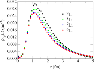
The two-nucleon density for pairs in the lithium isotopes is shown in Fig. 6 and all four curves integrate to three pairs. Because the third proton is in the -shell, the behavior of is rather different from the one pair in the core of the helium isotopes shown in Fig. 12 of Lu et al. (2013). In that case, there is a slight decrease in the peak value as increases because the -shell neutrons in 6,8He tug the core protons out a little. In lithium the peak value of gets progressively larger with increasing due to the increasing binding, so the pair rms radius decreases from 4.03 fm in 6Li to 3.20 fm in 9Li.
IV.4 Momentum distributions
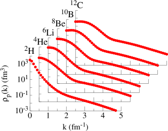
Momentum distributions of individual nucleons, nucleon pairs, and nucleon clusters reflect features of the short-range structure of nuclei. They can provide useful insight into various reactions on nuclei, such as and electrodisintegration processes or neutrino-nucleus interactions.
The probability of finding a nucleon with momentum and spin-isospin projection , in a given nuclear state is proportional to the density
| (83) |
is the spin-isospin projection operator for nucleon , and is the nuclear wave function with total spin and spin projection . The normalization is
| (84) |
where is the number of spin-up or spin-down protons or neutrons.
Early variational calculations of few-nucleon momentum distributions Schiavilla et al. (1986) evaluated Eq. (IV.4) by following a Metropolis Monte Carlo walk in the space and one extra Gaussian integration over at each Monte Carlo configuration. This was subject to large statistical errors originating from the rapidly oscillating nature of the integrand for large values of .
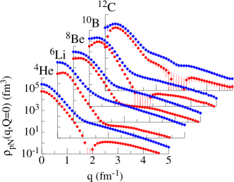
A more efficient method is to rewrite Eq. (IV.4) as
| (85) |
and perform the Gaussian integration over . However, this requires re-evaluating both initial and final wave functions at multiple configurations, which limits the present calculations to VMC. A comprehensive set of single-nucleon momentum distributions for nuclei, evaluated with the AV18+UX Hamiltonian, has been published Wiringa et al. (2014) with figures and tables available on-line Wiringa (2014a).
The overall evolution of the proton momentum distribution in light nuclei is shown in Fig. 7. The shape of the distributions shows a smooth progression as nucleons are added. As increases, the nuclei become more tightly bound, and the fraction of nucleons at zero momentum decreases. As nucleons are added to the -shell, the distribution at low momenta becomes broader, and develops a peak at finite . The sharp change in slope near fm-1 to a broad shoulder is present in all these nuclei and is attributable to the strong tensor correlation induced by the pion-exchange part of the potential, further increased by the two-pion-exchange part of the potential. Above fm-1, the bulk of the momentum density appears to come from short-range spin-isospin correlations.
Two-nucleon momentum distributions, i.e., the probability of finding two nucleons in a nucleus with relative momentum and total center-of-mass momentum , provide insight into the short-range correlations induced by a given Hamiltonian. They can be formulated analogously to Eqs. (IV.4,IV.4), and projected with total pair spin-isospin , or as , , and pairs. Again, a large collection of VMC results has been published Wiringa et al. (2014) and figures and tables are available on-line Wiringa (2014b).
Experiments to search for evidence of short-range correlations have been a recent focus of activity at Jefferson Laboratory. In an experiment on 12C at JLab, a very large ratio of to pairs was observed at momenta =1.5–2.5 fm-1 for back-to-back () pairs Subedi et al. (2008). VMC calculations for are shown in Fig. 8 as blue diamonds for pairs and red circles for pairs for nuclei from 4He to 12C Schiavilla et al. (2007); Wiringa et al. (2014). The back-to-back pairs are primarily in states and have a node near 2 fm-1, while the pairs are in deuteron-like states where the -wave fills in the -wave node. Consequently, there is a large ratio of to pairs in this region. This behavior is predicted to be universal across a wide range of nuclei.
As increases, the -wave node in pairs will gradually fill in, as illustrated for 4He in Fig. 9, where is shown as a function of for several fixed values of , averaged over all directions of and . In contrast, the deuteron-like distribution in pairs is maintained as increases, as shown in Fig. 10, with only a gradual decrease in magnitude because there are fewer pairs at high total . Recently, these momentum distributions for 4He have been tested in new JLab experiments and found to predict the ratio of to pairs at higher missing momentum very well Korover et al. (2014).
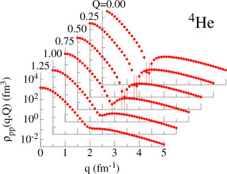
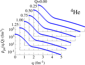
IV.5 Spectroscopic overlaps, spectroscopic factors, and ANCs
Determining the influence of nuclear structure on nuclear reactions is a challenging subject. One source of theoretical input is the calculation of spectroscopic overlaps, spectroscopic factors (SFs), and asymptotic normalization coefficients (ANCs). They are steps on the way to calculating reaction cross sections in direct nuclear reactions, like nucleon knockout or radiative capture.
A one-nucleon spectroscopic overlap is the expectation value of the nucleon removal operator between states of nuclei differing by one particle. It can be written as
| (86) | |||||
where denotes the quantum numbers of a parent -body nucleus, specifies an -body core, and specifies the valence nucleon. Here is the distance between the valence nucleon and the center of mass of the core, and is the valence angle-spin-isospin function. The SF is then defined as the norm of the overlap:
| (87) |
In standard shell model calculations Cohen and Kurath (1967), the SFs obey various sum rules Macfarlane and French (1960), including that for a given state of the parent nucleus, the SFs to all possible final states of the core plus valence nucleon add up to the parent’s number of such nucleons. For example, because 7Li has one -shell proton.
Overlap functions satisfy a one-body Schrödinger equation with appropriate source terms Pinkston and Satchler (1965). Asymptotically, at , these source terms contain core-valence Coulomb interaction at most, and hence the long-range part of overlap functions for parent states below core-valence separation thresholds is proportional to a Whittaker function :
| (88) |
where depends on proton numbers and , the fine-structure constant , and the core-valence reduced mass and the separation energy (negative for parent states below core-valence separation thresholds). The wave number is defined as , and is the orbital momentum in . The proportionality constant in Eq. (88) is the ANC.
VMC calculations of overlaps and SFs for -shell nuclei were first reported in Schiavilla et al. (1986), followed by calculations in various -shell nuclei for application to experiments Lapikás et al. (1999), transfer reactions like and Wuosmaa et al. (2005, 2008), and single-neutron knockout reactions Grinyer et al. (2011, 2012). The first GFMC calculations for nuclei were reported in Brida et al. (2011). These are off-diagonal calculations, as in Eq. (63), so the final GFMC result is extrapolated from two different mixed estimates, one where is propagated for the -body nucleus and one where it is propagated for the -body nucleus. A large collection of VMC and GFMC results can be found on-line Wiringa and Brida (2014).
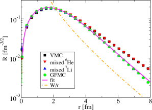
For the -shell nuclei, VMC energies and densities are very close to the exact GFMC results, so VMC and GFMC overlaps for cases like are in excellent agreement, both in the peak values at small and in the asymptotic regime. This translates into very similar SF and ANC predictions. However, for -shell nuclei, the VMC energies are progressively smaller in magnitude relative to GFMC as increases, although the one-body densities remain fairly close. Consequently the overlaps have similar peak values but different asymptotic behavior.
An example of -shell overlap calculations is shown in Fig. 11 for . The VMC calculation is shown by black squares, the two GFMC mixed estimates by red down (blue up) triangles for GFMC propagation of the 6He (7Li) states, and the final GFMC result by green circles. In this case, the VMC overlap and the GFMC mixed estimate when 6He is propagated give virtually identical results, so the GFMC mixed estimate when 7Li is propagated coincides with the final result. The smooth fit to the GFMC result shown by the solid purple line is parallel at large to the Whittaker function (constructed with the experimental separation energy) shown by the dot-dash orange line. The integrated VMC and GFMC SFs for this case are 0.44 and 0.41, respectively. These values are consistent with experiment Lapikás et al. (1999); Wuosmaa et al. (2008) but much smaller than the standard shell model value (corrected for center of mass) of 0.69 Cohen and Kurath (1967).
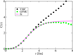
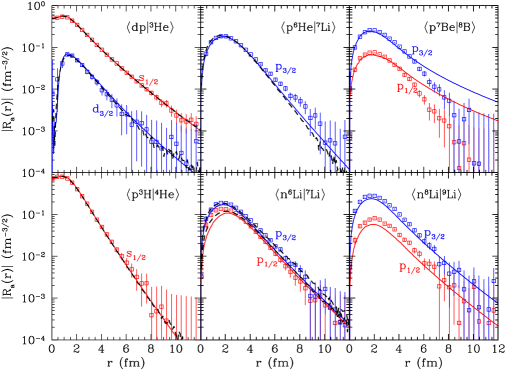
In general, the SFs predicted by the VMC and GFMC calculations show a significant quenching relative to standard shell model estimates which are based on notions of independent particle motion. The low-energy states of light nuclei can be interpreted as having quasiparticles in single-particle orbitals Pandharipande et al. (1997). The difference between physical particles and quasiparticles is the consequence of the correlations in the system, which push a significant fraction of nucleons above the nominal Fermi sea, as noted in the momentum distribution calculations of Sec. IV.4. The SF is the quasihole strength, i.e., the probability of the quasiparticle being a physical particle. A variety of experiments find that, for a broad range of nuclei from 4He to 208Pb, SFs are quenched relative to standard shell model, consistent with the VMC and GFMC calculations Kay et al. (2013).
The ratio of the VMC and GFMC overlaps with the Whittaker function constructed with the experimental separation energy are shown in Fig. 12. The incorrect asymptotic behavior of the VMC calculation means the does not reach a constant value and precludes extracting a reasonable ANC from this ratio. However the GFMC calculation, with its much better asymptotic behavior, does go to a constant at large , as indicated by the purple line fit.
There is an alternative method to obtain overlaps, ANCs, and estimates of widths from variational wave functions using integral constraints that are insensitive to their asymptotic behavior Barletta et al. (2009); Nollett and Wiringa (2011); Nollett (2012). As an example, the ANC is given by a sort of modified overlap integral with a finite-range potential insertion:
The integral extends over all particle coordinates, is an antisymmetrization operator for the core and valence particle, is the Whittaker function that is irregular at infinity, and is its Wronskian with the regular Whittaker function . The is a sum of two- and three-body potentials involving the last nucleon
| (90) |
where we have labeled the last nucleon . The point-Coulomb potential between the residual nucleus and last nucleon is and in the limit of large separation, typically fm, vanishes. This provides a natural cutoff to the integral of Eq. (IV.5).
This integral method has been implemented, using VMC wave functions obtained for the AV18+UIX Hamiltonian, for 19 one-nucleon removals from nuclear states with . Detailed tables are given in Nollett and Wiringa (2011), as well as comparisons to available experimental determinations and previous theoretical work. In general, when the experimental binding energy is used in the wave number , the ANCs derived from VMC wave functions through Eq. (IV.5) are in excellent agreement with experiment. The results also agree with the GFMC determinations discussed above at level, e.g., the GFMC ANC for from Fig. 12 is 3.5, while the VMC integral value is 3.7. Of particular note, the astrophysical -factor for is related to the ANCs by Esbensen (2004). Inserting the VMC ANC values gives the result 20.8 eV b, which is exactly the current recommended value from the Solar Fusion II analysis Adelberger et al. (2011).
Relations similar to Eq. (IV.5) can be used to generate overlaps and also to estimate the widths of resonant states Nollett (2012). Examples of overlaps evaluated in this way are shown in Fig. 13, where they are compared to the VMC input and the GFMC overlaps of Brida et al. (2011). Many widths in nuclei have also been evaluated, using as input VMC pseudo-bound wave functions from the AV18+UIX Hamiltonian. Detailed tables are given in Nollett (2012). The agreement with experiment is generally satisfactory when the physical states are narrow, but the method fails for broad states; the overlaps can help differentiate these cases. For broad states, true scattering wave functions need to be developed, as discussed below.
While the preceding discussion has focused on single-nucleon spectroscopic overlaps, SFs, ANCs, and widths, the techniques involved are readily adaptable to other cluster-cluster pairings, e.g., with deuterons or s as the valence cluster. Spectroscopic overlaps for in 4He, in 6Li, and in 7Li are included in the on-line overlap tabulations of Wiringa and Brida (2014) and spectroscopic factors can be obtained from the cluster-cluster momentum distribution tables in Wiringa (2014a). It should be possible in future to evaluate ANCs and widths from the VMC wave functions and generalized integral relations.
IV.6 Low-Energy Scattering
Quantum Monte Carlo methods can also be used to treat low-energy scattering in nuclear systems Carlson et al. (1987); Nollett et al. (2007). The methods employed are similar to bound-state methods, and are easily applicable at low energies where the combined system breaks up into at most two clusters. One enforces one or more boundary conditions on the asymptotic wave function at large cluster separations and then solves for the energy levels with these boundary conditions. The resulting energies can be used with the boundary conditions to determine the elements of the -matrix for those energies.
The simplest example is for a one-channel case with only elastic scattering, for example scattering. The asymptotic wave function for the relative motion of the neutron and the alpha particle is given by:
| (91) |
where and are the internal wave functions of the two clusters, and are the relative momentum and spatial separation between the two clusters, and is the phase shift in the partial wave. For problems with Coulomb interactions between the clusters the relative wave function will contain Coulomb rather than Bessel functions.
The original QMC scattering calculations required the wave function to be zero at a specified cluster separation Carlson et al. (1987), while in recent work the logarithmic derivative of the relative wave function at a boundary is specified Nollett et al. (2007):
| (92) |
In VMC calculations this is enforced within the form of the trial wave function, which is required at large distances to go like Eq. (91). The radius should be large enough so that there is no strong interaction between the clusters at that separation. The scattering energy and hence the relative momentum between clusters is unknown initially, but these are obtained by variationally solving for states confined within the boundary . Knowledge of the energy and the boundary condition is then sufficient to determine the phase shift at that energy. The method for GFMC is very similar, except that the logarithmic derivative of the wave function must also be enforced in the propagator. This can be incorporated through an image method. For each point near the boundary reached during the random walk, the contribution to the internal wave function from points originally outside the boundary are added. Consider an image at a cluster separation ; simple manipulations yields
| (93) | ||||
where and are the initial and final points of all the particles, and are the internal coordinates of the clusters, and is the separation between clusters. The image point for all the particles is denoted by , and is its cluster separation. The image contribution ensures the correct logarithmic derivative of the wave function at the boundary is preserved in the propagation.
The system is interesting as it is the lightest system where triplets play a significant role. QMC methods have been used to study low-energy scattering in , including the two low-lying -wave resonances and -wave scattering Nollett et al. (2007). The spin-orbit splitting is especially interesting, as it can be examined by comparing the and partial waves.
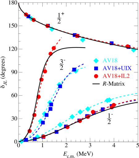
The results of calculations with the AV18 interaction and with different interactions are shown in Fig. 14. The various calculations are also compared with an -matrix analysis of the experimental data. As is evident from the figure, the AV18 interaction alone significantly underpredicts the spin-orbit splitting. The two-pion-exchange in the UIX interaction increases the splitting, but not enough to agree with the experimental data. The IL2 model of the interaction results in good agreement with the experimental spin-orbit splitting.
These scattering methods have many possible applications. They can be extended to inelastic multichannel processes in a fairly straightforward manner. In this case there are multiple independent solutions for a given scattering energy, hence one must study the energy as a function of the boundary conditions in each channel and obtain multiple independent solutions for the same energy. From the boundary conditions, the energy, and the relative asymptotic magnitude of the wave functions, one can obtain the full multichannel -matrix. It should be possible to treat a variety of low-energy strong reactions, as well as electroweak transitions involving scattering states using these methods. In addition, hadronic parity violation in few-nucleon systems is an important application.
IV.7 Chiral Interactions
Local potentials derived within chiral effective field theory have been used to calculate properties of A=3,4 nuclei with GFMC by Lynn et al. (2014). Although the calculations do not yet include interactions that also appear at N2LO, they are nevertheless interesting, showing the order-by-order results for the binding energies and also the range of results for different cutoffs. Also the question of perturbative treatments of higher-order corrections has been investigated, as well as one- and two-nucleon distributions.
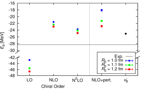
Figure 15 shows results at various orders and for different values of the cutoff used to regulate the small- behavior of the pion-exchange potentials, . The LO result is extremely overbound, whereas the NLO and N2LO results are underbound as expected because of the lack of the interaction. The NLO interaction includes pion-exchange diagrams, and the N2LO two-pion exchange terms. On the right, the column labeled ‘NLO+pert’ shows the results for the N2LO binding energy using the NLO wave function plus the perturbative contribution of the difference between the two interactions. The perturbative treatment is reasonable, but the spread of energies is significantly larger and of course the binding is less than in the full nonperturbative calculation. The role of chiral interactions in light nuclei and in matter are currently being investigated.
It should be noted that lattice QMC approaches to the study of chiral interactions have been pursued Lee et al. (2004); Epelbaum et al. (2011, 2012, 2014). These methods have also been used to study, for example, the Hoyle state in 12C and the ground state and excitations in 16O. While the lattices used to date are rather coarse, using a lattice spacing near 2 fm corresponding to a maximum momenta of 1.5 fm-1, they obtain very good results for the energies of the Hoyle state and for other nuclei with alpha particle substructure. Comparisons for different forms of chiral interactions and for a variety of observables could prove very valuable.
V Electroweak currents
V.1 Conventional nuclear electroweak currents
A fundamental aspect in the description of electroweak processes in nuclei is the construction of a realistic set of nuclear electroweak currents. The electromagnetic current is denoted by , and the neutral and charge-changing weak currents as and , respectively. In the Standard Model of particle physics, the latter consist of polar-vector ( or ) and axial-vector () parts, and read
| (94) |
where is the Weinberg angle ( Nakamura (2010)), and are, respectively, the isoscalar and isovector pieces of the electromagnetic current, and the subscript with =, , or on , , and denotes components in isospin space. The conserved-vector-current constraint relates the polar-vector components of the charge-changing weak current to the isovector component of the electromagnetic current via
| (95) |
where are isospin operators, the implication being that form a vector in isospin space. There are in principle isoscalar contributions to associated with strange quarks, but they are ignored in Eq.(V.1), since experiments at Bates Spayde et al. (2000); Beise et al. (2005) and Jefferson Lab Ahmed et al. (2012); Aniol et al. (2004); Acha et al. (2007) have found them to be very small.
The leading terms in and are expected to be those associated with individual nucleons. A single nucleon absorbs the momentum and energy of the external electroweak field, and can later share this momentum and energy with other nucleons via two- and three-body interactions. These interactions determine the final state of the nucleus, and are not part of the current operator. They are known as final state interactions in approaches based on perturbation theory. Interactions between nucleons that take place before the absorption of the external field momentum and energy are known as initial state interactions. Nonperturbative approaches, such as those discussed in this review, use eigenstates of the nuclear Hamiltonian as initial and final states, and treat only the interaction with the external field, described by the above currents, as a weak perturbation. The nuclear eigenstates contain all the effects of nuclear forces including those of the electroweak interaction between nucleons in the nucleus.
The one-body electroweak operators follow from a nonrelativistic expansion of the single-nucleon covariant currents. By retaining terms proportional to in this expansion, one finds in the electromagnetic case the following time-like (charge) and space-like (current) components
| (96) | ||||
| (97) |
where and are the momentum and energy transfers (due to the external field) with , is the momentum operator of nucleon with its charge and magnetization distributions described by the form factors and ,
| (98) | ||||
| (99) |
Here and , and and , are, respectively, the isoscalar electric and magnetic, and isovector electric and magnetic, combinations of the proton and neutron form factors, normalized as , , and , with and denoting the isoscalar and isovector combinations of the proton and neutron magnetic moments, and in units of nuclear magnetons . These form factors are obtained from fits to elastic electron scattering data off the proton and deuteron; for a recent review see Hyde-Wright and de Jager (2004).
The isoscalar and isovector pieces in are easily identified as the terms proportional to and in the expressions above, while the isovector components are given by
| (100) | ||||
| (101) |
where and are the nucleon axial and induced pseudoscalar form factors. The former is obtained from analysis of pion electro-production data Amaldi et al. (1979) and measurements of the reaction in the deuteron at quasi-elastic kinematics Baker et al. (1981); Miller et al. (1982); Kitagaki et al. (1983) and of and elastic scattering Ahrens et al. (1987). It is normalized as , where is the nucleon axial coupling constant, Nakamura (2010). The form factor is parametrized as
| (102) |
where and are the muon and pion masses, respectively. This form factor is not well known; see Gorringe and Fearing (2003) and Kammel and Kubodera (2010) for recent reviews. The parametrization above is consistent with values extracted Czarnecki et al. (2007); Marcucci et al. (2012) from precise measurements of muon-capture rates on hydrogen Andreev et al. (2007) and 3He Ackerbauer et al. (1998), as well as with the most recent theoretical predictions based on chiral perturbation theory Bernard et al. (1994). Lastly, the polar-vector and axial-vector components in follow, respectively, from and by the replacements .
In a nucleus, these one-body (1b) contributions lead to the impulse approximation (IA) electroweak current
| (103) |
In the limit of small momentum transfers , and ignoring relativistic corrections proportional to and neutron charge contributions, it is easily seen that reduces to the charge and convection current operators of individual protons, and to the magnetization current operator of individual protons and neutrons, while the time-like and space-like components in reduce, respectively, to the familiar Fermi and Gamow-Teller operators.
There is ample evidence for the inadequacy of the IA currents to provide a quantitatively satisfactory description of electroweak observables at low and intermediate values of energy and momentum transfers, especially in light s- and p-shell nuclei with , for which essentially exact calculations can be carried out. This evidence is particularly striking in the case of electromagnetic isovector transitions. Well-known illustrations are, among others, the 10% underestimate of the radiative capture cross section at thermal neutron energies, which in fact provided the initial impetus to consider two-body terms in the nuclear electromagnetic current operator Riska and Brown (1972), the 15% underestimate of the isovector magnetic moment of the trinucleons and the large discrepancies between the experimental and calculated magnetic and charge form factors of the hydrogen and helium isotopes Hadjimichael et al. (1983); Strueve et al. (1987); Schiavilla et al. (1989, 1990), particularly in the first diffraction region at momentum transfers in the range of (3.0–3.5) fm-1, the large underprediction, by respectively about 50% and 90%, of the and He radiative capture cross sections Marcucci et al. (2005); Girlanda et al. (2010), and, finally, the significant underestimate, in some cases as large as 40%, of magnetic moments and radiative transition rates in =7–9 nuclei Pastore et al. (2013).
In the case of charge-changing weak transitions, discrepancies between experimental data and theoretical results obtained with the IA operators are not as large and are all limited to the low momentum and energy transfers of interest in decays and electron- and muon-capture processes. They are nevertheless significant. Examples of these in the few-nucleon systems are the few % underestimate of the Gamow-Teller matrix element in tritium decay Schiavilla et al. (1998) and the 10% underprediction Marcucci et al. (2012) of the precisely measured Ackerbauer et al. (1998) 3He()3H rate.
Many-body terms in the nuclear electroweak current operators arise quite naturally in the conventional meson-exchange picture as well as in more modern approaches based on chiral effective field theory. Below we provide a brief review of both frameworks; a recent review on reactions on electromagnetic reactions in light nuclei Bacca and Pastore (2014) is also available.
V.1.1 Two- and three-body electromagnetic currents
We first discuss electromagnetic operators. There is a large body of work dealing with the problem of their construction from meson-exchange theory, crystallized in a number of reviews of the 1970s and 1980s, e.g., Chemtob and Rho (1971); Towner (1987); Riska (1989); Mathiot (1989). Here we describe an approach, originally proposed by Riska Riska (1985a, b); Riska and Poppius (1985), that leads to conserved currents, even in the presence of and potentials, not necessarily derived from meson-exchange mechanisms (as is the case for the AV18 and UIX or IL7 models). This approach has been consistently used to study many photo- and electro-nuclear observables, and has proved to be quite successful in providing predictions systematically in close agreement with experiment.
Leading electromagnetic two-body charge and current operators are derived from the static (that is, momentum-independent) components of the potential, consisting of the isospin-dependent central, spin, and tensor terms. These terms are assumed to be due to exchanges of effective pseudo-scalar ( or -like) and vector ( or -like) mesons, and the corresponding charge and current operators are constructed from nonrelativistic reductions of Feynman amplitudes with the -like and -like effective propagators. For the -like case (we defer to Carlson and Schiavilla (1998) and Marcucci et al. (2005) for a complete listing) they are given in momentum space by
| (104) | ||||
| (105) |
Here and are the fractional momenta delivered to nucleons and , with , and is projected out of the (isospin-dependent) spin and tensor components of the potential Marcucci et al. (2005). The Dirac nucleon electromagnetic form factors are related to those introduced previously via with , and therefore differ from by relativistic corrections proportional to . The representation of these operators in coordinate space follows from
| (106) | ||||
and explicit expressions for them can be found in Schiavilla et al. (1989).
By construction, the longitudinal components of the resulting and currents satisfy current conservation with the static part of the potential ,
| (107) |
where is the one-body charge operator of Eq. (V.1) to leading order in an expansion in powers of . The continuity equation requires that the form factor be used in the longitudinal components of the and currents. However, it poses no restrictions on their transverse components, in particular on the electromagnetic hadronic form factors that may be used in them. Ignoring this ambiguity, the choice has been made for both longitudinal and transverse components.
Additional conserved currents follow from minimal substitution in the momentum-dependent part of the potential (nonstatic). In a realistic potential like the AV18, this momentum dependence enters explicitly via the spin-orbit, quadratic orbital angular momentum, and quadratic spin-orbit operators, and implicitly via , which for two nucleons can be expressed in terms of space- and spin-exchange operators as
| (108) |
Both the explicit and implicit (via ) momentum-dependent terms need to be gauged with , where is the vector potential, in order to construct exactly conserved currents with -static) Sachs (1948). The procedure, including the non-uniqueness inherent in its implementation, is described in Marcucci et al. (2005) and Sachs (1948). In contrast to the purely isovector and , the currents from -static) have both isoscalar and isovector terms, which, however, due to their short-range nature lead to contributions that are typically much smaller (in magnitude) than those generated by and .
Conserved three-body currents associated with the term of the potential have also been derived by assuming that this term originates from the exchange of effective and mesons with excitation of an intermediate isobar. However, their contributions have been found to be generally negligible, except for some of the polarization observables, like and , measured in proton-deuteron radiative capture at low energy Marcucci et al. (2005).
It is important to stress that the two- and three-body charge and current operators discussed so far have no free parameters, and that their short-range behavior is consistent with that of the potentials—for the potential, in particular, this behavior is ultimately constrained by scattering data. It is also worthwhile noting that in a nucleus global charge conservation requires that
| (109) |
This condition is obviously satisfied by (equivalent to the volume integral of the charge density above); it implies that two-body (and many-body) charge operators must vanish at =0, to which both and conform. As emphasized by Friar (1977), a proper derivation of the leading two-body charge operator necessarily entails the study of nonstatic corrections to the OPE potential. However, these corrections are neglected in the AV18, and in fact in most modern realistic potentials. These issues have recently been re-examined (and extended to the two-pion-exchange potential and charge operator) within the context of chiral effective field theory Pastore et al. (2011).
There are many-body currents arising from magnetic-dipole excitation of resonances. They have been derived in a number of different approaches, the most accurate of which is based on the explicit inclusion of -isobar degrees of freedom in nuclear wave functions. In this approach, known as the transition-correlation-operator (TCO) method and originally developed by Schiavilla et al. (1992), the nuclear wave function is written as
| (110) |
where is the purely nucleonic component and is the symmetrizer, and in the last expression on the r.h.s. only admixtures with one and two ’s are retained. The transition operators convert into and pairs and are obtained from two-body bound and low-energy scattering solutions of the full + coupled-channel problem, including transition potentials and ; see Wiringa et al. (1984). The simpler perturbative treatment of -isobar degrees of freedom, commonly used in estimating the -excitation current contributions, uses the approximation
| (111) |
and (1232 MeV) is the mass. This perturbative treatment has been found to overestimate -isobar contributions Schiavilla et al. (1992), since ignores the repulsive core in the and interactions as well as the significant kinetic energies of the ’s in these channels.
In the presence of an electromagnetic field, and couplings need to be accounted for. For the first process, the coupling and associated electromagnetic form factor are taken from data in the resonance region Carlson (1986), while for the second, experimental information on the magnetic moment comes from soft-photon analysis of pion-proton bremsstrahlung data near the resonance Lin and Liou (1991). The associated currents give important contributions to isovector transitions, comparable to those from the current. In particular, the leading current is parametrized as
| (112) |
where and are spin and isospin transition operators converting a nucleon into a . The current follows from the expression above by replacing and by their adjoints and . The electromagnetic form factor, obtained from fits of data at resonance, is normalized as with Carlson (1986). There can also be an electric quadrupole transition between the and states. However, this coupling is very weak compared to the magnetic dipole, and has typically been neglected. In the perturbative approach above, the current in Eq.(112) leads to a two-body current given by
| (113) |
This current is obviously transverse, and hence unconstrained by current conservation.
The -excitation currents in either perturbation theory or in the nonperturbative TCO approach can be reduced to effective two- and many-body operators depending on , but acting only on the nucleonic component of the full wave function. This is accomplished by making use of standard identities which allow one to express products of spin and isospin transition operators in terms of Pauli spin and isospin matrices. Both perturbation theory and the TCO method have been used to obtain results reported in the present review.
Finally, additional short-range isoscalar and isovector two-body charge and (purely transverse) current operators follow from, respectively, the and transition mechanisms. The coupling constants and hadronic and electromagnetic form factors at the , , , and vertices are poorly known Carlson and Schiavilla (1998). In reference to the current, it is important to note that, because of the large tensor coupling of the -meson to the nucleon, a nonrelativistic expansion of which only retains the leading order is not accurate Schiavilla and Pandharipande (2002). The inadequacy of this approximation becomes especially apparent in the deuteron magnetic form factor at high momentum transfers. However, with the exception of this observable, these transition currents typically lead to very small corrections to charge and magnetic form factors of light nuclei, in the momentum transfer range where data are available.
V.1.2 Two- and three-body weak currents in the conventional approach
Among the axial current operators, the leading terms are those associated with the excitation of resonances. The axial current is
| (114) |
where the (unknown) to axial form factor is parametrized as
| (115) |
and the cutoff is taken of the order 1 GeV (as in the case of the nucleon). The coupling constant is not known. In the static quark model, it is related to the nucleon axial coupling constant via . This value has often been used in the literature in the calculation of -induced axial current contributions to weak transitions Carlson et al. (1991); Saito et al. (1990). However, in view of the uncertainty in the naive quark model predictions, a more reliable estimate of is obtained by determining it phenomenologically in the following way. It is well established that the one-body axial current leads to a 3–4% under-prediction of the measured Gamow-Teller matrix element of tritium -decay Schiavilla et al. (1998), the relatively small spread depending on the particular realistic Hamiltonian adopted to generate the trinucleon wave functions. Since the contributions due to currents Schiavilla et al. (1992), and to the other mechanisms discussed below, have been found to be numerically small, this 3–4% discrepancy can be used to determine . Of course, the resulting value depends on how the degrees of freedom are treated in nuclear wave functions, whether perturbatively as in Eq. (113) or nonperturbatively in the full TCO approach Schiavilla et al. (1992); Marcucci et al. (2000). In any case, this value is typically significantly smaller than the quark-model estimate.
There are additional axial two-body currents due to - and -meson exchange and transition; explicit expressions have been listed most recently in Shen et al. (2012). They are derived from nonrelativistic reduction of Feynman amplitudes Towner (1987). However, the contributions of these two-body operators to weak transitions in light nuclei have been found to be numerically far less important than those from degrees of freedom Carlson et al. (1991); Schiavilla et al. (1992).
Finally, in the axial charge there is a two-body operator of pion range, whose model-independent structure and strength are determined by soft-pion theorem and current algebra arguments Kubodera et al. (1978) and it arises naturally in chiral effective field theory:
| (116) |
Here is pion decay amplitude ( MeV), the dependence of the form factor is assumed to be the same as in the nucleon, and the hadronic form factor is parametrized as
| (117) |
The is in the range (1.0–1.5) GeV, consistent with values inferred from the OPE component of realistic potentials. Because of the absence of weak transitions in light nuclei, it does not play a significant role in these systems.
V.2 Electromagnetic currents in chiral effective field theory
Electromagnetic charge and current operators were derived up to one loop originally by Park et al. (1996) in the heavy-baryon formulation of covariant perturbation theory. More recently, however, two independent derivations, based on time-ordered perturbation theory (TOPT), have appeared in the literature, one by Pastore et al. (2009, 2011); Piarulli et al. (2013) and the other by Kölling et al. (2009, 2011). In the following, we only discuss briefly the electromagnetic current operator, since it has been used recently in QMC calculations of magnetic moments and transition rates in light p-shell nuclei Pastore et al. (2013, 2014). For a derivation of this as well as of the electromagnetic charge operator, we refer the reader to the original papers.
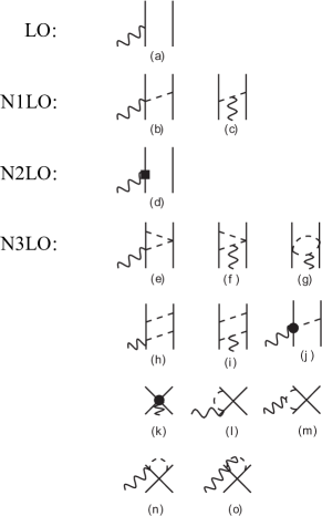
The contributions to the current operators up to one loop are illustrated diagrammatically in Fig. 16, where the NLO terms correspond to the power counting . The electromagnetic currents from LO, N1LO, and N2LO terms and from N3LO loop corrections depend only on the known parameters and (N1LO and N3LO), and the nucleon magnetic moments (LO and N2LO). Note that the LO and N1LO currents are the same as the conventional ones, while the N2LO current consists of relativistic corrections to the LO one. Unknown low-energy constants (LECs) enter the N3LO OPE contribution involving a vertex from a higher order chiral Lagrangian (proportional to the LECs ) and contact currents implied by nonminimal couplings Pastore et al. (2009); Piarulli et al. (2013). They are given by
| (118) | ||||
| (119) |
Before discussing the determination of these LECs, we note that the loop integrals in the N3LO diagrams of Fig. 16 are ultraviolet divergent and are regularized using dimensional regularization. The divergent parts of these loop integrals are reabsorbed by the LECs multiplying contact terms. Finally, the resulting renormalized electromagnetic operators have power-law behavior for large momenta, and must be further regularized before they can be sandwiched between nuclear wave functions. This is accomplished by the inclusion of a momentum-space cutoff of the type with in the range –700) MeV/c. The expectation is that observables, like magnetic moments and transitions in light nuclei are fairly insensitive to variations of in this range.
The , entering the OPE N3LO current, could be fitted to pion photo-production data on a single nucleon or related to hadronic coupling constants by resonance saturation arguments Pastore et al. (2009); Piarulli et al. (2013). Both procedures have drawbacks. While the former achieves consistency with the single-nucleon sector, it nevertheless relies on single-nucleon data involving photon energies much higher than those relevant to the threshold processes under consideration and real (in contrast to virtual) pions. The second procedure is questionable because of poor knowledge of some of the hadronic couplings, such as . Alternative strategies have been investigated for determining the LECs as well as and Piarulli et al. (2013). In this respect, it is convenient to define the dimensionless LECs (in units of the cutoff ) related to the original set via
| (120) |
where the superscript or on the characterizes the isospin of the associated operator.
The isoscalar and have been fixed by reproducing the experimental deuteron magnetic moment and isoscalar combination of the trinucleon magnetic moments. It turns out that in calculations based on the AV18 and AV18+UIX Hamiltonians the LEC multiplying the contact current assumes reasonable values, and 5.2 corresponding to MeV and 600 MeV, while the LEC values are quite small and –0.20 for the same range of cutoff Piarulli et al. (2013).
Three different strategies, referred to as I, II, and III, have been investigated to determine the isovector LECs , , and . In all cases I-III, is assumed as suggested by dominance in a resonance saturation picture of the N3LO OPE current of panel (j) in Fig. 16. In set I, and have been constrained to reproduce the experimental values of the radiative capture cross section at thermal neutron energies and the isovector combination of the trinucleon magnetic moments. This, however, leads to unreasonably large values for both LECs, and is clearly unacceptable Piarulli et al. (2013). In sets II and III, the LEC is fixed by assuming dominance while the LEC multiplying the contact current is fitted to reproduce either in set II or in set III. Both alternatives still lead to somewhat large values for this LEC: and –11.6 in set II and and –1.0 in set III. There are no three-body currents at N3LO Pastore et al. (2009), and therefore it is reasonable to fix the strength of the contact operators by fitting a observable such as and .
V.3 Elastic and inelastic form factors
The longitudinal and transverse form factors for elastic and inelastic transitions are extracted from electron scattering data by measuring the cross section Donnelly and Sick (1984)
| (121) |
where is the Mott cross section, and are the electron three- and four-momentum transfers, is the recoil correction , and are the electron initial energy and scattering angle in the laboratory, and is the mass of the target nucleus. In the case of elastic scattering, the electron energy transfer is and the four-momentum transfer . The form factors and are expressed in terms of reduced matrix elements (RMEs) of charge (), magnetic (), and electric () multipole operators, defined below, as
| (122) | ||||
| (123) |
We note that for elastic scattering and the RMEs vanish because of time reversal invariance.
Standard techniques Walecka (1995) are used to carry out the multipole expansion of the electromagnetic charge and current operators in a reference frame in which the axis defines the spin-quantization axis, and the direction is specified by the angles and :
| (124) | ||||
| (125) |
where , the are spherical harmonics, and the are rotation matrices Edmonds (1957). The unit vectors denote the linear combinations
| (126) |
with , , and . These relations are used below to isolate the contributing RMEs to elastic transitions in nuclei with . The ground states of nuclei in the mass range have spins ranging from (as in 12C) to (as in 10B), and are described by VMC or GFMC wave functions. For reasons of computational efficiency, it is convenient to determine the RMEs of charge and magnetic multipoles contributing to a specific transition by evaluating the matrix elements of and between states having a given spin projection , usually the stretched configuration with , for a number of different directions. The matrix element of the charge operator can then be written as
| (127) |
where is the angle that makes with the spin-quantization axis, the are Legendre polynomials, and is the Clebsch-Gordan coefficient . Generally, for a nucleus of spin the number of contributing (real) RMEs of charge multipole operators is (here denotes the integer part of ) and the allowed are the even integers between 0 and . Thus, it is possible to select independent directions, evaluate the matrix element of the charge operator for each of these different , and then determine the RMEs by solving a linear system. For example, for a nucleus of spin (like 6Li)
| (128) | ||||
| (129) |
where is a short-hand notation for .
For the transverse elastic form factor, it is possible to proceed in a similar fashion. Since electric multipoles do not contribute in elastic scattering
| (130) |
where the unit vectors , , have been defined in Eq. (126). Using the identity Edmonds (1957)
| (131) |
and, rather than considering the spherical components of the current, it is possible to work with its component along the unit vector defined earlier; further, can be taken in the -plane (), in which case is along the axis, leading to
| (132) |
where are associated Legendre functions. For a nucleus of spin , the number of contributing (purely imaginary) RMEs of magnetic multipole operators is , and the allowed are the odd integers between 0 and . In the case of a nucleus, for example, it is possible to take along the axis (), and determine from
| (133) |
Finally, the small behavior of the charge monopole and quadrupole, and magnetic dipole RMEs is given by:
| (134) | |||
| (135) | |||
| (136) |
where and are the quadrupole moment and magnetic moment, defined in terms of matrix elements of the charge and current density operators and respectively as
| (137) | |||||
| (138) |
They are determined by extrapolating to zero a polynomial fit (in powers of ) to the calculated and on a grid of small values. Consequently, the longitudinal form factor at is normalized as
| (139) |
while the transverse form factor vanishes at . Note that experimental data for are often reported in the literature as normalized to one at .
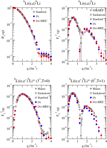
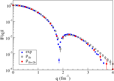
In QMC, matrix elements are evaluated as described in Sec. III.2.2. The results of elastic and inelastic electromagnetic form factors for 6Li are shown in Fig. 17. The calculations were performed within the impulse approximation (IA), and two-body operators added (IA+MEC). Overall, the agreement with the experimental data is excellent. The contribution of MEC is generally small but its inclusion improves the agreement between theory and data. In particular, it shifts the longitudinal elastic and inelastic form factors to slightly lower values, and sensibly increases the transverse inelastic form factor.
The longitudinal form factor of 12C is shown in Fig. 18. The calculation has been performed including only one-body operators (empty symbols), and one- plus two-body operators Lovato et al. (2013). The experimental data are from a compilation by Sick (2013, 1982), and are well reproduced by theory over the whole range of momentum transfers. The two-body contributions are negligible at low , and become appreciable only for fm-1, where they interfere destructively with the one-body contributions, bringing theory into closer agreement with experiment.
V.4 Second state of 12C: Hoyle state
The second state of 12C is the famous Hoyle state, the gateway for the triple-alpha burning reaction in stars. It is a particularly difficult state for shell model calculations as it is predominantly a four-particle four-hole state. However the flexible nature of the variational trial functions allows us to directly describe this aspect of the state.
To do this Pieper and Carlson (2015) two different types of single-particle wave functions have been used in the of Eq. (30): 1) the five conventional -coupled shell model states and 2) states that have an explicit three-alpha structure. The first alpha is in the shell, the second in the shell and the third in either the or shells. The latter can have four nucleons in or four in or two in and two in . In addition we allow the third alpha to have two nucleons in and two in (a two-particle two-hole excitation). This gives us a total of 11 components in ; a diagonalization gives the for the ground and excited states.
The resulting ground state has less than 1% of its in the shell while the second state has almost 70% in the shell. The GFMC propagation is then done for the first two states; the resulting energies are shown as a function of imaginary time in Fig. 19 which has results for two different initial sets of . The GFMC rapidly improves the variational energy and then produces stable (except for Monte Carlo fluctuations) results to large . The resulting ground state energy is very good, MeV versus the experimental value of MeV. However the Hoyle state excitation energy is somewhat too high, 10.4(5) versus 7.65 MeV.
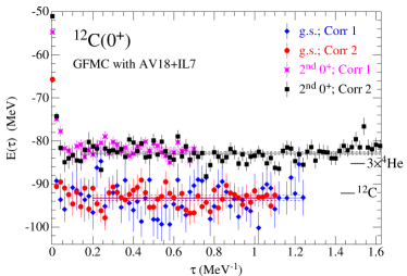
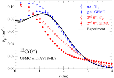
.
Figure 20 shows the resulting VMC and GFMC densities for one of the sets of . The GFMC propagation builds a dip at into the ground-state density which results in good agreement with the experimental value. However the Hoyle-state density is peaked at in both the VMC and GFMC calculations. A possible interpretation of these results is that the ground state is dominated by an approximately equilateral distribution of alphas while the Hoyle state has an approximately linear distribution.
The calculated impulse transition form factor is compared to the experimental data in Fig. 21. The insert is scaled such that (linear) extrapolation to gives the . The GFMC more than doubles the VMC result and gives excellent agreement with the data.
V.5 Magnetic moments and electroweak transitions
In the impulse approximation (IA), magnetic moments are calculated as
| (140) |
where , , , and and are the isoscalar and isovector combinations of the anomalous magnetic moment of the proton and neutron. The magnetic moment corrections associated with the two-body operators discussed in the previous sections are obtained from diagonal nuclear matrix elements
| (141) |
where the nuclear wave function is taken with , the momentum transfer is taken along , is the nucleon mass, and the extrapolation to determine is done from calculations performed at several small values of .
The total magnetic moments, including MEC derived within EFT, have been presented in Table 1 of Sec. IV.1. Results obtained using MEC derived in the conventional approach and within EFT are very similar, and have been discussed in detail in Pastore et al. (2013). Here it is interesting to discuss the role of MEC compared to the IA. GFMC calculations using AV18+IL7 and chiral two-body currents of the magnetic moments are shown in Fig. 22. The experimental magnetic moments of nuclei were used to constrain the LECs of the EFT; all the results for heavier nuclei are predictions.
In many cases the two-body currents significantly change the IA results and in all of these much better agreement with experiment is achieved. The contribution of MEC is generally larger for even-odd and odd-even nuclei, in particular for 9Li and 9C. The exceptions are 9Be and 9B, which with their [441] spatial symmetry are essentially single nucleons outside a 8Be( core; on average, these have no OPE interaction with the core and therefore no significant MEC contribution. For odd-odd isoscalar nuclei, the IA results are already in good agreement with experimental data; only for the nuclei 8Li and 8B are the MEC contributions significant.
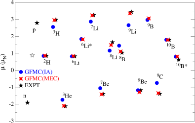
and electromagnetic transitions for =6–9 nuclei have been calculated with GFMC. The one-body part of these operators are given by
| (142) |
where is a spherical harmonic, and the orbital and spin angular momentum operators, and and the gyromagnetic ratio of protons and neutrons. MEC are also included in the transitions. The nuclear matrix elements can be compared with the experimental widths. In units of MeV, they are given by Preston (1962)
| (143) |
where is the energy difference between the final and initial state and is in units of and is in units of fm4.
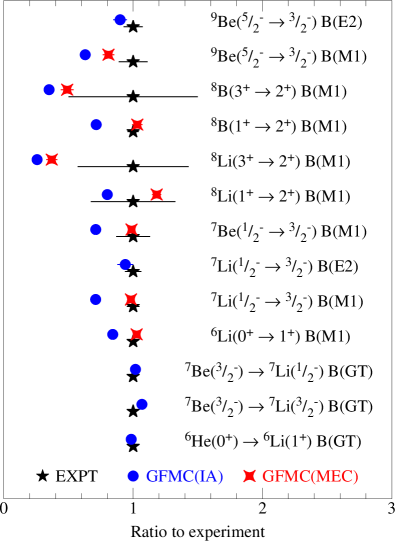
A number of calculated electromagnetic transition strengths are compared to experiment in Fig. 23. Many additional transitions within 8Be are reported in Pastore et al. (2014). Again GFMC calculations were made using AV18+IL7 and chiral two-body currents. The two-body currents make large corrections to the IA results for the transitions; these often result in excellent agreement with experiment.
Weak decays of =6, 7 nuclei have been evaluated using QMC but much more needs to be done in the future. In IA, the weak Fermi (F) and Gamow-Teller (GT) operators to be evaluated are:
| (144) |
A first calculation for the weak decays 6HeLi and 7BeLi was made by Schiavilla and Wiringa (2002) using VMC wave functions for the AV18+UIX Hamiltonian, and incorporating conventional MEC as discussed in Sec. V.1.2. Parameters in the MEC were fixed to reproduce 3H -decay Schiavilla et al. (1998).
The 6He -decay is a pure GT transition, while the 7Be electron capture is a mixed F+GT transition to the ground state, and a GT transition to the first excited state of 7Li. These are superallowed decays where the dominant spatial symmetry of the parent and daughter states is the same, e.g., [42][42] in =6 and [43][43] in =7. In these cases, the F and GT matrix elements are of order 1–2 and the MEC contributions are only a 2–4% correction.
Subsequently, a GFMC calculation for these transitions was made by Pervin et al. (2007) based on the AV18+IL2 Hamiltonian, but only in the IA. The GFMC results for these three B(GT) reduced transition probabilities are shown at the bottom of Fig. 23. These are already in fairly good agreement with experiment, and small MEC corrections will not shift the results by much.
Weak decays in the =8,9 nuclei pose a much bigger challenge. For example, 8HeLi goes from a predominantly [422] symmetry state to multiple excited states, but primarily to the first excited state in 8Li. The latter is predominantly a [431] symmetry state with only a small [422] component, so the allowed GT matrix element is of order 0.1–0.2. Similarly, the 8LiBe and 8BBe decays are transitions from large to small components, with the added complication that the final state in 8Be is a moderately broad resonant state. GFMC calculations in impulse approximation underpredict the =8 experimental matrix elements by a factor of two Pastore (2014). It is possible that GFMC does an inadequate job of accurately determining small components in the final state wave functions, or that the specific Hamiltonian does not induce the required correlations. However, if the magnitude of the MEC corrections is comparable to that in the =6,7 superallowed decays, then the MEC will be relatively much more important in the allowed decays and may resolve the problem. This is an important task for future QMC studies.
V.6 Electroweak Response of Light Nuclei
The response to electroweak probes provides direct information on dynamics in the nucleus. The rich structure of nuclear interactions and currents, combined with the availability of different probes, offers the opportunity to study many intriguing aspects of nuclear dynamics. Here we describe theoretical approaches for describing inclusive scattering of electrons and neutrinos from a nucleus, including both sum-rule techniques and direct computations of response functions, as well as comparisons to available experimental data. In the last few years inclusive neutrino scattering from nuclear targets has seen a surge in interest, spurred by the excess, at relatively low energy, of measured cross section relative to theoretical calculations observed in recent neutrino quasi-elastic scattering data on 12C Aguilar-Areval (2008); Butkevich (2010). Analyses based on these calculations have led to speculations that our present understanding of the nuclear response to charge-changing weak probes may be incomplete Benhar et al. (2010). However, it should be emphasized that the calculations on which these analyses are based use rather crude models of nuclear structure—Fermi gas or local density approximations of the nuclear matter spectral function—and simplistic treatments of the reaction mechanism, and should therefore be viewed with some skepticism. The differential cross section for neutrino and antineutrino inclusive scattering off a nucleus, specifically the processes and induced by neutral weak currents (NC), and the processes and induced by charge-changing weak currents (CC), can be expressed in terms of five response functions as
| (145) |
where = for the NC processes and = for the CC processes, and the () sign in the last term is relative to the () initiated reactions. The value of is GeV-2 as obtained from an analysis of super-allowed -decays by Towner and Hardy (1999)—this value includes radiative corrections—while is taken as 0.97425 from Nakamura (2010). The initial neutrino four-momentum is , the final lepton four momentum is , and the lepton scattering angle is denoted by . The lepton energy and momentum transfers are defined as and , respectively, and the squared four-momentum transfer as . The Fermi function accounts for the Coulomb distortion of the final lepton wave function in the charge-raising reaction,
| (146) |
with
| (147) |
otherwise it is set to one. Here , is the gamma function, is the nuclear radius, and is the fine structure constant. There are in principle radiative corrections for the CC and NC processes due to bremsstrahlung and virtual photon- and -exchanges. These corrections have been evaluated in the deuteron by Towner and Hardy (1998), and Kurylov et al. (2002) at the low energies ( MeV) relevant for the SNO experiment, which measured the neutrino flux from the 8B decay in the sun. They are not considered further below, since our focus here is primarily on scattering of neutrinos with energies larger than 100 MeV, and we are not concerned with discussing cross section calculations with % accuracy in this regime. The nuclear response functions are defined as
| (148) | |||||
| (149) | |||||
| (150) | |||||
| (151) | |||||
| (152) | |||||
where represents the initial ground state of the nucleus of energy , its final state of energy , and an average over the initial spin projections is understood. The three-momentum transfer is taken along the -axis (i.e., the spin-quantization axis), and is the time component (for ) or space component (for ) of the NC or CC. Note that in the model of electroweak currents adopted here, their -dependence enters through the dependence on of the electroweak form factors of the nucleon and -to- transition. Below, when discussing QMC calculations of , the four-momentum transfer is fixed at the top of the quasi-elastic peak, and the form factors are evaluated at with , so that the only -dependence left in is that from the energy-conserving -function.
The expression above for the CC cross section is valid in the limit , in which the lepton rest mass is neglected. At small incident neutrino energy, this approximation is not correct. Inclusion of the lepton rest mass leads to changes in the kinematical factors multiplying the various response functions. The resulting cross section can be found in Shen et al. (2012).
The cross section for inclusive electron scattering follows from Eq. (145) by using current conservation to relate the longitudinal component of the current to the charge operator via and by noting that the interference response vanishes, since it involves matrix elements of the vector and axial parts of the current or of the type . One finds
| (153) |
where is the Mott cross section, and the longitudinal () and transverse () response functions are defined as in Eqs. (148) and (151) with replaced by .
The accurate calculation of the inclusive response at low and intermediate energy and momentum transfers (say, GeV/c and in the quasi-elastic region) is a challenging quantum many-body problem, since it requires knowledge of the whole excitation spectrum of the nucleus and inclusion in the electroweak currents of one- and two-body terms. In the specific case of inclusive weak scattering, its difficulty is compounded by the fact that the energy of the incoming neutrinos is not known (in contrast to inclusive scattering where the initial and final electron energies are precisely known). The observed cross section for a given energy and angle of the final lepton results from a folding with the energy distribution of the incoming neutrino flux and, consequently, may include contributions from energy- and momentum-transfer regions of the nuclear response where different mechanisms are at play: the threshold region, where the structure of the low-lying energy spectrum and collective effects are important; the quasi-elastic region, which is dominated by scattering off individual nucleons and nucleon pairs; and the resonance region, where one or more pions are produced in the final state.
The simplest model of nuclear response is based on the plane-wave impulse approximation (PWIA). The response is assumed to be given by an incoherent sum of scattering processes off single nucleons that propagate freely in the final state. In PWIA the struck nucleon with initial momentum absorbs the momentum of the external field and transitions to a free particle state of momentum without suffering any interactions with the residual system. In the most naive formulation of PWIA, the response is obtained from the single-nucleon momentum distribution in the ground-state of the nucleus and the nucleon electroweak form factors,
| (154) |
where describes the coupling to the external electroweak field, is the nucleon momentum distribution, and the effects of nuclear interactions are subsumed in the single parameter , which can be interpreted as an average binding energy. The remaining terms in the -function are the final energies of the struck nucleon and recoiling system, respectively. In cases where the momentum transfer is large, it may be more appropriate to use relativistic expressions for the coupling and final nucleon kinetic energy.
More sophisticated formulations of PWIA are based on the spectral function, thus removing the need for including the parameter . To this end, it is useful to first express the response in terms of the real-time propagation of the final state as
| (155) |
where the ’s denote the relevant components of the electroweak current of interest. Since the interactions of the struck nucleon with the remaining nucleons are neglected, the -body Hamiltonian reduces to , where is the kinetic energy operator of nucleon (the struck nucleon) and is the Hamiltonian for the remaining (and fully interacting) nucleons.
Ignoring the energy dependence in the spectral function reproduces the naive PWIA response, since integrating the spectral function recovers the momentum distribution. At large values of the momentum transfer ( GeV/c), one would expect the spectral function approach to be reasonably accurate. There will be significant corrections, however, arising from the fact that in some instances the struck nucleon is not only in a mean field, but is strongly interacting with one or more other nucleons. More sophisticated treatments are required to get a complete picture.
PWIA calculations of the longitudinal response measured in scattering, for example, grossly overestimate the data in the quasi-elastic peak region Carlson and Schiavilla (1998). They also lead to an incorrect strength distribution, since they underestimate energy-weighted sum rules of the longitudinal (and transverse) response functions. Much of this overestimate can be attributed to the fact the charge can propagate through the interaction, not only through the movement of nucleons.
It is possible to compute sum rules of the electroweak response as ground state expectation values that are much more accurate than approximations to the full response. One can also calculate integral transforms of the response, which can be directly compared to experimental data and provide a great deal of information about the full response. Here we review results for sum rules and Euclidean response.
V.7 Sum rules of electroweak response functions
Sum rules provide a powerful tool for studying integral properties of the response of a nuclear many-body system to an external probe. Of particular interest are those at constant three-momentum transfer, since they can be expressed as ground-state expectation values of appropriate combinations of the electroweak current operators (and commutators of these combinations with the Hamiltonian in the energy-weighted case), thus avoiding the need for computing the nuclear excitation spectrum.
In the electromagnetic case, the (non-energy-weighted) sum rules are defined as Carlson et al. (2002)
| (156) |
where is the longitudinal () or transverse () response function, is the energy transfer corresponding to the inelastic threshold, is the proton electric form factor (evaluated at four-momentum transfer ), and the ’s are appropriate normalization factors, given by
| (157) |
Here () and () are the proton (neutron) number and magnetic moment, respectively. These factors have been introduced so that under the approximation that the nuclear electromagnetic charge and current operators originate solely from the charge and spin magnetization of individual protons and neutrons and that relativistic corrections to these one-body operators—such as the Darwin-Foldy and spin-orbit terms in the charge operator—are ignored. The sum rules above can be expressed McVoy and Van Hove (1962) as ground-state expectation values of the type
| (158) |
where is either the charge () or transverse current () operator divided by , denotes the ground state of the nucleus recoiling with total momentum , and an average over the spin projections is understood. The as defined in Eq. (156) only includes the inelastic contribution to , i.e., the elastic contribution represented by the second term on the r.h.s. of Eq. (158) has been removed. It is proportional to the square of the longitudinal or transverse elastic form factor. For states like 4He or 12C, vanishes, while , discussed in Sec.V.2 is given by , with the four-momentum transfer and corresponding to elastic scattering, ( is the rest mass of the nucleus).
In the case of NC and CC weak response functions, the (non-energy-weighted) sum rules are generally defined as Lovato et al. (2014)
| (159) |
and can be expressed as
| (160) | ||||
| (161) |
where the ’s are convenient normalization factors (see below), , , , and , and for the expectation value of is computed. Note that the electroweak nucleon and -to- form factors in are taken to be functions of only by evaluating them at , at the top of the quasi-elastic peak. In contrast to the electromagnetic sum rules above, the include the elastic and inelastic contributions; the former are proportional to the square of electroweak form factors of the nucleus. In the large limit, these nuclear form factors decrease rapidly with , and the sum rules reduce to the incoherent sum of single-nucleon contributions. The normalization factors are chosen such that , for example
| (162) |
where () is the proton (neutron) number, is the weak axial form factor of the nucleon normalized as , and and are its weak vector form factors. The and are the ordinary proton and neutron magnetic form factors, normalized to the proton and neutron magnetic moments: and . Thus the give sum rules of response functions corresponding to approximately point-like electroweak couplings.
Obviously, sum rules of weak response functions cannot be compared to experimental data. Even in the electromagnetic case, a direct comparison between the calculated and experimentally extracted sum rules cannot be made unambiguously for two reasons. First, the experimental determination of requires measuring the associated in the whole energy-transfer region, from threshold up to . Inclusive electron scattering experiments only allow access to the space-like region of the four-momentum transfer (). While the response in the time-like region () could, in principle, be measured via annihilation, no such experiments have been carried out to date. Therefore, for a meaningful comparison between theory and experiment, one needs to estimate the strength outside the region covered by the experiment. In the past this has been accomplished in the case of either by extrapolating the data Jourdan (1996) or, in the few-nucleon systems, by parametrizing the high-energy tail and using energy-weighted sum rules to constrain it Schiavilla et al. (1989, 1993).
The second reason that direct comparison of theoretical and “experimental” sum rules is difficult lies in the inherent inadequacy of the dynamical framework adopted in this review to account for explicit pion production mechanisms. The latter mostly affect the transverse response and make its -peak region outside the range of applicability of this approach. At low and intermediate momentum transfers ( MeV/c), the quasi-elastic and -peak are well separated, and it is therefore reasonable to study sum rules of the electromagnetic transverse response. In the quasi-elastic region, where nucleon and (virtual) pion degrees of freedom are expected to be dominant, the dynamical framework adopted in the present review should provide a realistic and quantitative description of electromagnetic (and weak) response functions.
In Figs. 24 and 25, we show recent results obtained for the electromagnetic longitudinal and transverse sum rules in 12C. The open squares give the experimental sum rules and obtained by integrating up to (in the region where measurements are available) the longitudinal and transverse response functions (divided by the square of ) extracted from world data on inclusive scattering off 12C Jourdan (1996); see Lovato et al. (2013) for additional details. We also show by the solid squares the experimental sum rules obtained by estimating the contribution of strength in the region . This estimate is made by assuming that for , i.e., well beyond the quasi-elastic peak, the longitudinal or transverse response in a nucleus like 12C () is proportional to that in the deuteron (), which can be accurately calculated Shen et al. (2012). This scaling assumes that the high-energy part of the response is dominated by physics, and that the most important contribution is from deuteron-like pairs. It is consistent with the notion that at short times the full propagator is governed by the product of pair propagators (assuming interactions are weak), discussed earlier in Sec.V.6. Thus, one sets , and determines by matching the experimental 12C response to the calculated deuteron one. It is worthwhile emphasizing that, for the transverse case, this estimate is particularly uncertain for the reasons explained earlier; the data on Jourdan (1996) indicate that at the higher values for there might be already significant strength that has leaked in from the -peak region.
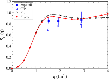
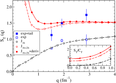
The sum rules computed with the AV18+IL7 Hamiltonian and one-body only or one- and two-body terms in the electromagnetic charge and current operators are shown, respectively, by the dashed and solid lines in Figs. 24–25. In the small limit, vanishes quadratically, while the divergent behavior in is due to the present in the normalization factor . In this limit, Carlson and Schiavilla (1998); Marcucci et al. (2005), where is the Hamiltonian and is the proton projector, and therefore is finite; the associated strength is due to collective excitations of electric-dipole type in the nucleus. In the large- limit, the one-body sum rules differ from unity because of relativistic corrections in , primarily the Darwin-Foldy term which gives a contribution to , where , and because of the convection term in , which gives a contribution to , where is the proton kinetic energy in the nucleus.
In contrast to , the transverse sum rule has large two-body contributions. This is consistent with studies of Euclidean transverse response functions in the few-nucleon systems Carlson et al. (2002), which suggest that a significant portion of this excess transverse strength is in the quasi-elastic region. Overall, the calculated and are in reasonable agreement with data. However, a direct calculation of the response functions is clearly needed for a more meaningful comparison between theory and experiment.
While sum rules of NC or CC weak sum rules are of a more theoretical interest, they nevertheless provide useful insights into the nature of the strength seen in the quasi-elastic region of the response and, in particular, into the role of two-body terms in the electroweak current. Those corresponding to weak NC response functions and relative to 12C are shown in Fig. 26: results () corresponding to one-body (one- and two-body) terms in the NC are indicated by the dashed (solid) lines. Note that both and are normalized by the same factor , which makes in the large limit. In the small limit, and are much larger than for .
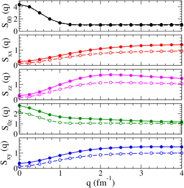
Except for , the sum rules are considerably larger than the , by as much as 30-40%. This enhancement is not seen in calculations of neutrino-deuteron scattering Shen et al. (2012). The increase due to two-body currents is quite substantial even down to small momentum transfers. At , the enhancement is about 50% relative to the one-body values. In general, the additional contributions of the two-body currents () to the sum rules are given by a combination of interference with one-body currents (), matrix elements of the type , and contributions of the type . At low momentum transfers the dominant contributions are found to be of the latter type, where the same pair is contributing in both left and right operators. Enhancements of the response due to two-body currents could be important in astrophysical settings, where the neutrino energies typically range up to 50 MeV. A direct calculation of the 12C response functions is required to determine whether the strength of the response at low extends to the low energies kinematically accessible to astrophysical neutrinos.
At higher momentum transfers the interference between one- and two-body currents plays a more important role. The larger momentum transfer in the single-nucleon current connects the low-momentum components of the ground-state wave function directly with the high-momentum ones through the two-body current. For nearly the same Hamiltonian as is used here, there is a 10% probability that the nucleons have momenta greater than 2 fm-1 implying that of the wave function amplitude is in these high-momentum components Wiringa et al. (2014). The contribution of pairs remains dominant at high momentum transfers, and matrix elements of the type + c.c. at short distances between nucleons and are critical.
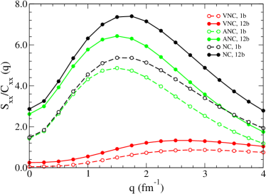
Figure 27 shows the separate contributions associated with the vector (VNC) and axial-vector (ANC) parts of the sum rule. The ANC piece of the sum rule is found to have large two-body contributions of the order of 30% relative to the one-body part. Similar results are found for the and sum rules; the sum rule is nonzero because of interference between the VNC and ANC and vanishes in the limit in which only one or the other is considered. The ANC two-body contributions in the sum rules are much larger than the contributions associated with axial two-body currents in weak charge-changing transitions to specific states at low-momentum transfers, such as -decays and electron- and muon-capture processes involving nuclei with mass numbers =3–7 Marcucci et al. (2011); Schiavilla and Wiringa (2002), where they amount to a few % (but are nevertheless necessary to reproduce the empirical data).
In summary, two-body currents generate a significant enhancement of the single-nucleon neutral weak current response, even at quasi-elastic kinematics. This enhancement is driven by strongly correlated pairs in nuclei. The presence of these correlated pairs also leads to important interference effects between the amplitudes associated with one- and two-body currents: the single-nucleon current can knock out two particles from a correlated ground state, and the resulting amplitude interferes with the amplitude induced by the action of the two-body current on this correlated ground state.
V.8 Euclidean response functions
Direct calculations of are difficult in systems with , and at the moment one has to rely on techniques based on integral transforms relative to the energy transfer, which eliminate the need for summing explicitly over the final states. Two such approaches have been developed: one based on the Lorentz-integral transform (LIT) has been used extensively in the few-nucleon systems, albeit so far by including only one-body electroweak current operators. It has been reviewed recently Leidemann and Orlandini (2013), and will not be discussed here. The other approach is based on the Laplace transform Carlson and Schiavilla (1992, 1994) and leads to Euclidean (or imaginary time) response functions, defined as
| (163) |
The Euclidean response is essentially a statistical mechanical formulation, and hence can be evaluated with QMC methods similar to those discussed earlier. Electromagnetic Euclidean response functions have been calculated for the few-nucleon systems (=3 and 4) Carlson and Schiavilla (1992, 1994); Carlson et al. (2002), and very recently for 12C Lovato et al. (2015). It should be realized that in a nucleus like 12C these are very computationally intensive calculations, requiring tens of millions of core hours on modern machines.
In the case of scattering the electromagnetic Euclidean response functions can be compared directly with experimental data, by simply evaluating the Laplace transforms of the measured response functions, at least for values of large enough so as to make mostly sensitive to strength in the quasi-elastic and low-energy regions of .
The response at is identical to the sum rule, and its slope at is equivalent to the energy-weighted sum rule. The simulation proceeds by calculating the ground-state wave function using GFMC, and then evaluating the imaginary-time dependent correlation functions over a range of separations using the same paths sampled in the original ground-state calculation. Since the current operators couple to states of different spin and isospin, the calculations require recomputing the path integral for different current operators .
To more easily compare the Euclidean response to data for larger , we multiply by a scaling factor . For a free nucleon initially at rest, this scaled response is a constant independent of , since the response is a delta function in energy for each momentum transfer . The slope and curvature of the calculated Euclidean response at low indicates the strength at high energy, and the response at large is related to the low-energy part of the nuclear response. The calculated responses have a higher average energy than simple PWIA-like approaches, and also have greater strength at high energy (from processes) and at low energy (from low-lying nuclear states).
The difference between the full response and the simple PWIA is most easily understood for the longitudinal response, which is dominated by one-nucleon currents. The PWIA is sensitive to the momentum distribution of the protons, as it assumes that the struck nucleon does not interact with other nucleons. The full calculation is also sensitive to the propagation of charge through the NN interaction, since the struck proton can charge exchange with other nucleons. This rapid propagation of charge leads to an enhanced strength at high energy.
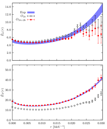
In Fig. 28 we show recent calculations Lovato et al. (2015) of the 12C Euclidean electromagnetic longitudinal and transverse response compared with experimental data. The overall agreement with experiment in the longitudinal channel is excellent. Here the calculation with the full currents is very similar to that with one-nucleon currents alone. The error bars are higher at large (lower energy) because of the required subtraction of the elastic contribution.
The transverse response is shown in the lower panel of Fig. 28. The difference between single-nucleon currents and one- plus two-nucleon currents is quite substantial and extends over the full range of . This implies a substantial enhancement of the cross section in the full energy region, including both the quasi-elastic peak and the low-energy regime. The full calculation is in good agreement with experiment. The enhancement can in some cases be as large as 40%, somewhat larger than typical effects of two-nucleon currents on the squared matrix elements of low energy transitions, but not dramatically so. The larger momentum transfers in these inclusive experiments can be expected to lead to larger contributions from pion- and currents, and these are found to be the dominant two-nucleon current contributions.
Ideally one would like to invert the Laplace transform to obtain a more direct reconstruction of the response as a function of momentum and energy transfer. This has been accomplished already for A=4, where the calculations are much faster and hence the simulations can be carried out with high accuracy. Recent calculations Lovato et al. (2015) agree with earlier calculations of the EM response of 4He Carlson et al. (2002), but the statistical accuracy is at least an order of magnitude better.
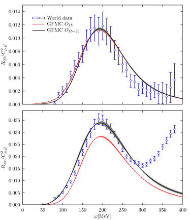
For such accurate data the maximum entropy method Bryan (1990); Jarrell and Gubernatis (1996) can be used to reconstruct the response. Results for 4He at q=600 MeV/c are shown in Fig. 29, similar accuracy is obtained over a wide range of momentum transfers. Again it is seen that the enhancement from two nucleon currents is substantial and extends over the whole quasielastic regime. At higher energies the calculated response does not include pion production and hence fails to reproduce the strength associated with production.
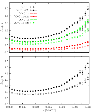
Imaginary time response functions for the neutral current response of 12C have also been performed Lovato et al. (2015) and are shown in Fig. 30. At present the statistical accuracy is not sufficient to invert the response, but the Euclidean response already gives important results. These calculations demonstrate an enhancement of the axial currents in addition to the expected enhancement in the vector channels. In particular, the vector-axial interference response (lower panel) is significantly enhanced by the two-nucleon currents. It is this response that gives the difference between neutrino and anti-neutrino cross sections. This is a very important quantity in attempts to isolate the CP-violating phase in the neutrino sector or the mass hierarchy in long-baseline experiments; see for example LBNE Collaboration et al. (2013). Future work on charge current responses and inversions to the real-time response have many important applications including accelerator neutrinos and neutrinos in astrophysical environments.
VI The equation of state of neutron matter
VI.1 Pure neutron matter: Homogeneous phase
The equation of state (EoS) of neutron matter is a key ingredient in understanding the static and dynamic properties of neutron stars. In the region between the inner crust and the outer core, neutron stars are primarily neutrons, in equilibrium with a small fraction of protons, electrons and muons in -decay equilibrium. It has been argued that when the chemical potential is large enough, heavier particles containing strange quarks may appear. This is expected to happen at densities Lonardoni et al. (2015). However, while the determination of the maximum mass of neutron stars requires knowledge of the EoS up to several times nuclear densities, the EoS around nuclear density and up to about largely determines their radii Lattimer and Prakash (2001). Astrophysical applications are not the only relevant ones. The EoS of neutron matter is used to constrain effective forces in the presence of large isospin-asymmetry. For example, the bulk term of Skyrme models is sometimes fitted with input from a neutron matter EoS.
Neutron matter is not directly accessible in terrestrial experiments, and all the indirect experimental evidence related to it is based on extrapolations of measurements on heavy nuclei, and on astrophysical observations (see, e.g., Danielewicz et al. (2002)). The role of ab-initio techniques becomes therefore crucial as a tool for testing the model Hamiltonians that can be directly fitted on experimental data for light nuclei against the constraints deriving from indirect measurements.
At low densities fm-3 properties of neutron matter are very similar to ultra-cold Fermi gases that have been extensively studied in experiments. In this regime, the interaction is mainly s-wave, and the system strongly paired. The nuclear interaction can be simplified, the standard DMC method for central potentials can be used, and very accurate results for the energy and the pairing gap obtained Gezerlis and Carlson (2008, 2010); Carlson et al. (2012). Other results obtained using AFDMC with the full nuclear Hamiltonian are qualitatively similar Gandolfi et al. (2008a, 2009a). At higher densities, the contribution of higher partial waves becomes important, and the complete nuclear Hamiltonian has to be used to calculate the EoS.
Argonne and other modern interactions are very well suited to study dense matter. The scattering data are described well with AV18 in a very wide range of laboratory energies, and this gives an idea to their validity to study dense matter. A laboratory energy of 350 MeV (600 MeV) corresponds to a Fermi momentum k400 MeV (530 MeV) and to a neutron density (). This is not the case of softer potentials fitted to very low energy scattering data. The AV18 and AV8′ two-body interactions combined with the UIX three-body force have been extensively employed to calculate the properties of neutron matter and its consequences for neutron star structure (see, e.g., Akmal et al. (1998)). In the past, several attempts to use Illinois three-body forces were made, but they provided unexpected overbinding of neutron matter at large densities Sarsa et al. (2003), and will not be discussed any further. It has been recently shown that even the IL7 three-body interaction gives an EoS too soft Maris et al. (2013). It would be very interesting to calculate the EoS of symmetric nuclear matter using IL7, but unfortunately there are no such calculations.
The first AFDMC calculations of the EoS of neutron matter including three-body forces has been produced by Sarsa et al. (2003). Later using a different implementation of the constrained-path and with more statistics, better agreement was obtained with GFMC where the comparison is available Gandolfi et al. (2009b). To date, only the equation of state of pure neutron matter has been calculated with QMC using realistic Hamiltonians, while nuclear matter can be studied by including only two-body forces Gandolfi et al. (2014).
By imposing periodic boundary conditions it is possible to simulate an infinite system using a finite number of particles. However, the energy and other physical quantities are affected by the spatial cut-offs that are required to make the wave function compatible with periodic boundary conditions. The effect of cutting the potential energy at the edge of the simulation box is made milder by summing the contributions due to periodic images of the nucleons included in a given number of shells of neighboring image simulation cells. Finite size corrections to the kinetic energy already appear for the Fermi gas. In order to have a wave function that describes a system with zero total momentum and zero angular momentum, it is necessary to fill up a shell characterized by the modulus of the single particle momentum. This fact determines a set of magic numbers, which are commonly employed in simulations of periodic systems. The kinetic energy corresponding to each magic number is a non-regular and non-monotonic function of the number of Fermions Ceperley et al. (1977). This fact suggests that for an interacting system it is necessary to proceed with an accurate determination of the closed shell energies in order to minimize the discrepancy with the infinite system limit.
To this end, the effect of using different number of neutrons was carefully studied by means of the Periodic Box Fermi hypernetted chain (FHNC) method Fantoni and Schmidt (2001). This study showed that the particular choice of 33 Fermions (for each spin state) is the closest to the thermodynamic limit. Another strategy for allowing an accurate extrapolation consists of using the Twisted Averaged Boundary Conditions. The method, described in Lin et al. (2001) is based on randomly drifting the center of the Fermi sphere, which adds a phase to the plane waves used in the Slater determinant, in order to add contributions from wave vectors other than those strictly compatible with the simulation box. This procedure smooths the behavior of the energy as a function of , giving the possibility of better determining the limit Gandolfi et al. (2009b).
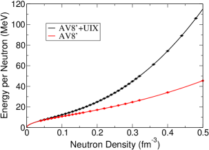
In Fig. 31 the EoS of neutron matter computed by a simulation with is presented. In order to check the consistency of the results given by AFDMC, a simulation was performed using only neutrons and by imposing the same boundary conditions to the interaction as in the GFMC calculation Carlson et al. (2003b); Carlson (2003). The comparison shows that the two methods are in good agreement Gandolfi et al. (2009b). Particular care was taken in studying the effect of finite-size effects by repeating each simulation using a different number of neutrons and using Twisted Averaged Boundary Conditions. The repulsive nature of the three-neutron interaction is clear from the figure, where the EoS obtained with and without UIX is shown.
The AFDMC results are conveniently fitted using the functional form
| (164) |
where is the energy per neutron (in MeV) as a function of the density (in fm-3). The parameters of the fit for both AV8′ and the full AV8′+UIX Hamiltonian are reported in Table 6.
| force | ||||||
|---|---|---|---|---|---|---|
| (MeV) | (MeV) | (MeV) | (MeV) | |||
| none | 30.5 | 31.3 | 12.7 | 0.49 | 1.78 | 2.26 |
| 32.1 | 40.8 | 12.7 | 0.48 | 3.45 | 2.12 | |
| 32.0 | 40.6 | 12.8 | 0.488 | 3.19 | 2.20 | |
| 32.0 | 44.0 | 13.0 | 0.49 | 3.21 | 2.47 | |
| 33.7 | 51.5 | 12.6 | 0.475 | 5.16 | 2.12 | |
| 33.8 | 56.2 | 13.0 | 0.50 | 4.71 | 2.49 | |
| UIX | 35.1 | 63.6 | 13.4 | 0.514 | 5.62 | 2.436 |
The EoS of neutron matter up to has been recently calculated by Gezerlis et al. (2013, 2014) with nuclear two-body local interactions derived within the chiral effective field theory. The AFDMC calculations for the EFT interaction at LO, NLO, and N2LO orders are shown in Fig. 32. (Note that three-body forces have not been included at N2LO). At each order in the chiral expansion, it is important to address the systematic uncertainties entering through the regulators used to renormalize short-range correlations; see Gezerlis et al. (2014) for more comprehensive details. In the figure, the EoS obtained using cutoffs of R0=1.0 fm and 1.2 fm are indicated. The figure shows that the results are converging in the chiral expansion, i.e. the energy per neutron at N2LO is quite similar to NLO. The three-neutron interaction entering at N2LO has not been included in the calculation but its contribution is expected to be small Tews et al. (2015). Other approaches based on lattice-based QMC methods have been explored recently by Wlazłowski et al. (2014) and Roggero et al. (2014), with very similar results also included in Fig. 32.
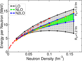
VI.1.1 Three-neutron force and Symmetry energy
As described in Sec. II.1 the force is obtained by accurately fitting scattering data, but a force is essential to have a good description of the ground states of light nuclei. The effect of the force on the nuclear matter EoS is particularly important, as it is needed to correctly reproduce the saturation density and the energy. The neutron matter EoS is also sensitive to the particular choice of the force, and consequently the corresponding neutron star structure.
By assuming that the Hamiltonian is well constrained by scattering data, the effect of using different three-neutron forces to compute the EoS of neutron matter has been studied carefully. As described in Sec. II.2 the force can be split into different parts: a long-range term given by -exchange, an intermediate part described by -rings and a phenomenological short-range repulsion. The role of the latter term is the least understood, although in part it is probably mocking up a relativistic boost correction to the interaction Akmal et al. (1998); Pieper et al. (2001). It is important to address the effect of all these terms in the calculation of neutron matter. These parts have been tuned and the effective range of the repulsive term changed to explore how these terms change the many-body correlations in neutron matter. The main part that has been explored is the short-range term. This term is purely phenomenological and it is mainly responsible for providing the correlations at high densities. The expectation value of the -exchange Fujita-Miyazawa operator in neutron matter is small compared to , and this limits almost the whole effect of UIX to the short-range term Gandolfi et al. (2012).
From the experimental side, the EoS of neutron matter cannot be measured, but strong efforts have been made to measure the isospin-symmetry energy, see the review by Tsang et al. (2012). By assuming a quadratic dependence of the isospin-asymmetry , the symmetry energy can be interpreted as the difference between pure neutron matter () and symmetric nuclear matter ()
| (165) |
where is the energy per neutron of pure neutron matter, and is the energy per nucleon of symmetric nuclear matter. The total energy of nuclear matter will take the form
| (166) |
Several experiments aim to measure the symmetry energy at the empirical saturation density =0.16 fm-3, and the parameter related to its first derivative. Around the symmetry energy can be expanded as
| (167) |
The present experimental constraints to have been used to study the sensitivity of the EoS of neutron matter to the particular choice of the force. The assumptions are that the empirical energy of nuclear matter at saturation is MeV, and through Eq. (165) there is a consequent range of the energy of neutron matter at saturation, . By following Tsang et al. (2009) the symmetry energy is expected to be in the range MeV, corresponding to the neutron matter energy MeV. Other papers report a wider range of values of ; see for example Chen et al. (2010).
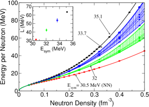
Following Pieper et al. (2001), different parametrizations of , and have been considered. Starting with the original strengths of these parameters, the constant has been adjusted in order to reproduce a particular value of and give a corresponding symmetry energy. We show the various EoS computed using different models of interactions in Fig. 33, compared to the AV8′ force alone and with the original UIX force. The blue and green bands in the figure show the EoS with a symmetry energy corresponding to 33.7 and 32 MeV, respectively. Each band covers the various results obtained using different three-neutron forces adjusted to have the same . The parameters fitting the higher and the lower EoS for each band are reported in Table 6. It is interesting to note that the bands are tiny around , and the uncertainty grows at larger densities. The two bands show the sensitivity of the EoS to the three-neutron force.
The EoS are used to determine the value of as a function of in Eq. (167), and the result is shown in the inset of Fig. 33. As expected, the uncertainty in is very small, producing a very accurate prediction of as a function of Gandolfi et al. (2012). These results generally agree with experimental constraints (see Tsang et al. (2012) and Lattimer and Lim (2013)), and with constraints from neutron stars Steiner and Gandolfi (2012), as discussed in the next section. Future experiments with the aim to measure simultaneously and will provide a strong test of the assumed model. Two important aspects could be missing in this model: the relativistic effects and the contribution of higher-order many-body forces. However in the regime of densities considered, these effects can probably be neglected. First, the relativistic effects have been previously studied in Akmal et al. (1998), where it has been shown that the density dependence of such effects has roughly the same behavior as the short-range part of the three-body force, i.e., that they can be incorporated in its short-range part. Second, the four-body force contributions should be suppressed relative to the three-body force for densities up to 2-3. Within EFT this assumption can be justified at nuclear density by the high precision fits to light-nuclei obtained with only three-body forces Epelbaum et al. (2009). For phenomenological interactions, the contribution of the two-body potential energy is much larger than that of the three-body, and the four-body is then expected to be much smaller than the three-body in dense matter Akmal et al. (1998).
VI.1.2 Neutron star structure
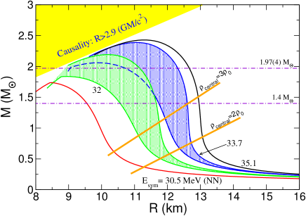
While real neutron stars are very complicated objects, their main global properties can usually be well-approximated by considering simple idealized models consisting of a perfect fluid in hydrostatic equilibrium. If rotation can be neglected to a first approximation (as is the case for the spin rates of most currently-known pulsars) then the model can be taken to be spherical and its structure obtained by solving the Tolman-Oppenheimer-Volkoff (TOV) equations Oppenheimer and Volkoff (1939), enabling one to calculate, for example, the stellar mass as a function of radius or of central density. Using the energy density defined as
| (168) |
where is the mass of neutron, and the pressure at zero temperature is given by
| (169) |
as inputs, the neutron star model is evaluated by integrating the TOV equations:
| (170) |
| (171) |
Here is the gravitational mass enclosed within a radius , and is the gravitational constant. The solution of the TOV equations for a given central density gives the profiles of , and as functions of radius , and also the total radius and mass , with defined as the distance where the pressure drops to zero. A sequence of models can be generated by specifying a succession of values for the central density. In Fig. 34 the mass (measured in solar masses M⊙) as a function of the radius (measured in km) is showed, as obtained from AFDMC calculations using different prescriptions for the EoS presented in the previous sections.
It is interesting to make a comparison between these results so as to see the changes caused by introduction of the various different features in the Hamiltonian. An objective of this type of work is to attempt to constrain microphysical models for neutron-star matter by making comparison with astronomical observations. This has become possible in the last few years, as discussed for example in Steiner et al. (2010), Ozel et al. (2010), Steiner and Gandolfi (2012) and Steiner et al. (2015). Further progress is anticipated within the next few years if gravitational waves from neutron star mergers can be detected. The most recently observed maximum neutron star masses are 1.97(2) M⊙ Demorest et al. (2010) and 2.01(4) M⊙ Antoniadis et al. (2013). These observations put the most severe constraints on the EoS, although the precise hadronic composition is still undetermined.
VI.2 Inhomogeneous Neutron Matter
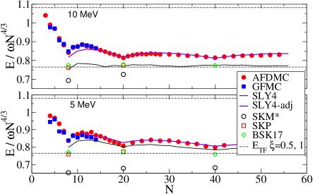
While the mass and radius of a neutron star depend primarily on the equation of state of neutron matter, the inner crust of the star contains inhomogeneous neutron matter immersed between very neutron-rich nuclei Ravenhall et al. (1983); Shternin et al. (2007); Brown and Cumming (2009). Similarly, the exterior of very neutron-rich nuclei is believed to have a significant excess of neutrons. This neutron distribution can be probed, for example, in parity-violating electron scattering.
Mean-field models including Skyrme and related models are typically fit to bulk properties of known nuclei, which are much nearer to isospin symmetry. They have sometimes also included results from ab-initio calculations of neutron matter directly in their fits, e.g., Chabanat et al. (1997, 1998). Historically, this is the only information used to constrain density functionals in the pure neutron matter limit.
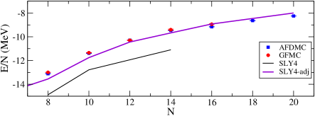
Therefore it is useful to perform ab-initio studies of inhomogeneous neutron matter at low and moderate densities. A study of neutron drops can provide constraints on density-functional studies of neutron-rich inhomogeneous matter, as well as the properties of neutron-rich nuclei that can be measured in terrestrial experiments. Gandolfi et al. (2011); Maris et al. (2013). It is also possible to study neutron-rich nuclei with an inert core of neutrons and protons, including realistic NN and 3N interactions between the neutrons. This approach has been used to study the binding energies of oxygen Gandolfi et al. (2006); Chang et al. (2004) and calcium isotopes Gandolfi et al. (2008b).
Calculations of neutron drops provide information about a variety of quantities that enter in the energy-density functional. Clearly the gradient term in pure neutron matter is important in neutron drops, this term has a large uncertainty in fits of known nuclei. The gradient term is important even in closed-shell arrangements of neutrons in an external well. Studying drops between the closed shell limits provides a variety of additional information. One can study the superfluid pairing of pure neutron drops, a very different environment from nuclei. The pairing is expected to play a more important role in dilute neutron matter, and may affect the shell closure. Similarly one can look at the purely isovector spin-orbit splitting by varying the number of neutrons around closed shells and possible sub-shell closures.
Early QMC calculations of very small neutron drops ( = 6,7,8) already indicated a substantial difference from traditional Skyrme models, which overbind the drops and yield a too-large spin-orbit splitting Pudliner et al. (1996); Smerzi et al. (1997); Pederiva et al. (2004). However these calculations did not systematically cover a wide range of neutron numbers and confinement potentials.
Both GFMC and AFDMC have been used to provide ab-initio results for neutron drops. The AV8′+UIX Hamiltonian, which produces an EoS consistent with known neutron star masses (see the previous section), has been used to constrain several modern Skyrme models Gandolfi et al. (2011); Maris et al. (2013). Several forms of the external well were considered, including harmonic oscillators (HO) of various frequency, as well as Wood-Saxon wells. The former produce a wider range of densities, particularly higher densities near the center of the trap, while in the latter the density saturates as in nuclei.
The results of these calculations are shown in Figs. 35 and 36. For the harmonic traps the energy is divided by the frequency of the trap times N4/3; this would be a constant for a free Fermi Gas in the Thomas-Fermi or local density approximation. The QMC results are shown as solid points. For a given Hamiltonian, the agreement between GFMC and AFDMC is very satisfactory. Results agree very well for the 10 MeV HO interaction, while for MeV, the AFDMC results are slightly higher than the GFMC ones; the maximum difference is , and more typically results are within . The bigger difference for the low-density drops produced by the 5-MeV well presumably arises because the importance function used in AFDMC does not include pairing, in contrast to the more complete treatment used in GFMC.
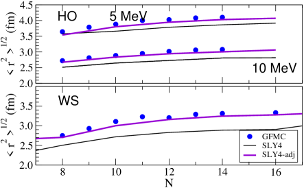
In both cases conventional Skyrme models overbind the drops. Since some of the Skyrme functionals have been fitted to the neutron matter EoS, the overbinding might be explained by the contributions given by the gradient term. As is evident from Fig. 35, closed shells are still found at = 8, 20, and 40 neutrons in the HO wells. These closed-shell states are almost exclusively sensitive to the neutron matter EoS and the isovector gradient terms, while the contributions from pairing and spin-orbit terms are very small. Instead, by examining drops with neutron numbers that differ slightly from closed shells, one can constrain the spin-orbit interaction. It has been found that a smaller isovector coupling, approximately 1/6 of the isoscalar coupling, reproduces rather accurately the ab-initio calculations for these drops. Results for half-filled-shell drops (e.g. = 14 or 30) and odd-even staggerings are sensitive to the pairing interactions as well as the spin-orbit force. Fixing the spin-orbit strength from near closed-shell drops, the pairing strength can be adjusted to fit the calculated spectra.
Adjusting these three parameters in the density functional to better describe energies for selected number of neutrons in the HO as described in Gandolfi et al. (2011) improves the agreement for all external fields and particle numbers considered. This is shown by the upper solid curves (SLY4-adj) in Fig. 35 and in Fig. 36.
The rms radii and density distributions of neutron drops are also useful checks of the density functionals. GFMC accurately computes these quantities. In Fig. 37 the radii computed using GFMC for different drops are compared to those computed using the original SLY4 Skyrme and the adjusted SLY4-adj for the two HO wells considered. Comparisons of the densities for = 8 and 14 in the HO wells are shown in Fig. 38. These two systems provide benchmarks of a closed-shell drop and of a half-filled-shell respectively. The adjusted-SLY4 gives much better evaluations of these observables than those obtained using the original SLY4 functional.
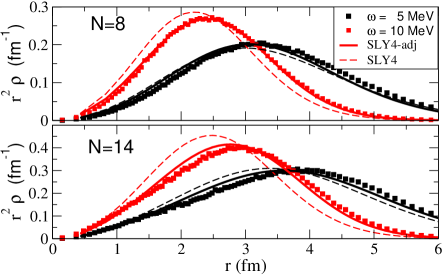
The QMC calculations can also be compared to predictions given by other methods. For example, in Fig. 39 the AFDMC results obtained using different Hamiltonians (indicated in the legend) are compared to the no core full configuration results obtained using the JISP16 interaction in no-core full configuration (NCFC) calculations Maris et al. (2013).
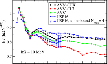
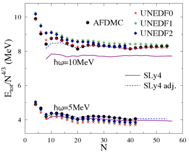
VII Conclusions and Future Directions
Quantum Monte Carlo methods have proved to be extremely valuable for studying the structure and reactions of nuclei and nucleonic matter with realistic nuclear interactions and currents. As illustrated in this review, QMC methods can simultaneously treat diverse phenomena across a range of momentum scales including strong tensor correlations at short distances and the associated electroweak responses, spectra and clustering and low-energy EM transitions in light nuclei, and superfluidity and the dense neutron matter equation of state. Across this range from the lightest nuclei to neutron matter the same nuclear models of interactions and currents are applicable. These models have been directly obtained from nucleon-nucleon scattering data and properties of the very lightest nuclei.
QMC methods and accurate interaction and current models provide quantitative predictions for spectra, electromagnetic moments, transition rates, form factors, asymptotic normalization constants, and other low-momentum properties of nuclei up to =12. The recent results on electromagnetic transitions in light nuclei is particularly encouraging, demonstrating conclusively the importance of realistic models of two-nucleon currents even at very low momentum transfer. The wide range of energies (up to 350 MeV lab) covered by these interactions also allow one to study the electroweak response at rather large momentum transfers, and to study the neutron matter equation of state up to the regime where the Fermi momentum is fm-1, a regime that controls the radius and much of the structure of neutron stars. Realistic models of the nuclear interaction predicted a stiff equation of state at high densities from the two- and three-nucleon repulsion. The recent observation of two-solar mass neutron stars confirms this behavior.
Progress has been due to a concerted effort of physicists studying nuclear interactions and currents, novel quantum Monte Carlo methods, and computer scientists and applied mathematicians enabling efficient computations on the largest available computers Bogner et al. (2013). The dramatic advances in computer architecture, and the fairly wide availability of these machines, have also been key.
Many important challenges will be addressed in the near future, in both light and heavy nuclei and nucleonic matter. In light nuclei the study of more complicated nuclear reactions will be important. These can address problems where it is difficult to conduct experiments, including reactions at very low energies where the Coulomb barrier suppresses the reaction rate, or reactions on unstable nuclei. In addition tests of fundamental symmetries, including electric dipole moments in light nuclei, can be addressed. Many of these problems require only moderate advances in theory and computation and it should be possible to address a significant number in the next few years.
Neutrino scattering and nuclear response is of fundamental interest in both fairly light nuclei like carbon and oxygen, and also in heavier nuclei like argon. Calculations of the charged-current carbon response will be very illuminating, in particular regarding the difference of neutrino to anti-neutrino cross sections. This plays a key role in future attempts to measure the neutrino mass hierarchy and the CP-violating phase using accelerator neutrinos. Calculations in heavier nuclei will allow us to explore the nuclear dependence of the quasielastic scattering, which is expected to be fairly small as in electron scattering.
The properties of heavy neutron-rich nuclei are also very important, particularly in light of the upcoming FRIB facility. The extreme neutron-rich nuclei play an important role in the r-process, and it will be very interesting to explore questions including pairing in neutron-rich nuclei and their weak response starting from fundamental interactions. Of course larger nuclei also provide important tests of fundamental symmetries, including electric dipole moments and neutrinoless double beta decay. It will be an important challenge to use quantum Monte Carlo techniques to study these problems.
The reliability and dynamic range of these models are extremely important in extrapolating to new regimes, particularly the neutron-rich matter found in supernovae and neutron stars. Questions to be addressed there include the equation of state and weak response of beta-stable matter, relevant to the cooling of neutron stars, and the response in hot low-density regimes characteristic of the surface where the neutrinos decouple in the core-collapse supernovae. Studies of the equation of state and its relevance to neutron star mergers are also important. Gravitational wave observations should be able to give much more precise information on the mass-radius relation in neutron stars.
We look forward to dramatic advances in theory and computation, including a more refined understanding of nuclear interactions and currents. Combined with exciting prospects in experiments and observation, we believe there is a bright future for nuclear physics and its connections to quantum few- and many-body theory, astrophysics, neutrino physics, and physics beyond the Standard Model.
Acknowledgements.
We are particularly indebted with A. Lovato for the careful reading of the manuscript and for the various critical comments. We also would like to thank A. Bulgac, A. Gezerlis, D. Lonardoni, A. Lovato, J. Lynn, K. M. Nollett, S. Pastore, S. Reddy, and A. Roggero for the useful discussions, and/or for sharing results. The work of J.C., S.G., S.C.P., and R.B.W. has been supported by the NUCLEI and previous UNEDF SciDAC projects. This research is also supported by the U.S. Department of Energy, Office of Nuclear Physics, under contracts DE-AC02-05CH11231 (S.G. and J.C.), DE-AC02-06CH11357 (S.C.P. and R.B.W.), and DE-AC05-06OR23177 (R.S.), by LISC, the Interdisciplinary Laboratory for Computational Science, a joint venture of the University of Trento and the Bruno Kessler Foundation (F.P.), and by National Science foundation grant PHY-1404405 (K.S.). Under an award of computer time provided by the INCITE program, this research used resources of the Argonne Leadership Computing Facility at Argonne National Laboratory, which is supported by the Office of Science of the U.S. Department of Energy under contract DE-AC02-06CH11357. This research also used resources provided by Los Alamos Open Supercomputing, by the National Energy Research Scientific Computing Center (NERSC), and by Argonne’s Laboratory Computing Resource Center.References
- Abe et al. (2012) Abe, T., P. Maris, T. Otsuka, N. Shimizu, Y. Utsuno, and J. P. Vary (2012), Phys. Rev. C 86, 054301.
- Abe and Seki (2009) Abe, T., and R. Seki (2009), Phys. Rev. C79, 054003.
- Acha et al. (2007) Acha, A., et al. (HAPPEX Collaboration) (2007), Phys. Rev. Lett. 98, 032301.
- Ackerbauer et al. (1998) Ackerbauer, P., et al. (1998), Phys. Lett. B 417, 224 .
- Adelberger et al. (2011) Adelberger, E. G., et al. (2011), Rev. Mod. Phys. 83, 195.
- Aguilar-Areval (2008) Aguilar-Areval, A. A. et al.. (MiniBooNE Collaboration) (2008), Phys. Rev. Lett. 100, 032301.
- Ahmed et al. (2012) Ahmed, Z., et al. (HAPPEX Collaboration) (2012), Phys. Rev. Lett. 108, 102001.
- Ahrens et al. (1987) Ahrens, L. A., et al. (1987), Phys. Rev. D 35, 785.
- Akmal et al. (1998) Akmal, A., V. R. Pandharipande, and D. G. Ravenhall (1998), Phys. Rev. C 58 (3), 1804.
- Amaldi et al. (1979) Amaldi, E., S. Fubini, and G. Furlan (1979), Springer Tracts in Modern Physics 93, 10.1007/BFb0048208.
- Amroun et al. (1994) Amroun, A., V. Breton, J.-M. Cavedon, B. Frois, D. Goutte, F. Juster, P. Leconte, J. Martino, Y. Mizuno, X.-H. Phan, S. Platchkov, I. Sick, and S. Williamson (1994), Nucl. Phys. A 579, 596.
- Anderson (1976) Anderson, J. B. (1976), J. Chem. Phys. 65 (10), 4121.
- Andreev et al. (2007) Andreev, V. A., et al. (MuCap Collaboration) (2007), Phys. Rev. Lett. 99, 032002.
- Aniol et al. (2004) Aniol, K. A., et al. (HAPPEX Collaboration) (2004), Phys. Rev. C 69, 065501.
- Antoniadis et al. (2013) Antoniadis, J., et al. (2013), Science 340 (6131).
- Bacca and Pastore (2014) Bacca, S., and S. Pastore (2014), J. Phys. G; Nucl. Part. Phys. 41, 123002.
- Baker et al. (1981) Baker, N. J., A. M. Cnops, P. L. Connolly, S. A. Kahn, H. G. Kirk, M. J. Murtagh, R. B. Palmer, N. P. Samios, and M. Tanaka (1981), Phys. Rev. D 23, 2499.
- Barletta et al. (2009) Barletta, P., C. Romero-Redondo, A. Kievsky, M. Viviani, and E. Garrido (2009), Phys. Rev. Lett. 103, 090402.
- Barrett et al. (2013) Barrett, B. R., P. Navr til, and J. P. Vary (2013), Progress in Particle and Nuclear Physics 69 (0), 131 .
- Beane et al. (2013) Beane, S. R., E. Chang, S. D. Cohen, W. Detmold, H. W. Lin, T. C. Luu, K. Orginos, A. Parreño, M. J. Savage, and A. Walker-Loud (2013), Phys. Rev. D 87, 034506.
- Bedaque and van Kolck (2002) Bedaque, P., and U. van Kolck (2002), Ann. Rev. Nucl. Part. Sci. 52, 339.
- Beise et al. (2005) Beise, E., M. Pitt, and D. Spayde (2005), Progress in Particle and Nuclear Physics 54 (1), 289 .
- Benhar et al. (2010) Benhar, O., P. Coletti, and D. Meloni (2010), Phys. Rev. Lett. 105, 132301.
- Bernard et al. (2011) Bernard, V., E. Epelbaum, H. Krebs, and U.-G. Meissner (2011), Phys. Rev. C 84, 054001.
- Bernard et al. (1994) Bernard, V., N. Kaiser, and U.-G. Meissner (1994), Phys. Rev. D 50, 6899.
- B.J. Hammond (1994) B.J. Hammond, P. R., W.A. Lester (1994), Monte Carlo Methods in ab Initio Quantum Chemistry (World Scientific, Singapore).
- Bogner et al. (2013) Bogner, S., A. Bulgac, J. A. Carlson, J. Engel, G. Fann, et al. (2013), Comput. Phys. Commun. 184, 2235.
- Bogner et al. (2010) Bogner, S., R. Furnstahl, and A. Schwenk (2010), Progress in Particle and Nuclear Physics 65 (1), 94.
- Bonett-Matiz et al. (2013) Bonett-Matiz, M., A. Mukherjee, and Y. Alhassid (2013), Phys. Rev. C 88, 011302.
- Bonnard and Juillet (2013) Bonnard, J., and O. Juillet (2013), Phys. Rev. Lett. 111, 012502.
- Brida et al. (2011) Brida, I., S. C. Pieper, and R. B. Wiringa (2011), Phys. Rev. C 84, 024319.
- Brown and Cumming (2009) Brown, E. F., and A. Cumming (2009), Astrophys. J. 698, 1020.
- Bryan (1990) Bryan, R. (1990), European Biophysics Journal 18 (3), 165.
- Butkevich (2010) Butkevich, A. V. (2010), Phys. Rev. C 82, 055501.
- Carlson (1986) Carlson, C. E. (1986), Phys. Rev. D 34, 2704.
- Carlson (1987) Carlson, J. (1987), Phys. Rev. C 36 (5), 2026.
- Carlson (1988) Carlson, J. (1988), Phys. Rev. C 38 (4), 1879.
- Carlson (2003) Carlson, J. (2003), Eur. Phys. J. A 17, 463.
- Carlson et al. (2003a) Carlson, J., S.-Y. Chang, V. R. Pandharipande, and K. E. Schmidt (2003a), Phys. Rev. Lett. 91 (5), 050401.
- Carlson et al. (2012) Carlson, J., S. Gandolfi, and A. Gezerlis (2012), PTEP 2012, 01A209.
- Carlson et al. (2002) Carlson, J., J. Jourdan, R. Schiavilla, and I. Sick (2002), Phys. Rev. C 65, 024002.
- Carlson et al. (2003b) Carlson, J., J. Morales, V. R. Pandharipande, and D. G. Ravenhall (2003b), Phys. Rev. C 68 (2), 025802.
- Carlson et al. (1993) Carlson, J., V. R. Pandharipande, and R. Schiavilla (1993), Phys. Rev. C 47 (2), 484.
- Carlson et al. (1983) Carlson, J., V. R. Pandharipande, and R. B. Wiringa (1983), Nucl. Phys. A 401, 59.
- Carlson et al. (1991) Carlson, J., D. O. Riska, R. Schiavilla, and R. B. Wiringa (1991), Phys. Rev. C 44, 619.
- Carlson and Schiavilla (1992) Carlson, J., and R. Schiavilla (1992), Phys. Rev. Lett. 68, 3682.
- Carlson and Schiavilla (1994) Carlson, J., and R. Schiavilla (1994), Phys. Rev. C 49, R2880.
- Carlson and Schiavilla (1998) Carlson, J., and R. Schiavilla (1998), Rev. Mod. Phys. 70 (3), 743.
- Carlson et al. (1987) Carlson, J., K. E. Schmidt, and M. H. Kalos (1987), Phys. Rev. C 36, 27.
- Ceperley et al. (1977) Ceperley, D., G. V. Chester, and M. H. Kalos (1977), Phys. Rev. B 16 (7), 3081.
- Ceperley (1995) Ceperley, D. M. (1995), Rev. Mod. Phys. 67, 279.
- Chabanat et al. (1997) Chabanat, E., P. Bonche, P. Haensel, J. Meyer, and R. Schaeffer (1997), Nucl. Phys. A 627, 710.
- Chabanat et al. (1998) Chabanat, E., P. Bonche, P. Haensel, J. Meyer, and R. Schaeffer (1998), Nucl. Phys. A 635, 231.
- Chang et al. (2004) Chang, S. Y., J. Morales, Jr., V. R. Pandharipande, D. G. Ravenhall, J. Carlson, S. C. Pieper, R. B. Wiringa, and K. E. Schmidt (2004), Nucl. Phys. A 746, 215.
- Chemtob and Rho (1971) Chemtob, M., and M. Rho (1971), Nucl. Phys. A 163, 1.
- Chen et al. (2010) Chen, L.-W., C. M. Ko, B.-A. Li, and J. Xu (2010), Phys. Rev. C 82 (2), 024321.
- Chernykh et al. (2010) Chernykh, M., H. Feldmeier, T. Neff, P. von Neumann-Cosel, and A. Richter (2010), Phys. Rev. Lett. 105, 022501.
- Coelho et al. (1983) Coelho, H. T., T. K. Das, and M. R. Robilotta (1983), Phys. Rev. C 28, 1812.
- Cohen and Kurath (1967) Cohen, S., and D. Kurath (1967), Nucl. Phys. A 101, 1.
- Coon et al. (1979) Coon, S. A., M. D. Scadron, P. C. McNamee, B. R. Barrett, D. W. E. Blatt, and B. H. J. McKellar (1979), Nucl. Phys. A 317, 242.
- Czarnecki et al. (2007) Czarnecki, A., W. J. Marciano, and A. Sirlin (2007), Phys. Rev. Lett. 99, 032003.
- Danielewicz et al. (2002) Danielewicz, P., R. Lacey, and W. G. Lynch (2002), Science 298, 1592.
- De Vries et al. (1987) De Vries, H., C. W. De Jager, and C. De Vries (1987), Atomic Data and Nuclear Data Tables 36, 495.
- Demorest et al. (2010) Demorest, P., T. Pennucci, S. Ransom, M. Roberts, and J. Hessels (2010), Nature 467, 1081.
- Dickhoff and Barbieri (2004) Dickhoff, W., and C. Barbieri (2004), Progress in Particle and Nuclear Physics 52 (2), 377 .
- Donnelly and Sick (1984) Donnelly, T. W., and I. Sick (1984), Rev. Mod. Phys. 56, 461.
- Edmonds (1957) Edmonds, A. (1957), Princeton University Press 16, 1.
- Entem and Machleidt (2002) Entem, D., and R. Machleidt (2002), Phys. Lett. B 524, 93.
- Entem and Machleidt (2003) Entem, D., and R. Machleidt (2003), Phys. Rev. C 68, 041001.
- Epelbaum et al. (1998) Epelbaum, E., W. Gloeckle, and U.-G. Meissner (1998), Nuc. Phys. A 637, 107.
- Epelbaum et al. (2009) Epelbaum, E., H.-W. Hammer, and U.-G. Meißner (2009), Rev. Mod. Phys. 81 (4), 1773.
- Epelbaum et al. (2012) Epelbaum, E., H. Krebs, T. A. Lahde, D. Lee, and U.-G. Meissner (2012), Phys. Rev. Lett. 109, 252501.
- Epelbaum et al. (2014) Epelbaum, E., H. Krebs, T. A. Lähde, D. Lee, U.-G. Meißner, and G. Rupak (2014), Phys. Rev. Lett. 112, 102501.
- Epelbaum et al. (2011) Epelbaum, E., H. Krebs, D. Lee, and U.-G. Meissner (2011), Phys. Rev. Lett. 106, 192501.
- Epelbaum and Meissner (1999) Epelbaum, E., and U.-G. Meissner (1999), Phys. Lett. B 461, 287.
- Epelbaum et al. (2002) Epelbaum, E., A. Nogga, W. Gloeckle, H. Kamada, U. G. Meissner, et al. (2002), Phys. Rev. C 66, 064001.
- Esbensen (2004) Esbensen, H. (2004), Phys. Rev. C 70, 047603.
- Fantoni and Schmidt (2001) Fantoni, S., and K. E. Schmidt (2001), Nucl. Phys. A 690, 456.
- Feenberg and Wigner (1937) Feenberg, E., and E. Wigner (1937), Phys. Rev. 51, 95.
- Foulkes et al. (2001) Foulkes, W. M. C., L. Mitas, R. J. Needs, and G. Rajagopal (2001), Rev. Mod. Phys. 73, 33.
- Friar (1977) Friar, J. (1977), Ann. Phys. (N.Y.) 104, 380.
- Friar et al. (1999) Friar, J. L., D. Hüber, and U. van Kolck (1999), Phys. Rev. C 59, 53.
- Friar and van Kolck (1999) Friar, J. L., and U. van Kolck (1999), Phys. Rev. C 60, 034006.
- Friar et al. (2004) Friar, J. L., U. van Kolck, M. C. M. Rentmeester, and R. G. E. Timmermans (2004), Phys. Rev. C 70, 044001.
- Friar et al. (2005) Friar, J. L., G. L. Payne, and U. van Kolck (2005), Phys. Rev. C 71, 024003.
- Fujita and Miyazawa (1957) Fujita, J., and H. Miyazawa (1957), Prog. Theor. Phys. 17, 360.
- Gandolfi (2007) Gandolfi, S. (2007), arXiv:0712.1364 [nucl-th] Ph.D. thesis, University of Trento, Italy.
- Gandolfi et al. (2011) Gandolfi, S., J. Carlson, and S. C. Pieper (2011), Phys. Rev. Lett. 106 (1), 012501.
- Gandolfi et al. (2012) Gandolfi, S., J. Carlson, and S. Reddy (2012), Phys. Rev. C 85 (3), 032801.
- Gandolfi et al. (2014) Gandolfi, S., J. Carlson, S. Reddy, A. W. Steiner, and R. B. Wiringa (2014), Eur. Phys. J. A 50, 10.
- Gandolfi et al. (2008a) Gandolfi, S., A. Y. Illarionov, S. Fantoni, F. Pederiva, and K. E. Schmidt (2008a), Phys. Rev. Lett. 101, 132501.
- Gandolfi et al. (2009a) Gandolfi, S., A. Y. Illarionov, F. Pederiva, K. E. Schmidt, and S. Fantoni (2009a), Phys. Rev. C 80, 045802.
- Gandolfi et al. (2009b) Gandolfi, S., A. Y. Illarionov, K. E. Schmidt, F. Pederiva, and S. Fantoni (2009b), Phys. Rev. C 79, 054005.
- Gandolfi et al. (2014) Gandolfi, S., A. Lovato, J. Carlson, and K. E. Schmidt (2014), Phys. Rev. C 90, 061306.
- Gandolfi et al. (2008b) Gandolfi, S., F. Pederiva, and S. a Beccara (2008b), Eur. Phys. J. A 35, 207.
- Gandolfi et al. (2006) Gandolfi, S., F. Pederiva, S. Fantoni, and K. E. Schmidt (2006), Phys. Rev. C 73, 044304.
- Gezerlis and Carlson (2008) Gezerlis, A., and J. Carlson (2008), Phys. Rev. C 77, 032801(R).
- Gezerlis and Carlson (2010) Gezerlis, A., and J. Carlson (2010), Phys. Rev. C 81, 025803.
- Gezerlis et al. (2014) Gezerlis, A., I. Tews, E. Epelbaum, M. Freunek, S. Gandolfi, K. Hebeler, A. Nogga, and A. Schwenk (2014), Phys. Rev. C 90, 054323.
- Gezerlis et al. (2013) Gezerlis, A., I. Tews, E. Epelbaum, S. Gandolfi, K. Hebeler, et al. (2013), Phys. Rev. Lett. 111 (3), 032501.
- Giorgini et al. (2008) Giorgini, S., L. P. Pitaevskii, and S. Stringari (2008), Rev. Mod. Phys. 80, 1215.
- Girlanda (2008) Girlanda, L. (2008), Phys. Rev. C 77, 067001.
- Girlanda et al. (2010) Girlanda, L., A. Kievsky, L. Marcucci, S. Pastore, R. Schiavilla, et al. (2010), Phys. Rev. Lett. 105, 232502.
- Girlanda et al. (2011) Girlanda, L., A. Kievsky, and M. Viviani (2011), Phys. Rev. C 84, 014001.
- Gorringe and Fearing (2003) Gorringe, T., and H. W. Fearing (2003), Rev. Mod. Phys. 76, 31.
- Grinyer et al. (2011) Grinyer, G. F., et al. (2011), Phys. Rev. Lett. 106, 162502.
- Grinyer et al. (2012) Grinyer, G. F., et al. (2012), Phys. Rev. C 86, 024315.
- Hadjimichael et al. (1983) Hadjimichael, E., B. Goulard, and R. Bornais (1983), Phys. Rev. C 27, 831.
- Hagen et al. (2014) Hagen, G., T. Papenbrock, A. Ekström, K. A. Wendt, G. Baardsen, S. Gandolfi, M. Hjorth-Jensen, and C. J. Horowitz (2014), Phys. Rev. C 89, 014319.
- Hagen et al. (2014) Hagen, G., T. Papenbrock, M. Hjorth-Jensen, and D. J. Dean (2014), Reports on Progress in Physics 77 (9), 096302.
- Haxton and Holstein (2013) Haxton, W. C., and B. R. Holstein (2013), Prog. Part. Nucl. Phys. 71, 185.
- Henley et al. (1979) Henley, E. M., G. A. Miller, M. Rho, and D. Wilkinson (1979), Mesons in Nuclei, Vol. 1, (North-Holland, Amsterdam) , 405.
- Hyde-Wright and de Jager (2004) Hyde-Wright, C. E., and K. de Jager (2004), Annual Review of Nuclear and Particle Science 54 (1), 217.
- Ishii et al. (2007) Ishii, N., S. Aoki, and T. Hatsuda (2007), Phys. Rev. Lett. 99, 022001.
- Jarrell and Gubernatis (1996) Jarrell, M., and J. E. Gubernatis (1996), Physics Reports 269 (3), 133.
- Jourdan (1996) Jourdan, J. (1996), Nucl. Phys. A 603, 117.
- Kalos (1962) Kalos, M. H. (1962), Phys. Rev. 128, 1791.
- Kamada et al. (2001) Kamada, H., A. Nogga, W. Glöckle, E. Hiyama, M. Kamimura, K. Varga, Y. Suzuki, M. Viviani, A. Kievsky, S. Rosati, J. Carlson, S. C. Pieper, R. B. Wiringa, P. Navrátil, B. R. Barrett, N. Barnea, W. Leidemann, and G. Orlandini (2001), Phys. Rev. C 64 (4), 044001.
- Kammel and Kubodera (2010) Kammel, P., and K. Kubodera (2010), Annual Review of Nuclear and Particle Science 60 (1), 327.
- Kay et al. (2013) Kay, B. P., J. P. Schiffer, and S. J. Freeman (2013), Phys. Rev. Lett. 111, 042502.
- Kitagaki et al. (1983) Kitagaki, T., et al. (1983), Phys. Rev. D 28, 436.
- van Kolck (1994) van Kolck, U. (1994), Phys. Rev. C 49, 2932.
- Kölling et al. (2009) Kölling, S., E. Epelbaum, H. Krebs, and U.-G. Meissner (2009), Phys. Rev. C 80, 045502.
- Kölling et al. (2011) Kölling, S., E. Epelbaum, H. Krebs, and U.-G. Meissner (2011), Phys. Rev. C 84, 054008.
- Koonin et al. (1997) Koonin, S. E., D. J. Dean, and K. Langanke (1997), Phys. Rep. 278, 1.
- Korover et al. (2014) Korover, I., et al. ((Jefferson Lab Hall A Collaboration)) (2014), Phys. Rev. Lett. 113, 022501.
- Kortelainen et al. (2014) Kortelainen, M., J. McDonnell, W. Nazarewicz, E. Olsen, P.-G. Reinhard, J. Sarich, N. Schunck, S. M. Wild, D. Davesne, J. Erler, and A. Pastore (2014), Phys. Rev. C 89, 054314.
- Kubodera et al. (1978) Kubodera, K., J. Delorme, and M. Rho (1978), Phys. Rev. Lett. 40, 755.
- Kumar (1974) Kumar, N. (1974), Nuclear Physics A 225 (2), 221 .
- Kurath (1979) Kurath, D. (1979), Nuclear Physics A 317 (1), 175 .
- Kurylov et al. (2002) Kurylov, A., M. J. Ramsey-Musolf, and P. Vogel (2002), Phys. Rev. C 65, 055501.
- Lapikás et al. (1999) Lapikás, L., J. Wesseling, and R. B. Wiringa (1999), Phys. Rev. Lett. 82, 4404.
- Lattimer and Lim (2013) Lattimer, J. M., and Y. Lim (2013), Astrophys. J. 771, 51.
- Lattimer and Prakash (2001) Lattimer, J. M., and M. Prakash (2001), Astrophys. J. 550, 426.
- LBNE Collaboration et al. (2013) LBNE Collaboration,, C. Adams, D. Adams, T. Akiri, T. Alion, K. Anderson, C. Andreopoulos, M. Andrews, I. Anghel, J. C. Costa dos Anjos, and et al. (2013), ArXiv e-prints arXiv:1307.7335 [hep-ex] .
- Lee (2009) Lee, D. (2009), Prog. in Part. and Nucl. Phys. 63, 117.
- Lee et al. (2004) Lee, D., B. Borasoy, and T. Schaefer (2004), Phys. Rev. C 70, 014007.
- Lee and Schäfer (2006) Lee, D., and T. Schäfer (2006), Phys. Rev. C73, 015201.
- Leidemann and Orlandini (2013) Leidemann, W., and G. Orlandini (2013), Prog. Part. Nucl. Phys. 68, 158.
- Lin et al. (2001) Lin, C., F. H. Zong, and D. M. Ceperley (2001), Phys. Rev. E 64 (1), 016702.
- Lin and Liou (1991) Lin, D., and M. K. Liou (1991), Phys. Rev. C 43, R930.
- Liu et al. (1974) Liu, K. S., M. H. Kalos, and G. V. Chester (1974), Phys. Rev. A 10, 303.
- Lomnitz-Adler et al. (1981) Lomnitz-Adler, J., V. Pandharipande, and R. Smith (1981), Nucl. Phys. A 361 (2), 399.
- Lonardoni et al. (2013) Lonardoni, D., S. Gandolfi, and F. Pederiva (2013), Phys. Rev. C 87, 041303.
- Lonardoni et al. (2015) Lonardoni, D., A. Lovato, S. Gandolfi, and F. Pederiva (2015), Phys. Rev. Lett. 114, 092301.
- Lonardoni et al. (2014) Lonardoni, D., F. Pederiva, and S. Gandolfi (2014), Phys. Rev. C 89, 014314.
- Lovato et al. (2013) Lovato, A., S. Gandolfi, R. Butler, J. Carlson, E. Lusk, S. C. Pieper, and R. Schiavilla (2013), Phys. Rev. Lett. 111, 092501.
- Lovato et al. (2014) Lovato, A., S. Gandolfi, J. Carlson, S. C. Pieper, and R. Schiavilla (2014), Phys. Rev. Lett. 112, 182502.
- Lovato et al. (2015) Lovato, A., S. Gandolfi, J. Carlson, S. C. Pieper, and R. Schiavilla (2015), arxiv.org/abs/1501.01981 .
- Lu et al. (2013) Lu, Z.-T., P. Mueller, G. W. F. Drake, W. Nörtershäuser, S. C. Pieper, and Z.-C. Yan (2013), Rev. Mod. Phys. 85, 1383.
- Lusk et al. (2010) Lusk, E., S. Pieper, and R. Butler (2010), SciDAC Review 17, 30.
- Lynn et al. (2014) Lynn, J., J. Carlson, E. Epelbaum, S. Gandolfi, A. Gezerlis, et al. (2014), Phys. Rev. Lett. 113 (19), 192501.
- Lynn and Schmidt (2012) Lynn, J. E., and K. E. Schmidt (2012), Phys. Rev. C 86 (1), 014324.
- Macfarlane and French (1960) Macfarlane, M. H., and J. B. French (1960), Rev. Mod. Phys. 32, 567.
- Machleidt (2001) Machleidt, R. (2001), Phys. Rev. C 63, 024001.
- Machleidt and Entem (2011) Machleidt, R., and D. Entem (2011), Phys. Rep. 503, 1.
- Machleidt et al. (1996) Machleidt, R., F. Sammarruca, and Y. Song (1996), Phys. Rev. C 53 (4), R1483.
- Marcucci et al. (2012) Marcucci, L. E., A. Kievsky, S. Rosati, R. Schiavilla, and M. Viviani (2012), Phys. Rev. Lett. 108, 052502.
- Marcucci et al. (2008) Marcucci, L. E., M. Pervin, S. C. Pieper, R. Schiavilla, and R. B. Wiringa (2008), Phys. Rev. C 78, 065501.
- Marcucci et al. (2011) Marcucci, L. E., M. Piarulli, M. Viviani, L. Girlanda, A. Kievsky, S. Rosati, and R. Schiavilla (2011), Phys. Rev. C 83, 014002.
- Marcucci et al. (2000) Marcucci, L. E., R. Schiavilla, M. Viviani, A. Kievsky, S. Rosati, and J. F. Beacom (2000), Phys. Rev. C 63, 015801.
- Marcucci et al. (2005) Marcucci, L. E., M. Viviani, R. Schiavilla, A. Kievsky, and S. Rosati (2005), Phys. Rev. C 72, 014001.
- Maris et al. (2013) Maris, P., J. P. Vary, S. Gandolfi, J. Carlson, and S. C. Pieper (2013), Phys. Rev. C 87, 054318.
- Mathiot (1989) Mathiot, J.-F. (1989), Physics Reports 173, 63 .
- McCutchan et al. (2012) McCutchan, E. A., C. J. Lister, S. C. Pieper, R. B. Wiringa, D. Seweryniak, J. P. Greene, P. F. Bertone, M. P. Carpenter, C. J. Chiara, G. Gürdal, C. R. Hoffman, R. V. F. Janssens, T. L. Khoo, T. Lauritsen, and S. Zhu (2012), Phys. Rev. C 86, 014312.
- McVoy and Van Hove (1962) McVoy, K. W., and L. Van Hove (1962), Phys. Rev. 125, 1034.
- Metropolis et al. (1953) Metropolis, N., A. W. Rosenbluth, M. N. Rosenbluth, A. H. Teller, and E. Teller (1953), The Journal of Chemical Physics 21 (6), 1087.
- Miller et al. (1982) Miller, K. L., et al. (1982), Phys. Rev. D 26, 537.
- Moskowitz et al. (1982) Moskowitz, J. W., K. E. Schmidt, M. Lee, and M. H. Kalos (1982), J. Chem. Phys. 77, 349.
- Muller et al. (2000) Muller, H., S. Koonin, R. Seki, and U. van Kolck (2000), Phys. Rev. C61, 044320.
- Nakamura (2010) Nakamura, K. et al.. (2010), Journal of Physics G: Nuclear and Particle Physics 37 (7A), 075021.
- Navratil (2007) Navratil, P. (2007), Few-Body Syst. 41, 117.
- Navrátil et al. (2007) Navrátil, P., V. G. Gueorguiev, J. P. Vary, W. E. Ormand, and A. Nogga (2007), Phys. Rev. Lett. 99, 042501.
- Nelder and Mead (1965) Nelder, J. A., and R. Mead (1965), The Computer Journal 7 (4), 308.
- Nightingale and Umrigar (1999) Nightingale, M., and C. Umrigar (1999), Quantum Monte Carlo Methods in Physics and Chemistry (Springer).
- NNDC (2014) NNDC, (2014), “Nudat 2,” http://www.nndc.bnl.gov/nudat2/chartNuc.jsp.
- Nollett (2012) Nollett, K. M. (2012), Phys. Rev. C 86, 044330.
- Nollett et al. (2007) Nollett, K. M., S. C. Pieper, R. B. Wiringa, J. Carlson, and G. Hale (2007), Phys. Rev. Lett. 99, 022502.
- Nollett and Wiringa (2011) Nollett, K. M., and R. B. Wiringa (2011), Phys. Rev. C 83, 041001.
- Nörtershäuser and et al. (2009) Nörtershäuser, N., and et al. (2009), Phys. Rev. Lett. 102, 062503.
- Nörtershäuser et al. (2011) Nörtershäuser, N., T. Neff, R. Sánchez, and I. Sick (2011), Phys. Rev. C 84, 024307.
- Oppenheimer and Volkoff (1939) Oppenheimer, J. R., and G. M. Volkoff (1939), Phys. Rev. 55, 374.
- Ordonez et al. (1996) Ordonez, C., L. Ray, and U. van Kolck (1996), Phys. Rev. C 53, 2086.
- Otsuka et al. (2001) Otsuka, T., M. Honma, T. Mizusaki, N. Shimizu, and Y. Utsuno (2001), Progress in Particle and Nuclear Physics 47 (1), 319 .
- Ozel et al. (2010) Ozel, F., G. Baym, and T. Guver (2010), Phys. Rev. D82, 101301.
- Pandharipande et al. (1997) Pandharipande, V. R., I. Sick, and P. K. A. deWitt Huberts (1997), Rev. Mod. Phys. 69 (3), 961.
- Pandharipande and Wiringa (1979) Pandharipande, V. R., and R. B. Wiringa (1979), Rev. Mod. Phys. 51 (4), 821.
- Park et al. (1993) Park, T.-S., D.-P. Min, and M. Rho (1993), Phys. Rep. 233, 341.
- Park et al. (1996) Park, T.-S., D.-P. Min, and M. Rho (1996), Nucl. Phys. A 596, 515.
- Pastore (2014) Pastore, S. (2014), private communication .
- Pastore et al. (2011) Pastore, S., L. Girlanda, R. Schiavilla, and M. Viviani (2011), Phys. Rev. C 84, 024001.
- Pastore et al. (2009) Pastore, S., L. Girlanda, R. Schiavilla, M. Viviani, and R. Wiringa (2009), Phys. Rev. C 80, 034004.
- Pastore et al. (2013) Pastore, S., S. C. Pieper, R. Schiavilla, and R. B. Wiringa (2013), Phys. Rev. C 87, 035503.
- Pastore et al. (2014) Pastore, S., R. B. Wiringa, S. C. Pieper, and R. Schiavilla (2014), Phys. Rev. C 90, 024321.
- Pederiva et al. (2004) Pederiva, F., A. Sarsa, K. E. Schmidt, and S. Fantoni (2004), Nucl. Phys. A 742, 255.
- Pervin et al. (2007) Pervin, M., S. C. Pieper, and R. B. Wiringa (2007), Phys. Rev. C 76, 064319.
- Peshkin (1960) Peshkin, M. (1960), Phys. Rev. 121, 636.
- Piarulli et al. (2013) Piarulli, M., L. Girlanda, L. Marcucci, S. Pastore, R. Schiavilla, and M. Viviani (2013), Phys. Rev. C 87, 014006.
- Piarulli et al. (2015) Piarulli, M., L. Girlanda, R. Schiavilla, R. N. Pérez, J. E. Amaro, and E. R. Arriola (2015), Phys. Rev. C 91, 024003.
- Pieper (2008a) Pieper, S. C. (2008a), AIP Conf. Proc. 1011, 143.
- Pieper (2008b) Pieper, S. C. (2008b), in Proceedings of the ”Enrico Fermi” Summer School, Course CLXIX, Nuclear Structure far from Stability: New Physics and new Technology, edited by A. Covello, F. Iachello, R. A. Ricci, and G. Maino (IOS Press, Amsterdam) p. 111, reprinted in La Rivista del Nuovo Cimento, 31, 709, (2008).
- Pieper (2015) Pieper, S. C. (2015), unpublished .
- Pieper and Carlson (2015) Pieper, S. C., and J. Carlson (2015), unpublished .
- Pieper et al. (2001) Pieper, S. C., V. R. Pandharipande, R. B. Wiringa, and J. Carlson (2001), Phys. Rev. C 64 (1), 014001.
- Pieper et al. (2002) Pieper, S. C., K. Varga, and R. B. Wiringa (2002), Phys. Rev. C 66 (4), 044310.
- Pieper et al. (2004) Pieper, S. C., R. B. Wiringa, and J. Carlson (2004), Phys. Rev. C 70, 054325.
- Pieper et al. (1992) Pieper, S. C., R. B. Wiringa, and V. R. Pandharipande (1992), Phys. Rev. C 46 (5), 1741.
- Pinkston and Satchler (1965) Pinkston, W. T., and G. R. Satchler (1965), Nucl. Phys. 72, 641.
- Preston (1962) Preston, M. A. (1962), Physics of the Nucleus, (Addison-Wesley, Reading, Massachusetts) , 299.
- Pudliner et al. (1997) Pudliner, B. S., V. R. Pandharipande, J. Carlson, S. C. Pieper, and R. B. Wiringa (1997), Phys. Rev. C 56 (4), 1720.
- Pudliner et al. (1995) Pudliner, B. S., V. R. Pandharipande, J. Carlson, and R. B. Wiringa (1995), Phys. Rev. Lett. 74 (22), 4396.
- Pudliner et al. (1996) Pudliner, B. S., A. Smerzi, J. Carlson, V. R. Pandharipande, S. C. Pieper, and D. G. Ravenhall (1996), Phys. Rev. Lett. 76 (14), 2416.
- Purcell et al. (2010) Purcell, J. E., J. H. Kelley, E. Kwan, C. G. Sheu, and H. R. Weller (2010), Nucl. Phys. A 848, 1.
- Ravenhall et al. (1983) Ravenhall, D. G., C. J. Pethick, and J. R. Wilson (1983), Phys. Rev. Lett. 50 (26), 2066.
- Riska and Brown (1972) Riska, D., and G. Brown (1972), Phys. Lett. B 38 (4), 193 .
- Riska (1985a) Riska, D. O. (1985a), Phys. Scr. 31, 107.
- Riska (1985b) Riska, D. O. (1985b), Phys. Scr. 31, 471.
- Riska (1989) Riska, D. O. (1989), Phys. Rep. 181, 207.
- Riska and Poppius (1985) Riska, D. O., and M. Poppius (1985), Phys. Scr. 32, 581.
- Roggero et al. (2014) Roggero, A., A. Mukherjee, and F. Pederiva (2014), Phys. Rev. Lett. 112, 221103.
- Sachs (1948) Sachs, R. G. (1948), Phys. Rev. 74, 433.
- Saito et al. (1990) Saito, T.-Y., Y. Wu, S. Ishikawa, and T. Sasakawa (1990), Phys. Lett. B 242 (1), 12 .
- Sarsa et al. (2003) Sarsa, A., S. Fantoni, K. E. Schmidt, and F. Pederiva (2003), Phys. Rev. C 68 (2), 024308.
- Schiavilla and Pandharipande (2002) Schiavilla, R., and V. R. Pandharipande (2002), Phys. Rev. C 65, 064009.
- Schiavilla et al. (1989) Schiavilla, R., V. R. Pandharipande, and D. O. Riska (1989), Phys. Rev. C 40, 2294.
- Schiavilla et al. (1990) Schiavilla, R., V. R. Pandharipande, and D. O. Riska (1990), Phys. Rev. C 41, 309.
- Schiavilla et al. (1986) Schiavilla, R., V. R. Pandharipande, and R. B. Wiringa (1986), Nucl. Phys. A449, 219.
- Schiavilla et al. (1998) Schiavilla, R., V. G. J. Stoks, W. Glöckle, H. Kamada, A. Nogga, J. Carlson, R. Machleidt, V. R. Pandharipande, R. B. Wiringa, A. Kievsky, S. Rosati, and M. Viviani (1998), Phys. Rev. C 58, 1263.
- Schiavilla and Wiringa (2002) Schiavilla, R., and R. Wiringa (2002), Phys. Rev. C 65, 054302.
- Schiavilla et al. (1993) Schiavilla, R., R. B. Wiringa, and J. Carlson (1993), Phys. Rev. Lett. 70, 3856.
- Schiavilla et al. (1992) Schiavilla, R., R. B. Wiringa, V. R. Pandharipande, and J. Carlson (1992), Phys. Rev. C 45, 2628.
- Schiavilla et al. (2007) Schiavilla, R., R. B. Wiringa, S. C. Pieper, and J. Carlson (2007), Phys. Rev. Lett. 98, 132501.
- Schmidt and Ceperley (1992) Schmidt, K., and D. Ceperley (1992), The Monte Carlo Method in Condensed Matter Physics (ed by K. Binder Springer, Berlin).
- Schmidt and Fantoni (1999) Schmidt, K. E., and S. Fantoni (1999), Phys. Lett. B 446, 99.
- Schmidt and Lee (1995) Schmidt, K. E., and M. A. Lee (1995), Phys. Rev. E 51, 5495.
- Seki and van Kolck (2006) Seki, R., and U. van Kolck (2006), Phys. Rev. C73, 044006.
- Shen et al. (2012) Shen, G., L. Marcucci, J. Carlson, S. Gandolfi, and R. Schiavilla (2012), Phys. Rev. C86, 035503.
- Shiner et al. (1994) Shiner, D., R. Dixson, and V. Vedantham (1994), Phys. Rev. Lett. 74, 3553.
- Shternin et al. (2007) Shternin, P. S., D. G. Yakovlev, P. Haensel, and A. Y. Potekhin (2007), Mon. Not. R. Astron. Soc. 382, L43.
- Sick (1982) Sick, I. (1982), Phys. Lett. B 116, 212.
- Sick (2013) Sick, I. (2013), Private communication.
- Smerzi et al. (1997) Smerzi, A., D. G. Ravenhall, and V. R. Pandharipande (1997), Phys. Rev. C 56 (5), 2549.
- Spayde et al. (2000) Spayde, D. T., et al. ((SAMPLE Collaboration)) (2000), Phys. Rev. Lett. 84, 1106.
- Steiner and Gandolfi (2012) Steiner, A. W., and S. Gandolfi (2012), Phys. Rev. Lett. 108, 081102.
- Steiner et al. (2015) Steiner, A. W., S. Gandolfi, F. J. Fattoyev, and W. G. Newton (2015), Phys. Rev. C 91, 015804.
- Steiner et al. (2010) Steiner, A. W., J. M. Lattimer, and E. F. Brown (2010), Astrophys. J. 722, 33.
- Stoks et al. (1993a) Stoks, V., R. Timmermans, and J. J. de Swart (1993a), Phys. Rev. C 47 (2), 512.
- Stoks et al. (1993b) Stoks, V. G. J., R. A. M. Klomp, M. C. M. Rentmeester, and J. J. de Swart (1993b), Phys. Rev. C 48 (2), 792.
- Stoks et al. (1994) Stoks, V. G. J., R. A. M. Klomp, C. P. F. Terheggen, and J. J. de Swart (1994), Phys. Rev. C 49 (6), 2950.
- Strueve et al. (1987) Strueve, W., C. Hajduk, P. Sauer, and W. Theis (1987), Nucl. Phys. A 465 (4), 651 .
- Subedi et al. (2008) Subedi, R., R. Shneor, P. Monaghan, B. Anderson, K. Aniol, et al. (2008), Science 320, 1476, 0908.1514 .
- Tews et al. (2015) Tews, I., S. Gandolfi, A. Gezerlis, and A. Schwenk (2015), In preparation.
- Tilley et al. (2002) Tilley, D. R., C. M. Cheves, J. L. Godwin, G. M. Hale, H. M. Hofmann, J. H. Kelley, C. G. Sheu, and H. R. Weller (2002), Nucl. Phys. A 708, 3.
- Tilley et al. (2004) Tilley, D. R., J. H. Kelley, J. L. Godwin, D. J. Millener, J. E. Purcell, C. G. Sheu, and H. R. Weller (2004), Nucl. Phys. A 745, 155.
- Towner (1987) Towner, I. S. (1987), Phys. Rep. 155 (5), 263 .
- Towner and Hardy (1998) Towner, I. S., and J. C. Hardy (1998), ArXiv Nuclear Theory e-prints nucl-th/9809087 .
- Towner and Hardy (1999) Towner, I. S., and J. C. Hardy (1999), , 338Edited by P. Herczeg, C.M. Hoffman, and H.V. Klapdor-Kleingrothaus (World Scientific, Singapore).
- Tsang et al. (2012) Tsang, M. B., J. R. Stone, F. Camera, P. Danielewicz, S. Gandolfi, K. Hebeler, C. J. Horowitz, J. Lee, W. G. Lynch, Z. Kohley, R. Lemmon, P. Möller, T. Murakami, S. Riordan, X. Roca-Maza, F. Sammarruca, A. W. Steiner, I. Vidaña, and S. J. Yennello (2012), Phys. Rev. C 86, 015803.
- Tsang et al. (2009) Tsang, M. B., Y. Zhang, P. Danielewicz, M. Famiano, Z. Li, W. G. Lynch, and A. W. Steiner (2009), Phys. Rev. Lett. 102 (12), 122701.
- TUNL (2014) TUNL, (2014), “Nuclear data evaluation project,” http://www.tunl.duke.edu/NuclData/.
- Usmani et al. (2012) Usmani, Q. N., K. Anwar, and N. Abdullah (2012), Phys. Rev. C 86, 034323.
- Usmani et al. (2009) Usmani, Q. N., A. Singh, K. Anwar, and G. Rawitscher (2009), Phys. Rev. C 80, 034309.
- Viviani et al. (2014) Viviani, M., A. Baroni, L. Girlanda, A. Kievsky, L. E. Marcucci, and R. Schiavilla (2014), Phys. Rev. C 89, 064004.
- Walecka (1995) Walecka, J. (1995), Oxford Stud.Nucl.Phys. 16, 1.
- Weinberg (1990) Weinberg, S. (1990), Phys. Lett. B 251, 288.
- Weinberg (1991) Weinberg, S. (1991), Nucl. Phys. B 363, 3.
- Weinberg (1992) Weinberg, S. (1992), Phys. Lett. B 295, 114.
- Wiringa (1991) Wiringa, R. B. (1991), Phys. Rev. C 43, 1585.
- Wiringa (2006) Wiringa, R. B. (2006), Phys. Rev. C 73, 034317.
- Wiringa (2014a) Wiringa, R. B. (2014a), Single-Nucleon Momentum Distributions, http://www.phy.anl.gov/theory/research/momenta.
- Wiringa (2014b) Wiringa, R. B. (2014b), Two-Nucleon Momentum Distributions, http://www.phy.anl.gov/theory/research/momenta2.
- Wiringa (2015) Wiringa, R. B. (2015), unpublished .
- Wiringa and Brida (2014) Wiringa, R. B., and I. Brida (2014), Spectroscopic Overlaps, http://www.phy.anl.gov/theory/research/overlap.
- Wiringa et al. (2013) Wiringa, R. B., S. Pastore, S. C. Pieper, and G. A. Miller (2013), Phys. Rev. C 88, 044333.
- Wiringa and Pieper (2002) Wiringa, R. B., and S. C. Pieper (2002), Phys. Rev. Lett. 89 (18), 182501.
- Wiringa et al. (2000) Wiringa, R. B., S. C. Pieper, J. Carlson, and V. R. Pandharipande (2000), Phys. Rev. C 62, 014001.
- Wiringa and Schiavilla (1998) Wiringa, R. B., and R. Schiavilla (1998), Phys. Rev. Lett. 81, 4317.
- Wiringa et al. (2014) Wiringa, R. B., R. Schiavilla, S. C. Pieper, and J. Carlson (2014), Phys. Rev. C 89, 024305.
- Wiringa et al. (1984) Wiringa, R. B., R. A. Smith, and T. L. Ainsworth (1984), Phys. Rev. C 29 (4), 1207.
- Wiringa et al. (1995) Wiringa, R. B., V. G. J. Stoks, and R. Schiavilla (1995), Phys. Rev. C 51 (1), 38.
- Wlazłowski et al. (2014) Wlazłowski, G., J. W. Holt, S. Moroz, A. Bulgac, and K. J. Roche (2014), Phys. Rev. Lett. 113, 182503.
- Wuosmaa et al. (2005) Wuosmaa, A. H., et al. (2005), Phys. Rev. Lett. 94, 082502.
- Wuosmaa et al. (2008) Wuosmaa, A. H., et al. (2008), Phys. Rev. C 78, 041302.
- Zhang and Krakauer (2003) Zhang, S., and H. Krakauer (2003), Phys. Rev. Lett. 90, 136401.
- Zhu et al. (2005) Zhu, S. L., C. M. Maekawa, B. R. Holstein, M. J. Ramsey-Musolf, and U. van Kolck (2005), Nucl. Phys. A 748, 435.