The principle of stationary nonconservative action
for classical mechanics and field theories
Abstract
We further develop a recently introduced variational principle of stationary action for problems in nonconservative classical mechanics and extend it to classical field theories. The variational calculus used is consistent with an initial value formulation of physical problems and allows for time-irreversible processes, such as dissipation, to be included at the level of the action. In this formalism, the equations of motion are generated by extremizing a nonconservative action , which is a functional of a doubled set of degrees of freedom. The corresponding nonconservative Lagrangian contains a “potential” which generates nonconservative forces and interactions. Such a nonconservative potential can arise in several ways, including from an open system interacting with inaccessible degrees of freedom or from integrating out or coarse-graining a subset of variables in closed systems. We generalize Noether’s theorem to show how Noether currents are modified and no longer conserved when is non-vanishing. Consequently, the nonconservative aspects of a physical system are derived solely from . We show how to use the formalism with several examples of nonconservative actions for discrete systems including forced damped harmonic oscillators, radiation reaction on an accelerated charge, and RLC circuits. We also present several examples for nonconservative classical field theories. We demonstrate how our approach naturally allows for irreversible thermodynamic processes to be included in an unconstrained variational principle for problems in fluid dynamics. We present the nonconservative action for a Navier-Stokes fluid including the effects of viscous dissipation and heat diffusion, as well as an action that generates the Maxwell model for viscoelastic materials, which can be easily generalized to more realistic rheological models. We also show that the nonconservative action has a fundamental origin and can be derived as the classical limit of a more complete quantum theory.
pacs:
45.05.+x, 03.50.-z, 47.10.-gI Introduction
Hamilton’s variational principle of stationary action Hamilton (1834); Goldstein et al. (2002) is a cornerstone of mathematical physics that allows one to find equations of motion for many problems of varying degrees of complexity, from the simple harmonic oscillator to complicated gauge quantum field theories. An action principle is a particularly useful way to formulate physical theories for several reasons.
First, it is usually straightforward to accommodate extra degrees of freedom and interactions simply by adding the desired energy terms into the action. The interactions and forces that govern the evolution of the degrees of freedom are simply determined through Hamilton’s principle in a formulaic and practical manner.
Second, if the system admits some set of symmetries, this must also be reflected in the action being invariant under those transformations. In fact, there is a very important connection between the symmetries of an action and quantities that are conserved through the system’s evolution, which is expressed in Noether’s theorem Noether (1918).
Third, approximations made at the level of the action111 By “level of the action” we mean the action, Lagrangian, and Hamiltonian and manipulations performed on them directly as opposed to the “level of the equations of motion.” are often easier to implement than in the equations of motion themselves. For example, the effective field theory paradigm takes great advantage of this observation (together with the second advantage above) to help efficiently organize perturbative calculations that are often tedious when performed within the equations of motion themselves.
Fourth, problems involving constraints are more naturally handled at the level of the action. From the perspective of Hamiltonian mechanics, Dirac developed an elegant theory that modifies the Poisson brackets to preserve the symplectic structure when constraints are applied to a system Dirac (1950).
Fifth, there is a close relationship between actions in classical and quantum mechanics. For example, canonical quantization entails promoting generalized coordinates, momenta, and the Hamiltonian to operators and transforming Poisson brackets to the Dirac commutator while path integral quantization considers the action divided by Planck’s constant as the phase of unit-amplitude wavefunctions that are summed over.
Finally, all of the information about the system is contained at the level of the action, which is a single invariant quantity, and gives rise to a certain elegance to the framework of classical mechanics.
Unfortunately Hamilton’s principle, actions, Lagrangians, and Hamiltonians are generally unable to account for generic interactions and often irreversible processes that arise from dissipation, damping, causal history-dependence, coarse-graining, etc. These effects, and others, are nonconservative because they cannot be derived generically from a potential function ; those that can are conservative Goldstein et al. (2002). Nonconservative effects can include, but are not limited to, irreversible processes222See, e.g., Calzetta and Hu (2008) for an excellent discussion of irreversible processes and the subtleties distinguishing them. in mechanics and non-equilibrium thermodynamics DeGroot and Mazur (1984). For example, a conservative action with unconstrained variations cannot be found to describe the flow of a viscous fluid nor can one be found to describe the radiation reaction on the accelerated motion of a charge.
This shortcoming has led to the development of arguably ad hoc methods to augment Hamilton’s principle for the purpose of accommodating some nonconservative effects. One of the notable first attempts was made by Lord Rayleigh in Rayleigh (1896) who introduced a dissipation “potential” that is quadratic in the system’s velocity , the derivative of which gives a damping force on the system that is linear in . Rayleigh’s dissipation potential is not part of the Lagrangian or action formulation but its velocity gradient is inserted at the equation of motion level. However, it is well known that Rayleigh’s approach is not sufficiently general to be useful for generic problems in nonconservative mechanics.333Recent work has extended Rayleigh’s approach to certain nonlinear damping forces Virga (2014).
Bauer Bauer (1931) showed that a linear dissipative system with constant coefficients has equations of motion that cannot be derived from Hamilton’s principle. Whereas Bauer assumed that only a single equation of motion could arise from Hamilton’s principle, Bateman Bateman (1931) allowed for a second equation of motion to appear for linear dissipative systems.444An alternative is to adopt fractional derivatives (see e.g., Dreisigmeyer and Young (2003)), although we find this approach less physically intuitive and it may not be easily generalizable to generic problems. This second equation resulted from the introduction of a second degree of freedom that evolved backward in time and effectively absorbed the energy lost by the first degree of freedom so that the two variables, considered as a whole, were energy conserving and thus amenable to Hamilton’s principle. Unfortunately, Bateman’s work seems to have been largely unexplored in part because of the appearance of an unphysical degree of freedom that evolves acausally as well as its specificity to linear dissipative systems. Staruszkiewicz Staruszkiewicz (1970) as well as Jaranowski and Schäfer Jaranowski and Schäfer (1997) have also incorporated a second degree of freedom to be able to describe the dissipative effects of radiation reaction on moving charges and masses, respectively. However, they provide little justification for doing so other than the resulting manipulations yielding the correct damping forces.
The reason that Hamilton’s action principle is not suitable for non-conservative systems was recently identified in Galley (2013). The underlying issue can be seen most transparently in conservative systems with multiple degrees of freedom (see Sec. II.1 for an illustrative example). In such problems, eliminating a subset of the variables (by solving their respective equations of motion with initial data and substituting the corresponding solutions back into the action555One could simply do these manipulations at the level of the equations of motion but this would provide no insight into the underlying issues because Hamilton’s principle will have already been exhausted.) reveals the problem. It is a generic feature of actions that the interactions they describe are time-symmetric and necessarily energy-conserving (if the Lagrangian does not depend explicitly on time). Consequently, Hamilton’s principle in its current form is not compatible with systems displaying time-irreversible processes and, more generally, non-conservative interactions. Therefore, a new variational principle is required allowing one to “break” the time-symmetry manifest in the action while also being applicable to generic systems. Such a principle was presented in Galley (2013). The formalism in Galley (2013) corresponds to a variational principle specified by initial data, which is to be compared with Hamilton’s that fixes the configuration of the system at the initial and final times. What is remarkable is that the variational principle of Galley (2013) naturally provides a framework to write down actions, Lagrangians, and Hamiltonians for generic nonconservative systems thus filling a long-standing gap in classical Lagrangian and Hamiltonian mechanics.
This principle of stationary nonconservative action is designed to accommodate the fact that in many problems of physical interest there is either a natural hierarchy or a choice of observable degrees of freedom that are accessible either to observation and measurement or to calculation. In particular, our variational principle is able to describe the dynamics of an “accessible,” effectively open subset of the degrees of freedom in a system, while still including the influence of the “non-accessible” variables that are not explicitly modeled by the action. The accessible degrees of freedom may consist of the macroscopic or collective variables describing emergent structure (e.g., thermodynamic variables), or degrees of freedom that are explicitly tracked or observed (e.g., a particle’s position or oscillator’s amplitude). The non-accessible degrees of freedom may consist of microscopic variables that have been coarse-grained away (e.g., the individual positions and velocities of molecules in a fluid), untracked or unknown degrees of freedom that couple to the accessible variables (e.g., the thermal degrees of freedom in a mechanical damper), or degrees of freedom that have been integrated out due to the requirements of the problem (e.g., the electromagnetic field when considering radiation reaction on a charge), or the imprecision of measurements (e.g., high frequency modes in low frequency observations). See Calzetta and Hu (2008) for more details about such separations, and recent work in Machta et al. (2013) who refer to these as “stiff” and “sloppy” degrees of freedom.
Having an action, Lagrangian, and Hamiltonian at one’s disposal for nonconservative problems can be extremely useful and important. Effective field theories Burgess (2007); Manohar (1997); Rothstein (2002); Goldberger (2007) are often constructed at the level of the action because one uses the action’s invariance under a set of appropriate symmetries to parametrize unknown interactions. Hence, studying the real-time dissipative processes of, for example, radiative systems is not possible without a framework able to incorporate generic nonconservative interactions at the level of the action. As another example, one of our main results in this paper is writing down actions for viscous fluids and viscoelastic flows in thermodynamic nonequilibrium, which includes effects from heat diffusion. From our actions, one may study important aspects of viscous fluid flows from a more unifying starting point using familiar methods from mechanics.
More generally, the nonconservative mechanics formalism should be useful for any method or technique that normally uses or could benefit from using actions, Lagrangians, and Hamiltonians. This includes studying the phase space of nonlinear dissipative dynamical systems, developing new variational numerical integrators for systems with physical dissipation Galley et al. , generating partition functions for nonconservative statistical systems, as well as for variational problems in optimal control theory, engineering, and other non-idealized applications. In addition, the nonconservative mechanics formalism provides what we believe is an elegant and natural generalization of classical Lagrangian and Hamiltonian mechanics to nonconservative systems such that many of the tools and techniques learned for conservative problems can be carried over to this new framework. In fact, we show in an appendix that nonconservative mechanics can be derived properly as the classical limit from a more fundamental quantum theory, which firmly roots our approach within a “first principles” context.
In this paper we further develop the formalism introduced in Galley (2013) for discrete systems and extend it to classical field theories.
We begin by reviewing the nonconservative action formalism in Sec. II, using an illustrative example of coupled oscillators to help motivate our approach (Sec. II.1 & Sec. II.3). In Sec. II.2 we discuss the nonconservative potential which, in addition to the conservative Lagrangian , can be used to formulate the nonconservative Lagrangian . The modified Euler-Lagrange equations are then derived, which accommodate nonconservative forces from the action, .
In Sec. II.4 we generalize Noether’s theorem and develop a new result that shows how Noether currents evolve in the presence of nonconservative processes. We find that the conservative Noether currents are shifted by the effect of nonconservative interactions and evolve in time due to contributions from the nonconservative potential . In Sec. II.5 we discuss closure conditions dictated by the physics of each particular problem that may be needed to close the system of equations. We consider, in particular, “open” system closure conditions, for systems where energy removed from the accessible degrees of freedom does not change the system parameters, and “closed” system closure conditions for isolated systems, which enforces energy conservation when the energy of the inaccessible degrees of freedom can be included in the action and may modify the system parameters (e.g., via the entropy). We then discuss systematic ways to choose appropriate nonconservative potentials in Sec. II.6.
In Sec. III, in order to demonstrate its broad applicability, we apply the nonconservative formalism to several examples including the forced damped harmonic oscillator (Sec. III.1), the Maxwell Element (Sec. III.2) with a closure condition (Sec. III.3), radiation reaction of an accelerated charge (Sec. III.4), and RLC circuits (Sec. III.5).
We generalize the nonconservative variational principle to classical field theories in Sec. IV beginning with the Lagrangian mechanics described by a Lagrangian density and nonconservative potential density (Sec. IV.1) and then generalizing Noether’s theorem to nonconservative field theories (Sec. IV.2). We find new expressions for the Noether currents and their divergences that depend on contributions from . In Sec. IV.3 we discuss closure conditions for continuum systems.
In Sec. V we provide examples of nonconservative classical field theories, focusing in particular on examples in continuum mechanics. We first consider two coupled relativistic scalar fields in Sec. V.1 as a basic example of the theory. We then develop several examples in non-equilibrium hydrodynamics (Sec. V.2), culminating in an action for a Navier-Stokes fluid (Sec. V.2.5) including the effects of both viscous dissipation and heat diffusion. We also examine the Stokes regime of viscous hydrodynamics (Sec. V.3) and accommodate dynamical boundaries from the surfaces of particles composing the suspension microstructure of the fluid. Lastly, we present an action principle for a Maxwell model of a viscoelastic fluid in Sec. V.4, which may be easily generalized to represent more realistic rheological fluids. Mathematical notations used in these examples are developed in App. C.
In Sec. VI we review our main results and discuss the natural connection of nonconservative mechanics to the classical limit of non-equilibrium quantum theories. We consider future avenues of research including further development of non-conservative Hamiltonian mechanics, numerical computing applications of this approach, and further examples and applications in non-conservative continuum mechanics and classical field theories. Two appendices are included that present the incorporation of dynamical boundaries in classical field theories (App. B) as well as the fundamental observation that the action of our nonconservative mechanics is the classical limit of a more complete quantum framework (App. E).
We have intentionally prepared a rather lengthy paper to show, with some pedagogy, how to derive the basic equations in this framework and how to apply them to some example problems of varying difficulty. We relegate technical details and further discussion to appendices when appropriate. The paper is written to allow one to read the parts of interest to the reader without necessarily having to read all of the preceding material.
II Review of nonconservative discrete mechanics
The variational principle introduced in Galley (2013) is consistent with specifying only initial data. The principle involves formally doubling the degrees of freedom in the problem and thus involves varying two sets of paths, one for each of the doubled sets variables. A new action can then be defined as the time integral of the Lagrangian along each path such that the coordinates and velocities of the two paths are equal to each other at the final time but, importantly, not fixed to any particular values. In the usual formulation of Hamilton’s principle one is free to add an arbitrary potential function to the Lagrangian. Doubling the degrees of freedom has the important consequence that one is free to include a second arbitrary function, , that couples the two paths together. The function was shown in Galley (2013) to be responsible for generating arbitrary generalized forces in the Euler-Lagrange equations and for determining the energy lost or gained by the system. Here, we expand on Galley (2013) with more details and new results.
II.1 An illustrative example
The motivation for doubling the degrees of freedom for nonconservative systems can be seen most clearly in the simple, solvable example of two coupled harmonic oscillators Galley (2013). Let , , and be the amplitude, mass, and natural frequency of the first oscillator, respectively, and likewise , , and for the second. The usual conservative action will be given by
| (1) | ||||
The total system clearly conserves energy since the corresponding Lagrangian is explicitly independent of time. However, if we are only interested in the dynamics of , because one lacks access to , either through ignorance or choice, then itself is an open system that may gain or lose energy in a nonconservative manner.
Accounting for the physical effects of on the evolution of amounts to finding solutions to the equations of motion for and substituting them into the action in (1). This process is called integrating out and results in an effective action666The effective action is sometimes called a Fokker-type action Wheeler and Feynman (1949). that only depends on ,
| (2) | ||||
Upon integrating out from the action, we have used initial data in the form of the retarded Green’s function and a homogeneous solution , the precise form of which is irrelevant for our purposes here.
Importantly, we see the factor of is symmetric under so that only the time-symmetric piece of the retarded Green’s function contributes to the last term in the effective action of (2),
| (3) |
Here, we have used the identity where is the advanced Green’s function. The resulting equation of motion for results from an application of Hamilton’s principle of stationary action giving
| (4) |
Thus we see that knowledge of the state of in the future, as indicated by the presence of the advanced Green’s function, spoils any causal description of the oscillator. In particular, solving the equation of motion cannot be accomplished with initial data alone. Furthermore, the sum of the retarded and advanced Green’s functions is symmetric in time and implies that the integral accounts for energy-conserving (i.e., conservative) interactions between and . Indeed, any action that can be expanded in the degree(s) of freedom, such as this example, shows that the integration kernels (which may or may not be local in time) manifest only in a time-symmetric way:
| (5) |
That is, the quantity is automatically symmetrized by the prefactor of , which is symmetric under the exchange . The same is true order by order, under all interchanges of the integration variables. In other words, the action is too restrictive to allow anything but time-symmetric potentials and interactions for nonconservative systems.
A more extreme example occurs with oscillators. For many choices of parameters, the variable would exhibit truly dissipative dynamics for , where the Poincare recurrence time is longer than the age of the universe Weiss (1999). However, integrating out any degrees of freedom at the level of the action still results in time symmetric and energy-conserving motion.
It should be noted that we may of course choose to work at the level of the equations of motion and instead integrate out by substituting its solution (from initial data) into the equation of motion for . Doing so gives the expected, causal, nonconservative dynamics for . The point with this example is to instead understand why Hamilton’s principle cannot accommodate the causal interactions that should dictate the evolution of an initial value problem.
The last term in (2) simultaneously demonstrates the problem with the usual Hamilton’s principle and suggests a solution. The reason why the advanced Green’s function makes an appearance in the effective action and equation of motion for is because the retarded Green’s function couples to the oscillator in a time-symmetric way via . The solution, as given in Galley (2013), is to “break” this symmetry by formally introducing two sets of variables, so that couples to the full retarded Green’s function. Varying with respect to only , say, then gives the correct force if we set after the variation is performed. The formalism introduced in Galley (2013) develops this procedure in a formal way that applies to a general nonconservative system.
In the next section, we review the nonconservative classical mechanics framework of Galley (2013) and include new results and discussion not included in that paper. We will return to the two-oscillator problem later.
II.2 Lagrangian mechanics
Let and be a set of of generalized coordinates and velocities of a general dynamical system. In the framework of Galley (2013), the degrees of freedom are formally doubled so that
| (6) |
and likewise for the velocities. In conservative mechanics, one considers the evolution of the system from some initial time to a final time so that the degrees of freedom trace out a trajectory in coordinate space, which is shown on the left side of Fig. 1. It is well-known (e.g., see Goldstein et al. (2002)) that in some coordinate systems one can write the Lagrangian for the system as the difference between the kinetic energy and the potential energy . Generally, the potential function is an arbitrary function of , the gradient of which gives the conservative forces on the system and is an arbitrary function of and . The action is the time integral of the Lagrangian along a trajectory that passes through and at the initial and final times, respectively,
| (7) |
The arrow on the trajectory in Fig. 1 indicates that the Lagrangian is integrated from the initial to the final time.
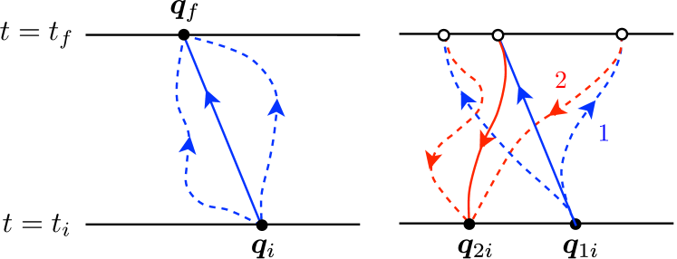
Doubling the degrees of freedom corresponds to the schematic on the right side of Fig. 1. The interpretation is that the variable evolves from some initial value at to the final time where upon is a value determined by the evolution, rather than specified with the problem. Likewise, for but taking on the value at the initial time. The arrows on the paths, or histories, corresponds to the integration direction for the integral of the Lagrangian. In particular, the arrows should not be confused with the direction that the doubled variables evolve through time, which is not yet determined.
The time integral of the Lagrangian is, of course, the action. The new action for the doubled variables, , can be written as
| (8) |
Notice that and are decoupled from each other. However, as with we may add an arbitrary function, , that does couple the doubled variables. More generally, the action above is given by
| (9) | ||||
This form defines a Lagrangian for the doubled degrees of freedom,
| (10) |
so that the action is
| (11) |
As with conservative mechanics, the Lagrangian is an arbitrary function of the doubled coordinates, the doubled velocities, and possibly time. Just as one can write (in certain coordinates Goldstein et al. (2002)) the usual Lagrangian as the difference of the kinetic and potential energies, where is an arbitrary function, so one can write as the difference of the conservative Lagrangians on the histories with an arbitrary “potential,” , on both histories.
We can determine some basic properties that should satisfy. A first property is that if were written as the difference of two functions, , then could be absorbed into the potential for each doubled variable leaving zero. If vanishes for a system then there may be no need to double the variables because the system is thus conservative.777That is, conservative up to any explicit time dependence in . However, one can derive by starting from a closed system and integrating out (or coarse graining) some inaccessible or irrelevant degrees of freedom to yield an open system for the accessible or relevant variables. Therefore, describes generalized forces that are not derivable from a potential energy (i.e., nonconservative forces) and necessarily couples the two histories with each other. One may thus regard as a nonconservative potential.
A second property is that must be anti-symmetric under interchanges of the labels . To see this, we note that the labels and are arbitrarily assigned to the histories in the right picture of Fig. 1. Since the resulting physics cannot change then the action should remain invariant under this exchange up to an overall irrelevant minus sign. This implies that
| (12) |
which equals if
| (13) |
Therefore, is an antisymmetric function of and and vanishes when .
We next find the conditions that ensure a well-defined variational principle under which the action is stationary. Both coordinate paths are parameterized as Galley (2013)
| (14) |
where are the coordinates of the two histories that makes the action stationary, are arbitrary functions of time denoting virtual displacements of the paths, and . In the usual formulation of Hamilton’s principle, there is one path and two conditions on its displacements, namely, that the latter vanish at the initial and final times. Here, we have two paths and so we need a total of four conditions to ensure that the variational principle is uniquely specified. As only initial data can be given for nonconservative systems we require that the variation of each path vanishes at the initial time so that . The remaining two conditions will follow from the variation of the action itself. The action in (11) is stationary under the variations in (14) if
| (15) |
which leads to
| (16) |
A subscript indicates that the enclosed quantity is evaluated at . The quantities are the canonical momenta conjugate to the doubled coordinates and defined through the nonconservative Lagrangian to be
| (17) |
where the first term on the far right side is the (conservative) conjugate momentum from (usually called ) and the second term is the part of the total momentum that comes from nonconservative interactions via . Similarly, the momentum for the second history is
| (18) |
The last line in (16) comes from integration by parts and will vanish if
| (19) |
From Fig. 1 we see that the variations at the final time are equal to each other so that
| (20) |
and thus the final conjugate momenta are also equal,
| (21) |
These two conditions together constitute the equality condition Galley (2013). The equality condition ensures that the boundary term from integration by parts in (16) will vanish for arbitrary variations provided only that the two histories agree with each other at the final time. The actual values of the variations are free, but whatever they are, the final states match at . Likewise, the conjugate momenta at the final time must agree with each other but are otherwise unspecified. This leads to the key point that the equality condition ensures that our variational principle is consistent with our ignorance of the final state of the accessible degrees of freedom. Indeed, it is unsatisfactory to fix the final configuration of the system in order to determine the equations of motion that are to be solved from initial data alone. The equality condition is thus a crucial ingredient in extending Hamilton’s principle to nonconservative systems.
The equations for both histories then follow by setting the integrand in (16) to zero for arbitrary variations, , which gives the two equations
| (22) |
where . However, the resulting equations are not necessarily physical until we take the physical limit (PL) wherein the histories are identified
| (23) |
after all variations and derivatives of the Lagrangian are taken. The PL of both equations in (22) reduces to
| (24) | ||||
where we have written the nonconservative Lagrangian in terms of its conservative piece and the function, and “PL” denotes taking the physical limit in (23). The right side on the first line comes from the physical limit of the equations while the second line from . Notice that these differ by an overall minus sign but are equal because is antisymmetric under interchanges of the labels .
A more convenient parametrization of the coordinates that yields some important physical insight is given by the average and relative difference of the two histories,
| (25) | ||||
| (26) |
The physical limit is then simply given by
| (27) |
Therefore, the average history is the physically relevant one that survives the physical limit while the difference coordinate simply vanishes. In these coordinates, the nonconservative Lagrangian is
| (28) |
It should be noted that cannot be written in the parametrization as in (10) but can be derived simply from (10). The equality condition in (20) and (21) is simply
| (29) |
implying that the physically relevant average () quantities are not specified at the final time in order to have a well-defined variational principle. Here,
The resulting equations of motion are easily found to be Galley (2013)
| (30) |
where now . Notice that this expression has the same form as in the parametrization in (22). This reflects a more general result that the nonconservative Euler-Lagrange equations are covariant (which is also true in conservative Lagrangian mechanics Goldstein et al. (2002); Scheck (1996)) with respect to the history indices. Therefore, the form of the nonconservative Euler-Lagrange equations does not depend on the specific choice of history labels.
Taking the physical limit of (30) is trivial. For we have that (30) is identically zero in the physical limit while the equations survive
| (31) |
Expressed in terms of and this yields
| (32) |
Here, is the generalized nonconservative force derived from . The structure of suggests that is a nonconservative potential function. Equation (32) is the Euler-Lagrange equations of motion for the nonconservative dynamics of , as derived with from the variational principle introduced in Galley (2013) consistent with giving initial data. We remark that these equations of motion are the same whether we choose to parametrize the histories by , , or another pair of labels because the action is invariant. We end by pointing out that (32) can also be derived by computing
| (33) |
where is a functional derivative with respect to . This expression is the more general form when higher than first derivatives of appear in a problem. We discuss in Appendix A how the variational principle of stationary nonconservative action changes when higher time derivatives are present.
II.3 Illustrative example revisited
With the framework in place to properly incorporate initial data and causal dynamics into a variational principle for the nonconservative action, let us now revisit the example from Sec. II.1 and check that this formalism gives the correct equations of motion for after eliminating from the original action. We assume initial conditions are given for both oscillators, namely,
| (34) | ||||
| (35) |
The two oscillators taken together form a closed system, which conserves the total energy, with an action given in the usual mechanics formalism by (1). We next integrate out from the action. However, we first double the degrees of freedom in the problem in order to ensure that the proper causal conditions on the dynamics of are respected and maintained. The resulting nonconservative action in the basis is
| (36) |
The fact that the total system is closed means that vanishes. Integrating out will turn out to generate a non-zero effective for the open system dynamics of .
The effective action for the open dynamics of is found by eliminating the variables from (36). The satisfy
| (37) |
We associate the initial conditions in (35) with the initial conditions for because the physical limit of at the initial time is just given by (35). The equality condition at the final time gives “final” conditions for given by
| (38) |
The resulting solutions to (37) are thus
| (39) | ||||
| (40) |
where is the homogeneous solution to the equation. The retarded Green’s function is given by
| (41) |
where is the Heaviside step function, and the advanced Green’s function is related through . Notice that because the solution to the (physical) equation satisfies initial data while the solution to the (unphysical) equation satisfies final data then the former evolves forward in time while the latter evolves , hence the appearance of the advanced Green’s function. This is a general feature of the parametrization. We comment that in the parametrization evolve both forward and backward in time, as can be easily shown from (39) and (40).
Substituting (39) and (40) back into the action in (36) yields the effective action for ,
from which we read off that
| (42) | ||||
Comparing with the effective action constructed using the usual Hamilton’s principle in (2) reveals that the last term above contains a factor that is not symmetric in and thus couples to the full retarded Green’s function, not just the time-symmetric piece. The resulting equations of motion for follows from (32) or (33) and gives
| (43) |
This is the correct equation of motion for , which can be easily verified by eliminating at the level of the equations of motion instead of at the level of the action. Importantly, solutions to (43) evolve causally from initial data and only the retarded Green’s function appears in the equation. Therefore, we have demonstrated that the nonconservative generalization of Hamilton’s principle presented in Sec. II.2 gives the proper causal evolution for the open system given only initial data and does not require fixing the configuration of the degrees of freedom at the final time in order to define the variational principle Galley (2013).
II.4 Noether’s theorem generalized
In conservative Lagrangian mechanics, Noether’s theorem Noether (1918) states that there exists a quantity conserved in time for every continuous transformation that keeps the action invariant when the Euler-Lagrange equations are satisfied. For example, time translation invariance and rotational invariance give rise to energy and angular momentum conservation, respectively. Quantities that are conserved in conservative mechanics may no longer be when considering open systems subject to nonconservative interactions. Therefore, Noether’s theorem must be modified. Nevertheless, the corresponding conservative action is still invariant under the original continuous transformations, and thus generates the same Noether currents. However, because the Euler-Lagrange equations are generally sourced by nonconservative forces in (32), then one will expect the Noether currents to change in a manner depending on . In this section, we show that this is indeed generally the case. More importantly, because we know how the nonconservative forces are derived from , we will find very useful expressions for the Noether currents and their changes in time that follow directly from .
Consider the conservative action given by
| (44) |
Let us assume that is invariant under the following infinitesimal transformations
| (45) | ||||
| (46) |
with
| (47) |
where is a small parameter with index associated with (the Lie algebra of) the symmetry group, which should not be confused with the history labels that will not appear in this section. Under these transformations the conservative action takes the form
| (48) |
which, by assumption, equals to the right side of (44) so that through first order in and the change in the conservative action is
| (49) |
Applying the product rule and rearranging gives
| (50) |
The first term is the total time derivative of the quantity
| (51) |
which is the value of the Hamiltonian and is called the energy function Goldstein et al. (2002). The first term on the second line of (50) is the current associated with the transformation in (46),
| (52) |
We may now use the Euler-Lagrange equations in (32) to write (50) in terms of , , and the non-conservative forces as
| (53) |
Finally, since and are independent then each factor in square brackets must vanish for the whole integral to vanish. The result is
| (54) | ||||
| (55) |
which follows from the invariance of the conservative action under the transformations in (45) and (46). In this sense, (54) and (55) can be viewed as a generalization of Noether’s theorem where instead of a conserved set of currents we have a set of equations that determines how these currents change with time in the presence of nonconservative forces and interactions. If is nonzero and the Lagrangian has no explicit time dependence then the energy and current will necessarily change in time. If vanishes then the energy and current are conserved in time and we recover Noether’s theorem for discrete mechanical systems. The derivation of (54) and (55) does not rely on the new framework discussed in Sec. II and is not new. What is new is that we know how depends on the nonconservative interactions in the action via from (32). This relation allows us to provide powerful alternative but equivalent expressions for (54) and (55).
We start with the energy equation in (54) and write out the nonconservative force from (32) explicitly in terms of as
| (56) |
Next, we note that the total canonical momentum is given by
| (57) |
The first term on the far right side is familiar as the part of the total canonical momentum that is associated with conservative actions while the second term is the part of that comes from the nonconservative interactions of the system,
| (58) |
Noting that we can bring the velocity in (56) into the square brackets. Doing so and using the product rule for the time derivative in the last term gives
| (59) |
after some rearranging. Similar manipulations turn the current equation in (55) into
| (60) |
The left sides of both (59) and (60) are total time derivatives of a shifted energy and current,
| (61) | ||||
| (62) |
The contributions that come from are corrections to the energy and current that result from the open system’s interaction with the inaccessible or eliminated degrees of freedom. We can regard and as the total energy and current of the accessible degrees of freedom including contributions from the nonconservative interactions. We will see a familiar example from radiation reaction in electrodynamics that confirms this interpretation in Sec. III.4. Our alternative expressions of Noether’s theorem generalized to nonconservative systems are thus given by
| (63) | ||||
| (64) |
and results directly from the generalized nonconservative forces being expressed in terms of a known and/or derived .
Equations (61)–(64) constitute some of the main results of this paper. These expressions indicate several interesting consequences. The first indicates that the total energy and Noether current of the accessible degrees of freedom include contributions from the nonconservative momentum . The second is that when is non-zero, the change in energy necessarily depends on the acceleration of the accessible variables, as seen in the last term of (59). Another key point is that (61)–(64) are computed directly from the nonconservative potential . Therefore, once is known then one can directly calculate how the energy and, for example, angular momentum of the system changes in time without having to perform separate calculations to explicitly compute these quantities.
As a final comment, if depends explicitly on then there can be an ambiguity concerning the interpretation of (61) as the total energy of the accessible degrees of freedom. This is best seen with a simple example. Choose , for constant , and , which is related to through integration by parts in the nonconservative action . One can show that the equations of motion are the same and the content of Noether’s theorem in (63) is the same using either or . However, the nonconservative conjugate momentum from vanishes () while has . Therefore, the corresponding energies and are different. The former is the correct expression for interpreting (61) as the total energy of the accessible degrees of freedom. However, one should recall that is often only just a coordinate, as opposed to a geometric quantity like a vector or a tensor. Hence, may not have the correct transformation properties whereas will. Therefore, to alleviate any ambiguity we believe it is useful to use the form of , not , for problems where the nonconservative potential depends explicitly on and/or . Such systems are studied in Secs. III.1–III.3. In all other cases when depends on time derivatives of then there is no such ambiguity (see Appendix A for including higher time derivatives in the formalism) as demonstrated in Sec. III.4. When integrating out a subset of variables from the full conservative problem, the resulting nonconservative potential will typically be of the form such that the shifted Noether currents are consistent with the appropriate physical interpretation.
II.5 Internal energy and closure conditions
Until now we have been considering discrete mechanical “open” systems where the energy dissipated into the inaccessible degrees of freedom does not feed back on the dynamics of the accessible variables. We may instead consider systems where such feedback could occur and affect the parameters of the accessible subsystem. A damped harmonic oscillator, for example, may heat up through friction and its natural frequency of oscillation or damping rate may change with the oscillator’s temperature. In this scenario, the energy lost from the accessible degrees of freedom by damping the oscillator goes into exciting the inaccessible microscopic degrees of freedom composing the oscillator.
If the “internal” energy of the inaccessible degrees of freedom plays a role in the dynamics of the accessible variables, then the equations of motion alone do not provide a closed set of equations because the internal energy evolution remains undetermined. We require additional information specified by the problem at hand to close the system of equations.
Systems where the energy of all inaccessible degrees of freedom can be accounted for by an internal energy carried within the Lagrangian can be considered “closed” such that the total energy is conserved. This closure condition, , also closes the system of equations, telling us how the internal energy must change with time so that all the energy transferred to and from the accessible degrees of freedom are accounted for via energy conservation.
In examples in thermal systems, it is convenient to parametrize the internal energy of the inaccessible degrees of freedom by a time-dependent entropy. We will discuss such closure relations below for examples in both discrete (Sec. III.3) and continuum mechanics (Sec. V.2.3). Such an approach is particularly useful in closed fluid systems, as we will see in Sec. V.2.
Other conditions to close the system of equations are possible, though these in practice will depend on the specifics of particular systems (see Sec. III.3 for an example including an external force). Since these closure conditions describe the energy evolution of the inaccessible degrees of freedom, they must be in general specified in addition to the variational principle that describes the accessible dynamics. Closure conditions are best illustrated through examples, as they depend on the the systems being modelled, as we will see in Sec. III and V.
II.6 On choosing
How does one choose or find the nonconservative potential for a problem of interest? There are several ways to answer this question. The particular answer one might choose will depend on the problem and its setup.
First, this question is similar to “How does one choose the conservative potential ?” in conservative mechanics. In some problems, one is either given a or one chooses the potential such that its gradient gives the desired force. Indeed, the situation is similar for . One may blindly prescribe , motivate the form of through some physical reasoning, or choose such that its derivatives in (32) give the desired nonconservative force.
Second, if one knows the nonconservative forces that appear in the equations of motion then one can reconstruct the corresponding , at least partially. This approach is useful for “non-Lagrangian” (or “non-Hamiltonian”) forces where a conservative Lagrangian (or Hamiltonian) cannot be found to generate some of the forces on the system. For example, note from (32) that is given by the pieces of linear in and . In particular, if is the nonconservative force on the system than simply writing as
| (65) |
guarantees that the correct force enters the Euler-Lagrange equations of motion in (32). Notice that we can only gain partial information about because we do not determine the higher order terms in the “” variables in this way.
Third, one may interpret the variables (when they are small) as being like virtual displacements. One can then regard as the virtual work done on the system by the inaccessible/irrelevant variables (whatever they may be) when displacing the system (evaluated in variables) through and/or . We use this approach in several examples below. We recall here the ambiguity associated with interpreting as the total energy of the accessible degrees of freedom for systems where depends explicitly on the generalized coordinates, , discussed in Sec. II.4.
Fourth, can be derived by integrating out a subset of degrees of freedom from a larger closed system. We showed an example of this already with the two coupled oscillators in Sec. II.3. In this case, one either knows what the full system is or has a sufficient model for it. However, it may be difficult to integrate out the irrelevant degrees of freedom exactly, in which case perturbative calculations in a suitable small parameter (e.g., coupling constant, ratios of length, time, speed, energy, or mass scales) tend to be useful.
Lastly, one can try to parametrize in a systematic fashion by imposing that the nonconservative action be invariant under the symmetries appropriate to the problem. Therefore, one can restrict terms into to those compatible with the symmetries. This is well-motivated from the the procedure of integrating out inaccessible degrees of freedom, where the resulting would have to be consistent with the underlying symmetries of the full system. This approach is inspired by the effective field theory framework (see e.g., Goldberger and Rothstein (2006)). However, in order for the resulting action to be predictive it is useful for there to be a naturally small expansion parameter that ensures only a finite number of terms will be included in for a given accuracy.
III Examples in discrete mechanics
While this new framework for nonconservative mechanics may seem unfamiliar it can be used in a similar way as the familiar action and Lagrangian for conservative systems. Perhaps the best way to see how to use the nonconservative mechanics formalism is through examples. In this section, we will apply the formalism to a range of discrete nonconservative systems including the familiar forced damped harmonic oscillator, RLC circuits, and radiation reaction on an accelerating charge.
III.1 Forced damped oscillator
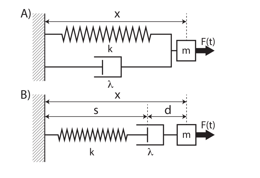
We first consider the familiar context of a forced, damped, harmonic oscillator. One physical realization of this system is shown in the top schematic in Fig. 2. Consider the following nonconservative Lagrangian where the conservative Lagrangian and nonconservative potential are given by
| (66) |
for some external forcing function . The conservative Lagrangian is simply that of a harmonic oscillator with mass and spring constant . If we substitute and from above into the nonconservative Euler-Lagrange equations in (32) then we find
| (67) |
which is the equation of motion for a forced, damped harmonic oscillator. The energy for the oscillator from (61) is
| (68) |
since, from (58), the nonconservative part of the total conjugate momentum vanishes, . The change in the oscillator’s energy is given by (63) here as
| (69) |
The first term corresponds to the power gained due to the external force, while the last term is the power lost due to damping.
III.2 The Maxwell element
In this example, we show how to use the nonconservative mechanics formalism for a problem with multiple but coupled degrees of freedom. This will also provide some background for the following example in Sec. III.3. This example is also interesting for generating an equation of motion that is a first order differential equation without implementing Lagrange multipliers.
Connecting a spring and a mechanical damper (e.g., a dashpot) in series yields a simple but ubiquitous description for modeling certain aspects in the rheology of visco-elastic materials under strain. This mechanical model, called a Maxwell element, is depicted by the lower schematic in Fig. 2. A Maxwell element can be seen in an everyday example of a door closer, which prevents it from slamming shut.
When an external force is applied the center of mass position, changes. Since is applied to the spring and the dashpot equally then the force that stretches the spring from its equilibrium position, , also goes into forcing movement through the viscous fluid in the dashpot by an amount . Therefore, we expect that
| (70) |
We take and to be the accessible degrees of freedom in the problem.
We take the conservative Lagrangian to be
| (71) |
The nonconservative potential will contain the work done by the external force in displacing the center of mass through plus the amount of energy lost by the system due to heating the viscous fluid in the damper, which we will model as being linear in the velocity of . Therefore, we propose
| (72) |
The equations of motion for are found from (32),
| (73) |
while that for are
| (74) |
and together are the equations of motion that we expect. If we write , as implied in Fig. 2, then we get the equivalent equations of motion,
| (75) | ||||
| (76) | ||||
Notice that we did not have to introduce a Lagrange multiplier to get the second equation of motion, which is a first order differential equation. We can solve for given the external force and some initial data, from which we can then construct the solution for and thus ,
| (77) |
Note that , and thus , depends on the integrated history of the elastic displacement of the spring alone.
III.3 Closure condition for the Maxwell element
In this example, we show how to derive a closure condition (discussed in Sec. II.5) for a Maxwell element to close the system of equations when the evolution of the accessible variables is affected by the internal energy of inaccessible degrees of freedom. Recall that a Maxwell element is damped by a viscous fluid in the dashpot. In the process, the damper may heat up and the damping coefficient may change value. Therefore, the mechanical energy of the Maxwell element is transferred to the internal energy of the viscous fluid as heat. The internal energy of a viscous fluid is naturally parametrized by the thermodynamic entropy assuming also an equation of state, , that does not depend on the generalized coordinates or velocities. With a given function of entropy we can write the nonconservative Lagrangian in (71) and (72) as
| (80) | ||||
| (81) |
The equations of motion are similar to those given in the previous example except that depends on time through the entropy of the viscous fluid in the dashpot,
| (82) | ||||
| (83) | ||||
with . The energy of the Maxwell element is given by
| (84) |
The change in the open subsystem’s energy is given by (63) as
| (85) |
With the inclusion of the damper’s internal energy, the total energy of the whole Maxwell element is given by . Therefore, if all of the energy supplied by the external force goes into changing then
| (86) |
Thus the energy dissipated by the dashpot goes into changing the internal energy , which is natural since the Maxwell element is a completely closed system aside from the external force acting on it. Therefore, the entropy must change with time according to the closure condition implied from (85) and (86), namely,
| (87) |
where we have defined temperature in the usual way. The closure relation thus gives the rate at which the damper is heated through viscous dissipation in the dashpot. Such a relation is needed if the internal energy of the dashpot changes with time in order to close the system of equations, which are given by (82), (83), and (87). Notice that if that the entropy changes in a way that satisfies the second law of thermodynamics. Furthermore, the right side of (87) is the amount of energy from heating that we would expect. That these results fall out naturally from our nonconservative framework is a powerful feature when discussing dissipative fluids, thermal diffusivity, and heat flow below in Sec. V.
III.4 Radiation reaction on an accelerating charge
Here we consider a system where the canonical momentum, in (58), associated with is non-zero and recover some well-known results in electrodynamical radiation reaction. As we shall see, being able to calculate from directly as well as its effects on observable quantities like energy and angular momentum is a very powerful feature of nonconservative mechanics.
The nonconservative Lagrangian describing the relativistic motion of an extended charge experiencing radiation reaction was derived in Ref. Galley et al. (2010) by integrating out the influence of the electromagnetic field on the motion of the charged body using effective field theory techniques.
For simplicity and pedagogical purposes, but without loss of generality, we work here in the nonrelativistic limit where the nonconservative Lagrangian from Ref. Galley et al. (2010) is expressed by
| (88) |
where is an external force that sets the charge in motion, , and . Reading off from (88), the conservative Lagrangian and nonconservative potential are
| (89) | ||||
| (90) |
The relativistic nonconservative Lagrangian with the leading order contributions from the charge’s finite size can be found in Galley et al. (2010). The equations of motion in the physical limit are found from (32) to be
| (91) |
which is the well-known Abraham-Lorentz-Dirac equation of motion for the point-like charge Jackson (1999). We will not discuss issues of runaway solutions associated with using a point-like charge to model the motion as this and related issues are outside the scope of this work. However, standard techniques for obtaining physically well-behaved solutions can be performed at the level of the equations of motion Landau and Lifshitz (1986a) and the action, which are commonly performed in effective field theories, through an order of reduction procedure that yields physically accurate solutions until quantum effects enter (see e.g., Koga (2004)).
The momentum associated with is non-zero,
| (92) |
Therefore, the total energy for a radiating, accelerated charge is given by (61) by
| (93) |
The second term in is the well-known Schott term and accounts for the energy of the near-zone part of the electromagnetic field that is not radiated to infinity. The Schott term arises precisely because of the charge’s nonconservative self-interaction that results from eliminating the electromagnetic degrees of freedom from the action. The corresponding canonical momentum associated with the Schott term is given simply by in (92). Note that choosing instead gives the same expression for the nonconservative conjugate momentum in (92) upon using the more general expression in (269). Therefore, either expression for the nonconservative potential gives the same expressions for physical quantities. The change in with time is given by (63),
| (94) |
The first term on the right side of (94) is the power radiated by the accelerated charge (derived by Larmor Jackson (1999)) and the second term is the power supplied by the external force to accelerate the charge in the first place.
From the paragraph following (63) and (64), the nonconservative part of the momentum will couple to the acceleration, which yields the Larmor contribution. However, this necessarily implies that the energy is shifted by contracted with the charge’s velocity. Therefore, the fact that the radiated power depends on the acceleration implies the existence of the Schott energy term as a contribution to the total energy associated with the dynamics of the charge. A key point is that the change in the energy of the system is derived directly from the new Lagrangian formulation without needing to apply any additional arguments about energy or balancing fluxes or performing a separate calculation for the radiated field (see e.g., Jackson (1999)).
The transformation of the conservative action under a rotation through a small angle about the direction ,
| (95) |
implies that the total angular momentum components in (62) are
| (96) |
Like the total energy, the total angular momentum receives a correction from the interaction between the charge and the electromagnetic field, which can be interpreted as the angular momentum from the field in the near zone that is not radiated to infinity but carried along with the charge as a whole. The change in time of is the torque on the charge and is given in (64) by
| (97) |
The torque on the charge is thus driven by the acceleration and the external force.
III.5 Linear RLC circuits
In this final example, we show that the nonconservative formalism discussed in Sec. II can be applied to non-mechanical systems such as circuits.
Circuits consisting of only energy-conserving elements (e.g., inductors and capacitors) may be described by a standard variational formulation Ober-Blöbaum et al. (2013). However, with the variational principle discussed in Sec. II we may also describe dissipative elements (e.g., resistors). Though we focus here on linear circuit elements there is no obstacle to including nonlinear ones (e.g., transistors).
Figure 3 shows an example circuit composed of a resistor, inductor, and capacitor. The degrees of freedom in this problem are the net charges that have flowed through elements . The corresponding generalized velocities are the currents, . However, the variables are not all independent because there are Kirchoff constraints to be applied. The number of independent net-charges is actually the number of loop currents in the whole circuit. These independent degrees of freedom are denoted by for . Then each is a directed sum of the of the independent charges flowing through the loop currents,
| (98) |
where is a constant of integration, denotes those which go through , and is negative if the currents and are oppositely oriented.
There are then two approaches to constructing the action for a circuit. One may impose the constraints of (98) by inserting Lagrange multipliers. Alternatively, since we are here only dealing with linear elements, we may directly write the ’s as functions of ’s and be assured of the same dynamics.
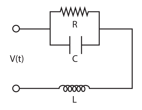
The circuit in Fig. 3 requires two current loops and thus two independent net-charges, and . Take current to flow through the – loop in the clockwise direction and current to flow through the –– loop in the clockwise direction. This gives three relations,
| (99) | ||||
| (100) | ||||
| (101) |
where is a constant of integration denoting the charge on the capacitor at time (alternatively, this constant may be absorbed into and/or ).
The conservative Lagrangian and nonconservative potential are taken to be
| (102) | ||||
| (103) | ||||
| (104) |
The “kinetic energy” in an inductor is , while the potential energy stored in a capacitor is . These two terms constitute the conservative Lagrangian. Meanwhile, is composed of two terms. The first comes from the energy associated with the external voltage acting on the amount of charge flowing through the –– loop. The second is the amount of energy lost by heating the resistor.
A straightforward calculation shows that this clearly reproduces Kirchhoff’s voltage law about each loop. In particular, the variations with respect to and yield
| (105) |
upon using (99)-(101) where and . Note that this nonconservative action formalism can also be easily applied to circuits with nonlinear elements and with more elements than we considered in this example.
IV Nonconservative classical field theories
We have seen that discrete nonconservative systems can be modeled through nonconservative actions and the variational principle described in Sec. II, and explored several examples of such systems in Sec. III. In the remainder of this paper we will extend this formalism to include nonconservative continuum mechanics and classical field theories (Sec. IV), followed by several example applications (Sec. V), with particular focus on continuum mechanics. In what follows, we will often use “continuum mechanics” and “field theories” interchangeably.
Consider fields where labels the components whose evolution is to be studied for times in and within a spatial volume , such that , where . For example, may represent the electromagnetic vector potential , which is a relativistic field (where is the space-time indices) that transforms as a vector under Poincare transformations. For a field undergoing nonconservative interactions, we must double the degrees of freedom as we did for discrete systems, in which case , in order to capture the appropriate nonconservative (e.g., dissipative) effects and account for the correct causal evolution of the open system dynamics.
IV.1 Lagrangian mechanics
The action for doubled variables is given by
| (106) |
where is the space-time volume of interest and is the nonconservative Lagrangian density and, as with the discrete conservative Lagrangian , is an arbitrary function of the doubled fields, their derivatives, and possibly the space-time coordinates ,
| (107) |
Recall that for certain coordinates the usual Lagrangian can be written as the difference of the kinetic and potential energies. Likewise, for certain history labels the new Lagrangian density can be separated into its conservative and nonconservative pieces as
| (108) |
Note that, in general, is an arbitrary function of the doubled variables and does not necessarily have the form on the right side of (108) in a general set of canonical coordinates.
One such set of coordinates is provided by the basis, defined by
| (109) |
For generality, we label the doubled fields by a lower case Roman letter from the beginning of the alphabet, . To vary the action we let
| (110) |
where and are arbitrary functions of . The fields evaluated at are taken to be the ones for which the action is stationary with respect to changes in . Substituting (110) into (108) and expanding out the action in (106) through first order in gives
| (111) |
where indicates that the quantity inside the brackets is evaluated at and we implicitly sum over the index. Integrating by parts on the terms gives
| (112) |
where is the boundary of the spacetime volume and is a surface area element on pointing out of .
As in discrete mechanics, if the boundary of the space-time volume is fixed then there should be no contribution to the action’s variation. For notational convenience, we define the current densities as
| (113) |
in the basis and
| (114) |
in the basis. These expressions can be condensed by the introduction of a “metric” that can be used to raise and lower the history indices. In the labels the metric is and in the labels is so that (113) and (114) are given succinctly as
| (115) |
In discrete mechanics the equality condition for the variations at the final time () and the vanishing of at the initial time guarantees that the boundary terms do not contribute to the variation. In continuum mechanics, we instead have a spacetime volume with a boundary . When describing nonconservative field theories, which are necessarily ones that can evolve with nonequilibrium or nonstationary dynamics, one has to solve the equations of motion from a set of initial data specified at to a final time . If denotes a spatial -volume with boundary then the surface integrals in (112) take the following form,
| (116) |
where
| (117) |
is the momentum canonically conjugate to . In the coordinates this equals
| (118) | ||||
Generalizing Fig. 1 to field theories implies that at the initial time the variations individually vanish,
| (119) |
for . In addition, the variations at the final time are equal so that the quantity in brackets in (118) vanishes if we take the continuum version of the equality condition introduced earlier, namely,
| (120) |
for . We are thus left with the surface integrals over ,
| (121) |
With the following two conditions, the surface integrals for non-dynamical boundaries will vanish:
| (122) | |||||||
| (123) |
For certain problems, we can better justify these conditions by analogy with discrete mechanics. For example, if the satisfy a linear, homogeneous, second order PDE, then (120) uniquely determines in the past domain of dependence of (the spatial volume at ). The vanishing of would be extended to the entire interior of by giving conditions (122)-(123). Then, just as in discrete mechanics, we find that the minus variables vanish throughout the entire solution.
The variation of the action is then given by , which is stationary when
| (124) |
and is satisfied for any provided that
| (125) |
In the physical limit (“PL”) all “” variables vanish and all “” variables take their physical values and describe the accessible degrees of freedom. This means that, in the basis, only the equation with survives because that equation takes derivatives with respect to the “” variables and so only the terms in that are perturbatively linear in the “” variables will contribute in the physical limit, giving
| (126) |
which can be written in terms of and as
| (127) |
All of the results in this section can be extended to fields on a curved background space-time in a straightforward manner following standard techniques (see e.g., Misner et al. (1973)).
Finally, choosing or finding for a specific problem can be accomplished using the approaches (and possibly others) discussed in Sec. II.6.
IV.2 Noether’s theorem generalized
We show here how Noether’s theorem is generalized due to nonconservative forces and interactions. Many of the manipulations are similar to those encountered for discrete mechanical systems in Sec. II.4. Consider the transformations,
| (128) | ||||
| (129) |
with
| (130) | ||||
| (131) |
and and are small parameters associated with (the Lie algebras of) the symmetry groups in question that keep the following conservative action invariant
| (132) |
The index in (131) should not be confused with the history labels, which will not appear in this section. The invariance of the action implies, using similar manipulations as in Sec. II.4, that
| (133) |
Rearranging terms using the product rule for partial derivatives gives
| (134) |
The quantity
| (135) |
is the canonical stress-energy-momentum (or simply stress) tensor. The Noether current density associated with coordinate transformation (128) appears in the first divergence term of (134), given by
| (136) |
The first term on the last line of (134) is the Noether current density associated with the transformation in (129),
| (137) |
We may now use the Euler-Lagrange equations of motion in (127) to write (134) in terms of , , and as
| (138) |
Finally, since and are independent then each factor in square brackets must vanish for the whole integral to vanish. The result is
| (139) | ||||
| (140) |
We see that a nonzero and explicit dependence of the Lagrangian density source (or drain) the system’s Noether current. Once is known, through a calculation from integrating out degrees of freedom, coarse-graining, or otherwise specified, one may calculate how the Noether current changes for the accessible degrees of freedom. That is, once the nonconservative action is known one can compute how energy density, angular momentum density, etc., changes (see below). For a closed system having conservative interactions, the nonconservative generalized interactions vanish, , and we recover Noether’s theorem.
A more convenient but equivalent form for the divergences in (139) and (140) is found using similar manipulations as performed for discrete systems in Sec. II.4. We quote the result here, which is
| (141) | ||||
| (142) |
where
| (143) |
is the part of the total current density that is associated with nonconservative interactions. The left sides are the divergence of a shifted current densities defined by
| (144) | ||||
| (145) |
The contributions that come from are corrections to the stress-energy and current density that result from the open system’s interaction with the inaccessible or eliminated degrees of freedom. We can regard and as the total stress-energy and current density of the accessible degrees of freedom that include contributions from nonconservative interactions. Our alternative expressions of Noether’s theorem generalized to nonconservative field theories are thus given by
| (146) | ||||
| (147) |
For Lagrangians with space-time translation symmetry, generated by , we find the expression for the divergence of the total stress tensor,
| (148) |
For various reasons, the canonical stress-energy tensor or are not necessarily the preferred quantities for calculating the energy, momenta, and fluxes of fields. For example, the canonical stress-energy tensor does not source gravitational fields in almost all theories of gravitation, including general relativity. As another example, the canonical stress-energy tensor is not gauge invariant in electromagnetism because space-dependent gauge transformations do not commute with spatial translations. In concluding this subsection, we mention that the standard techniques for building a symmetric stress-energy tensor from follows in the same way as for conservative field theories. These manipulations also carry through for making a symmetric nonconservative stress-energy tensor from . Finally, the divergences of and (or and ) are the same and equal the right hand side of (148) (or (139)). For more details, see Soper (2008); Goldstein et al. (2002); Jackson (1999), for example.
Equations (144)-(148) constitute some of the main results of this paper. As in discrete mechanics, there are several interesting consequences. The first indicates that the total stress, energy, and momenta of the accessible degrees of freedom include contributions from the nonconservative current density . The second is that when is non-zero that the divergence of the stress-energy tensor necessarily depends on two derivatives of the accessible field variable, as seen in the last term in (148). Another key point is that (144)-(148) are computed directly from the nonconservative potential density . Therefore, once is known then one can directly calculate how the stress-energy tensor and Noether current density change with time without having to perform separate calculations to explicitly compute these quantities.
IV.3 Internal energy and closure conditions
In our previous discussion of nonconservative discrete mechanics we considered systems where the energy contained in the inaccessible degrees of freedom, the “internal” energy, could feed back into the dynamics of the the accessible subsystem. Such systems required a closure condition, in addition to the variational principle that determines the dynamics of the accessible degrees of freedom, in order to close the system of equations and allow for the system to be solved. In this section, we consider the internal energy density and closure conditions for continuum systems.
In continuum mechanics, accessible degrees of freedom are often generated through coarse graining procedures, where the the “fast” or “microscopic” degrees of freedom are treated as inaccessible, while macroscopically averaged, or “slow” quantities become the accessible degrees of freedom. In such systems, the energy contained in the inaccessible degrees of freedom are often included in the internal energy density, which may be related to local thermodynamic parameters like density and entropy through an equation of state. If we had access to the full conservative Lagrangian of the system, , including all microscopic degrees of freedom and their interactions, then, in the absence of external forces, the total energy would be conserved such that the divergence of the full conservative stress-energy tensor would have zero time component
| (149) |
For some coarse-grained systems we can include an internal energy density in the Lagrangian, , that accounts for all of the energy of the microscopic inaccessible degrees of freedom, such that the system is closed. The total nonconservative stress-energy tensor then includes the contributions from the inaccessible momentum flux as well as the energy in the inaccessible subsystem, allowing us to equate the time component of its divergence with that of the full stress-energy tensor
| (150) |
which we take to be the closure condition for closed continuum systems.
As in the discrete case, other conditions to close the system of equations are possible, though these in practice will depend on the specifics of particular systems. We illustrate through specific examples in Sec. V.
V Examples in field theory
To show how to use our new formalism for nonconservative classical field theories that we have developed in the previous section, we provide several examples, starting with a simple example of coupled scalar fields, which serves as an analog of the two-oscillator example from Sec. II. One of the most useful properties of action formulations is the ability to construct actions additively for various interactions and fields. In this spirit we next explore several example physical systems starting with a simple perfect fluid, then developing and adding action terms describing various interactions, through the nonconservative potential . These include heat diffusion, viscous dissipation, and viscoelasticity.
V.1 Two coupled scalar fields
Consider two relativistic scalar fields, and , nonlinearly coupled to each other and mutually evolving in a flat spacetime from initial data specified at a given instant of time. The action for this (closed) system is
| (151) |
where is a coupling constant and with and the Minkowski metric in rectangular coordinates. We choose to integrate out the field at the level of the action. Often such a choice would be motivated by the physics of the problem or the relative scales but our choice is motivated by pedagogy.
Upon doubling both fields and choosing to work with the representation, the nonconservative action is
| (152) |
The equations of motion for are linear,
| (153) |
where . Just as in the discrete example with two harmonic oscillators in Sec. II.3, the equation is solved using the retarded Green’s function since the initial data is non-trivial in the physical limit while the equation is solved with the advanced Green’s function since the data at the final time is fixed by the equality condition. Therefore,
| (154) | ||||
| (155) |
where is a homogeneous solution. Note that has no homogeneous contribution because we are solving a second order partial differential equation with trivial final data. Substitution of these solutions back into (152) gives the nonconservative effective action for ,
| (156) |
from which we read off that
| (157) | ||||
| (158) |
The equations of motion for follow by varying with respect to or by applying (127) to the equations directly above. Both calculations give the same result,
which depends on the past nonlinear evolution of and is the correct equation one would have found by integrating out at the level of the equations of motion.
For further examples in relativistic field theories, see Galley and Leibovich (2012) for integrating out radiative gravitational perturbations in the post-Newtonian approximation for the compact binary inspirals due to the emission of gravitational waves. See also the interesting work of Kevrekidis Kevrekidis (2014) who applies nonconservative field theory with the collective coordinate Dauxois and Peyrard (2006) (or variational Malomed (2002, 2006)) method to find very accurate and practical approximate equations of motion and solutions for nonlinear wave propagation in dissipative sine-Gordon and models.
V.2 Hydrodynamics
An extensive class of classical field theories can be found in problems in hydrodynamics, which are pervasive throughout many disciplines and applications. Many fluids of theoretical and practical interest are dissipative (e.g., viscous friction) and involve transport processes (e.g., heat diffusion) that are indicative of fluids in thermodynamical non-equilibrium. In this section we will develop nonconservative actions for classical hydrodynamics, including irreversible processes.
Andersson and Comer Andersson and Comer (2013), have recently begun to develop a relativistic description of hydrodynamic dissipation and heat transport using a constrained convective variational principle (see e.g., Prix (2004)), based on geometric considerations and the interaction of lower dimensional matter-space fields, without requiring a near equilibrium expansion.
Another recent approach to describe dissipative fluids is with effective field theory techniques Endlich et al. (2013); Grozdanov and Polonyi (2013) where viscous effects are included in the action via a perturbative derivative expansion of fluid elements in their comoving frame with respect to a stationary background flow. While these methods show promise for being guided by the underlying symmetries of the problem they seem to be inapplicable to non-smooth background flows (e.g., turbulence and shocks).
Here we adopt a more pragmatic approach and seek to construct actions, using our nonconservative formalism, transparently in familiar variables to reproduce well-known results in classical hydrodynamics that are useful for practical applications.
In the Eulerian description (see Appendix C) actions for perfect fluids often require a relatively large number of constraints (via Lagrange multipliers) to impose conservation of entropy, mass density, Lin number, etc. (see e.g., Ray (1972)). Additionally, one takes the mass and entropy densities as dynamical degrees of freedom, which is awkward since these quantities are merely functions that characterize and track some average properties of the coarse-grained microscopic variables comprising the fluid element. For example, one does not vary the action for a free particle with respect to its mass in addition to its position. While the Eulerian description of fluids will be more familiar to most readers, it is far easier to construct actions for fluid dynamics without constraints in the Lagrangian description (see e.g., Eckart (1960); Katz (1961); Seliger and Whitham (1968); Morrison (1998)).
In Lagrange coordinates (see Appendix C), a fluid element with label (for material-space indices ) traces a path in time with coordinates (for Eulerian-space indices ). Therefore, the fluid as a whole is a field over the coordinates with three scalar component functions indicating the coordinate of a piece of the fluid at time and label . We take this field as the dynamical degree of freedom for a fluid. In doing so, we are implicitly coarse-graining the large number of microscopic degrees of freedom associated with the individual molecules/atoms comprising the fluid.888We assume that the fluid’s microscopic degrees of freedom become thermalized at a much faster timescale than that of the fluid elements’ trajectories, which are a set of collective variables that arise from a coarse-graining procedure. We also implicitly assume that the coarse-graining procedure has introduced an entropy parameter that parametrizes the fluid elements’ internal energy. The field only captures some of the relevant or accessible degrees of freedom and constitutes a set of collective variables that are effectively open because the kinetic energy of a fluid element may be transferred to heat energy, which is a thermodynamic (or collective) accounting of the change in the average velocity of the molecules of the fluid element. In the examples that follow, we build actions for the dynamics of and additional thermodynamic quantities as befits the system in consideration. We also assume a single-species fluid for simplicity, though this can be straightforwardly generalized. See Appendix C for further discussion.
We now discuss constructing actions for fluids that exhibit nonconservative processes, which may include viscous dissipation and heat diffusion. Before studying more complicated problems involving heat fluxes and/or viscous dissipation, we begin by reviewing the action for an adiabatic inviscid (e.g., perfect) fluid. We refer the reader to Appendix C for the language and notation we use in the following examples.
V.2.1 Perfect (Inviscid and Adiabatic) Fluids
If a fluid element is in local thermodynamic equilibrium we can write the internal energy density (per unit Eulerian coordinate volume) as where , the Eulerian entropy density, and , the Eulerian mass density, are volume densities of the extensive thermodynamic variables. The differential of is then
| (159) |
where the local chemical potential (per unit mass), , and the local temperature are the intensive thermodynamic variables.
For a perfect, isentropic fluid with no viscosity or heat transport a conservative Lagrangian density can then be written as (we roughly follow the action formulation of Morrison (1998) for a perfect fluid)
| (160) |
where the time independent mass density for a particular Lagrangian label is and we have defined
| (161) |
Both and transform as scalar densities of weight , and therefore so does . Since there is no heat generation or heat transport the entropy density for a particular Lagrangian coordinate label is similarly time independent and given by . In addition, there are no dissipative or nonconservative processes here so .
The conservative action is constructed from as
| (162) |
The equations of motion for a fluid element’s path follow from (127) with . A straightforward calculation yields
| (163) |
where we have recalled the identity from (302), and defined the pressure (also a scalar density of weight ) by999This expression for pressure arises from the extensivity of the energy , entropy , volume , and particle number in a thermodynamic system, which generates the relation for a single species fluid where is the mass per particle and is the particle number.
| (164) |
In deriving (163) we have been careful to account for the fact that and have non-vanishing gradients of so that gives a contribution. The details of the full calculation are given in Appendix D. We recognize from (340) and (314-315) that the first two and last two terms in (163) combine to give covariant derivatives, and , respectively,
| (165) |
with . Equation (165) can be written in the more familiar Eulerian form
| (166) |
using (322). For rectilinear coordinates in flat space such that we have
| (167) |
The continuity equation is expressed in the Lagrange coordinates simply as . Applying (334) to this we obtain the continuity equation in Eulerian variables,
| (168) |
From the Lagrangian density in (160), the canonical stress-energy tensor for the perfect fluid has -coordinate components given in (144) by
| (169) | ||||
where .
The time component of the stress-energy tensor divergence in (148) yields the energy equation in Lagrangian variables for a perfect fluid,
| (170) |
where we note that does not depend explicitly on time, . We also remark that, after some manipulation, the energy equation can be written in a manifestly covariant form. Calculating the derivatives and using the continuity equation, , gives contracted with the equations of motion in (165). In Eulerian form the equation above is
| (171) |
where the quantity is the fluid’s enthalpy density. These expressions agree with those given in standard texts (see e.g., Landau and Lifshitz (1986b); Batchelor (1967)).
The spatial components of the stress-energy tensor divergence in (148) yield
| (172) |
where it is important to note that does depend explicitly on through the functions and . After some manipulation we find that the above equation equals the (manifestly covariant) equations of motion in (165) contracted with .
V.2.2 Viscous Isentropic Fluids (The “Cold Stone” Limit)
Next, it is instructive to consider the action for a locally isentropic viscous fluid in an “open” system such that all heat generated by viscous dissipation is removed through some external mechanism,101010We refer to this rather artificial, but pedagogically useful, system as the “Cold Stone” limit of a viscous fluid, in tribute to the “Cold Stone Creamery” chain of ice-cream dispensaries, where viscous (yet delicious) fluids are routinely mixed in thermal contact with a heat sink. such that .
We can account for the leading effect of viscous dissipation through in a couple of different ways. First, we can appeal to the concept that the “” variables can be interpreted as a kind of virtual displacement and identify as the work done on the fluid element by viscous friction when it undergoes a small virtual strain of . Second, we can consider linear combinations of the strain rate tensor and the strain tensor (see App. C.4 for definitions) along with constants giving a scalar density with units of energy per unit volume. In either case, we have111111We choose this as the lowest order dissipative term since terms with will yield diffusion-type processes, as we will see in Sec. V.2.4 when considering heat diffusion.
| (173) | ||||
| (174) |
where the viscous stress tensor for an isotropic viscous stress can be modeled by
| (175) | ||||
| (176) |
and
| (177) |
is the projection tensor that converts arbitrary rank- tensors to symmetric and trace-free ones. The coefficients in (175) are the dynamic or shear viscosity, , and the bulk or volume viscosity, , which are both scalar densities (weight +1) and may generally be functions of position and the local thermodynamic variables. Anisotropic viscous stress will have a more complicated form for .
In Eulerian coordinates the stress tensor transforms as a tensor density giving
| (178) | ||||
| (179) |
where and are scalar densities that transform such that the kinematic viscosities in each coordinate system are the same, and . The transformation between the Eulerian and Lagrangian stress tensor components is given by
| (180) |
The equations of motion for our “Cold Stone” fluid can be found from (127). Since is identical to that of the perfect fluid, its contribution to the equations of motion is the same as in (165). However, the nonvanishing gives rise to a dissipative force on the fluid element.
With
| (181) | ||||
we expand in to find
| (182) |
The non-conservative terms of the equations of motion (127) are given by
| (183) |
where are the Christoffel connection coefficients in Lagrangian coordinates, given explicitly in (317). This gives the the equations of motion for the ‘Cold Stone’ fluid,
| (184) |
which are equivalent the Navier-Stokes momentum conservation equations. Note that we have already computed the left side of (184) in the previous subsection. In the Eulerian coordinates this becomes
| (185) |
For rectilinear Euler coordinates in a flat space these become
| (186) |
which is the familiar form of the Navier-Stokes equations of motion for viscous fluid flows. Note that we used (307) and (180) in arriving at this form.
The canonical stress energy tensor when including nonconservative interactions is given by (144) such that
| (187) |
The spatial components of the divergence of the total stress-energy tensor (148) once again yield the equations of motion (184), while the time component gives
| (188) |
which is the energy equation for our “Cold Stone” fluid. In the Euler coordinates this can be written as
| (189) |
where the first term inside the divergence, , we recognize as the energy flux due to the mass transfer of the fluid, while the second term is the energy flux due to viscous shear. The right hand side is simply the rate of energy loss due to viscous dissipation.
V.2.3 A Viscous Perfectly Insulating Fluid
We now consider a viscous fluid that has perfectly insulating fluid elements, such that no heat diffusion is allowed between adjacent fluid elements. The system is “closed” such that viscously dissipated energy is deposited as heat into the fluid elements, in contrast with the open system described in the Cold Stone case. To do this we relax the condition on the entropy field, allowing it to explicitly depend on both time and the local fluid coordinate, such that , noting that the second law of thermodynamics requires that . This acts as an explicit time dependence in the Lagrangian, which can be viewed as an externally specified function that does not depend on the dynamical degrees of freedom .
The Euler-Lagrange equations give equations of motion for that are the same as for the Cold Stone case in (165). We also recover the continuity equation in (168). As noted in Sec. IV.3 the equations of motion and the continuity equation are no longer enough to “close” the system of equations. In general, we need an additional equation describing the evolution of the entropy , which must be specified in addition to the variational principle. We shall show that this comes about through a “closure relation.”
Consider the zeroth component of the divergence of the total stress tensor, namely, with space-time index in (148),
| (190) |
Note that the Lagrangian density has an explicit time dependence through the entropy, , such that
| (191) |
Since this fluid is a closed system, (see Sec. IV.3) we expect all energy dissipated from the accessible degrees of freedom to go into the internal energy such that the total energy is conserved. We then apply the closed system closure condition , which gives the energy and entropy equations
| (192) | |||
| (193) |
which can be written in terms of the Eulerian coordinates
| (194) | |||
| (195) |
Thus we see that entropy is generated by the irreversible viscous dissipation, and that the second Law of Thermodynamics, , requires that the coefficients and in the viscous stress tensor be positive.
We note that the open isentropic system condition, , and closed system condition, , are not the only ways to close the system of equations. Other systems can be specified giving different entropy and energy equations. We could imagine, for example, some fixed fraction of the energy going into the internal energy of the fluid while the rest escapes to external inaccessible degrees of freedom, or an isothermal condition on the fluid specifying the energy and entropy equations by a fixed temperature condition. For the simple fluid systems that follow, however, the most useful condition is the closure condition , which allows us to recover the expected behavior for the isolated fluid system, where the inaccessible degrees of freedom are only the microscopic coarse-grained degrees of freedom that contribute to the internal energy.
V.2.4 Inviscid Fluid with Heat Diffusion
To consider a fluid with heat diffusion we adopt the approach of Prix Prix (2004) and Andersson and Comer Andersson and Comer (2010) who treat the entropy as an auxiliary massless fluid, with its own degrees of freedom. Here we will take the labels of the entropy ‘fluid’ to be auxiliary degrees of freedom, which will have components labeled by the indices . This is equivalent to treating the diffusive heat flux as a separate degree of freedom. We can then construct a Jacobian matrix and determinant . We also have the inverse Jacobian , where is the cofactor matrix. Again, this assumes that the Jacobian is non-zero and we are in regions free from shocks. We can also express the metric in the coordinates that we can use to raise and lower the indices,
| (196) |
The mass density and velocity of the material are not directly affected by the perturbations of the entropy fluid label . However, the entropy density is now given by
| (197) |
where the denotes the entropy density in the coordinates. As in the closed system above, we allow the entropy density to be time dependent even in the coordinates, such that . Here, the second law of thermodynamics requires that we have locally .
The velocity of the entropy fluid is given by
| (198) | ||||
| (199) |
where and ) are the material and Eulerian coordinate positions, respectively, of the entropy fluid element labeled by coordinates . We can utilize the relative velocity identity (295) to write
| (200) |
which gives
| (201) |
and defines the relative velocity, such that
| (202) |
Consider the Lagrangian and density for a fluid with isotropic heat diffusion given by
| (203) | ||||
| (204) |
where is a scalar density of weight that is related to the thermal resistivity (see below) and may in general depend on time, position and the local thermodynamic variables. For more general anisotropic heat diffusion, we can replace the scalar density with a tensor density. We also note that , since near the physical limit, the minus variables are elements of a vector space. The expression is shorthand for , which is geometrically well defined.
The equations of motion for , obtained by varying with respect to , remains unchanged from that of the perfect fluid in (166) and the continuity equation (168).
To get the equations of motion for the entropy fluid we vary the nonconservative Lagrangian with in (127) and simply find
| (205) |
We have used the fact that is a scalar (and not a scalar density) to write .
We can define the Eulerian diffusive heat flux density to be
| (206) |
which transforms as a vector density of weight , such that
| (207) | ||||
| (208) |
The equation of motion (205) can then be rearranged to give,
| (209) |
which simply has Eulerian form
| (210) |
This is simply Fourier’s law of heat conduction where the scalar density is the thermal conductivity of the material. The thermal resistivity of the material is defined to be the inverse of the conductivity .
The components of the canonical stress-energy tensor are
| (211) | ||||
where, in the last line, we recognize as the Gibbs free energy density. Note that the nonconservative piece, , vanishes so that since for this system.
We can then write the divergence of the stress-energy tensor as
| (212) |
Note that the right hand side has no contributions from derivatives with respect to or . The spatial components of the divergence give the sums of the equations of motion for the and degrees of freedom, while the time component of the divergence yields
| (213) |
Combined with the closure condition, , the time component gives the energy equation
| (214) |
and the entropy equation
| (215) |
V.2.5 Navier-Stokes with Heat Flow
We are now prepared to construct an action to generate the full equations of irreversible fluid dynamics, including the effects of viscosity, heating, and heat diffusion. The action for a Navier-Stokes fluid with heat conduction is given in terms of and by
| (221) | ||||
| (222) |
where, as in the previous section and following Prix (2004); Andersson and Comer (2010), are the Eulerian coordinates of an entropy element labeled by such that .
As before we choose and to be the degrees of freedom. We also fix the mass density of the material fluid to the flow of the -coordinates, , but allow the entropy density to have an explicit time dependence with respect to the -coordinates. Notice that in (222) is given by the sum of the nonconservative potentials in (174) and (204). Furthermore, the first contribution in (222) is independent of the entropy fluid.
From (221) and (222), we can obtain the equations of motion for a viscous fluid with heat diffusion. Variation with respect to yields the Navier-Stokes momentum equations given already in (185),
Likewise, gives the continuity equation in (168),
Finally, variation with respect to yields the diffusive heat flux density in (206)
which is an expression of Fourier’s law of heat conduction. Notice that the additivity of the viscosity and heat diffusion pieces in have allowed us to recycle previous calculations for deriving the equations of motion.
The components of the nonconservative stress-energy tensor are found to be
| (223) | ||||
The last two terms in and are contributions coming from the nonconservative effects of viscosity, heating, and heat diffusion, and arise because defined in (143) is non-zero.
The divergence of the total stress-energy tensor gives for the th component,
| (224) |
Combining this with the closure condition, , gives the energy equation,
| (225) |
and the entropy equation
| (226) |
Remarkably, we have been able to generate the entropy evolution equation for a non-equilibrium thermodynamic system by simply using the nonconservative variational principle, and the closed system closure condition. We expect our formalism to apply equally well to other non-equilibrium coarse-grained systems where the (effectively open) accessible degrees of freedom can be described by a nonconservative action that accounts for the energy of the microscopic degrees of freedom that have been coarse-grained out. This allows us capture the thermodynamics of generic non-equilibrium systems using an action principle formulation.
V.3 Microhydrodynamics and movable boundaries
We next consider a system where dynamical boundary effects can be expected to dominate. The effect of such boundaries are considered in App. B for deriving the nonconservative Euler-Lagrange equations of motion and generalizing Noether’s theorem.
In some applications, a liquid fluid may contain extended objects that are very small compared to the typical length scales of the fluid as a whole. These particles compose the suspension microstructure of the fluid and thus their dynamics is important for many applications, especially industrial ones. From a practical point, the particles tend to vary between and hundreds of microns in size Kim and Karrila (1991) and can have very complicated geometries, which may evolve dynamically in time as is the case with microscopic biological swimmers.
If and are the typical velocity and length scale, respectively, of a small particle in a fluid with mass density and (dynamic) viscosity then the Reynolds number is given by
| (227) |
At small length scales and low velocities, the effects of viscosity dominate the particle’s evolution so that , which is called the Stokes regime or limit. Therefore, the kinetic energy of the fluid’s motion generated by the particle will be much smaller than the internal energy of any fluid element.
Starting from the action for a viscous fluid with heat flow from Sec. V.2.5, we recall from (221) and (222) that the conservative Lagrangian and nonconservative potential densities are
The ratio of the viscous part of to the inertial part of scales like . Likewise, the inertial energy density of the fluid is much smaller than the internal energy density because the particles move slowly in the viscous-dominated regime. Following Kim and Karrila (1991), we also assume that the fluid is thermally well equilibrated and the heat flow is negligibly small on the length scales relevant to micro-hydrodynamical processes. We also assume the heating due to dissipation is much smaller than the internal energy. Consequently, we take the entropy density to be time-independent and the fluid to be isothermal. Likewise, the change in the density under these conditions is negligible so that the liquid fluid is approximately incompressible, , and we may take the shear viscosity to be constant (the bulk viscosity does not contribute because of the fluid’s incompressibility). Therefore, in the limit of small Reynolds number there are only two terms contributing to the action ,
| (228) | ||||
| (229) |
The presence of small particles that can respond to the fluid as well as act upon it suggests that we need to account for such effects. For the purposes of deriving the fluid equations, we need to keep track of the surface integrals that result from integrating by parts when doing the variational principle. This is described for general problems in App. B.
For small extended objects in the fluid the microhydrodynamical equations of motion follow by applying (281) to (228) and (229), which yields
| (230) |
after a little algebra where is the oriented coordinate area element of the surface pointing into the particle’s volume. Here, is a Dirac delta function that gives a distributional contribution when is on a point of the surface of the particle. The surface integrals are taken over the surfaces, parametrized by coordinates of each of the particles in the fluid. We notice that the right side of (230) is simply the force density exerted by the particles on the fluid Kim and Karrila (1991)
| (231) |
To close the system requires the equations of motion for the particles themselves. As this depends on the particular nature of the problem under consideration (e.g., the geometries of the small bodies and whether or not the particles are active or passive swimmers) we will not consider this here.
In Eulerian variables (230) becomes
where we have written (231) as volume integrals over a divergence using Gauss’ theorem, transformed to Eulerian variables, and reapplied Gauss’ theorem to express the right side as a surface integral.
The total canonical stress-energy tensor of the fluid in the Stokes regime has components given by
| (232) |
From (285), the time component of the divergence gives the energy equation,
The first term on the right side is the energy lost due to viscosity in the fluid while the second term is the energy lost by the fluid to moving the small particles. In Eulerian variables, the above expression is
where is the enthalpy density.
V.4 Visco-elastic fluids
We next consider the dynamics of a simplified isotropic viscoelastic fluid, utilizing the Maxwell model, analogous to the Maxwell elements in Sec. III.2. While the Maxwell model is a particularly simple model of viscoelastic behavior, it is instructive to consider the action describing its dynamics, as it can be easily generalized to more sophisticated rheological models.
We can attempt to generalize the discrete Lagrangian (71) and nonconservative potential (72) for the Maxwell element, by replacing the displacements with their analogous strain tensors. To do so we must first introduce another set of dynamical fields, the six symmetric plastic deformation tensor components, , which keep track of the “equilibrium deformation” for which the elastic stress is zero. Thus we can define the elastic strain of the visco-elastic fluid as
| (233) | ||||
| (234) |
We can define the plastic relative strain tensor with respect to some fiducial tensor as,
| (235) |
and the plastic rate of strain tensor as
| (236) |
The elastic rate of strain tensor can then be defined as
| (237) |
The internal energy of the viscoelastic fluid must depend on scalar combinations of the elastic strain tensor. This can be expanded to quadratic order in the strain tensor giving, for an isotropic material,
| (238) |
where is the isotropic elastic shear modulus121212Our convention for differs from Landau and Lifshitz Landau and Lifshitz (1986c) by a factor of 2. and is the isotropic elastic bulk modulus, both of which transform as scalar densities and can be functions of the local thermodynamic variables. Since the elastic strain is defined such that the elastic stress when , we must have . The energy per unit mass is the internal energy of the fluid without elastic deformation.
Keeping terms in the action only up to quadratic order in the elastic strain, we can then define the elastic stress tensor as
| (239) | ||||
| (240) |
We can then propose the Lagrangian and densities,
| (241) | ||||
| (242) |
where the viscous stress is given for an isotropic material as in Equation (175) by
| (243) |
The form of the viscous interaction that appears in is similar to that which appears in the action for viscous fluids, except that it only acts on the plastic strain component, rather than the total fluid strain.
Again, provides the continuity equation,
| (244) |
Performing the variation of the proposed viscoelastic action with respect to , , and and taking the physical limit, we obtain the equations of motion,
| (245) | ||||
| (246) | ||||
| (247) |
or in the Eulerian variables
| (248) | ||||
| (249) | ||||
| (250) |
Equation (248) is the momentum conservation equation for the linear Maxwell model, while Equation (250) gives Fourier’s law. Equation (249) gives the Maxwell model relation for stress “in series,” which can be expanded out using the definitions of and to obtain an evolution equation for the plastic deformation components ,
| (251) |
We note that the usual constitutive relation for the Maxwell model can be recovered using Equation (249) and the strain rate relation Equation (237),
| (252) |
Assuming we have
| (253) |
where is the stress, and is the relaxation time tensor given by
| (254) |
In the Euler coordinates this is given as
| (255) |
where
| (256) |
We also note that this derivation naturally selects the “upper-convected” time derivative in the constitutive relation for the Maxwell model by using the Lie derivative (329) acting on a contravariant rank-2 tensor, in contrast to the usual formulation (see e.g., Oswald (2009), which relies on empirical considerations to select the upper-convective time derivative as the appropriate choice).
The total stress tensor is given by
| (257) | ||||
The closure condition and (139) give the energy equation
| (258) |
as well as the entropy equation
| (259) |
| Name | DoF | System Type | ||
| Perfect Fluid §V.2.1 | - | conservative | ||
| Cold Stone Fluid §V.2.2 | \pbox80ptopen isentropic | |||
| () | ||||
| Viscous Insulating Fluid §V.2.3 | \pbox80ptclosed () | |||
| Inviscid Fluid with Heat Diffusion §V.2.4 | closed () | |||
| Navier-Stokes Fluid §V.2.5 | closed () | |||
| Microhydro-dynamics (Stokes Limit) §V.3 | \pbox80ptopen isentropic | |||
| (), | ||||
| movable boundaries | ||||
| Perfect Elastic Material | - | conservative | ||
| Cold Stone Elastic with Dissipation | \pbox80ptopen isentropic | |||
| () | ||||
| Insulating Elastic with Dissipation | closed () | |||
| Elastic with Heat Diffusion | closed () | |||
| Elastic with Dissipation & Heat Diffusion | closed () | |||
| Cold Stone Maxwell Fluid | \pbox80ptopen isentropic | |||
| () | ||||
| Insulating Maxwell Fluid | closed () | |||
| Viscoelastic Maxwell Fluid §V.4 | closed () |
VI Discussion and outlook
In this paper we have further developed the variational principle for nonconservative discrete systems (Sec. II) introduced in Galley (2013) and generalized it to include classical field theories (Sec. IV). This variational principle was developed to be consistent with the specification of initial data for a system thereby allowing one to accommodate nonconservative interactions such as time-irreversible processes, at the level of the action. To accomplish this, the degrees of freedom are doubled, and the nonconservative action is defined as an integral forward in time along one set of generalized coordinate paths, and backwards in time along the second set of paths, with their variations satisfying the equality condition such that the two copies of the coordinates (and their generalized momenta) are equal, but unspecified at the final time. After extremizing the nonconservative action,
the equations of motion are recovered by applying the physical limit, which equates the two paths. The nonconservative Lagrangian can be separated into a conservative piece plus a nonconservative potential, , which couples the paths together, and can be used to model or derive general nonconservative forces acting on the system. The nonconservative potential may arise from an open system interaction with inaccessible degrees of freedom or from integrating out or coarse-graining a subset of the degrees of freedom in a conservative system. The equations of motion for the system include the effects of the nonconservative potential and are found to satisfy the new Euler-Lagrange equations (32),
for discrete mechanics, and (127),
for classical field theories.
We have also generalized Noether’s theorem (Sec. II.4 & Sec. IV.2) to include the influence of nonconservative interactions on the Noether currents generated by continuous symmetries of the conservative action . The energy function of discrete systems and the canonical stress-energy tensors of continuum systems can be derived through the Noether currents generated by shift symmetry in time and space coordinates. By applying the generalized Noether’s theorem [see (63), (64), (148), and (147)] we show how the Noether currents receive contributions from nonconservative interactions. For example, the total energy in (61) evolves according to (63) as
where
is the total energy of the accessible degrees of freedom and includes nonconservative contributions and is the usual energy function derived from the conservative Lagrangian . For continuum systems and classical field theories, the canonical stress-energy tensor of the accessible degrees of freedom evolves according to (148),
where the total canonical stress-energy tensor (including nonconservative contributions) is given by
and is the usual canonical stress tensor derived from the conservative Lagrangian density . More generally, we have showed how the total Noether currents of the accessible degrees of freedom in Secs. II.4 and IV.2, which include a contribution from nonconservative interactions, evolve in time due to or , respectively.
This new variational principle can be used to capture the dynamics of an “accessible” subset of the total degrees of freedom for a system. These dynamics can include interactions with the “inaccessible” degrees of freedom, such as those that have been integrated out, or coarse grained away. This naturally describes “open system” conditions, where energy is removed from the accessible degrees of freedom and no longer affects the dynamics. If an internal energy function describing the energy deposited into coarse-grained (inaccessible) degrees of freedom is included in the Lagrangian, then a “closed system” condition, , or , can be used to close the system of equations. This closure condition can be used to generate the energy and entropy equations for isolated systems when combined with the new results of Noether’s theorem above.
This formalism has allowed us to develop nonconservative actions that include irreversible processes such as viscous damping of a free particle or harmonic oscillator (Sec. III.1), radiation reaction on an accelerated charge (Sec. III.4), or viscous dissipation and heat conduction in a non-equilibrium fluid (Sec. V.2). In the second half of this paper we have focused on providing examples for continuum mechanics. We have utilized the advantages of an action formulation to constructively build actions by cumulatively including various physical components and interactions. We first considered the standard perfect conservative fluid, then gradually included irreversible thermodynamical processes such as dissipation and heat diffusion (see Table 1), which culminated in developing an unconstrained action that generates the Navier-Stokes equations of motion (Sec. V.2.5), including heat transport, with dissipation and heat diffusion consistent with the second law of thermodynamics. Applying the appropriate limits at the action level we easily recover an action for the Stokes regime, and we explored the interactions due to the movable boundary terms typically encountered in micro-hydrodynamic systems with particles in suspension (Sec. V.3).
We have also developed, for the first time, an unconstrained action formulation for the Maxwell model of viscoelasticity (Sec. V.4). While this is a particularly simple rheological model, our approach can be easily generalized to produce more sophisticated models of viscoelastic materials. The nonconservative action formulation naturally reproduces the well known “Upper-Convected Maxwell Model” without needing to make an arbitrary choice of time derivative, as typically must be done when constructing the model at the equation of motion level (see e.g., Oswald (2009)).
In Table V.4 we outline the Lagrangian and nonconservative potential densities for actions of various continuum systems, including several examples of elastic materials that were not discussed in the text. This table demonstrates, in particular, the modularity of the action approach for including different physical processes and interactions.
While we have developed the theory of nonconservative classical Lagrangian mechanics from requirements to preserve the causal evolution of degrees of freedom that can lose or gain energy dynamically, one may wonder if there is a fundamental connection where the nonconservative action in (9) can be derived from a more complete quantum theory. We discuss this in Appendix E and show that (9) is the action that results by taking the classical limit of the reduced density matrix for quantum degrees of freedom that couple to variables that have been integrated out. The reduced density matrix contains doubled degrees of freedom because one computes true expectation values of operators that evolve from a given initial state or density matrix, which is crucial for correctly describing the nonequilibrium dynamical behavior of the quantum system. That the nonconservative action in (9) comes from the classical limit of a more complete quantum framework is reassuring and strongly indicative that the nonconservative mechanics developed in this paper is well-rooted in a “first principles” foundation.
We have shown that nonconservative action principles for discrete and continuum systems allow non-equilibrium processes, such as viscous dissipation and heat diffusion, to be modeled. We expect the formalism we have presented above to be applicable for generic non-equilibrium systems, allowing non-equilibrium thermodynamic processes to be described by an unconstrained variational principle. This remarkable result arises when applying the formalism we have developed for effectively open systems, to (coarse-grained) systems that can be closed by including the (internal) energy of the inaccessible degrees of freedom.
Recently Kevrekidis Kevrekidis (2014) applied the nonconservative formalism of Galley (2013) to study nonlinear waves in nonconservative or open systems, using the collective coordinate method. This method utilizes the projection of higher-dimensional dynamics to a lower-dimensional set of degrees of freedom, and thus is well suited to the formalism we have discussed above. Using the nonconservative action formalism Kevrekidis studied two -symmetric example field theories (dissipative variants of sine-Gordon and a model), showing that the collective nonconservative variational formulation predicted the behavior of nonlinear waves in these theories remarkably well compared to the full numerical evolution of the fields. This approach seems to be a promising and practical avenue for generating accurate approximate solutions using the nonconservative action for nonlinear field theories.
One obvious application of this formalism which we have not discussed is non-ideal magneto-hydrodynamics, by adding resistivity and ambipolar diffusion to the ideal MHD action Keramidas Charidakos et al. (2014). We will address this in forthcoming work Tsang et al. .
Additionally, we have not considered interesting examples from statistical theory of fluctuations as it applies to hydrodynamics Onsager and Machlup (1953); Landau and Lifshitz (1957). It would be interesting to apply our formalism to study these problems and explore connections with previous work in this field (see e.g., Martin et al. (1973); De Dominicis and Peliti (1978); Eyink (1996, 1998); Kovtun et al. (2014)) where doubled variables also seem to arise for computing statistical correlation functions but we leave this for future work.
It is in principle simple to construct Lorentz invariant actions for nonconservative relativistic theories. This will be particularly useful for dissipative systems as there currently exists no consistent stable theory for dissipation and heat diffusion in relativistic fluids (see e.g., Andersson and Comer (2013); Israel and Stewart (1979). Prix Prix (2004) and Andersson and Comer Andersson and Comer (2010) showed that causal heat flow can be induced by the addition of “entrainment” interaction between the massless entropy “fluid” and the background flow. This entrainment adds an effective mass to the entropy fluid, and introduces a timescale that corresponds to the local thermal equilibration time of a fluid element.
While we have focused on nonconservative Lagrangian mechanics, it is straightforward to apply the formalism to Hamiltonian mechanics. In a future work we will extend the discrete Hamiltonian mechanics from Galley (2013) to classical field theories, including a description of the phase space structure of the doubled degrees of freedom. This formalism may provide new variational integration techniques for numerically evolving nonconservative initial value problems Galley et al. .
Our approach to nonconservative variational principles has been general and is not limited to the few examples we have presented in this paper. We anticipate future applications in many fields including optimal control theory, variational calculus, and non-equilibrium statistical mechanics.
Acknowledgements.
We thank A. Cumming, G. Holder, M. Sutton, and G. Eyink for useful discussions as well as I. Rothstein and A. Leibovich for discussions during the initial development of this framework. We especially thank Nils Andersson for discussions about nonequilibrium fluid dynamics. C.R.G. was supported in part by NSF grants CAREER PHY-0956189, PHY-1068881, and PHY-1005655 to the California Institute of Technology. D.T. was supported in part by the Lorne Trottier Chair in Astrophysics and Cosmology as well as the Canadian Institute for Advanced Research. L.C.S. acknowledges that support for this work was provided by the NASA through Einstein Postdoctoral Fellowship Award Number PF2-130101 issued by the Chandra X-ray Observatory Center, which is operated by the Smithsonian Astrophysical Observatory for and on behalf of the National Aeronautics Space Administration under contract NAS8-03060.Appendix A Higher derivative nonconservative mechanics
Some systems may naturally involve nonconservative forces and interactions that depend on the acceleration of the coordinates and/or higher time derivatives (e.g., see Sec. III.4). We discuss how the principle of stationary nonconservative action works for such systems. Details of the omitted calculations are similar to those presented in Sec. II.2 and will not be shown here.
For a discrete nonconservative system depending on the first time derivatives of the generalized coordinates , the nonconservative Lagrangian is
| (260) |
where the superscript indicates the time derivative of . We will also use for an individual element of . The nonconservative action is stationary under the variations
| (261) |
if the Euler-Lagrange equations of motion are satisfied
| (262) |
where
| (263) | ||||
is the total canonical momentum associated with the higher-derivative dependent nonconservative Lagrangian . Recall that the history index can be raised and lowered with the “metric” discussed before (115). The sequence of derivatives in (263) commonly appears in these calculations and are equivalently expressed by the functional derivative. For some functional of ,
| (264) |
the functional derivative is
| (265) |
Therefore,
| (266) |
As in Sec. II.2, the physical limit of (262) gives a single set of non-trivial equations of motion, which are expressed in terms of and by
| (267) |
where and are the conservative and nonconservative parts of the total conjugate momentum , respectively,
| (268) | ||||
| (269) |
where is the part of the nonconservative action that involves .
Ensuring that we have a well-defined variational principle requires more conditions on the variations and the conjugate momenta than in Sec. II.2 because the problem depends on higher time derivatives of the generalized coordinates. We find that conditions are needed to fix the variations at the initial time
| (270) |
At the final time, the equality condition is generalized so that conditions are imposed on the variations,
| (271) |
and another on the total canonical momenta ,
| (272) |
The conditions in (271) and (272) together form the equality condition for problems that depend on higher time derivatives. For this agrees with the equality condition in (29).
The generalization of Noether’s theorem in Sec. II.4 likewise is modified to accommodate higher time derivatives of . We find that
| (273) |
when and , respectively, where is given in (269) and with
| (274) |
being the conservative energy function for the system. Also, the nonconservative Noether current satisfies
| (275) |
where
| (276) |
is the familiar conservative Noether current but for higher time derivative systems.
The corresponding results for higher-derivative nonconservative classical field theories are generalized in an obvious way following similar manipulations. As such, we do not give their results here.
Appendix B Dynamical boundary contributions
In some problems, the volume or region occupied by a field can change with time. Hence, when the action is varied to get the equations of motion there will generally be a contribution arising from the boundary terms in (112) to the field’s dynamics. Such a situation occurs, for example, with a particle in a fluid where the outer boundary of the fluid is fixed (e.g., the walls of a pipe) but the interior of the particle is not penetrated by the fluid. The particle can move in response to traction forces and torques that develop across its surface. The resulting motion couples back into the fluid effecting the overall flow. In this Appendix, we show how these surface contributions affect the Euler-Lagrange equations of motion, Noether’s theorem, and stress-energy conservation.
B.1 Euler-Lagrange equations of motion
For movable boundaries the variation of the integral is given by (112). With we can use the equality condition at the final time and the fixed initial data to eliminate the boundary contributions at and . This leaves the surface integrals in (121),
| (277) |
where is the (oriented) coordinate surface area element on the boundary . Because the interactions between the field and the surface are now dynamical we are no longer free to set and to zero on as we did in Sec. IV.1 because a variation on the surface translates into a force. Therefore, the action in (112) is
| (278) |
The surface integral can be written as a volume integral by noting that
where is in the spatial volume and is on the spatial boundary. Then, the action becomes
| (279) |
which is stationary when vanishes yielding
| (280) |
where points out of the spatial volume .
In the physical limit, only the equation for survives giving
| (281) |
where we recall that
| (282) |
is the canonical current density and is given in (127). The surface integral term in (281) accounts for the full nonconservative momentum flux through the boundary of the spatial volume. The generalization to movable boundaries requires summing over surface integrals.
B.2 Noether’s theorem generalized
For dynamical boundaries, we use the equations of motion from (281) to write the divergence of the stress-energy tensor in (139) and Noether current in (140) as
| (283) | ||||
| (284) |
Using the known expression for in terms of from (127) allows us to rewrite the above expressions in terms of divergences of and as in (148) and (147), respectively,
| (285) | ||||
| (286) |
and is given in (143).
When it follows that and , which are not necessarily conserved because of momentum fluxes that result from interactions with the surface,
as well as any explicit coordinate dependence in . Here, .
Appendix C Preliminaries of fluids and materials
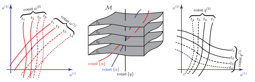
In this appendix we provide mathematical preliminaries that will be useful for the hydrodynamics examples given in Sec. V.2.
In Sec. V.1 we saw an example of a theory which is formulated in a manifestly Lorentz-covariant, four-dimensional fashion. In contrast, the Eulerian and Lagrangian descriptions of the physics of fluids and materials is usually presented in a three-dimensional form, with time being a parameter. However, this hides the geometric, coordinate-independent physics. Instead, we will take a four-dimensional view and treat all quantities as functions, vectors, tensors, and tensor densities on a manifold with a natural time function. For background, see any standard differential geometry text Spivak (1970); Schutz (1980); Wald (1984).
C.1 Euler and Lagrange coordinates
Our geometric setting is a four-dimensional Lorentzian manifold , which we declare to have a natural time function . We only consider coordinate systems which have as one of the four coordinate functions, e.g., . Remember that a coordinate system is a collection of functions. The superscript runs over 0–3 and merely labels the set of four functions; it is not a vector index on these functions. We will use Greek letters to denote spacetime indices that run over 0–3 and Latin letters for spatial indices over 1–3.
To connect with the usual Eulerian and Lagrangian descriptions of continuum mechanics, we will introduce (at least) two coordinate systems below. The Eulerian and Lagrangian descriptions of continuum mechanics both provide useful insight into the evolution of continuum flows. While the Eulerian description of fluids is more popular, it is far easier to construct actions for fluid dynamics without constraints in the Lagrangian description (see e.g., Eckart (1960); Katz (1961); Seliger and Whitham (1968); Morrison (1998)). We will generally adopt the Lagrangian description when describing the actions and performing the variations in Sec. V.2, but also provide the Eulerian form for the equations of motion.
In the more widely used Eulerian description, material flows past the “lab frame” Eulerian coordinates. The Lagrangian formulation instead describes the evolution from the viewpoint of individual fluid elements or parcels tracing out paths in the “lab frame”.
We denote the Eulerian coordinate system by , again with . We will use lower-case Latin indices to label the spatial Eulerian coordinate functions, , and for spatial components of tensors in Eulerian coordinates. Next, consider a fluid or material flowing in this space, and at some initial or fiducial time, label the fluid elements with spatial coordinates . Now promote these labels to functions on the whole manifold so that they are constant on each world-line, or fluid parcel’s trajectory through spacetime (see Fig. 4). That is, each choice of fixed labels the trajectory of an individual fluid parcel through spacetime. Now taking , these four functions are a valid coordinate system. We will use capital Latin indices from the beginning of the alphabet to label the spatial Lagrangian coordinate functions, , and for spatial components of tensors in Lagrangian coordinates. The simplest and most common choice for comes from taking .
C.2 Coordinate transformations
Each coordinate system comes equipped with its own coordinate basis vectors ( and ) and coordinate basis one-forms ( and ). It is with respect to these bases that vector and tensor components are evaluated in these coordinate systems. The spatial bases and are notationally unambiguous, and we will abbreviate them as and , respectively. However, we must pay special attention to .
In an arbitrary coordinate system, the meaning of is “partial derivative in the direction of while holding all other constant.” However, writing lacks the information of which three coordinates are being held constant, since the coordinate function is common to all coordinate systems. Therefore, we introduce the following notation. We define
| (287) |
for any coordinate system , either or (or others, in the case of multifluids). These 4-vectors are the tangents to the world-lines of constant . For convenience we also introduce and .
To see how to transform coordinate components of tensors between the Lagrangian and Eulerian coordinate system (and importantly, how to relate to ), we must introduce the Jacobian matrix between the two coordinate systems. The Jacobian matrix is given by
| (288) |
where we have defined (labeled with the two coordinate systems) as the purely spatial “vector” which is the part of the relative velocity of the coordinates, as measured by an observer at constant , with components . We have also defined the purely spatial Jacobian matrix (also labeled with the two coordinate systems). From the form of the full Jacobian matrix we can easily see that purely spatial vectors (ones which are tangent to surfaces of const) may be transformed between coordinate systems with just the matrix. We write the components of as
| (289) |
which is sometimes called the deformation gradient in continuum mechanics.131313The symbol is sometimes used to denote an orthonormal frame field, but for our usage, it is literally just a Jacobian matrix. This Jacobian transforms purely spatial vectors from the Lagrangian coordinate basis to the Eulerian one, and the spatial components of one-forms in the opposite sense:
| (290) |
A special case of this is the spatial gradient of a scalar function,
| (291) |
The determinant of the spatial Jacobian matrix is sometimes also called the Jacobian, and it is given by
| (292) |
It is also the determinant of the full Jacobian matrix.
When it exists, it is straightforward to see that the inverse matrix, has the same block form as (288), but exchanging . It is also easy to verify that
| (293) |
We write the components of as
| (294) |
Since is generally not symmetric, neither is its inverse. Naturally the determinant of the inverse is the multiplicative inverse of , i.e. . The relative velocity identities of (293) in components read
| (295) |
With the inverse Jacobian matrix, we have two more transformation rules to add to (290):
| (296) |
Using Cramer’s rule it is typical to write the inverse matrix in terms of the transposed matrix of cofactors,
| (297) |
where the cofactor matrix is defined to be
| (298) |
From the definition of an inverse matrix, we immediately get two identities involving the cofactor matrix : one via the left inverse and one via the right inverse. These two identities are
| (299) |
and
| (300) |
We find a third identity from the symmetry of partial derivatives. Notice in the definition (298) that both derivative indices are contracted with the completely anti-symmetric Levi-Civita tensor, which has the free upper index . Taking the divergence on that free index gives
| (301) |
This establishes that is divergence-free on its second (upper) index,
| (302) |
This result only holds for the second index, since in general the cofactor matrix is not symmetric.
With the conventional choice of coordinates [], the volume of the fluid element at initial time is , while at a later time its volume is . The Jacobian thus accounts for the volume changes that result from dynamical evolution. Mass conservation then requires the density of a fluid element to be related to its initial density by the ratio of the volume elements at the two times,
| (303) |
where the mass element is . A quantity which acquires factors of Jacobian determinants when changing coordinate systems is called a density (e.g., scalar density or tensor density). Specifically, a tensor density of weight transforms from coordinate system to coordinate system as
| (304) | ||||
| (305) |
since from (292). A simple way to turn a tensor into a tensor density is to multiply it by a factor of . Thus we say that is a scalar density of weight . We adopt the overbar on some tensors to indicate tensor densities of non-zero weight , which have gained a factor of when transformed to the Eulerian coordinates.
C.3 Metric and derivatives
In order to measure the lengths of spatial vectors, we must introduce a spatial metric . In Eulerian coordinates, it has components in , with inverse metric such that . The metric and inverse are used to “raise” and “lower” contravariant and covariant tensor indices. When expressed in Lagrangian coordinates, it is traditionally represented as and called the Cauchy-Green deformation tensor Oswald (2009)
| (306) |
or, in terms of the Jacobian matrix and its inverse, the deformation tensor and its inverse are
| (307) |
With the conventional choice of coordinates [], at time , the spatial Jacobian matrix is instantaneously equal to the identity, , so we instantaneously have . The metric determinant in different coordinate systems are related through the Jacobian:
| (308) |
where and .
We now turn to how -components of vectors are related in the Eulerian and Lagrangian coordinates. Using the full Jacobian, we have
| (309) |
which would be written in the more traditional fluid mechanics literature as
| (310) |
where we have defined the “vector” . In fact, the combination is a true tangent vector so we define the symbol
| (311) |
and with Eulerian coordinate components . This vector is easily seen to be purely spatial, since , and so is tangent to surfaces of const.141414The notation means the action of vector on the scalar , i.e. to take a directional derivative of on the manifold in the direction of .
Equation 310 [or (311)] relates three tangent vectors, and therefore holds as an identity when acting on scalar functions. This is the usual “material derivative” but only when the vector acts on a manifold scalar function. If we want to take derivatives of tensors on this manifold, then we will have to use the covariant “parameter derivative” along these tangent vector fields. When acting on a scalar field, the parameter derivative along curves of constant agrees with the material derivative. In general, to evaluate the parameter derivative we need a covariant derivative (or connection), , and the parameter derivative is given by
| (312) |
where is the 4-vector which is tangent to the curve with parameter , with components where the world-line coordinates are . When acting on a scalar, any covariant derivative agrees with the usual partial derivative, . When acting on vectors and one-forms, we need the non-tensorial connection coefficients to relate the covariant and partial derivatives:
| (313) | ||||
| (314) |
For a tensor density of weight , we also need to add the single correction term,
| (315) |
In this work, we fix the spatial part of the connection coefficients by demanding that the covariant derivative is compatible with the spatial metric, , so that . This means that our connection coefficients are the usual Christoffel coefficients when the indices are all spatial Wald (1984). In Eulerian coordinates, the Christoffel coefficients of are151515We use an overbar to match the notation for covariant ) and partial in Eulerian coordinates and should not be taken to imply that the connection coefficients are tensor densities.
| (316) |
while in Lagrangian coordinates, they are
| (317) |
For example, if we are working in Cartesian coordinates and , then .
There is still freedom to fix time components of .161616Thiffeault noted Thiffeault (2001) that other covariant time derivatives, , can be defined by using a non-tensorial rank-2 quantity . In our 4-dimensional language, we see that the 3-dimensional quantity is simply the choice of components of . Thiffeault separates out an arbitrary tensorial part which may be freely specified, and modifies the derivative presented here through (318) with correction terms for contravariant indices and correction terms for covariant indices. For example, in Lagrangian coordinates, choosing (the rate-of-strain tensor, defined below) yields the Jaumann corotational derivative. Consider for example the acceleration vector of the world lines of constant ,
| (319) | ||||
| (320) | ||||
| (321) |
where we are parametrizing the world-line by the parameter , so the tangent vector has (in both Eulerian and Lagrangian coordinates). If we choose to set ,171717If we formulate the theory in 4 dimensions with a 4-metric that satisfies , , and =0, then the choice in the coordinates is consistent with metric-compatibility with the 4-metric. then this acceleration vector agrees with the usual notion in the fluid mechanics literature: that the acceleration vector is the “material derivative” of the velocity vector,
| (322) | ||||
| or, in Cartesian coordinates with a flat spatial metric, | ||||
| (323) | ||||
Often times we will want to be able to express time derivatives of components of tensors in both the Eulerian and Lagrangian coordinates. For example, we might ask: what is the relation between
| and | (324) |
This is most easily answered with the Lie derivative along some vector field . The Lie derivative satisfies
| (325) |
where and are constants. In some arbitrary coordinate system, the components of the Lie derivative of some tensor along a vector field is
| (326) | ||||
where there is a correction term for each contravariant index, a correction term for each covariant index, and is the weight of the tensor density.
The Lie derivative is easy to evaluate when in a coordinate system where is a coordinate basis vector: the components will be constant [e.g., ] and so all the “correction” terms will vanish. This is convenient when taking the Lie derivative along or , which are easiest to evaluate in their respective coordinate systems. Specifically,
| (327) | ||||
| (328) |
Using the above properties we can relate partial derivatives along to those along . Using from (311), we have from (325)
| (329) |
which is true as an operator equation acting on any type of tensor. The LHS is best evaluated in the coordinate system, while the first term on the RHS is best evaluated in the coordinate system. This expression can be used to give the so-called “convective derivative” relating time derivatives in different coordinate systems. Taking components gives, for example,
| (330) | ||||
| (331) | ||||
Another useful example which we will often encounter is the Lie derivative of a scalar density of weight , such as the mass density , entropy density, , or energy density . We evaluate (329) on , evaluating the LHS in the coordinates and the RHS in the coordinates (then transforming the resulting scalar density back to coordinates by multiplying by ):
| (332) | ||||
| (333) |
It is easy to show that so that (333) can be written as
| (334) |
C.4 Physical quantities
Now we may define some of the physical quantities necessary to describe fluids. We have already seen the spatial velocity of a fluid element of constant , as measured in coordinates, is , which are tangent to the fluid worldlines of constant . They are evaluated in coordinates via the parameter derivative of the coordinate functions. Since the coordinates are just scalars, the parameter derivatives agree with partial derivatives:
| (335) |
Also mentioned above, the spatial acceleration vector comes from the covariant parameter derivative along the world-lines, . Further, we will continue to use a covariant derivative which is metric-compatible with the spatial metric, , and fix (some) time components of the -coordinate connection via , so that the acceleration is given in components by
| (336) |
In flat space and Cartesian coordinates, this coincides with the “material derivative” of velocity,
| (337) |
A useful form of the acceleration which we often encounter is given by
| (338) | ||||
| (339) | ||||
| (340) |
It is traditional to define the relative strain tensor , which is (half) the difference between the metric at any time and a reference tensor
| (341) |
The reference tensor is symmetric and constant in the Lagrange coordinates. For viscous fluids it can be arbitrarily defined to be match the metric at some particular time . For an elastic material it is useful to set to be the ‘background’ material deformation for which the elastic stress is zero.
Another quantity we will encounter in the equations of motion is the rate of change of the metric (or Cauchy-Green deformation tensor) along the fluid world-lines. This is known as the rate of strain tensor,
| (342) | ||||
| (343) |
For component calculations, it is useful to expand via (307), , giving
| (344) |
We can also express the rate of strain tensor in Eulerian coordinates, by using the Lie derivative identity in (329). This gives
| (345) | ||||
| (346) |
The term arising from vanishes since we are considering stationary metrics. The astute reader will note that (346) is valid even for curved metrics and curvilinear coordinates, since throughout (342-346) we have only used a Lie derivative identity and the stationarity of the metric in coordinates.
Appendix D Deriving Euler’s equation in coordinate covariant form
In this appendix, we give some details of the calculation for deriving the Euler-Lagrange equations for an adiabatic and inviscid (i.e., perfect) fluid. We do this to help fill in the gaps not provided in Sec. V.2.1.
The Lagrangian density for a perfect fluid is given in (160) and the Euler-Lagrange equations of motion in (127). With we have that
| (347) |
upon recalling from (289) that . Computing each term above in turn yields
| (348) |
and
| (349) | ||||
| (350) |
upon using the identity in (302). The term has two contributions that are vital for ensuring that the fluid equations of motion are covariantly represented in any coordinate system. The first comes from the fact that the space-time metric is evaluated on the coordinates of the fluid element’s trajectory. The second comes from the fact that is generally non-zero in curved spaces and/or in curvilinear coordinates, such as the Lagrangian coordinates . Therefore,
| (351) |
It is straightforward to show using the definition of the Christoffel connection coefficients [given in (316)] that the first term in (351) can be written as
| (352) |
Likewise, using (292), Jacobi’s formula, and (317) one can show that
| (353) |
Then, the second term in (351) is
| (354) |
Combining these results all together gives for the Euler-Lagrange equations the following expression
Written in this way we see that the first line is proportional to the covariant parameter derivative of from (340), and that the second line is proportional to the covariant spatial derivative of the pressure,
| (355) |
In general curvilinear coordinates and a possibly curved space we thus find
| (356) |
Since only covariant derivatives that are compatible with the metric appear in this expression we can freely raise the spatial index “” by contracting both sides with the metric to give,
| (357) |
If one is working in rectangular coordinates in a flat space then the first term in (351) for vanishes while the second one generally remains except for steady flows.
Appendix E The classical limit of nonequilibrium quantum theory
In this appendix, we show how the nonconservative action in (9) can be derived from the classical limit of quantum mechanical systems in nonequilibrium (see e.g., Calzetta and Hu (2008); Weiss (1999)). This result provides a fundamental justification for the manipulations and assumptions we have made in extending classical Lagrangian and Hamiltonian mechanics and field theories to nonconservative systems and dissipative problems. For presentation purposes, we focus on discrete quantum mechanical systems but the steps are similar for nonequilibrium quantum field theories.
Consider a closed (i.e., unitary) quantum system with accessible degrees of freedom and variables that we will eliminate. The action is
| (358) |
where the last term accounts for mutual interactions.
The density matrix at the initial time is given by . At some arbitrary future final time the density matrix will have unitarily evolved to via the time-evolution operator so that
| (359) |
which has matrix elements given by
| (360) |
The reduced density matrix for is defined as the trace taken over states at the final time of (360),
| (361) |
The reduced density matrix is the quantity that one computes expectation values of an operator through tracing over in the usual manner, . Assuming that the initial states are complete it follows that we can put two insertions of the identity operator,
| (362) |
into (361) which yields
| (363) |
upon using (359) to express in terms of . The matrix element in the second line has a well known path integral representation in terms of the classical (conservative) action in (358),
Assuming for simplicity that the initial states are factorized, so that
| (364) |
we find that the reduced density matrix can be written as
| (365) |
where is called the influence action and determines the influence on the accessible variables of all the contributions from the integrated out quantum degrees of freedom Feynman and Vernon (1963),
| (366) | ||||
Notice that the insertion of two identity operators into the reduced density matrix and their corresponding path integral representations leads quite naturally to the appearance of a doubled set of degrees of freedom for the whole problem. That this happens is a result of the density matrix at the final time being evolved by two unitary operators in (359) that, in turn, is due to the structure of evolving a system from some initial state in a causal manner. This formulation of quantum theory is sometimes referred to as the “in-in” formalism Schwinger (1961); Keldysh (1964); Jordan (1986); Calzetta and Hu (1987) because one keeps track of how operators of nonequilibrium quantum systems evolve from the “in” state to the “in” state (i.e., expectation values) as opposed to the “out” state (i.e., matrix elements and amplitudes).
In many systems where the path integrals can be computed, contains an imaginary part,
| (367) |
that drives the accessible variables to decohere towards classicality. For example, if we take the to be harmonic oscillators coupled linearly to ,
| (368) |
then it follows that Calzetta et al. (2003); Calzetta and Hu (2008)
| (369) |
where the expectation value is taken in the (zero-mean, Gaussian) initial state of the . Here, is the quantum version of the “” variable that appears in the nonconservative classical mechanics formulation of Secs. II and IV. For a large class of initial states, the imaginary part of the influence action is positive so that the norm of (367) decays super exponentially when increases thereby suppressing quantum fluctuations and inciting decoherence. As a result, the phase in the path integrand of (365) becomes peaked around configurations where is small, which causes the reduced density matrix to be (nearly) diagonal (see e.g., Feynman and Vernon (1963); Calzetta et al. (2003); Calzetta and Hu (2008)).
We can now take the limit of the reduced density matrix in (365) to find — using the stationary phase approximation — that the dominant contribution to the reduced density matrix comes from181818 The corrections come from quantum fluctuations that manifest as classical stochastic forces coupled to through . Following Feynman and Vernon (1963); Calzetta et al. (2003), for the oscillator example in (368) and (369), the statistical two-point correlations, , imply that .
| (370) |
When written out in terms of Lagrangians we find a familiar expression, namely (9),
where the real part of the influence action is the time integral of the nonconservative potential . Therefore, the classical limit of the quantum theory in non-equilibrium is described by exactly the nonconservative action written down in Galley (2013) and (9). Of course, in cases where cannot be computed explicitly there still exists a formal expression for it given in (366) and thus a relationship with . The result of this appendix can also be found by using the more abstract “in-in” generating functional language to derive the nonconservative action from the coarse-grained effective action (see e.g., Calzetta and Hu (2008)) via a loop expansion in powers of .
This appendix has established that nonconservative classical mechanics is derivable from a more complete fundamental quantum theory, provide there is sufficient decoherence that a classical limit can be reached. See also recent work in Kuwahara et al. (2013) who quantize the nonconservative Hamiltonian of Galley (2013) and find a relation with Thermo Field Dynamics. In addition, see work in Polonyi (2014) for further connections between and the “in-in” formulation of non-equilibrium quantum field theories.
References
- Hamilton (1834) W. R. Hamilton, Phil. Trans. Roy. Soc. Lon , 95 (1834).
- Goldstein et al. (2002) H. Goldstein, C. Poole, and J. Safko, Classical mechanics, 3rd ed. (Addison-Wesley, 2002).
- Noether (1918) E. Noether, Nachr. D. Koenig. Gesellsch. D. Wiss. Zu Goettingen, Math-phys. Klasse 1918: p. 235-237 , 235 (1918).
- Dirac (1950) P. A. M. Dirac, Can. J. Math 2, 129 (1950).
- Calzetta and Hu (2008) E. A. Calzetta and B.-L. B. Hu, Nonequilibrium Quantum Field Theory (Cambridge University Press, 2008).
- DeGroot and Mazur (1984) S. DeGroot and P. Mazur, Non-equilibrium Thermodynamics, Dover Books on Physics Series (Dover Publications, 1984).
- Rayleigh (1896) J. W. S. B. Rayleigh, The theory of sound, Vol. 2 (Macmillan, 1896).
- Virga (2014) E. G. Virga, ArXiv e-prints (2014), arXiv:1406.6906 [math-ph] .
- Bauer (1931) P. S. Bauer, Proceedings of the National Academy of Sciences of the United States of America 17, 311 (1931).
- Bateman (1931) H. Bateman, Physical Review 38, 815 (1931).
- Dreisigmeyer and Young (2003) D. W. Dreisigmeyer and P. M. Young, Journal of Physics A: Mathematical and General 36, 8297 (2003).
- Staruszkiewicz (1970) A. Staruszkiewicz, Annalen der Physik 480, 362 (1970).
- Jaranowski and Schäfer (1997) P. Jaranowski and G. Schäfer, Phys. Rev. D 55, 4712 (1997).
- Galley (2013) C. R. Galley, Phys. Rev. Lett. 110, 174301 (2013), arXiv:1210.2745 [gr-qc] .
- Machta et al. (2013) B. B. Machta, R. Chachra, M. K. Transtrum, and J. P. Sethna, Science 342, 604 (2013).
- Burgess (2007) C. P. Burgess, Ann. Rev. Nucl. Part. Sci. 57, 329 (2007), hep-th/0701053 .
- Manohar (1997) A. V. Manohar, Lect.Notes Phys. 479, 311 (1997), arXiv:hep-ph/9606222 [hep-ph] .
- Rothstein (2002) I. Z. Rothstein, in Prepared for Theoretical Advanced Study Institute in Elementary Particle Physics (TASI 2002): Particle Physics and Cosmology: The Quest for Physics Beyond the Standard Model(s), Boulder, Colorado (2002) hep-ph/0308266 .
- Goldberger (2007) W. Goldberger, in Paricle Physics and Cosmology: The Fabric of Spacetime, Volume LXXXVI: Lecture notes of the Les Houches Summer School, edited by F. Bernardeau, C. Grojean, and J. Dalibard (Elsevier Science, 2007) hep-ph/0701129 .
- (20) C. R. Galley, D. Tsang, and L. C. Stein, (in preparation).
- Wheeler and Feynman (1949) J. A. Wheeler and R. P. Feynman, Rev. Mod. Phys. 21, 425 (1949).
- Weiss (1999) U. Weiss, Quantum Dissipative Systems, 2nd ed. (World Scientific, 1999).
- Scheck (1996) F. Scheck, Mechanics: From Newton’s Laws to Deterministic Chaos, 3rd ed. (Springer, Berlin, 1996).
- Goldberger and Rothstein (2006) W. D. Goldberger and I. Z. Rothstein, Phys. Rev. D73, 104030 (2006), arXiv:hep-th/0511133 [hep-th] .
- Galley et al. (2010) C. R. Galley, A. K. Leibovich, and I. Z. Rothstein, Phys. Rev. Lett. 105, 094802 (2010), arXiv:1005.2617 [gr-qc] .
- Jackson (1999) J. D. Jackson, Classical electrodynamics, 3rd ed. (Wiley, New York, NY, 1999).
- Landau and Lifshitz (1986a) L. Landau and E. Lifshitz, Classical Theory of Fields, Course of Theoretical Physics (Butterworth-Heinemann, 1986).
- Koga (2004) J. Koga, Phys. Rev. E 70, 046502 (2004).
- Ober-Blöbaum et al. (2013) S. Ober-Blöbaum, M. Tao, M. Cheng, H. Owhadi, and J. E. Marsden, Journal of Computational Physics 242, 498 (2013), arXiv:1103.1859 [math.NA] .
- Misner et al. (1973) C. W. Misner, K. S. Thorne, and J. A. Wheeler, Gravitation (Freeman, San Francisco, 1973).
- Soper (2008) D. E. Soper, Classical Field Theory (Dover Publications, New York, 2008).
- Galley and Leibovich (2012) C. R. Galley and A. K. Leibovich, Phys. Rev. D86, 044029 (2012), arXiv:1205.3842 [gr-qc] .
- Kevrekidis (2014) P. G. Kevrekidis, Phys. Rev. A 89, 010102 (2014).
- Dauxois and Peyrard (2006) T. Dauxois and M. Peyrard, Physics of solitons (Cambridge University Press, 2006).
- Malomed (2002) B. A. Malomed, Progress in Optics 43, 71 (2002).
- Malomed (2006) B. A. Malomed, Soliton management in periodic systems (Springer, 2006).
- Andersson and Comer (2013) N. Andersson and G. L. Comer, ArXiv e-prints (2013), arXiv:1306.3345 [gr-qc] .
- Prix (2004) R. Prix, Phys. Rev. D69, 043001 (2004), arXiv:physics/0209024 [physics] .
- Endlich et al. (2013) S. Endlich, A. Nicolis, R. A. Porto, and J. Wang, Phys. Rev. D88, 105001 (2013), arXiv:1211.6461 [hep-th] .
- Grozdanov and Polonyi (2013) S. Grozdanov and J. Polonyi, (2013), arXiv:1305.3670 [hep-th] .
- Ray (1972) J. R. Ray, J. Math. Phys. 13, 1451 (1972).
- Eckart (1960) C. Eckart, Physics of Fluids 3, 421 (1960).
- Katz (1961) S. Katz, Physics of Fluids 4, 345 (1961).
- Seliger and Whitham (1968) R. L. Seliger and G. B. Whitham, Royal Society of London Proceedings Series A 305, 1 (1968).
- Morrison (1998) P. Morrison, Rev. Mod. Phys. 70, 467 (1998).
- Landau and Lifshitz (1986b) L. Landau and E. Lifshitz, Fluid Mechanics, Course of Theoretical Physics (Butterworth-Heinemann, 1986).
- Batchelor (1967) G. K. Batchelor, An Introduction to Fluid Dynamics (Cambridge University Press, Cambridge, 1967).
- Andersson and Comer (2010) N. Andersson and G. L. Comer, Royal Society of London Proceedings Series A 466, 1373 (2010), arXiv:0908.1707 [physics.flu-dyn] .
- Kim and Karrila (1991) S. Kim and S. J. Karrila, Microhydrodynamics (Butterworth-Heinemann New York:, 1991).
- Landau and Lifshitz (1986c) L. Landau and E. Lifshitz, Theory of Elasticity, Course of Theoretical Physics (Butterworth-Heinemann, 1986).
- Oswald (2009) P. Oswald, Rheophysics (Cambridge University Press, Cambridge, UK, 2009).
- Keramidas Charidakos et al. (2014) I. Keramidas Charidakos, M. Lingam, P. J. Morrison, R. L. White, and A. Wurm, ArXiv e-prints (2014), arXiv:1407.3884 [physics.plasm-ph] .
- (53) D. Tsang, C. R. Galley, L. C. Stein, and K. N. Gourgouliatos, (in prepartion).
- Onsager and Machlup (1953) L. Onsager and S. Machlup, Phys. Rev. 91, 1505 (1953).
- Landau and Lifshitz (1957) L. Landau and E. Lifshitz, JETP 32, 618 (1957), [Sov. Phys. JETP 5, 512 (1957)].
- Martin et al. (1973) P. Martin, E. Siggia, and H. Rose, Phys. Rev. A8, 423 (1973).
- De Dominicis and Peliti (1978) C. De Dominicis and L. Peliti, Phys. Rev. B18, 353 (1978).
- Eyink (1996) G. L. Eyink, Phys. Rev. E54, 3419 (1996).
- Eyink (1998) G. L. Eyink, Progress of Theoretical Physics Supplement 130, 77 (1998).
- Kovtun et al. (2014) P. Kovtun, G. D. Moore, and P. Romatschke, JHEP 1407, 123 (2014), arXiv:1405.3967 [hep-ph] .
- Israel and Stewart (1979) W. Israel and J. M. Stewart, Annals of Physics 118, 341 (1979).
- Spivak (1970) M. Spivak, A comprehensive introduction to differential geometry, A Comprehensive Introduction to Differential Geometry No. v. 1 (Brandeis University, 1970).
- Schutz (1980) B. Schutz, Geometrical Methods of Mathematical Physics (Cambridge University Press, 1980).
- Wald (1984) R. Wald, General Relativity (University of Chicago Press, 1984).
- Thiffeault (2001) J.-L. Thiffeault, Journal of Physics A Mathematical General 34, 5875 (2001), nlin/0102038 .
- Oldroyd (1950) J. G. Oldroyd, Royal Society of London Proceedings Series A 200, 523 (1950).
- Feynman and Vernon (1963) R. Feynman and F. Vernon, Ann. Phys. 24, 118 (1963).
- Schwinger (1961) J. Schwinger, J. Math. Phys. 2, 407 (1961).
- Keldysh (1964) L. V. Keldysh, Zh. Eksp. Teor. Fiz. 47, 1515 (1964), [English translation, Sov. Phys. JEPT 20, 1018 (1965)].
- Jordan (1986) R. D. Jordan, Phys. Rev. D33, 444 (1986).
- Calzetta and Hu (1987) E. Calzetta and B. L. Hu, Phys. Rev. D35, 495 (1987).
- Calzetta et al. (2003) E. Calzetta, A. Roura, and E. Verdaguer, Physica A (Amsterdam) 319, 188 (2003).
- Kuwahara et al. (2013) Y. Kuwahara, Y. Nakamura, and Y. Yamanaka, Physics Letters A 377, 3102 (2013).
- Polonyi (2014) J. Polonyi, (2014), arXiv:1407.6526 [hep-th] .