Resonances in ultracold dipolar atomic and molecular gases

Abstract

A previously developed approach for the numerical treatment of two particles that are confined in a finite optical-lattice potential and interact via an arbitrary isotropic interaction potential has been extended to incorporate an additional anisotropic dipole-dipole interaction. The interplay of a model but realistic short-range Born-Oppenheimer potential and the dipole-dipole interaction for two confined particles is investigated. A variation of the strength of the dipole-dipole interaction leads to diverse resonance phenomena. In a harmonic confinement potential some resonances show similarities to $s$-wave scattering resonances while in an anharmonic trapping potential like the one of an optical lattice inelastic confinement-induced dipolar resonances occur. The latter are due to a coupling of the relative and center-of-mass motion caused by the anharmonicity of the external confinement.

• March 14, 2024

1 Introduction

In recent years significant experimental progress has lead to sophisticated cooling and trapping techniques of polar molecules and of atomic species having a large dipole moment [1, 2, 3, 4]. A very promising approach for achieving ultracold polar molecules is the formation of weakly-bound molecules making use of a magnetic Feshbach resonance and a subsequent transfer to the ground state using the STIRAP (stimulated Raman adiabatic passage) scheme [5]. Based on this method gases of motionally ultracold RbK [6] or LiCs [7] molecules in their rovibrational ground states were achieved. This fascinating progress paved the way towards degenerate quantum gases with predominant dipole-dipole interactions (DDI). In the case of magnetic dipoles the Bose-Einstein condensation (BEC) of ${}^{52}\text{Cr}$, an atom with a large magnetic moment of 6 $\mu_{B}$, was already achieved in 2004 [8]. Although in chromium the DDI can be enhanced relative to the atomic short-range interaction by decreasing the strength of the latter using a Feshbach resonance [9], the DDI is typically still smaller or at most of the same magnitude as the van-der-Waals forces. In order to create an atomic gas with a DDI larger than the van-der-Waals forces, it was possible to realise a BEC of Dysprosium ($10\mu_{B}$) [10] and Erbium ($12\mu_{B}$) [11].

The properties of the DDI are completely different from those of isotropic short-range interactions, e. g., the ones between two atoms with no DDI. The DDI has a long-range character as it decays as $1/r^{3}$, where $r$ is the inter-particle distance, and it is anisotropic which means that even the sign of the interaction depends on the angle $\theta$ between the polarisation direction and the relative position of the particles.

A full and quantitative understanding of the behaviour of two particles in an external trapping potential is a prerequisite for the manipulation and control of ultracold two-body systems that have been proposed for possible quantum-computer realisations [12, 13]. This knowledge about the microscopic two-body physics is also important for the understanding of the rich physics of the corresponding many-body systems. For example, more accurate Bose-Hubbard parameters for describing an ultracold quantum gas in an optical lattice have been extracted from two-particle calculations in the absence [14] or the presence of DDI [15]. Furthermore, inelastic confinement-induced two-body resonances [16, 17] were found to have caused massive atom losses also in quantum gases with many particles [18]. Evidently, the possibility to vary the interaction strength within ultracold atomic quantum gases with the aid of two-body magnetic Feshbach resonances has been of paramount importance for the whole research field.

Different theoretical approaches to describe dipolar systems have been reported earlier. To describe an ultracold dipolar gas trapped in a harmonic confinement, in [19, 20] a pseudo potential as a function of the dipole moment is proposed for the short-range interaction, while for the long-range potential the anisotropic DDI is adopted. The approach described in [21] uses a hard-sphere potential for the short-range part of the interaction potential between two dipolar particles in free space. In these approaches $s$-wave like scattering resonances induced by the dipolar interactions were observed. Following the prediction of elastic confinement-induced resonances in quasi-1D confinement [22, 23], such resonances for dipolar systems were considered in [24, 25].

The approach described in the present work extends the method described in [26] which allows for the use of a realistic, numerically given Born-Oppenheimer potential curve for the short-range part of the interaction potential by adding an additional DDI. In contrast to the use of a $\delta$ pseudo-potential that supports a single bound state, the use of a realistic short-range potential supports often many deeply bound states. Furthermore, in contrast to numerous previous works, see e. g. [27, 28, 24, 29], in our approach the external trap potential is chosen as a finite optical-lattice potential, i. e., a truncated Taylor series for a $\sin^{2}$ or $\cos^{2}$ optical-lattice potential. While a truncation at the second order yields a harmonic trapping potential, anharmonic multi-well potentials can be achieved, if the truncation is performed at higher orders. In this work it will be demonstrated that in an anharmonic trapping potential the coupling of center-of-mass and relative motion leads to the occurrence of inelastic resonances at which bound states with some center-of-mass excitation couple to states of unbound dipoles. This mechanism is analogous to the inelastic confinement-induced resonances described in [16, 30, 17] for ultracold atomic systems without DDI.

This article is organised as follows. First, the Hamiltonian and the numerical method are introduced in Section 2 and Section 3, respectively. In Section 4 the influence of the dipolar interaction is investigated for two different trapping potentials. The results for an isotropic harmonic trap are shown in Section 4.1, the ones for an anisotropic sextic potential with coupling between center-of-mass and relative motions in Section 4.2. A conclusion is provided in Section 5.

2 Two-Body Problem of Trapped Dipolar Particles

A system of two dipolar particles with masses $m_{1}$, $m_{2}$ and the absolute coordinates $\mathbb{r_{1}}$, $\mathbb{r_{2}}$ trapped in an optical lattice is described by the Hamiltonian

$$\begin{split}\hat{\rm H}=\hat{\rm T}_{1}(\mathbb{r_{1}})+\hat{\rm T}_{2}(\mathbb{r_{2}})+\hat{\rm V}_{1}(\mathbb{r_{1}})+\hat{\rm V}_{2}(\mathbb{r_{2}})+\hat{\rm V}_{\rm int}(\mathbb{r_{1}}-\mathbb{r_{2}})\;,\end{split}$$ (1)

where $\hat{\rm T}_{i}(\mathbb{r_{i}})$ is the kinetic energy operator $\frac{\hat{\mathbb{p}}_{i}^{2}}{2m_{i}}$ for each particle. The trapping potential is chosen as a $\sin^{2}$ optical lattice

$$\begin{split}V_{i}(\mathbb{r_{i}})=\sum_{j=x_{i},y_{i},z_{i}}V_{0,j}\sin^{2}(k_{j}j)\end{split}$$ (2)

which can be experimentally obtained by the superposition of counter-propagating laser beams [31], where the parameters $V_{0,j}$ and $k_{j}$ are the potential depth and the components of the wavevector $k_{j}=2\pi/\lambda_{j}$, respectively.

Relative (rm) and center-of-mass (CM) motion coordinates $\mathbb{r}=\mathbb{r_{1}}-\mathbb{r_{2}}$, $\mathbb{R}=\mu_{1}\mathbb{r_{1}}+\mu_{2}\mathbb{r_{2}}$, respectively, are introduced to transform the two-body Hamiltonian in Eq. (1) into

$$\begin{split}\hat{\rm H}(\mathbb{r},\mathbb{R})=\hat{\rm h}_{\rm rm}(\mathbb{r})+\hat{\rm h}_{\rm CM}(\mathbb{R})+\hat{\rm W}(\mathbb{r},\mathbb{R})\end{split}$$ (3)

where $\hat{\rm h}_{\rm rm}$ and $\hat{\rm h}_{\rm CM}$ are the separable parts of the Hamiltonian in relative and center-of-mass coordinates, respectively, and $\mu_{i}=\frac{m_{i}}{m_{1}+m_{2}}$. The coupling term $\hat{\rm W}(\mathbb{r},\mathbb{R})$ describes the non-separable parts of the Hamiltonian that originate from the non-separability of the optical-lattice potential in relative and center-of-mass coordinates. The center-of-mass motion part

$$\begin{split}\hat{\rm h}_{\rm CM}(\mathbb{R})=\frac{\hat{\mathbb{P}}^{2}}{2M}+V_{\rm CM}(\mathbb{R})\end{split}$$ (4)

of the Hamiltonian in Eq. (3) and the relative-motion part

$$\begin{split}\hat{\rm h}_{\rm rm}(\mathbb{r})=\frac{\hat{\mathbb{p}}^{2}}{2\mu}+V_{\rm rm}(\mathbb{r})+V_{\rm int}(\mathbb{r})\;,\end{split}$$ (5)

contain the respective momentum operators $\hat{\mathbb{p}}$ and $\hat{\mathbb{P}}$ in relative and center-of-mass coordinates, i. e. $\hat{\mathbb{p}}=\hat{\mathbb{p_{1}}}-\hat{\mathbb{p_{2}}}$ and $\hat{\mathbb{P}}=\mu_{1}\hat{\mathbb{p_{1}}}+\mu_{2}\hat{\mathbb{p_{2}}}$. While the implementation of the algorithm also allows for distinguishable particles, in the present work only the special case of identical particles is considered which is in accordance with many experiments [1, 2, 11, 10]. In this case, the separable parts of the optical-lattice potential,

$$\begin{split}V_{\rm CM}(\mathbb{R})=2\sum_{c=x,y,z}V_{0,c}\sin^{2}\left(k_{c}R_{c}\right)\end{split}$$ (6)

and

$$\begin{split}V_{\rm rm}(\mathbb{r})=2\sum_{c=x,y,z}V_{0,c}\sin^{2}\left(\frac{k_{c}r_{c}}{2}\right)\;,\end{split}$$ (7)

and the coupling part

$$\begin{split}\hat{\rm W}(\mathbb{r},\mathbb{R})=-4\sum_{c=x,y,z}V_{0,c}\sin^{2}\left(k_{c}R_{c}\right)\sin^{2}\left(\frac{k_{c}r_{c}}{2}\right)\end{split}$$ (8)

keep a simple form containing the $\sin^{2}$ terms.

The interaction potential $V_{\rm int}(\mathbb{r})=V_{\rm int}(r,\theta)$ in Eq. (5) describes the interaction of two dipolar particles. In the present approach, the interaction potential consists of an isotropic short-range part $V_{\rm sh}$ and of the long-range DDI $V_{\rm dd}$ for aligned dipoles along the $z$ axis,

$$\begin{split}V_{\rm int}(r,\theta)=V_{\rm sh}(r)+V_{\rm dd}(r,\theta)=V_{\rm sh}(r)+\frac{C_{\rm dd}}{4\pi}\frac{1-3\cos^{2}(\theta)}{r^{3}}=V_{\rm sh}(r)-\sqrt{\frac{16\pi}{5}}\frac{C_{\rm dd}}{4\pi}\frac{Y_{2}^{0}(\theta)}{r^{3}}\;,\end{split}$$ (9)

where $C_{\rm dd}=d_{1}d_{2}/\epsilon_{0}$ ($C_{\rm dd}=\mu_{0}\tilde{\mu}_{1}\tilde{\mu}_{2}$) is the coupling constant for the electric dipole moments $d_{1}$ and $d_{2}$ (magnetic dipole moments $\tilde{\mu}_{1}$ and $\tilde{\mu}_{2}$) where $\epsilon_{0}$ is the vacuum permittivity ($\mu_{0}$ the vacuum permeability). Furthermore, in Eq. (9) the spherical harmonic $Y_{2}^{0}(\theta)=\sqrt{5/(16\pi)}(3\cos^{2}(\theta)-1)$ is introduced. The alignment of the electric or magnetic dipoles can be obtained with static electric or magnetic fields, respectively. Additionally, as the applied electric field increases, the dipole moment $d$ continuously increases from zero to the full permanent dipole moment in the case of electric dipoles.

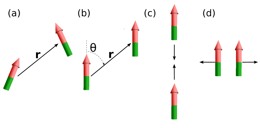
Figure 1: Two particles interacting via a dipole-dipole interaction (DDI): (a) non-polarised case; (b) with polarisation along the $z$ axis; (c) two polarised dipoles in the head-to-tail configuration attracting each other (black arrows); (d) two polarised dipoles in the side-by-side configuration repelling each other (black arrows).

A rather unique feature of the present approach is that the short-range interaction potential $V_{\mathrm{sh}}$ can be chosen arbitrarily as some analytical expression, some numerically given potential curve, or a mixture of both. The only constraint is its isotropy. Choosing a realistic atomic or molecular interaction potential provides the unique opportunity to investigate in a realistic fashion especially the regime where both, the isotropic short-range interaction as well as the DDI, have a comparable influence. Such a study is not possible with model potentials (such as, e. g., zero-range potentials [29] or hard spheres [32]) that do not realistically reproduce the behavior of the tail of the short-range potential.

The anisotropy of the DDI is described by the spherical harmonic $Y_{l=2}^{m=0}(\theta)$, see Eq. (9). The DDI is repulsive for dipoles in the side-by-side configuration and attractive in the head-to-tail configuration, see Fig. 1. Therefore, with increasing dipole moment the overall interaction potential changes dramatically from the generic isotropic short-range interaction to an anisotropic long-range DDI. In addition, the shape of the long-range part of the wavefunction is strongly influenced by the trap and a possible centrifugal barrier.

3 Method

The full treatment of two particles interacting by an arbitrary isotropic interaction potential and confined in a finite optical lattice has been introduced in [26]. In the present work this approach has been extended for treating particles that interact with an additional anisotropic DDI. Details of the original approach with isotropic interactions can be found in [26]. Here, this approach is briefly described and the extension for the inclusion of the DDI is presented.

3.1 Exact Diagonalisation

For a given trapping potential the Schrödinger equation

$$\begin{split}\hat{\rm H}\left|\Psi_{i}\right>=\mathcal{E}_{i}\left|\Psi_{i}\right>\end{split}$$ (10)

of the Hamiltonian of Eq. (3) in relative and center-of-mass coordinates is solved by expanding $\Psi$ in terms of configurations $\Phi$,

$$\begin{split}\Psi_{i}(\mathbb{R},\mathbb{r})=\sum_{k}\mathcal{C}_{ik}\;\Phi_{k}(\mathbb{R},\mathbb{r})\;.\end{split}$$ (11)

The configurations

$$\begin{split}\Phi_{k}(\mathbb{R},\mathbb{r})=\varphi_{i_{k}}(\mathbb{r})\psi_{j_{{}_{k}}}(\mathbb{R})\end{split}$$ (12)

are products of the eigenfunctions $\varphi$ and $\psi$ that are the solutions of the eigenvalue equations

$$\begin{split}\hat{\rm h}_{\rm rm}\left|\varphi_{i}\right>=\epsilon_{i}^{\rm rm}\left|\varphi_{i}\right>,\qquad\hat{\rm h}_{\rm CM}\left|\psi_{j}\right>=\epsilon_{j}^{\rm CM}\left|\psi_{j}\right>\;.\end{split}$$ (13)

of the Hamiltonians for the relative and center-of-mass motions, respectively. Once the eigenvectors $\left|\varphi\right>$ and $\left|\psi\right>$ are obtained from the solution of the corresponding generalised matrix eigenvalue problem with the matrices

$$\begin{split}h_{\mathbb{a},\mathbb{a^{\prime}}}^{\rm rm}=\left<\varphi_{\mathbb{a}}\vphantom{\hat{\rm h}_{\rm rm}\varphi_{\mathbb{a^{\prime}}}}\right|\hat{\rm h}_{\rm rm}\left|\varphi_{\mathbb{a^{\prime}}}\vphantom{\varphi_{\mathbb{a}}\hat{\rm h}_{\rm rm}}\right>,\qquad s_{\mathbb{a},\mathbb{a^{\prime}}}^{\rm rm}=\left<\varphi_{\mathbb{a}}\vphantom{\varphi_{\mathbb{a^{\prime}}}}\right|\left.\varphi_{\mathbb{a^{\prime}}}\vphantom{\varphi_{\mathbb{a}}}\right>\;,\end{split}$$ (14)

$$\begin{split}h_{\mathbb{b},\mathbb{b^{\prime}}}^{\rm CM}=\left<\psi_{\mathbb{b}}\vphantom{\hat{\rm h}_{\rm CM}\psi_{\mathbb{b^{\prime}}}}\right|\hat{\rm h}_{\rm CM}\left|\psi_{\mathbb{b^{\prime}}}\vphantom{\psi_{\mathbb{b}}\hat{\rm h}_{\rm CM}}\right>,\qquad s_{\mathbb{b},\mathbb{b^{\prime}}}^{\rm CM}=\left<\psi_{\mathbb{b}}\vphantom{\psi_{\mathbb{b^{\prime}}}}\right|\left.\psi_{\mathbb{b^{\prime}}}\vphantom{\psi_{\mathbb{b}}}\right>\;\end{split}$$ (15)

with the short hand notation $\mathbb{a}\equiv\alpha,l,m$ and $\mathbb{b}\equiv\beta,L,M$, the ordinary matrix eigenvalue problem

$$\begin{split}\mathbb{H}\mathbb{\mathbf{C}_{i}}=\mathbb{\mathcal{E}_{i}}\mathbb{\mathbf{C}_{i}}\;,\end{split}$$ (16)

for the configurations remains, where the matrix $\mathbb{H}$ is given by

$$\begin{split}H_{k,k^{\prime}}=\left<\Phi_{k}\vphantom{\hat{\rm H}\Phi_{k^{\prime}}}\right|\hat{\rm H}\left|\Phi_{k^{\prime}}\vphantom{\Phi_{k}\hat{\rm H}}\right>\;.\end{split}$$ (17)

In order to extend the approach in [26] to dipolar interactions, matrix elements of the type $\left<\varphi_{\mathbb{a}}\vphantom{V_{\rm dd}\varphi_{\mathbb{a^{\prime}}}}\right|V_{\rm dd}\left|\varphi_{\mathbb{a^{\prime}}}\vphantom{\varphi_{\mathbb{a}}V_{\rm dd}}\right>$ have to be calculated and added to the relative-motion part of the Hamiltonian.

3.2 Basis Set

The numerical method [26] that is extended in this work uses spherical harmonics as basis functions for the angular part of the basis functions. For the radial part of the basis set $B$-spline functions $B_{\alpha}(r)$ of order $k$ are used. The advantage of using $B$ splines is their compactness in space that leads to sparse overlap and Hamiltonian matrices. Another relevant property is the continuity of their derivatives up to order $k-1$.

As a result, the basis functions

$$\begin{split}\phi_{\alpha,l,m}(\mathbb{r})=\frac{B_{\alpha}(r)}{r}Y_{l}^{m}(\theta,\varphi)\;,\end{split}$$ (18)

are used to expand the eigenfunctions

$$\begin{split}\varphi_{i}=\sum_{\alpha=1}^{N_{r}}\sum_{l=0}^{N_{l}}\sum_{m=-l}^{l}c_{i;\alpha lm}\;\phi_{\alpha,l,m}\end{split}$$ (19)

for the relative motion with the expansion coefficients $c_{i,\alpha lm}$. The basis sets are characterised by the upper limits $N_{l}$ of angular momentum in the spherical-harmonics expansion and the number $N_{r}$ of $B$ splines used in the expansion in Eq. (19). The same type of basis functions as in Eq. (18) is used for solving for the center-of-mass motion functions $\psi$.

The computational effort can be drastically reduced by exploiting symmetry properties. The Hamiltonian of two atoms interacting via the interaction potential $V_{\rm int}$ that are trapped in a $\sin^{2}$-like or $\cos^{2}$-like potential oriented along three orthogonal directions is invariant under the symmetry operations of the orthorhombic point group $D_{2\rm{h}}$, that are the identity, the inversion, three two-fold rotations by an angle $\pi$, and three mirror operations at the Cartesian planes, see [26] for details.

The DDI can be written as

$$\begin{split}V_{\rm dd}(x,y,z)=\frac{C_{\rm dd}}{4\pi}\frac{r^{2}-3z^{2}}{r^{5}}\;,\end{split}$$ (20)

with $r=\sqrt{x^{2}+y^{2}+z^{2}}$ which is also invariant under the elements of $D_{2\rm{h}}$, since only quadratic orders of $x$, $y$, and $z$ appear. Therefore, the total Hamiltonian Eq. (1) remains invariant under the operations in the $D_{2\rm{h}}$ symmetry group.

The introduction of symmetry-adapted basis functions allows to treat each of the eight irreducible representations of $D_{2\rm{h}}$ ($A_{g}$,$B_{1g}$,$B_{2g}$,$B_{3g}$,$A_{u}$,$B_{1u}$,$B_{1u}$,$B_{1u}$) independently. This leads to a decomposition of the Hamiltonian matrix to a sub-block diagonal form which reduces the size of the matrices that need to be diagonalized by approximately a factor of 64. For a derivation of the symmetry-adapted basis functions see [26]. They are a linear combination of non-adapted ones. Hence, for simplicity (but without loss of generality) we continue the description of the method using the non-symmetry-adapted basis functions $\phi_{i}$, while the numerical implementation uses, of course, the symmetry-adapted ones.

The relative-motion matrix elements that need to be calculated to extend the existing algorithm toward the DDI are given by

$$\begin{split}\left<\phi_{\mathbb{a}}\vphantom{V_{\rm dd}\phi_{\mathbb{a^{\prime}}}}\right|V_{\rm dd}\left|\phi_{\mathbb{a^{\prime}}}\vphantom{\phi_{\mathbb{a}}V_{\rm dd}}\right>=\frac{\mu\;C_{\rm dd}}{4\pi\hbar^{2}}\frac{1}{a_{\rm ho}}\left<\phi_{\mathbb{a}}\vphantom{\frac{1-3\cos^{2}(\theta)}{\xi^{3}}\phi_{\mathbb{a^{\prime}}}}\right|\frac{1-3\cos^{2}(\theta)}{\xi^{3}}\left|\phi_{\mathbb{a^{\prime}}}\vphantom{\phi_{\mathbb{a}}\frac{1-3\cos^{2}(\theta)}{\xi^{3}}}\right>\;.\end{split}$$ (21)

In Eq. (21) the dimensionless quantity $\xi=r/a_{\rm ho}$ with the harmonic-oscillator length $a_{\rm ho}=\sqrt{\frac{\hbar}{\mu\omega}}$ is introduced. Furthermore, the dipole-length $a_{\rm dd}=\frac{\mu C_{\rm dd}}{4\pi\hbar^{2}}$ characterises the range of the DDI. Expressing the DDI via the spherical harmonic $Y_{2}^{0}$ leads to the matrix elements

$$\begin{split}\left<\phi_{\mathbb{a}}\vphantom{V_{\rm dd}\phi_{\mathbb{a^{\prime}}}}\right|V_{\rm dd}\left|\phi_{\mathbb{a^{\prime}}}\vphantom{\phi_{\mathbb{a}}V_{\rm dd}}\right>=-\sqrt{\frac{16\pi}{5}}\frac{a_{\rm dd}}{a_{\rm ho}}\int_{0}^{\infty}\frac{B_{\alpha^{\prime}}(\xi)B_{\alpha}(\xi)}{\xi^{3}}\;d\xi\int_{\Omega}Y_{l^{\prime}}^{-m^{\prime}}Y_{2}^{0}Y_{l}^{m}d\Omega\;.\end{split}$$ (22)

Using the well-known relation

$$\begin{split}\int_{\Omega}Y_{l^{\prime}}^{m^{\prime*}}Y_{2}^{0}Y_{l}^{m}d\Omega=(-1)^{m^{\prime}}\sqrt{\frac{5(2l^{\prime}+1)(2l+1)}{4\pi}}\begin{pmatrix}l^{\prime}&2&l\\ 0&0&0\end{pmatrix}\begin{pmatrix}l^{\prime}&2&l\\ -m^{\prime}&0&m\end{pmatrix}\end{split}$$ (23)

between spherical harmonics and the Wigner-$3J$ symbols, it is evident that the dipole-dipole coupling elements in Eq. (23) vanish, except if the following three conditions are fulfilled simultaneously:
(i) the sum of the $l$ quantum numbers is even, i. e., $l^{\prime}+l+2=2n$ with $n\in\mathbb{N}$,
(ii) $|l^{\prime}-l|\leq 2\leq l^{\prime}+l$, which refers to the triangular inequality, and
(iii) the sum of the $m$ quantum numbers needs to be zero, i. e., $-m^{\prime}+m=0$.
From the third condition it follows that $m$ remains a good quantum number, i. e. $[\hat{\rm L}_{z},\hat{\rm H}]=0$. The product of Wigner-$3J$ symbols in Eq. (23) can be calculated in an extremely accurate and efficient way.

Clearly, the DDI adds additional numerical demands to the problem, since already at the level of solving the Schrödinger equation of the relative-motion Hamiltonian $\hat{\rm h}_{\rm rm}$ a coupling of all even or all odd $l$ quantum numbers is introduced. This increases the number of non-zero matrix elements in comparison to the case without DDI significantly.

4 Results

In this section we present results of the solution of the Schrödinger equation with the Hamiltonian of Eq. (3) for different trapping potentials.

For the specific trapping potential, the mass of ${}^{7}\rm{Li}$ is used for the masses of the dipolar particles $m_{1}$ and $m_{2}$. Additionally, the polarizability of the dipolar particles $\alpha=200\;a.u.$ is chosen. Furthermore, the laser parameters, the wave length $\lambda=1000\;\rm{nm}$ and the intensity $I=1000\;\rm{W}/\rm{cm}^{2}$, which characterise the trapping potential are used. The resulting trapping frequency is $\omega=152,2\;\rm{KHz}$ (for $x$,$y$ and, $z$ direction in the case of an isotropic trap ).

As a generic example for a realistic short-range interaction potential, in the present study, the one of two $\rm{Li}$ atoms in their lowest triplet state $a\,^{3}\Sigma_{\rm u}^{+}$ [33] is chosen which is shown in Fig. 2. This interaction potential of lithium is numerically not too demanding since it provides a smaller number of bound states than, e. g., the one of Cs, Cr, Dy, or Er, and hence, a smaller number of $B$ splines yields converged results.

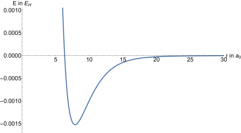
Figure 2: Interaction potential of two Li atoms in the lowest triplet state. This atomic interaction potential is used as a prototype realistic atom-atom interaction potential.

In the ultracold regime, the isotropic short-range interaction can be parameterised by the $s$-wave scattering length $a_{\rm sc}$ which is determined by the energy of the most weakly bound state. In order to simulate, e. g., the variation of the scattering length in the vicinity of a magnetic Feshbach resonance or a different system of particles, the approach described in [34] is used where a small modification of the inner wall of the potential varies the position of the last bound state and hence the $s$-wave scattering length in the absence of the DDI.

However, it is important to note that the concept of the $s$-wave scattering length breaks down for a non-zero dipole moment. First, a partial-wave expansion does not decouple the wavefunction with respect to the angular momentum quantum number $l$, since the DDI couples all even (odd) $l$ quantum numbers. Second, the $1/r^{3}$ tail of the DDI leads besides the usual linear term also to a logarithmic term in the asymptotic part of the wavefunction [24]. This logarithmic behaviour cannot be described by short-range $s$-wave scattering.

4.1 Isotropic harmonic trapping potential

First, we consider an isotropic harmonic confinement. The harmonic potential

$$\begin{split}V_{i}(\mathbb{r_{i}})=\sum_{j=x_{i},y_{i},z_{i}}V_{0,j}k_{j}^{2}j^{2}\;\end{split}$$ (24)

is obtained by a Taylor expansion of the optical-lattice potential truncated at second order. Introducing the harmonic oscillator frequencies $\omega=\sqrt{\frac{2V_{0}k^{2}}{\mu}}$ and $\Omega=\sqrt{\frac{4V_{0}k^{2}}{M}}$ where $M=m_{1}+m_{2}=2m$, the potential

$$\begin{split}V_{i}(\mathbb{r_{i}})&=V_{\rm rm}(r)\;\;+\;V_{\rm CM}(R)=\frac{1}{2}\mu\omega^{2}r^{2}+\frac{1}{2}M\Omega^{2}R^{2}\end{split}$$ (25)

is separable in relative and center-of-mass coordinates, i. e. the coupling term $\hat{\rm W}(\mathbb{r},\mathbb{R})$ vanishes. Since additionally the DDI affects only the relative-motion coordinates, the center-of-mass Hamiltonian is the one of an ordinary harmonic oscillator. Thus, we concentrate on the relative-motion Hamiltonian in Eq. (14).

The total energy spectrum can be characterised by two different energy regimes. In the bound-state regime, i. e. the energy range below the dissociation threshold in the absence of a trap, the characteristic energies are on the order of the energies of the interaction potential $V_{\mathrm{sh}}$ that supports bound rovibrational states. In the trap-state regime, i. e. for the states above the dissociation threshold in the absence of a trap, the characteristic energies are on the order of the trap-discretized continuum states that we denote as trap states in the following. In our case, the typical trap-state energies are of the order of a few $\hbar\omega$ which corresponds in atomic units to about $10^{-12}E_{H}$. The characteristic depth of the short-range potential $V_{\rm sh}$ is about $-10^{9}\hbar\omega$. The typical energy difference of the vibrational levels in units of $\hbar\omega$ is approximately $10^{8}\hbar\omega$. Also the characteristic energy difference of the rotational energy levels of about $10^{7}\hbar\omega$ is orders of magnitude larger compared with the characteristic energy scales of a few $\hbar\omega$ in the trap-state regime. Therefore, the two regimes will be discussed separately in the following two subsections.

4.1.1 Bound-state regime.

First the bound-state regime is considered. Since we adopt a realistic interaction potential there exist more than one bound state. These bound states can couple to each other due to the DDI.

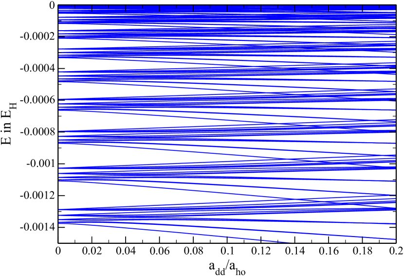
Figure 3: Relative-motion energy spectrum for the $A_{g}$ symmetry of the $D_{2h}$ point group showing the bound regime of the energy spectrum for variable dipolar interaction strength.

Fig. 3 shows the energy spectrum of the $A_{g}$ symmetry of two identical dipolar particles in an isotropic harmonic trap interacting via the short-range interaction potential (Fig. 2) as a function of the dipole interaction strength of the DDI, which is characterised by the ratio between the dipole-length $a_{\rm dd}=\frac{\mu C_{\rm dd}}{4\pi\hbar^{2}}$ and the harmonic oscillator length $a_{\rm ho}$. Since the $A_{g}$ symmetry is gerade, the spectrum represents identical bosons. The dipolar interaction strength $\frac{a_{\rm dd}}{a_{\rm ho}}$ determines the behaviour of the system in the long-range regime. In Fig. 3 groups of states appear which are partly degenerate at $\frac{a_{\rm dd}}{a_{\rm ho}}=0$ and begin to separate for increasing dipole interaction strength. Each group of states corresponds to one vibrational energy level and its rotational excitations. In total there are eleven vibrational states supported by the short-range potential shown in Fig. 2. In the calculation the number of rotational excitations for each vibrational energy level is limited by the number $N_{l}$ of the basis set in Eq. (18).

The group of states in the energy interval between $E=-0.0014\;E_{H}$ and $E=-0.0012\;E_{H}$ corresponds to the vibrational ground state and its rotational excitations. The next set of states between $E=-0.0012\;E_{H}$ and $E=-0.0010\;E_{H}$ corresponds to the first excited vibrational state and its rotational energy levels. For each set of rovibrational states the properties are similar. As is visible from Fig. 3, the different rovibrational states of each set respond differently to the increasing dipole interaction strength. Since the head-to-tail configuration corresponds to states with the rotational quantum numbers $m=0$, these states decrease in energy with increasing dipole interaction strength. The states in the side-by-side configuration correspond to $l=|m|\neq 0$ quantum numbers and increase in energy for increasing dipole interaction strength. The rovibrational ground state at $E\approx-0.00137\;E_{H}$ changes most strongly with the DDI, since the expectation value of $\bar{r}=\left<\varphi\vphantom{r\varphi}\right|r\left|\varphi\vphantom{\varphi r}\right>$ is the smallest and therefore the DDI matrix elements are the largest, because the dipole-dipole matrix elements scale as $r^{-3}$. With increasing vibrational excitation $\bar{r}$ gets larger and the splitting of the different rovibrational states is weaker.

Figure 4: Magnified view on Fig. 3 that shows the different behaviour of the rovibrational levels with increasing dipole interaction strength.

In Fig. 4 the different splittings of the first two sets of rovibrational states are shown in an enlarged view compared to Fig. 3. In the present calculation the basis set is includes only l quantum numbers up to $N_{l}=8$. Since only even numbers of $l$ and $m$ are allowed in the gerade $A_{g}$ case, there are five values of $l$ contained in the basis and the number of rotational states per vibrational level visible in Fig. 4 is correspondingly limited to this number. The $m$ degeneracy of the rotational levels is lifted because the DDI breaks the spherical symmetry. From an analysis of the wavefunction of the deeply bound states the general properties of the states becomes evident, see Fig. 5. While the $m$ quantum number is preserved, the $l$ quantum numbers are coupled by the DDI. Therefore, each state consists of a fixed $m$ quantum number with contributions from all even $l$ quantum numbers. On this basis it is possible to judge whether a state belongs dominantly to the head-to-tail or the side-by-side configuration or is in between these extremes. In general, the states with $m=0$ correspond to the classical head-to-tail configuration and states with $|m|>0$ represent more the side-by-side configuration, especially the states with $l=|m|\neq 0$ have a pronounced side-by-side geometry.

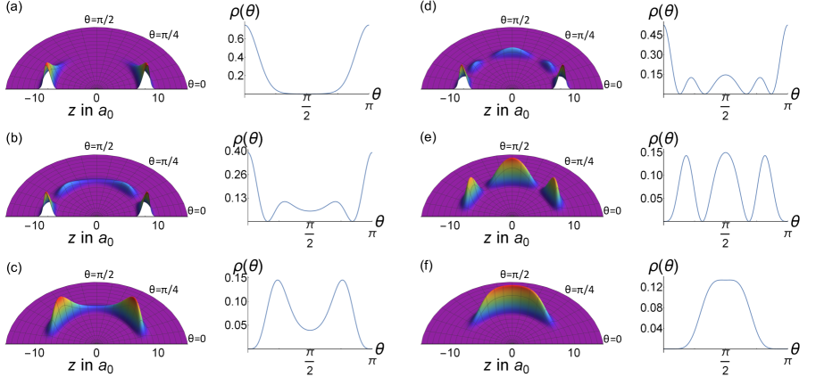
Figure 5: Pair densities $\rho(r,\theta,\phi=0)$ of the 6 energetically lowest lying bound states (sorted from (a) to (f)) for the dipole interaction strength $\frac{a_{\rm dd}}{a_{\rm ho}}=0.025$. The solutions of the full Hamiltonian in Eq. (3) (3D plots) are compared to the ones of the model Hamiltonian in Eq. (26) (2D plots).

In Fig. 5 the pair densities of the vibrational ground state with its rotational excitations are shown. These pair densities do not possess a vibrational excitation as can be seen from the missing nodes in the radial part of the pair densities. For the excited rotational states Fig. 5(b) to (f) additional nodes appear in the angular part of the pair densities. Moreover, the states in Fig. 5(a), (b), and (d) corresponds to the head-to-tail configuration, since the probability for two dipolar particles to stand on top of each other is the largest. In contrast, the state in Fig. 5(c) does not show a clear side-by-side or head-to-tail configuration as it has minima in both cases. The state in Fig. 5(f) has a maximum for the side-by-side configuration and increases in energy for an increasing dipole interaction strength, as described above and visible from Fig. 4. Finally, the state shown in Fig. 5(e) has a node for the head-to-tail configuration and some maximum for the side-by-side configuration, but equal maxima for the angle in between.

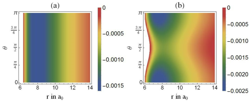
Figure 6: Full interaction potential $V_{\rm int}$ for different interaction strengths $\frac{a_{\rm dd}}{a_{\rm ho}}$. (a) Isotropic case without DDI ($\frac{a_{\rm dd}}{a_{\rm ho}}=0$).(b) Short-range potential with a non-zero DDI ($\frac{a_{\rm dd}}{a_{\rm ho}}=0.15$).

Fig. 6 shows how the total potential $V_{\rm int}$ changes for small particle separations due to the dipolar interaction ($\frac{a_{\rm dd}}{a_{\rm ho}}=0$ or $\frac{a_{\rm dd}}{a_{\rm ho}}\neq 0$ ). The total potential in Fig. 6(b) becomes increasingly anisotropic due to the DDI and dips for the head-to-tail configuration as well as bumps for the side-by-side configuration appear. Since the total potential in Fig. 6(b) is shallower in the $\theta$ direction than in the radial direction, it is more likely to have first excitations in the angular part of the pair densities, see Fig. 5.

In order to better understand the behavior of the pair densities shown in Fig. 5 we consider the model Hamiltonian

$$\begin{split}\hat{\rm H}_{\rm model}=\frac{\hat{\rm L}^{2}}{2\mu r_{0}^{2}}+\frac{C_{\rm dd}}{4\pi}\frac{1-3\cos^{2}(\theta)}{r_{0}^{3}}\end{split}$$ (26)

consisting only of the angular part of the full Hamiltonian Eq. (1) for constant $r=r_{0}$. $r_{0}$ is chosen such that the pair density of the vibrational ground state has its maximum. The solution of the model Hamiltonian in Eq. (26) is obtained by diagonalizing the model Hamiltonian in the basis of spherical harmonics.

In Fig. 5, very good agreement is visible comparing the full solution (3D plots) for constant $r_{0}\approx 8$ with the solution of the model Hamiltonian (2D plots). However, higher excited vibrational states possess a more pronounced $r$ dependence which leads to a more complex radial nodal structure as shown in Fig. 7(a). In this case the simplified model Hamiltonian is hence not expected to reproduce well the radial behaviour.

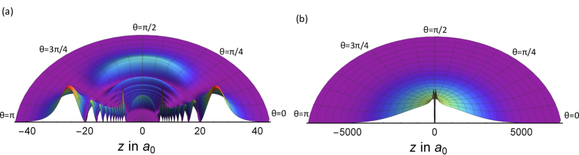
Figure 7: Relative-motion pair density $\rho(r,\theta,0)$ of (a) a bound state close to the interaction potential threshold with $E=-49,283\;\hbar\omega$ at $\frac{a_{\rm dd}}{a_{\rm ho}}=0.01$ and (b) the first trap state with $E=1.488\;\hbar\omega$ for a dipole interaction strength of $\frac{a_{\rm dd}}{a_{\rm ho}}=0.001$

Additionally, there exist metastable states above the trap-free dissociation threshold. In the absence of a DDI such states gain their stability by the centrifugal barrier, but they can dissociate by tunnelling through this barrier. With increasing dipole interaction strength those metastable states strongly respond to the DDI, since the distance of the two dipolar particles is small compared to the inter-particle distance of trap states, see Fig. 7. For increasing DDI, a metastable state can increase (decrease) in energy depending on whether the configuration of the state is dominantly side-by-side (head-to-tail). Similarly, a bound state that is in energy close to the trap-free dissociation threshold for a vanishing DDI can increase in energy above the threshold if it has a predominant side-by-side configuration. In this case the state can surpass the (trap-free) continuum threshold and becomes an unbound or metastable state.

4.1.2 Trap-state regime.

Next, we consider the trap-state regime.

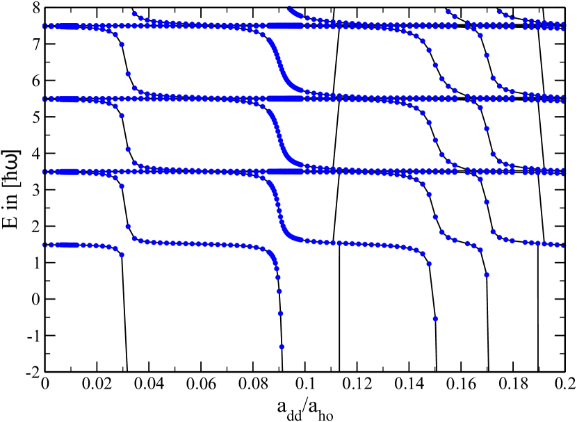
Figure 8: Relative-motion energy spectrum for the $A_{g}$ symmetry of the $D_{2h}$ point group showing the trap-state regime of the energy spectrum as a function of the dipole interaction strength.

The basically horizontal lines in Fig. 8 correspond to the harmonic-oscillator trap states in the diabatic picture. Since this is the energy spectrum of the $A_{g}$ symmetry, only even numbers of $l$ and $m$ are allowed. The energy of two non-interacting particles in a three-dimensional isotropic trap in spherical coordinates is $E_{\rm ho}=(k+3/2)\hbar\omega$, with $k\equiv 2n+l$. Thus the degeneracy of the energy level $k$ is $(k+2)(k+4)/8$ where $k=0,2,4,6...$ are only even numbers due to the $A_{g}$ symmetry. For the even $k$ quantum numbers the spacing of the harmonic-trap states is $2\hbar\omega$ in accordance with the energies shown in Fig. 8.

The almost vertical lines at $\frac{a_{\rm dd}}{a_{\rm ho}}=0.03$, $\frac{a_{\rm dd}}{a_{\rm ho}}=0.09$, $\frac{a_{\rm dd}}{a_{\rm ho}}=0.15$, and $\frac{a_{\rm dd}}{a_{\rm ho}}=0.17$ are bound states that show avoided crossings with the trap-discretized continuum states leading to dipole-induced resonances, see Section 4.1.3. These bound states consist of a mixture all spherical harmonics with different $l$ but equal $m$ quantum numbers. The fact that those bound states appear as almost vertical lines is a consequence of the very different energy scales differing by 7 to 8 orders of magnitude between the bound states and the trap states, as was discussed earlier.

The bound state at $\frac{a_{\rm dd}}{a_{\rm ho}}=0.11$ lies rather close to the dissociation threshold for vanishing DDI and has a predominant side-by-side configuration. This leads to an increasing energy that surpasses the (trap-free) dissociation threshold for a large DDI. The bound state at $\frac{a_{\rm dd}}{a_{\rm ho}}=0.19$ is a metastable state, see Section 4.1.1. Both states do not couple to trap states because of non-agreeing $m$ quantum numbers.

4.1.3 Dipole-induced resonances.

A key feature of the energy spectrum in Fig. 8 is the occurrence of broad scattering resonances, which we denote as dipole-induced resonances (DIR). These resonances manifest as broad avoided crossings in the energy spectrum and are found for $\frac{a_{\rm dd}}{a_{\rm ho}}\approx 0.03$, $\frac{a_{\rm dd}}{a_{\rm ho}}\approx 0.09$, $\frac{a_{\rm dd}}{a_{\rm ho}}\approx 0.15$, and $\frac{a_{\rm dd}}{a_{\rm ho}}\approx 0.17$. They can be understood in the following way. Increasing the dipole interaction strength deepens the interaction potential $V_{\rm int}$ and introduces a new bound state in the inter-particle potential. This bound state crosses in energy with trap states. Due to the dipolar coupling these crossings become avoided. A further increase of the interaction strength repeats this process leading to the series of resonances (avoided crossings) visible in Fig. 8. The resonances shown in [32, 21, 27, 28] seem also to be DIR.

The excited trap states that do not couple to the bound states (e. g. the almost horizontal line at $E\approx 3.5\hbar\omega$) are $l\neq 0$ states. The centrifugal barrier $\frac{\hbar^{2}}{2\mu}\frac{l(l+1)}{r^{2}}$ shields the trap states from noticing the bound state that is much more confined compared to a trap state, see Fig. 7. Due to the shielding effect of the centrifugal barrier for the trap states with $l\neq 0$ there is very little overlap with the bound state. This leads to an almost vanishing coupling.

4.1.4 Dipolar coupling of trap states.

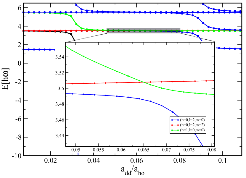
Figure 9: Magnified view on Fig. 8 that shows an avoided crossing between trap states. The quantum numbers in the legend are associated with the quantum numbers of a harmonic oscillator. The indexing of the states with the quantum numbers is only valid far away from the resonance.

An enlarged view of Fig. 8 is shown in Fig. 9. The red state corresponds to a trap state where the dipoles possess a side-by-side configuration. It is well described by a harmonic oscillator state with $(n=0,l=2,m=2)$. Therefore, the energy of this state increases with the dipole interaction strength. Moreover, there is a non-avoided crossing of the red and the green state. The green state is a trap state with quantum numbers $(n=1,l=0,m=0)$. From the selection rules of the DDI (see Section 3.2) it follows that only states with equal $m$ quantum numbers can couple due to the DDI. Consequently, this is a non-avoided crossing of two non-interacting states. Furthermore, there is an avoided crossing between the blue state $(n=0,l=2,m=0)$ and the green state. This is a direct consequence of the selection rules of the DDI. The coupling of the trap states is significantly smaller than the coupling in the DIR, because the coupling matrix element Eq. (22) for two trap states is smaller than for a trap and a bound state. Hence, the coupling matrix element is larger for small $r$, which is the case for the much more strongly confined bound state compared with a trap state. The avoided crossings between trap states can nevertheless be used to adiabatically transfer an isotropic trap state to a polarised one and could thus be used for some control scheme.

4.1.5 Influence of the short-range potential.

To investigate the influence of the short-range potential for dipolar particles, the $s$-wave scattering length of the short-range potential for zero DDI is varied by an inner-wall manipulation [34]. The energy spectra of two dipolar particles interacting via different short-range potentials are shown as a function of the dipole interaction strength in Fig. 10. Each energy spectrum refers to a different $s$-wave scattering length of the bare short-range potential $V_{\mathrm{sh}}$.

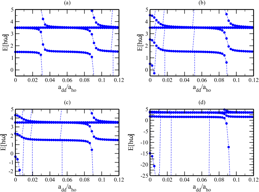
Figure 10: Relative-motion energy spectra for different short-range potentials which correspond to different $s$-wave scattering length $a_{\rm sc}$ for zero dipole interaction strength. This corresponds to either an attractive ($a_{\rm sc}<0$) or a repulsive ($a_{\rm sc}>0$) short-range interaction. Energy spectrum for (a) $\frac{a_{\rm ho}}{a_{\rm sc}}=-100$, (b) $\frac{a_{\rm ho}}{a_{\rm sc}}=0.01$, (c) $\frac{a_{\rm ho}}{a_{\rm sc}}=1.0$, and (d) $\frac{a_{\rm ho}}{a_{\rm sc}}=5.0$.

As in Fig. 8 the horizontal lines correspond to harmonic-trap states. The variation of $V_{\mathrm{sh}}$ changes the position of the DIR as is shown in Tab. 1.

Table 1: Position of the DIRs in Fig. 10.

• Scattering length $a_{\rm sc}\,[a_{0}]$	Position of the	Position of the
  of $V_{\mathrm{sh}}$	first DIR [$a_{\rm dd}/a_{\rm ho}$]	second DIR [$a_{\rm dd}/a_{\rm ho}$]
  -25	0.03	0.09
  250000	0.005	0.09
  25000	0.005	0.09
  500	0.004	0.09

The short-range potential has a strong influence on the position of the first DIR because for small dipole interaction strength $\frac{a_{\rm dd}}{a_{\rm ho}}$ the DDI is negligible. In contrast, the position of the second DIR (at $\frac{a_{\rm dd}}{a_{\rm ho}}=0.09$) is almost unaffected by a manipulation of $V_{\mathrm{sh}}$. For increasing dipole interaction strengths $\frac{a_{\rm dd}}{a_{\rm ho}}$ the DDI becomes dominant compared to the short-range potential $V_{\mathrm{sh}}$. Consequently, the long-range behavior of the wavefunction is not longer affected by changes in $V_{\mathrm{sh}}$. This can be understood on the basis of the different energy shifts for bound states resulting from an inner-wall manipulation compared to the one induced by increasing the DDI. While the energy of the bound states respond sensitively on an inner-wall variation for small DDI, for a large DDI the energy shift due to the inner-wall manipulation is negligible compared to the changes in the vibrational energy levels induced by a variation of the DDI, see, e. g., Fig. 3. It is certainly remarkable that this effect can be used to directly change the position of the first DIR, which allows for controlling and manipulating dipolar quantum gases.

4.2 Anisotropic sextic trapping potential

Every realistic potential is finite and hence certainly anharmonic. Therefore, in the following, the harmonic approximation is abandoned and a sextic potential is considered which has proven to accurately describe center-of-mass to relative motion coupling in single-well potentials [35, 16, 17]. A pancake-shaped trap with an anisotropy of $\frac{\omega_{z}}{\omega_{\bot}}=10$ is adopted. Such a quasi-2D geometry is a common experimental set-up to stabilise a dipolar BEC against collapse [36]. Again, the short-range potential of Li is chosen as a prototype short-range potential $V_{\mathrm{sh}}$. The sextic potential

$$\begin{split}V_{i}(\mathbb{r_{i}})=\sum_{j=x_{i},y_{i},z_{i}}\,V_{j}\left(k_{j}^{2}j^{2}-\frac{1}{3}\,k_{j}^{4}j^{4}+\frac{2}{45}\,k_{j}^{6}j^{6}\right)\;\end{split}$$ (27)

is obtained by a Taylor expansion of a $\sin^{2}$ optical lattice up to the sixth order. While in the harmonic case center-of-mass and relative motion decouple, for a sextic potential the coupling term

$$\begin{split}\hat{\rm W}(\mathbb{r},\mathbb{R})=\sum_{c=x,y,z}V_{0,c}\left(-k_{c}^{4}r_{c}^{2}R_{c}^{2}+\frac{1}{3}k_{c}^{6}r_{c}^{2}R_{c}^{4}+\frac{1}{12}k_{c}^{6}r_{c}^{4}R_{c}^{2}\right)\;\end{split}$$ (28)

does not vanish. Note, the coupling term is non-zero even for a harmonic confinement if the two particles have different products of polarizability and mass. Hence, for the description of the full spectrum the Schrödinger equation of the six-dimensional Hamiltonian Eq. (3) has to be solved which requires to perform the exact diagonalization as described in Section 3.1.

For distinguishable particles the coupling term $W(\mathbb{r},\mathbb{R})$ includes all non-separable parts of the form $r^{n}R^{m}$ with $n,m\in\mathbb{N}\backslash\{0\}$. In the case of identical particles the non-separable parts consists of monomials with even values of $n$ and $m$, such as $r^{2}R^{2}$, $r^{2}R^{4}$, and $r^{4}R^{2}$, see Eq. (28). The matrix elements with the coupling term

$$\begin{split}W_{\alpha,\beta}=\left<\Phi^{(\alpha)}(\mathbf{r},\mathbf{R})\vphantom{\hat{\rm W}(\mathbf{r},\mathbf{R})\Phi^{(\beta)}(\mathbf{r},\mathbf{R})}\right|\hat{\rm W}(\mathbf{r},\mathbf{R})\left|\Phi^{(\beta)}(\mathbf{r},\mathbf{R})\vphantom{\Phi^{(\alpha)}(\mathbf{r},\mathbf{R})\hat{\rm W}(\mathbf{r},\mathbf{R})}\right>\end{split}$$ (29)

couple configurations $\Phi$ with gerade or ungerade symmetry for even values of $n$ and $m$. The energy spectra shown in Fig. 11 were calculated for two dipolar particles in an anisotropic sextic trapping potential with the interaction potential discussed before as a function of the dipole interaction strength $\frac{a_{\rm dd}}{a_{\rm ho}}$.

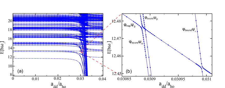
Figure 11: (a) CI spectrum for two aligned dipolar particles for an anisotropic sextic trapping potential with the same short-range potential as in Fig. 8. (b) Magnified view of Fig. 11 resolving avoided and non-avoided crossings.

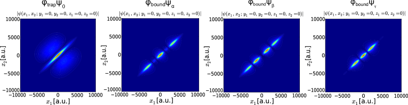
Figure 12: Cuts through the 6-dimensional wavefunctions shown in the energy spectrum in Fig. 11(b). Cuts for $y_{1}=0,y_{2}=0,z_{1}=0,z_{2}=0$ are displayed. From left to right the cuts, beginning with $\varphi_{\rm trap}\;\psi_{0}$ according to the labelling in Fig. 11, are shown.

The major difference between the complete energy spectra for the sextic trap compared with the relative-motion spectrum in the harmonic case is evidently the appearance of the additional center-of-mass excitations. While they are present also in the harmonic case, they do not couple to the relative motion and can thus be considered separately. This is not the case for the sextic trap with coupling. Hence, in the spectrum containing the center-of-mass excitations (Fig. 11) many more states appear. The configurations of the excited center-of-mass motion bound states $\varphi_{\rm bound}(\mathbb{r})\psi_{0}^{(\rm ex)}(\mathbb{R})$ cause a very dense area shown in Fig. 11(a) for a dipole interaction strength of about $\frac{a_{\rm dd}}{a_{\rm ho}}\approx 0.03$. By including more configurations this area continues for dipole interaction strengths above $\frac{a_{\rm dd}}{a_{\rm ho}}\approx 0.03$. However, in the present calculation of the energy spectrum only the relevant configurations are included, which means only those with small energies of a few $\hbar\omega$ are considered. In Fig. 11(b) a magnified view of Fig. 11(a) is shown in which avoided crossings at $\frac{a_{\rm dd}}{a_{\rm ho}}\approx 0.030857$ and $\frac{a_{\rm dd}}{a_{\rm ho}}\approx 0.030958$ can clearly be identified. Also a non-avoided (true) crossing next to the first avoided crossing at $\frac{a_{\rm dd}}{a_{\rm ho}}\approx 0.0309$ is visible.

In the energy spectrum center-of-mass excited bound states cross with trap states. The anharmonicity in the external potential leads to a non-vanishing center-of-mass to relative motion coupling. Hence, these crossings are avoided for certain symmetries of the crossing states. At the avoided crossing, relative-motion binding energy can be transferred into center-of-mass excitation energy due to the anharmonicity in the external confinement. Since this is an inelastic process, we denote these resonances as inelastic confinement-induced dipolar resonances (ICIDR).

These resonances are the dipolar analog for the Feshbach-type resonances induced by a coupling of center-of-mass to relative motion systems of ultracold atoms without DDI [37, 38, 39, 14, 40, 41, 42]. We follow the notation introduced in [16, 17] and denote these resonances as inelastic confinement-induced resonances (ICIR). In complete analogy, also in the dipolar gases resonances appear due to the coupling of center-of-mass excited bound states and trap states with lower center-of-mass excitation for a non-zero coupling term $W$. The difference between ICIR and ICIDR is that the adiabatic transformation of a trap state into a bound state is performed by a change of the scattering length (for example using a magnetic Feshbach resonance) or the geometry of the external confinement in the case of ICIR and by a variation in dipolar interaction strength in the case of ICIDR. Moreover, for ultracold atoms there exists only a single least bound state and the scattering length is determined by its position. Hence, for a specific center-of-mass excitation only a single resonance (with the lowest trap state) exists in the case of ICIR. In contrast, there exists an entire series of bound states for increasing dipolar interaction strength. Hence, a complete series of resonances (with the lowest trap state) exist for each center-of-mass excitation in the case of ICIDR.

To understand the behaviour of the ICIDR in more detail, we investigate the states labelled in Fig. 11(b). The corresponding states may be expressed by their 6-dimensional wavefunctions in absolute coordinates. Representative cuts through the 6D wavefunctions are shown in Fig. 12. Since the trapping potential is rather anisotropic $\frac{\omega_{z}}{\omega_{\bot}}=10$, the lowest energies correspond to states which have excitations in the $x$ and $y$ directions, because the trap is shallower in these directions compared to the tight $z$ direction. In Fig. 12 the wavefunction $\varphi_{\rm bound}\psi_{\beta}$ is shown. This state has a node at $(x_{1}=0,x_{2}=0)$ and does not interact with the state $\varphi_{\rm trap}\psi_{0}$. Hence the coupling term from equation Eq. (29) has an anti-symmetric integrand and therefore the total integral vanishes. The vanishing coupling term

$$\begin{split}\left<\varphi_{\rm trap}\;\psi_{0}\vphantom{\hat{\rm W}(\mathbf{r},\mathbf{R})\varphi_{\rm bound}\;\psi_{\beta}}\right|\hat{\rm W}(\mathbf{r},\mathbf{R})\left|\varphi_{\rm bound}\;\psi_{\beta}\vphantom{\varphi_{\rm trap}\;\psi_{0}\hat{\rm W}(\mathbf{r},\mathbf{R})}\right>=0\end{split}$$ (30)

leads to a non-avoided crossing between the states $\varphi_{\rm trap}\;\psi_{0}$ and $\varphi_{\rm bound}\;\psi_{\beta}$. Moreover, the trap state $\varphi_{\rm trap}\psi_{0}$ and the center-of-mass excited bound state $\varphi_{\rm bound}\psi_{\alpha}$ have a non-vanishing coupling term, since these states have the same symmetry, which can be seen from the nodal structure of the cuts through the wavefunctions in Fig. 12. From Fig. 12 it can be concluded that solely states which have an even (odd) nodal structure can couple to each other. Otherwise the wavefuntions have different symmetries, i. e. gerade and ungerade. This results in a vanishing coupling term in Eq. (29), because the total integrand is anti-symmetric. It is important to note that it has been demonstrated that the coupling of trap states to center-of-mass excited bound states at an ICIR has lead to massive atom losses and heating in a cloud of Cs atoms [18] due to molecule formation [16, 17]. As a consequence, it is expected that an ICIDR influences the stability of dipolar quantum gases as well.

5 Summary and Conclusion

An approach is presented that allows for the numerical description of two ultra-cold particles interacting via an arbitrary isotropic short-range interaction and the long-range, anisotropic DDI confined to a finite orthorhombic 3D optical lattice. The coupling between center-of-mass and relative motion coordinates is incorporated in a configuration-interaction manner and hence the full 6D problem is solved. A key feature is the use of a realistic inter-particle interaction potential, e. g. numerically provided Born-Oppenheimer potential curves. The orthorhombic symmetry of the problem, preserved by the dipole-dipole interaction, and the quantum statistics (distinguishable particles as well as identical bosons or fermions) are explicitly incorporated in the approach.

With the here presented approach a system of two dipolar particles interacting via a short-range potential trapped in a single well of an optical lattice was investigated. It is shown that various resonances occur in these systems. The dipole-induced resonances occur due to the change of the total interaction potential and thus the bound-state spectrum as a result of a change of the dipole interaction strength. Furthermore, the existence of dipolar coupling resonances of trap states is demonstrated. The position of specific resonances can be precisely manipulated by a manipulation of the short-range potential by, e. g., a magnetic Feshbach resonance. This provides additional tools for controlling and manipulating trapped dipolar quantum gases. This has the potential to provide advanced cooling schemes, by, e. g., performing adiabatic and diabatic changes of the dipole interaction strength.

In addition, the occurrence of inelastic confinement-induced dipolar resonances (ICIDR) due to a coupling of center-of-mass and relative motion is demonstrated. The mechanism of these resonances is universal and in analogy to inelastic confinement-induced resonances of ultracold atoms [16, 17] and Coulomb interacting system like quantum dots [43].

As a straightforward extension, the interaction potential of two non-aligned dipoles is planned. This includes all spherical harmonics $V_{\rm dd}\propto\sum_{q=-2}^{2}Y_{2}^{q}$. This leads to a coupling of both $l$ and $m$ quantum numbers and therefore an even richer energy spectrum with much more resonances is expected to be found.

Bibliography

Bibliography

- [1] W.C. Stwalley. Efficient conversion of ultracold Feshbach-resonance-related polar molecules into ultracold ground state (X molecules. Eur. Phys. J. D, 31:221–225, 2004.
- [2] Wenhui Li, Paul J. Tanner, and T. F. Gallagher. Dipole-Dipole Excitation and Ionization in an Ultracold Gas of Rydberg Atoms. Phys. Rev. Lett., 94:173001, 2005.
- [3] M.A. Baranov, M. Dalmonte, G. Pupillo, and P. Zoller. Condensed matter theory of dipolar quantum gases. Chem. Rev., 112:5012–5061, 2012.
- [4] T. Lahaye, C. Menotti, L. Santos, M. Lewenstein, and T. Pfau. The physics of dipolar bosonic quantum gases. Rep. Prog. Phys., 72:126401, 2009.
- [5] S. Ospelkaus, A. Pe’Er, K.-K. Ni, J.J. Zirbel, B. Neyenhuis, S. Kotochigova, P.S. Julienne, J. Ye, and D.S. Jin. Efficient state transfer in an ultracold dense gas of heteronuclear molecules. Nat. Phys., 4:622–626, 2008.
- [6] K.-K. Ni, S. Ospelkaus, M. H. G. de Miranda, A. Pe’er, B. Neyenhuis, J. J. Zirbel, S. Kotochigova, P. S. Julienne, D. S. Jin, and J. Ye. A High Phase-Space-Density Gas of Polar Molecules. Science, 322:231–235, 2008.
- [7] J. Deiglmayr, A. Grochola, M. Repp, K. Mörtlbauer, C. Glück, J. Lange, O. Dulieu, R. Wester, and M. Weidemüller. Formation of Ultracold Polar Molecules in the Rovibrational Ground State. Phys. Rev. Lett., 101:133004, 2008.
- [8] J. Stuhler, A. Griesmaier, T. Koch, M. Fattori, T. Pfau, S. Giovanazzi, P. Pedri, and L. Santos. Observation of Dipole-Dipole Interaction in a Degenerate Quantum Gas. Phys. Rev. Lett., 95:150406, 2005.
- [9] Axel Griesmaier, Jörg Werner, Sven Hensler, Jürgen Stuhler, and Tilman Pfau. Bose-Einstein Condensation of Chromium. Phys. Rev. Lett., 94:160401, 2005.
- [10] Mingwu Lu, Nathaniel Q. Burdick, Seo Ho Youn, and Benjamin L. Lev. Strongly Dipolar Bose-Einstein Condensate of Dysprosium. Phys. Rev. Lett., 107:190401, 2011.
- [11] K. Aikawa, A. Frisch, M. Mark, S. Baier, A. Rietzler, R. Grimm, and F. Ferlaino. Bose-Einstein Condensation of Erbium. Phys. Rev. Lett., 108:210401, 2012.
- [12] D. DeMille. Quantum Computation with Trapped Polar Molecules. Phys. Rev. Lett., 88:067901, 2002.
- [13] Philipp-Immanuel Schneider and Alejandro Saenz. Quantum computation with ultracold atoms in a driven optical lattice. Phys. Rev. A, 85:050304, 2012.
- [14] Philipp-Immanuel Schneider, Sergey Grishkevich, and Alejandro Saenz. Ab initio determination of Bose-Hubbard parameters for two ultracold atoms in an optical lattice using a three-well potential. Phys. Rev. A, 80:013404, 2009.
- [15] M.L. Wall and L.D. Carr. Dipole–dipole interactions in optical lattices do not follow an inverse cube power law. New J. Phys., 15:123005, 2013.
- [16] Simon Sala, Philipp-Immanuel Schneider, and Alejandro Saenz. Inelastic confinement-induced resonances in low-dimensional quantum systems. Phys. Rev. Lett., 109:073201, 2012.
- [17] S Sala, G Zürn, T Lompe, A.N. Wenz, S Murmann, F Serwane, S Jochim, and A Saenz. Coherent molecule formation in anharmonic potentials near confinement-induced resonances. Phys. Rev. Lett., 110:203202, 2013.
- [18] Elmar Haller, Manfred J. Mark, Russell Hart, Johann G. Danzl, Lukas Reichsöllner, Vladimir Melezhik, Peter Schmelcher, and Hanns-Christoph Nägerl. Confinement-induced resonances in low-dimensional quantum systems. Phys. Rev. Lett., 104:153203, 2010.
- [19] S. Yi and L. You. Trapped atomic condensates with anisotropic interactions. Phys. Rev. A, 61:041604, 2000.
- [20] S. Yi and L. You. Trapped condensates of atoms with dipole interactions. Phys. Rev. A, 63:053607, 2001.
- [21] Zhe-Yu Shi, Ran Qi, and Hui Zhai. -wave-scattering resonances induced by dipolar interactions of polar molecules. Phys. Rev. A, 85:020702, 2012.
- [22] M. Olshanii. Atomic scattering in the presence of an external confinement and gas of impenetrable Bosons. Phys. Rev. Lett., 81:938, 1998.
- [23] T. Bergeman, M. G. Moore, and M. Olshanii. Atom-atom scattering under cylindrical harmonic confinement: Numerical and analytic studies of the confinement induced resonance. Phys. Rev. Lett., 91:163201, 2003.
- [24] S. Sinha and L. Santos. Cold Dipolar Gases in Quasi-One-Dimensional Geometries. Phys. Rev. Lett., 99:140406, 2007.
- [25] Tao Shi and Su Yi. Observing dipolar confinement-induced resonances in quasi-one-dimensional atomic gases. Phys. Rev. A, 90:042710, 2014.
- [26] Sergey Grishkevich, Simon Sala, and Alejandro Saenz. Theoretical description of two ultracold atoms in finite three-dimensional optical lattices using realistic interatomic interaction potentials. Phys. Rev. A, 84:062710, 2011.
- [27] Shai Ronen, Daniele C.E. Bortolotti, D. Blume, and John L. Bohn. Dipolar Bose-Einstein condensates with dipole-dependent scattering length. Phys. Rev. A, 74:033611, 2006.
- [28] D.C.E. Bortolotti, S. Ronen, J.L. Bohn, and D. Blume. Scattering length instability in dipolar bose-einstein condensates. Phys. Rev. Lett., 97:160402, 2006.
- [29] N. Bartolo, D.J. Papoular, L. Barbiero, C. Menotti, and A. Recati. Dipolar-induced resonance for ultracold bosons in a quasi-one-dimensional optical lattice. Phys. Rev. A, 88:023603, 2013.
- [30] Shi-Guo Peng, Hui Hu, Xia-Ji Liu, and Peter D. Drummond. Confinement-induced resonances in anharmonic waveguides. Phys. Rev. A, 84:043619, 2011.
- [31] Immanuel Bloch. Ultracold quantum gases in optical lattices. Nat. Phys., 1:23, 2005.
- [32] K. Kanjilal and D. Blume. Low-energy resonances and bound states of aligned bosonic and fermionic dipoles. Phys. Rev. A, 78:040703, 2008.
- [33] Sergey Grishkevich and Alejandro Saenz. Influence of a tight isotropic harmonic trap on photoassociation in ultracold homonuclear alkali-metal gases. Phys. Rev. A, 76:022704, 2007.
- [34] Sergey Grishkevich, Philipp-Immanuel Schneider, Yulian V. Vanne, and Alejandro Saenz. Mimicking multichannel scattering with single-channel approaches. Phys. Rev. A, 81:022719, 2010.
- [35] Sergey Grishkevich and Alejandro Saenz. Theoretical description of two ultracold atoms in a single site of a three-dimensional optical lattice using realistic interatomic interaction potentials. Phys. Rev. A, 80:013403, 2009.
- [36] Tobias Koch, Thierry Lahaye, Jonas Metz, Bernd Fröhlich, Axel Griesmaier, and Tilman Pfau. Stabilization of a purely dipolar quantum gas against collapse. Nat. Phys., 4:218–222, 2008.
- [37] E. L. Bolda, E. Tiesinga, and P. S. Julienne. Ultracold dimer association induced by a far-off-resonance optical lattice. Phys. Rev. A, 71:033404, 2005.
- [38] V. Peano, M. Thorwart, C. Mora, and R. Egger. Confinement-induced resonances for a two-component ultracold atom gas in arbitrary quasi-one-dimentional traps. New J. Phys., 7:192, 2005.
- [39] Vladimir Melezhik and Peter Schmelcher. Quantum dynamics of resonant molecule formation in waveguides. New Journal of Physics, 11(7):073031, 2009.
- [40] J. P. Kestner and L-M. Duan. Anharmonicity-induced resonances for ultracold atoms and their detection. New J. Phys., 12:053016, 2010.
- [41] G. Lamporesi, J. Catani, G. Barontini, Y. Nishida, M. Inguscio, and F. Minardi. Scattering in mixed dimensions with ultracold gases. Phys. Rev. Lett., 104:153202, 2010.
- [42] Manuel Valiente and Klaus Mølmer. Quasi-one-dimensional scattering in a discrete model. Phys. Rev. A, 84:053628, 2011.
- [43] Maria Troppenz, Simon Sala, Philipp-Immanuel Schneider, and Alejandro Saenz. Inelastic confinement-induced resonances in quantum dots. (in preparation).