Efimov Physics in Cold Atoms

Abstract

Atoms with a large scattering length have universal low-energy properties that do not depend on the details of their structure or their interactions at short distances. In the 2-atom sector, the universal properties are familiar and depend only on the scattering length. In the 3-atom sector for identical bosons, the universal properties include the existence of a sequence of shallow triatomic molecules called Efimov trimers and log-periodic dependence of scattering observables on the energy and the scattering length. In this review, we summarize the universal results that are currently known. We also summarize the experimental information that is currently available with an emphasis on 3-atom loss processes.

1 Introduction

The scattering of two particles with sufficiently low kinetic energy is determined by their S-wave scattering length, which is commonly denoted by $a$. The energies of the particles are sufficiently low if their de Broglie wavelengths are large compared to the range of the interaction. The scattering length $a$ is also the most important interaction variable for 3-body systems and for higher $N$-body systems if all their constituents have sufficiently low energy.

Generically, the scattering length $a$ is comparable in magnitude to the range $r_{0}$ of the interaction: $|a|\sim r_{0}$. In exceptional cases, the scattering length can be much larger in magnitude than the range: $|a|\gg r_{0}$. Such a large scattering length requires the fine-tuning of a parameter characterizing the interactions to the neighborhood of a critical value at which $a$ diverges to $\pm\infty$. If the scattering length is large, the atoms exhibit properties that depend on $a$ but are insensitive to the range and other details of the short-range interaction. We will refer to these properties as universal, because they apply equally well to any nonrelativistic particle with short range interactions that produce a large scattering length.

In the 2-body sector, the universal properties are simple but nontrivial. For example, in the case of equal-mass particles with $a>0$, there is a 2-body bound state near the scattering threshold with binding energy $E_{D}=\hbar^{2}/(ma^{2})$. The corrections to this formula are parametrically small: they are suppressed by powers of $r_{0}/a$.

In the 3-body sector, the universal properties are much more intricate. The first strong evidence for universal behavior in the 3-body system was the discovery of the Efimov effect by Vitaly Efimov in 1969 [1]. In the resonant limit $a\to\pm\infty$, there is a 2-body bound state exactly at the 2-body scattering threshold $E=0$. Efimov showed that in this limit there can also be infinitely many, arbitrarily-shallow 3-body bound states whose binding energies $E_{T}^{(n)}$ have an accumulation point at $E=0$. They are called Efimov states. As the threshold is approached, the ratio of the binding energies of successive Efimov states approaches a universal constant. In the case of identical bosons, the asymptotic ratio is

$$E_{T}^{(n+1)}/E_{T}^{(n)} \longrightarrow 1/515.03\,,\qquad{\rm as\ }n\to+\infty{\rm\ \ with\ }a=\pm\infty\,.$$ (1)

The universal ratio in Eq. (1) is independent of the mass or structure of the identical particles and independent of the form of their short-range interactions. The Efimov effect can also occur in other 3-body systems if at least two of the three pairs have a large S-wave scattering length. The numerical value of the asymptotic ratio may differ from the value in Eq. (1). Efimov’s discovery was at first greeted with some skepticism. However the theoretical evidence for the Efimov effect quickly became conclusive.

The Efimov effect proved to be just the first nugget from a gold mine of universal aspects of the 3-body problem. This system has universal properties not only in the resonant limit $a=\pm\infty$, but whenever the scattering length is large compared to the range $r_{0}$. In two brilliant papers in 1971 and 1979 [2, 3], Efimov derived a number of universal results on low-energy 3-body observables for three identical bosons. The dependence of these results on the scattering length or the energy is characterized by scaling behavior modulo coefficients that are log-periodic functions. This behavior is characteristic of a system with a discrete scaling symmetry. We will refer to universal aspects associated with a discrete scaling symmetry as Efimov physics.

Although the existence of Efimov states quickly became well-established theoretically, their experimental confirmation has proved to be more challenging. Although more than 36 years have elapsed since Efimov’s discovery, there has still not been any convincing direct observation of an Efimov state. One promising system for observing Efimov states is ⁴He atoms, which have a scattering length that is more than a factor of 10 larger than the range of the interaction. Calculations using accurate potential models indicate that the system of three ⁴He atoms has two 3-body bound states or trimers. The ground-state trimer is interpreted by some (including the authors) as an Efimov state, and it has been observed in experiments involving the scattering of cold jets of ⁴He atoms from a diffraction grating [4]. The excited trimer is universally believed to be an Efimov state, but it has not yet been observed.

The rapid development of the field of cold atom physics has opened up new opportunities for the experimental study of Efimov physics. This is made possible by two separate technological developments. One is the technology for cooling atoms to the extremely low temperatures where Efimov physics plays a dramatic role. The other is the technology for controlling the interactions between atoms. By tuning the magnetic field to a Feshbach resonance, the scattering lengths of the atoms can be made arbitrarily large. Both of these technological developments were crucial in a recent experiment that provided the first indirect evidence for the existence of an Efimov state [5]. The signature of the Efimov state was a resonant enhancement of the loss rate from 3-body recombination in an ultracold gas of ¹³³Cs atoms.

This experiment is just the beginning of the study of Efimov physics in ultracold atoms. We have recently written a thorough review of universality in few-body physics with large scattering length [6]. In this shorter review, we summarize the results derived in Ref. [6], include a few more recent developments, and focus more directly on applications in atomic physics.

In Section 2, we introduce various scattering concepts that play an important role in Efimov physics. Most of this review is focused on identical bosons, because this is the simplest case in which Efimov states arise and because it is the system for which Efimov physics has been most thoroughly explored. In Section 3 and 4, we summarize the universal features of identical bosons with a large scattering length in the 2-body and 3-body sectors, respectively. In Section 5, we describe the effects of deep diatomic molecules on the universal results. In Section 6, we describe applications to ⁴He atoms and to alkali atoms near a Feshbach resonance. In Section 7, we discuss the conditions under which Efimov physics arises in systems other than identical bosons. In Section 8, we consider the corrections to the universal results from the nonzero effective range and from microscopic models of the atoms as well as the extension of universality to 4-body systems. We conclude with the outlook for the study of Efimov physics in ultracold atoms.

2 Scattering Concepts

2.1 Scattering length

The elastic scattering of two atoms of mass $m$ and total kinetic energy $E=\hbar^{2}k^{2}/m$ can be described by a stationary wave function $\psi({\bm{r}})$ that depends on the separation vector ${\bm{r}}$ of the two atoms. Its asymptotic behavior as $r\to\infty$ is the sum of a plane wave and an outgoing spherical wave:

$$\psi({\bm{r}})\longrightarrow e^{ikz}+f_{k}(\theta){e^{ikr}\over r}\,,$$ (2)

where $f_{k}(\theta)$ is the scattering amplitude, which depends on the scattering angle $\theta$ and the wave number $k$. The differential cross section $d\sigma/d\Omega$ for the scattering of identical bosons can be expressed in the form

$$\frac{d\sigma}{d\Omega}=\left|f_{k}(\theta)+f_{k}(\pi-\theta)\right|^{2}\,.$$ (3)

If the two atoms are identical fermions, the $+$ should be replaced by $-$. If they are distinguishable atoms, the term $+f_{k}(\pi-\theta)$ should be omitted. The elastic cross section $\sigma(E)$ is obtained by integrating over only ${1\over 2}$ the $4\pi$ solid angle if the two atoms are identical bosons or identical fermions and over the entire $4\pi$ solid angle if they are distinguishable.

The partial-wave expansion resolves the scattering amplitude $f_{k}(\theta)$ into contributions from definite angular momentum quantum number $L$ by expanding it in terms of Legendre polynomials of $\cos\theta$:

$$f_{k}(\theta)=\sum_{L=0}^{\infty}{2L+1\over k\cot\delta_{L}(k)-ik}P_{L}(\cos\theta)\,,$$ (4)

If there are no inelastic 2-body channels, the phase shifts $\delta_{L}(k)$ are real-valued. If there are inelastic channels, the phase shifts can be complex-valued with positive imaginary parts.

If the atoms interact through a short-range 2-body potential, then the phase shift $\delta_{L}(k)$ approaches zero like $k^{2L+1}$ in the low-energy limit $k\to 0$. Thus S-wave ($L=0)$ scattering dominates in the low-energy limit unless the atoms are identical fermions, in which case P-wave ($L=1)$ scattering dominates. At sufficiently low energies, the S-wave phase shift $\delta_{0}(k)$ can be expanded in powers of $k^{2}$ [7]. The expansion is called the effective-range expansion and is conventionally expressed in the form

$$k\cot\delta_{0}(k)=-1/a+\mbox{$1\over 2$}r_{s}k^{2}+\ldots\,,$$ (5)

where $a$ is the scattering length and $r_{s}$ the S-wave effective range.

2.2 Natural low-energy length scale

At sufficiently low energies, atoms behave like point particles with short-range interactions. The length scale that governs the quantum behavior of the center-of-mass coordinate of an atom is the de Broglie wavelength $\lambda=2\pi\hbar/p$, where $p$ is the momentum of the atom. If the relative momentum $p$ of two atoms is sufficiently small, their de Broglie wavelengths are larger than the spacial extent of the atoms and they are unable to resolve each other’s internal structure. Their interactions will therefore be indistinguishable from those of point particles. If the atoms interact through a short-range potential with range $r_{0}$ and if the relative momentum of the two atoms satisfies $p\ll\hbar/r_{0}$, then their de Broglie wavelengths prevent them from resolving the structure of the potential.

For real atoms, the potential is not quite short-range. The interatomic potential $V(r)$ between two neutral atoms in their ground states consists of a short range potential and a long-range tail provided by the van der Waals interaction:

$$V(r)\longrightarrow-{C_{6}\over r^{6}}\qquad\mbox{ as\ }r\to\infty\,.$$ (6)

The van der Waals tail of the potential does not prevent the scattering amplitude from being expanded in powers of the relative momentum ${\bm{k}}$, but at 4^th order the dependence on ${\bm{k}}$ becomes nonpolynomial. The coefficient $C_{6}$ determines a length scale called the van der Waals length:

$$\ell_{\rm vdW}=\left(mC_{6}/\hbar^{2}\right)^{1/4}\,.$$ (7)

At sufficiently low energy, the interactions between atoms are dominated by the van der Waals interaction. Thus the van der Waals length in Eq. (7) is the natural low-energy length scale for atoms.

The natural low-energy length scale sets the natural scale for the coefficients in the low-energy expansion of the scattering amplitude $f_{k}(\theta)$. It is sometimes referred to as the characteristic radius of interaction and often denoted by $r_{0}$. If the magnitude $|a|$ of the scattering length is comparable to $\ell$, we say that $a$ has a natural size. If $|a|\gg\ell$, we call the scattering length unnaturally large, or just large to be concise. The natural low-energy length scale also sets the natural scale for the effective range $r_{s}$ defined by Eq. (5). Even if $a$ is large, we expect $r_{s}$ to have a natural magnitude of order $\ell$. For $a$ and $r_{s}$ to both be unnaturally large would require the simultaneous fine-tuning of two parameters in the potential.

The natural low-energy length scale $\ell$ also sets the natural scale for the binding energies of the 2-body bound states closest to threshold. The binding energy of the shallowest bound state is expected to be of order $\hbar^{2}/m\ell^{2}$ or larger. It can be orders of magnitude smaller only if there is a large positive scattering length $a\gg\ell$.

2.3 Atoms with large scattering length

The scattering length $a$ can be orders of magnitude larger than the natural low-energy scale only if some parameter is tuned to near a critical value at which $a$ diverges. This fine-tuning can be due to fortuitous values of the fundamental constants of nature, in which case we call it accidental fine-tuning, or it can be due to the adjustment of parameters that are under experimental control, in which case we call it experimental fine-tuning. We will give examples of atoms with both kinds of fine-tunings.

The simplest example of an atom with a large positive scattering length is the helium atom ⁴He. The van der Waals length defined by Eq. (7) is $\ell_{\rm vdW}\approx 10.2\,a_{0}$, where $a_{0}=0.529177$ Å  is the Bohr radius. The scattering length can be calculated precisely using potential models for helium atoms. For example, the LM2M2 [8] and TTY [9] potentials have a large scattering length $a=189\,a_{0}$ but a natural effective range $r_{s}=14\,a_{0}$. They predict that ⁴He atoms have a single 2-body bound state or dimer, which is very weakly bound. The binding energy of the dimer is $E_{2}=1.31$ mK, which is much smaller than the natural low-energy scale $\hbar^{2}/m\ell_{\rm vdW}^{2}\approx 420$ mK. The scattering length of ⁴He atoms is large because of an accidental fine-tuning. The mass of the ⁴He nucleus, the electron mass, and the fine structure constant $\alpha$ of QED have fortuitous values that make the potential between two ⁴He atoms just deep enough to have a bound state very close to threshold, and therefore a large scattering length. If one of the ⁴He atoms is replaced by a ³He atom, which decreases the reduced mass by 14% without changing the interaction potential, the scattering length has the more natural value $-33\,a_{0}$.

The simplest example of an atom with a large negative scattering length is the polarized tritium atom ³H [10]. The van der Waals length for ³H is $\ell_{\rm vdW}=13.7\,a_{0}$. The scattering length for polarized ³H atoms is the spin-triplet scattering length $a_{t}=-82.1\,a_{0}$ [10], which is much larger than $\ell_{\rm vdW}$. Polarized tritium atoms have no 2-body bound states, but they have a single 3-body bound state with a shallow binding energy of about 4.59 mK [10].

Other examples of atoms with large scattering lengths due to accidental fine tuning can be found among the heavier alkali atoms. The spin-triplet scattering lengths $a_{t}$ for ⁶Li and for ¹³³Cs and the spin-singlet scattering length $a_{s}$ for ⁸⁵Rb are all more than an order of magnitude larger than the corresponding van der Waals scales $\ell_{\rm vdW}$. The fine-tuning is illustrated by the facts that ⁷Li, whose mass is 17% larger than that of ⁶Li, has a natural value for $a_{t}$ and that ⁸⁷Rb, whose mass is 2.3% larger than that of ⁸⁵Rb, has a natural value for $a_{s}$.

The mechanism for generating a large scattering length that involves tuning the depth or range of the potential is called a shape resonance. With this mechanism, only the open channel defined by the scattering particles plays an important role. Another mechanism for generating a large scattering length is a Feshbach resonance [11]. This requires a second closed channel in which scattering states are energetically forbidden that is weakly coupled to the open channel. A large scattering length for particles in the open channel can be generated by tuning the depth of the potential for the closed channel to bring one of its bound states close to the threshold for the open channel. The resulting enhancement of the scattering of particles in the open channel is a Feshbach resonance.

Feshbach resonances in alkali atoms can be created by tuning the magnetic field [12, 13]. In this case, the open channel consists of a pair of atoms in a specific hyperfine spin state $|f,m_{f}\rangle$. The closed channel consists of a pair of atoms in different hyperfine states with a higher scattering threshold. The weak coupling between the channels is provided by the hyperfine interaction. Since different hyperfine states have different magnetic moments, a magnetic field can be used to vary the energy gap between the scattering thresholds and bring a bound state in the closed channel into resonance with the threshold of the open channel. The resulting enhancement of the scattering of particles in the open channel is a Feshbach resonance. The scattering lengths generally vary slowly with the magnetic field $B$. If there is a Feshbach resonance at $B_{\rm res}$, the scattering length varies dramatically with the magnetic field in the vicinity of $B_{\rm res}$. If the Feshbach resonance is narrow, the scattering length near the resonance has the approximate form

$$a(B)\approx a_{\rm bg}\left(1-{\Delta_{\rm res}\over B-B_{\rm res}}\right)\,.$$ (8)

If $B$ is far below or far above $B_{\rm res}$, the scattering length $a(B)$ has the off-resonant value $a_{\rm bg}$. The parameter $\Delta_{\rm res}$, which controls the width of the resonance, is defined so that $a(B)$ vanishes when $B=B_{\rm res}+\Delta_{\rm res}$. As $B$ increases through $B_{\rm res}$, $a(B)$ increases or decreases to $\pm\infty$, jumps discontinuously to $\mp\infty$, and then returns to its off-resonant value. The magnetic field provides an experimental fine-tuning parameter that can be used to make $|a|$ arbitrarily large. The existence of Feshbach resonances in atomic physics was first predicted in Ref. [13] for the specific case of Cs atoms. The use of a Feshbach resonance to produce a large scattering length in alkali atoms was first demonstrated by the MIT group using experiments with Bose-Einstein condensates of ²³Na atoms [14, 15] and by the Texas and JILA groups using experiments with ultracold gases of ⁸⁵Rb atoms [16, 17].

For ²³Na atoms, the spin-singlet and spin-triplet scattering lengths are both smaller than the natural scale $\ell_{\rm vdw}$, so all the hyperfine spin states $|f,m_{f}\rangle$ have natural scattering lengths at $B=0$. However, there are Feshbach resonances at which the scattering lengths diverge. For example, the $|1,+1\rangle$ hyperfine state has Feshbach resonances near 853 G and 907 G [14] and the $|1,-1\rangle$ hyperfine state has a Feshbach resonance near 1195 G [15]. The Feshbach resonances near 853 G and 907 G were first observed by the MIT group using a Bose-Einstein condensate of ²³Na atoms [14]. They demonstrated that by varying the magnetic field they could change the scattering length by more than an order of magnitude. They also observed enhanced inelastic losses near the resonances. In Ref. [15], the inelastic losses were studied in greater detail.

For ⁸⁵Rb atoms, the spin-singlet scattering length is large and the spin-triplet scattering length is relatively large. They differ from the natural scale $\ell_{\rm vdw}$ by factors of about 17 and $-2.4$, respectively. Thus most of the hyperfine spin states have large scattering lengths at $B=0$. However, there are Feshbach resonances at which the scattering lengths diverge. For example, the $|2,-2\rangle$ hyperfine state has a Feshbach resonance near 155 G. This Feshbach resonance was first observed by the Texas group using an ultracold gas of ⁸⁵Rb atoms [16]. The position and width of this Feshbach resonance were determined precisely by the JILA group [17]. They were used to improve the parameters of the atomic potential for Rb and to predict the scattering lengths of the hyperfine states of ⁸⁵Rb and ⁸⁷Rb. They also demonstrated that by varying the magnetic field, they could change the collision rate by 4 orders of magnitude and change the sign of the scattering length.

2.4 The resonant and scaling limits

We have defined a large scattering length to be one that satisfies $|a|\gg\ell$, where $\ell$ is the natural low-energy length scale. The corrections to the universal behavior are suppressed by powers of $\ell/|a|$. There are two obvious limits in which the size of these corrections decreases to zero:

• the resonant or unitary limit: $a\to\pm\infty$ with $\ell$ fixed,

• the scaling or zero-range limit: $\ell\to 0$ with $a$ fixed.

It will sometimes also be useful to consider systems in which the resonant and scaling limits are achieved simultaneously: $a=\pm\infty$ and $\ell=0$.

The resonant limit is also sometimes called the unitary limit, because in this limit the S-wave contribution to the cross section at low energy saturates its unitarity bound $\sigma^{(L=0)}\leq 8\pi/k^{2}$. The resonant limit can be approached by tuning the depth of the interatomic potential to a critical value for which there is a 2-body bound state exactly at the 2-body threshold. The resonant limit can also be approached by tuning the magnetic field to a Feshbach resonance. Since $a=\pm\infty$ in the resonant limit, one might expect that in this limit the natural low-energy length scale $\ell$ is the only important length scale at low energies. This is true in the 2-body sector. However, the Efimov effect reveals that there is another length scale in the 3-body sector. In the resonant limit, there are infinitely many, arbitrarily-shallow 3-body bound states with a spectrum of the form

$$E_{T}^{(n)} \longrightarrow \left(e^{-2\pi/s_{0}}\right)^{n-n_{*}}\hbar^{2}\kappa_{*}^{2}/m\,,\qquad{\rm as\ }n\to+\infty{\rm\ \ with\ }a=\pm\infty,$$ (9)

where $e^{-2\pi/s_{0}}\approx 1/515.03$ for identical bosons and $\kappa_{*}$ can be interpreted as the approximate binding wave number of the Efimov state labelled by the integer $n_{*}$. If we chose a different integer $n_{*}$, the value of $\kappa_{*}$ would change by some power of $e^{\pi/s_{0}}$. Thus $\kappa_{*}$ is defined by Eq. (9) only up multiplicative factors of $e^{\pi/s_{0}}$.

The scaling limit is also sometimes called the zero-range limit, because it can be reached by simultaneously tuning the range of the potential to zero and its depth to $\infty$ in such a way that the scattering length is fixed. The terminology “scaling limit” seems to have been first used in Ref. [18]. The scaling limit may at first seem a little contrived, but it has proved to be a powerful concept. It can be defined by specifying the phase shifts for 2-body scattering. In the scaling limit, the S-wave phase shift $\delta_{0}(k)$ has the simple form

$$k\cot\delta_{0}(k)=-1/a\,,$$ (10)

and the phase shifts $\delta_{L}(k)$ for all higher partial waves vanish. In the scaling limit, the scattering length $a$ sets the scale for most low-energy observables. It is the only length scale in the 2-body sector. However, as we shall see, in the 3-body sector, observables can also have logarithmic dependence on a second scale. In the scaling limit, there are infinitely many arbitrarily-deep 3-body bound states with a spectrum of the form [19, 20]

$$E_{T}^{(n)} \longrightarrow \left(e^{-2\pi/s_{0}}\right)^{n-n_{*}}{\hbar^{2}\kappa_{*}^{2}\over m}\,,\qquad{\rm as\ }n\to-\infty{\rm\ \ with\ }\ell=0\,.$$ (11)

Thus the spectrum is characterized by a parameter $\kappa_{*}$ with dimensions of wave number.

The scaling limit may appear to be pathological, because the spectrum of 3-body bound states in Eq. (11) is unbounded from below. However, the deep 3-body bound states have a negligible effect on the low-energy physics of interest. The pathologies of the scaling limit can be avoided simply by keeping in mind that the original physical problem before taking the scaling limit had a natural low-energy length scale $\ell$. Associated with this length scale is a natural energy scale $\hbar^{2}/m\ell^{2}$. Any predictions involving energies comparable to or larger than the natural low-energy length scale are artifacts of the scaling limit. Thus when we use the scaling limit to describe a physical system, any predictions involving energies $|E|\hskip 1.99997pt\raisebox{2.15277pt}{$>$}\raisebox{-3.00003pt}{$\sim$}\hskip 1.99997pt\hbar^{2}/m\ell^{2}$ should be ignored.

In spite of its pathologies, we shall take the scaling limit as a starting point for describing atoms with large scattering length. We will treat the deviations from the scaling limit as perturbations. Our motivation is that when the scattering length is large, there are intricate correlations between 3-body observables associated with the Efimov effect that can be easily lost by numerical approximations. By taking the scaling limit, we can build in these intricate correlations exactly at high energy. Although these correlations are unphysical at high energy, this does not prevent us from describing low-energy physics accurately. It does, however, guarantee that the intricate 3-body correlations are recovered automatically in the resonant limit $a\to\pm\infty$.

2.5 Hyperspherical coordinates

The universal aspects of the 3-body problem can be understood most easily by formulating it in terms of hyperspherical coordinates. A good introduction to hyperspherical coordinates and a thorough review of the hyperspherical formalism is given in a recent review by Nielsen, Fedorov, Jensen, and Garrido [21].

In order to define hyperspherical coordinates, we first introduce Jacobi coordinates. A set of Jacobi coordinates consists of the separation vector ${\bm{r}}_{ij}$ between a pair of atoms and the separation vector ${\bm{r}}_{k,ij}$ of the third atom from the center-of-mass of the pair. For atoms of equal mass, the Jacobi coordinates are

$${\bm{r}}_{ij} = {\bm{r}}_{i}-{\bm{r}}_{j}\,,\qquad{\bm{r}}_{k,ij}={\bm{r}}_{k}-\mbox{$1\over 2$}({\bm{r}}_{i}+{\bm{r}}_{j})\,.$$ (12)

The hyperradius $R$ is the root-mean-square separation of the three atoms:

$$R^{2} = \mbox{$1\over 3$}\left(r_{12}^{2}+r_{23}^{2}+r_{31}^{2}\right)=\mbox{$1\over 2$}r_{ij}^{2}+\mbox{$2\over 3$}r_{k,ij}^{2}\,.$$ (13)

The hyperradius is small only if all three atoms are close together. It is large if any single atom is far from the other two. The Delves hyperangle [22] $\alpha_{k}$ is defined by

$$\alpha_{k}=\arctan\left({\sqrt{3}r_{ij}\over 2r_{k,ij}}\right)\,,$$ (14)

where $(i,j,k)$ is a permutation of $(1,2,3)$. The range of the hyperangle $\alpha_{k}$ is from 0 to ${1\over 2}\pi$. It is near 0 when atom $k$ is far from atoms $i$ and $j$, and it is near ${1\over 2}\pi$ when atom $k$ is near the center of mass of atoms $i$ and $j$.

The Schrödinger equation for the stationary wave function $\Psi({\bm{r}}_{1},{\bm{r}}_{2},{\bm{r}}_{3})$ of three atoms with mass $m$ interacting through a potential $V$ is

$$\left(-{\hbar^{2}\over 2m}\sum_{i=1}^{3}\nabla_{i}^{2}+V({\bm{r}}_{1},{\bm{r}}_{2},{\bm{r}}_{3})\right)\Psi=E\Psi\,.$$ (15)

The wave function $\Psi$ in the center-of-mass frame depends on 6 independent coordinates. A convenient choice consists of the hyperradius $R$, one of the hyperangles $\alpha_{k}$, and the unit vectors $\hat{\bm{r}}_{ij}$ and $\hat{\bm{r}}_{k,ij}$. We will refer to the 5 dimensionless variables ($\alpha_{k},\hat{\bm{r}}_{ij},\hat{\bm{r}}_{k,ij}$) as hyperangular variables and denote them collectively by $\Omega$. When expressed in terms of hyperspherical coordinates, the Schrödinger equation reduces to

$$\left[T_{R}+T_{\Omega}+V(R,\Omega)\right]\Psi=E\Psi\,,$$ (16)

where $T_{R}$ is the hyperradial kinetic energy operator,

$$T_{R} = -{\hbar^{2}\over 2m}\left[{\partial^{2}\ \over\partial R^{2}}+{5\over R}{\partial\ \over\partial R}\right]={\hbar^{2}\over 2m}R^{-5/2}\left[-{\partial^{2}\ \over\partial R^{2}}+{15\over 4R^{2}}\right]R^{5/2}\,,$$ (17)

and $T_{\Omega}$ is the kinetic energy operator associated with the hyperangular variables.

The Faddeev equations are a set of three differential equations equivalent to the 3-body Schrödinger equation that exploit the simplifications associated with configurations consisting of a 2-body cluster that is well-separated from the third atom. The solutions to the Faddeev equations are three Faddeev wavefunctions whose sum is a solution to the Schrödinger equation:

$$\Psi({\bm{r}}_{1},{\bm{r}}_{2},{\bm{r}}_{3}) = \psi^{(1)}({\bm{r}}_{23},{\bm{r}}_{1,23})+\psi^{(2)}({\bm{r}}_{31},{\bm{r}}_{2,31})+\psi^{(3)}({\bm{r}}_{12},{\bm{r}}_{3,12})\,.$$ (18)

We restrict our attention to states with total angular momentum quantum number $L=0$. At low energies, we can make an additional simplifying assumption of neglecting subsystem angular momenta. If the three particles are identical bosons, the three Faddeev wave functions can be expressed in terms of a single function $\psi(R,\alpha)$:

$$\Psi({\bm{r}}_{1},{\bm{r}}_{2},{\bm{r}}_{3})=\psi(R,\alpha_{1})+\psi(R,\alpha_{2})+\psi(R,\alpha_{3})\,.$$ (19)

The three Faddeev equations can be reduced to a single integro-differential equation for the Faddeev wavefunction $\psi(R,\alpha)$. (See Ref. [6] for more details.)

A convenient way to solve the resulting equation is to use a hyperspherical expansion. For each value of $R$, the wave function $\psi(R,\alpha)$ is expanded in a complete set of functions $\phi_{n}(R,\alpha)$ of the hyperangle $\alpha$:

$$\psi(R,\alpha)={1\over R^{5/2}\sin(2\alpha)}\sum_{n}f_{n}(R)\phi_{n}(R,\alpha)\,.$$ (20)

The functions $\phi_{n}(R,\alpha)$ are solutions to an eigenvalue equation in the hyperangle $\alpha$ that is parametric in the hyperradius $R$. The eigenvalues $\lambda_{n}(R)$ determine channel potentials for the hyperradial variable:

$$V_{n}(R)=[\lambda_{n}(R)-4]{\hbar^{2}\over 2mR^{2}}\,.$$ (21)

The hyperradial wavefunctions $f_{n}(R)$ satisfy an infinite set of coupled partial differential equations. In the adiabatic hyperspherical approximation [23], the coupling terms are neglected and the equations decouple. They reduce to independent hyperradial equations for each of the hyperspherical potentials:

$$\left[{\hbar^{2}\over 2m}\left(-{\partial^{2}\ \over\partial R^{2}}+{15\over 4R^{2}}\right)+V_{n}(R)\right]f_{n}(R)\approx Ef_{n}(R)\,.$$ (22)

In the hyperspherical close-coupling approximation [23], the diagonal coupling terms are also retained. This approximation is more accurate, because it is variational in character.

3 Two Identical Bosons

In this section, we summarize the universal properties of two identical bosons in the scaling limit in which the large scattering length is the only length scale.

3.1 Atom-atom scattering

The cross section for low-energy atom-atom scattering is a universal function of the scattering length and the collision energy $E$. By low energy, we mean $E=\hbar^{2}k^{2}/m$ much smaller than the natural low-energy scale $\hbar^{2}/m\ell^{2}$. The partial wave expansion in Eq. (4) expresses the scattering amplitude in terms of phase shifts $\delta_{L}(k)$. In the scaling limit, all the phase shifts vanish except for $\delta_{0}(k)$ and all the coefficients in the low-energy expansion of $k\cot\delta_{0}(k)$ vanish with the exception of the leading term $-1/a$. The scattering amplitude in Eq. (4) reduces to

$$f_{k}(\theta)={1\over-1/a-ik}\,,$$ (23)

and the differential cross section in Eq. (3) is

$${d\sigma_{AA}\over d\Omega}={4a^{2}\over 1+a^{2}k^{2}}\,.$$ (24)

The cross section is obtained by integrating over the solid angle $2\pi$. For wave numbers $k\gg 1/|a|$, the differential cross section has the scale-invariant form $4/k^{2}$, which saturates the upper bound from partial-wave unitarity in the $L=0$ channel.

The wave function for atom-atom scattering states at long distances is a universal function of the scattering length and the separation $r$. By long distances, we mean $r$ much larger than the natural low-energy length scale $\ell$. The stationary wave function in the center-of-mass frame for two atoms in an $L=0$ state with energy $E=\hbar^{2}k^{2}/m$ is

$$\psi_{AA}({\bm{r}})={1\over r}\sin\left[kr-\arctan(ka)\right]\,.$$ (25)

This wave function satisfies the boundary condition

$$\psi_{AA}({\bm{r}})\longrightarrow C\left({1\over r}-{1\over a}\right)\,,\hskip 28.45274pt\mbox{as }r\to 0\,,$$ (26)

where $C$ is an arbitrary normalization constant. In the scaling limit $\ell\to 0$, the effects of short-distances $r\sim\ell$ enter only through this boundary condition.

3.2 The shallow dimer

The spectrum of shallow 2-body bound states is also universal. By a shallow bound state, we mean one whose binding energy $E_{D}$ is much smaller than the natural low-energy scale $\hbar^{2}/m\ell^{2}$. For $a<0$, there are no shallow bound states. For $a>0$, there is a single shallow bound state, which we will refer to as the shallow dimer, or simply as the dimer for brevity. The binding energy $E_{D}$ of the dimer in the scaling limit is

$$E_{D}={\hbar^{2}\over ma^{2}}\,.$$ (27)

The wave function of the dimer at separations $r\gg\ell$ is also universal:

$$\psi_{D}({\bm{r}})=\frac{1}{r}e^{-r/a}\,.$$ (28)

The size of the dimer is roughly $a$. A quantitative measure of the size is the mean separation of the atoms: $\langle r\rangle=a/2$. The wavefunction in Eq. (28) satisfies the boundary condition in Eq. (26).

3.3 Continuous scaling symmetry

The only parameter in the universal expressions for the cross-section in Eq. (24) and the binding energy in Eq. (27) is the scattering length $a$. The fact that low-energy observables depend only on a single dimensionful parameter $a$ can be expressed formally in terms of a continuous scaling symmetry that consists of rescaling $a$, the coordinate ${\bm{r}}$, and the time $t$ by appropriate powers of a positive number $\lambda$:

$$a \longrightarrow \lambda a\,,\qquad{\bm{r}}\longrightarrow\lambda{\bm{r}}\,,\qquad t\longrightarrow\lambda^{2}t\,.$$ (29)

The scaling of the time by the square of the scaling factor for lengths is natural in a nonrelativistic system. Under this symmetry, observables, such as the dimer binding energy $E_{D}$ or the atom-atom cross section $\sigma_{AA}$, scale with the powers of $\lambda$ suggested by dimensional analysis.

The scaling symmetry strongly constrains the dependence of the observables on the scattering length and on kinematic variables. As a simple example, the dimer binding energy scales as $E_{D}\to\lambda^{-2}E_{D}$. The scaling symmetry constrains its dependence on the scattering length to be proportional to $1/a^{2}$, in agreement with the explicit formula in Eq. (27). As another example, the atom-atom cross section scales as $\sigma_{AA}\to\lambda^{2}\sigma_{AA}$. The scaling symmetry constrains its dependence on the energy and the scattering length:

$$\sigma_{AA}(\lambda^{-2}E;\lambda a)=\lambda^{2}\sigma_{AA}(E;a)\,.$$ (30)

The explicit expression for the differential cross section in Fig. (24) is consistent with this constraint.

The scattering length $a$ changes discontinuously between $+\infty$ and $-\infty$ as the system is tuned through its critical point. Since $1/a$ changes smoothly, this is a more convenient interaction variable. To exhibit the scaling symmetry most clearly, it is convenient to use an energy variable with the same dimensions as the interaction variable. A convenient choice is the wave number variable

$$K={\rm sign}(E)(m|E|/\hbar^{2})^{1/2}\,.$$ (31)

The set of all possible low-energy 2-body states in the scaling limit can be represented as points $(a^{-1},K)$ on the plane whose horizontal axis is $1/a$ and whose vertical axis is $K$. It is convenient to also introduce polar coordinates consisting of a radial variable $H$ and an angular variable $\xi$ defined by

$$1/a = H\cos\xi\,,\qquad K=H\sin\xi\,.$$ (32)

In terms of these polar coordinates, the scaling symmetry given by Eqs. (29) is simply a rescaling of the radial variable: $H\to\lambda^{-1}H$.

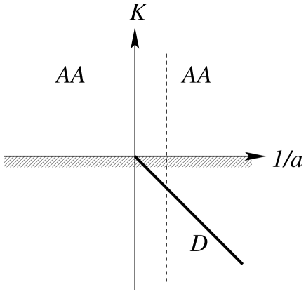
Figure 1: The $a^{-1}$–$K$ plane for the 2-body problem. The allowed region for atom-atom scattering states are the two quadrants labelled $AA$. The heavy line labelled $D$ is the shallow dimer. The cross-hatching indicates the 2-atom threshold.

The $a^{-1}$–$K$ plane for the 2-body system in the scaling limit is shown in Fig. 1. The possible states are atom-atom scattering states ($AA$) and the shallow dimer ($D$). The threshold for atom-atom scattering states is indicated by the hatched area. The shallow dimer is represented by the heavy line given by the ray $\xi=-{1\over 4}\pi$. A given physical system has a specific value of the scattering length, and so is represented by a vertical line, such as the dashed line in Fig. 1. Changing $a$ corresponds to sweeping the line horizontally across the page. The resonant limit corresponds to tuning the vertical line to the $K$ axis.

3.4 Scaling violations

The continuous scaling symmetry is a trivial consequence of the fact that $a$ is the only length scale that remains nonzero in the scaling limit. For real atoms, the scaling limit can only be an approximation. There are scaling violations that give corrections that are suppressed by powers of $\ell/|a|$. In the 2-body sector, the most important scaling violations come from the S-wave effective range $r_{s}$ defined by the effective-range expansion in Eq. (5).

The differential cross section for atom-atom scattering can be expanded in powers of $\ell/a$ with $ak$ fixed:

$${d\sigma\over d\Omega} = {4a^{2}\over 1+a^{2}k^{2}}\left(1+{r_{s}\over a}\,{a^{2}k^{2}\over 1+a^{2}k^{2}}+\ldots\right)\,.$$ (33)

The leading term is the universal expression in Eq. (24). The next-to-leading term is determined by $r_{s}$.

If $a>0$, we can also consider the scaling violations to the binding energy of the shallow dimer. The binding energy can be expanded in powers of $\ell/a$:

$$E_{2}^{(-)}\approx{\hbar^{2}\over ma^{2}}\left(1+{r_{s}\over a}+{5r_{s}^{2}\over 4a^{2}}+\ldots\right)\,.$$ (34)

The leading term is the universal expression in Eq. (27). The first two correction terms are determined by $r_{s}$.

4 Three Identical Bosons

In this section, we summarize the universal properties of three identical bosons in the scaling limit in which the only scales are those provided by the large scattering length $a$ and the Efimov parameter $\kappa_{*}$.

4.1 Boundary condition at short distances

When the scattering length is large compared to the natural low-energy length scale $\ell$, the range of the hyperradius $R$ includes four important regions. It is useful to give names to each of these regions:

• the short-distance region $R\hskip 1.99997pt\raisebox{2.15277pt}{$<$}\raisebox{-3.00003pt}{$\sim$}\hskip 1.99997pt|\ell|$,

• the scale-invariant region $\ell\ll R\ll|a|$,

• the long-distance region $R\sim|a|$,

• the asymptotic region $R\gg|a|$.

In the scaling limit $\ell\to 0$, the short-distance region shrinks to 0. Its effects can however be taken into account through a boundary condition on the hyperradial wavefunction in the scale-invariant region.

The hyperspherical expansion of the Faddeev wave function is given in Eq. (20). In the scaling limit, the channel eigenvalues $\lambda_{n}(R)$ determined by the eigenvalue equation for the hyperangular functions $\phi_{n}(R,\alpha)$ satisfy [2]

$$\cos\left(\lambda^{1/2}\mbox{$\pi\over 2$}\right)-{8\over\sqrt{3}}\lambda^{-1/2}\sin\left(\lambda^{1/2}\mbox{$\pi\over 6$}\right)=\sqrt{2}\lambda^{-1/2}\sin\left(\lambda^{1/2}\mbox{$\pi\over 2$}\right){R\over a}\,.$$ (35)

The lowest channel potentials $V_{n}(R)$ defined by Eq. (21) are shown in Fig. 2.

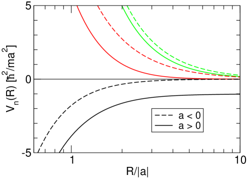
Figure 2: The three lowest hyperspherical potentials $V_{n}(R)$ scaled by $\hbar^{2}/ma^{2}$ for $a>0$ (solid lines) and for $a<0$ (dashed lines).

For $R\ll|a|$, the channel eigenvalues approach constants $\lambda_{n}(0)$ and the channel potentials in Eq. (21) have the scale-invariant behavior $1/R^{2}$. Whether $a$ is positive or negative, the lowest eigenvalue $\lambda_{0}(R)$ is negative at $R=0$. It can be expressed as $\lambda_{0}(0)=-s_{0}^{2}$, where $s_{0}\approx 1.00624$ is the solution to the transcendental equation

$$s_{0}\cosh{\pi s_{0}\over 2}={8\over\sqrt{3}}\sinh{\pi s_{0}\over 6}\,.$$ (36)

Thus the potential $V_{0}(R)$ is an attractive $1/R^{2}$ potential for $R\ll|a|$:

$$V_{0}(R)\approx-(4+s_{0}^{2}){\hbar^{2}\over 2mR^{2}},\hskip 28.45274pt\ell\ll R\ll|a|\,.$$ (37)

All the channel eigenvalues for $n\geq 1$ are positive at $R=0$: $\lambda_{n}(0)\geq 19.94$. Thus all the channel potentials $V_{n}(R)$ for $n\geq 1$ are repulsive $1/R^{2}$ potentials in the region $R\ll|a|$. The hyperradial wave functions $f_{n}(R)$ for $n\geq 1$ therefore decrease exponentially for $R\ll|a|$.

In the scaling limit $\ell\to 0$, the lowest adiabatic hypersherical potential in Eq. (37) behaves like $1/R^{2}$ all the way down to $R=0$. Such a potential is too singular to have well-behaved solutions. If the exact solution $f(R)$ for the hyperradial wave function at short distances was known, it could be matched onto the solution in the scaling limit by choosing a hyperradius $R_{0}$ in the scale-invariant region and demanding that the logarithmic derivatives $R_{0}f^{\prime}(R_{0})/f(R_{0})$ match at that point. If we also choose $R_{0}\ll(m|E|/\hbar^{2})^{-1/2}$, the energy eigenvalue $E$ in Eq. (22) can be neglected relative to the channel potential. The most general solution for the hyperradial wave function in the scale-invariant region is

$$f(R)=R^{1/2}\left[Ae^{is_{0}\ln(HR)}+Be^{-is_{0}\ln(HR)}\right]\,,$$ (38)

where $A$ and $B$ are arbitrary coefficients. To make the arguments of the logarithms dimensionless, we have inserted factors of $H$, the wavenumber variable defined in Eq. (32). The terms with the coefficients $A$ and $B$ represent an outgoing hyperradial wave and an incoming hyperradial wave, respectively. If $|A|<|B|$, there is a net flow of probability into the short-distance region. As will be discussed in detail in Section 5, such a flow of probability is possible if there are deep diatomic molecules. In this section, we assume that there are no deep 2-body bound states. The probability in the incoming hyperradial wave must therefore be totally reflected at short distances. This requires $|A|=|B|$, which implies that $A$ and $B$ differ only by a phase:

$$A=-e^{2i\theta_{*}}B$$ (39)

for some angle $\theta_{*}$. This angle can be expressed as $\theta_{*}=-s_{0}\ln(H/\Lambda_{0})$, where $\Lambda_{0}$ is the product of $1/R_{0}$ and a complicated function of $R_{0}f^{\prime}(R_{0})/f(R_{0})$. The effects of the short-distance region on $f(R)$ enter only through the wavenumber variable $\Lambda_{0}$. By solving the hyperradial equation for the scale-invariant potential in Eq. (37), we find that $\Lambda_{0}$ differs from the 3-body parameter $\kappa_{*}$ defined by the Efimov spectrum in the resonant limit only by a multiplicative numerical constant. Thus the angle $\theta_{*}$ in Eq. (39) can be expressed as

$$\theta_{*}=-s_{0}\ln(cH/\kappa_{*})\,,$$ (40)

where $H$ is defined in Eq. (32) and $c$ is a constant.

4.2 Discrete scaling symmetry

The boundary condition in Eq. (39) gives logarithmic scaling violations that give corrections to the scaling limit that are functions of $\ln(H/\kappa_{*})$. Logarithmic scaling violations do not become less important as one approaches the scaling limit, and therefore cannot be treated as perturbations. Because the boundary condition enters through the phase in Eq. (39), the logarithmic scaling violations must be log-periodic functions of $H/\kappa_{*}$ with period $\pi/s_{0}$.

The 3-body sector in the scaling limit has a trivial continuous scaling symmetry defined by Eqs. (29) together with $\kappa_{*}\to\lambda^{-1}\kappa_{*}$. However, because of the log-periodic form of the logarithmic scaling violations, it also has a nontrivial discrete scaling symmetry. There is a discrete subgroup of the continuous scaling symmetry that remains an exact symmetry in the scaling limit:

$$\kappa_{*} \longrightarrow \kappa_{*}\,,\qquad a\longrightarrow\lambda_{0}^{n}a\,,\qquad{\bm{r}}\longrightarrow\lambda_{0}^{n}{\bm{r}}\,,\qquad t\longrightarrow\lambda_{0}^{2n}t\,,$$ (41)

where $n$ is an integer, $\lambda_{0}=e^{\pi/s_{0}}$, and $s_{0}\approx 1.00624$ is the solution to the transcendental equation in Eq. (36). The numerical value of the discrete scaling factor is $e^{\pi/s_{0}}\approx 22.7$. Under the discrete scaling symmetry, 3-body observables, such as binding energies and cross sections, scale with the integer powers of $\lambda_{0}$ suggested by dimensional analysis. By combining the trivial continuous scaling symmetry with the discrete scaling symmetry given by Eqs. (41), we can see that $\kappa_{*}$ is only defined modulo multiplicative factors of $\lambda_{0}$.

The discrete scaling symmetry strongly constrains the dependence of the observables on the parameters $a$ and $\kappa_{*}$ and on kinematic variables. For example, the scaling of the atom-dimer cross section is $\sigma_{AD}\to(\lambda_{0}^{m})^{2}\sigma_{AD}$. The discrete scaling symmetry constrains its dependence on $a$, $\kappa_{*}$, and the energy $E$:

$$\sigma_{AD}(\lambda_{0}^{-2m}E;\lambda_{0}^{m}a,\kappa_{*})=\lambda_{0}^{2m}\sigma_{AD}(E;a,\kappa_{*})\,,$$ (42)

for all integers $m$. At $E=0$, the cross section is simply $\sigma_{AD}=4\pi|a_{AD}|^{2}$, where $a_{AD}$ is the atom-dimer scattering length. The constraint in Eq. (42) implies that the atom-dimer scattering length $a_{AD}$ is proportional to $a$ with a coefficient that is a log-periodic function of $a\kappa_{*}$ with period $\pi/s_{0}$. The explicit expression for the atom-dimer scattering length is given in Eq. (61) and it is indeed consistent with this constraint.

To illustrate the discrete scaling symmetry, it is convenient to use the interaction variable $1/a$ and the energy variable $K$ defined in Eq. (31). For a given value of $\kappa_{*}$, the set of all possible low-energy 3-body states in the scaling limit can be represented as points $(a^{-1},K)$ on the plane whose horizontal axis is $1/a$ and whose vertical axis is $K$. The discrete scaling transformation in Eqs. (41) is simply a rescaling of the radial variable $H$ defined in Eq. (32) with $\kappa_{*}$ and $\xi$ fixed: $H\to\lambda_{0}^{-m}H$.

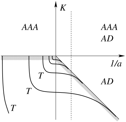
Figure 3: The $a^{-1}$–$K$ plane for the 3-body problem. The allowed regions for 3-atom scattering states and for atom-dimer scattering states are labelled $AAA$ and $AD$, respectively. The heavy lines labeled $T$ are three of the infinitely many branches of Efimov states. The cross-hatching indicates the threshold for scattering states.

The $a^{-1}$–$K$ plane for three identical bosons in the scaling limit is shown in Fig. 3. The possible states are 3-atom scattering states ($AAA$), atom-dimer scattering states ($AD$), and Efimov trimers ($T$). The threshold for scattering states is indicated by the hatched area. The Efimov trimers are represented by the heavy lines below the threshold. There are infinitely many branches of Efimov trimers, but only a few are shown. They intercept the vertical axis at the points $K=-(e^{-\pi/s_{0}})^{n-n_{*}}\kappa_{*}$. A given physical system has a specific value of the scattering length, and so is represented by a vertical line. The resonant limit corresponds to tuning the vertical line to the $K$ axis.

Figure 4: The energy variable $K$ for the branch of Efimov trimers labelled by $n=n_{*}$ as a function of $1/a$. In the resonant limit, the binding wave number is $\kappa_{*}$. The branch disappears through the atom-dimer threshold at $a=a_{*}$ and through the 3-atom threshold at $a=a_{*}^{\prime}$.

Changing $1/a$ continuously from a large positive value to a large negative value corresponds to sweeping the vertical dashed line in Fig. 3 from right to left across the page. The Efimov trimers appear one by one at the atom-dimer threshold at positive critical values of $1/a$ that differ by powers of $e^{\pi/s_{0}}\approx 22.7$ until there are infinitely many at $1/a=0$. As $1/a$ continues to decrease through negative values, the Efimov trimers disappear one by one through the 3-atom threshold at negative critical values of $1/a$ that differ by powers of $e^{\pi/s_{0}}$. We will focus on the specific branch of Efimov trimers labelled by the integer $n=n_{*}$, which is illustrated in Fig. 4. At some positive critical value $a=a_{*}$, this branch of Efimov trimers appears at the atom-dimer threshold: $E_{T}^{(n_{*})}=E_{D}$. As $a$ increases, its binding energy $E_{T}^{(n_{*})}-E_{D}$ relative to the atom-dimer threshold increases but its binding energy $E_{T}^{(n_{*})}$ relative to the 3-atom threshold decreases monotonically. As $a\to\infty$, the binding energy approaches a nontrivial limit: $E_{T}^{(n_{*})}\to\hbar^{2}\kappa_{*}^{2}/m$. For $a<0$, as $|a|$ decreases, $E_{T}^{(n_{*})}$ continues to decrease monotonically. Finally, at some negative critical value $a=a_{*}^{\prime}$, it disappears through the 3-atom threshold.

4.3 Efimov trimers

The binding energies of the Efimov states are functions of $a$ and $\kappa_{*}$. Efimov showed that the calculation of the binding energies for all the Efimov states could be reduced to the calculation of a single universal function of $\xi$. The Efimov states can be interpreted as bound states in the lowest adiabatic hyperspherical potential. This potential has a scale-invariant region where the general solution is the sum of an outgoing hyperradial wave and an incoming hyperradial wave as in Eq. (38). Bound states occur at energies for which the wave reflected from the long-distance region $R\sim|a|$ come into resonance with the wave reflected from the short-distance region $R\sim\ell$. The resonance condition can be expressed as

$$2\theta_{*}+\Delta(\xi)=0\mod 2\pi\,,$$ (43)

where $\Delta(\xi)/2$ is the phase shift of a hyperradial wave that is reflected from the long-distance region. Using the expression for $\theta_{*}$ in Eq. (40) and the definitions for $H$ and $\xi$ in Eq. (32), we obtain Efimov’s equation for the binding energies:

$$E_{T}+{\hbar^{2}\over ma^{2}}=\left(e^{-2\pi/s_{0}}\right)^{n-n_{*}}\exp\left[\Delta(\xi)/s_{0}\right]\frac{\hbar^{2}\kappa_{*}^{2}}{m}\,,$$ (44)

where the angle $\xi$ is defined by

$$\tan\xi=-(mE_{T}/\hbar^{2})^{1/2}\,a\,.$$ (45)

We have absorbed the constant $c$ in Eq. (40) into the function $\Delta(\xi)$ so that it satisfies $\Delta(-{1\over 2}\pi)=0$.

Once the universal function $\Delta(\xi)$ has been calculated, the binding energies for all the Efimov states for any values of $a$ and $\kappa_{*}$ can be obtained by solving Eq. (44). The equation is the same for different Efimov states except for the factor of $(e^{-2\pi/s_{0}})^{n}$ on the right side.

Efimov’s universal function $\Delta(\xi)$ was calculated in Ref. [24] with a few digits of precision over the entire range $-\pi<\xi<-{1\over 4}\pi$. It has been calculated in Ref. [25] with a precision of about 12 digits for $a>0$, which corresponds to the range $-{1\over 2}\pi<\xi<-{1\over 4}\pi$. It decreases from 6.0273 at $\xi=-{1\over 4}\pi$ to 0 at $\xi=-{1\over 2}\pi$ and then to about $-0.89$ at $\xi=-\pi$. A parameterization of $\Delta(\xi)$ is given in Ref. [6] that has errors less than about 0.01, at least in the range $-{1\over 2}\pi<\xi<-{1\over 4}\pi$.

In the resonant limit $a\to\pm\infty$, the spectrum $E_{T}^{(n)}$ of the Efimov states is particularly simple. In this limit, $\xi\to-{1\over 2}\pi$ and $\Delta(\xi)\to 0$, so the solutions to Eq. (44) reduce to

$$E_{T}^{(n)}=\left(e^{-2\pi/s_{0}}\right)^{n-n_{*}}{\hbar^{2}\kappa_{*}^{2}\over m}\,,\hskip 28.45274pta=\pm\infty,$$ (46)

where $\kappa_{*}$ is the binding wave number for the Efimov state labeled by $n=n_{*}$. The spectrum in Eq. (46) is geometric, with the binding energies of successive Efimov states having the ratio $e^{-2\pi/s_{0}}\approx 1/515.03$. The Schrödinger wave function in the center-of-mass frame for an Efimov state with binding energy $E_{T}=\hbar^{2}\kappa^{2}/m$ is

$$\Psi({\bm{r}}_{1},{\bm{r}}_{2},{\bm{r}}_{3})=R^{-5/2}f_{0}(R)\sum_{i=1}^{3}{\sinh\left[s_{0}({\pi\over 2}-\alpha_{i})\right]\over\sin(2\alpha_{i})}\,.$$ (47)

The hyperradial wavefunction is

$$f_{0}(R)=R^{1/2}K_{is_{0}}(\sqrt{2}\kappa R)\,,$$ (48)

where $K_{is_{0}}(z)$ is a Bessel function with imaginary index. A quantitative measure of the size of a 3-body bound state is the mean-square hyperradius:

$$\langle R^{2}\rangle^{(n)}=\left(e^{2\pi/s_{0}}\right)^{n-n_{*}}{2(1+s_{0}^{2})\over 3}\kappa_{*}^{-2}\,.$$ (49)

Thus the root-mean-square hyperradius for each successively shallower Efimov state is larger than the previous one by $e^{\pi/s_{0}}\approx 22.7$.

The Efimov trimers disappear through the atom-dimer threshold at positive critical values of $a$, as illustrated in Fig. 4. For the branch of Efimov trimers labelled by $n=n_{*}$, the critical value is

$$a_{*}=0.0707645086901\,\kappa_{*}^{-1}\,.$$ (50)

The other critical values are $(e^{\pi/s_{0}})^{n}a_{*}$, where $n$ is an integer. The binding energy $E_{T}^{(N)}$ for the Efimov state just below the atom-dimer threshold is

$$E_{T}^{(N)}\approx E_{D}\big{[}1+0.164\,\ln^{2}(a/a_{*})\big{]}\,.$$ (51)

The errors in this approximation scale as $(a-a_{*})^{3}$.

Efimov states near the atom-dimer threshold can be understood intuitively as 2-body systems composed of an atom of mass $m$ and a dimer of mass $2m$. We can exploit the universality of the 2-body systems with large scattering lengths to deduce some properties of the shallowest Efimov state when it is close to the atom-dimer threshold. The analog of the universal formula in Eq. (27) is obtained by replacing the reduced mass $m/2$ of the atoms by the reduced mass $2m/3$ of the atom and dimer and by repacing $a$ by the atom-dimer scattering length $a_{AD}$ which diverges at $a=a_{*}$. Thus the binding energy relative to the 3-atom threshold can be approximated by

$$E_{T}^{(N)}\approx E_{D}+{3\hbar^{2}\over 4ma_{AD}^{2}}\,.$$ (52)

An explicit expression for the atom-dimer scattering length $a_{AD}$ is given in Eq. (61). The binding energy in Eq. (52) agrees with the result in Eq. (51) up to errors of order $a/a_{AD}^{3}$, which scales as $(a-a_{*})^{3}$. We can also use universality to deduce the wave function of the Efimov trimer. The Schrödinger wave function can be expressed as the sum of three Faddeev wave functions as in Eq. (19). In the limit $r_{1,23}\gg r_{23}$, the first Faddeev wave function should have the form

$$\psi^{(1)}({\bm{r}}_{23},{\bm{r}}_{1,23})\approx\psi_{AD}(r_{1,23})\,\psi_{D}(r_{23})\,,$$ (53)

where $\psi_{D}(r)$ is the dimer wave function given in Eq. (28) and $\psi_{AD}(r)$ is the analogous universal wave function for a shallow bound state consisting of two particles with large positive scattering length $a_{AD}$:

$$\psi_{AD}(r)={1\over r}e^{-r/a_{AD}}\,.$$ (54)

This Faddeev wave function can be expressed in terms of hyperspherical coordinates using Eqs. (13) and (14). Most of the support of the probability density $|\Psi|^{2}$ is concentrated in the region in which the hyperradius is very large, $R\sim a_{AD}$, and one of the three hyperangles is very small, $\alpha_{i}\ll 1$. The mean-square hyperradius can be calculated easily when $a_{AD}\gg a$:

$$\langle R^{2}\rangle^{(N)}\approx\mbox{$1\over 3$}a_{AD}^{2}\,.$$ (55)

This result can be obtained more easily simply by using the universal atom-dimer wave function in Eq. (54) and the approximate expression $R^{2}\approx{2\over 3}r^{2}$ for the hyperradius.

The Efimov trimers disappear through the 3-atom threshold at negative critical values of $a$, as illustrated in Fig. 4. For the branch of Efimov trimers labelled by $n=n_{*}$, the critical value is

$$a_{*}^{\prime}=-1.56(5)\,\kappa_{*}^{-1}\,.$$ (56)

The other critical values are $(e^{\pi/s_{0}})^{n}a_{*}^{\prime}$, where $n$ is an integer. In contrast to $a_{*}$ in Eq. (50), only a few of digits of precision are currently available for $a_{*}^{\prime}$. Comparing Eqs. (50) and (56), we see that $a_{*}^{\prime}\approx-22.0\;a_{*}$.

There is an Efimov trimer at the 3-atom threshold when $a$ has the negative critical value $a_{*}^{\prime}$. As can be seen in Fig. 4, the binding energy $E_{T}^{(n)}$ of the Efimov trimer increases rapidly as a function of $a$ when $|a|$ exceeds $|a_{*}^{\prime}|$. The increase is so rapid that in Ref. [24], a parameterization of the universal function $\Delta(\xi)$ in Eq. (44) with an essential singularity at $a=a_{*}^{\prime}$ was used to get a good fit to the binding energy. The result of Refs. [26] and [27] seem to indicate that $E_{T}^{(n)}$ is actually linear in $1/a$ near $a=a_{*}^{\prime}$ with a large slope. The results of a calculation in Ref. [27] can be used to obtain the approximation

$$E_{T}^{(n)}=\left(1.1\,\ln{a\over a_{*}^{\prime}}\right){\hbar^{2}\over ma^{2}}\,.$$ (57)

When $|a|$ decreases below $|a_{*}^{\prime}|$, the Efimov trimer does not immediately disappear, but instead becomes a resonance that decays into three atoms. This resonance is associated with a pole at a complex energy $E_{\rm res}-i\Gamma_{\rm res}/2$ with a positive real part and a negative imaginary part. This complex energy is the analytic continuation of the energy $-E_{T}^{(n)}$ of the shallowest Efimov trimer for $|a|<|a_{*}^{\prime}|$. For $a$ close to $a_{*}^{\prime}$, the real part of the resonance energy is given simply by the negative of the expression in Eq. (57). The authors of Ref. [27] gave a parameterization of the imaginary part of the resonance energy that scales as $(a-a_{*}^{\prime})^{2}$ near the threshold. However their numerical results seem to suggest that $\Gamma_{\rm res}$ scales as a higher power of $a-a_{*}^{\prime}$.

There is a common misconception in the literature that Efimov states must have binding energies that differ by multiplicative factors of 515.03. However, this ratio applies only in the resonant limit $a\to\pm\infty$. The ratio $E_{T}^{(n-1)}/E_{T}^{(n)}$ of the binding energies of adjacent Efimov trimers can be much smaller than 515 if $a>0$ and much larger than 515 if $a<0$. The smallest ratios occur at the critical values $(e^{\pi/s_{0}})^{n}a_{*}$, where $a_{*}$ is given in Eq. (50). The accurate results of Ref. [25] for the binding energies $E_{T}$ of the first few Efimov states in units of $E_{D}=\hbar^{2}/ma^{2}$ are

$$E_{T}^{(N)}\hskip 8.5359pt = E_{D}\,,$$ (58a)

$$E_{T}^{(N-1)} = 6.75029015026\,E_{D}\,,$$ (58b)

$$E_{T}^{(N-2)} = 1406.13039320\,E_{D}\,.$$ (58c)

Thus, if $a>0$, the ratio $E_{T}^{(N-1)}/E_{T}^{(N)}$ of the binding energies for the two shallowest Efimov trimers can range from about 6.75 to about 208. The largest ratios occur at the critical values $(e^{\pi/s_{0}})^{n}a_{*}^{\prime}$, where $a_{*}^{\prime}$ is given in Eq. (56). The binding energies $E_{T}$ of the first few Efimov states are [24]

$$E_{T}^{(N)}\hskip 8.5359pt = 0\,,$$ (59a)

$$E_{T}^{(N-1)} = 1.09\times 10^{3}\;\hbar^{2}/ma^{2}\,,$$ (59b)

$$E_{T}^{(N-2)} = 5.97\times 10^{5}\;\hbar^{2}/ma^{2}\,.$$ (59c)

Thus, if $a<0$, the ratio $E_{T}^{(N-1)}/E_{T}^{(N)}$ of the binding energies for the two shallowest Efimov states can range from about 550 to $\infty$.

4.4 Atom-dimer elastic scattering

The differential cross section for elastic atom-dimer scattering near the atom-dimer threshold can be expressed in terms of the atom-dimer scattering length $a_{AD}$:

$${d\sigma_{AD}\over d\Omega}\longrightarrow|a_{AD}|^{2}\,,\qquad{\rm as\ }E\to-E_{D}\,.$$ (60)

The discrete scaling symmetry implies that $a_{AD}/a$ must be a log-periodic function of $a\kappa_{*}$ with period $\pi/s_{0}$. Its functional form was deduced by Efimov up to a few numerical constants. The numerical constants were first calculated in Ref. [28]. The atom-dimer scattering length is

$$a_{AD}=\big{(}1.46+2.15\cot[s_{0}\ln(a/a_{*})]\big{)}\;a\,,$$ (61)

where $a_{*}\approx 0.071\,\kappa_{*}^{-1}$ is given to high precision in Eq. (50). The atom-dimer scattering length diverges if $a$ has one of the values $(e^{\pi/s_{0}})^{n}a_{*}$ for which there is an Efimov state at the atom-dimer threshold. It vanishes if $a$ has one of the values $(e^{\pi/s_{0}})^{n}\,0.38\,a_{*}$.

4.5 Three-body recombination

Three-body recombination is a process in which three atoms collide to form a diatomic molecule and an atom. The energy released by the binding energy of the molecule goes into the kinetic energies of the molecule and the recoiling atom. The 3-body recombination rate depends on the momenta of the three incoming atoms. If their momenta are sufficiently small compared to $1/|a|$, the dependence on the momenta can be neglected, and the recombination rate reduces to a constant. The recombination event rate constant $\alpha$ is defined such that the number of recombination events per time and per volume in a gas of cold atoms with number density $n_{A}$ is $\alpha n^{3}_{A}$. If the atom and the dimer produced by the recombination process have large enough kinetic energies to escape from the system, the rate of decrease in the number density of atoms is

$${d\ \over dt}n_{A} = -3\alpha n^{3}_{A}\,,$$ (62)

In a Bose-Einstein condensate, the three atoms must all be in the same quantum state, so the coefficient of $n_{A}^{3}$ in Eq. (62) must be multiplied by 1/3! to account for the symmetrization of the wave functions of the three identical particles [29]. This prediction was first tested by the JILA group [30]. They measured the 3-body loss rates in an ultracold gas of ⁸⁷Rb atoms in the $|f,m_{f}\rangle=|1,-1\rangle$ hyperfine state, both above and below the critical temperature for Bose-Einstein condensation. They found that the loss rate was smaller in the Bose-Einstein condensate by a factor of $7.4(2.6)$, in agreement with the predicted value of 6 [29].

If the scattering length $a$ is negative, the molecule can only be a deep diatomic molecule with binding energy of order $\hbar^{2}/m\ell^{2}$ or larger. However, if $a$ is positive and unnaturally large ($a\gg\ell$), the molecule can also be the shallow dimer with binding energy $E_{D}=\hbar^{2}/ma^{2}$. Three-body recombination into deep dimers will be discussed in Section 5. In this section, we assume there are no deep dimers. We therefore assume $a>0$ and focus on 3-body recombination into the shallow dimer. We denote the contribution to the rate constant $\alpha$ from 3-body recombination into the shallow dimer by $\alpha_{\rm shallow}$.

Dimensional analysis together with the discrete scaling symmetry implies that $\alpha_{\rm shallow}$ is proportional to $\hbar a^{4}/m$ with a coefficient that is a log-periodic function of $a\kappa_{*}$ with period $\pi/s_{0}$. An analytic expression for $\alpha_{\rm shallow}$ has recently been derived [31, 32]:

$$\alpha_{\rm shallow}={128\pi^{2}(4\pi-3\sqrt{3})\sin^{2}[s_{0}\ln(a/a_{*0})]\over\sinh^{2}(\pi s_{0})+\cos^{2}[s_{0}\ln(a/a_{*0})]}\,{\hbar a^{4}\over m}\,,$$ (63)

where $a_{*0}$ differs from $\kappa_{*}^{-1}$ by a multiplicative constant that is known only to a couple of digits of accuracy:

$$a_{*0}\approx 4.5\,a_{*}\approx 0.32\,\kappa_{*}^{-1}\,.$$ (64)

The maximum value of the coefficient of $\hbar a^{4}/m$ in Eq. (63) is

$$C_{\rm max}={128\pi^{2}(4\pi-3\sqrt{3})\over\sinh^{2}(\pi s_{0})}\,.$$ (65)

Its numerical value is $C_{\rm max}=67.1177$. We can exploit the fact that $\sinh^{2}(\pi s_{0})\approx 139$ is large to simplify the expression in Eq. (63). The rate constant can be approximated with an error of less than 1% of $C_{\rm max}\hbar a^{4}/m$ by

$$\alpha_{\rm shallow}\approx 67.12\sin^{2}[s_{0}\ln(a/a_{*0})]\,\hbar a^{4}/m\,.$$ (66)

This approximate functional form of the rate constant was first deduced in Refs. [33, 34]. The coefficient $C_{\rm max}$ and the relation between $a_{*0}$ and $\kappa_{*}$ was calculated accurately in Refs. [35, 36].

The most remarkable feature of the analytic expression in Eq. (63) and the approximate expression in Eq. (66) is that the coefficient of $\hbar a^{4}/m$ oscillates between zero and 67.12 as a function of $\ln(a)$. In particular, $\alpha_{\rm shallow}$ has zeroes at values of $a$ given by $(e^{\pi/s_{0}})^{n}\,a_{*0}$, where $a_{*0}\approx 4.5\,a_{*}$. The maxima of $\alpha_{\rm shallow}$ in Eq. (66) occur at the values of $a$ for which $\tan[s_{0}\ln(a/a_{*0})]=-s_{0}/2$, which are $a\approx(e^{\pi/s_{0}})^{n}\,64.3\,a_{*}\approx(e^{\pi/s_{0}})^{n}4.6\,\kappa_{*}^{-1}$.

Since the zeroes in $\alpha_{\rm shallow}$ are so remarkable, it is worth enumerating the effects that will tend to fill in the zeroes, turning them into local minima of $\alpha_{\rm shallow}$. The zeroes arise from the interference between two pathways associated with the lowest two adiabatic hyperspherical channels. There may be additional contributions from coupling to higher hyperspherical channels, but in the scaling limit they are strongly suppressed numerically. The zero in $\alpha_{\rm shallow}$ for $a=a_{*0}$ is exact only at threshold. If the recombining atoms have collision energy $E$, $\alpha_{\rm shallow}$ goes to zero as $E^{2}$ as $E\rightarrow 0$ [37]. Thus thermal effects that give nonzero collision energy to the atoms will tend to fill in the zeroes. Finally, if the 2-body potential supports deep diatomic molecules, their effects will tend to fill in the zeros of $\alpha_{\rm shallow}$ as described in Section 5.4. Furthermore, as described in Section 5.4, 3-body recombination into those deep dimers gives an additional nonzero contribution $\alpha_{\rm deep}$ to the rate constant $\alpha$.

5 Effects of Deep Diatomic Molecules

In this Section, we describe the effects of deep diatomic molecules on the universal properties for three identical bosons in the scaling limit.

5.1 Boundary condition at short distances

The existence of deep dimers requires a modification of the boundary condition on the hyperradial wave function at short distances. The general solution for the hyperradial wave function in the lowest hyperspherical potential in the scale-invariant region $\ell\ll R\ll|a|$ is given in Eq. (38). The boundary condition in Eq. (39), which takes into account the effects of short distances $R\hskip 1.99997pt\raisebox{2.15277pt}{$<$}\raisebox{-3.00003pt}{$\sim$}\hskip 1.99997pt\ell$, follows from the assumption that all the probability in an incoming hyperradial wave is reflected back from the short-distance region into an outgoing hyperradial wave. If there are deep dimers, some of the probability in the incoming hyperradial wave that flows into the short-distance region emerges in the form of scattering states that consist of an atom and a deep dimer with large kinetic energy but small total energy. We will refer to these states as high-energy atom-dimer scattering states.

The 2-body potentials for the alkali atoms other than hydrogen support diatomic molecules with many vibrational energy levels. If it was necessary to take into account each of these deep dimers explicitly, the problem would be extremely difficult. Fortunately the cumulative effect of all the deep dimers on low-energy 3-atom observables can be taken into account through one additional parameter: an inelasticity parameter $\eta_{*}$ that determines the widths of the Efimov trimers. In the scaling limit, the low-energy 3-body observables are completely determined by $a$, $\kappa_{*}$, and $\eta_{*}$.

The reason the cumulative effects of the deep dimers can be described by a single number $\eta_{*}$ is that all pathways from a low-energy 3-atom state to a high-energy atom-dimer scattering state must flow through the lowest hyperspherical potential, which in the scale-invariant region has the form given in Eq. (37). The reason for this is that in order to reach a high-energy atom-dimer scattering state, the system must pass through an intermediate configuration in which all three atoms are simultaneously close together with a hyperradius $R$ of order $\ell$ or smaller. Such small values of $R$ are accessible to a low-energy 3-atom state only through the lowest hyperspherical potential.

If there are deep dimers, some of the probability in a hyperradial wave that flows to short distances emerges in the form of high-energy atom-dimer scattering states. We denote the fraction of the probability that is reflected back to long distances by $e^{-4\eta_{*}}$. We refer to $\eta_{*}$ as the Efimov width parameter. The amplitude $A$ of the outgoing wave in Eq. (38) then differs from the amplitude $B$ of the incoming wave not only by a phase as in Eq. (39) but also by a suppression factor $e^{-2\eta_{*}}$. Thus if there are deep 2-body bound states, the boundary condition in Eq. (39) must be replaced by

$$A=-e^{-2\eta_{*}+2i\theta_{*}}B.$$ (67)

The angle $\theta_{*}$ is related to the 3-body parameter $\kappa_{*}$ by Eq. (40). The parameters $\kappa_{*}$ and $\eta_{*}$ appear in the boundary condition in Eq. (67) in the combination $\theta_{*}+i\eta_{*}$. If the universal results for the case $\eta_{*}=0$ can be expressed as an analytic function of $\ln(\kappa_{*})$, then the corresponding universal results for the case in which there are deep 2-body bound states can be obtained simply by the substitution $\ln(\kappa_{*})\to\ln(\kappa_{*})+i\eta_{*}/s_{0}$.

One can also obtain universal results for the total probability of transitions from low-energy 3-atom or atom-dimer scattering states to high-energy atom-dimer scattering states. The transition rate for any individual deep dimer is sensitive to the details of wave functions in the short-distance region $R\sim\ell$. However the inclusive rate summed over all deep dimers is much less sensitive to short distances, because it is constrained by probability conservation. The inclusive rates are given by universal expressions that include a factor of $1-e^{-4\eta_{*}}$ [38], which is the probability that a hyperradial wave is not reflected from the short-distance region.

5.2 Widths of Efimov states

One obvious consequence of the existence of deep dimers is that the Efimov trimers are no longer sharp states. They are resonances with nonzero widths, because they can decay into an atom and a deep dimer. The binding energy $E_{T}$ and width $\Gamma_{T}$ of an Efimov resonance can be obtained as a complex eigenvalue $E=-(E_{T}+i\Gamma_{T}/2)$ of the 3-body Schrödinger equation.

In the absence of deep dimers, the binding energies of Efimov trimers satisfy Eq. (44), where $\Delta(\xi)/2$ is the phase shift of a hyperradial wave that is reflected from the long-distance region $R\sim|a|$. To obtain the corresponding equation in the case of deep dimers, we need only make the substitution $\theta_{*}\to\theta_{*}+i\eta_{*}$ in Eq. (43):

$$2(\theta_{*}+i\eta_{*})+\Delta(\xi)=0\mod 2\pi.$$ (68)

This can be satisfied only if we allow complex values of $\xi$ in the argument of $\Delta$. Using the expression for $\theta_{*}$ in Eq. (40) and inserting the definition of $H$ in Eq. (32), we obtain the equation

$$E_{T}+{i\over 2}\Gamma_{T}+{\hbar^{2}\over ma^{2}} = \left(e^{-2\pi/s_{0}}\right)^{n-n_{*}}\exp\left[{\Delta(\xi)+2i\eta_{*}\over s_{0}}\right]{\hbar^{2}\kappa_{*}^{2}\over m}\,,$$ (69)

where the complex-valued angle $\xi$ is defined by

$$\tan\xi=-\big{(}m(E_{T}+i\Gamma_{T}/2)/\hbar^{2}\big{)}^{1/2}\,a\,.$$ (70)

To solve this equation for $E_{T}$ and $\Gamma_{T}$, we need the analytic continuation of $\Delta(\xi)$ to complex values of $\xi$. The parametrization for $\Delta(\xi)$ in Ref. [6] should be accurate for complex values of $\xi$ with sufficiently small imaginary parts, except near $\xi=-\pi$ where the parametrization used an expansion parameter that was not based on any analytic understanding of the behavior near the endpoint. If the analytic continuation of $\Delta(\xi)$ were known, the binding energy and width of one Efimov state could be used to determine $\kappa_{*}$ and $\eta_{*}$. The remaining Efimov states and their widths could then be calculated by solving Eq. (69).

If the Efimov width parameter $\eta_{*}$ is extremely small, the right side of Eq. (69) can be expanded to first order in $\eta_{*}$. The resulting expression for the width is

$$\Gamma_{T}\approx{4\eta_{*}\over s_{0}}\left(E_{T}+{\hbar^{2}\over ma^{2}}\right)\,.$$ (71)

For the shallowest Efimov states, the order of magnitude of the width is simply $\eta_{*}\hbar^{2}/ma^{2}$. The widths of the deeper Efimov states are proportional to their binding energies, which behave asymptotically like Eq. (9). This geometric increase in the widths of deeper Efimov states has been observed in calculations of the elastic scattering of atoms with deep dimers [39].

5.3 Atom-dimer scattering

The effects of deep dimers modify the universal expressions for low-energy 3-body scattering observables derived in Section 4. If the universal expression for a scattering amplitude for the case of no deep dimers is expressed as an analytic function of $\ln(\kappa_{*})$, the corresponding universal expression for the case in which there are deep dimers can be obtained simply by substituting $\ln(\kappa_{*})\to\ln(\kappa_{*})+i\eta_{*}/s_{0}$.

The differential cross section for elastic atom-dimer scattering near the atom-dimer threshold is still given by Eq. (60), except that the atom-dimer scattering length is now complex valued:

$$a_{AD} = \big{(}1.46+2.15\cot[s_{0}\ln(a/a_{*})+i\eta_{*}]\big{)}\;a\,,$$ (72)

where $a_{*}\approx 0.071\kappa_{*}^{-1}$ is given in Eq. (50). The elastic cross section reduces to

$$\sigma_{AD}^{\rm(elastic)}(E=-E_{D})=84.9\,{\sin^{2}[s_{0}\ln(a/a_{*})+0.97]+\sinh^{2}\eta_{*}\over\sin^{2}[s_{0}\ln(a/a_{*})]+\sinh^{2}\eta_{*}}\;a^{2}\,.$$ (73)

The coefficient of $a^{2}$ is shown in Fig. 5 as a function of $a$ for several values of $\eta_{*}$. In the limit $\eta_{*}\to\infty$, the log-periodic dependence on $a\kappa_{*}$ disappears and the cross section reduces to $84.9\,a^{2}$.

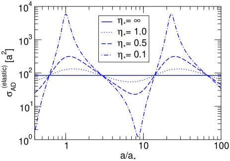
Figure 5: The elastic cross section for atom-dimer scattering at threshold in units of $a^{2}$ as a function of $a/a_{*}$ for several values of $\eta_{*}$.

If there are no deep dimers, atom-dimer scattering is completely elastic below the dimer-breakup threshold $ka=2/\sqrt{3}$. The existence of deep dimers opens up inelastic channels in which an atom and a shallow dimer with low energy collide to form an atom and a deep dimer. The large binding energy of the deep dimer is released through the large kinetic energies of the recoiling atom and dimer. This process is called dimer relaxation. The optical theorem implies that the total cross section for inelastic atom-dimer scattering near the atom-dimer threshold $E=-E_{D}$ is proportional to the imaginary part of the atom-dimer scattering length in Eq. (72):

$$\sigma_{AD}^{\rm(inelastic)}(E\to-E_{D}) \longrightarrow \frac{4\pi}{k}\;(-{\rm Im}\,a_{AD})\,.$$ (74)

Thus the cross section for dimer relaxation diverges like $1/k$ as $E$ approaches the atom-dimer threshold.

The event rate $\beta$ for dimer relaxation is defined so that the number of dimer relaxation events per time and per volume in a gas of atoms with number density $n_{A}$ and dimers with number density $n_{D}$ is $\beta n_{A}n_{D}$. If the atom and the deep dimer produced by the relaxation process have large enough kinetic energies to escape from the system, the rate of decrease in the number densities is

$${d\ \over dt}n_{A} = {d\ \over dt}n_{D}=-\beta n_{A}n_{D}\,.$$ (75)

The event rate $\beta$ can be expressed in terms of a statistical average of the inelastic atom-dimer cross section:

$$\beta={3\hbar\over 2m}\left\langle k\ \sigma_{AD}^{\rm(inelastic)}(E)\right\rangle\,.$$ (76)

In the low-temperature limit, $\beta$ reduces to $6\pi\hbar(-{\rm Im}\,a_{AD})/m$, which can be written as [38]

$$\beta = {20.3\sinh(2\eta_{*})\over\sin^{2}[s_{0}\ln(a/a_{*})]+\sinh^{2}\eta_{*}}\;{\hbar a\over m}\,.$$ (77)

If $\eta_{*}$ is small, the maximum value of $\beta$ occurs when $a\approx[1+\sinh^{2}\eta_{*}/(2s_{0}^{2})]a_{*}$.

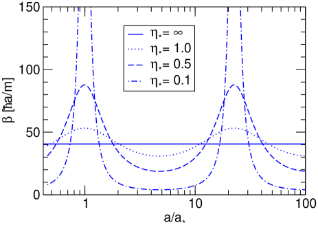
Figure 6: The dimer relaxation rate constant in units of $\hbar a/m$ as a function of $a/a_{*}$ for several values of $\eta_{*}$.

The coefficient of $\hbar a/m$ is shown in Fig. 6 as a function of $a/a_{*}$ for several values of $\eta_{*}$. It displays resonant behavior with maxima when the scattering length has one of the values $(e^{\pi/s_{0}})^{n}a_{*}$ for which the peak of an Efimov resonance is at the atom-dimer threshold. In the limit $\eta_{*}\to 0$, the maximum value $40.6\coth\eta_{*}$ of the coefficient of $\hbar a/m$ diverges. In the limit $\eta_{*}\to\infty$, the log-periodic dependence of the coefficient on $a\kappa_{*}$ disappears and it reduces to the constant 40.6.

5.4 Three-body recombination

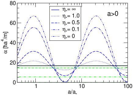
Figure 7: The 3-body recombination rate constants $\alpha_{\rm shallow}$ (with large-amplitude oscillations) and $\alpha_{\rm deep}$ (with small-amplitude oscillations) in units of $\hbar a^{4}/m$ as functions of $a/a_{*}$ for $a>0$ and several values of $\eta_{*}$.

If there are no deep dimers, the rate constant $\alpha_{\rm shallow}$ for 3-body recombination into the shallow dimer has the remarkable form given in Eq. (63), which has zeroes at values $a$ that differ by multiples of $e^{\pi/s_{0}}\approx 22.7$. If there are deep dimers, the analytic expression for the rate constant $\alpha_{\rm shallow}$ is

$$\alpha_{\rm shallow}={128\pi^{2}(4\pi-3\sqrt{3})(\sin^{2}[s_{0}\ln(a/a_{*0})]+\sinh^{2}\eta_{*})\over\sinh^{2}(\pi s_{0}+\eta_{*})+\cos^{2}[s_{0}\ln(a/a_{*0})]}\,{\hbar a^{4}\over m}\,,$$ (78)

where $a_{*0}\approx 4.5\,a_{*}$ is given in Eq. (64). We can use the approximation $\sinh(\pi s_{0}+\eta_{*})\approx e^{\eta_{*}}\sinh(\pi s_{0})$ to simplify the expression in Eq. (78):

$$\alpha_{\rm shallow} \approx 67.12\,e^{-2\eta_{*}}\left(\sin^{2}[s_{0}\ln(a/a_{*0})]+\sinh^{2}\eta_{*}\right)\hbar a^{4}/m.$$ (79)

The coefficient of $\hbar a^{4}/m$ is shown as a function of $a/a_{*}$ in Fig. 7 for several values of $\eta_{*}$. As $a$ varies, the coefficient of $\hbar a^{4}/m$ oscillates between about $67.12\,e^{-2\eta_{*}}\sinh^{2}\eta_{*}$ and about $67.12\,e^{-2\eta_{*}}\cosh^{2}\eta_{*}$. Thus one effect of the deep dimers is to eliminate the zeros in $\alpha_{\rm shallow}$ at $a=(e^{\pi/s_{0}})^{n}a_{*0}$. The depth of the minimum is quadratic in $\eta_{*}$ as $\eta_{*}\to 0$, so the coefficient of $\hbar a^{4}/m$ at $a=(e^{\pi/s_{0}})^{n}a_{*0}$ can be very small if the Efimov width parameter $\eta_{*}$ is small.

The existence of deep dimers opens up additional channels for 3-body recombination. If there are no deep dimers, 3-body recombination can only produce the shallow dimer if $a>0$ and it cannot proceed at all if $a<0$. If there are deep dimers, they can be produced by 3-body recombination for either sign of $a$. We denote by $\alpha_{\rm deep}$ the inclusive contribution to the event rate constant defined in Eq. (62) from 3-body recombination into all the deep dimers.

If $a>0$, the analytic expression for $\alpha_{\rm deep}$ is

$$\alpha_{\rm deep}={64\pi^{2}(4\pi-3\sqrt{3})\coth(\pi s_{0})\sinh(2\eta_{*})\over\sinh^{2}(\pi s_{0}+\eta_{*})+\cos^{2}[s_{0}\ln(a/a_{*0})]}\,{\hbar a^{4}\over m}\,,$$ (80)

where $a_{*0}\approx 4.5\,a_{*}$ is given in Eq. (64). The coefficient of $\hbar a^{4}/m$ has very weak log-periodic dependence on $a\kappa_{*}$. We can use the appproximation $\sinh(\pi s_{0}+\eta_{*})\approx e^{\eta_{*}}\sinh(\pi s_{0})$ to simplify the expression in Eq. (80):

$$\alpha_{\rm deep}\approx 16.84\left(1-e^{-4\eta_{*}}\right)\hbar a^{4}/m\,,\qquad(a>0)\,.$$ (81)

The numerical result for the coefficient in Eq. (81) was first derived in Ref. [38]. The coefficient of $\hbar a^{4}/m$, which is independent of $a/a_{*}$, is shown in Fig. 7 for several values of $\eta_{*}$. In the limit $\eta_{*}\to 0$, $\alpha_{\rm deep}$ approaches zero linearly in $\eta_{*}$. In the limit $\eta_{*}\to\infty$, the rates $\alpha_{\rm deep}$ in Eq. (80) and $\alpha_{\rm shallow}$ in Eq. (78) are almost equal, differing only by the factor $\coth(\pi s_{0})\approx 1.004$.

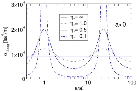
Figure 8: The 3-body recombination rate constant $\alpha_{\rm deep}$ in units of $\hbar a^{4}/m$ as a function of $a/a_{*}^{\prime}$ for $a<0$ and several values of $\eta_{*}$.

If $a<0$, the 3-body recombination rate constant is

$$\alpha_{\rm deep} = {4590\sinh(2\eta_{*})\over\sin^{2}[s_{0}\ln(a/a_{*}^{\prime})]+\sinh^{2}\eta_{*}}\;{\hbar a^{4}\over m}\,,\qquad(a<0)\,,$$ (82)

where $a_{*}^{\prime}\approx-1.6\,\kappa_{*}^{-1}$ is given in Eq. (56). The explicit formula for $\alpha_{\rm deep}$ in Eq. (82) was first derived in Ref. [38]. The coefficient 4590 is only known numerically. The coefficient of $\hbar a^{4}/m$ is shown as a function of $a/a_{*}^{\prime}$ in Fig. 8 for several values of $\eta_{*}$. It displays resonant behavior with maxima when the scattering length has one of the values $(e^{\pi/s_{0}})^{n}a_{*}^{\prime}$ for which there is an Efimov trimer near the 3-atom threshold. In the limit $\eta_{*}\to 0$, the maximum value $9180\coth\eta_{*}$ of the coefficient of $\hbar a^{4}/m$ in Eq. (82) diverges. In the limit $\eta_{*}\to\infty$, the log-periodic dependence of the coefficient on $a\kappa_{*}$ disappears and it approaches the constant 9180.

6 Applications to Atoms

In this section, we describe applications of universality to ⁴He atoms and to alkali atoms near a Feshbach resonance.

6.1 Helium atoms

Helium atoms provide a beautiful illustration of universality in the 3-body system [36]. The interatomic potential between two ⁴He atoms does not support any deep dimers, so universality is realized in its simplest form with a single 3-body parameter $\kappa_{*}$. The binding energies of the ⁴He trimers have been calculated accurately for a number of different model potentials for the interaction between two ⁴He atoms. For the purposes of illustration, we will use the TTY potential [9]. The scattering length for the TTY potential is $a=188.99\,a_{0}$. This is much larger than its effective range $r_{s}=13.85\,a_{0}$, which is comparable to the van der Waals length scale $\ell_{\rm vdw}=10.2\,a_{0}$. The TTY potential supports a single 2-body bound state, the ⁴He dimer whose binding energy is $E_{2}=1.30962$ mK. This binding energy is small compared to the natural low-energy scale for ⁴He atoms: $E_{\rm vdW}\approx 420$ mK. The TTY potential supports exactly two 3-body bound states: the ground-state trimer, which we label $n=0$, and the excited trimer, which we label $n=1$. There have been several accurate calculations of the binding energies $E_{3}^{(0)}$ and $E_{3}^{(1)}$ for the TTY potential [41, 42, 43]. The results agree to within 0.5% for both $E_{3}^{(0)}$ and $E_{3}^{(1)}$. The results of Ref. [42] are $E_{3}^{(0)}=126.4$ mK and $E_{3}^{(1)}=2.28$ mK.

The ⁴He dimer was first observed in 1992 by the Minnesota group [44]. They used the expansion of ⁴He gas at room temperature from a pulsed valve into a vacuum chamber to create a beam of ⁴He atoms and clusters with a translational temperature near 1 mK. The dimers were detected by using electron impact ionization to produce helium dimer ions that were observed by mass spectrometry. In another experiment in 1995, they determined the size of the ⁴He dimer by measuring the relative transmission rates of He atoms and dimers through a set of nanoscale sieves [45]. Their result for the mean separation of the atoms in the dimer was $\langle r\rangle=(62\pm 10)$ Å.

The ⁴He dimer was also detected nondestructively by the Göttingen group [46]. They made a beam of ⁴He atoms and clusters with temperature ranging from 6 K to 60 K by allowing cryogenic ⁴He gas to escape from an orifice. The beam was passed through a nanoscale transmission grating, and the dimers were detected by observing a diffraction peak at the expected angle. In 1995, this experiment was used to make the first observation of the ground state ⁴He trimer [4]. The excited ⁴He trimer has not yet been observed. In a subsequent experiment, the ⁴He tetramer was observed and the formation rates of dimers, trimers, and tretramers was measured as functions of the temperature and pressure of the gas from which the beam escaped [47]. In 2000, the Göttingen group determined the size of the dimer from the relative strengths of the higher order diffraction peaks from the nanoscale transmission grating [48]. Their result for the mean separation of the atoms is $\langle r\rangle=(52\pm 4)$ Å. This result is in good agreement with the theoretical prediction from the TTY potential: $\langle r\rangle=a/2=50$ Å. From this measurement, the binding energy of the ⁴He dimer was inferred to be $E_{2}=(1.1^{+0.3}_{-0.2})$ mK. The scattering length for ⁴He atoms was inferred to be $a=(104^{+8}_{-18})$ Å.

Lim, Duffy, and Damert proposed in 1977 that the excited state of the ⁴He trimer is an Efimov state [49]. This interpretation is almost universally accepted. Some researchers have proposed that the ground state trimer is also an Efimov state [18, 50, 51]. This raises an obvious question: what is the definition of an Efimov state? The most commonly used definition is based on rescaling the depth of the 2-body potential: $V({\bf r})\longrightarrow\lambda V({\bf r})$. According to the traditional definition, a trimer is an Efimov state if its binding energy as a function of the scaling parameter $\lambda$ has the qualitative behavior illustrated in Fig. 4. As $\lambda$ is decreased below 1, the trimer eventually disappears through the 3-atom threshold. As $\lambda$ is increased above 1, the trimer eventually disappears through the atom-dimer threshold. Calculations of the trimer binding energies [52] using a modern helium potential show that the excited trimer satisfies this definition of an Efimov state but the ground state trimer does not. The excited trimer disappears through the 3-atom threshold when $\lambda$ is decreased to about $0.97$, and it disappears through the atom-dimer threshold when $\lambda$ is increased to about 1.1. The ground state trimer disappears through the 3-atom threshold when $\lambda$ is about $0.9$. However, as $\lambda$ is increased above 1, its binding energy relative to the atom-dimer threshold continues to increase. Thus the ground state ⁴He trimer does not qualify as an Efimov state by the traditional definition.

The traditional definition of an Efimov state described above is not natural from the point of view of universality. The essence of universality concerns the behavior of a system when the scattering length becomes increasingly large. The focus of the traditional definition is on the endpoints of the binding energy curve in Fig. 4, which concerns the behavior of the system as the scattering length decreases in magnitude. The problem is that the rescaling of the potential can move the system outside the universality region defined by $|a|\gg r_{s}$ before the trimer reaches the atom-dimer threshold. We therefore propose a definition of an Efimov state that is more natural from the universality perspective. A trimer is defined to be an Efimov state if a deformation that tunes the scattering length to $\pm\infty$ moves its binding energy along the universal curve illustrated in Fig. 4. The focus of this definition is on the resonant limit where the binding energy crosses the $1/a=0$ axis. In particular, the binding energy at this point should be larger than that of the next shallowest trimer by about a factor of 515. In the case of ⁴He atoms, the resonant limit can be reached by rescaling the 2-body potential by a factor $\lambda\approx 0.97$ [52]. At this point, the binding energy of the ground state trimer is larger than that of the excited trimer by about a factor of 570. The closeness of this ratio to the asymptotic value 515 supports the hypothesis that the ground state ⁴He trimer is an Efimov state.

In order to apply the universal predictions for low-energy 3-body observables to the case of ⁴He atoms, we need a 2-body input and a 3-body input to determine the parameters $a$ and $\kappa_{*}$. The scattering length $a=188.99\,a_{0}$ for the TTY potential can be taken as the 2-body input. An alternative 2-body input is the dimer binding energy: $E_{2}=1.31$ mK. A scattering length $a_{D}$ can be determined by identifying $E_{2}$ with the universal binding energy of the shallow dimer: $E_{2}=\hbar^{2}/(ma_{D}^{2})$. The result for the TTY potential is $a_{D}=181.79\,a_{0}$. The 3.8% difference between $a$ and $a_{D}$ is a measure of how close the system is to the scaling limit. To minimize errors associated with the deviations of the system from the scaling limit, it is best to take the shallowest 3-body binding energy available as the input for determining $\kappa_{*}$. In the case of ⁴He atoms, this is the binding energy $E_{3}^{(1)}$ of the excited trimer. Experience has shown that the universal predictions are considerably more accurate if $E_{2}$ and $E_{3}^{(1)}$ are used as the inputs instead of $a$ and $E_{3}^{(1)}$ [36].

We proceed to consider the universal predictions for the trimer binding energies. Having identified $E_{3}^{(1)}$ with the universal trimer binding energy $E_{T}^{(1)}$, we can use Efimov’s binding energy equation (44) with $n_{*}=1$ to calculate $\kappa_{*}$ up to multiplicative factors of $e^{\pi/s_{0}}\approx 22.7$ [36]. The result is $\kappa_{*}=0.00215\,a_{0}^{-1}$ or $\kappa_{*}=0.00232\,a_{0}^{-1}$, depending on whether $E_{2}$ or $a$ is used as the 2-body input. The intuitive interpretation of $\kappa_{*}$ is that if a parameter in the short-distance potential is adjusted to tune $a$ to $+\infty$, the binding energy $E_{3}^{(1)}$ should approach a limiting value of approximately $\hbar^{2}\kappa_{*}^{2}/m$, which is 0.201 mK or 0.233 mK depending on whether the 2-body input is $E_{2}$ or $a$.

	$a$	$a_{D}$	$E_{3}^{(1)}$	$E_{3}^{(0)}$	$E_{3}^{(-1)}$
TTY potential	100.0	96.2	2.28	126.4	–
universality		input	input	129.1	$5.38\times 10^{4}$
universality	input		input	146.4	$6.23\times 10^{4}$

Table 1: Binding energies $E_{3}^{(n)}$ of the ⁴He trimers for the TTY potential (row 1) compared to the universality predictions using as the inputs either $E_{2}$ and $E_{3}^{(1)}$ (row 2) or $a$ and $E_{3}^{(1)}$ (row 3). Lengths are given in Å and energies are given in mK. The trimer binding energies for the TTY potential are from Ref. [42]. (Note that $\hbar^{2}/m=12.1194$ KŲ for ⁴He atoms.)

Once $\kappa_{*}$ has been calculated, we can solve Eq. (44) for the binding energies of the deeper Efimov states. The prediction for the next two binding energies are shown in Table 1. The prediction for $E_{3}^{(0)}$ differs from the binding energy of the ground-state trimer by 2.6% or 16.4%, depending on whether $E_{2}$ or $a$ is taken as the 2-body input. The expected order of magnitude of the error is the larger of $\ell_{\rm vdW}/a=5.4$% and $(E_{3}^{(0)}/E_{\rm vdW})^{1/2}\approx 50$%. The errors are much smaller than $(E_{3}^{(0)}/E_{\rm vdW})^{1/2}$, suggesting that the scaling limit is more robust than one might naively expect. Efimov’s equation (44) also predicts infinitely many deeper 3-body bound states. The predictions for the binding energy $E_{3}^{(-1)}$ of the next deepest state are given in Table 1. The predictions are more than two orders of magnitude larger than the van der Waals $E_{\rm vdW}\approx 420$ mK. We conclude that this state and all the deeper bound states are artifacts of the scaling limit.

Using the above values of $\kappa_{*}$ for the TTY potential, we can immediately predict the atom-dimer scattering length $a_{AD}$. If $a$ is used as the 2-body input, we find $a_{AD}\approx 0.94\,a$, corresponding to $a_{AD}\approx 178\,a_{0}$. If $E_{2}$ is used as the 2-body input, we find $a_{AD}\approx 1.19\,a_{D}$, corresponding to $a_{AD}\approx 216\,a_{0}$. These values are in reasonable agreement with the calculation of Ref. [43], which gave $a_{AD}=248(10)\,a_{0}$. Since $r_{s}/a=7.3$% for the TTY potential, much of the remaining discrepancy can perhaps be attributed to effective-range corrections.

Universality can also be used to predict the 3-body recombination rate constant for ⁴He atoms interacting through the TTY potential. The prediction for $\alpha_{\rm shallow}$ is $2.9\,\hbar a_{D}^{4}/m$ or $6.9\,\hbar a^{4}/m$, depending on whether $E_{2}$ or $a$ is used as the 2-body input. In either case, the coefficient of $\hbar a^{4}/m$ is much smaller than the maximum possible value 67.1. Thus ⁴He atoms are fortuitously close to a combination of $a$ and $\kappa_{*}$ for which $\alpha_{\rm shallow}$ is zero. The 3-body recombination rate constant has not yet been calculated for the TTY potential. It has been calculated for the HFD-B3-FCI1 potential [53]. The result is $\alpha_{\rm shallow}=12\times 10^{-29}$ cm⁶/s [37], which compares well with the universal prediction $9\times 10^{-29}$ cm⁶/s obtained using $E_{2}$ and $E_{3}^{(1)}$ as the inputs [6].

6.2 Alkali atoms near a Feshbach resonance

Alkali atoms near a Feshbach resonance provide a unique window on Efimov physics, because the scattering length can be tuned experimentally. Inelastic loss rates have proved to be an especially powerful probe of 3-body processes in these systems. In this subsection, we discuss some key experiments on 3-body losses for ²³Na, ⁸⁵Rb, ⁸⁷Rb, and ¹³³Cs atoms near Feshbach resonances and compare them with the predictions from universality.

The first observation of the enhancement of inelastic losses near a Feshbach resonance was by the MIT group [14]. They created Bose-Einstein condensate of ²³Na atoms in the $|1,+1\rangle$ hyperfine state and used a magnetic field to adjust the scattering length. They observed enhanced losses near the Feshbach resonances at 907 G and 853 G. Since the $|1,+1\rangle$ state is the lowest hyperfine state, the inelastic losses come primarily from 3-body recombination. The 3-body losses near the Feshbach resonance at 907 G were studied systematically by the MIT group [15]. They also studied 3-body losses in a Bose-Einstein condensate of ²³Na atoms in the $|1,-1\rangle$ hyperfine state near a Feshbach resonance at 1195 G. The off-resonant scattering length in this region of high magnetic field is approximately 52 $a_{0}$, which is significantly smaller than the van der Waals scale $\ell_{\rm vdW}\approx 90\,a_{0}$. Near the Feshbach resonances at 907 G, the authors of Ref. [15] were able to increase the scattering length by about a factor of 5 over the off-resonant value. However this it still not very large compared to the $\ell_{\rm vdW}$, so the universal theory does not apply. A quantitative description of the data on 3-body recombination near the 907 G resonance has been given using a scattering model for a Feshbach resonance with zero off-resonant scattering length [54].

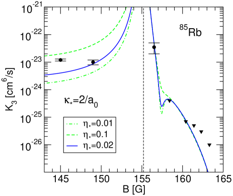
Figure 9: The 3-body loss coefficient $K_{3}$ in ⁸⁵Rb as a function of the magnetic field near the Feshbach resonance at $B=155$ G. The dots are the measured values of $K_{3}$ from Ref. [55], while the triangles indicate upper bounds on $K_{3}$. The curves are for $\kappa_{*}a_{0}=2$ and several values of $\eta_{*}$.

The inelastic collision rate for ultracold ⁸⁵Rb atoms in the $|2,-2\rangle$ hyperfine state near the Feshbach resonance at 155 G has been studied by the JILA group [55]. By exploiting the different dependences on the number density, they were able to separate the contributions from 2-body and 3-body processes. They measured the 2-body and 3-body loss coefficients as a function of the magnetic field $B$ from 110 G to 150 G. At some values of $B$, they were only able to obtain an upper bound on the 3-body loss coefficient $K_{3}=3\alpha$. Their results for $K_{3}$ near the Feshbach resonance at 155 G are shown in Fig. 9. The universal results for the 3-body recombination rate at threshold are given by Eq. (82) for $a<0$ and they can be approximated by the sum of Eqs. (79) and (81) for $a>0$. A precise determination of the Efimov parameters $\kappa_{*}$ and $\eta_{*}$ is not possible with the data in Fig. 9. However as shown in Fig. 9, the data can be described reasonably well by the universal formulas with the values $\kappa_{*}a_{0}=2$ and $\eta_{*}=0.02$. The curves for different values of $\eta_{*}$ illustrate how the minima in the recombination rate for $a>0$ are filled by recombination into deep bound states.

The 3-body losses in ultracold ⁸⁷Rb were studied by the Garching group [56]. Roughly 90% of the atoms were in the $|1,+1\rangle$ hyperfine state. Most of the remaining atoms were in the $|1,0\rangle$ state, but there were also some atoms in the $|1,-1\rangle$ state. By monitoring the atom loss, the authors observed more than 40 Feshbach resonances for various combinations of hyperfine states of ⁸⁷Rb at magnetic fields ranging from 300 G to 1300 G. Measurements of the resonances were used to deduce an improved atomic potential for ⁸⁷Rb. Away from the Feshbach resonances, the scattering lengths for ⁸⁷Rb have natural values comparable to the van der Waals scale $\ell_{\rm vdW}\approx 165\,a_{0}$. The 3-body loss rate $K_{3}=3\alpha$ in the vicinity of the resonance at 1007 G was measured as a function of the magnetic field. Away from the resonance, $K_{3}$ was measured to be $3.2(1.6)\times 10^{-29}$ cm⁶/s. Near the resonance, the rate constant was observed to increase by as much as a factor of 300.

The 3-body recombination rate in a Bose-Einstein condensate of ⁸⁷Rb atoms in the $|1,+1\rangle$ hyperfine state has been measured just below the Feshbach resonance at 1007 G by the Garching group and by the Oxford group [57]. The values of the magnetic fields ranged from about 1 G below the resonance, where the scattering length has a natural value comparable to the van der Waals scale $\ell_{\rm vdW}\approx 165\,a_{0}$, to about 0.03 G below the resonance, where the scattering length is about a factor 5 larger than $\ell_{\rm vdW}$. Only the last few data points are in the universal region. The measured rate constant $K_{3}=3\alpha$ appears to scale as a smaller power of $a$ than the scaling prediction $a^{4}$. The measurements of $K_{3}$ agree reasonably well with the results of exact solutions to the 3-body Schrödinger equation for a coupled-channel model [57]. These calculations predict a local minimum of $K_{3}$ that can be attributed to Efimov physics at a magnetic field about 0.015 G below the resonance, just outside the range of the experiments. The atom-dimer relaxation rate for the coupled-channel model was also calculated in Ref. [57]. The model predicts a resonance in the relaxation rate less than 0.1 G below the resonance.

The 3-body recombination rate for an ultracold gas of ¹³³Cs atoms in the $|3,+3\rangle$ hyperfine state was measured as a function of the magnetic field by the Innsbruck group [58]. The 3-body recombination loss rate $K_{3}=3\alpha$ is very small near 17 G, where the scattering length goes through a zero that comes from the interplay between a broad Feshbach resonance and the large off-resonant scattering length for ¹³³Cs. For magnetic fields between 50 G and 150 G, the measurements confirmed the $a^{4}$ power-law dependence of $K_{3}$ predicted by scaling. In this region of the magnetic field, the scattering length increased from about 1000 $a_{0}$ to about 1600 $a_{0}$. Since the scattering length increased only by a factor of 1.6, it was not possible to observe any logarithmic variations of the coefficient of $a^{4}$.

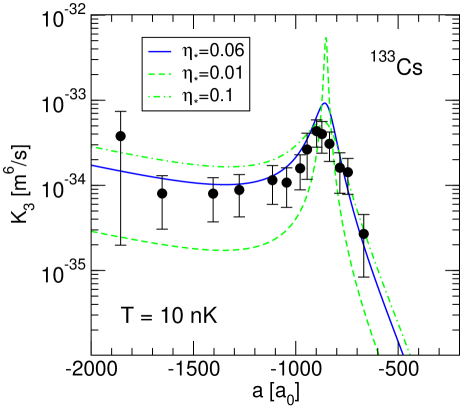
Figure 10: The 3-body loss coefficient $K_{3}$ in ¹³³Cs for negative values of the scattering length near the Efimov resonance at $a\approx-850\,a_{0}$. The data points are for $T=10$ nK and are taken from Ref. [5]. The curves are for $\kappa_{*}=0.945/a_{0}$ and three different values of $\eta_{*}$.

The Innsbruck group extended their measurement of the 3-body recombination loss rate $K_{3}=3\alpha$ for ¹³³Cs atoms in the $|3,+3\rangle$ hyperfine state to values of the magnetic field below 17 G where the scattering length is negative [5]. The negative scattering length could be made as large as $-2500\,a_{0}$. They observed a resonant enhancement of $K_{3}$ for $a$ near $-800\,a_{0}$. The enhancement can be explained by the presence of an Efimov state near the 3-atom threshold. At the lowest temperature they were able to reach, which was 10 nK, the shape of the resonance could be fit reasonably well using the universal result in Eq. (82), which has a peak near $a_{*}$. The best fit values of the Efimov parameters are $a_{*}^{\prime}=-850(20)\,a_{0}$ and $\eta_{*}=0.06(1)$. In Fig. 10, we compare the data of Ref. [5] with the universal result. The parameters $a_{*}^{\prime}=-850\,a_{0}$ (which corresponds to $\kappa_{*}=0.945\,a_{0}^{-1}$) and $\eta_{*}=0.06$ give a good fit to the data. Both Efimov parameters are well determined by the data: $\kappa_{*}$ by the position of the Efimov resonance and $\eta_{*}$ by the height and width of the peak. Since the van der Waals length scale for ¹³³Cs is $\ell_{\rm vdW}\approx 200\,a_{0}$, the resonance is reasonably deep into the universal region. Thus these results from Innsbruck group seem to be the first experimental evidence for the existence of Efimov states [5].

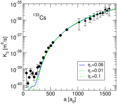
Figure 11: The 3-body loss coefficient $K_{3}$ in ¹³³Cs for positive values of the scattering length. The data points are for $T=200$ nK (dots) and for temperatures between 250 nK and 400 nK (triangles) and they are taken from Ref. [5]. The curves are for $\kappa_{*}=0.707/a_{0}$ and three different values of $\eta_{*}$.

The Innsbruck group also carried out a more careful analyisis of 3-body recombination at magnetic fields above 170 G, where $a$ is positive [5]. They measured the loss rate $K_{3}$ with higher accuracy and at more values of the magnetic field. They observed a local minimum in the atom loss rate for $a$ near $210\,a_{0}$. The dependence of the loss rate constant $K_{3}$ on the scattering length can be fit reasonably well with the universal formula given by the sum of Eqs. (79) and (81). The value of $\eta_{*}$ is not well determined by the data and the fit yields only the upper bound $\eta_{*}<0.2$. The best fit for the value of $a$ at which the coefficient of $a^{4}$ is maximal is $a_{+}=1060(70)\,a_{0}$. This corresponds to $a_{*}\approx 1170\,a_{0}$. The positive scattering length data from Ref. [5] are shown in Fig. 11. The Efimov parameter $\kappa_{*}=0.707\,a_{0}^{-1}$ corresponding to $a_{*}=1170\,a_{0}$ gives a good fit to the data above $a\approx 400\,a_{0}$. If the scattering length could be increased past $\infty$ to a region where $a$ is large and negative, universality predicts that there should be an Efimov state at the 3-atom threshold when $a$ is approximately $-1100\,a_{0}$. This is not far (at least on a log scale) from the position $-850\,a_{0}$ where the resonance was observed. However the region of large negative $a$ in which the resonance is observed is separated from the region of large positive $a$ by a region where $a$ passes through zero and universal theory does not apply. As a consequence, the Efimov parameters for the two regions need not be equal. One note of caution in applying the universal expression for the 3-body recombination rate at threshold is that the positive scattering length data in Fig. 11 was obtained at temperatures that ranged from 200 nK to 400 nK, which is much larger than the temperature 10 nK for the negative scattering length data in Fig. 10. The temperature for the positive scattering length data may not be low enough to use the universal expression for the 3-body recombination rate at threshold.

The Innsbruck group has also observed inelastic losses of shallow dimers composed of ¹³³Cs atoms in the $|3,+3\rangle$ hyperfine state [59]. The fraction of dimers that are lost remains roughly constant for magnetic fields in the range from between 14 G and 19.8 G. However, the fraction increases rapidly toward 1 as the magnetic field increases further toward a Feshbach resonance at 19.84 G. In this experiment, resonant enhancements of the inelastic loss rate were also observed at lower values of the magnetic field. They can be attributed to effects of a ¹³³Cs tetramer near the threshold for two ¹³³Cs dimers. In this region of the magnetic field, the dimers are deeply bound, so these results have nothing to do with universality.

Very recently, the Innsbruck group has created mixtures of ¹³³Cs atoms in the $|3,+3\rangle$ hyperfine state and shallow dimers composed of those atoms [60]. They have observed a resonance enhancement in the inelastic atom-dimer collision rate near $a\approx 400\ a_{0}$ [60]. The enhancement can be explained by the presence of an Efimov state near the atom-dimer threshold. They have measured the rate constant $\beta$ defined by Eq. (75) as a function of the magnetic field at a temperature near 250 nK. The universal predictions for $\beta$ as a function of $T$ have been calculated for temperatures small compared to the binding energy of the shallow dimer. It might be possible to use these measurements to determine the Efimov parameters $a_{*}$ and $\eta_{*}$ accurately for this region of large positive scattering length [61].

7 Efimov Physics in Other Three-body Systems

Very few universal results have been calculated for 3-body systems other than identical bosons. They are summarized in Ref. [6]. In this section, we consider only the basic question of whether the Efimov effect occurs in the 3-body system. This question can be answered by determining the channel eigenvalue $\lambda_{0}(R)$ for the lowest hyperspherical potential in the scaling limit. The Efimov effect occurs if $\lambda_{0}(R)$ is negative at $R=0$. If $\lambda_{0}(0)=-s_{0}^{2}$, the discrete scaling factor for Efimov physics is $e^{\pi/s_{0}}$.

7.1 Unequal scattering lengths

There are 3-body systems in atomic physics in which the three atoms all have the same mass, but the three pairs of atoms need not all have the same scattering lengths. For example, different hyperfine spin states of the same atom have the same mass, but the scattering lengths $a_{ij}$ can be different for each pair $ij$ of hyperfine states. As another example, different isotopes of a heavy atom have nearly the same masses. It is therefore worthwhile to consider the universal behavior of systems with equal masses and with scattering lengths that are large but not necessarily equal.

The Efimov effect in general 3-body systems was first discussed by Amado and Noble [62] and by Efimov [63, 64]. A summary of their results is as follows. If only one of the three scattering lengths is large, the Efimov effect does not occur. If two of the scattering lengths are large, the Efimov effect occurs with a discrete scaling factor of 1986.1 unless two of the three particles are identical fermions, in which case the Efimov effect does not occur. If all three scattering lengths are large, the Efimov effect occurs with a discrete scaling factor of 22.7. For a derivation of these results, see Ref. [6].

If the atoms are distinguishable but related by an internal symmetry, the condition for the Efimov effect is modified. An example is the spin states belonging to a hyperfine multiplet at zero magnetic field, which are related by a spin symmetry. A general treatment of the effects of an internal symmetry was given by Bulgac and Efimov in Ref. [65].

7.2 Unequal masses

In the 2-body sector, the universal results for particles of unequal masses are only a little more complicated than those for the equal-mass case in Sections 3.1 and 3.2. Let the atoms 1 and 2 have a large scattering length $a_{12}$ and unequal masses $m_{1}$ and $m_{2}$. If $a_{12}$ is large and positive, the atoms 1 and 2 form a shallow dimer with binding energy

$$E_{D}={\hbar^{2}\over 2m_{12}a_{12}^{2}}\,,$$ (83)

where $m_{12}=m_{1}m_{2}/(m_{1}+m_{2})$ is the reduced mass.

In the general 3-body system, the three masses can be unequal and any combination of the three scattering lengths can be large. The Efimov effect in general 3-body systems was first discussed by Amado and Noble [62] and by Efimov [63, 64]. The special case in which two of the three particles have the same mass was also discussed by Ovchinnikov and Sigal [66]. The conditions for the existence of the Efimov effect and the value of the discrete scaling factor depend on the ratios of the masses. We first summarize the results for the extreme cases in which two masses are equal and the third mass is either much larger or much smaller. In the case of two heavy particles and one light particle, the Efimov effect occurs provided the heavy-light scattering length is large. The Efimov effect can be understood intuitively in this case by using the Born-Oppenheimer approximation [67]. In the case of one heavy particle and two light particles, the Efimov effect occurs only if all three pairs of particles have large scattering lengths.

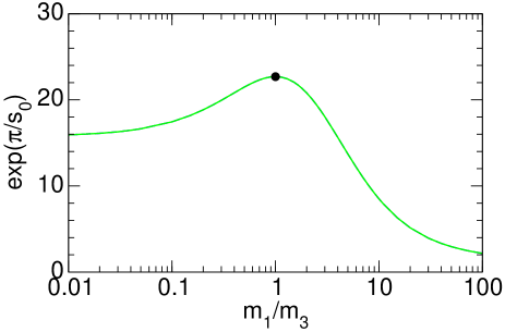
Figure 12: Discrete scaling factor $e^{\pi/s_{0}}$ for two particles of equal mass $m_{1}=m_{2}$ as a function of the mass ratio $m_{1}/m_{3}$ for the case in which all three pairs have large scattering lengths. The particles 1 and 2 can be either identical bosons or distinguishable. The dot indicates the case of three identical bosons.

We next consider a more general case in which all three pairs of atoms have a large scattering length. This excludes the possibility of any pair of particles being identical fermions. The condition for the Efimov effect does not depend on the values of the scattering lengths as long as their absolute values are large compared to the range. The Efimov effect occurs for any values of the masses. The discrete scaling factor is largest if all three masses are equal. It has the same value $e^{\pi/s_{0}}\approx 22.7$ as for three identical bosons. In the case of two equal-mass particles, the discrete scaling factor is the same whether the equal-mass particles are identical bosons or distinguishable. The discrete scaling factor for $m_{1}=m_{2}$ is shown as a function of the mass ratio $m_{1}/m_{3}=m_{2}/m_{3}$ in Fig. 12. In the limit $m_{1}=m_{2}\ll m_{3}$, the discrete scaling factor approaches $15.7$. In the limit $m_{1}=m_{2}\gg m_{3}$, it approaches 1.

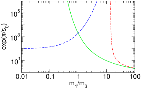
Figure 13: Discrete scaling factor $e^{\pi/s_{0}}$ for two particles of equal mass $m_{1}=m_{2}$ as a function of the mass ratio $m_{1}/m_{3}$ for the cases in which two pairs have large scattering lengths. If $a_{23}$ and $a_{31}$ are large, particles 1 and 2 can be either identical bosons or distinguishable particles (solid line) or else identical fermions (dash-dotted line). If $a_{12}$ and $a_{31}$ (or $a_{12}$ and $a_{23}$) are large, particles 1 and 2 must be distinguishable particles (dashed line).

We now consider the more general case in which only two pairs of atoms have large scattering lengths. For simplicity, we consider only the special cases in which particles 1 and 2 have the same masses $m_{1}=m_{2}$. There are three cases to consider. The discrete scaling factors are shown in Fig. 13 as a function of the mass ratio $m_{1}/m_{3}$ for all three cases. If the large scattering lengths are $a_{23}$ and $a_{31}$ and if particles 1 and 2 are either identical bosons or distinguishable, the discrete scaling factor $e^{\pi/s_{0}}$ decreases monotonically from $\infty$ to 1986. If the large scattering lengths are $a_{23}$ and $a_{31}$ and if particles 1 and 2 are identical fermions, the Efimov effect occurs only if $m_{1}/m_{3}$ exceeds the critical value 13.607. The discrete scaling factor decreases monotonically from $\infty$ to 1 as $m_{1}/m_{3}$ increases from the critical value to $\infty$. If the large scattering lengths are $a_{12}$ and $a_{31}$ (or $a_{12}$ and $a_{23}$), particles 1 and 2 must be distinguishable. The discrete scaling factor increases monotonically from 94.36 to 1986.1 to $\infty$ as $m_{1}/m_{3}$ increases from 0 to 1 to $\infty$.

8 Extensions and Outlook

In this section, we discuss extensions of universality beyond the 3-body problem in the scaling limit: effective-range corrections, microscopic models with a large scattering length, and the 4-body problem. We end this review with an outlook on the study of Efimov physics.

8.1 Effective range corrections

The scaling limit of a system with a large scattering length is the limit in which the range of the interaction is taken to zero. There are corrections to the scaling limit from the fact that the range for any physical system is nonzero. These corrections can be calculated as an expansion in powers of $\ell/a$, where $\ell$ is the natural low-energy length scale. The most important corrections come from the effective range $r_{s}$, which is defined by the expansion of the S-wave phase shift in Eq. (5). Examples of effective range corrections for 2-body observables are given in Eqs. (33) and (34).

The most important correction to the scaling limit in the 3-body system also comes from the effective range $r_{s}$. At first order in the expansion in $\ell/|a|$, the effective range is the only new parameter that enters. Efimov has shown that the effective range leads to a correction term $r_{s}/R^{3}$ in the scale-invariant hyperspherical potential in Eq. (21) [68]. He gave expressions for the first-order effective range corrections to the binding energy of the Efimov trimer and to the atom-dimer scattering length [69]. Moreover, he applied his results to the 3-nucleon system, calculating the range corrections to the correlation between the triton binding energy and the spin-doublet neutron-deuteron scattering length [70] and to the spin-quartet neutron-deuteron scattering length [69].

Here, we will give only a brief summary of the systematics of higher-order range corrections in channels where the Efimov effect occurs. For a more complete discussion, we refer the reader to our longer review [6]. Since the correction to the universal long-range potential is singular, the range corrections require renormalization. Effective field theory provides a powerful framework to deal with these naively divergent corrections. The first-order effective range correction to the spin-doublet neutron-deuteron scattering phase shifts was first calculated using this method in [71] and later confirmed using a different renormalization scheme [72]. The systematics of contributions beyond first order in $\ell/|a|$ was studied by various authors [73, 74, 75, 76, 77]. The first calculation of the triton channel of the 3-nucleon system at second order in $\ell/|a|$ was carried out in Ref. [73]. As suggested by naive dimensional analysis, a new 3-body parameter was included in this calculation at order $(\ell/|a|)^{2}$. Recently, Platter and Phillips revisited this problem using a subtractive renormalization scheme. They found that the scattering amplitudes could be renormalized at order $(\ell/|a|)^{2}$ without the need of a new subtraction constant [76, 77]. According to their analysis, a new 3-body parameter is not required until at least order $(\ell/|a|)^{3}$. They applied their method to the system of ⁴He atoms and found good convergence of the expansion in $\ell/|a|$ [76].

8.2 Microsopic models

Since the low-energy behavior of particles with large scattering lengths is insensitive to the details of their interactions at short distances, the potential provides an inefficient encoding of the relevant physics. The sensitivity to short distances enters primarily through the scattering length and other constants that describe low-energy scattering. This motivates a more phenomenological approach in which the interactions are described by a scattering model, which can be specified by a parameterization of low-energy scattering amplitudes. The parameters of the scattering model can be treated as phenomenological parameters that can be tuned to reproduce the observed low-energy observables of the 2-body system. Scattering models will exhibit universal low-energy behavior as the scattering length $a$ is tuned to $\pm\infty$. Low-energy 3-body observables reduce in this limit to functions of $a$ and the Efimov parameters $\kappa_{*}$ and $\eta_{*}$, all of which are functions of the parameters of the scattering model.

An example of a scattering model that may provide an accurate description of atoms near a Feshbach resonance is the resonance model [78]. This model provides a natural description of atoms that have a weak coupling to a closed channel in which there is a diatomic molecule extremely close to the atom-atom threshold. The resonance model has three parameters that can be defined by specifying the S-wave phase shift $\delta_{0}(k)$:

$$k\cot\delta_{0}(k)=-\left[\lambda+\frac{g^{2}}{k^{2}-\nu}\right]^{-1}\,.$$ (84)

The scattering length and the effective range are $a=\lambda-g^{2}/\nu$ and $r_{s}=-2(g-\nu\lambda/g)^{2}$, respectively. Thus the effective range is negative definite. The approximation in Eq. (8) for the scattering length as a function of the magnetic field $B$ for an atom near a Feshbach resonance can be reproduced by taking $\lambda$ and $g$ to be independent of $B$ and $\nu$ to be linear in $B-B_{\rm res}$. Thus $\lambda$ can be identified with the off-resonant scattering length, $\nu$ is proportional to the detuning energy of a molecule in a closed channel, and $g$ is the strength of the coupling to the closed channel. The resonance model will exhibit universal behavior as $\nu$ is tuned to zero. Three-body observables will approach universal functions of $a$, $\kappa_{*}$, and $\eta_{*}$. The Efimov parameter $\kappa_{*}$ must be a function of $\lambda$ and $g$, while $\eta_{*}$ must be a function of the dimensionless combination $\lambda g^{2}$.

Some 3-body observables have been calculated in the resonance model in the special case $\lambda=0$ [54]. The scattering length and the effective range are $a=-g^{2}/\nu$ and $r_{s}=-2/g^{2}$, respectively. It is convenient to define a parameter $R_{*}=1/g^{2}$, with dimension of length. The atom-dimer scattering length $a_{AD}$ and the 3-body recombination rate into the shallow dimer $\alpha$ have been calculated in this model as functions of $a$ and $R_{*}$ [54]. For $a\gg R_{*}$, they have the universal behavior given in Eqs. (61) and (63). The 3-body parameter $\kappa_{*}$ was determined in Ref. [54] to be

$$s_{0}\ln(\kappa_{*})=s_{0}\ln(2.5/R_{*})\mod\pi\,.$$ (85)

The cross-over to the universal behavior occurs when $a$ is comparable to $R_{*}$. The first divergence of the atom-dimer scattering length occurs at $a=0.45\,R_{*}$. This marks the emergence of the first Efimov state below the atom-dimer threshold. The second and higher divergences of $a_{AD}$ occur at values of $a$ that are well-approximated by the universal predictions: $a=(e^{\pi/s_{0}})^{n}\,0.64\,R_{*}$, $n=1,2,\dots$, where $e^{\pi/s_{0}}\approx 22.7$. The first zero of the recombination rate constant occurs at $a=3.3\,R_{*}$. The second and higher zeroes occur at values of $a$ that are well approximated by the universal predictions: $a=(e^{\pi/s_{0}})^{n}\,2.9\,R_{*}$, $n=1,2,\dots\;$.

8.3 Four-body problem

In the 3-body problem, exact numerical solutions are facilitated by the Faddeev equations. The generalization of the Faddeev equations to the $N$-body problem with $N\geq 4$ was given by Yakubovsky [79]. An equivalent set of equations was given independently by Grassberger and Sandhas [80]. Due to the complexity of these equations, exact numerical solutions for $N=4$ have only recently been obtained. In atomic physics, the only numerically exact $N$-atom calculations for $N\geq 4$ that we are aware of are for ground-state binding energies. There are no such calculations for weakly-bound $N$-atom molecules that might be governed by universality.

Testing universality in systems with four and more particles is a new frontier. Even theoretically, the universal properties in the 4-body sector are not fully understood. An important issue in the 4-body system with a large scattering length is how many parameters are required to describe the system in the scaling limit, that is, up to corrections that decrease like $\ell/|a|$ as $a\to\pm\infty$. In the case of identical bosons, low-energy 4-body observables necessarily depend on the 2-body parameter $a$ and the 3-body parameter $\kappa_{*}$. But are any additional 4-body parameters required? There are theoretical arguments in support of both answers to this question. There is a renormalization argument for zero-range 2-body potentials that indicates that an additional $N$-body parameter is required to calculate $N$-body binding energies for all $N\geq 3$ [81]. On the other hand, a power-counting argument within the effective field theory framework suggests that after adding the 3-body parameter $\kappa_{*}$, no additional parameters are necessary to calculate $N$-body observables for $N\geq 4$ [82].

Platter et al. have recently studied the universal properties of the system of four identical bosons with short-range interactions in an effective quantum mechanics approach [83]. They constructed the effective interaction potential at leading order in the large scattering length and computed the 4-body binding energies using the Yakubovsky equations. They found that cutoff independence of the 4-body binding energies does not require the introduction of a 4-body parameter at leading order in $\ell/|a|$. This suggests that 2-body and 3-body interactions are sufficient to renormalize the 4-body system. They applied their equations to ⁴He atoms and calculated the binding energies of the ground state and the excited state of the ⁴He tetramer. Using the binding energy $E_{2}$ of the ⁴He dimer as the 2-body input and the binding energy $E_{3}^{(1)}$ of the excited state of the ⁴He trimer as the 3-body input, they found good agreement with results of Blume and Greene [84] calculated using an approximate numerical method that combines Monte Carlo methods with the hyperspherical expansion.

Yamashita et al. [85] recently claimed that for a 4-body system close to a Feshbach resonance, a new 4-body parameter will enter already at leading order in $\ell/|a|$. They motivated their claim from a model-space reduction of a realistic 2-body interaction. In the framework of the renormalized zero-range model, they found a strong sensitivity of the 4-body ground state energy to a 4-body subtraction constant in their equations. The results of Ref. [83] for the special case of ⁴He atoms were also reproduced. A drawback of their analysis is the focus on the deepest 4-body state only. It remains to be seen whether their findings are universal or just artefacts of their regularization of the renormalized zero-range model.

8.4 Outlook

Vitaly Efimov’s discovery in 1970 of the Efimov effect in identical bosons was like finding a nugget of a precious metal. Other physicists quickly verified the amazing properties of this nugget and tried to find similar nuggets in other systems. Efimov went on to show that the nugget came from a rich vein of ore corresponding to universal properties of 3-body systems with a large scattering length. He pointed out that the Efimov effect was just a hint of a discrete scaling symmetry, and showed how the discrete scaling symmetry could be exploited to mine the ore. However not many physical systems in which Efimov physics plays an important role were found. In those that were identified, such as ⁴He atoms, it was difficult to study Efimov physics experimentally. Efimov’s mine was eventually closed due to lack of interest from other physicists as well as the lack of a market for the ore.

The new field of cold atom physics has changed the situation dramatically. The development of the technology for trapping alkali atoms and cooling them to ultralow temperatures has provided a long list of 3-body systems in which Efimov physics can be studied. Especially important is the possibility of using Feshbach resonances to control the scattering length and make it arbitrarily large. This development has justified the reopening of Efimov’s mine.

The theoretical study of Efimov physics is still in its infancy. In the case of 3 identical bosons, the rates for most of the basic scattering processes have been calculated only at threshold. They can be used to make universal predictions for cold atoms at sufficiently low temperatures. To determine the Efimov parameters $\kappa_{*}$ and $\xi_{*}$ accurately and to test the accuracy of the universal predictions, it is important to have universal predictions for rate constants as a function of temperature. This requires the calculation of the rates for the basic scattering processes as functions of the collision energy. The only such calculation thus far is the S-ware atom-dimer phase shift at collision energies up to the dimer break-up threshold [36]. For 3-body systems other than identical bosons that also exhibit the Efimov effect, the universal results for the basic scattering processes have not even been calculated at threshold.

The calculation of range corrections is important for improving the accuracy of universal predictions and also for quantifying their domain of validity. Although methods for calculating range corrections have been developed, they have not been implemented in a way that allows them to be easily applied to experiment. The calculation of 3-body observables in microscopic models for atoms near Feshbach resonance would also be useful for determining the range of validity of the universal predictions.

If the theoretical study of Efimov physics is still in its infancy, the experimental study of Efimov physics is a newborn. The beautiful results on ¹³³Cs atoms from the Innsbruck group have provided the first glimpse of Efimov physics in cold atoms. These experiments have demonstrated that Efimov physics can have dramatic effects in alkali atoms in spite of their many deep 2-body bound states. They inspire confidence that Efimov physics will also be observable in other cold atom systems.

The next milestone in the experimental study of Efimov physics in cold atoms will be quantitative tests of the correlations between 3-body observables predicted by universality. For example, if $a$ is large and positive, universality gives correlations between atom-dimer scattering and 3-body recombination. If a Feshbach resonance is used to tune the scattering length through $\pm\infty$, universality gives correlations between 3-body recombination at large positive $a$ on one side of the resonance and 3-body recombination at large negative $a$ on the other side of the resonance.

The ultimate confirmation of Efimov physics would be the experimental verification of the discrete scaling symmetry. This could be accomplished by the observation of loss features in 3-body recombination or in atom-dimer scattering at two or more values of $a$ that differ by powers of the discrete scaling factor. For 3-body recombination with identical bosons, the large size of the discrete scaling factor 22.7 and the $a^{4}$ scaling of the loss rate makes this difficult. Atom-dimer scattering is more favorable in this regard because the loss rate scales only as $a$. Verification of the discrete scaling symmetry would be easier in a system consisting of two heavy atoms and a third light atom because the discrete scaling factor can be much smaller than that for identical bosons. One particularly favorable possibility is the system consisting of two ¹³³Cs atoms and a ⁶Li atom near a Feshbach resonance in the Cs-Li interaction. This system has a discrete scaling factor of only 4.88 [86].

The discovery of the Efimov effect in 1970 provided a hint of the remarkable phenomena associated with Efimov physics that was waiting to be uncovered. For 35 years the study of Efimov physics was an almost exclusively theoretical enterprise that could be characterized as an exploratory mine shaft. The advent of cold atom physics made it inevitable that Efimov physics would also be studied experimentally. This field offers a long list of systems in which Efimov physics could occur, as well as offering the possibility of tuning the scattering length experimentally. An experimental mine shaft into Efimov physics has finally been opened by the Innsbruck experiment on ¹³³Cs atoms. This should stimulate the opening of mine shafts into Efimov physics in other cold atom systems. Extensive experimental effort to extract the ore and additional theoretical effort to refine the ore will be required to reveal the full beauty of Efimov physics.

References

- [1] V. Efimov, Phys. Lett. 33B, 563 (1970).
- [2] V. Efimov, Sov. J. Nucl. Phys. 12, 589 (1971) [Yad. Fiz. 12, 1080 (1970)].
- [3] V. Efimov, Sov. J. Nucl. Phys. 29, 546 (1979) [Yad. Fiz. 29, 1058 (1979)].
- [4] W. Schöllkopf and J.P. Toennies, J. Chem. Phys. 104, 1155 (1996).
- [5] T. Kraemer, M. Mark, P. Waldburger, J.G. Danzl, C. Chin, B. Engeser, A.D. Lange, K. Pilch, A. Jaakkola, H.-C. Nägerl, and R. Grimm, Nature 440, 315 (2006).
- [6] E. Braaten and H.-W. Hammer, Phys. Rept. 428, 259 (2006).
- [7] J. Schwinger, Phys. Rev. 72, 742 (1947).
- [8] R.A. Aziz and M.J. Slaman, J. Chem. Phys. 94, 8047 (1991).
- [9] K.T. Tang, J.P. Toennies, and C.L. Yiu, Phys. Rev. Lett. 74, 1546 (1995).
- [10] D. Blume, B.D. Esry, C.H. Greene, N.N. Klausen, and G.J. Hanna, Phys. Rev. Lett. 89, 163402 (2002).
- [11] H. Feshbach, Ann. Phys. 19, 287 (1962).
- [12] E. Tiesinga, A.J. Moerdijk, B.J. Verhaar, and H.T.C. Stoof, Phys. Rev. A 46, R1167 (1992).
- [13] E. Tiesinga, B.J. Verhaar, and H.T.C. Stoof, Phys. Rev. A 47, 4114 (1993).
- [14] S. Inouye, M.R. Andrews, J. Stenger, H.-J. Miesner, D.M. Stamper-Kurn, and W. Ketterle, Nature 392, 151 (1998).
- [15] J. Stenger, S. Inouye, M.R. Andrews, H.-J. Miesner, D.M. Stamper-Kurn, and W. Ketterle, Phys. Rev. Lett. 82, 2422 (1999).
- [16] Ph. Courteille, R.S. Freeland, D.J. Heinzen, F.A. van Abeelen, and B.J. Verhaar, Phys. Rev. Lett. 81, 69 (1998).
- [17] J.L. Roberts, N.R. Claussen, J.P. Burke, Jr., C.H. Greene, E.A. Cornell, and C.E. Wieman, Phys. Rev. Lett. 81, 5109 (1998).
- [18] T. Frederico, L. Tomio, A. Delfino, and A.E.A. Amorim, Phys. Rev. A 60, R9 (1999).
- [19] R.A. Minlos and L.D. Faddeev, Sov. Phys. Doklady 6, 1072 (1962) [Doklady Akademii Nauk SSR 141, 1335 (1961)].
- [20] R.A. Minlos and L.D. Faddeev, Sov. Phys. JETP 14, 1315 (1962) [J. Exptl. Theoret. Phys. (U.S.S.R.) 41, 1850 (1961)].
- [21] E. Nielsen, D.V. Fedorov, A.S. Jensen, and E. Garrido, Phys. Rep. 347, 373 (2001).
- [22] L.M. Delves, Nucl. Phys. 20, 275 (1960).
- [23] Z. Zhen and J. Macek, Phys. Rev. A 38, 1193 (1988).
- [24] E. Braaten, H.-W. Hammer, and M. Kusunoki, Phys. Rev. A 67, 022505 (2003).
- [25] R.F. Mohr, Ph.D thesis, Ohio State University (2003) [arXiv:nucl-th/0306086].
- [26] S. Jonsell, Europhys. Lett. 76, 8 (2006).
- [27] M.T. Yamashita, T. Frederico, and L. Tomio, arXiv:cond-mat/0608542.
- [28] I.V. Simenog and A.I. Sitnichenko, Doklady Academy of Sciences of the Ukrainian SSR (in Russian), Ser. A, 11, 74 (1981).
- [29] Yu. Kagan, B.V. Svistunov, and G.V. Shlyapnikov, JETP Lett. 42, 209 (1985).
- [30] E.A. Burt, R.W. Ghrist, C.J. Myatt, M.J. Holland, E.A. Cornell, and C.E. Wieman, Phys. Rev. Lett. 79, 337 (1997).
- [31] D. Petrov, talk at the Workshop on Strongly Interacting Quantum Gases, Ohio State University, April 2005.
- [32] J.H. Macek, S. Ovchinnikov, and G. Gasaneo, Phys. Rev. A 72, 032709 (2005).
- [33] E. Nielsen and J.H. Macek, Phys. Rev. Lett. 83, 1566 (1999).
- [34] B.D. Esry, C.H. Greene, and J.P. Burke, Phys. Rev. Lett. 83, 1751 (1999).
- [35] P.F. Bedaque, E. Braaten, and H.-W. Hammer, Phys. Rev. Lett. 85, 908 (2000).
- [36] E. Braaten and H.-W. Hammer, Phys. Rev. A 67, 042706 (2003).
- [37] H. Suno, B.D. Esry, C.H. Greene, and J.P. Burke, Jr., Phys. Rev. A 65, 042725 (2002).
- [38] E. Braaten and H.-W. Hammer, Phys. Rev. A 70, 042706 (2004).
- [39] E. Nielsen, H. Suno, and B.D. Esry, Phys. Rev. A 66, 012705 (2002).
- [40] E. Braaten and H.-W. Hammer, Phys. Rev. Lett. 87, 160407 (2001).
- [41] E. Nielsen, D.V. Fedorov, and A.S. Jensen, J. Phys. B 31, 4085 (1998).
- [42] V. Roudnev and S. Yakovlev, Chem. Phys. Lett. 328, 97 (2000).
- [43] A.K. Motovilov, W. Sandhas, S.A. Sofianos, and E.A. Kolganova, Eur. Phys. J. D 13, 33 (2001).
- [44] F. Luo, G.C. McBane, G. Kim, C.F. Giese, and W.R. Gentry, J. Chem. Phys. 98, 3564 (1993).
- [45] F. Luo, C.F. Giese, and W.R. Gentry, J. Chem. Phys. 104, 1151 (1996).
- [46] W. Schöllkopf and J.P. Toennies, Science 266, 1345 (1994).
- [47] L.W. Bruch, W. Schöllkopf and J.P. Toennies, J. Chem. Phys. 117, 1544 (2002).
- [48] R.E. Grisenti, W. Schöllkopf, J.P. Toennies, G.C. Hegerfeldt, T. Köhler, and M. Stoll, Phys. Rev. Lett. 85, 2284 (2000).
- [49] T.K. Lim, Sister K. Duffy, and W.C. Damert, Phys. Rev. Lett. 38, 341 (1977).
- [50] P.F. Bedaque, H.-W. Hammer, and U. van Kolck, Phys. Rev. Lett. 82, 463 (1999).
- [51] P.F. Bedaque, H.-W. Hammer, and U. van Kolck, Nucl. Phys. A 646, 444 (1999).
- [52] B.D. Esry, C.D. Lin, and C.H. Greene, Phys. Rev. A 54, 394 (1996).
- [53] R.A. Aziz, A.R. Janzen, and M.R. Moldover, Phys. Rev. Lett. 74, 1586 (1995).
- [54] D.S. Petrov, Phys. Rev. Lett. 93, 143201 (2004).
- [55] J.L. Roberts, N.R. Claussen, S.L. Cornish, and C.E. Wieman, Phys. Rev. Lett. 85, 728 (2000).
- [56] A. Marte, T. Volz, J. Schuster, S. Dürr, G. Rempe, E.G.M. van Kempen, and B.J. Verhaar, Phys. Rev. Lett. 89, 283202 (2002).
- [57] G. Smirne, R.M. Godun, D. Cassettari, V. Boyer, C.J. Foot, T. Volz, N. Syassen, S. Dürr, G. Rempe, M.D. Lee, K. Goral, and T. Köhler, arXiv:cond-mat/0604183.
- [58] T. Weber, J. Herbig, M. Mark, H.-C. Nägerl, and R. Grimm, Phys. Rev. Lett. 91, 123201 (2003).
- [59] C. Chin, T. Krämer, M. Mark, J. Herbig, P. Waldenburger, H.-C. Nägerl, and R. Grimm, Phys. Rev. Lett. 94, 123201 (2005).
- [60] R. Grimm, talk at 18th International Conference on Few-Body Problems in Physics, Santos, Brazil, August 2006.
- [61] E. Braaten and H.-W. Hammer, arXiv:cond-mat/0610116.
- [62] R.D. Amado and J.V. Noble, Phys. Rev. D 5, 1992 (1972).
- [63] V. Efimov, Sov. Phys. JETP Lett. 16, 34 (1972) [ZhETF Pis. Red. 16, 50 (1972)].
- [64] V. Efimov, Nucl. Phys. A 210, 157 (1973).
- [65] A. Bulgac and V. Efimov, Sov. J. Nucl. Phys. 22, 153 (1976) [Yad. Fiz. 22, 296 (1975)].
- [66] Yu.N. Ovchinnikov and I.M. Sigal, Ann. Phys. 123, 274 (1979).
- [67] A.C. Fonseca, E.F. Redish, and P.E. Shanley, Nucl. Phys. A 320, 273 (1979).
- [68] V. Efimov, Phys. Rev. C 47, 1876 (1993).
- [69] V. Efimov, Phys. Rev. C 44, 2303 (1991).
- [70] V. Efimov and E.G. Tkachenko, Phys. Lett. 157B, 108 (1985).
- [71] H.-W. Hammer and T. Mehen, Phys. Lett. B 516, 353 (2001).
- [72] I.R. Afnan and D.R. Phillips, Phys. Rev. C 69, 034010 (2004).
- [73] P.F. Bedaque, H.W. Grießhammer, H.-W. Hammer, and G. Rupak, Nucl. Phys. A 714, 589 (2003).
- [74] H.W. Grießhammer, Nucl. Phys. A 760, 110 (2005).
- [75] M.C. Birse, J. Phys. A 39, L49 (2006).
- [76] L. Platter and D.R. Phillips, Few-Body Syst. (2006) [arXiv:cond-mat/0604255].
- [77] L. Platter, Phys. Rev. C 74, 037001 (2006).
- [78] S.J.J.M.F. Kokkelmans, J.N. Milstein, M.L. Chiofalo, R. Walser, and M.J. Holland, Phys. Rev. A 65, 053617 (2002).
- [79] O.A. Yakubovsky, Sov. J. Nucl. Phys. 5, 937 (1967) [Yad. Fiz. 5, 1312 (1967)].
- [80] P. Grassberger and W. Sandhas, Nucl. Phys. B 2, 181 (1967).
- [81] S.K. Adhikari, T. Frederico, and I.D. Goldman, Phys. Rev. Lett. 74, 487 (1995).
- [82] G.P. Lepage, unpublished.
- [83] L. Platter, H.-W. Hammer, and U.-G. Meißner, Phys. Rev. A 70, 052101 (2004).
- [84] D. Blume and C.H. Greene, J. Chem. Phys. 112, 8053 (2000).
- [85] M.T. Yamashita, L. Tomio, A. Delfino, and T. Frederico, Europhys. Lett. 75, 555 (2006).
- [86] J.P. D’Incao and B.D. Esry, Phys. Rev. A 73, 030703(R) (2006).