Abstract

In this article, we study the axial-vector mesons $Z_{b}(10610)$ and $Z_{b}(10650)$ with the $C\gamma_{\mu}-C\gamma_{5}$ type and $C\gamma_{\mu}-C\gamma_{\nu}$ type interpolating currents respectively by carrying out the operator product expansion to the vacuum condensates up to dimension-10. In calculations, we explore the energy scale dependence of the QCD spectral densities of the hidden bottom tetraquark states in details for the first time, and suggest a formula $\mu=\sqrt{M^{2}_{X/Y/Z}-(2{\mathbb{M}}_{b})^{2}}$ with the effective mass ${\mathbb{M}}_{b}=5.13\,\rm{GeV}$ to determine the energy scales. The numerical results favor assigning the $Z_{b}(10610)$ and $Z_{b}(10650)$ as the $C\gamma_{\mu}-C\gamma_{5}$ type and $C\gamma_{\mu}-C\gamma_{\nu}$ type hidden bottom tetraquark states, respectively. We obtain the mass of the $J^{PC}=1^{++}$ hidden bottom tetraquark state as a byproduct, which can be compared to the experimental data in the futures. Furthermore, we study the strong decays $Z_{b}^{\pm}(10610)\to\Upsilon\pi^{\pm}\,,\,\eta_{b}\rho^{\pm}$ with the three-point QCD sum rules, the decay widths also support assigning the $Z_{b}(10610)$ as the $C\gamma_{\mu}-C\gamma_{5}$ type hidden bottom tetraquark state.

PACS number: 12.39.Mk, 12.38.Lg

Key words: Tetraquark state, QCD sum rules

1 Introduction

In 2011, the Belle collaboration reported the first observation of the $Z_{b}(10610)$ and $Z_{b}(10650)$ in the $\pi^{\pm}\Upsilon({\rm 1,2,3S})$ and $\pi^{\pm}h_{b}({\rm 1,2P})$ invariant mass distributions that were produced in association with a single charged pion in $\Upsilon({\rm 5S})$ decays [1]. The measured masses and widths are $M_{Z_{b}(10610)}=\left(10608.4\pm 2.0\right)\,\rm{MeV}$, $M_{Z_{b}(10650)}=\left(10653.2\pm 1.5\right)\,\rm{MeV}$, $\Gamma_{Z_{b}(10610)}=\left(15.6\pm 2.5\right)\,\rm{MeV}$ and $\Gamma_{Z_{b}(10650)}=\left(14.4\pm 3.2\right)\,\rm{MeV}$, respectively. The quantum numbers $I^{G}(J^{P})=1^{+}(1^{+})$ are favored [1]. Later, the Belle collaboration updated the measured parameters $M_{Z_{b}(10610)}=(10607.2\pm 2.0)\,\rm{MeV}$, $M_{Z_{b}(10650)}=(10652.2\pm 1.5)\,\rm{MeV}$, $\Gamma_{Z_{b}(10610)}=(18.4\pm 2.4)\,\rm{MeV}$ and $\Gamma_{Z_{b}(10650)}=(11.5\pm 2.2)\,\rm{MeV}$ [2]. In 2013, the Belle collaboration observed the $\Upsilon(5{\rm S})\to\Upsilon({\rm 1,2,3S})\pi^{0}\pi^{0}$ decays for the first time, and obtained the neutral partner of the $Z_{b}^{\pm}(10610)$, the $Z_{b}^{0}(10610)$, in a Dalitz analysis of the decays to $\Upsilon(2,3{\rm S})\pi^{0}$ [3]. There have been several tentative assignments of the $Z_{b}(10610)$ and $Z_{b}(10650)$, such as the molecular states [4], tetraquark states [5, 6], threshold cusps [7], the re-scattering effects [8], etc.

In 2013, the BESIII collaboration observed the $Z_{c}^{\pm}(3900)$ in the $\pi^{\pm}J/\psi$ mass spectrum in the process $e^{+}e^{-}\to\pi^{+}\pi^{-}J/\psi$ [9], then the $Z_{c}^{\pm}(3900)$ was confirmed by the Belle and CLEO collaborations [10, 11]. Later, the BESIII collaboration observed the $Z^{\pm}_{c}(4025)$ near the $(D^{*}\bar{D}^{*})^{\pm}$ threshold in the $\pi^{\mp}$ recoil mass spectrum in the process $e^{+}e^{-}\to(D^{*}\bar{D}^{*})^{\pm}\pi^{\mp}$ [12]. Furthermore, the BESIII collaboration observed the $Z_{c}^{\pm}(4020)$ in the $\pi^{\pm}h_{c}$ mass spectrum in the process $e^{+}e^{-}\to\pi^{+}\pi^{-}h_{c}$ [13]. The $Z_{b}(10610)$, $Z_{b}(10650)$, $Z_{c}(3900)$ and $Z_{c}(4020)$ are observed in the analogous decays to the final states $\pi^{\pm}\Upsilon({\rm 1,2,3S})$, $\pi^{\pm}h_{b}({\rm 1,2P})$, $\pi^{\pm}J/\psi$, $\pi^{\pm}h_{c}$, and should have analogous structures.

In Refs.[14, 15, 16], we distinguish the charge conjugations of the interpolating currents, calculate the vacuum condensates up to dimension-10 in the operator product expansion, study the diquark-antidiquark type scalar, vector, axial-vector and tensor hidden charmed tetraquark states in a systematic way with the QCD sum rules, make reasonable assignments of the $X(3872)$, $Z_{c}(3900)$, $Z_{c}(3885)$, $Z_{c}(4020)$, $Z_{c}(4025)$, $Z(4050)$, $Z(4250)$, $Y(4360)$, $Y(4630)$ and $Y(4660)$. Furthermore, we explore the energy scale dependence of the hidden charmed tetraquark states in details for the first time, and suggest a formula,

$$\mu = \sqrt{M^{2}_{X/Y/Z}-(2{\mathbb{M}}_{c})^{2}}\,,$$ (1)

with the effective mass ${\mathbb{M}}_{c}=1.8\,\rm{GeV}$ to determine the energy scales of the QCD spectral densities. The numerical results favor assigning the $X(3872)$ and $Z_{c}(3900)$ (or $Z_{c}(3885)$) as the $1^{++}$ and $1^{+-}$ diquark-antidiquark type tetraquark states, respectively, and assigning the $Z_{c}(4020)$ and $Z_{c}(4025)$ as the $J^{PC}=1^{+-}$ or $2^{++}$ diquark-antidiquark type tetraquark states.

The diquarks have five Dirac tensor structures, scalar $C\gamma_{5}$, pseudoscalar $C$, vector $C\gamma_{\mu}\gamma_{5}$, axial vector $C\gamma_{\mu}$ and tensor $C\sigma_{\mu\nu}$. In Ref.[17], we study the $C\gamma_{5}-C\gamma_{\mu}$ type axial-vector hidden charmed and hidden bottom tetraquark states with the QCD sum rules, obtain the ground state mass $M_{b\bar{b}u\bar{d}}=(11.27\pm 0.20)\,\rm{GeV}$, where the charge conjugations are not distinguished, the $\overline{MS}$ quark mass $\overline{m}_{b}(\mu={1\rm GeV})=(4.8\pm 0.1)\,\rm{GeV}$ is chosen. The energy scale $\mu=1\,\rm{GeV}$ is somewhat too small. The predictions $M_{b\bar{b}u\bar{d}}-M_{Z_{b}(10610)}=(0.66\pm 0.20)\,\rm{GeV}$ and $M_{b\bar{b}u\bar{d}}-M_{Z_{b}(10650)}=(0.62\pm 0.20)\,\rm{GeV}$ disfavor assigning the $Z_{b}(10610)$ and $Z_{b}(10650)$ as the axial-vector tetraquark states. In Ref.[6], Cui, Liu and Huang distinguish the charge conjugations, study the $C\gamma_{5}-C\gamma_{\mu}$ and $\epsilon^{\mu\nu\alpha\beta}\left(C\gamma_{\nu}-\partial_{\alpha}-C\gamma_{\beta}\right)$ type axial-vector hidden bottom tetraquark states with the QCD sum rules by carrying out the operator product expansion up to the vacuum condensates of dimension 6. Their predictions favor assigning the $Z_{b}(10610)$ and $Z_{b}(10650)$ as the axial-vector tetraquark states. However, the energy scales of the QCD spectral densities are not shown or not specified [6]. In Ref.[6] ([17]) higher (some higher) dimension vacuum condensates are neglected. There appear terms of the orders $\mathcal{O}\left(\frac{1}{T^{2}}\right)$, $\mathcal{O}\left(\frac{1}{T^{4}}\right)$, $\mathcal{O}\left(\frac{1}{T^{6}}\right)$ in the QCD spectral densities, if we take into account the vacuum condensates whose dimensions are larger than 6. The terms associate with $\frac{1}{T^{2}}$, $\frac{1}{T^{4}}$, $\frac{1}{T^{6}}$ in the QCD spectral densities manifest themselves at small values of the Borel parameter $T^{2}$, we have to choose large values of the $T^{2}$ to warrant convergence of the operator product expansion and appearance of the Borel platforms. In the Borel windows, the higher dimension vacuum condensates play a less important role. In summary, the higher dimension vacuum condensates play an important role in determining the Borel windows therefore the ground state masses and pole residues, so we should take them into account consistently.

In this article, we extend our previous works in Refs.[14, 15, 16] to study the $C\gamma_{\mu}-C\gamma_{5}$ type and $C\gamma_{\mu}-C\gamma_{\nu}$ type axial-vector tetraquark states by calculating the vacuum condensates up to dimension-10 in a systematic way, make reasonable assignments of the $Z_{b}(10610)$ and $Z_{b}(10650)$ based on the QCD sum rules. Furthermore, we extend the energy scale formula to study the hidden bottom diquark-antidiquark systems,

$$\mu = \sqrt{M^{2}_{X/Y/Z}-(2{\mathbb{M}}_{b})^{2}}\,,$$ (2)

and make efforts to explore the energy scale dependence in details for the first time, and try to fit the effective mass ${\mathbb{M}}_{b}$.

The article is arranged as follows: we derive the QCD sum rules for the masses and pole residues of the axial-vector tetraquark states in section 2; in section 3, we present the numerical results and discussions; in section 4, we study the strong decays $Z_{b}^{\pm}(10610)\to\Upsilon\pi^{\pm},\,\,\eta_{b}\rho^{\pm}$ with the three-point QCD sum rules; section 5 is reserved for our conclusion.

2 QCD sum rules for the $J^{PC}=1^{+\pm}$ tetraquark states

In the following, we write down the two-point correlation functions $\Pi_{\mu\nu}(p)$ and $\Pi_{\mu\nu\alpha\beta}(p)$ in the QCD sum rules,

$$\Pi_{\mu\nu}(p) = i\int d^{4}xe^{ip\cdot x}\langle 0|T\left\{J_{\mu}(x)J_{\nu}^{\dagger}(0)\right\}|0\rangle\,,$$ (3)

$$\Pi_{\mu\nu\alpha\beta}(p) = i\int d^{4}xe^{ip\cdot x}\langle 0|T\left\{J_{\mu\nu}(x)J_{\alpha\beta}^{\dagger}(0)\right\}|0\rangle\,,$$ (4)

$$J_{\mu}(x) = \frac{\epsilon^{ijk}\epsilon^{imn}}{\sqrt{2}}\left\{u^{j}(x)C\gamma_{5}b^{k}(x)\bar{d}^{m}(x)\gamma_{\mu}C\bar{b}^{n}(x)+tu^{j}(x)C\gamma_{\mu}b^{k}(x)\bar{d}^{m}(x)\gamma_{5}C\bar{b}^{n}(x)\right\}\,,$$ (5)

$$J_{\mu\nu}(x) = \frac{\epsilon^{ijk}\epsilon^{imn}}{\sqrt{2}}\left\{u^{j}(x)C\gamma_{\mu}b^{k}(x)\bar{d}^{m}(x)\gamma_{\nu}C\bar{b}^{n}(x)-u^{j}(x)C\gamma_{\nu}b^{k}(x)\bar{d}^{m}(x)\gamma_{\mu}C\bar{b}^{n}(x)\right\}\,,$$ (6)

the $i$, $j$, $k$, $m$, $n$ are color indexes, and the $C$ is the charge conjugation matrix. Under charge conjugation transform $\widehat{C}$, the currents $J_{\mu}(x)$ and $J_{\mu\nu}(x)$ have the properties,

$$\widehat{C}J_{\mu}(x)\widehat{C}^{-1} = \pm J_{\mu}(x)\mid_{u\leftrightarrow d}\,\,\,\,{\rm for}\,\,\,\,t=\pm 1\,,$$

$$\widehat{C}J_{\mu\nu}(x)\widehat{C}^{-1} = -J_{\mu\nu}(x)\mid_{u\leftrightarrow d}\,,$$ (7)

$t=\pm 1$ correspond to the positive and negative charge conjugations, respectively. We choose the $C\gamma_{\mu}-C\gamma_{5}$ type (type I) currents $J_{\mu}(x)$ to interpolate the tetraquark state $Z_{b}(10610)$ with $J^{PC}=1^{+-}$ and its charge conjugation partner with $J^{PC}=1^{++}$. Furthermore, we choose the $C\gamma_{\mu}-C\gamma_{\nu}$ type (type II) current $J_{\mu\nu}(x)$ to interpolate the tetraquark state $Z_{b}(10650)$ with $J^{PC}=1^{+-}$. In Refs.[14, 16], we observe that the type II axial-vector hidden-charmed tetraquark states have larger masses than that of the type I. We expect that the type II axial-vector hidden-bottom tetraquark states also have larger masses than that of the type I. There are other routines to construct the axial-vector currents [18].

We can insert a complete set of intermediate hadronic states with the same quantum numbers as the current operators $J_{\mu}(x)$ and $J_{\mu\nu}(x)$ into the correlation functions $\Pi_{\mu\nu}(p)$ and $\Pi_{\mu\nu\alpha\beta}(p)$ to obtain the hadronic representation [19, 20]. After isolating the ground state contributions from the axial-vector (and vector) tetraquark states, we get the following results,

$$\Pi_{\mu\nu}(p) = \Pi^{\rm I}(p)\left(-g_{\mu\nu}+\frac{p_{\mu}p_{\nu}}{p^{2}}\right)+\Pi_{0}(p)\frac{p_{\mu}p_{\nu}}{p^{2}}\,\,,$$ (8)

$$= \frac{\lambda_{Z}^{2}}{M_{Z}^{2}-p^{2}}\,\left(-g_{\mu\nu}+\frac{p_{\mu}p_{\nu}}{p^{2}}\right)+\cdots\,\,,$$

$$\Pi_{\mu\nu\alpha\beta}(p) = \Pi^{\rm II}(p)\left(-g_{\mu\alpha}p_{\nu}p_{\beta}-g_{\nu\beta}p_{\mu}p_{\alpha}+g_{\mu\beta}p_{\nu}p_{\alpha}+g_{\nu\alpha}p_{\mu}p_{\beta}\right)+$$ (9)

$$\Pi_{-}(p)\left(p^{2}g_{\mu\alpha}g_{\nu\beta}-p^{2}g_{\mu\beta}g_{\nu\alpha}-g_{\mu\alpha}p_{\nu}p_{\beta}-g_{\nu\beta}p_{\mu}p_{\alpha}+g_{\mu\beta}p_{\nu}p_{\alpha}+g_{\nu\alpha}p_{\mu}p_{\beta}\right)\,\,,$$

$$= \frac{\lambda_{Z}^{2}}{M_{Z}^{2}-p^{2}}\left(-g_{\mu\alpha}p_{\nu}p_{\beta}-g_{\nu\beta}p_{\mu}p_{\alpha}+g_{\mu\beta}p_{\nu}p_{\alpha}+g_{\nu\alpha}p_{\mu}p_{\beta}\right)+$$

$$\frac{\lambda_{Z^{\prime}}^{2}}{M_{Z^{\prime}}^{2}-p^{2}}\left(p^{2}g_{\mu\alpha}g_{\nu\beta}-p^{2}g_{\mu\beta}g_{\nu\alpha}-g_{\mu\alpha}p_{\nu}p_{\beta}-g_{\nu\beta}p_{\mu}p_{\alpha}+g_{\mu\beta}p_{\nu}p_{\alpha}+g_{\nu\alpha}p_{\mu}p_{\beta}\right)$$

$$+\cdots\,\,,$$

where the spin-0 component $\Pi_{0}(p)$ and the spin-1 component $\Pi_{-}(p)$ are irrelevant in the present analysis [21], the pole residues $\lambda_{Z}$ ($\lambda_{Z^{\prime}}$) are defined by

$$\langle 0|J_{\mu}(0)|Z(p)\rangle = \lambda_{Z}\,\varepsilon_{\mu}\,,$$

$$\langle 0|J_{\mu\nu}(0)|Z(p)\rangle = \lambda_{Z}\left(\varepsilon_{\mu}p_{\nu}-\varepsilon_{\nu}p_{\mu}\right)\,,$$

$$\langle 0|J_{\mu\nu}(0)|Z^{\prime}(p)\rangle = \lambda_{Z^{\prime}}\epsilon_{\mu\nu\alpha\beta}\varepsilon^{\alpha}p^{\beta}\,,$$ (10)

the $\varepsilon_{\mu}$ are the polarization vectors of the axial-vector (and vector) tetraquark states. The current $J_{\mu\nu}$ has non-vanishing couplings both to the $J^{PC}=1^{+-}$ tetraquark state $Z$ and the $J^{PC}=1^{--}$ tetraquark state $Z^{\prime}$. In Refs.[15, 16], we observe that the energy gaps between the vector and axial-vector hidden charmed tetraquark states are about $0.65\,\rm{GeV}$ based on the QCD sum rules. So we expect that the energy gaps between the vector and axial-vector hidden bottom tetraquark states are also about $0.65\,\rm{GeV}$, the vector tetraquark state $Z^{\prime}$ has no contamination.

The current-meson (or baryon) duality is a basic assumption of the QCD sum rules, the current couples potentially to a special hadron. The two-point QCD sum rules can neither prove nor disprove the existence of the special hadron strictly, but can give reasonable mass and pole residue to be confronted with the experimental data. Furthermore, we can take the pole residue as basic input parameter to study the relevant processes with the three-point QCD sum rules, the predictions can also be confronted with the experimental data and shed light on the nature of the special hadron. In the present case, the predicted masses maybe favor or disfavor assigning the $Z_{b}(10610)$ and $Z_{b}(10650)$ as the axial-vector tetraquark states, while the predicted hadronic coupling constants therefore the decay widths serve as additional constraints in assigning the $Z_{b}(10610)$ and $Z_{b}(10650)$.

We carry out the operator product expansion up to the vacuum condensates of dimension-10, then obtain the QCD spectral densities through dispersion relation, take the quark-hadron duality below the thresholds $s_{0}$, and perform Borel transform with respect to the variable $P^{2}=-p^{2}$ to obtain the QCD sum rules:

$$\lambda^{2}_{Z}\,e^{-\frac{M^{2}_{Z}}{T^{2}}}=\int_{4m_{b}^{2}}^{s_{0}}ds\,\rho(s)\,e^{-\frac{s}{T^{2}}}\,,$$ (11)

where

$$\rho(s) = \rho_{0}(s)+\rho_{3}(s)+\rho_{4}(s)+\rho_{5}(s)+\rho_{6}(s)+\rho_{7}(s)+\rho_{8}(s)+\rho_{10}(s)\,,$$ (12)

the subscripts $0$, $3$, $4$, $5$, $6$, $7$, $8$, $10$ denote the dimensions of the vacuum condensates, the explicit expressions are presented in the Appendix. One can consult Refs.[14, 16] for the technical details.

Differentiate Eq.(11) with respect to $\frac{1}{T^{2}}$, then eliminate the pole residues $\lambda_{Z}$, we obtain the QCD sum rules for the masses of the axial-vector hidden bottom tetraquark states,

$$M_{Z}^{2}=\frac{\int_{4m_{b}^{2}}^{s_{0}}ds\frac{d}{d\left(-1/T^{2}\right)}\rho(s)e^{-\frac{s}{T^{2}}}}{\int_{4m_{b}^{2}}^{s_{0}}ds\rho(s)e^{-\frac{s}{T^{2}}}}\,.$$ (13)

3 Numerical results and discussions

In this article, we study the energy scale dependence of the QCD spectral densities of the hidden bottom tetraquark states in details for the first time and search for the ideal energy scales $\mu$ of the QCD spectral densities.

The initial input parameters are taken to be the standard values $\langle\bar{q}q\rangle=-(0.24\pm 0.01\,\rm{GeV})^{3}$, $\langle\bar{q}g_{s}\sigma Gq\rangle=m_{0}^{2}\langle\bar{q}q\rangle$, $m_{0}^{2}=(0.8\pm 0.1)\,\rm{GeV}^{2}$, $\langle\frac{\alpha_{s}GG}{\pi}\rangle=(0.33\,\rm{GeV})^{4}$ at the energy scale $\mu=1\,\rm{GeV}$ from the QCD sum rules [19, 20, 22, 23], and $m_{b}(m_{b})=(4.18\pm 0.03)\,\rm{GeV}$ from the Particle Data Group [24]. We take into account the energy-scale dependence of the quark condensate, mixed quark condensate and $\overline{MS}$ mass from the renormalization group equation,

$$\langle\bar{q}q\rangle(\mu) = \langle\bar{q}q\rangle(Q)\left[\frac{\alpha_{s}(Q)}{\alpha_{s}(\mu)}\right]^{\frac{4}{9}}\,,$$

$$\langle\bar{q}g_{s}\sigma Gq\rangle(\mu) = \langle\bar{q}g_{s}\sigma Gq\rangle(Q)\left[\frac{\alpha_{s}(Q)}{\alpha_{s}(\mu)}\right]^{\frac{2}{27}}\,,$$

$$m_{b}(\mu) = m_{b}(m_{b})\left[\frac{\alpha_{s}(\mu)}{\alpha_{s}(m_{b})}\right]^{\frac{12}{23}}\,,$$

$$\alpha_{s}(\mu) = \frac{1}{b_{0}t}\left[1-\frac{b_{1}}{b_{0}^{2}}\frac{\log t}{t}+\frac{b_{1}^{2}(\log^{2}{t}-\log{t}-1)+b_{0}b_{2}}{b_{0}^{4}t^{2}}\right]\,,$$ (14)

where $t=\log\frac{\mu^{2}}{\Lambda^{2}}$, $b_{0}=\frac{33-2n_{f}}{12\pi}$, $b_{1}=\frac{153-19n_{f}}{24\pi^{2}}$, $b_{2}=\frac{2857-\frac{5033}{9}n_{f}+\frac{325}{27}n_{f}^{2}}{128\pi^{3}}$, $\Lambda=213\,\rm{MeV}$, $296\,\rm{MeV}$ and $339\,\rm{MeV}$ for the flavors $n_{f}=5$, $4$ and $3$, respectively [24].

In QCD, the perturbative quark propagator in the momentum space can be written as

$$S(p) = \frac{i}{\!\not\!{p}-m^{0}-\Sigma(\!\not\!{p},m^{0})}\,,$$ (15)

where the $m^{0}$ is the bare mass and the $\Sigma(\!\not\!{p},m^{0})$ is the self-energy comes from the one-particle irreducible Feynman diagrams. The renormalized mass $m_{r}$ is defined as $m^{0}=m_{r}+\delta m$. It is convenient to choose the $\overline{MS}$ renormalization scheme by using the counterterm $\delta m$ to absorb the ultraviolet divergences of the form $\left[1/\epsilon+\log 4\pi-\gamma_{E}\right]^{L}$, $L=1,2,\cdots$, then the $m_{r}$ is the $\overline{MS}$ mass. On the other hand, we can also define the pole mass by the setting $\!\not\!{p}-m^{0}-\Sigma(\!\not\!{p},m^{0})=0$ with the on-shell mass $\!\not\!{p}=m$. The pole mass and the $\overline{MS}$ mass have the relation $m-m_{r}=\delta m+\Sigma(m,m^{0})$. In QED, the electron mass is a directly observable quantity, the pole mass is the physical mass and it is more convenient to choose the pole mass. While in QCD, the quark mass is not a directly observable quantity, we have two choices (choosing $\overline{MS}$ mass or pole mass) in perturbative calculations. However, the pole mass $m_{b}=(4.78\pm 0.06)\,\rm{GeV}$ [24] leads to much smaller integral range $\int_{4m_{b}^{2}}^{s_{0}}$ of $ds$ in the present case, which does not warrant reasonable QCD sum rules; the pole mass is not preferred. If the perturbative corrections are neglected, we can also choose other values besides the $\overline{MS}$ mass and pole mass, the mass is just a parameter.

In this article, we neglect the perturbative ${\mathcal{O}}(\alpha_{s})$ corrections to the QCD spectral densities, nevertheless the terms $g_{s}^{2}\langle\bar{q}q\rangle^{2}$ appear; we prefer the $\overline{MS}$ mass. The four-quark condensate $g_{s}^{2}\langle\bar{q}q\rangle^{2}$ comes from the terms $\langle\bar{q}\gamma_{\mu}t^{a}qg_{s}D_{\eta}G^{a}_{\lambda\tau}\rangle$, $\langle\bar{q}_{j}D^{\dagger}_{\mu}D^{\dagger}_{\nu}D^{\dagger}_{\alpha}q_{i}\rangle$ and $\langle\bar{q}_{j}D_{\mu}D_{\nu}D_{\alpha}q_{i}\rangle$, rather than comes from the perturbative corrections of $\langle\bar{q}q\rangle^{2}$ [14]. The $\alpha_{s}(\mu)=\frac{g_{s}^{2}(\mu)}{4\pi}$ is characterized by the energy scale $\mu$, and originates from the renormalization of the $SU(3)$ color gauge theory. Furthermore, the condensates $\langle\bar{q}q\rangle$ and $\langle\bar{q}g_{s}\sigma Gq\rangle$ are scale dependent. It is convenient to choose the $\overline{MS}$ mass, the QCD spectral densities evolve with the energy scale $\mu$ consistently. The present calculations are directly applicable when the perturbative corrections are available in the futures.

In the two-point QCD sum rules for the heavy-light pseudoscalar mesons, neglecting the perturbative ${\mathcal{O}}(\alpha_{s})$ corrections to the QCD spectral densities can reproduce the experimental values of the masses but cannot reproduce the experimental values of the decay constants [25]. For the tetraquark states, it is more reasonable to refer to the $\lambda_{X/Y/Z}$ as the pole residues (not the decay constants). We cannot obtain the true values of the pole residues $\lambda_{X/Y/Z}$ by measuring the leptonic decays as in the cases of the $D_{s}(D)$ and $J/\psi(\Upsilon)$, $D_{s}(D)\to\ell\nu$ and $J/\psi(\Upsilon)\to e^{+}e^{-}$, and have to calculate the $\lambda_{X/Y/Z}$ using some theoretical methods. It is hard to obtain the true values. In this article, we focus on the masses to study the tetraquark states, and the unknown contributions of the perturbative corrections to the pole residues are canceled out efficiently when we calculate the hadronic coupling constants (or form-factors) with the three-point QCD sum rules, see Eqs.(34-35). Neglecting perturbative ${\mathcal{O}}(\alpha_{s})$ corrections cannot impair the predictive ability qualitatively.

The bottomonium states have the masses $M_{\Upsilon}=(9460.30\pm 0.26)\,\rm{MeV}$, $M_{\Upsilon^{\prime}}=(10023.26\pm 0.31)\,\rm{MeV}$, $M_{\eta_{b}}=(9398.0\pm 3.2)\,\rm{MeV}$, $M_{\eta_{b}^{\prime}}=\left(9999.0\pm 3.5{}^{+2.8}_{-1.9}\right)\,\rm{MeV}$ from the Particle Data Group [24]; the energy gaps between the ground states and first radial excited states are about $(0.55-0.60)\,\rm{GeV}$. In the scenario of tetraquark states, the $Z(4430)$ is tentatively assigned to be the first radial excitation of the $Z_{c}(3900)$ according to the analogous decays, $Z_{c}(3900)^{\pm}=J/\psi\pi^{\pm}$, $Z(4430)^{\pm}=\psi^{\prime}\pi^{\pm}$, and the mass differences $M_{Z(4430)}-M_{Z_{c}(3900)}=576\,\rm{MeV}$, $M_{\psi^{\prime}}-M_{J/\psi}=589\,\rm{MeV}$ [26]; the energy gaps between the ground states and first radial excited states are about $(0.50-0.60)\,\rm{GeV}$. We can estimate that the energy gaps between the ground states and first radial excited states are about $(0.40-0.60)\,\rm{GeV}$ for the hidden bottom tetraquark states based on the heavy quark symmetry. In this article, we take the threshold parameters as $s_{0}=(124\pm 2)\,\rm{GeV}^{2}$ and $(125\pm 2)\,\rm{GeV}^{2}$ for the type I and type II tetraquark states, respectively, then $\sqrt{s_{0}}-M_{Z_{b}(10610)}=(0.4-0.6)\,\rm{GeV}$ and $\sqrt{s_{0}}-M_{Z_{b}(10650)}=(0.4-0.6)\,\rm{GeV}$, it is reasonable in the QCD sum rules. We can also choose larger continuum threshold parameters, but the contaminations from the higher resonances or continuum states are expected to included in. On the other hand, the current $J_{\mu\nu}$ has non-vanishing couplings both to the $J^{PC}=1^{+-}$ tetraquark state $Z$ and the $J^{PC}=1^{--}$ tetraquark state $Z^{\prime}$, larger continuum threshold parameters maybe result in contamination from the vector tetraquark state $Z^{\prime}$.

In Ref.[14, 15, 16], we study the energy scale dependence of the QCD spectral densities of the hidden charmed tetraquark states in details for the first time, suggest a formula to estimate the energy scales of the QCD spectral densities in the QCD sum rules, $\mu=\sqrt{M^{2}_{X/Y/Z}-(2{\mathbb{M}}_{c})^{2}}$, with the effective $c$-quark mass ${\mathbb{M}}_{c}=1.8\,\rm{GeV}$. The heavy tetraquark system could be described by a double-well potential with two light quarks $q^{\prime}\bar{q}$ lying in the two wells respectively. In the heavy quark limit, the $c$ (and $b$) quark can be taken as a static well potential, which binds the light quark $q^{\prime}$ to form a diquark in the color antitriplet channel or binds the light antiquark $\bar{q}$ to form a meson in the color singlet channel (or a meson-like state in the color octet channel). Then the heavy tetraquark states are characterized by the effective heavy quark masses ${\mathbb{M}}_{Q}$ (or constituent quark masses) and the virtuality $V=\sqrt{M^{2}_{X/Y/Z}-(2{\mathbb{M}}_{Q})^{2}}$ (or bound energy not as robust). It is natural to take the energy scale $\mu=V$. The energy scale formula works well for the hidden charmed tetraquark states, we extend the formula to study the energy scales of the QCD spectral densities of the hidden bottom tetraquark states.

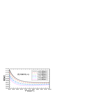
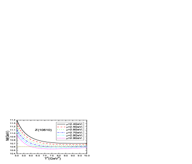
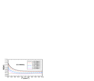
Figure 1: The masses with variations of the Borel parameters $T^{2}$ and energy scales $\mu$, where the horizontal lines denote the experimental values, the $Z(10610,+)$ denotes the positive charge conjugation partner of the $Z_{b}(10610)$.

In Fig.1, the masses are plotted with variations of the Borel parameters $T^{2}$ and energy scales $\mu$ for the threshold parameters $s_{0}=124\,\rm{GeV}^{2}$ and $s_{0}=125\,\rm{GeV}^{2}$ in the cases of the type I and type II tetraquark states, respectively. From the figure, we can see that the masses decrease monotonously with increase of the energy scales, just like that of the hidden charmed tetraquark states [14, 15, 16]. The energy scale $\mu=2.7\,\rm{GeV}$ is the optimal energy scale to reproduce the experimental value $M_{Z_{b}(10610)}=10.61\,\rm{GeV}$, then we can fit the parameter ${\mathbb{M}}_{b}=5.13\,\rm{GeV}$. The resulting energy scale $\mu=\sqrt{M^{2}_{Z_{b}(10650)}-(2\times 5.13\,\rm{GeV})^{2}}=2.85\,\rm{GeV}$ is the optimal energy scale to reproduce the experimental data $M_{Z_{b}(10650)}=10.65\,\rm{GeV}$ approximately. The energy scales $\mu=(2.8-2.9)\,\rm{GeV}$ are the allowed energy scales for the $Z_{b}(10650)$, see Fig.1; the uncertainty of the energy scale $\mu$ is about $0.05\,\rm{GeV}$. In this article, we take $\delta\mu=0.05\,\rm{GeV}$ for all the hidden bottom tetraquark states. The energy scale formula $\mu=\sqrt{M^{2}_{X/Y/Z}-(2{\mathbb{M}}_{Q})^{2}}$ works well, it also works well for the heavy molecular states [27], the results will be presented elsewhere.

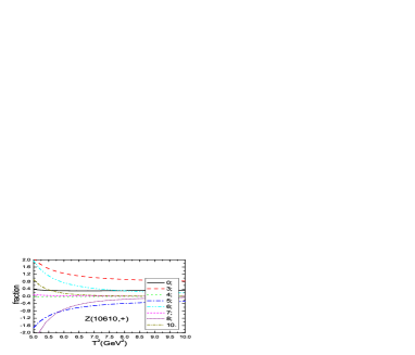
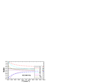
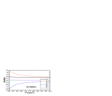
Figure 2: The contributions of different terms in the operator product expansion with variations of the Borel parameters $T^{2}$, where the 0, 3, 4, 5, 6, 7, 8, 10 denote the dimensions of the vacuum condensates, the $Z(10610,+)$ denotes the positive charge conjugation partner of the $Z_{b}(10610)$.

In Fig.2, the contributions of different terms in the operator product expansion are plotted with variations of the Borel parameters $T^{2}$ for the parameters $s_{0}=124\,\rm{GeV}^{2}$, $\mu=2.70\,\rm{GeV}$ and $s_{0}=125\,\rm{GeV}^{2}$, $\mu=2.85\,\rm{GeV}$ in the cases of the type I and type II tetraquark states, respectively. If we take the values $T^{2}=(7-8)\,\rm{GeV}^{2}$, the convergent behavior is very good. In Fig.3, the contributions of the pole terms are plotted with variations of the threshold parameters $s_{0}$ and Borel parameters $T^{2}$ at the energy scales $\mu=2.70\,\rm{GeV}$ and $\mu=2.85\,\rm{GeV}$ for the type I and type II tetraquark states, respectively. The values $T^{2}=(7-8)\,\rm{GeV}^{2}$ also lead to analogous pole contributions $(50-70)\%$. The pole dominance condition is also well satisfied. In Fig.3, the pole contributions are defined by

$${\rm pole} = \frac{\int_{4m_{b}^{2}}^{s_{0}}ds\,\rho(s)\exp\left(-\frac{s}{T^{2}}\right)}{\int_{4m_{b}^{2}}^{\infty}ds\,\rho(s)\exp\left(-\frac{s}{T^{2}}\right)}\,\,.$$ (16)

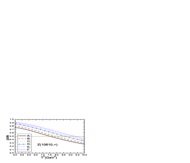
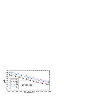
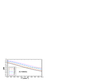
Figure 3: The pole contributions with variations of the Borel parameters $T^{2}$ and threshold parameters $s_{0}$, where the $A$, $B$, $C$, $D$, $E$, $F$ denote the threshold parameters $s_{0}=120$, $122$, $124$, $126$, $128$, $130\,\rm{GeV}^{2}$ respectively for the type I tetraquark states; $s_{0}=121$, $123$, $125$, $127$, $129$, $131\,\rm{GeV}^{2}$ respectively for the type II tetraquark states; the $Z(10610,+)$ denotes the positive charge conjugation partner of the $Z_{b}(10610)$.

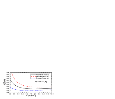
Figure 4: The masses with variations of the Borel parameters $T^{2}$, where the horizontal lines denote the experimental values, the $Z(10610,+)$ denotes the positive charge conjugation partner of the $Z_{b}(10610)$.

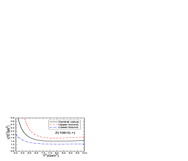
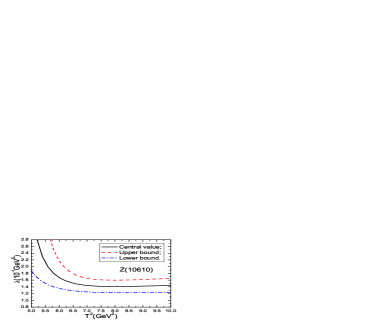
Figure 5: The pole residues with variations of the Borel parameters $T^{2}$, where the $Z(10610,+)$ denotes the positive charge conjugation partner of the $Z_{b}(10610)$.

We take into account all uncertainties of the input parameters (including the vacuum condensates, the $b$-quark mass, the continuum threshold parameter, the energy scale and the Borel parameter) and obtain the values of the masses and pole residues of the axial-vector hidden bottom tetraquark states, which are shown explicitly in Figs.4-5 and Table 1. In this article, we calculate the uncertainties $\delta$ with the formula,

$$\delta=\sqrt{\sum_{i}\left(\frac{\partial f}{\partial x_{i}}\right)^{2}\mid_{x_{i}=\bar{x}_{i}}(x_{i}-\bar{x}_{i})^{2}}\,,$$ (17)

where the $f$ denotes the masses and pole residues of the tetraquark states, the $x_{i}$ denote the input parameters $s_{0}$, $T^{2}$, $\mu$, $m_{b}$, $\langle\bar{q}q\rangle$, $\langle\bar{q}g_{s}\sigma Gq\rangle$, $\cdots$. As the partial derivatives $\frac{\partial f}{\partial x_{i}}$ are difficult to carry out analytically, we take the approximation $\left(\frac{\partial f}{\partial x_{i}}\right)^{2}(x_{i}-\bar{x}_{i})^{2}\approx\left[f(\bar{x}_{i}\pm\Delta x_{i})-f(\bar{x}_{i})\right]^{2}$ in numerical calculations with $x_{i}=\bar{x}_{i}\pm\Delta x_{i}$. From Table 1, we can see that the uncertainties of the masses $M_{Z}$ are about $1\%$, while the uncertainties of the pole residues $\lambda_{Z}$ are about $15\%$. We obtain the squared masses $M_{Z}^{2}$ through a fraction, see Eq.(13), the uncertainties in the numerator and denominator which originate from a given input parameter (for example, $\langle\bar{q}q\rangle$) cancel out with each other, and result in small net uncertainty.

$J^{PC}$	$T^{2}(\rm{GeV}^{2})$	$s_{0}(\rm{GeV}^{2})$	pole	$M_{Z}(\rm{GeV})$	$\lambda_{Z}$
$1^{++}$	$7-8$	$124\pm 2$	$(49-69)\%$	$10.60^{+0.12}_{-0.09}$	$1.40^{+0.23}_{-0.18}\times 10^{-1}\rm{GeV}^{5}$
$1^{+-}$ ($Z_{b}(10610)$)	$7-8$	$124\pm 2$	$(48-68)\%$	$10.61^{+0.13}_{-0.09}$	$1.42^{+0.24}_{-0.19}\times 10^{-1}\rm{GeV}^{5}$
$1^{+-}$ ($Z_{b}(10650)$)	$7-8$	$125\pm 2$	$(50-70)\%$	$10.64^{+0.09}_{-0.08}$	$1.72^{+0.24}_{-0.22}\times 10^{-2}\rm{GeV}^{4}$

Table 1: The Borel parameters, continuum threshold parameters, pole contributions, masses and pole residues of the axial-vector tetraquark states.

The present predictions $M_{Z_{b}(10610)}=\left(10.61^{+0.11}_{-0.09}\right)\,\rm{GeV}$ and $M_{Z_{b}(10650)}=\left(10.64^{+0.08}_{-0.08}\right)\,\rm{GeV}$ are consistent with the experimental values $M_{Z_{b}(10610)}=\left(10607.2\pm 2.0\right)\,\rm{MeV}$ and $M_{Z_{b}(10650)}=\left(10652.2\pm 1.5\right)\,\rm{MeV}$ [2]. The predicted masses favor assigning the $Z_{b}(10610)$ and $Z_{b}(10650)$ as the $1^{+-}$ type I and type II tetraquark states, respectively. There is no candidate experimentally for the $J^{PC}=1^{++}$ hidden bottom tetraquark states at the present time, the prediction $M_{Z}=\left(10.60^{+0.11}_{-0.09}\right)\,\rm{GeV}$ can be confronted with the experimental data in the future at the LHCb and Belle-II. The $C=+$ and $C=-$ type I axial-vector hidden bottom tetraquark states have degenerate masses from the QCD sum rules.

In the following, we perform Fierz re-arrangement to the axial-vector currents both in the color and Dirac-spinor spaces to obtain the results,

$$J_{1^{+-}}^{\mu} = \frac{\epsilon^{ijk}\epsilon^{imn}}{\sqrt{2}}\left\{u^{j}C\gamma_{5}b^{k}\bar{d}^{m}\gamma^{\mu}C\bar{b}^{n}-u^{j}C\gamma^{\mu}b^{k}\bar{d}^{m}\gamma_{5}C\bar{b}^{n}\right\}\,,$$ (18)

$$= \frac{1}{2\sqrt{2}}\left\{\,i\bar{b}i\gamma_{5}b\,\bar{d}\gamma^{\mu}u-i\bar{b}\gamma^{\mu}b\,\bar{d}i\gamma_{5}u+\bar{b}u\,\bar{d}\gamma^{\mu}\gamma_{5}b-\bar{b}\gamma^{\mu}\gamma_{5}u\,\bar{d}b\right.$$

$$\left.-i\bar{b}\gamma_{\nu}\gamma_{5}b\,\bar{d}\sigma^{\mu\nu}u+i\bar{b}\sigma^{\mu\nu}b\,\bar{d}\gamma_{\nu}\gamma_{5}u-i\bar{b}\sigma^{\mu\nu}\gamma_{5}u\,\bar{d}\gamma_{\nu}b+i\bar{b}\gamma_{\nu}u\,\bar{d}\sigma^{\mu\nu}\gamma_{5}b\,\right\}\,,$$

$$J_{1^{+-}}^{\mu\nu} = \frac{\epsilon^{ijk}\epsilon^{imn}}{\sqrt{2}}\left\{u^{j}C\gamma^{\mu}b^{k}\bar{d}^{m}\gamma^{\nu}C\bar{b}^{n}-u^{j}C\gamma^{\nu}b^{k}\bar{d}^{m}\gamma^{\mu}C\bar{b}^{n}\right\}\,,$$ (19)

$$= \frac{1}{2\sqrt{2}}\left\{\,i\bar{d}u\,\bar{b}\sigma^{\mu\nu}b+i\bar{d}\sigma^{\mu\nu}u\,\bar{b}b+i\bar{d}b\,\bar{b}\sigma^{\mu\nu}u+i\bar{d}\sigma^{\mu\nu}b\,\bar{b}u\right.$$

$$-\bar{b}\sigma^{\mu\nu}\gamma_{5}b\,\bar{d}i\gamma_{5}u-\bar{b}i\gamma_{5}b\,\bar{d}\sigma^{\mu\nu}\gamma_{5}u-\bar{b}\sigma^{\mu\nu}\gamma_{5}u\,\bar{d}i\gamma_{5}b-\bar{d}i\gamma_{5}b\,\bar{b}\sigma^{\mu\nu}\gamma_{5}u$$

$$+i\epsilon^{\mu\nu\alpha\beta}\bar{b}\gamma^{\alpha}\gamma_{5}b\,\bar{d}\gamma^{\beta}u-i\epsilon^{\mu\nu\alpha\beta}\bar{b}\gamma^{\alpha}b\,\bar{d}\gamma^{\beta}\gamma_{5}u$$

$$\left.+i\epsilon^{\mu\nu\alpha\beta}\bar{b}\gamma^{\alpha}\gamma_{5}u\,\bar{d}\gamma^{\beta}b-i\epsilon^{\mu\nu\alpha\beta}\bar{b}\gamma^{\alpha}u\,\bar{d}\gamma^{\beta}\gamma_{5}b\,\right\}\,,$$

$$J_{1^{++}}^{\mu} = \frac{\epsilon^{ijk}\epsilon^{imn}}{\sqrt{2}}\left\{u^{j}C\gamma_{5}b^{k}\bar{d}^{m}\gamma^{\mu}C\bar{b}^{n}+u^{j}C\gamma^{\mu}b^{k}\bar{d}^{m}\gamma_{5}C\bar{b}^{n}\right\}\,,$$ (20)

$$= \frac{1}{2\sqrt{2}}\left\{\,\bar{b}\gamma^{\mu}\gamma_{5}b\,\bar{d}u-\bar{b}b\,\bar{d}\gamma^{\mu}\gamma_{5}u+i\bar{b}\gamma^{\mu}u\,\bar{d}i\gamma_{5}b-i\bar{b}i\gamma_{5}u\,\bar{d}\gamma^{\mu}b\right.$$

$$\left.-i\bar{b}\gamma_{\nu}b\,\bar{d}\sigma^{\mu\nu}\gamma_{5}u+i\bar{b}\sigma^{\mu\nu}\gamma_{5}b\,\bar{d}\gamma_{\nu}u-i\bar{b}\sigma^{\mu\nu}u\,\bar{d}\gamma_{\nu}\gamma_{5}b+i\bar{b}\gamma_{\nu}\gamma_{5}u\,\bar{d}\sigma^{\mu\nu}b\,\right\}\,,$$

where we add the subscripts $1^{+-}$ and $1^{++}$ to denote the $J^{PC}$ explicitly. Then we obtain the Okubo-Zweig-Iizuka super-allowed strong decays by taking into account the couplings to the meson-meson pairs,

$$Z^{\pm}_{b}(10610)(1^{+-}) \to h_{b}({\rm 1P,2P})\pi^{\pm}\,,\,\Upsilon({\rm 1S,2S,3S})\pi^{\pm}\,,\,\eta_{b}({\rm 1S})\rho^{\pm}\,,\,\eta_{b}({\rm 1S,2S})(\pi\pi)_{\rm P}^{\pm}\,,$$

$$Z^{\pm}_{b}(10650)(1^{+-}) \to \Upsilon({\rm 1S,2S,3S})\pi^{\pm}\,,\,\eta_{b}({\rm 1S})\rho^{\pm}\,,\,\eta_{b}({\rm 1S,2S})(\pi\pi)_{\rm P}^{\pm}\,,\,\chi_{b1}({\rm 1P,2P})(\pi\pi)_{\rm P}^{\pm}\,,\,(B\bar{B}^{*})^{\pm}\,,$$

$$Z^{\pm}_{b}(10600)(1^{++}) \to \chi_{b0}({\rm 1P,2P})\pi^{\pm}\,,\,\Upsilon({\rm 1S})\rho^{\pm}\,,\,\Upsilon({\rm 1S,2S})(\pi\pi)_{\rm P}^{\pm}\,,$$ (21)

where we use the $(\pi\pi)_{\rm P}$ to denote the P-wave $\pi\pi$ systems have the same quantum numbers of the $\rho$, and take the decays to the $(\pi\pi)_{\rm P}^{\pm}$ final states as Okubo-Zweig-Iizuka super-allowed according to the decays $\rho\to\pi\pi$. In this article, we denote the hidden bottom tetraquark states with the mass $10600\,\rm{MeV}$ as the $Z_{b}(10600)$, see Table 1. We can search for the $Z^{\pm}_{b}(10650)(1^{+-})$ in the typical decays,

$$Z^{\pm}_{b}(10650)(1^{+-}) \to \chi_{b1}({\rm 1P,2P})(\pi\pi)_{\rm P}^{\pm}\,,\,(B\bar{B}^{*})^{\pm}\,,$$ (22)

which originate from the typical sub-structures of the $Z^{\pm}_{b}(10650)(1^{+-})$.

In the nonrelativistic and heavy quark limit, the components $\bar{b}\sigma^{\mu\nu}\gamma_{5}u\,\bar{d}\gamma_{\nu}b$ and $\epsilon^{\mu\nu\alpha\beta}\bar{b}\gamma^{\alpha}\gamma_{5}u\,\bar{d}\gamma^{\beta}b$ of the interpolating currents $J_{1^{+-}}^{\mu}$ and $J_{1^{+-}}^{\mu\nu}$ respectively are reduced to the following forms,

$$\bar{b}\sigma^{0j}\gamma_{5}u\,\bar{d}\gamma_{j}b \propto \xi^{\dagger}_{b}\sigma^{j}\zeta_{u}\,\chi^{\dagger}_{d}\vec{\sigma}\cdot\vec{k}_{d}\sigma^{j}\xi_{b}\,\,\,\propto\,\,\,\xi^{\dagger}_{b}\frac{\sigma^{j}}{2}\zeta_{u}\,\chi^{\dagger}_{d}\frac{\sigma^{j}}{2}\xi_{b}=\vec{S}_{B^{*}}\cdot\vec{S}_{\bar{B}^{*}}\,,$$

$$\bar{b}\sigma^{ij}\gamma_{5}u\,\bar{d}\gamma_{j}b \propto \epsilon^{ijk}\xi^{\dagger}_{b}\sigma^{k}\vec{\sigma}\cdot\vec{k}_{u}\zeta_{u}\,\chi^{\dagger}_{d}\vec{\sigma}\cdot\vec{k}_{d}\sigma^{j}\xi_{b}\,\,\,\propto\,\,\,\epsilon^{ijk}\xi^{\dagger}_{b}\frac{\sigma^{k}}{2}\zeta_{u}\,\chi^{\dagger}_{d}\frac{\sigma^{j}}{2}\xi_{b}=\vec{S}_{\bar{B}^{*}}\times\vec{S}_{B^{*}}\,,$$

$$\epsilon^{ijk}\bar{b}\gamma^{j}\gamma_{5}u\,\bar{d}\gamma^{k}b \propto \epsilon^{ijk}\xi^{\dagger}_{b}\sigma^{j}\zeta_{u}\,\chi^{\dagger}_{d}\vec{\sigma}\cdot\vec{k}_{d}\sigma^{k}\xi_{b}\,\,\,\propto\,\,\,\epsilon^{ijk}\xi^{\dagger}_{b}\frac{\sigma^{j}}{2}\zeta_{u}\,\chi^{\dagger}_{d}\frac{\sigma^{k}}{2}\xi_{b}=\vec{S}_{B_{1}}\times\vec{S}_{\bar{B}^{*}}\,,$$

$$\epsilon^{ijk}\bar{b}\gamma^{0}\gamma_{5}u\,\bar{d}\gamma^{k}b \propto \epsilon^{ijk}\xi^{\dagger}_{b}\vec{\sigma}\cdot\vec{k}_{u}\zeta_{u}\,\chi^{\dagger}_{d}\vec{\sigma}\cdot\vec{k}_{d}\sigma^{k}\xi_{b}\,\,\,\propto\,\,\,\epsilon^{ijk}\xi^{\dagger}_{b}\zeta_{u}\,\chi^{\dagger}_{d}\frac{\sigma^{k}}{2}\xi_{b}=\epsilon^{ijk}S^{k}_{\bar{B}^{*}}\,,$$ (23)

where the $\xi$, $\zeta$, $\chi$ are the two-component spinors of the quark fields, the $\vec{k}$ are the three-vectors of the quark fields, the $\sigma^{i}$ are the pauli matrixes, and the $\vec{S}$ are the spin operators. The thresholds are $B^{*}\bar{B}^{*}=10650\,\rm{MeV}$, $B\bar{B}^{*}=10605\,\rm{MeV}$, $B_{0}\bar{B}^{*}\approx B_{1}\bar{B}^{*}=11049\,\rm{MeV}$ [24]. It is obvious that the currents $\bar{b}\sigma^{\mu\nu}\gamma_{5}u\,\bar{d}\gamma_{\nu}b$ and $\bar{b}\gamma_{\nu}u\,\bar{d}\sigma^{\mu\nu}\gamma_{5}b$ ($\epsilon^{\mu\nu\alpha\beta}\bar{b}\gamma^{\alpha}\gamma_{5}u\,\bar{d}\gamma^{\beta}b$ and $\epsilon^{\mu\nu\alpha\beta}\bar{b}\gamma^{\alpha}u\,\bar{d}\gamma^{\beta}\gamma_{5}b$) couple to the $J^{P}=0^{+}$ and $1^{+}$ $(B^{*}\bar{B}^{*})^{+}$ ($J^{P}=1^{+}$ $(B_{1}^{*}\bar{B}^{*})^{+}$ and $(B_{0}^{*}\bar{B}^{*})^{+}$) states. The strong decays

$$Z^{\pm}_{b}(10610)(1^{+-}) \to (B^{*}\bar{B}^{*})^{\pm}\,,$$

$$Z^{\pm}_{b}(10650)(1^{+-}) \to (B_{1}\bar{B}^{*})^{\pm}\,,$$ (24)

are Okubo-Zweig-Iizuka super-allowed but kinematically forbidden. The $Z^{\pm}_{b}(10610)$ and $Z^{\pm}_{b}(10650)$ have the same quantum numbers and analogous strong decays but different masses and quark configurations.

Now we list out the possible strong decays of the $Z^{\pm}_{b}(10610)$, $Z^{\pm}_{b}(10650)$ and $Z_{b}^{\pm}(10600)$,

$$Z^{\pm}_{b}(10610)(1^{+-}) \to h_{b}({\rm 1P,2P})\pi^{\pm}\,,\,\Upsilon({\rm 1S,2S,3S})\pi^{\pm}\,,\,\eta_{b}({\rm 1S})\rho^{\pm}\,,\,\eta_{b}({\rm 1S,2S})(\pi\pi)_{\rm P}^{\pm}\,,\,$$

$$\chi_{b1}({\rm 1P,2P})(\pi\pi)_{\rm P}^{\pm}\,,$$

$$Z^{\pm}_{b}(10650)(1^{+-}) \to h_{b}({\rm 1P,2P})\pi^{\pm}\,,\,\Upsilon({\rm 1S,2S,3S})\pi^{\pm}\,,\,\eta_{b}({\rm 1S})\rho^{\pm}\,,\,\eta_{b}({\rm 1S,2S})(\pi\pi)_{\rm P}^{\pm}\,,\,$$

$$\chi_{b1}({\rm 1P,2P})(\pi\pi)_{\rm P}^{\pm}\,,\,(B\bar{B}^{*})^{\pm}\,,\,(B^{*}{\bar{B}}^{*})^{\pm}\,,$$

$$Z^{\pm}_{b}(10600)(1^{++}) \to \chi_{b0}({\rm 1P,2P})\pi^{\pm}\,,\,\chi_{b1}({\rm 1P,2P})\pi^{\pm}\,,\,\Upsilon({\rm 1S})\rho^{\pm}\,,\,\Upsilon({\rm 1S,2S})(\pi\pi)_{\rm P}^{\pm}\,.$$ (25)

The following strong decays take place through the re-scattering mechanism,

$$Z^{\pm}_{b}(10610)(1^{+-}) \to \chi_{b1}({\rm 1P,2P})(\pi\pi)_{\rm P}^{\pm}\,,$$

$$Z^{\pm}_{b}(10650)(1^{+-}) \to h_{b}({\rm 1P,2P})\pi^{\pm}\,,\,(B^{*}{\bar{B}}^{*})^{\pm}\,,$$

$$Z^{\pm}_{b}(10600)(1^{++}) \to \chi_{b1}({\rm 1P,2P})\pi^{\pm}\,,$$ (26)

and cannot be the dominant decay modes.

We can also search for the neutral partner $Z^{0}_{b}(10610/10650)(1^{+-})$ in the following strong and electromagnetic decays,

$$Z^{0}_{b}(10610/10650)(1^{+-}) \to h_{c}({\rm 1P,2P})\pi^{0}\,,\,\Upsilon({\rm 1S,2S,3S})\pi^{0}\,,\,\eta_{b}({\rm 1S})\rho^{0}\,,\,\eta_{b}({\rm 1S})\omega\,,\,\eta_{b}({\rm 1S,2S})(\pi\pi)_{\rm P}^{0}\,,\,$$ (27)

$$\chi_{bj}({\rm 1P,2P})(\pi\pi)_{\rm P}^{0}\,,\,\eta_{b}({\rm 1S,2S})(\pi\pi\pi)_{\rm P}^{0}\,,\,\chi_{bj}({\rm 1P})(\pi\pi\pi)_{\rm P}^{0}\,,\,\eta_{b}({\rm 1S,2S})\gamma\,,\,$$

$$\chi_{bj}({\rm 1P,2P})\gamma\,,\,(B\bar{B}^{*})^{0}\,,$$

where the $(\pi\pi\pi)_{\rm P}$ denotes the P-wave $\pi\pi\pi$ systems with the same quantum numbers of the $\omega$.

The diquark-antidiquark type current with special quantum numbers couples to a special tetraquark state, while the current can be re-arranged both in the color and Dirac-spinor spaces, and changed to a current as a special superposition of color singlet-singlet type currents. The color singlet-singlet type currents couple to the meson-meson pairs. The diquark-antidiquark type tetraquark state can be taken as a special superposition of a series of meson-meson pairs, and embodies the net effects. The decays to its components (meson-meson pairs) are Okubo-Zweig-Iizuka super-allowed, but the re-arrangements in the color-space are non-trivial [28].

4 Strong decays $Z_{b}^{\pm}(10610)\to\Upsilon\pi^{\pm},\,\,\eta_{b}\rho^{\pm}$

The pole residues $\lambda_{Z_{b}}$ can be taken as basic input parameters to study relevant processes of the axial-vector tetraquark states $Z^{\pm}_{b}(10610)$, $Z^{\pm}_{b}(10650)$ and $Z_{b}^{\pm}(10600)$ with the three-point QCD sum rules. For example, we can study the strong decays $Z_{b}^{\pm}(10610)\to\Upsilon\pi^{\pm}$ and $\eta_{b}\rho^{\pm}$ with the following three-point correlation functions $\Pi_{\mu,\nu}^{1}(p,q)$ and $\Pi_{\mu,\nu}^{2}(p,q)$, respectively,

$$\Pi_{\mu,\nu}^{1}(p,q) = i^{2}\int d^{4}xd^{4}ye^{ipx}e^{iqy}\langle 0|T\left\{J_{\mu}^{\Upsilon}(x)J_{5}^{\pi}(y)J_{\nu,1^{+-}}(0)\right\}|0\rangle\,,$$

$$\Pi_{\mu,\nu}^{2}(p,q) = i^{2}\int d^{4}xd^{4}ye^{ipx}e^{iqy}\langle 0|T\left\{J_{5}^{\eta_{b}}(x)J_{\mu}^{\rho}(y)J_{\nu,1^{+-}}(0)\right\}|0\rangle\,,$$ (28)

where the currents

$$J_{\mu}^{\Upsilon}(x) = \bar{b}(x)\gamma_{\mu}b(x)\,,$$

$$J_{\mu}^{\rho}(y) = \bar{u}(y)\gamma_{\mu}d(y)\,,$$

$$J_{5}^{\eta_{b}}(x) = \bar{b}(x)i\gamma_{5}b(x)\,,$$

$$J_{5}^{\pi}(y) = \bar{u}(y)i\gamma_{5}d(y)\,,$$ (29)

interpolate the mesons $\Upsilon$, $\rho$, $\eta_{b}$, $\pi$, respectively.

We insert a complete set of intermediate hadronic states with the same quantum numbers as the current operators into the three-point correlation functions and isolate the ground state contributions to obtain the following results,

$$\Pi_{\mu,\nu}^{1}(p,q) = \frac{f_{\pi}M_{\pi}^{2}f_{\Upsilon}M_{\Upsilon}\lambda_{Z_{b}}G_{Z_{b}\Upsilon\pi}}{m_{u}+m_{d}}\frac{-i}{(M_{Z_{b}}^{2}-p^{\prime 2})(M_{\Upsilon}^{2}-p^{2})(M_{\pi}^{2}-q^{2})}\left(-g_{\mu\alpha}+\frac{p_{\mu}p_{\alpha}}{p^{2}}\right)$$

$$\left(-g_{\nu}^{\alpha}+\frac{p^{\prime}_{\nu}p^{\prime\alpha}}{p^{\prime 2}}\right)+\cdots\,,$$

$$\Pi_{\mu,\nu}^{2}(p,q) = \frac{f_{\eta_{b}}M_{\eta_{b}}^{2}f_{\rho}M_{\rho}\lambda_{Z_{b}}G_{Z_{b}\eta_{b}\rho}}{2m_{b}}\frac{-i}{(M_{Z_{b}}^{2}-p^{\prime 2})(M_{\eta_{b}}^{2}-p^{2})(M_{\rho}^{2}-q^{2})}\left(-g_{\mu\alpha}+\frac{q_{\mu}q_{\alpha}}{q^{2}}\right)$$ (30)

$$\left(-g_{\nu}^{\alpha}+\frac{p^{\prime}_{\nu}p^{\prime\alpha}}{p^{\prime 2}}\right)+\cdots\,,$$

where $p^{\prime}=p+q$, the $f_{\Upsilon}$, $f_{\eta_{b}}$, $f_{\rho}$ and $f_{\pi}$ are the decay constants of the mesons $\Upsilon$, $\eta_{b}$, $\rho$ and $\pi$, respectively, the $G_{Z_{b}\Upsilon\pi}$ and $G_{Z_{b}\eta_{b}\rho}$ are the hadronic coupling constants. In the following, we write down the definitions,

$$\langle 0|J_{\mu}^{\Upsilon}(0)|\Upsilon(p)\rangle = f_{\Upsilon}M_{\Upsilon}\xi_{\mu}\,\,,$$

$$\langle 0|J_{\mu}^{\rho}(0)|\rho(q)\rangle = f_{\rho}M_{\rho}\varepsilon_{\mu}\,\,,$$

$$\langle 0|J_{5}^{\eta_{b}}(0)|\eta_{b}(p)\rangle = \frac{f_{\eta_{b}}M_{\eta_{b}}^{2}}{2m_{b}}\,\,,$$

$$\langle 0|J_{5}^{\pi}(0)|\pi(q)\rangle = \frac{f_{\pi}M_{\pi}^{2}}{m_{u}+m_{d}}\,\,,$$

$$\langle\Upsilon(p)\pi(q)|Z_{b}(p^{\prime})\rangle = \xi^{*}(p)\cdot\zeta(p^{\prime})G_{Z_{b}\Upsilon\pi}(q^{2})\,,$$

$$\langle\eta_{b}(p)\rho(q)|Z_{b}(p^{\prime})\rangle = \varepsilon^{*}(q)\cdot\zeta(p^{\prime})G_{Z_{b}\eta_{b}\rho}(q^{2})\,,$$ (31)

the $\xi$, $\zeta$ and $\varepsilon$ are polarization vectors of the $\Upsilon$, $Z_{b}$ and $\rho$, respectively. Now we choose the tensors $q_{\mu}p_{\nu}$ and $p_{\mu}q_{\nu}$ to study the coupling constants $G_{Z_{b}\Upsilon\pi}$ and $G_{Z_{b}\eta_{b}\rho}$, respectively. We carry out the operator product expansion and take into account the color connected Feynman diagrams [28],

$$\Pi^{1}_{\mu\nu}(p,q) = \frac{im_{b}\langle\bar{q}g_{s}\sigma Gq\rangle q_{\mu}p_{\nu}}{48\sqrt{2}\pi^{2}q^{2}}\int_{0}^{1}dx\frac{1}{x(1-x)p^{2}-m_{b}^{2}}$$ (32)

$$+\frac{ig_{s}^{2}\langle\bar{q}q\rangle^{2}q_{\mu}p_{\nu}}{81\sqrt{2}\pi^{2}q^{2}}\int_{0}^{1}dx\left\{\frac{3}{2\left[x(1-x)p^{2}-m_{b}^{2}\right]}+\frac{3x(1-x)m_{b}^{2}}{2\left[x(1-x)p^{2}-m_{b}^{2}\right]^{2}}\right.$$

$$\left.-\frac{4x(1-x)}{x(1-x)p^{2}-m_{b}^{2}}-\frac{\left[x^{2}+(1-x)^{2}\right]m_{b}^{2}}{\left[x(1-x)p^{2}-m_{b}^{2}\right]^{2}}\right\}\,,$$

$$\Pi^{2}_{\mu\nu}(p,q) = -\frac{im_{b}\langle\bar{q}g_{s}\sigma Gq\rangle p_{\mu}q_{\nu}}{48\sqrt{2}\pi^{2}q^{2}}\int_{0}^{1}dx\frac{1}{x(1-x)p^{2}-m_{b}^{2}}$$ (33)

$$-\frac{ig_{s}^{2}\langle\bar{q}q\rangle^{2}p_{\mu}q_{\nu}}{81\sqrt{2}\pi^{2}q^{2}}\int_{0}^{1}dx\left\{\frac{3}{2\left[x(1-x)p^{2}-m_{b}^{2}\right]}+\frac{3x(1-x)m_{b}^{2}}{2\left[x(1-x)p^{2}-m_{b}^{2}\right]^{2}}\right.$$

$$\left.-\frac{4x(1-x)}{x(1-x)p^{2}-m_{b}^{2}}-\frac{\left[x^{2}+(1-x)^{2}\right]m_{b}^{2}}{\left[x(1-x)p^{2}-m_{b}^{2}\right]^{2}}\right\}\,.$$

Then we take the Borel transform with respect to the variable $P^{2}=-p^{2}=-p^{\prime 2}$ and obtain the following QCD sum rules,

$$\frac{f_{\pi}M_{\pi}^{2}f_{\Upsilon}M_{\Upsilon}\lambda_{Z_{b}}G_{Z_{b}\Upsilon\pi}}{(m_{u}+m_{d})M_{Z_{b}}^{2}(M_{Z_{b}}^{2}-M_{\Upsilon}^{2})}\left\{\exp\left(-\frac{M_{\Upsilon}^{2}}{T^{2}}\right)-\exp\left(-\frac{M_{Z_{b}}^{2}}{T^{2}}\right)\right\}+C\exp\left(-\frac{s_{0}}{T^{2}}\right)$$

$$=\frac{m_{b}\langle\bar{q}g_{s}\sigma Gq\rangle}{48\sqrt{2}\pi^{2}}\frac{Q^{2}+M_{\pi}^{2}}{Q^{2}}\int_{0}^{1}dx\frac{1}{x(1-x)}\exp\left(-\frac{m_{b}^{2}}{x(1-x)T^{2}}\right)$$

$$+\frac{g_{s}^{2}\langle\bar{q}q\rangle^{2}}{81\sqrt{2}\pi^{2}}\frac{Q^{2}+M_{\pi}^{2}}{Q^{2}}\int_{0}^{1}dx\left\{\frac{3}{2x(1-x)}\left(1-\frac{m_{b}^{2}}{T^{2}}\right)-4\left[1-\left(\frac{1}{x^{2}}+\frac{1}{(1-x)^{2}}\right)\frac{m_{b}^{2}}{4T^{2}}\right]\right\}$$

$$\exp\left(-\frac{m_{b}^{2}}{x(1-x)T^{2}}\right)\,,$$ (34)

$$\frac{f_{\eta_{b}}M_{\eta_{b}}^{2}f_{\rho}M_{\rho}\lambda_{Z_{b}}G_{Z_{b}\eta_{b}\rho}}{2m_{b}M_{Z_{b}}^{2}(M_{Z_{b}}^{2}-M_{\eta_{b}}^{2})}\left\{\exp\left(-\frac{M_{\eta_{b}}^{2}}{T^{2}}\right)-\exp\left(-\frac{M_{Z_{b}}^{2}}{T^{2}}\right)\right\}+C\exp\left(-\frac{s_{0}}{T^{2}}\right)$$

$$=-\frac{m_{b}\langle\bar{q}g_{s}\sigma Gq\rangle}{48\sqrt{2}\pi^{2}}\frac{Q^{2}+M_{\rho}^{2}}{Q^{2}}\int_{0}^{1}dx\frac{1}{x(1-x)}\exp\left(-\frac{m_{b}^{2}}{x(1-x)T^{2}}\right)$$

$$-\frac{g_{s}^{2}\langle\bar{q}q\rangle^{2}}{81\sqrt{2}\pi^{2}}\frac{Q^{2}+M_{\rho}^{2}}{Q^{2}}\int_{0}^{1}dx\left\{\frac{3}{2x(1-x)}\left(1-\frac{m_{b}^{2}}{T^{2}}\right)-4\left[1-\left(\frac{1}{x^{2}}+\frac{1}{(1-x)^{2}}\right)\frac{m_{b}^{2}}{4T^{2}}\right]\right\}$$

$$\exp\left(-\frac{m_{b}^{2}}{x(1-x)T^{2}}\right)\,,$$ (35)

where the $s_{0}$ is the continuum threshold parameter for the $Z_{b}(10610)$, and the $C$ are unknown parameters introduced to take into account single-pole contributions associated with pole-continuum transitions. In the three-point QCD sum rules, the single-pole contributions are not suppressed if a single Borel transform is taken.

The input parameters are taken as $M_{\pi}=0.140\,\rm{GeV}$, $f_{\pi}=0.130\,\rm{GeV}$, $M_{\Upsilon}=9.4603\,\rm{GeV}$, $M_{\eta_{b}}=9.398\,\rm{GeV}$, $M_{\rho}=0.775\,\rm{GeV}$, $f_{\rho}=0.215\,\rm{GeV}$, $f_{\Upsilon}=f_{\eta_{b}}=0.700\,\rm{GeV}$ [24, 29], and $m_{u}({\mu=\rm 1GeV})=m_{d}({\mu=\rm 1GeV})=0.006\,\rm{GeV}$ from the Gell-Mann-Oakes-Renner relation. The unknown parameters are chosen as $C=0.0014\,\rm{GeV}^{6}$ and $-0.0010\,\rm{GeV}^{6}$ in the QCD sum rules for the coupling constants $G_{Z_{b}\Upsilon\pi}$ and $G_{Z_{b}\eta_{b}\rho}$ respectively to obtain platforms in the Borel windows $T^{2}=(7-8)\,\rm{GeV}^{2}$. The central values of the $G_{Z_{b}\Upsilon\pi}$ and $G_{Z_{b}\eta_{b}\rho}$ can be fitted to the following forms,

$$|G_{Z_{b}\Upsilon\pi}(Q^{2})| = 3.53\,\rm{GeV}\,,$$

$$G_{Z_{b}\eta_{b}\rho}(Q^{2}) = \frac{1421.9\,{\rm GeV^{3}}}{257.4\,{\rm GeV^{2}}+Q^{2}}\,,$$ (36)

with $Q^{2}=-q^{2}$. We extend the coupling constants to the physical regions and take into account the uncertainties,

$$|G_{Z_{b}\Upsilon\pi}\left(Q^{2}=-M_{\pi}^{2}\right)| = 3.53^{+1.21}_{-0.91}\,\rm{GeV}\,,$$

$$G_{Z_{b}\eta_{b}\rho}\left(Q^{2}=-M_{\rho}^{2}\right) = 5.54^{+1.82}_{-1.42}\,\rm{GeV}\,.$$ (37)

The resulting decay widths are

$$\Gamma(Z_{b}^{+}(10610)\to\Upsilon\pi^{+}) = \frac{p\left(M_{Z_{b}},M_{\Upsilon},M_{\pi}\right)}{24\pi M_{Z_{b}}^{2}}G_{Z_{b}\Upsilon\pi}^{2}\left(3+\frac{p\left(M_{Z_{b}},M_{\Upsilon},M_{\pi}\right)^{2}}{M_{\Upsilon}^{2}}\right)$$

$$= 4.77^{+3.27}_{-2.46}\,\rm{MeV}\,,$$

$$\Gamma(Z_{b}^{+}(10610)\to\eta_{b}\rho^{+}) = \frac{p\left(M_{Z_{b}},M_{\eta_{b}},M_{\rho}\right)}{24\pi M_{Z_{b}}^{2}}G_{Z_{b}\eta_{b}\rho}^{2}\left(3+\frac{p\left(M_{Z_{b}},M_{\eta_{b}},M_{\rho}\right)^{2}}{M_{\rho}^{2}}\right)$$ (38)

$$= 13.52^{+8.89}_{-6.93}\,\rm{MeV}\,,$$

where $p(a,b,c)=\frac{\sqrt{[a^{2}-(b+c)^{2}][a^{2}-(b-c)^{2}]}}{2a}$. Those widths are consistent with the experimental data $\Gamma_{Z_{b}(10610)}=(18.4\pm 2.4)\,\rm{MeV}$ from the Belle collaboration [2], the present calculations support assigning the $Z_{b}(10610)$ as the $1^{+-}$ diquark-antidiquark type tetraquark state. We can search for the $Z_{b}^{\pm}(10610)$ in the final states $\eta_{b}\rho^{\pm}$. The strong decays $Z^{\pm}_{b}(10610)(1^{+-})\to h_{b}({\rm 1P,2P})\pi^{\pm}$ take place through relative P-wave, the decay widths $\Gamma(Z^{\pm}_{b}(10610)(1^{+-})\to h_{b}({\rm 1P,2P})\pi^{\pm})\propto p\left(M_{Z_{b}},M_{h_{b}},M_{\pi}\right)^{3}$, and the decays are kinematically suppressed in the phase-space. Detailed studies based on the QCD sum rules are postponed to our next work.

5 Conclusion

In this article, we study the axial-vector mesons $Z_{b}(10610)$ and $Z_{b}(10650)$ with the $C\gamma_{\mu}-C\gamma_{5}$ type and $C\gamma_{\mu}-C\gamma_{\nu}$ type interpolating currents respectively by carrying out the operator product expansion to the vacuum condensates up to dimension-10. In calculations, we study the energy scale dependence of the QCD spectral densities in details for the first time, and suggest a formula $\mu=\sqrt{M^{2}_{X/Y/Z}-(2{\mathbb{M}}_{b})^{2}}$ with the effective mass ${\mathbb{M}}_{b}=5.13\,\rm{GeV}$ to determine the energy scales, which works very well. The numerical results support assigning the $Z_{b}(10610)$ and $Z_{b}(10650)$ as the $C\gamma_{\mu}-C\gamma_{5}$ type and $C\gamma_{\mu}-C\gamma_{\nu}$ type hidden bottom tetraquark states, respectively. The $Z_{b}(10610)$, $Z_{b}(10650)$, $Z_{c}(3900)$ and $Z_{c}(4020)$ are observed in the analogous decays to the final states $\pi^{\pm}\Upsilon({\rm 1,2,3S})$, $\pi^{\pm}h_{b}({\rm 1,2P})$, $\pi^{\pm}J/\psi$, $\pi^{\pm}h_{c}$, and should have analogous structures. Furthermore, we obtain the mass of the $C\gamma_{\mu}-C\gamma_{5}$ type $J^{PC}=1^{++}$ hidden bottom tetraquark state, which can be confronted with the experimental data in the future at the LHCb and Belle-II. The pole residues $\lambda_{Z_{b}}$ can be taken as basic input parameters to study relevant processes of the axial-vector tetraquark states $Z^{\pm}_{b}(10610)$, $Z^{\pm}_{b}(10650)$ and $Z_{b}^{\pm}(10600)$ with the three-point QCD sum rules. We study the strong decays $Z_{b}^{\pm}(10610)\to\Upsilon\pi^{\pm}\,,\,\eta_{b}\rho^{\pm}$ with the three-point QCD sum rules, the decay widths also support assigning the $Z_{b}(10610)$ as the $C\gamma_{\mu}-C\gamma_{5}$ type hidden bottom tetraquark state.

Appendix

The spectral densities at the level of the quark-gluon degrees of freedom,

$$\rho^{\rm I}_{0}(s) = \frac{1}{3072\pi^{6}}\int_{y_{i}}^{y_{f}}dy\int_{z_{i}}^{1-y}dz\,yz(1-y-z)^{3}\left(s-\overline{m}_{b}^{2}\right)^{2}\left(35s^{2}-26s\overline{m}_{b}^{2}+3\overline{m}_{b}^{2}\right)\,,$$ (39)

$$\rho^{\rm I}_{3}(s) = -\frac{m_{b}\langle\bar{q}q\rangle}{64\pi^{4}}\int_{y_{i}}^{y_{f}}dy\int_{z_{i}}^{1-y}dz\,(y+z)(1-y-z)\left(s-\overline{m}_{b}^{2}\right)\left(7s-3\overline{m}_{b}^{2}\right)\,,$$ (40)

$$\rho^{\rm I}_{4}(s) = -\frac{m_{b}^{2}}{2304\pi^{4}}\langle\frac{\alpha_{s}GG}{\pi}\rangle\int_{y_{i}}^{y_{f}}dy\int_{z_{i}}^{1-y}dz\left(\frac{z}{y^{2}}+\frac{y}{z^{2}}\right)(1-y-z)^{3}\left\{8s-3\overline{m}_{b}^{2}+\overline{m}_{b}^{4}\delta\left(s-\overline{m}_{b}^{2}\right)\right\}$$ (41)

$$+\frac{1}{1536\pi^{4}}\langle\frac{\alpha_{s}GG}{\pi}\rangle\int_{y_{i}}^{y_{f}}dy\int_{z_{i}}^{1-y}dz(y+z)(1-y-z)^{2}\,s\,(5s-4\overline{m}_{b}^{2})$$

$$-t\frac{m_{b}^{2}}{1152\pi^{4}}\langle\frac{\alpha_{s}GG}{\pi}\rangle\int_{y_{i}}^{y_{f}}dy\int_{z_{i}}^{1-y}dz\left(s-\overline{m}_{b}^{2}\right)\left\{1-\left(\frac{1}{y}+\frac{1}{z}\right)(1-y-z)\right.$$

$$\left.+\frac{(1-y-z)^{2}}{2yz}-\frac{1-y-z}{2}+\left(\frac{1}{y}+\frac{1}{z}\right)\frac{(1-y-z)^{2}}{4}-\frac{(1-y-z)^{3}}{12yz}\right\}\,,$$

$$\rho^{\rm I}_{5}(s) = \frac{m_{b}\langle\bar{q}g_{s}\sigma Gq\rangle}{128\pi^{4}}\int_{y_{i}}^{y_{f}}dy\int_{z_{i}}^{1-y}dz(y+z)\left(5s-3\overline{m}_{b}^{2}\right)$$ (42)

$$-\frac{m_{b}\langle\bar{q}g_{s}\sigma Gq\rangle}{128\pi^{4}}\int_{y_{i}}^{y_{f}}dy\int_{z_{i}}^{1-y}dz\left(\frac{y}{z}+\frac{z}{y}\right)(1-y-z)\left(2s-\overline{m}_{b}^{2}\right)$$

$$-t\frac{m_{b}\langle\bar{q}g_{s}\sigma Gq\rangle}{1152\pi^{4}}\int_{y_{i}}^{y_{f}}dy\int_{z_{i}}^{1-y}dz\left(\frac{y}{z}+\frac{z}{y}\right)(1-y-z)\left(5s-3\overline{m}_{b}^{2}\right)\,,$$

$$\rho^{\rm I}_{6}(s) = \frac{m_{b}^{2}\langle\bar{q}q\rangle^{2}}{12\pi^{2}}\int_{y_{i}}^{y_{f}}dy+\frac{g_{s}^{2}\langle\bar{q}q\rangle^{2}}{648\pi^{4}}\int_{y_{i}}^{y_{f}}dy\int_{z_{i}}^{1-y}dz\,yz\left\{8s-3\overline{m}_{b}^{2}+\overline{m}_{b}^{4}\delta\left(s-\overline{m}_{b}^{2}\right)\right\}$$ (43)

$$-\frac{g_{s}^{2}\langle\bar{q}q\rangle^{2}}{2592\pi^{4}}\int_{y_{i}}^{y_{f}}dy\int_{z_{i}}^{1-y}dz(1-y-z)\left\{\left(\frac{z}{y}+\frac{y}{z}\right)3\left(7s-4\overline{m}_{b}^{2}\right)\right.$$

$$\left.+\left(\frac{z}{y^{2}}+\frac{y}{z^{2}}\right)m_{b}^{2}\left[7+5\overline{m}_{b}^{2}\delta\left(s-\overline{m}_{b}^{2}\right)\right]-(y+z)\left(4s-3\overline{m}_{b}^{2}\right)\right\}$$

$$-\frac{g_{s}^{2}\langle\bar{q}q\rangle^{2}}{3888\pi^{4}}\int_{y_{i}}^{y_{f}}dy\int_{z_{i}}^{1-y}dz(1-y-z)\left\{\left(\frac{z}{y}+\frac{y}{z}\right)3\left(2s-\overline{m}_{b}^{2}\right)\right.$$

$$\left.+\left(\frac{z}{y^{2}}+\frac{y}{z^{2}}\right)m_{b}^{2}\left[1+\overline{m}_{b}^{2}\delta\left(s-\overline{m}_{b}^{2}\right)\right]+(y+z)2\left[8s-3\overline{m}_{b}^{2}+\overline{m}_{b}^{4}\delta\left(s-\overline{m}_{b}^{2}\right)\right]\right\}\,,$$

$$\rho^{\rm I}_{7}(s) = \frac{m_{b}^{3}\langle\bar{q}q\rangle}{576\pi^{2}}\langle\frac{\alpha_{s}GG}{\pi}\rangle\int_{y_{i}}^{y_{f}}dy\int_{z_{i}}^{1-y}dz\left(\frac{y}{z^{3}}+\frac{z}{y^{3}}+\frac{1}{y^{2}}+\frac{1}{z^{2}}\right)(1-y-z)$$ (44)

$$\left(1+\frac{2\overline{m}_{b}^{2}}{T^{2}}\right)\delta\left(s-\overline{m}_{b}^{2}\right)$$

$$-\frac{m_{b}\langle\bar{q}q\rangle}{64\pi^{2}}\langle\frac{\alpha_{s}GG}{\pi}\rangle\int_{y_{i}}^{y_{f}}dy\int_{z_{i}}^{1-y}dz\left(\frac{y}{z^{2}}+\frac{z}{y^{2}}\right)(1-y-z)\left\{1+\frac{2\overline{m}_{b}^{2}}{3}\delta\left(s-\overline{m}_{b}^{2}\right)\right\}$$

$$-\frac{m_{b}\langle\bar{q}q\rangle}{192\pi^{2}}\langle\frac{\alpha_{s}GG}{\pi}\rangle\int_{y_{i}}^{y_{f}}dy\int_{z_{i}}^{1-y}dz\left\{1+\frac{2\overline{m}_{b}^{2}}{3}\delta\left(s-\overline{m}_{b}^{2}\right)\right\}$$

$$-t\frac{m_{b}\langle\bar{q}q\rangle}{288\pi^{2}}\langle\frac{\alpha_{s}GG}{\pi}\rangle\int_{y_{i}}^{y_{f}}dy\int_{z_{i}}^{1-y}dz\left\{1-\left(\frac{1}{y}+\frac{1}{z}\right)\frac{1-y-z}{2}\right\}\left\{1+\frac{2\overline{m}_{b}^{2}}{3}\delta\left(s-\overline{m}_{b}^{2}\right)\right\}$$

$$-\frac{m_{b}\langle\bar{q}q\rangle}{384\pi^{2}}\langle\frac{\alpha_{s}GG}{\pi}\rangle\int_{y_{i}}^{y_{f}}dy\left\{1+\frac{2\widetilde{m}_{b}^{2}}{3}\delta\left(s-\widetilde{m}_{b}^{2}\right)\right\}\,,$$

$$\rho^{\rm I}_{8}(s) = -\frac{m_{b}^{2}\langle\bar{q}q\rangle\langle\bar{q}g_{s}\sigma Gq\rangle}{24\pi^{2}}\int_{0}^{1}dy\left(1+\frac{\widetilde{m}_{b}^{2}}{T^{2}}\right)\delta\left(s-\widetilde{m}_{b}^{2}\right)$$ (45)

$$+\frac{m_{b}^{2}\langle\bar{q}q\rangle\langle\bar{q}g_{s}\sigma Gq\rangle}{96\pi^{2}}\int_{0}^{1}dy\left(\frac{1}{y}+\frac{1}{1-y}\right)\delta\left(s-\widetilde{m}_{b}^{2}\right)$$

$$+t\frac{\langle\bar{q}q\rangle\langle\bar{q}g_{s}\sigma Gq\rangle}{288\pi^{2}}\int_{y_{i}}^{y_{f}}dy\left\{1+\frac{2\widetilde{m}_{b}^{2}}{3}\delta\left(s-\widetilde{m}_{b}^{2}\right)\right\}\,,$$

$$\rho^{\rm I}_{10}(s) = \frac{m_{b}^{2}\langle\bar{q}g_{s}\sigma Gq\rangle^{2}}{192\pi^{2}T^{6}}\int_{0}^{1}dy\widetilde{m}_{b}^{4}\delta\left(s-\widetilde{m}_{b}^{2}\right)$$ (46)

$$-\frac{m_{b}^{4}\langle\bar{q}q\rangle^{2}}{216T^{4}}\langle\frac{\alpha_{s}GG}{\pi}\rangle\int_{0}^{1}dy\left\{\frac{1}{y^{3}}+\frac{1}{(1-y)^{3}}\right\}\delta\left(s-\widetilde{m}_{b}^{2}\right)$$

$$+\frac{m_{b}^{2}\langle\bar{q}q\rangle^{2}}{72T^{2}}\langle\frac{\alpha_{s}GG}{\pi}\rangle\int_{0}^{1}dy\left\{\frac{1}{y^{2}}+\frac{1}{(1-y)^{2}}\right\}\delta\left(s-\widetilde{m}_{b}^{2}\right)$$

$$-t\frac{\langle\bar{q}q\rangle^{2}}{1296}\langle\frac{\alpha_{s}GG}{\pi}\rangle\int_{0}^{1}dy\left(1+\frac{2\widetilde{m}_{b}^{2}}{T^{2}}\right)\delta\left(s-\widetilde{m}_{b}^{2}\right)$$

$$-\frac{m_{b}^{2}\langle\bar{q}g_{s}\sigma Gq\rangle^{2}}{384\pi^{2}T^{4}}\int_{0}^{1}dy\left(\frac{1}{y}+\frac{1}{1-y}\right)\widetilde{m}_{b}^{2}\delta\left(s-\widetilde{m}_{b}^{2}\right)$$

$$-t\frac{\langle\bar{q}g_{s}\sigma Gq\rangle^{2}}{1728\pi^{2}}\int_{0}^{1}dy\left(1+\frac{3\widetilde{m}_{b}^{2}}{2T^{2}}+\frac{\widetilde{m}_{b}^{4}}{T^{4}}\right)\delta\left(s-\widetilde{m}_{b}^{2}\right)$$

$$-t\frac{\langle\bar{q}g_{s}\sigma Gq\rangle^{2}}{2304\pi^{2}}\int_{0}^{1}dy\left(1+\frac{2\widetilde{m}_{b}^{2}}{T^{2}}\right)\delta\left(s-\widetilde{m}_{b}^{2}\right)$$

$$+\frac{m_{b}^{2}\langle\bar{q}q\rangle^{2}}{216T^{6}}\langle\frac{\alpha_{s}GG}{\pi}\rangle\int_{0}^{1}dy\widetilde{m}_{b}^{4}\delta\left(s-\widetilde{m}_{b}^{2}\right)\,,$$

$$\rho^{\rm II}_{0}(s) = \frac{1}{3072\pi^{6}s}\int_{y_{i}}^{y_{f}}dy\int_{z_{i}}^{1-y}dz\,yz\,(1-y-z)^{3}\left(s-\overline{m}_{b}^{2}\right)^{2}\left(49s^{2}-30s\overline{m}_{b}^{2}+\overline{m}_{b}^{4}\right)$$ (47)

$$+\frac{1}{3072\pi^{6}s}\int_{y_{i}}^{y_{f}}dy\int_{z_{i}}^{1-y}dz\,yz\,(1-y-z)^{2}\left(s-\overline{m}_{b}^{2}\right)^{3}\left(3s+\overline{m}_{b}^{2}\right)\,,$$

$$\rho_{3}^{\rm II}(s) = -\frac{m_{b}\langle\bar{q}q\rangle}{16\pi^{4}}\int_{y_{i}}^{y_{f}}dy\int_{z_{i}}^{1-y}dz\,(y+z)(1-y-z)\left(s-\overline{m}_{b}^{2}\right)\,,$$ (48)

$$\rho_{4}^{\rm II}(s) = -\frac{m_{b}^{2}}{2304\pi^{4}s}\langle\frac{\alpha_{s}GG}{\pi}\rangle\int_{y_{i}}^{y_{f}}dy\int_{z_{i}}^{1-y}dz\left(\frac{z}{y^{2}}+\frac{y}{z^{2}}\right)(1-y-z)^{3}$$ (49)

$$\left\{8s-\overline{m}_{b}^{2}+\frac{5\overline{m}_{b}^{4}}{3}\delta\left(s-\overline{m}_{b}^{2}\right)\right\}$$

$$-\frac{m_{b}^{2}}{2304\pi^{4}s}\langle\frac{\alpha_{s}GG}{\pi}\rangle\int_{y_{i}}^{y_{f}}dy\int_{z_{i}}^{1-y}dz\left(\frac{z}{y^{2}}+\frac{y}{z^{2}}\right)(1-y-z)^{2}\,\overline{m}_{b}^{2}$$

$$-\frac{1}{9216\pi^{4}s}\langle\frac{\alpha_{s}GG}{\pi}\rangle\int_{y_{i}}^{y_{f}}dy\int_{z_{i}}^{1-y}dz\left(y+z\right)(1-y-z)^{2}\left(5s^{2}-3\overline{m}_{b}^{4}\right)$$

$$+\frac{1}{4608\pi^{4}s}\langle\frac{\alpha_{s}GG}{\pi}\rangle\int_{y_{i}}^{y_{f}}dy\int_{z_{i}}^{1-y}dz\left(y+z\right)(1-y-z)\left(s^{2}-\overline{m}_{b}^{4}\right)$$

$$+\frac{1}{2304\pi^{4}}\langle\frac{\alpha_{s}GG}{\pi}\rangle\int_{y_{i}}^{y_{f}}dy\int_{z_{i}}^{1-y}dz\left(y+z\right)(1-y-z)^{2}\left(5s-4\overline{m}_{b}^{2}\right)$$

$$+\frac{1}{41472\pi^{4}s}\langle\frac{\alpha_{s}GG}{\pi}\rangle\int_{y_{i}}^{y_{f}}dy\int_{z_{i}}^{1-y}dz\,(1-y-z)^{3}\left(55s^{2}-48s\overline{m}_{b}^{2}+3\overline{m}_{b}^{4}\right)$$

$$+\frac{1}{6912\pi^{4}s}\langle\frac{\alpha_{s}GG}{\pi}\rangle\int_{y_{i}}^{y_{f}}dy\int_{z_{i}}^{1-y}dz\,yz\,(1-y-z)\left(5s^{2}-3\overline{m}_{b}^{4}\right)$$

$$-\frac{1}{3456\pi^{4}s}\langle\frac{\alpha_{s}GG}{\pi}\rangle\int_{y_{i}}^{y_{f}}dy\int_{z_{i}}^{1-y}dz\,(1-y-z)^{2}\left(s-\overline{m}_{b}^{2}\right)\left(2s-\overline{m}_{b}^{2}\right)$$

$$+\frac{1}{1728\pi^{4}s}\langle\frac{\alpha_{s}GG}{\pi}\rangle\int_{y_{i}}^{y_{f}}dy\int_{z_{i}}^{1-y}dz\,yz\left(s-\overline{m}_{b}^{2}\right)\left(2s-\overline{m}_{b}^{2}\right)\,,$$

$$\rho^{\rm II}_{5}(s) = \frac{m_{b}\langle\bar{q}g_{s}\sigma Gq\rangle}{64\pi^{4}}\int_{y_{i}}^{y_{f}}dy\int_{z_{i}}^{1-y}dz\,(y+z)$$ (50)

$$-\frac{m_{b}\langle\bar{q}g_{s}\sigma Gq\rangle}{288\pi^{4}}\int_{y_{i}}^{y_{f}}dy\int_{z_{i}}^{1-y}dz\,(1-y-z)\,,$$

$$\rho_{6}^{\rm II}(s) = \frac{g_{s}^{2}\langle\bar{q}q\rangle^{2}}{648\pi^{4}s}\int_{y_{i}}^{y_{f}}dy\int_{z_{i}}^{1-y}dz\,yz\left\{8s-\overline{m}_{b}^{2}+\frac{5\overline{m}_{b}^{4}}{3}\delta\left(s-\overline{m}_{b}^{2}\right)\right\}$$ (51)

$$+\frac{g_{s}^{2}\langle\bar{q}q\rangle^{2}}{1944\pi^{4}s}\int_{y_{i}}^{y_{f}}dy\,y(1-y)\,\widetilde{m}_{b}^{2}$$

$$-\frac{g_{s}^{2}\langle\bar{q}q\rangle^{2}}{1296\pi^{4}}\int_{y_{i}}^{y_{f}}dy\int_{z_{i}}^{1-y}dz\,(1-y-z)\left\{3\left(\frac{z}{y}+\frac{y}{z}\right)+\left(\frac{z}{y^{2}}+\frac{y}{z^{2}}\right)m_{b}^{2}\delta\left(s-\overline{m}_{b}^{2}\right)\right.$$

$$\left.+(y+z)\left[8+2\overline{m}_{b}^{2}\delta\left(s-\overline{m}_{b}^{2}\right)\right]\right\}$$

$$-\frac{g_{s}^{2}\langle\bar{q}q\rangle^{2}}{11664\pi^{4}s}\int_{y_{i}}^{y_{f}}dy\int_{z_{i}}^{1-y}dz\,(1-y-z)\left\{27\left(\frac{z}{y}+\frac{y}{z}\right)s+11\left(\frac{z}{y^{2}}+\frac{y}{z^{2}}\right)\right.$$

$$\left.m_{b}^{2}\overline{m}_{b}^{2}\delta\left(s-\overline{m}_{b}^{2}\right)+(y+z)\left[6\left(8s-\overline{m}_{b}^{2}\right)+10\overline{m}_{b}^{4}\delta\left(s-\overline{m}_{b}^{2}\right)\right]\right\}\,,$$

$$\rho_{7}^{\rm II}(s) = \frac{m_{b}^{3}\langle\bar{q}q\rangle}{288\pi^{2}T^{2}}\langle\frac{\alpha_{s}GG}{\pi}\rangle\int_{y_{i}}^{y_{f}}dy\int_{z_{i}}^{1-y}dz\left(\frac{y}{z^{3}}+\frac{z}{y^{3}}+\frac{1}{y^{2}}+\frac{1}{z^{2}}\right)(1-y-z)\delta\left(s-\overline{m}_{b}^{2}\right)$$ (52)

$$-\frac{m_{b}\langle\bar{q}q\rangle}{96\pi^{2}}\langle\frac{\alpha_{s}GG}{\pi}\rangle\int_{y_{i}}^{y_{f}}dy\int_{z_{i}}^{1-y}dz\left(\frac{y}{z^{2}}+\frac{z}{y^{2}}\right)(1-y-z)\delta\left(s-\overline{m}_{b}^{2}\right)$$

$$-\frac{m_{b}\langle\bar{q}q\rangle}{288\pi^{2}}\langle\frac{\alpha_{s}GG}{\pi}\rangle\int_{y_{i}}^{y_{f}}dy\int_{z_{i}}^{1-y}dz\delta\left(s-\overline{m}_{b}^{2}\right)$$

$$-\frac{m_{b}\langle\bar{q}q\rangle}{864\pi^{2}}\langle\frac{\alpha_{s}GG}{\pi}\rangle\int_{y_{i}}^{y_{f}}dy\int_{z_{i}}^{1-y}dz\left(\frac{1-y}{y}+\frac{1-z}{z}\right)\delta\left(s-\overline{m}_{b}^{2}\right)$$

$$-\frac{m_{b}\langle\bar{q}q\rangle}{576\pi^{2}}\langle\frac{\alpha_{s}GG}{\pi}\rangle\int_{y_{i}}^{y_{f}}dy\delta\left(s-\widetilde{m}_{b}^{2}\right)\,,$$

where the superscripts I and II denote the $C\gamma_{5}-C\gamma_{\mu}$ type and $C\gamma_{\mu}-C\gamma_{\nu}$ type tetraquark states, respectively; $y_{f}=\frac{1+\sqrt{1-4m_{b}^{2}/s}}{2}$, $y_{i}=\frac{1-\sqrt{1-4m_{b}^{2}/s}}{2}$, $z_{i}=\frac{ym_{b}^{2}}{ys-m_{b}^{2}}$, $\overline{m}_{b}^{2}=\frac{(y+z)m_{b}^{2}}{yz}$, $\widetilde{m}_{b}^{2}=\frac{m_{b}^{2}}{y(1-y)}$, $\int_{y_{i}}^{y_{f}}dy\to\int_{0}^{1}dy$, $\int_{z_{i}}^{1-y}dz\to\int_{0}^{1-y}dz$ when the $\delta$ functions $\delta\left(s-\overline{m}_{b}^{2}\right)$ and $\delta\left(s-\widetilde{m}_{b}^{2}\right)$ appear. The condensates $\langle\frac{\alpha_{s}}{\pi}GG\rangle$, $\langle\bar{q}q\rangle\langle\frac{\alpha_{s}}{\pi}GG\rangle$, $\langle\bar{q}q\rangle^{2}\langle\frac{\alpha_{s}}{\pi}GG\rangle$, $\langle\bar{q}g_{s}\sigma Gq\rangle^{2}$ and $g_{s}^{2}\langle\bar{q}q\rangle^{2}$ are the vacuum expectations of the operators of the order $\mathcal{O}(\alpha_{s})$. The four-quark condensate $g_{s}^{2}\langle\bar{q}q\rangle^{2}$ comes from the terms $\langle\bar{q}\gamma_{\mu}t^{a}qg_{s}D_{\eta}G^{a}_{\lambda\tau}\rangle$, $\langle\bar{q}_{j}D^{\dagger}_{\mu}D^{\dagger}_{\nu}D^{\dagger}_{\alpha}q_{i}\rangle$ and $\langle\bar{q}_{j}D_{\mu}D_{\nu}D_{\alpha}q_{i}\rangle$, rather than comes from the perturbative corrections of $\langle\bar{q}q\rangle^{2}$. The condensates $\langle g_{s}^{3}GGG\rangle$, $\langle\frac{\alpha_{s}GG}{\pi}\rangle^{2}$, $\langle\frac{\alpha_{s}GG}{\pi}\rangle\langle\bar{q}g_{s}\sigma Gq\rangle$ have the dimensions 6, 8, 9 respectively, but they are the vacuum expectations of the operators of the order $\mathcal{O}(\alpha_{s}^{3/2})$, $\mathcal{O}(\alpha_{s}^{2})$, $\mathcal{O}(\alpha_{s}^{3/2})$ respectively, and discarded. We take the truncations $n\leq 10$ and $k\leq 1$ in a consistent way, the operators of the orders $\mathcal{O}(\alpha_{s}^{k})$ with $k>1$ are discarded. Furthermore, the values of the condensates $\langle g_{s}^{3}GGG\rangle$, $\langle\frac{\alpha_{s}GG}{\pi}\rangle^{2}$, $\langle\frac{\alpha_{s}GG}{\pi}\rangle\langle\bar{q}g_{s}\sigma Gq\rangle$ are very small, and they can be neglected safely.

References

[1] I. Adachi et al, arXiv:1105.4583.
[2] A. Bondar et al, Phys. Rev. Lett. 108 (2012) 122001.
[3] P. Krokovny et al, Phys. Rev. D88 (2013) 052016.
[4] A. E. Bondar, A. Garmash, A. I. Milstein, R. Mizuk and M. B. Voloshin, Phys. Rev. D84 (2011) 054010;
J. R. Zhang, M. Zhong and M. Q. Huang, Phys. Lett. B704 (2011) 312;
M. B. Voloshin, Phys. Rev. D84 (2011) 031502;
J. Nieves and M. Pavon Valderrama, Phys. Rev. D84 (2011) 056015;
Z. F. Sun, J. He, X. Liu, Z. G. Luo and S. L. Zhu, Phys. Rev. D84 (2011) 054002;
M. Cleven, F. K. Guo, C. Hanhart and Ulf-G. Meissner, Eur. Phys. J. A47 (2011) 120;
T. Mehen and J. W. Powell, Phys. Rev. D84 (2011) 114013;
Y. Yang , J. Ping, C. Deng and H. S. Zong, J. Phys. G39 (2012) 105001;
S. Ohkoda, Y. Yamaguchi, S. Yasui, K. Sudoh and A. Hosaka, Phys. Rev. D86 (2012) 014004;
H. W. Ke, X. Q. Li, Y. L. Shi, G. L. Wang and X. H. Yuan, JHEP 1204 (2012) 056;
Y. Dong, A. Faessler, T. Gutsche and V. E. Lyubovitskij, J. Phys. G40 (2013) 015002;
M. B. Voloshin, Phys. Rev. D87 (2013) 074011.
[5] A. Ali and C. Hambrock and W. Wang, Phys. Rev. D85 (2012) 054011.
[6] C. Y. Cui, Y. L. Liu and M. Q. Huang, Phys. Rev. D85 (2012) 074014.
[7] D. V. Bugg, Europhys. Lett. 96 (2011) 11002.
[8] D. Y. Chen, X. Liu and S. L. Zhu, Phys. Rev. D84 (2011) 074016;
G. Li, F. l. Shao, C. W. Zhao and Q. Zhao, Phys. Rev. D87 (2013) 034020.
[9] M. Ablikim et al, Phys. Rev. Lett. 110 (2013) 252001.
[10] Z. Q. Liu et al, Phys. Rev. Lett. 110 (2013) 252002.
[11] T. Xiao, S. Dobbs, A. Tomaradze and K. K. Seth, Phys. Lett. B727 (2013) 366.
[12] M. Ablikim et al, Phys. Rev. Lett. 112 (2014) 132001.
[13] M. Ablikim et al, Phys. Rev. Lett. 111 (2013) 242001.
[14] Z. G. Wang and T. Huang, Phys. Rev. D89 (2014) 054019.
[15] Z. G. Wang, Eur. Phys. J. C74 (2014) 2874.
[16] Z. G. Wang, arXiv:1312.1537.
[17] Z. G. Wang, Eur. Phys. J. C70 (2010) 139.
[18] W. Chen and S. L. Zhu, Phys. Rev. D83 (2011) 034010.
[19] M. A. Shifman, A. I. Vainshtein and V. I. Zakharov, Nucl. Phys. B147 (1979) 385.
[20] L. J. Reinders, H. Rubinstein and S. Yazaki, Phys. Rept. 127 (1985) 1.
[21] Z. G. Wang, Eur. Phys. J. C73 (2013) 2533.
[22] B. L. Ioffe, Prog. Part. Nucl. Phys. 56 (2006) 232.
[23] P. Colangelo and A. Khodjamirian, hep-ph/0010175.
[24] J. Beringer et al, Phys. Rev. D86 (2012) 010001.
[25] Z. G. Wang, JHEP 1310 (2013) 208.
[26] L. Maiani, F. Piccinini, A. D. Polosa and V. Riquer, Phys. Rev. D89 (2014) 114010;
M. Nielsen and F. S. Navarra, Mod. Phys. Lett. A29 (2014) 1430005;
Z. G. Wang, arXiv:1405.3581.
[27] Z. G. Wang, Eur. Phys. J. C63 (2009) 115;
Z. G. Wang, Z. C. Liu and X. H. Zhang, Eur. Phys. J. C64 (2009) 373;
Z. G. Wang and X. H. Zhang, Commun. Theor. Phys. 54 (2010) 323;
Z. G. Wang and X. H. Zhang, Eur. Phys. J. C66 (2010) 419.
[28] J. M. Dias, F. S. Navarra, M. Nielsen and C. M. Zanetti, Phys. Rev. D88 (2013) 016004.