1 Introduction

There is a general agreement at the present time that quantum chromodynamics (QCD) is the correct theory of strong interactions. Although QCD is simple and elegant in its formulation, the derivation of its physical predictions presents however arduous difficulties because of long distance QCD effects that are essentially non perturbative. Related to them is, for example, the most prominent expected implication of QCD, color confinement.

Inevitably, QCD effects enter any calculation of processes involving hadrons, such as electroweak transitions between hadronic states. Predictions for such transitions and their comparison with data are essential to complete the program of determining the parameters of the standard electroweak model. The main source of uncertainty for such predictions is our inability to calculate the relevant non perturbative QCD effects.

The theoretical progress in the field has gone through various directions, including lattice simulations and the use of sum rules, but one framework has emerged as basic to advance our understanding, namely the one employing approximate symmetries, broken explicitly or spontaneously, or both ways.

The empirical pattern of quark masses, that are widely different, is the essential logical guide to the formulation of the symmetries that have been introduced. Historically, different roads were followed, some symmetries being already known and investigated even before the notion of quark was established. The first important development was isotopic spin, vastly used already in the physics of nuclei, suggested by the approximate equality of proton and neutron mass. In the quark language it is the closeness of the masses of the up and down quark that induces isotopic spin symmetry. The strange quark being much heavier, the extension of the $SU(2)$ isospin symmetry to $SU(3)$, to include the strange quark, then necessarily implied dealing with stronger symmetry breaking effects. Later on it was realized that there is a typical energy scale of hadronic phenomena, such that it is the relative magnitude of the symmetry breaking mass parameters, as compared to such a scale, which suggests the degree of accuracy of the symmetry predictions.

From this point of view the magnitude of the $SU(2)$ breaking was generally expected to be related to the ratio of the up and down quark mass difference to the hadronic scale (plus the effects of electromagnetism, which breaks isospin as well). Both masses are now known to be very small in comparison to the scale, which suggests a larger symmetry, $SU(2)\times{SU(2)}$, the light quark chiral symmetry, exactly valid in QCD in the limit when both the up and down quark have zero mass.

Spontaneous symmetry breaking takes place and breaks the chiral symmetry into isospin, thus explaining the better experimental viability of isospin in strong phenomena as compared to chiral symmetry. Historically, the progress went the other way around, with chiral symmetry proposed before the quark mass values were roughly known. Basic to this progress was the interpretation of the pion as the Goldstone boson of the spontaneous symmetry breaking.

One can attempt to treat the strange quark as a massless quark in some first approximation, ready to deal subsequently with substantial deviations from the symmetry. The approximate chiral symmetry is then extended to chiral $SU(3)\times{SU(3)}$.

Within such a frame, current algebra provides for a number of useful results. The other useful approach is a systematical lagrangian expansion, known as chiral perturbation theory. In this approach the symmetry is used to provide for a catalogue raisonné of the terms appearing in the chiral expansion. In this way one can determine which phenomenological inputs are needed to fix at a given chiral order the full expansion and decide how to determine them from experiment [1].

At the opposite side with respect to the hadronic scale of QCD, are the heavier quark masses, i.e. those of the beauty $b$ and charm $c$ quark. In the limit of infinite masses ($m_{c},m_{b}\to\infty$), three phenomena appear.

The first one consists in the fact that the resulting effective lagrangian exhibits a $SU(2)$ heavy flavour symmetry; this symmetry applies to quantities that remain finite in the limit $m_{Q}\to\infty$ and arises because, in such extreme limit, the exact value of the heavy quark mass plays no role in its interaction with the light sector. For finite quark masses the heavy flavour symmetry is broken, and the breaking can be relevant especially in the charm sector, since the $c$ quark is substantially lighter than the $b$ quark.

The second phenomenon is a heavy quark velocity superselection rule, which is due to the fact that the strong interactions of the heavy quark, in the $m_{Q}\to\infty$ limit, do not change its velocity $v_{Q}$ that always remain equal to the heavy meson velocity (only weak and electromagnetic interactions can change $v_{Q}$). As a consequence of the velocity superselection rule, the effective lagrangian describing strong interactions of the heavy quarks should be written as a sum of terms that are diagonal in the velocity dependent heavy quark field operators.

The last phenomenon appearing in the limit of infinite quark mass is the decoupling of the gluon from the quark spin; in other words the effective lagrangian is invariant under heavy quark spin transformations and has, therefore, a further $SU(2)$ spin symmetry. In conclusion, the complete symmetry of the effective lagrangian is a $SU(2N_{f})$ of flavor ($N_{f}$ is the number of heavy flavours) and spin for each value of the heavy quark velocity. The resulting effective theory is nowadays known as Heavy Quark Effective Theory (HQET) (see [2, 3, 4, 5, 6, 7, 8]). In the physical world the symmetry is broken explicitly because of the finite heavy quark masses. Symmetry breaking terms are expected to be particularly important for charm quark and they can be systematically added to the lagrangian of HQET and parameterize, order by order, the deviations from the heavy mass limit.

One of the first and most important applications of the heavy quark symmetries has been the study of the semileptonic decay of $B\to D^{*}l\bar{\nu}$. In the infinite quark mass limit this process is described by one form factor whose normalization is fixed at the kinematical point where the two heavy quarks have the same velocity. The velocity of the heavy quark in this limit is, as we have already stressed, the velocity of the meson.

To illustrate in more detail the usefulness of the heavy quark symmetry one can consider the analogy between the determination of the $V_{us}$, element of the CKM matrix from the semileptonic decay $K\to\pi e\bar{\nu}$ and the possible determination of the element $V_{cb}$ from the semileptonic decay of $B$ into $D^{*}$. For the $K$ to $\pi$ decay, a non renormalization theorem says that corrections to the $SU(3)$ normalization of the form factor at the symmetry point, i.e. zero momentum transfer, vanish at first order in the difference between the strange quark mass and the nonstrange quark mass. For the heavy transition the symmetry is the heavy quark symmetry, which is valid for very large quark masses; in this limit some relevant form factors are renormalized only at second order in the symmetry breaking parameter (the inverse quark mass) at the relevant (zero velocity) symmetry point [9].

The last example shows the usefulness of the heavy quark symmetry not only to provide us with exact relations valid in the terra firma of the exact limit, but also as a platform for studying corrections away from the limit.

In some kinematical regions, which, at the same time, are not very far from the heavy quark limit and from the chiral limit for the light particles, one can try to use simultaneously both the heavy quark and the chiral approach in the two distinct sectors and, as we have already discussed, the most economical way to do this consists in using phenomenological lagrangians. In other words, chiral $SU(3)\times SU(3)$ symmetry can be used together with the spin-flavour heavy quark symmetry of HQET and the velocity superselection rule to build up an effective lagrangian whose basic fields are heavy and light meson operators. This approach has been proposed in a number of papers [10, 11, 12, 13, 14, 15, 16, 17, 18, 19] and the purpose of this report is to review this method and its applications to the interactions among heavy and light mesons.

The first results we describe are in the field of the strong interactions and concern the properties of the effective fields describing the heavy mesons as well as their couplings to the pseudoscalar octet of the Goldstone bosons. We also discuss the introduction in the lagrangian of the light vector resonances $\rho,K^{*}$ etc and the inclusion of positive parity heavy meson states. Applications of these ideas to heavy baryons containing one or more heavy quarks have been also studied [20, 21, 22, 23, 24], but they will not be reviewed here because the experimental situation concerning heavy baryons is still poor and there are therefore too few constraints on the parameters of the resulting effective theory.

The chiral lagrangian approach has the advantage of allowing for a perturbative theory including not only tree level contributions, but also loop calculations. Such calculations, at present, can only give an order of magnitude estimate of the effects, because we do not have yet sufficient experimental data to fix the arbitrary coefficients in the counterterms of the effective lagrangian. Nevertheless they offer a clue to the size of the loop effects and can be extremely useful in reconciling data with theoretical expectations based on tree level calculations. For pedagogical purposes we shall present two explicit and detailed examples of these calculations; the first one is the evaluation of the loop effects in the hyperfine $M_{B}^{*}-M_{B}$ mass splitting. The second example we shall show is given by the chiral loop effects to the ratio ${f_{D_{s}}}/{f_{D}}$, where $f_{D}$ and $f_{D_{s}}$ are the $D$ and ${D_{s}}$ meson leptonic decay constants. Other examples of computed chiral loop effects are given by the corrections to the strong coupling constants $g_{D^{*}D\pi}$, to semileptonic form factors and to $B$ and $D$ meson radiative and rare decays: they will be also reviewed and, whenever possible, the results of the lagrangian approach will be compared to other existing theoretical methods.

The main pitfall of the effective lagrangian approach is the abundance of coupling constants and parameters appearing in the lagrangian. Even if one works at the lowest order in the light meson derivatives and in the $1/m_{Q}$ expansion, one has to fix several couplings from data. A typical example is the already mentioned $D^{*}D\pi$ coupling constant, whose experimental determination is still missing. In absence of experimental inputs, one may rely on theoretical information coming, for example, from QCD sum rules [25] (for a review of this subject see [26]), or potential models [27] (for a review see [28]) or, when available, on the results obtained by Lattice QCD (for a review of the $D$ and $B$ meson phenomenology on the lattice see [29]). An alternative is provided by the use of information coming not only from strong interactions, but also from weak and electromagnetic interactions among mesons. Actually the application of the chiral lagrangian to these processes offers the possibility not only to exploit experimental data to constrain the effective lagrangian, but also to relate different processes using the symmetries. This is the second main issue to be discussed in the present report. We shall see that two methods can be used to perform the task: the first one uses the chiral and heavy flavour symmetries to relate different weak and electromagnetic transitions by establishing scaling relations among them. The second method makes use of the chiral lagrangian to compute the different amplitudes. In both cases, however, some additional hypothesis on the $q^{2}$-behaviour of the form factors must be made and we shall discuss the different scenarios as well as their comparison with the data.

The third and final topic discussed in this paper is the application of the ideas of HQET to mesons made up by two heavy quarks (heavy quarkonium). The effective quark theory resulting from the $m_{Q}\to\infty$ limit satisfies, as in the previous case, the velocity superselection rule and the spin symmetry, but not the heavy flavour symmetry. As a matter of fact, the non relativistic kinetic energy term of the effective QCD lagrangian, which is flavour dependent, cannot be neglected since it acts as an infrared regulator. Therefore the chiral effective lagrangian for light mesons and heavy quarkonium-like mesons does not possess the $SU(2)$ heavy flavour symmetry; nevertheless, because of the spin and chiral symmetries, it allows for a number of relations among different strong and electromagnetic decay amplitudes of heavy quarkonia states: they will be discussed and compared with the data whenever they are available.

In our opinion the chiral lagrangian approach to the interactions of the heavy mesons is a predictive method to relate a large amount of processes and decay rates of these states. We hope to convince the reader by this work that the chiral lagrangian method for heavy hadrons is a promising way to describe this most fascinating physics.

We conclude this introduction with a brief summary of the subsequent sections. In section 2 we review the symmetries of the approach, we construct the effective chiral lagrangian for heavy mesons and we discuss the inclusion in the effective lagrangian of the light vector mesons and the positive parity heavy meson resonances. In section 3 we discuss some problems related to the strong interactions effective lagrangian: the strong coupling constant $g_{B^{*}B\pi}$ and its possible determinations; the one loop calculation of the $B^{*}-B$ hyperfine splitting and the strong decays of positive parity states. In section 4, after a brief review of the $B\to D,D^{*}$ semileptonic transition, we discuss the effective weak $V-A$ current and the chiral corrections to the ratio ${f_{D_{s}}}/{f_{D}}$. Semileptonic heavy mesons decays into a final state containing one light meson are discussed in section 5, where we also consider the constraints put on the $q^{2}$-behaviour of the form factors by different theoretical approaches and by some weak non leptonic decay rates, most notably $B\to J/\psi K^{*}$. In section 6 we consider radiative heavy meson decays and we discuss the predictions arising from the chiral lagrangian approach. Sections 7 and 8 are devoted to heavy mesons containing two heavy quarks: we write down an effective lagrangian describing their interactions and we use it to relate different decay processes of these states. In particular we also discuss processes characterized by the breaking of the symmetries of the effective theory: spin and chiral symmetry. Finally three appendices conclude the work: the first contains a list of Feynman rules used to compute the amplitudes; in the second, some integrals encountered in the loop calculations are listed; the last appendix contains the formalism for higher angular momentum quarkonium states.

2 Heavy quark and chiral symmetry

2.1 Heavy Quark Effective Theory

The HQET describes processes where a heavy quark interacts via soft gluons with the light degrees of freedom. The heavy scale in this case is clearly $m_{Q}$, the heavy quark mass, and the other physical scale for the processes of interest here is $\Lambda_{QCD}$. The identification of the heavy degrees of freedom to be removed requires some care: we do not want to integrate out completely the heavy quarks, being interested in decays of heavy hadrons and therefore in matrix elements with heavy quarks on the external legs. As we will see, the so called small component of the heavy quark spinor field, describing fluctuations around the mass shell, has to be eliminated.

We indicate by $v_{\mu}$ the velocity of the hadron containing the heavy quark $Q$. This is almost on shell and its momentum $p_{Q}$ can be written, introducing a residual momentum $k$ of the order of $\Lambda_{QCD}$, as

$$p_{Q}=m_{Q}v+k~{}~{}.$$ (1)

We now extract the dominant part $m_{Q}v$ of the heavy quark momentum defining a new field $Q_{v}$

$$Q_{v}(x)=\exp(im_{Q}vx)Q(x)=h_{v}(x)+H_{v}(x)~{}~{}.$$ (2)

The field $h_{v}$ is the large component field, satisfying the constraint $v\hskip-5.20601pt\lower 0.34723pt\hbox to5.20601pt{\hss\sl/\/\hss}h_{v}=h_{v}$: if the quark $Q$ is exactly on shell, it is the only term present in (2). $H_{v}$, the small component field, is of the order $1/m_{Q}$ and satisfies $v\hskip-5.20601pt\lower 0.34723pt\hbox to5.20601pt{\hss\sl/\/\hss}H_{v}=-H_{v}$: it is integrated out when deriving the HQET effective lagrangian.

The non local effective lagrangian is derived by integrating out the heavy fields in the QCD generating functional, as done in [30]. At tree level one has simply to solve the equation of motion for $H_{v}$ and substitute the result in the QCD lagrangian. The equation of motion is

$$(2m_{Q}+ivD)H_{v}=\frac{1-v\hskip-5.20601pt\lower 0.34723pt\hbox to5.20601pt{\hss\sl/\/\hss}}{2}iD\hskip-8.55695pt\lower-0.91666pt\hbox to8.55695pt{\hss\sl/\/\hss}h_{v}$$ (3)

where,

$$D_{\mu}=\partial_{\mu}+ig_{s}A_{\mu}^{a}T_{a}$$ (4)

with $T_{a}$ the generators of $SU(3)_{c}$ and $g_{s}=\sqrt{4\pi\alpha_{s}}$ the strong coupling constant. We get

$${\cal L}_{eff}=\bar{h}_{v}(ivD)h_{v}+\bar{h}_{v}iD\hskip-8.55695pt\lower-0.91666pt\hbox to8.55695pt{\hss\sl/\/\hss}\frac{(1-v\hskip-5.20601pt\lower 0.34723pt\hbox to5.20601pt{\hss\sl/\/\hss})}{2}\left(\frac{1}{2m_{Q}+ivD}\right)iD\hskip-8.55695pt\lower-0.91666pt\hbox to8.55695pt{\hss\sl/\/\hss}h_{v}~{}~{}.$$ (5)

where a sum over velocities is understood. By using the following identity:

$$\frac{1+v\hskip-5.20601pt\lower 0.34723pt\hbox to5.20601pt{\hss\sl/\/\hss}}{2}\gamma_{\mu}\frac{1-v\hskip-5.20601pt\lower 0.34723pt\hbox to5.20601pt{\hss\sl/\/\hss}}{2}\gamma_{\nu}\frac{1+v\hskip-5.20601pt\lower 0.34723pt\hbox to5.20601pt{\hss\sl/\/\hss}}{2}=\frac{1+v\hskip-5.20601pt\lower 0.34723pt\hbox to5.20601pt{\hss\sl/\/\hss}}{2}(g_{\mu\nu}-v_{\mu}v_{\nu}-i\sigma_{\mu\nu})\frac{1+v\hskip-5.20601pt\lower 0.34723pt\hbox to5.20601pt{\hss\sl/\/\hss}}{2}~{}~{},$$ (6)

we can write

$${\cal L}_{eff}=\bar{h}_{v}(ivD)h_{v}+\bar{h}_{v}iD_{\mu}(g^{\mu\nu}-v^{\mu}v^{\nu}-i\sigma^{\mu\nu})\frac{1}{2m_{Q}+ivD}iD_{\nu}h_{v}~{}~{}.$$ (7)

The expansion of this lagrangian in $1/m_{Q}$ gives an infinite series of local terms. The leading one is

$${\cal L}=\bar{h}_{v}(ivD)h_{v}$$ (8)

which, being mass independent, clearly exhibits the heavy-flavour symmetry. Moreover, since there are no Dirac matrices in (8), the heavy quark spin is not affected by the interaction of the quarks with gluons and therefore the lagrangian has a $SU(2)$-spin symmetry.

These symmetries are lost if we keep the next terms in the $1/m_{Q}$ expansion

$${\cal L}=\frac{1}{2m_{Q}}\bar{h}_{v}(iD)^{2}h_{v}+\frac{g_{s}}{4m_{Q}}\bar{h}_{v}\sigma_{\alpha\beta}G^{\alpha\beta}h_{v}+{\cal O}(1/m_{Q}^{2})~{}~{},$$ (9)

where we have used the equation of motion, $ivDh_{v}={\cal O}(1/m_{Q})$, to get rid of the term $\bar{h}_{v}(vD)^{2}h_{v}$. The first term is the kinetic energy arising from the off-shell motion of the heavy quark, the second one describes the chromomagnetic interaction of the heavy quark spin with the gluon field.

The last step in building up the effective lagrangian is the inclusion of QCD radiative corrections. In (8) and (9) the Wilson coefficients are taken at the matching scale $m_{Q}$, i.e. the scale at which the heavy degrees of freedom are integrated out. The evolution down to a scale $\mu<m_{Q}$ introduces logarithmic corrections. Details and references can be found in [7, 8]. We shall summarize here only some results.

The inclusion of quantum loop corrections due to hard gluon exchanges modifies the coefficients in the lagrangian (8) and (9), giving:

$${\cal L}=\bar{h}_{v}(ivD)h_{v}+\frac{a_{1}}{2m_{Q}}\bar{h}_{v}(iD)^{2}h_{v}+\frac{g_{s}a_{2}}{4m_{Q}}\bar{h}_{v}\sigma_{\alpha\beta}G^{\alpha\beta}h_{v}~{}~{}.$$ (10)

The tree level matching gives $a_{1}(m_{Q})=a_{2}(m_{Q})=1$: in the leading logarithm approximation one finds at the scale $\mu<m_{Q}$

$$a_{1}(\mu)=1~{}~{},~{}~{}~{}~{}~{}~{}~{}~{}~{}a_{2}(\mu)=\left[\frac{\alpha_{s}(m_{Q})}{\alpha_{s}(\mu)}\right]^{-9/(33-2N_{f})}~{}~{},$$ (11)

where $N_{f}$ is the number of active quark flavours in the range between $\mu$ and $m_{Q}$. Notice that $a_{1}(\mu)=1$: this is a consequence of the so-called reparametrization invariance [31], which relates the term in $a_{1}$ to the leading one. Such an invariance arises from the fact that the decomposition (1) of the heavy quark momentum is not unique. The transformation

$$v \to v+\frac{q}{m_{Q}}$$

$$k \to k-q\;,$$ (12)

where $v\cdot q=0$ to satisfy the constraint $v^{2}=1$, is another possible decomposition and it has to give rise to the same physical observables: only the heavy quark momentum is a well defined quantity. The consequences of this invariance have been studied in ref. [31]. The main results are as follows. First of all the velocity and the derivative $iD$ should appear only in the combination

$$v_{\mu}+i\frac{D_{\mu}}{M}$$ (13)

where $M$ is the mass of the field under consideration (in this case $m_{Q}$). Second one has to modify the fields in the velocity representation, that is

$$\phi_{v}(x)=\exp(iMvx)\phi(x)~{}~{}.$$ (14)

The scalar fields do not require any change, but a vector fields ${P^{*}_{v}}^{\mu}$, at the order $1/M$ should appear in the combination

$${P^{\prime}_{v}}^{\mu}={P_{v}^{*}}^{\mu}-v^{\mu}\frac{iD\cdot P_{v}^{*}}{M}~{}~{}.$$ (15)

This is because the field $P_{v}^{*}$ should satisfy the constraint $v_{\mu}{P_{v}^{*}}^{\mu}=0$ also after reparametrization. The field $P^{\prime}_{v}$, as well as the scalar field, have a very simple transformation law under the reparametrization (12). They pick up a phase factor

$${P_{v}^{\prime}}^{\mu}\to\exp{(iqx)}{P^{\prime}_{v}}^{\mu}~{}~{}.$$ (16)

Invariant terms under reparametrization are then easily constructed. In particular one finds $a_{1}(\mu)=1$ from these constraints.

We want now to implement the symmetries discussed before in the spectrum of physical states, in particular the pseudoscalar $D$ and $B$ meson states and the corresponding vector resonances $D^{*}$ and $B^{*}$. The wave function of a heavy meson has to be independent of flavour and spin of the heavy quark: therefore it can be characterized by the total angular momentum $s_{\ell}$ of the light degrees of freedom. To each value of $s_{\ell}$ corresponds a degenerate doublet of states with spin $J=s_{\ell}\pm 1/2$. The mesons $P$ and $P^{*}$ form the spin-symmetry doublet corresponding to $s_{\ell}=1/2$.

The negative parity spin doublet $(P,P^{*})$ can be represented by a $4\times 4$ Dirac-type matrix $H$, with one spinor index for the heavy quark and the other for the light degrees of freedom. Such wave functions transform under a Lorentz transformation $\Lambda$ as

$$H\to D(\Lambda)HD(\Lambda)^{-1}$$ (17)

where $D(\Lambda)$ is the usual $4\times 4$ representation of the Lorentz group. Under a heavy quark spin transformation $S$ belonging to $SU(2)$ one has:

$$H\to SH~{}~{},$$ (18)

where $S$ satisfies $[v\hskip-5.20601pt\lower 0.34723pt\hbox to5.20601pt{\hss\sl/\/\hss},S]=0$ to preserve the constraint $v\hskip-5.20601pt\lower 0.34723pt\hbox to5.20601pt{\hss\sl/\/\hss}H=H$.

A matrix representation of current use is:

$$H = \frac{(1+v\hskip-5.20601pt\lower 0.34723pt\hbox to5.20601pt{\hss\sl/\/\hss})}{2}[P_{\mu}^{*}\gamma^{\mu}-P\gamma_{5}]$$ (19)

$${\bar{H}} = \gamma_{0}H^{\dagger}\gamma_{0}~{}~{}.$$ (20)

Here $v$ is the heavy meson velocity, $v^{\mu}P^{*}_{a\mu}=0$ and $M_{H}=M_{P}=M_{P^{*}}$ (we shall use also the notation $M_{H}=M$). Moreover $v\hskip-5.20601pt\lower 0.34723pt\hbox to5.20601pt{\hss\sl/\/\hss}H=-Hv\hskip-5.20601pt\lower 0.34723pt\hbox to5.20601pt{\hss\sl/\/\hss}=H$, ${\bar{H}}v\hskip-5.20601pt\lower 0.34723pt\hbox to5.20601pt{\hss\sl/\/\hss}=-v\hskip-5.20601pt\lower 0.34723pt\hbox to5.20601pt{\hss\sl/\/\hss}{\bar{H}}={\bar{H}}$.

$P^{*\mu}$ and $P$ are annihilation operators normalized as follows:

$$\langle 0|P|Q{\bar{q}}(0^{-})\rangle = \sqrt{M_{H}}$$ (21)

$$\langle 0|{P^{*}}^{\mu}|Q{\bar{q}}(1^{-})\rangle = \epsilon^{\mu}\sqrt{M_{H}}~{}~{}.$$ (22)

The general formalism for higher spin states is given in [32]. Here we will consider only the extension to $P$-waves of the system $Q\bar{q}$. The heavy quark effective theory predicts two distinct multiplets, one containing a $0^{+}$ and a $1^{+}$ degenerate state, and the other one a $1^{+}$ and a $2^{+}$ state. In matrix notations, analogous to the ones used for the negative parity states, they are described by

$$S=\frac{1}{2}(1+v\hskip-5.20601pt\lower 0.34723pt\hbox to5.20601pt{\hss\sl/\/\hss})[D_{1}^{\mu}\gamma_{\mu}\gamma_{5}-D_{0}]$$ (23)

and

$$T^{\mu}=\frac{1}{2}(1+v\hskip-5.20601pt\lower 0.34723pt\hbox to5.20601pt{\hss\sl/\/\hss})\left[D_{2}^{\mu\nu}\gamma_{\nu}-\sqrt{\frac{3}{2}}\tilde{D}_{1\nu}\gamma_{5}\left(g^{\mu\nu}-\frac{1}{3}\gamma^{\nu}(\gamma^{\mu}-v^{\mu})\right)\right]$$ (24)

with the following conditions:

$$v\hskip-5.20601pt\lower 0.34723pt\hbox to5.20601pt{\hss\sl/\/\hss}S=Sv\hskip-5.20601pt\lower 0.34723pt\hbox to5.20601pt{\hss\sl/\/\hss}=S$$

$$v\hskip-5.20601pt\lower 0.34723pt\hbox to5.20601pt{\hss\sl/\/\hss}T^{\mu}=-T^{\mu}v\hskip-5.20601pt\lower 0.34723pt\hbox to5.20601pt{\hss\sl/\/\hss}=T^{\mu}$$

$$v\hskip-5.20601pt\lower 0.34723pt\hbox to5.20601pt{\hss\sl/\/\hss}\bar{S}=\bar{S}v\hskip-5.20601pt\lower 0.34723pt\hbox to5.20601pt{\hss\sl/\/\hss}=\bar{S}$$

$$-v\hskip-5.20601pt\lower 0.34723pt\hbox to5.20601pt{\hss\sl/\/\hss}{\bar{T}}^{\mu}={\bar{T}}^{\mu}v\hskip-5.20601pt\lower 0.34723pt\hbox to5.20601pt{\hss\sl/\/\hss}={\bar{T}}^{\mu}~{}~{}.$$ (25)

These two multiplets have $s_{\ell}=1/2$ and $s_{\ell}=3/2$ respectively, where $s_{\ell}$, the angular momentum of the light degrees of freedom, is conserved together with the spin $s_{Q}$ in the infinite quark mass limit because $\vec{J}={\vec{s}}_{\ell}+{\vec{s}}_{Q}$.

2.2 Chiral symmetry

From the point of view of HQET it is natural to divide quarks into two classes by comparing their lagrangian mass with $\Lambda_{QCD}$. The $u$ and $d$ quarks belong definitely to the light quark class, $m_{u},~{}m_{d}\ll\Lambda_{QCD}$. The situation for the strange quark is not so clear, but it is usually considered to belong to the light quark class, though non negligible mass corrections are expected. If we take the limit $m_{u},~{}m_{d},~{}m_{s}\to 0$, the QCD lagrangian for these three quarks possesses a $SU(3)_{L}\otimes SU(3)_{R}\otimes U(1)_{V}$ symmetry which is spontaneously broken down to $SU(3)_{V}\otimes U(1)_{V}$. The lightest pseudoscalar particles of the octect $\pi$, $K$, $\bar{K}$, $\eta$ are then identified with the Goldstone bosons corresponding to the broken generators. Of course, due to the explicit symmetry breaking given by the quark mass term, the mesons acquire a mass.

As it is well known, the interactions among Goldstone bosons can be described by the chiral perturbation theory [33], that is a low momentum expansion in momenta and meson masses. Chiral perturbation theory describes the Goldstone bosons in terms of a $3\times 3$ matrix $\Sigma(x)\in SU(3)$ transforming under $SU(3)_{L}\otimes SU(3)_{R}$ as

$$\Sigma\to g_{L}\Sigma{g_{R}}^{\dagger}~{}~{}.$$ (26)

The meson octect is introduced via the exponential representation

$$\Sigma=\exp\left(\frac{2i{\cal M}}{f}\right)\;\;\;\;\;\;\;f=132\;MeV$$ (27)

where ${\cal M}$ is a $3\times 3$ hermitian, traceless matrix:

$${\cal M}=\left(\begin{array}[]{ccc}\sqrt{\frac{1}{2}}\pi^{0}+\sqrt{\frac{1}{6}}\eta&\pi^{+}&K^{+}\\ \pi^{-}&-\sqrt{\frac{1}{2}}\pi^{0}+\sqrt{\frac{1}{6}}\eta&K^{0}\\ K^{-}&{\bar{K}}^{0}&-\sqrt{\frac{2}{3}}\eta\end{array}\right)~{}~{}.$$

To the lowest order in the momenta and in the massless quark limit, the most general invariant lagrangian is given by

$${\cal L}=\frac{f^{2}}{8}Tr\left[\partial^{\mu}\Sigma\partial_{\mu}\Sigma^{\dagger}\right]$$ (28)

where the constant $f^{2}/8$ has been chosen such as to get a canonical kinetic term for the mesonic fields appearing inside the matrix ${\cal M}$.

Higher order terms in the momentum expansion are suppressed by powers of $p/\Lambda_{\chi}$, where $p$ is the typical momentum scale of the process and $\Lambda_{\chi}$ is the chiral symmetry breaking scale, which is evaluated to be of the order of 1 GeV. As we have already noticed, chiral symmetry is not an exact symmetry of QCD, being explicitly broken by the quark mass term

$$\sum_{a=u,d,s}{\bar{q}}_{a}{\hat{m}}_{ab}q_{b}$$ (29)

where $\hat{m}$ is the light mass matrix:

$${\hat{m}}=\left(\begin{array}[]{ccc}m_{u}&0&0\\ 0&m_{d}&0\\ 0&0&m_{s}\end{array}\right)~{}~{}.$$

The expression (29) transforms as the representation $(\bar{3}_{L},3_{R})$ $\oplus$ $(3_{L},\bar{3}_{R})$. We can take into account this breaking, at the first order in the quark masses, by adding to the chiral lagrangian a term transforming exactly in the same way. This contribution can be written in the form

$$\lambda_{0}Tr\left({\hat{m}}\Sigma+\Sigma^{\dagger}{\hat{m}}\right)~{}~{}.$$ (30)

The Goldstone bosons receive a contribution to their square mass from this term. This is the reason for treating formally the quark masses as second order terms in the momentum expansion. Then, the tree diagrams generated by (28) and (30) reproduce the same results of the soft pion theorems. Corrections to the leading terms come from higher derivative or mass terms and from loop diagrams. It is also important to stress that chiral perturbation theory is renormalizable at any fixed order in the momentum expansion.

The interactions of the Goldstone fields with matter fields such as baryons, heavy mesons or light vector mesons ($\rho$, $\omega$), can be described by using the theory of non linear representations as discussed in the classical paper by Callan, Coleman, Wess and Zumino (CCWZ) [34]. The key ingredient in this theory is the coset field $\xi(x)$, which is defined on the coset space $SU(3)_{L}\otimes SU(3)_{R}/SU(3)_{V}$. In this context, the $\xi(x)$ field is simply related to $\Sigma(x)$ by the relation

$$\Sigma(x)=\xi^{2}(x)~{}~{}.$$ (31)

The transformation properties of $\xi(x)$ under chiral transformations (that is transformations of $SU(3)_{L}\otimes SU(3)_{R}$) are

$$\xi(x)\to g_{L}\xi(x)U^{\dagger}(x)=U(x)\xi(x)g_{R}^{\dagger}~{}~{}.$$ (32)

The matrix $U(x)$ belongs to the $SU(3)_{V}$ unbroken subgroup and it is defined by the previous equation. As a consequence, $U(x)$ is generally a complicated non-linear function of the coset field $\xi(x)$ itself, and, as such, space-time dependent. The matter fields have definite transformation properties under the unbroken $SU(3)_{V}$ group. For instance, a heavy meson made up by a heavy quark $Q$ and a light antiquark $\bar{q}_{a}$ ($a=u,d,s$), transforms, under a chiral transformation, according to the representation $\bar{3}$ of $SU(3)_{V}$, that is $(H_{a}\approx Q\bar{q}_{a})$

$$H_{a}\to H_{b}U_{ba}^{\dagger}(x)$$ (33)

where $U$ is the same matrix appearing in eq. (32). In view of the locality properties of the transformation $U(x)$, one needs covariant derivatives or gauge fields, in order to be able to construct invariant derivative couplings. This is provided by the vector current

$${\cal V}_{\mu}=\frac{1}{2}\left(\xi^{\dagger}\partial_{\mu}\xi+\xi\partial_{\mu}\xi^{\dagger}\right)$$ (34)

transforming under the chiral transformation of eq. (32) as

$${\cal V}_{\mu}\to U{\cal V}_{\mu}U^{\dagger}+U\partial_{\mu}U^{\dagger}~{}~{}.$$ (35)

It is also possible to introduce an axial current, transforming as the adjoint representation of $SU(3)_{V}$

$${\cal A}_{\mu}=\frac{1}{2}\left(\xi^{\dagger}\partial_{\mu}\xi-\xi\partial_{\mu}\xi^{\dagger}\right)$$ (36)

with

$${\cal A}_{\mu}\to U{\cal A}_{\mu}U^{\dagger}~{}~{}.$$ (37)

2.3 A chiral lagrangian for heavy mesons

The effective lagrangian for the strong interactions of heavy mesons with light pseudoscalars must satisfy Lorentz and C, P, T invariance. Furthermore, at the leading order in the $1/M$ expansion ($M$ is the heavy meson mass), and in the massless quark limit, we shall require flavour and spin symmetry in the heavy meson sector, and chiral $SU(3)_{L}\otimes SU(3)_{R}$ invariance in the light one. The most general lagrangian is then [10, 11, 12]:

$${\cal L} = i<H_{b}v^{\mu}D_{\mu ba}{\bar{H}}_{a}>+ig<H_{b}\gamma_{\mu}\gamma_{5}{\cal A}^{\mu}_{ba}{\bar{H}}_{a}>+$$ (38)

$$+ \frac{f^{2}}{8}\partial^{\mu}\Sigma_{ab}\partial_{\mu}\Sigma_{ba}^{\dagger}$$

where $D_{\mu}=\partial_{\mu}+{\cal V}_{\mu}$ and $<\ldots>$ means trace over the $4\times 4$ matrices. In (38) a sum over heavy meson velocities is understood. The first term in the lagrangian contains the kinetic term for the heavy mesons giving the $P$ and $P^{*}$ propagators,

$$\frac{i}{2v\cdot k}$$ (39)

and

$$-\frac{i(g^{\mu\nu}-v^{\mu}v^{\nu})}{2v\cdot k}$$ (40)

respectively. The interactions among heavy and light mesons are obtained by expanding the field $\xi(x)=\exp(i{\cal M}(x)/f)$ and taking the traces. In the first term there are interactions among the heavy mesons and an even number of pions coming from the expansion of the vector current ${\cal V}_{\mu}$. The interactions with an odd number of pions originate from the second term. As an example, the first term in the expansion of the axial current gives

$${\cal A}_{\mu}\approx\frac{i}{f}\partial_{\mu}{\cal M}+\dots$$ (41)

The last term in (38) is the non-linear lagrangian discussed in the previous section, describing the light meson self-interactions. Corrections to this lagrangian originate from higher terms in the $1/M$ expansion and from chiral symmetry breaking. Let us start with the last issue. We proceed as in the previous section by considering, at the first order, breaking terms transforming as $(\bar{3}_{L},3_{R})\oplus(3_{L},\bar{3}_{R})$ under the chiral group. The most general expression is

$${\cal L}_{\chi B} = \lambda_{0}({\hat{m}}_{ab}\Sigma_{ba}+{\hat{m}}_{ab}\Sigma_{ba}^{\dagger})+\lambda_{1}<{\bar{H}}_{a}H_{b}(\xi{\hat{m}}\xi+\xi^{\dagger}{\hat{m}}\xi^{\dagger})_{ba}>$$ (42)

$$+ \lambda_{1}^{\prime}<{\bar{H}}_{a}H_{a}({\hat{m}}\Sigma+{\hat{m}}\Sigma^{\dagger})_{bb}>$$

$$+ i\lambda_{3}<H_{b}\gamma_{\mu}\gamma_{5}{\cal A}^{\mu}_{bc}(\xi{\hat{m}}\xi+\xi^{\dagger}{\hat{m}}\xi^{\dagger})_{ca}{\bar{H}}_{a}>+$$

$$+ i\lambda^{\prime}_{3}<H_{a}{\bar{H}}_{a}\gamma_{\mu}\gamma_{5}{\cal A}^{\mu}_{cd}(\xi{\hat{m}}\xi+\xi^{\dagger}{\hat{m}}\xi^{\dagger})_{dc}>~{}~{}.$$

Here we have neglected terms contributing to processes with more than one pion. Notice that the coefficients $\lambda_{3}$ and $\lambda_{3}^{\prime}$ should be of order $1/\Lambda_{\chi}$ because they multiply operators of dimension five. In principle there are other dimension five operators (see [35]), which however contribute only to the order $1/\Lambda_{\chi}\times 1/M$ (neglecting again interaction terms with more than one pion field). The $\lambda_{1}$ and $\lambda_{1}^{\prime}$ terms give rise to a shift in the heavy meson propagators. For instance, in the case of the strange heavy mesons, they produce the shift $v\cdot k\to v\cdot k-\delta$ with $\delta=M_{D_{s}}-M_{D}=M_{B_{s}}-M_{B}$.

Let us now discuss the $1/M$ corrections (see refs. [35, 36]). First, one has to take into account the constraints coming from the reparametrization invariance that tie together different orders in the expansion. In the present formalism one can define $H$ fields transforming by the simple phase factor $\exp(iqx)$ under the transformation (12)

$$H^{\prime}=H+\frac{i}{2M}D_{\mu}[\gamma^{\mu},H]~{}~{}.$$ (43)

In fact, it is easily seen that, neglecting terms proportional to the form of the free wave equation (contributing to the next order in the expansion) is equivalent to use the equation (13) for the four-velocity and the equation (15) for the vector field in the definition of $H$. This substitution modifies the zeroth order lagrangian in the way described in [35]. We shall not report here the expressions because all the extra terms involve at least two derivatives and they contribute only at the order $1/M^{2}$. Finally we have ${\cal O}(1/M)$ terms which are invariant under four-velocity reparametrization, and therefore they appear with arbitrary coefficients. In this discussion an important role is played by the time-reversal invariance. In our case we have to require invariance under the following transformations

$$H_{v}(x)\to TH_{v_{P}}(-x_{P})T^{-1}$$

$${\cal M}(x)\to-{\cal M}(-x_{P})$$

$${\cal A}^{\mu}(x)\to{\cal A}_{\mu}(-x_{P})$$ (44)

where $x_{P}$ and $v_{P}$ are the parity reflections of $x$ and $v$, that is, $x_{P}^{\mu}=x_{\mu}$ and $v_{P}^{\mu}=v_{\mu}$. Also

$$T\gamma^{\mu}T^{-1}=\gamma_{\mu}^{*}~{}~{}.$$ (45)

Taking into account this constraint and neglecting higher derivative terms (which contribute to the order $1/M^{2}$), one finds [35]

$${\cal L}_{1/M} = \frac{\lambda_{2}}{M}<{\bar{H}}_{a}\sigma_{\mu\nu}H_{a}\sigma^{\mu\nu}>$$ (46)

$$+ i\frac{g_{1}}{M}<{H}_{b}\gamma_{\mu}\gamma_{5}{\cal A}^{\mu}_{ba}{\bar{H}}_{a}>$$

$$+ i\frac{g_{2}}{M}<\gamma_{\mu}\gamma_{5}{\cal A}^{\mu}_{ba}H_{b}{\bar{H}}_{a}>~{}~{}.$$

By writing $\lambda_{2}=-M\Delta/2=-M(M_{P^{*}}-M_{P})/2$, one sees that the effect of the corresponding operator is to shift the $P$ and $P^{*}$ propagators to

$$\frac{i}{2(v\cdot k+\frac{3}{4}\Delta)}$$ (47)

and

$$-\frac{i(g^{\mu\nu}-v^{\mu}v^{\nu})}{2(v\cdot k-\frac{1}{4}\Delta)}$$ (48)

respectively. The couplings $g_{1}$ and $g_{2}$ renormalize the coupling $g$ appearing in equation (38) in different way for the $P^{*}P^{*}$and $P^{*}P$ couplings. More precisely one finds

$$g\to g_{P^{*}P^{*}}=g+\frac{1}{M}(g_{1}+g_{2})$$

$$g\to g_{P^{*}P}=g+\frac{1}{M}(g_{1}-g_{2})~{}~{}.$$ (49)

2.4 Light vector resonances

We want now to introduce in the previous effective lagrangian, equation (38), the light vector resonances, $\rho$, $K^{*}$, etc. We shall make the hypothesis that they can be treated as light degrees of freedom. Therefore they could be introduced as matter fields by using the CCWZ formalism [34]. However we prefer here to make use of the hidden gauge symmetry approach [37], as done in [13] (see also [16, 38]). The two methods are completely equivalent, but the second one is easier to deal with. The main idea lies in the observation that any non-linear $\sigma$-model based on the quotient space $G/H$, where $G$ is the symmetry group and $H$ the unbroken subgroup, is equivalent to a linear model with enlarged symmetry $G\times H_{local}$, where $H_{local}$ is a local symmetry group isomorphic to the unbroken group $H$. In the linear model the fields have values in the group $G$, rather than in $G/H$ as in the non-linear formulation. The extra degrees of freedom can be gauged away by taking advantage of the local invariance related to $H_{local}$. In the unitary gauge one recovers the CCWZ formulation. However, the explicit appearance, in the formalism, of a local invariance group gives room for the introduction of gauge fields with values in the Lie algebra of $H$, which will be interpreted as the light vector mesons. Again, one can show that in the unitary gauge these fields correspond to vector matter fields of the CCWZ formulation [37]. Originally [39] it was proposed that the $\rho$ meson was the dynamical gauge boson of the hidden local symmetry $H_{local}=SU(2)_{V}$ in the $SU(2)_{L}\otimes SU(2)_{R}/SU(2)_{V}$ nonlinear chiral lagrangian. The extension to $SU(3)$ is straightforward [40] and incorporates the $\rho$, $K^{*}$, $\bar{K}^{*}$ and $\phi-\omega$ mesons.

Let us briefly describe the procedure. It consists in using two new $SU(3)$ matrix-valued fields $L$ and $R$ to build up $\Sigma$

$$\Sigma=LR^{\dagger}~{}~{}.$$ (50)

The chiral lagrangian in (28) is then invariant under the group $SU(3)_{L}\otimes SU(3)_{R}\otimes SU(3)_{H}$

$$L\to g_{L}Lh^{\dagger}(x),~{}~{}~{}~{}~{}~{}~{}R\to g_{R}Rh^{\dagger}(x)$$ (51)

where $h\in SU(3)_{H}$ is a local gauge transformation. The local symmetry associated to the group $SU(3)_{H}$ is called $hidden$ because the field $\Sigma$ belongs to the singlet representation. It should be noticed that this description is equivalent to the previous one by the gauge fixing $L=R^{\dagger}=\xi$, which can be reached through a gauge transformation of $SU(3)_{H}$. With the fields $L$ and $R$ we can construct two currents

$${\cal V}_{\mu}=\frac{1}{2}\left(L^{\dagger}\partial_{\mu}L+R^{\dagger}\partial_{\mu}R\right)$$ (52)

$${\cal A}_{\mu}=\frac{1}{2}\left(L^{\dagger}\partial_{\mu}L-R^{\dagger}\partial_{\mu}R\right)$$ (53)

which are singlets under $SU(3)_{L}\otimes SU(3)_{R}$ and transform as

$${\cal V}_{\mu}\to h{\cal V}_{\mu}h^{\dagger}+h\partial_{\mu}h^{\dagger}$$ (54)

$${\cal A}_{\mu}\to h{\cal A}_{\mu}h^{\dagger}$$ (55)

under the local group $SU(3)_{H}$. In the unitary gauge $L=R^{\dagger}=\xi$ they reduce to the ${\cal V}$ and ${\cal A}$ previously introduced in (34) and (36).

In this notation, the transformation (33) for $H_{a}$ reads

$$H_{a}\to H_{b}h_{ba}^{\dagger}(x)$$ (56)

and the covariant derivative is defined as

$$D_{\mu}{\bar{H}}=(\partial_{\mu}+{\cal V}_{\mu}){\bar{H}}~{}~{}.$$ (57)

The octet of vector resonances ($\rho$, etc.) is introduced as the gauge multiplet associated to the group $SU(3)_{H}$. We put

$$\rho_{\mu}=i\frac{g_{V}}{\sqrt{2}}\hat{\rho}_{\mu}$$ (58)

where $\hat{\rho}$ is a hermitian $3\times 3$ matrices analogous to the one defined in equation (2.2). This field transforms under the full symmetry group as ${\cal V}_{\mu}$

$$\rho_{\mu}\to h\rho_{\mu}h^{\dagger}+h\partial_{\mu}h^{\dagger}~{}~{}.$$ (59)

The vector particles acquire a common mass through the breaking of $SU(3)_{L}\otimes SU(3)_{R}\otimes SU(3)_{H}$ to $SU(3)_{V}$. In fact, 8 out of the 16 Goldstone bosons coming from the breaking are the light pseudoscalar mesons, whereas the other 8 are absorbed by the $\rho$ field.

We can now build a lagrangian describing the interactions of heavy mesons with low momentum vector resonances, respecting chiral and heavy quark symmetries. The new terms we have to add to (38) are :

$${\cal L}_{\rho} = \frac{1}{2g_{V}^{2}}<F_{\mu\nu}(\rho)F^{\mu\nu}(\rho)>-\frac{f^{2}}{2}\left[<({\cal A}_{\mu})^{2}>+a<({\cal V}_{\mu}-\rho_{\mu})^{2}>\right]$$ (60)

$$+ i\beta<H_{b}v^{\mu}\left({\cal V}_{\mu}-\rho_{\mu}\right)_{ba}{\bar{H}}_{a}>+i\lambda<H_{b}\sigma^{\mu\nu}F_{\mu\nu}(\rho)_{ba}{\bar{H}}_{a}>~{}~{},$$

where $F_{\mu\nu}(\rho)=\partial_{\mu}\rho_{\nu}-\partial_{\nu}\rho_{\mu}+[\rho_{\mu},\rho_{\nu}]$.

In the first line in (60) there is the kinetic term for the light vector resonances. The second term gives back the non linear $\sigma$-model lagrangian (28), as it can be seen by using the identity

$$\langle{\cal A}_{\mu}{\cal A}^{\mu}\rangle=-\frac{1}{4}\langle\partial_{\mu}\Sigma\partial^{\mu}\Sigma^{\dagger}\rangle$$ (61)

plus interactions among pions and $\rho$-like particles. The value of the parameters $a$ and $g_{V}$ can be fixed by considering the electromagnetic couplings [37]. In this way one can see that the first KSRF relation [41] is automatically satisfied

$$g_{\rho}=g_{\rho\pi\pi}f^{2}~{}~{},$$ (62)

with $g_{\rho}$ is the $\rho-\gamma$ mixing parameter, and $g_{\rho\pi\pi}=ag_{V}/2$. Furthermore, from the second KSRF relation,

$$m_{\rho}^{2}=g_{\rho\pi\pi}^{2}f^{2}$$ (63)

and extracting the $\rho$ mass from (60),

$$m_{\rho}^{2}=\frac{1}{2}ag_{V}^{2}f^{2}~{}~{},$$ (64)

we see that $a=2$, and that

$$g_{V}=\frac{m_{\rho}}{f}\approx 5.8~{}~{}.$$ (65)

The terms proportional to $\beta$ and $\lambda$ give the couplings of the light vector mesons with the heavy states, like $PP\rho$, $PP^{*}\rho$ etc.

As usual in (60) we have considered the lowest derivative terms. Explicit symmetry breaking terms can be introduced as in (42) and (46).

As shown in [42], the hidden symmetry approach has an interesting limit in which an additional symmetry appear, the so-called vector symmetry. In this limit the vector meson octet is massless and the chiral symmetry is realized in an unbroken way: the longitudinal components of the vector mesons are the chiral partners of the pions. A chiral lagrangian for heavy mesons incorporating both heavy quark and vector symmetries has been written down in [43]: having an additional symmetry, there is a reduction of the number of effective coupling constants, and in the exact symmetry limit only one unknown coupling constant appears. However large symmetry breaking effects are expected and corrections to the vector limit can be sizeable.

2.5 The chiral lagrangian for the positive parity states

In the sequel we shall use also the chiral lagrangian for the positive parity states introduced in section 2.1. This lagrangian, containing the fields $S_{a}$ and $T^{\mu}_{a}$ as well as their interactions with the Goldstone bosons and the fields $H_{a}$, has been derived in refs. [32, 18]:

$${\cal L}_{3}={\cal L}_{kin}+{\cal L}_{1\pi}+{\cal L}_{s}+{\cal L}_{d}$$ (66)

$${\cal L}_{kin} = i<S_{b}(v\cdot D)_{ba}{\bar{S}}_{a}>+i<T^{\mu}_{b}(v\cdot D)_{ba}{\bar{T}}_{\mu a}>$$ (67)

$$- \delta m_{s}<S_{a}{\bar{S}}_{a}>-\delta m_{T}<T^{\mu}_{a}{\bar{T}}_{\mu a}>$$

$${\cal L}_{1\pi}=ik<T^{\mu}_{b}\gamma_{\lambda}\gamma_{5}{\cal A}_{ba}^{\lambda}{\bar{T}}_{\mu a}>+i\tilde{k}<S_{b}\gamma_{\mu}\gamma_{5}{\cal A}_{ba}^{\mu}{\bar{S}}_{a}>$$ (68)

$${\cal L}_{s}=ih<S_{b}\gamma_{\mu}\gamma_{5}{\cal A}_{ba}^{\mu}{\bar{H}}_{a}>+i\tilde{h}<T_{b}^{\mu}{\cal A}_{\mu ba}\gamma_{5}{\bar{S}}_{a}>+h.c.$$ (69)

$${\cal L}_{d} = i\frac{h_{1}}{\Lambda_{\chi}}<T^{\mu}_{b}\gamma_{\lambda}\gamma_{5}(D_{\mu}{\cal A}^{\lambda})_{ba}{\bar{H}}_{a}>$$ (70)

$$+ i\frac{h_{2}}{\Lambda_{\chi}}<T^{\mu}_{b}\gamma_{\lambda}\gamma_{5}(D^{\lambda}{\cal A}_{\mu})_{ba}{\bar{H}}_{a}>~{}~{}.$$

In (67) $\delta m_{s}=M_{D_{0}}-M_{P}=M_{D_{1}}-M_{P}$, $\delta m_{T}=M_{D_{2}}-M_{P}=M_{{\tilde{D}}_{1}}-M_{P}$ . A mixing term between the $S$ and $T_{\mu}$ field is absent at the leading order. Indeed, saturating the $\mu$ index of $T_{\mu}$ with $v_{\mu}$ or $\gamma_{\mu}$ gives a vanishing result, and derivative terms are forbidden by the reparametrization invariance [32, 18]. We can also introduce the couplings of the vector meson light resonances to the positive and negative parity states as follows

$${\cal L}_{4}={\cal L}_{S\rho}+{\cal L}_{T\rho}+{\cal L}^{\prime}$$ (71)

$${\cal L}_{S\rho}=i\beta_{1}<S_{b}v^{\mu}({\cal V}_{\mu}-\rho_{\mu})_{ba}{\bar{S}}_{a}>+i\bar{\lambda}_{1}<S_{b}\sigma^{\mu\nu}F_{\mu\nu}(\rho)_{ba}{\bar{S}}_{a}>$$ (72)

$${\cal L}_{T\rho}=i\beta_{2}<T^{\lambda}_{b}v^{\mu}({\cal V}_{\mu}-\rho_{\mu})_{ba}{\bar{T}}_{a\lambda}>+i\bar{\lambda}_{2}<T^{\lambda}_{b}\sigma^{\mu\nu}F_{\mu\nu}(\rho)_{ba}{\bar{T}}_{a\lambda}>$$ (73)

$${\cal L}^{\prime} = i\zeta<{\bar{S}}_{a}H_{b}\gamma_{\mu}({\cal V}^{\mu}-\rho^{\mu})_{ba}>+i\mu<{\bar{S}}_{a}H_{b}\sigma^{\lambda\nu}F_{\lambda\nu}(\rho)_{ba}>$$ (74)

$$+ i\zeta_{1}<{\bar{H}}_{a}T^{\mu}_{b}\gamma_{\mu}({\cal V}^{\mu}-\rho^{\mu})_{ba}>+i\mu_{1}<{\bar{H}}_{a}T^{\mu}_{b}\gamma^{\nu}F_{\mu\nu}(\rho)_{ba}>~{}~{}.$$

We shall see in the sequel that some information on the coupling constants $g$, $\mu$, $\lambda$, and $\zeta$ can be obtained by the analysis of the semileptonic decays

$$H\to Pl{\bar{\nu}}_{l},~{}~{}~{}~{}~{}~{}H\to P^{*}l{\bar{\nu}}_{l}$$ (75)

and from the radiative decay

$$P^{*}\to P\gamma~{}~{}.$$ (76)

As discussed in the next sections $g$ and $\lambda$ have been also evaluated by potential models and QCD sum rules.

3 Strong interactions

In the limit of exact chiral, heavy flavour, and spin symmetries, the low-energy interaction among two heavy mesons and light pseudoscalars is governed by the lagrangian (38). The coupling constant $g$, describing the coupling of the heavy mesons to the pseudoscalar Goldstone bosons, is one of the fundamental parameters of the effective lagrangian. As we shall see, via chiral loops, it enters into a variety of corrections to both the chiral and the spin symmetry limit of many quantities of interest.

For the time being we limit the discussion to the strong interaction among the lowest lying, negative parity states, $P^{a}$ ($0^{-}$) and ${P^{a}}^{*}$ ($1^{-}$), contained in the multiplet $H^{a}$. Later on we shall discuss strong interactions involving excited states.

The terms containing one light pseudoscalar are readily obtained from the lagrangian (38). They read:

$${\cal L} = -\displaystyle\frac{g}{f}{\rm tr}({\overline{H}}_{a}H_{b}\gamma_{\mu}\gamma_{5})\partial^{\mu}{\cal M}_{ba}$$ (77)

$$= \left[-\displaystyle\frac{2g}{f}{P^{*}}_{\mu}\partial^{\mu}{\cal M}{P^{\dagger}}+{\rm h.c.}\right]$$

$$+ \frac{2gi}{f}\epsilon_{\alpha\beta\mu\nu}{{P^{*}}}^{\beta}\partial^{\mu}{\cal M}{{{P^{*}}^{\dagger}}}^{\alpha}v^{\nu}\;.$$

The interaction term $PP\pi$ is forbidden by parity; the direct $P^{*}\to P\pi$ transition is not allowed in the $B$ system because of lack of phase space. On the other hand, this transition occurs for $D$ mesons. From eq. (77) one obtains the partial widths:

$$\Gamma({D^{*}}^{+}\to D^{0}\pi^{+}) = \displaystyle\frac{g^{2}}{6\pi f^{2}}|{\vec{p}}_{\pi}|^{3}$$

$$\Gamma({D^{*}}^{+}\to D^{+}\pi^{0})=\Gamma({D^{*}}^{0}\to D^{0}\pi^{0}) = \displaystyle\frac{g^{2}}{12\pi f^{2}}|{\vec{p}}_{\pi}|^{3}$$ (78)

The decay ${D^{*}}^{0}\to D^{+}\pi^{-}$ is also forbidden by the phase space. The ${D^{*}}^{+}$ decay is dominated by the $D\pi$ channels (see table 1, [44, 45]). There is an experimental upper bound on the total ${D^{*}}^{+}$ width: $\Gamma_{tot}(D^{*+})<131$ KeV [46]. By combining this bound with the measured branching ratios of ${D^{*}}^{+}$ reported in table 1, one obtains the following upper limit for $g$:

$$g^{2}<0.5~{}~{}~{}.$$ (79)

Table 1: Experimental $D^{*}$ branching ratios (%)

Decay mode	Branching ratio
${D^{*}}^{0}\to D^{0}\pi^{0}$	$63.6\pm 2.8$
${D^{*}}^{0}\to D^{0}\gamma$	$36.4\pm 2.8$
${D^{*}}^{+}\to D^{0}\pi^{+}$	$68.1\pm 1.3$
${D^{*}}^{+}\to D^{+}\pi^{0}$	$30.8\pm 0.8$
${D^{*}}^{+}\to D^{+}\gamma$	$1.4\pm 0.8$

Also the radiative partial widths $\Gamma({D^{*}}^{0}\to D^{0}\gamma)$ and $\Gamma({D^{*}}^{+}\to D^{+}\gamma)$ depend, via chiral loops, on the $g$ coupling constant [47, 48, 49]. This dependence will be discussed in section 6.1.

A list of measurable quantities which depend on the $g$ coupling constant either directly, or via chiral loop corrections, includes: the rate for $B\to D(D^{*})\pi l\nu$, the form factors for the weak transitions between heavy and light pseudoscalars, the chiral corrections to the ratios $f_{D_{s}}/f_{D^{+}}$, $B_{B_{s}}/D_{D^{+}}$, to the Isgur-Wise function $\xi(v\cdot v^{\prime})$, to the double ratio $(f_{B_{s}}/f_{B^{0}})/(f_{D_{s}}/f_{D^{+}})$, and to several mass splittings in the $P^{*}_{a},P_{a}$ system. The discussion of these observables will be presented below.

3.1 Theoretical estimates of $g$

In this section we review some theoretical estimate of the strong coupling constant $g$ defined in eq. 38.

3.1.1 Constituent quark models

In the constituent quark model, one finds $g\simeq 1$ [11]. As a matter of fact the axial-vector current ${j_{5}^{A}}_{\mu}$ associated to the lagrangian of eq. (38) reads:

$${j_{5}^{A}}_{\mu}=-gTr[{\bar{H}}_{a}H_{b}\gamma_{\mu}\gamma_{5}](T^{A})_{ba}+...$$ (80)

where $T^{A}~{}~{}(A=1,...8)$ are $SU(3)$ generators and the dots stand for terms containing light pseudoscalar fields. The matrix element of the combination ${j_{5}^{1}}_{\mu}+i~{}{j_{5}^{2}}_{\mu}$ between the ${D^{*}}^{-}$ and the $D^{0}$ states can be easily evaluated. By working in the ${D^{*}}^{-}$ rest frame and by selecting the longitudinal helicity, one obtains:

$$\langle{D^{*}}^{-}|({j_{5}^{1}}+i{j_{5}^{2}})_{\mu=3}|D^{0}\rangle=-g$$ (81)

On the other hand, if one identifies, without further renormalization, the partially conserved axial currents of eq. (80) with the corresponding currents of QCD:

$$({j_{5}^{A}})^{QCD}_{\mu}={\overline{q}}a(T^{A})_{ab}\gamma_{\mu}\gamma_{5}q_{b}$$ (82)

one can evaluate the same matrix element within the non-relativistic constituent quark model, obtaining:

$$\langle{D^{*}}^{-}|({j_{5}^{1}}+i{j_{5}^{2}})_{\mu=3}|D^{0}\rangle=-1~{}~{}.$$ (83)

The comparison between the eq. (81) and (83) leads to:

$$g=1~{}~{}~{}.$$ (84)

A similar argument provides $g_{A}=5/3$ for the nucleon, to be compared with the experimental result $g_{A}\simeq 1.25$ (analogous result was previously obtained in the constituent quark model [50]). The authors in ref. [51] find a slightly different value: $g\simeq 0.8$, obtained in a calculation considering mock mesons (see references therein). A similar value $g\simeq 0.8$ is obtained in [52] using PCAC (see also [53] and [54]).

In ref. [27] it has been suggested that a departure from the naive constituent quark model might arise as a consequence of the relativistic motion of the light antiquark ${\bar{q}}$ inside the heavy meson. The model adopted in [27] is based on a constituent quark picture of the hadrons; the strong interaction between the quarks is described by a QCD inspired potential [55] and the relativistic effects due to the kinematics are included by considering as wave equation the Salpeter equation [56] (for more details see [57]).

In this model one finds [27]:

$$g={1\over 4M_{D}}\int_{0}^{\infty}\frac{dk}{2\pi^{2}}k^{2}|\psi|^{2}{E_{q}+m_{q}\over E_{q}}\left[1-{k^{2}\over 3(E_{q}+m_{q})^{2}}\right]\hskip 3.0pt.$$ (85)

where $E_{q}\;=\;\sqrt{\vec{k}^{2}+m_{q}^{2}}$ is the light quark energy, and $\psi$ is the wave function. By considering the non-relativistic limit ($E_{q}\simeq m_{q}\gg k$) one obtains $g=1$, because of the normalization condition

$${1\over(2\pi)^{3}}\int d\vec{k}|\psi|^{2}=2M_{D}\hskip 3.0pt,$$ (86)

This reproduces the constituent quark model result of eq. (84).

Let us now take in (85) the limit of very small light quark masses (we note that there is no restriction to the values of $m_{q}$ in the Salpeter equation and $m_{q}=0$ is an acceptable value). In this case, we obtain:

$$g={1\over 3}\hskip 3.0pt.$$ (87)

It is worth to stress that the strong reduction of the value of $g$ from the naive non relativistic quark constituent model value $g=1$ (eq. 84) to the result (87) has a simple explanation in the effect of the relativistic kinematics taken into account by the Salpeter equation. Similar results have been obtained in [58].

Including finite mass effects ($m_{u}=m_{d}=38\hskip 3.0ptMeV$; $m_{s}=115\hskip 3.0ptMeV$, $m_{c}=1452\hskip 3.0ptMeV$, $m_{b}=4890\hskip 3.0ptMeV$ are used in this fit) one obtains the numerical results:

$$g=0.40\hskip 56.9055pt(D\;\;case)$$ (88)

$$g=0.39\hskip 56.9055pt(B\;\;case)~{}~{}.$$ (89)

3.1.2 QCD sum rules

The coupling constant $g$ has also been determined within the QCD sum rule approach [59, 25, 60, 61] . The starting point of this approach is the QCD correlation function:

$$A_{\mu}(P,q)=i\int dx<\pi^{-}(q)|T(V_{\mu}(x)j_{5}(0)|0>e^{-iq_{1}x}=Aq_{\mu}+BP_{\mu}$$ (90)

where, considering the case of the $B$ system, $V_{\mu}={\overline{u}}\gamma_{\mu}b$, $j_{5}=i{\overline{b}}\gamma_{5}d$, $P=q_{1}+q_{2}$, $q=q_{1}-q_{2}$ and $A$, $B$ are scalar functions of $q_{1}^{2}$, $q_{2}^{2}$, $q^{2}$.

Both $A$ and $B$ satisfy dispersion relations and are computed, according to the QCD sum rules method, in two ways: either by means of the operator product expansion (OPE), or by writing a dispersion relation and saturating the associated spectral function by physical hadronic states.

The OPE can be performed in the soft-pion limit $q_{\mu}\to 0$, for large Euclidean momenta ($q_{1}^{2}=q_{2}^{2}\to-\infty$). The various contributions come from the expansion of the heavy quark propagator and of the vector current $V_{\mu}$. This leads to a combination of matrix elements of local operators bilinear in the light quark fields, taken between the vacuum and the pion state. On the other hand, when considering the dispersion relation for the correlator of eq. (90), the constant $g$ enters via the contribution of the $B$ and $B^{*}$ poles to the spectral density, through the S-matrix element:

$$<\pi^{-}(q)~{}{\bar{B}}^{o}(q_{2})|B^{*-}(q_{1},\epsilon)>\;=\;{g_{B^{*}B\pi}}\;\epsilon^{\mu}\cdot q_{\mu}$$ (91)

From the lagrangian in eq. (77), one immediately finds:

$${g_{B^{*}B\pi}}={\displaystyle{2M_{B}}\over{f}}g~{}~{}.$$ (92)

The QCD sum rule approach allows to estimate directly the strong amplitude of eq. (91), characterized by the coupling constant ${g_{B^{*}B\pi}}$. This includes the full dependence on the heavy quark mass $m_{b}$, not only its asymptotic, large $m_{b}$, behaviour.

On the other hand, by retaining only the leading terms in the limit $m_{b}\to\infty$, one obtains the following numerical results from the sum rule:

$${\hat{F}}^{2}\;g=0.040\pm 0.005~{}~{}~{}{\rm GeV}^{3}~{}~{}~{}.$$ (93)

where ${\hat{F}}$ parametrizes the leading term in the decay constants $f_{B}$ and $f_{B^{*}}$:

$$f_{B}=f_{B^{*}}=\frac{\hat{F}}{\sqrt{M_{B}}}~{}~{}.$$ (94)

$\hat{F}$ can be computed by QCD sum rules. For example, for $\omega=0.625$ GeV ($\omega$ is the binding energy of the meson, finite in the large mass limit), and the continuum threshold parameter $y_{0}$ in the range $1.1-1.4$ GeV, and neglecting QCD corrections [62] the result is

$${\hat{F}}=0.30\pm 0.05{\rm GeV}^{3/2}~{}~{}.$$ (95)

By including radiative corrections one finds higher values (around 0.4-0.5 GeV^3/2) that are compatible with the results obtained by lattice QCD;

$$\hat{F} = 0.55\pm 0.07~{}~{}~{}~{}~{}\cite[cite]{[\@@bibref{}{APE}{}{}]}$$

$$\hat{F} = 0.61\pm 0.08~{}~{}~{}~{}~{}\cite[cite]{[\@@bibref{}{UKQCD}{}{}]}$$

$$\hat{F} = 0.49\pm 0.05~{}~{}~{}~{}~{}\cite[cite]{[\@@bibref{}{MILC}{}{}]}~{}~{}.$$ (96)

Since one has neglected in (93) radiative corrections, a safer value for $\hat{F}$ is given in eq. (95), which is also the value we shall use in the subsequent sections. From eqs. (93) and (95), one would obtain: $g=0.44\pm 0.16$.

An independent estimate of $g$ can be obtained by expanding the correlator of eq. (90) near the light-cone in terms of non-local operators whose matrix elements define pion wave functions of increasing twist (this method is called light-cone sum rules). In this way, an infinite series of matrix elements of local operators is effectively replaced by a universal, non-perturbative, wave-function whose high-energy asymptotic behaviour is dictated by the approximate conformal invariance of QCD. By using this technique, in [60], the following result has been obtained: $g=0.32\pm 0.02$.

Our best estimate for $g$, based on the analyses of both QCD sum rules [25, 60] and relativistic quark model [27] is

$$g\approx 0.38$$ (97)

with an uncertainty that we estimate around $\pm 20\%$. This is the value we shall use in the next sections. In section 6.1 we will show that also the results from radiative $D^{*}$ decays are compatible with (97).

3.2 Chiral corrections to $g$

Due to the exact chiral symmetry of the interaction terms in eq. (38), the coupling constant $g$ does not depend on the light flavour species. Chiral breaking effects can be accounted for by adding breaking terms to the symmetric lagrangian. The chiral breaking parameters are the light quark masses, and the lowest approximation consists in keeping all the terms of the first order in the quark mass matrix.

On the other hand, in a given process, corrections to the chiral limit can arise in two ways: either via chiral loops, with mesons propagating with their physical, non-vanishing mass, or via counterterms which affect the considered quantity at tree-level. The latter corrections exhibit an analytic dependence on the quark masses and are typically unknown, being related to new independent parameters of the chiral lagrangian. On the contrary, the former terms contain a non-analytic dependence on the quark masses which is calculable via a loop computation. The loop corrections in turn depend explicitly on an arbitrary renormalization point $\mu^{2}$ (e.g. the t’Hooft mass of the dimensional regularization). This dependence is cancelled by the $\mu^{2}$ dependence of the counterterms.

Although the overall result is given by the sum of these two separate contribution, it is current practice to estimate roughly the chiral corrections by neglecting the analytic dependence and by fixing to about 1 GeV the renormalization scale $\mu$ in the loop computation. The adopted point of view is that the overall effect of adding the counterterm consists in replacing $\mu^{2}$ in the loop corrections with the physical scale relevant to the problem at hand, $\Lambda_{\chi}^{2}$. Possible finite terms in the counterterm are supposed to be small compared to the large chiral logarithms due to the formal enhancement of the non-analytic terms as $m_{\pi}^{2}{\rm log}m_{\pi}^{2}$ over the analytic ones. In view of these uncertainties the results of this method are more an indication of the size of the corrections than a true quantitative calculation, since there are examples e.g. in kaon physics where the finite counterterms are not negligible ([66]).

With this philosophy in mind, the chiral corrections to the $g$ coupling constant have been evaluated in ref. [67, 68, 36]. Neglecting the $u$ and $d$ quark masses in comparison to the strange quark mass and by using the Gell-Mann-Okubo formula to express $m^{2}_{\eta}$ in terms of $m^{2}_{K}$ ($m^{2}_{\eta}=4/3m^{2}_{K}$), the leading one-loop logarithmic corrections can be expressed in terms of

$$\chi = \frac{1}{16\pi^{2}}\frac{m^{2}_{K}}{f_{\pi}^{2}}~{}{\rm log}(\displaystyle\frac{m^{2}_{K}}{\mu^{2}})$$ (98)

$$\simeq -0.125~{}~{}~{}(\mu=1~{}{\rm GeV})~{}~{}.$$

The one-loop coupling constant, $g_{eff}$, is given by:

$$g_{eff}=g\left[1-(1+\frac{35}{9}g^{2})\chi\right]\simeq 0.45~{}~{}~{}~{}~{}~{}~{}~{}~{}~{}(g=0.38)~{}~{}.$$ (99)

In computing these class of corrections one may use the Feynman rules reported in appendix A. The result (99) will be used in the evaluation of the loop corrections to the matrix element of the weak current between $\pi$ and $P~{}(P=D,B)$, as discussed in section 5.2.2.

3.3 Hyperfine splitting

As an example of application of the chiral perturbation theory to the calculation of physical observables relative to heavy $Q{\bar{q}}$ mesons, in this section we work out in some detail the hyperfine mass splitting between $1^{-}$ and $0^{-}$ mesons. As a matter of fact, the spectroscopy of heavy mesons is probably the simplest framework where the ideas and the methods of heavy quark expansion can be quantitatively tested. As explained in section 2.3, the splitting among the $1^{-}$ and $0^{-}$ heavy mesons masses is due, at the leading order, by the $1/M$ correction of eq. (2.48):

$$\Delta=(m_{P^{*}}-m_{P})=-\frac{2\lambda_{2}}{M}~{}~{}.$$ (100)

The experimental data, listed in table 2, supports quite well the approximate scaling law suggested by eq. (100).

Table 2: Experimental mass splittings between $1^{-}$ and $0^{-}$ mesons.

	$\Delta~{}({\rm MeV})$
$M_{D^{*+}}-M_{D^{+}}$	$140.64\pm 0.09$
$M_{D^{*0}}-M_{D^{0}}$	$142.12\pm 0.07$
$M_{D_{s}^{*\pm}}-M_{D_{s}^{\pm}}$	$141.6\pm 1.8$
$M_{B^{*}}-M_{B}$	$46.0\pm 0.6$
$M_{B_{s}^{*}}-M_{B_{s}}$	$47.0\pm 2.6$

These data can be used to estimate the parameter $\lambda_{2}$:

$$\lambda_{2}\simeq 0.10-0.11~{}GeV^{2}~{}~{}.$$ (101)

The second term in eq. (42), independent of the heavy quark flavour, is responsible for the mass splitting between strange and non-strange heavy mesons:

$$\Delta_{s}=2\lambda_{1}m_{s}~{}~{}.$$ (102)

Experimentally one has [45]:

$$M_{D_{s}^{*\pm}}-M_{D^{\pm}} = 99.1\pm 0.6~{}{\rm MeV}$$

$$M_{B_{s}^{0}}-M_{B} = 96\pm 6~{}{\rm MeV}~{}~{},$$ (103)

leading to

$$\lambda_{1}\simeq 0.33~{}~{}.$$ (104)

Recently, attention has been focused on the combinations [69, 70, 71, 36]:

$$\Delta_{D}=(M_{D^{*}_{s}}-M_{D_{s}})-(M_{D^{*+}}-M_{D^{+}})$$ (105)

$$\Delta_{B}=(M_{B^{*}_{s}}-M_{B_{s}})-(M_{B^{*0}}-M_{B^{0}})$$ (106)

which are measured to be [45]:

$$\Delta_{D}\simeq 1.0\pm 1.8~{}MeV$$ (107)

$$\Delta_{B}\simeq 1.0\pm 2.7~{}MeV~{}~{}.$$ (108)

This hyperfine splitting is free from electromagnetic corrections and vanishes separately in the $SU(3)$ chiral limit and in the heavy quark limit. In the combined chiral and heavy quark expansion, the leading contribution is of order $m_{s}/m_{Q}$ and one would expect the relation [69]:

$$\Delta_{B}=\frac{m_{c}}{m_{b}}\Delta_{D}~{}~{}.$$ (109)

In our framework the lowest order operator contributing to $\Delta_{D,B}$ is:

$$\eta~{}{\cal O}_{2}=\frac{\eta}{8M}Tr[{\bar{H}}_{a}\sigma_{\mu\nu}H_{b}\sigma^{\mu\nu}]\frac{(m_{\xi})_{ba}}{\Lambda_{\chi}}~{}~{}.$$ (110)

The matrix $m_{\xi}$ is

$$m_{\xi}=(\xi\hat{m}\xi+\xi^{\dagger}\hat{m}\xi^{\dagger})$$ (111)

where $\hat{m}$ is the light quarks mass matrix and $\xi$ the coset variable defined in eq. (2.33). By taking $m_{s}/\Lambda_{\chi}\simeq 0.15$ and $\eta\simeq\Lambda_{QCD}^{2}\simeq 0.1~{}GeV^{2}$ one would estimate:

$$\Delta_{D}\simeq 20~{}MeV$$ (112)

$$\Delta_{B}\simeq 6~{}MeV~{}~{}.$$ (113)

Given the present experimental accuracy, the above estimate is at most acceptable, as an order of magnitude, for $\Delta_{B}$, while it clearly fails to reproduce the data for $\Delta_{D}$. If the contribution from ${\cal O}_{2}$ were the only one responsible for the hyperfine splittings, agreement with the data would clearly require a much smaller value for $\eta$.

In chiral perturbation theory, an independent contribution arises from one-loop corrections to the heavy meson self energies [71], evaluated from an initial lagrangian containing, at the lowest order, both the chiral breaking and the spin breaking terms of eq. (42) and (46). These corrections can be computed by using the Feynman rules given in appendix A; they depend on an arbitrary renormalization point $\mu^{2}$ (e.g. the t’Hooft mass of dimensional regularization). This dependence is cancelled by the $\mu^{2}$ dependence of the counterterm $\eta(\mu^{2}){\cal O}_{2}$. Following the discussion in section 3.2 one can use $\mu=1$ GeV.

The possible sources of hyperfine splittings via chiral loops are the light pseudoscalar masses $m_{\pi}$, $m_{K}$ and $m_{\eta}$, the mass splittings $\Delta_{s}$, $\Delta$ of eqs. (100), (102) and, finally, the difference between the $P^{*}P^{*}\pi$ and the $P^{*}P\pi$ couplings ($P=D,B$) induced by the last term of eq. (46).

This splitting is of order $1/M$, and, from eq. (49), one obtains:

$$\Delta_{g}\equiv g_{P^{*}P^{*}\pi}-g_{P^{*}P\pi}=2~{}\frac{g_{2}}{M}~{}~{}.$$ (114)

The second term in (46), proportional to $g_{1}$, breaks only the heavy flavour symmetry, making the $B^{*}B^{(*)}\pi$ and $D^{*}D^{(*)}\pi$ couplings different. The third term, proportional to $g_{2}$, breaks also the spin symmetry and contributes differently to the $P^{*}P\pi$ and to the $P^{*}P^{*}\pi$ couplings. This is precisely the effect relevant to the hyperfine splitting.

In terms of these quantities, one finds [71, 70, 36]:

$$\Delta_{P} = \frac{g^{2}\Delta}{16\pi^{2}f^{2}}\Bigl{[}4m_{K}^{2}\log(\frac{\Lambda_{\chi}^{2}}{m_{K}^{2}})+2m_{\eta}^{2}\log(\frac{\Lambda_{\chi}^{2}}{m_{\eta}^{2}})-6m_{\pi}^{2}\log(\frac{\Lambda_{\chi}^{2}}{m_{\pi}^{2}})\Bigr{]}$$ (115)

$$+ \frac{g^{2}\Delta}{16\pi^{2}f^{2}}[24\pi m_{K}\Delta_{s}]$$

$$- \frac{g^{2}}{6\pi f^{2}}\frac{\Delta_{g}}{g}(m_{K}^{3}+\frac{1}{2}m_{\eta}^{3}-\frac{3}{2}m_{\pi}^{3})~{}~{}.$$

The dependence upon the heavy flavour $P=D,B$ is contained in the parameters $\Delta$ and $\Delta_{g}$.

The first term in eq. (115) is the so called chiral logarithm [71]. In the ideal situation with pseudoscalar masses much smaller than $\Lambda_{\chi}$, it would represent the dominant contribution to $\Delta_{P}$. Calling $\Delta^{0}_{D}$ and $\Delta^{0}_{B}$ its value for the $D$ and $B$ mesons, respectively, one finds:

$$\Delta^{0}_{D}\simeq+13~{}MeV,~{}~{}~{}~{}~{}~{}\Delta^{0}_{B}\simeq+4~{}MeV,$$ (116)

where we are using the representative value $g=0.38$ (see eq. (97)).

The second term in eq. (115) represents a non analytic contribution of order $m_{s}^{3/2}$ [70], which, although formally suppressed with respect to the leading one, is numerically more important, because of the large coefficient $24\pi$. The separate contributions to the $D$ and $B$ hyperfine splittings read:

$$\Delta^{1}_{D}\simeq+30~{}MeV,~{}~{}~{}~{}~{}\Delta^{1}_{B}\simeq+9~{}MeV~{}~{}.$$ (117)

Finally, the last term in eq. (115) [36] is also of order $m_{s}^{3/2}$. Its evaluation requires the estimate of the difference $\Delta_{g}/g$, which is not directly related to other experimental data. In ref. [72], this difference has been computed in the framework of QCD sum rules. Using $m_{b}=4.6\;GeV$ and $m_{c}=1.34\;GeV$ one gets:

$$f_{B^{*}}^{2}\;{g_{B^{*}B^{*}\pi}} = 0.0094\pm 0.0018\;GeV^{2}$$

$$f_{D^{*}}^{2}\;g_{D^{*}D^{*}\pi} = 0.017\pm 0.004\;GeV^{2}\;;$$ (118)

and for the ${g_{P^{*}P\pi}}$ coupling

$$f_{B}\;f_{B^{*}}\;{g_{B^{*}B\pi}} = 0.0074\pm 0.0014\;GeV^{2}$$

$$f_{D}\;f_{D^{*}}\;{g_{D^{*}D\pi}} = 0.0112\pm 0.0030\;GeV^{2}\;.$$ (119)

To derive the difference $\Delta_{g}$ at first order in $1/M$, one should expand the relevant sum rules in the parameter $1/M$, keeping the leading term and the first order corrections which are given by

$$\left(\frac{g_{1}+g_{2}}{g}\right)+2A^{\prime}=-0.15\pm 0.20\;GeV\;\;\;~{}~{}\;\left(\frac{g_{1}-g_{2}}{g}\right)+A^{\prime}+A=-1.15\pm 0.20\;GeV$$ (120)

and

$$2~{}\frac{g_{2}}{g}+(A^{\prime}-A)=0.99\pm 0.02\;GeV~{}~{}.$$ (121)

The couplings $g_{1}$ and $g_{2}$ have been defined in eq. (49) and the parameters $A$ and $A^{\prime}$ are related to the $1/M$ corrections to the leptonic decay constants, $f_{P}$ and $f_{P^{*}}$:

$$f_{P}=\frac{\hat{F}}{\sqrt{M}}\left(1+\frac{A}{M}\right)\;\;~{}~{}~{}f_{P^{*}}=\frac{\hat{F}}{\sqrt{M}}\left(1+\frac{A^{\prime}}{M}\right)~{}~{}.$$ (122)

Neglecting radiative corrections, $A$ and $A^{\prime}$ are given by [73, 62]:

$$A=-\omega+\frac{G_{K}}{2}+3G_{\Sigma}\;\;\;\;~{}~{}A^{\prime}=-\frac{\omega}{3}+\frac{G_{K}}{2}-G_{\Sigma}$$ (123)

where $\omega$ represents the difference between the pseudoscalar meson and the heavy quark masses, at leading order in $1/M$. The splitting of the couplings depends on the quantity $2~{}g_{2}/g$ that contains only the difference $A^{\prime}-A$ given by:

$$A^{\prime}-A=\frac{2}{3}\omega-4G_{\Sigma}$$ (124)

There is disagreement in the literature on the values of the parameter $G_{\Sigma}$: at the $b$ quark mass scale from ref.[73] one gets $G_{\Sigma}=(0.042\pm 0.034\pm 0.023\pm 0.030)\;GeV$, while in ref. [62] the central value $G_{\Sigma}\simeq-(0.052)\;GeV$ is quoted. In view of this discrepancy, to provide an estimate of the difference (124), it is reasonable to approximate $A^{\prime}-A\approx 2/3\omega\approx 0.4\;GeV$, obtaining

$$2~{}\frac{g_{2}}{g}\approx 0.6\;\;GeV\;\;.$$ (125)

From (114), (125) and from the formula (115) of the hyperfine mass splitting one finds:

$$\Delta_{B}\approx g^{2}~{}(27.3+61.4-75.8)~{}MeV=12.9~{}g^{2}~{}MeV$$ (126)

We notice that we have used in eq. (115) $f=f_{\pi}=130$ MeV for all the light pseudoscalar mesons of the octet. In eq. (126) we have detailed the contributions $\Delta^{0}$, $\Delta^{1}$ and the one from $\Delta_{g}/g$ respectively. We have also taken $\Lambda_{\chi}=1~{}GeV$. It is evident that there is a large cancellation among the last term and the other ones. For the value $g=0.38$ we obtain

$$\Delta_{B}\simeq 1.9~{}MeV~{}~{}.$$ (127)

The application of this result to the charm case is more doubtful, in view of the large values of the $1/m_{c}$ correction $\Delta_{g}/g$. By scaling the result (127) to the charm case, one would obtain

$$\Delta_{D}=\frac{m_{b}}{m_{c}}\Delta_{B}\simeq 6.3~{}MeV~{}~{}.$$ (128)

In conclusion we observe that the application of chiral perturbation theory to the calculation of the heavy meson hyperfine mass splitting is rather successful, even though, given the large cancellations in eq. (126), the results (127) and (128) should be considered as order of magnitude estimates only.

3.4 Strong decays of positive parity states

In this section we shall examine the applications of the effective lagrangian approach to the strong decays of the positive parity heavy meson states. We shall first review the experimental evidence for these states; next we shall give the formulas for the decay rates into final states with one pion. Finally we shall present some estimates of the couplings based on QCD sum rules and we shall apply them to the calculation of the strong decay rates.

Strong transitions of the positive parity states, contained in the multiplets $S$ and $T$ introduced in section 2.1, are described in the present formalism by the lagrangian ${\cal L}_{3}$ of eq. (66), explicitly discussed in section 2.5. The experimental data concerning these states are still at a preliminary stage. In the charm sector, the total widths of the $D_{2}(2460)$ and $D_{1}(2420)$ states, have been measured [45]:

$$\Gamma_{tot}(D_{2}(2460)) = 21\pm 5~{}{\rm MeV}$$ (129)

$$\Gamma_{tot}(D_{1}(2420)) = 18\pm 5~{}{\rm MeV}~{}~{}.$$ (130)

As for the $B$ sector, evidence has been recently reported [74, 75] of a bunch of positive parity states $B^{**}$, with an average mass

$$m_{B^{**}}=5732\pm 5\pm 20~{}{\rm MeV}$$ (131)

and an average width

$$\Gamma(B^{**})=145\pm 28~{}{\rm MeV}~{}~{}~{}.$$ (132)

The OPAL collaboration of LEP [75] has also reported evidence of a $B^{**}_{s}$ state with mass

$$m_{B^{**}_{s}}=5853\pm 15~{}{\rm MeV}$$ (133)

and width

$$\Gamma(B^{**}_{s})=47\pm 22~{}{\rm MeV}~{}~{}~{}.$$ (134)

The decay widths of the states $(1^{+},0^{+})$, belonging to multiplet $s_{\ell}^{P}=(1/2)^{+}$, here referred to as $P_{1}$ and $P_{0}$, are expected to be saturated by the single pion channels [18, 17]: $P_{0}\to P\pi$ and $P_{1}\to P^{*}\pi$. Therefore these transitions are controlled by the coupling constant $h$ of eq. (2.71). In the $m_{Q}\to\infty$ limit one obtains

$$\Gamma(P_{0}\to P^{+}\pi^{-})=\Gamma(P_{1}\to P^{*+}\pi^{-})=\frac{1}{2\pi}\left(\frac{h}{f_{\pi}}\right)^{2}(\delta m_{s})^{3}$$ (135)

where $\delta m_{s}$ is the mass splitting of the states $S$ with respect to the ground state $H$. From estimates based on quark model [76, 77] and QCD sum rules [78, 79] computations of the masses of these states, one has $\Delta\,=\,500\pm 100$ MeV. We notice that this mass splitting agrees rather well with the experimental result in the $B$ sector, given in eq. (131).

On the other hand, the formula (135) is of limited significance, especially for the case of charm, due to the large $1/M$ corrections coming from the kinematical factors. Keeping $M$ finite, the formulas become:

$$\Gamma(P_{0}\to P^{+}\pi^{-})=\frac{1}{8\pi}G_{P^{**}P\pi}^{2}\frac{\left[(M^{2}_{P_{0}}-(M_{P}+m_{\pi})^{2})(M^{2}_{P_{0}}-(M_{P}-m_{\pi})^{2})\right]^{\frac{1}{2}}}{2M_{P_{0}}^{3}}\;.$$ (136)

$$\Gamma(P_{1}\to P^{*+}\pi^{-}) = \frac{G_{P_{1}P^{*}\pi}^{2}}{8\pi}\frac{\left[(M^{2}_{P_{1}}-(M_{P^{*}}+m_{\pi})^{2})(M^{2}_{P_{1}}-(M_{P^{*}}-m_{\pi})^{2})\right]^{\frac{1}{2}}}{2M_{P_{1}}^{3}}\times$$ (137)

$$\times \frac{1}{3}\left(2+\frac{(M^{2}_{P_{1}}+M^{2}_{P^{*}})^{2}}{4M^{2}_{P_{1}}M^{2}_{P^{*}}}\right)\;.$$

For the $B$ system the coupling constants $G_{P^{**}P\pi}$ and $G_{P_{1}P^{*}\pi}$ are defined by the strong amplitudes:

$$G_{B^{**}B\pi}\;=\;<\pi^{+}(q)~{}B^{o}(q_{2})|B^{**+}(q_{1})>$$ (138)

$$G_{B_{1}B^{*}\pi}\;=\;<\pi^{+}(q)~{}B^{o*}(q_{2})|B_{1}^{+}(q_{1})>$$ (139)

where $B^{**}$ and $B_{1}$ denote the $0^{+}$ and the $1^{+}$ states in the $s_{\ell}^{P}=(1/2)^{+}$ doublet. Analogous definitions are understood for the $D$’s. In the infinite mass limit, $G_{P^{**}P\pi}$ and $G_{P_{1}P^{*}\pi}$ coincide. The amplitude $G_{B^{**}B\pi}$ is related to the strong coupling constant $h$ appearing in the heavy-light chiral lagrangian (69) by the formula:

$$G_{B^{**}B\pi}\;=-\;{\sqrt{M_{B}M_{B^{**}}}}\;\;{{M^{2}_{B^{**}}-M^{2}_{B}}\over{M_{B^{**}}}}\;{{h}\over{f_{\pi}}}\;.$$ (140)

In the limit $m_{b}\to\infty$ one has:

$$M_{B} = m_{b}+\omega+{\cal O}\left({1\over{m_{b}}}\right)$$

$$M_{B^{**}}-M_{B} = \delta m_{s}\;+\;{\cal O}\left({1\over{m_{b}}}\right)$$ (141)

$$G_{B^{**}B\pi}\simeq-\frac{2h}{f_{\pi}}\;m_{b}\;\delta m_{s}$$ (142)

and one recovers eq. (135).

Differently from the decays of the positive parity states having $s_{\ell}^{P}=(1/2)^{+}$, the single pion transitions of the $s_{\ell}^{P}=(3/2)^{+}$ particles, here denoted $P_{2}$ and $P_{1}^{\prime}$, occur with the final pion in $D$-wave. The decay rates for these transitions are given by [18, 17]:

$$\Gamma(P_{2}^{0}\to P^{+}\pi^{-}) = \frac{1}{15\pi}\frac{M_{P}}{M_{P_{2}}}\frac{h^{\prime 2}}{{\Lambda_{\chi}}^{2}}\frac{|\vec{p}_{\pi}|^{5}}{{f_{\pi}}^{2}}$$ (143)

$$\Gamma(P_{2}^{0}\to P^{*+}\pi^{-}) = \frac{1}{10\pi}\frac{M_{P^{*}}}{M_{P_{2}}}\frac{h^{\prime 2}}{{\Lambda_{\chi}}^{2}}\frac{|\vec{p}_{\pi}|^{5}}{{f_{\pi}}^{2}}$$ (144)

$$\Gamma(P_{1}^{\prime 0}\to P^{*+}\pi^{-}) = \frac{1}{6\pi}\frac{M_{P^{*}}}{M_{P_{2}}}\frac{h^{\prime 2}}{{\Lambda_{\chi}}^{2}}\frac{|\vec{p}_{\pi}|^{5}}{{f_{\pi}}^{2}}\;,$$ (145)

where the strong coupling $h^{\prime}$ is given by:

$$h^{\prime}=h_{1}+h_{2}~{}~{}~{},$$ (146)

in terms of the parameters $h_{1}$ and $h_{2}$ of eq. (70). From the previous equations, one finds the following prediction in the $D$ system:

$$\frac{\Gamma(D_{2}^{0}\to D^{+}\pi^{-})}{\Gamma(D_{2}^{0}\to D^{*+}\pi^{-})}=2.7$$ (147)

in good agreement with the experimental result [45], $2.4\pm 0.7$.

To get numerical results for the rates given in eqs. (136), (137) and (143-145), one should specify the relevant coupling constants. The parameter $G_{P^{**}P\pi}$ has been evaluated in the framework of QCD sum rules, by means of two independent methods [80]. The first method, based on the single Borel transform of an appropriate correlator evaluated in the soft pion limit, gives the results:

$$G_{B^{**}B\pi}=13.3\pm 4.8\;GeV\;$$ (148)

$$G_{D^{**}D\pi}=11.5\pm 4.0\;GeV\;.$$ (149)

We observe substantial violations of the scaling law $G_{D^{**}D\pi}/G_{B^{**}B\pi}\approx m_{c}/m_{b}$.

In the limit $M\to\infty$ we obtain, from the asymptotic ($m_{b}\to\infty$) limit of the sum rule:

$$h=\,-\,0.52\pm 0.17\;.$$ (150)

The second method is based on the light-cone sum rules [81, 82, 60, 83]. One obtains [80]:

$$G_{B^{**}B\pi}=21\pm 7\;{\rm GeV}$$ (151)

$$G_{D^{**}D\pi}=6.3\pm 1.2\;{\rm GeV}$$ (152)

A two-parameter fit of the above results in the form

$$h(m)=h\;(1+{\sigma\over m})$$ (153)

gives for $h$ (see eq. (140) the result:

$$h=-0.56\pm 0.28$$ (154)

and for the parameter $\sigma$, $\sigma=0.4\pm 0.8\;GeV$.

The values of $h$ found by the two methods agree with each other. As for the finite mass results, the two methods sensibly differ (almost a factor of 2) in the case of the charm, while the deviation is less important for the case of beauty (around $40\%$). These differences should be attributed to corrections to the soft pion limit that have been accounted for by the sum rule based on a light-cone expansion.

Using $G_{D^{*}D\pi}=6.3\pm 1.2\;GeV$, $G_{B^{*}B\pi}=21\pm 7\;GeV$, and $\Delta_{D}=\Delta_{B}=500\;MeV$, from eq. (136) one finds

$$\Gamma(D_{0}\to D\pi) \simeq 180\;MeV$$ (155)

$$\Gamma(B_{0}\to B\pi) \simeq 360\;MeV\;.$$ (156)

There is no direct information on the coupling $G_{P_{1}P^{*}\pi}$. In the infinite-mass limit it coincides with $G_{P^{**}P\pi}$ and, in order to estimate the widths of the $1^{+}$ states, we assume that this equality holds for finite mass as well. From eq.(137) we obtain:

$$\Gamma(D_{1}\to D^{*}\pi) \simeq 165\;MeV$$ (157)

$$\Gamma(B_{1}\to B^{*}\pi) \simeq 360\;MeV\;.$$ (158)

Also in this case we have taken $M_{P_{1}}-M_{P^{*}}=500\;$ MeV ($P=B,D$) as suggested by HQET considerations.

To estimate the strong coupling constant $h^{\prime}/\Lambda_{\chi}$ , one can make use of the total decay width of eq. (129), $\Gamma_{tot}(D_{2}(2460))=21\pm 5$ MeV. Assuming that only two body decays are relevant, one gets $h^{\prime}/\Lambda_{\chi}\approx 0.55$ GeV^-1. From this result and from eq. (145) one obtains for the state ${\tilde{D}}_{1}^{0}$ the total width $\Gamma_{tot}\approx 6$ MeV to be compared with the experimental width of the other narrow state observed in the charm sector, $\Gamma_{tot}(D_{1}(2420))=18\pm 5$ MeV, also given in eq. (130). This discrepancy could be attributed to a mixing between the $D_{1}$ and the ${\tilde{D}}_{1}$ states [84]. If $\alpha$ is the mixing angle, we have

$$\sin^{2}(\alpha)\approx\frac{12\;MeV}{\Gamma(D_{1})-\Gamma({\tilde{D}}_{1})}\simeq 0.08$$ (159)

and therefore one gets the estimate $\alpha\approx 16^{o}$ [80]. This determination agrees with the result of Kilian et al. in ref.[18].

In ref. [17] the decay rates for the transitions of the $(1^{+},2^{+})$ states with the emission of two pions, $D^{**}\to D^{(*)}\pi\pi$, have also been estimated. They appear to be suppressed with respect to the single pion rates.

In the $B$ sector, the recently observed positive parity states $B^{**}$, whose average mass and width are given in eqs. (131) and (132), can be identified with the two doublets $(2^{+},1^{+})$ and $(1^{+},0^{+})$. To compare previous estimates with the data, we average the widths of the $(1^{+},0^{+})$ multiplet, eqs. (156) and (158), with those of the $2^{+}$ and $1^{+}$ states, obtained from eq. (143-145):

$$\Gamma_{tot}(B_{2}) \simeq 12~{}{\rm MeV}$$

$$\Gamma_{tot}({\tilde{B}}_{1}) \simeq 10~{}{\rm MeV}$$

It is difficult to perform a detailed comparison of these results with the yet incomplete experimental outcome. However, assuming that the result obtained by LEP collaborations in the $B$ system represents an average of several states, and neglecting a possible mixing between the states $B_{1}$ and ${\tilde{B}}_{1}$ (a $1/M$ effect), the experimental width is compatible with the previous estimate.

Finally, the total width in eq. (134) can be interpreted as connected to the decay $B^{**}_{s}\to BK,\;B^{*}K$. Assuming again that the width is saturated by two-particle final states, and using $M_{B^{**}_{s}}=5853\;MeV$, we obtain:

$$\Gamma(B^{**}_{s}(0^{+})) \simeq 280\;MeV$$ (161)

$$\Gamma(B^{**}_{s}\to B^{*}K) \simeq 200\;MeV\;\;\;\;\;(s_{\ell})^{P}=(1/2)^{+}$$ (162)

$$\Gamma(B^{**}_{s}(1^{+})) \simeq 0.45\;MeV\;\;\;\;\;(s_{\ell})^{P}=(3/2)^{+}$$ (163)

$$\Gamma(B^{**}_{s}(2^{+})) \simeq 1.4\;MeV\;.$$ (164)

Also in this case a detailed comparison with the experimental results cannot be performed without more precise measurements; we observe, however, that the computed widths of the different $B^{**}_{s}$ states are generally smaller than the corresponding quantities of the $B^{**}$ particles, a feature which is reproduced by the experiment.

4 $B\to D$ decays and chiral dynamics

One of the most important applications of the heavy quark symmetry is the analysis of the exclusive semileptonic decays $B\to Dl\nu_{l}$ and $B\to D^{*}l\nu_{l}$. We shall here give a brief summary of this extensively studied subject: for more details see for instance [8] and references therein.

In the symmetry limit, i.e. infinite $D$ and $B$ masses, the six form factors generally needed to parameterize the matrix elements $<D^{(*)}(v^{\prime})|J_{\mu}|B(v)>$ ($v$, $v^{\prime}$ velocities) reduce to a single function $\xi(v\cdot v^{\prime})$, the Isgur-Wise function. One finds [2]:

$$<D(v^{\prime})|{\bar{c}}\gamma_{\mu}b|B(v)> = \sqrt{M_{B}M_{D}}\xi(v\cdot v^{\prime})(v+v^{\prime})_{\mu}$$

$$<D^{*}(v^{\prime},\epsilon)|{\bar{c}}\gamma_{\mu}b|B(v)> = \sqrt{M_{B}M_{D}}i\xi(v\cdot v^{\prime})\epsilon_{\mu\nu\alpha\beta}\epsilon^{*\nu}v^{\prime\alpha}v^{\beta}$$

$$<D^{*}(v^{\prime},\epsilon)|{\bar{c}}\gamma_{\mu}\gamma_{5}b|B(v)> = \sqrt{M_{B}M_{D}}\xi(v\cdot v^{\prime})\left[(1+v\cdot v^{\prime})\epsilon^{*}_{\mu}-(\epsilon^{*}\cdot v)v^{\prime}_{\mu}\right]\;.$$ (165)

Various calculations of the Isgur-Wise function exist in the literature; they use different non-perturbative approaches, such as QCD sum rules [85] or lattice QCD [86]. A review of these results would be outside the scope of the present report, and we refer the interested reader to the literature.

At the symmetry point, i.e. $v=v^{\prime}$, the normalization of the Isgur-Wise function is known: $\xi(1)=1$. This is a consequence of the conservation of the vector current $J^{\mu}={\bar{h}}^{\prime}_{v}\gamma_{\mu}h_{v}={\bar{h}}^{\prime}_{v}v_{\mu}h_{v}$ and allows a model independent determination of the CKM matrix element $V_{cb}$ from semileptonic heavy to heavy decays by extrapolating the lepton spectrum to the endpoint $v=v^{\prime}$.

Of special interest for this determination is the decay $B\to D^{*}l\nu$, since there are no $1/m_{Q}$ corrections for the axial form factor $A_{1}$, dominating the decay rate, at the symmetry point. This is the content of the Luke’s theorem [9]. A simple proof of this important result has been presented by Lebed and Suzuki [9]. Luke’s theorem is an extension to the spin-flavour symmetry of the Ademollo-Gatto theorem [88], which was originally stated for the $SU(3)$ flavour symmetry of light quarks and refers to the matrix element of the vector current between states belonging to the same $SU(3)$ multiplet at $q^{2}=0$. The statement is that matrix elements of a charge operator, i.e. a generator of the symmetry, can deviate from their symmetry values only for corrections of the second order in symmetry breaking. In the case of semileptonic decays $B\to D(D^{*})l\nu$, the only form factor protected by this theorem against $1/m_{Q}$ corrections at the symmetry point $v=v^{\prime}$ is $A_{1}$, dominating the decay $B\to D^{*}l\nu$ at $v=v^{\prime}$. In practice, Luke’s theorem reduces to the result:

$$\frac{M_{B}+M_{D^{*}}}{2\sqrt{M_{B}M_{D^{*}}}}A_{1}(q^{2}_{\rm max})=\eta_{A}+\delta_{1/m^{2}}$$ (166)

where $\eta_{A}=1$ if strong radiative corrections are neglected.

The $1/m_{Q}^{2}$ corrections at the point $v=v^{\prime}$ have been estimated [87]: a combined analysis [89] gives a correction to $\xi(1)$: $\delta_{1/m^{2}}=-(5.5\pm 2.5)\%$. Also leading and subleading QCD corrections arising from virtual gluon exchange have been computed: see for instance [8].

Experimental measurements close to $v=v^{\prime}$ suffer of large errors, due to the smallness of the phase space: high statistics is needed to reduce the uncertainty in the extrapolation of the lepton spectrum to this point: nevertheless, the exclusive semileptonic decay $B\to D^{*}l\nu_{l}$ can provide a rather precise measurement of the element $V_{cb}$ of the CKM matrix, complementary to the analysis of the inclusive semileptonic decay rate.

The HQET has also been used to investigate the semileptonic decay of a $B$ meson into an excited charm meson $D^{(s_{\ell},l)}$ [90], where $s_{\ell}$ is the total angular momentum of the light degrees of freedom and $l$ the corresponding orbital angular momentum of the charm meson ($s_{\ell}=l\pm 1/2$). At the leading order, the matrix element

$$<D^{(s_{\ell},l)}(v^{\prime})|J_{\mu}|B(v)>$$ (167)

appearing in the semileptonic transition is described by a single form factor $\xi^{(s_{\ell},l)}(v\cdot v^{\prime})$: the Isgur-Wise function for the $B\to D^{(*)}$ transitions is the function $\xi^{(1/2,0)}\equiv\xi$; for the $P$-wave heavy mesons we have $\xi^{(3/2,1)}\equiv\tau_{3/2}$ and $\xi^{(1/2,1)}\equiv\tau_{1/2}$; they have been computed by QCD sum rules in [79], and by constituent quark models in [77].

4.1 Chiral corrections

Violations to $SU(3)$ symmetry can be computed by means of the effective heavy meson chiral lagrangian.

To estimate the size of the chiral corrections, it is common practice, as we have stressed already, to retain only the non-analytic terms arising from chiral loops. Moreover when the subtraction scale $\mu$ is of order of the chiral symmetry breaking scale $\Lambda_{\chi}\approx 1\;GeV$, the coefficients of the higher order terms do not contain large logarithms, and therefore the numerical estimates are carried out at this scale.

Chiral perturbation theory has been used to compute the leading corrections to the form factors for $B\to D(D^{*})$ semileptonic decays, arising from the chiral loops of figure 1.

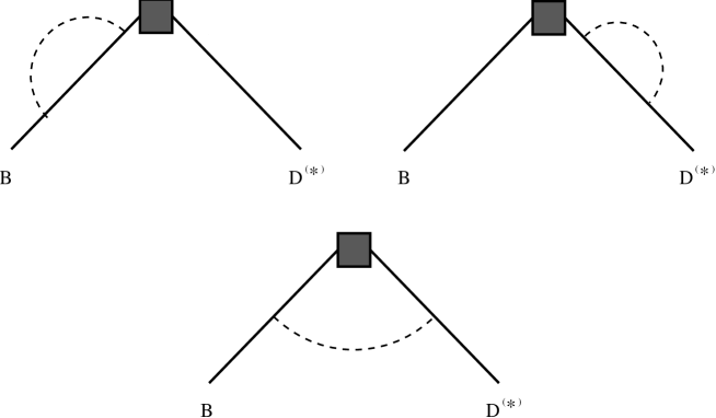
Figure 1: Diagrams for the calculation of one-loop chiral corrections to the $B\to D^{(*)}$ transition matrix element. The box represents the $b\to c$ weak current, the dashed line a light pseudoscalar.

The dominant corrections at zero recoil, i.e. $v=v^{\prime}$, are of special interest and have been computed in [91, 92]. According to Luke’s theorem, these corrections appear at the order $1/m_{Q}^{2}$. This class of corrections should not be confused with those coming from the $1/m_{Q}^{2}$ terms present in the effective lagrangian or in the current: the $1/m_{Q}$ terms in the lagrangian, in particular the one responsible for the hyperfine mass splitting $P^{*}-P$ and the one giving the splitting between the couplings $g_{D}$ and $g_{B}$, generate at one-loop $1/m_{Q}^{2}$ non-analytic corrections. The effect of the $g_{B}$ and $g_{D}$ splitting has been neglected in [91, 92]. For instance, the $B\to D^{(*)}$ matrix element at the recoil point $v=v^{\prime}$, as computed by the formulas of appendix A, is [92]

$$<D(v)|J^{\bar{c}b}_{\mu}|B(v)> = 2v_{\mu}\left[1+C(\mu)/m_{c}^{2}+\right.$$

$$- \left.{3g^{2}\over 2}\left({\Delta_{c}\over 4\pi f}\right)^{2}\left[f(\Delta_{c}/m_{\pi})+\log(\mu^{2}/m_{\pi}^{2})\right]\right]$$

$$<D^{*}(v,\epsilon)|J^{\bar{c}b}_{\mu}|B(v)> = 2\epsilon^{*}_{\mu}\left[1+C^{\prime}(\mu)/m_{c}^{2}+\right.$$ (168)

$$- \left.{g^{2}\over 2}\left({\Delta_{c}\over 4\pi f}\right)^{2}\left[f(-\Delta_{c}/m_{\pi})+\log(\mu^{2}/m_{\pi}^{2})\right]\right]$$

where $C$ and $C^{\prime}$ stand for tree level counter-terms and

$$f(x)=\int_{0}^{\infty}dz{z^{4}\over(z^{2}+1)^{3/2}}\left(\frac{1}{[(z^{2}+1)^{1/2}+x]^{2}}-\frac{1}{z^{2}+1}\right)~{}~{}.$$ (169)

In (168) only the dependence on $\Delta_{c}=M_{D^{*}}-M_{D}$ has been kept, discarding the $\Delta_{b}$ terms and those proportional to the $g_{B}-g_{D}$ splitting. Numerically, for $\mu=1\;GeV$ and $g=0.38$, the correction from the logarithmically enhanced term in (168) is $-0.6\%$, and the correction from $f(x)$ is $0.3\%$.

A complete calculation of the $1/m_{Q}$ and $SU(3)$ breaking corrections to the $B_{a}\to D^{(*)}_{a}l\nu_{l}$ process has been performed in [93]. This analysis includes non-analytic terms arising from chiral loops and the analytic counterterms, but it lacks predictive power due to the introduction of many unknown effective parameters.

In the $SU(3)$ limit, the Isgur-Wise function is independent of light quark flavor of the initial and final mesons, i.e.

$$\xi_{u}=\xi_{d}=\xi_{s}~{}~{},$$ (170)

where $\xi_{u,d,s}$ is the Isgur-Wise function occurring respectively in $B_{u,d,s}$ decays. In [94, 91] the leading corrections to the equality (170) have been computed in chiral perturbation theory, giving [91]

$$\frac{{\xi_{s}(v\cdot v^{\prime})}}{{\xi_{u,d}(v\cdot v^{\prime})}} = 1+\frac{g^{2}\Omega(v\cdot v^{\prime})}{16\pi^{2}f_{\pi}^{2}}\left[m_{K}^{2}\log\left(m_{K}^{2}/\mu^{2}\right)\right.$$ (171)

$$+ \left.\frac{1}{2}m_{\eta}^{2}\log\left(m_{\eta}^{2}/\mu^{2}\right)-\frac{3}{2}m_{\pi}^{2}\log\left(m_{\pi}^{2}/\mu^{2}\right)\right]$$

where

$$\Omega(x) = -1+\frac{2+x}{2\,\sqrt{x^{2}-1}}\;\;\log\left(\frac{x+1+\sqrt{x^{2}-1}}{x+1-\sqrt{x^{2}-1}}\right)$$ (172)

$$+ \frac{x}{4\,\sqrt{x^{2}-1}}\;\;\log\left(\frac{x-\sqrt{x^{2}-1}}{x+\sqrt{x^{2}-1}}\right)~{}~{}.$$

In (171) the analytic counterterms are neglected. Numerically, the nonanalytic chiral correction is a few percent.

We mention here another calculation in the framework of the heavy meson chiral perturbation theory, the ratio of the parameters $B_{B_{s}}$ and $B_{B}$, entering in the analysis of $B_{(s)}-{\bar{B}_{(s)}}$ mixing and defined as:

$$<\bar{B}(v)|\bar{b}\gamma_{\mu}(1-\gamma_{5})d\ \bar{b}\gamma^{\mu}(1-\gamma_{5})d|B(v)> = {8\over 3}f_{B}^{2}B_{B}$$ (173)

$$<\bar{B}_{s}(v)|\bar{b}\gamma_{\mu}(1-\gamma_{5})s\ \bar{b}\gamma^{\mu}(1-\gamma_{5})s|B_{s}(v)> = {8\over 3}f_{B_{s}}^{2}B_{B_{s}}$$ (174)

In the chiral symmetry limit $B_{B_{s}}/B_{B}=1$. For non-zero strange quark mass, the ratio is no longer equal to $1$, and the one loop chiral corrections, arising from the diagrams of figure 2, are [95]:

$${B_{B_{s}}\over B_{B}} = 1-{2\over 5}\frac{\left(1-3g^{2}\right)}{16\pi^{2}f_{\pi}^{2}}\left[m_{K}^{2}\log\left(m_{K}^{2}/\mu^{2}\right)+\right.$$ (175)

$$+ \left.\frac{1}{2}m_{\eta}^{2}\log\left(m_{\eta}^{2}/\mu^{2}\right)-\frac{3}{2}m_{\pi}^{2}\log\left(m_{\pi}^{2}/\mu^{2}\right)\right]$$

Using $\mu=1\;GeV$ and $g\simeq 0.38$ the previous formula gives $B_{B_{s}}/B_{B}\simeq 1.03$.

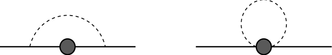
Figure 2: Diagrams appearing in the calculation of one-loop chiral corrections to the $B-{\bar{B}}$ mixing. The self-energy diagrams are not shown. The dot represents the $\Delta B=2$ operator

4.2 The $B\to D^{(*)}\pi l\nu_{l}$ decay

Another application of the chiral lagrangian can be found in the semileptonic decays of $B$ into a charmed meson with the emission of a single soft pion, i.e. $B\to D^{(*)}\pi l\nu_{l}$. The phenomenological heavy-to-heavy leading current [6]:

$$J_{\mu}^{cb}=-\xi(v\cdot v^{\prime})<{\bar{H}}^{(c)}_{a}\gamma_{\mu}(1-\gamma_{5})H^{(b)}_{a}>$$ (176)

does not depend on the pion field, and therefore the amplitude with emission of a single pion is dominated by pole diagrams, where the pion is emitted by the initial $B$ or the final $D^{(*)}$, and is proportional to the coupling $g$. The two diagrams are shown in figure 3.

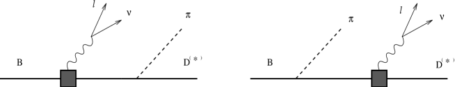
Figure 3: Pole diagrams for the $B\to D^{(*)}\pi l\nu_{l}$ decay. The square represents the $b\to c$ current, the dashed line is the pion

These decays might be used to determine the value of $g$, or even to test the heavy quark flavour symmetry prediction for the $D^{*}D\pi$ and $B^{*}B\pi$ vertices $g_{B}=g_{D}=g$. Moreover these processes may give indications on resonance effects.

The chiral calculation is reliable only in the kinematical region of soft pions. In the decay $B\to D\pi l\nu_{l}$, the soft pion domain is a large fraction due to the inclusion of the cascade decay $B\to D^{*}l\nu_{l}\to D\pi l\nu_{l}$. This process has been treated by various authors [96, 97, 98], and the analysis has been extended to $B\to D^{*}\pi l\nu_{l}$ in [99, 97, 100]: in [100], in addition to the ground state mesons $D,D^{*},B$ and $B^{*}$, also the contribution of the low-lying positive parity $0^{+}$ and $1^{+}$ resonances and some radially excited states is estimated.

4.3 The heavy-to-light effective current

The weak current for the transition from a heavy to a light quark, $Q\to q_{a}$, is given at the quark level by ${\bar{q}}_{a}\gamma_{\mu}(1-\gamma_{5})Q$; when written in terms of a heavy meson and light pseudoscalars [10], it assumes the form, at the lowest order in the light meson derivatives,

$$L^{\mu}_{a}=\frac{i{\hat{F}}}{2}<\gamma^{\mu}(1-\gamma_{5})H_{b}\xi^{\dagger}_{ba}>~{}~{}.$$ (177)

This operator transforms as $({\bar{3}}_{L},1_{R})$ under $SU(3)_{L}\times SU(3)_{R}$, i.e. analogously to the quark weak current, and is uniquely defined at this order in the chiral expansion.

From the definition of decay constant of a heavy meson $P$

$$<0|{\bar{q}}_{a}\gamma^{\mu}\gamma_{5}Q|P_{b}(p)>=ip^{\mu}f_{P_{a}}\delta_{ab}$$ (178)

one gets

$$f_{P_{a}}=\frac{{\hat{F}}}{\sqrt{M_{P}}}~{}~{}.$$ (179)

We note that in the infinite quark mass limit, $M_{P_{a}}\to m_{Q}$, and there is no dependence on the light flavour. The previous formula shows the $1/\sqrt{m_{Q}}$ scaling of the heavy meson leptonic decay constant in the $m_{Q}\to\infty$ limit, and its light-flavour independence in the chiral limit (we neglect the small logarithmic dependence of $\hat{F}$ on $m_{Q}$). In section 3.1.2 we have already discussed the various determinations of ${\hat{F}}$, see eqs. (95), (96).

Higher derivative, spin breaking, and $SU(3)$ breaking current operators are written explicitly in [35]: their introduction adds many unknown effective parameters, and they correct the leading behaviour (179). Lattice calculation [101] and QCD sum rules [62, 73] indicate that the $1/m_{Q}$ corrections are sizeable at least for $f_{D}$.

The current describing weak interactions between pseudoscalar Goldstone bosons and the positive parity $S$ fields is introduced in a similar way:

$$\hat{L}^{\mu}_{a}=\frac{i\hat{F}^{+}}{2}<\gamma^{\mu}(1-\gamma_{5})S_{b}\xi^{\dagger}_{ba}>$$ (180)

The analysis done in [79], based on QCD sum rules, gives for ${\hat{F}}^{+}$:

$${\hat{F}}^{+}\simeq 0.46\;GeV^{3/2}~{}~{}.$$ (181)

The current describing the interaction of the $H$ fields with the light vector mesons, is, at the lowest order in the derivatives:

$$L_{1a}^{\mu} = \alpha_{1}<\gamma^{\rho}(1-\gamma_{5})H_{b}v_{\rho}(\rho^{\mu}-V^{\mu})_{bc}\xi^{\dagger}_{ca}>+$$ (182)

$$+ \alpha_{2}<\gamma^{\mu}(1-\gamma_{5})H_{b}v_{\rho}(\rho^{\rho}-V^{\rho})_{bc}\xi^{\dagger}_{ca}>+$$

$$+ \alpha_{3}<\gamma^{\rho}(1-\gamma_{5})H_{b}v^{\mu}(\rho_{\rho}-V_{\rho})_{bc}\xi^{\dagger}_{ca}>~{}~{}.$$

The current (182) is of the next order as compared to the currents (177) and (180), and does not contribute to the leptonic decay constant $f_{P}$. As we shall see below, the term in (182) proportional to $\alpha_{1}$ contributes in a leading way to the $A_{1}$ form factor in the $P\to\rho$ semileptonic matrix element, while the terms proportional to $\alpha_{2}$ and $\alpha_{3}$ contribute to the $A_{2}$ form factors, but they are subleading with respect to the pole diagram contribution.

We observe that there is no similar coupling between the fields $T^{\mu}$, defined in (24) and $\xi$. Indeed (177) and (180) also describe the matrix element between the meson and the vacuum, and this coupling vanishes for the $1^{+}$ and $2^{+}$ states having $s_{l}=3/2$. This can be proved explicitly by considering the current matrix element ($A^{\mu}=\overline{q}_{a}\gamma^{\mu}\gamma_{5}Q$):

$$<0|A^{\mu}|\tilde{D}_{1}>=\tilde{f}\epsilon^{\mu}~{}~{},$$ (183)

where $\tilde{D}_{1}$ is the $1^{+}$ partner in the $s_{l}=3/2$ multiplet. Using the heavy quark spin symmetry, (183) turns out to be proportional to the matrix element of the vector current between the vacuum and the $2^{+}$ state, which vanishes.

4.4 Chiral corrections for $f_{P_{s}}/f_{P}$

In the chiral limit, the leptonic decay constant does not depend on the light flavour, i.e.

$$\frac{f_{P_{s}}}{f_{P}}=1~{}~{}.$$ (184)

As discussed in section (3.2), one can obtain an estimate of the $SU(3)$ violations by computing the non-analytic terms arising from the chiral loops.

The one-loop diagrams contributions to the leptonic decay constant $f_{P}$ are shown in fig. 4, and have been computed in [95, 91], keeping only the “log-enhanced” terms of the form $m^{2}\log(m^{2}/\mu^{2})$. For the ratio $f_{D_{s}}/f_{D}$ one has:

$$\frac{f_{D_{s}}}{f_{D}}=1-\frac{1}{32\pi^{2}f_{\pi}^{2}}\left[m_{K}^{2}\log(\frac{m_{K}^{2}}{\mu^{2}})+\frac{1}{2}m_{\eta}^{2}\log(\frac{m_{\eta}^{2}}{\mu^{2}})-\frac{3}{2}m_{\pi}^{2}\log(\frac{m_{\pi}^{2}}{\mu^{2}})\right](1+3g^{2})~{}~{}.$$ (185)

The corrections proportional to $g^{2}$ arise from the self-energy diagrams, fig. 4b, while the diagram 4c gives the $g$-independent corrections. The diagram 4d, linear in $g$, vanishes at the leading order in $1/m_{Q}$. Using $g\simeq 0.38$ in (185), one gets $f_{D_{s}}/f_{D}\simeq 1.11$.

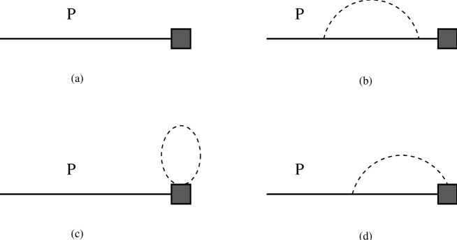
Figure 4: Diagrams for the calculation of one-loop chiral corrections to the heavy meson leptonic decay constant $f_{P}$. The box represents the $b\to q$ weak current, the dashed line a light pseudoscalar.

The excited positive parity heavy mesons contribute to $SU(3)$ violating effects as virtual intermediate states in chiral loops. In Ref.[102] the “log-enhanced” terms due to these excited-state loops have been computed: some of them are proportional to $h^{2}$ and others depend linearly on $h$, $h$ being the coupling of the vertex $P^{**}P\pi$. In [102] it has been pointed out that these terms could be numerically relevant and could invalidate the chiral estimate based only on the states $D$ and $D^{*}$; as discussed in section 3.4 the coupling $h$ is estimated by QCD sum rules in [80], with the result $h\simeq-0.5$, see eqs. (150, 154), where a more accurate chiral computation of the ratio $f_{D_{s}}/f_{D}$ is performed. We present here some details of the calculation: the vertices and the integrals needed for the loop integration can be found respectively in appendices A and B.

The self-energy diagrams 4b give the following wave function renormalization factors:

$$Z_{D} = 1-\frac{3g^{2}}{16\pi^{2}f_{\pi}^{2}}\left[3/2C_{1}(\Delta_{D^{*}D},\Delta_{D^{*}D},m_{\pi})+C_{1}(\Delta_{D^{*}_{s}D},\Delta_{D^{*}_{s}D},m_{K})+\frac{1}{6}C_{1}(\Delta_{D^{*}D},\Delta_{D^{*}D},m_{\eta})\right]$$ (186)

$$+ \frac{h^{2}}{16\pi^{2}f_{\pi}^{2}}\left[3/2C(\Delta_{P_{0}P},\Delta_{P_{0}P},m_{\pi})+C(\Delta_{P_{0s}P},\Delta_{P_{0s}P},m_{K})+\right.$$

$$+ \left.\frac{1}{6}C(\Delta_{P_{0}P},\Delta_{P_{0}P},m_{\eta})\right]$$

$$Z_{D_{s}} = 1-\frac{3g^{2}}{16\pi^{2}f_{\pi}^{2}}\left[2C_{1}(\Delta_{D^{*}D_{s}},\Delta_{D^{*}D_{s}},m_{K})+\frac{2}{3}C_{1}(\Delta_{D^{*}D},\Delta_{D^{*}D},m_{\eta})\right]$$ (187)

$$+ \frac{h^{2}}{16\pi^{2}f_{\pi}^{2}}\left[2C(\Delta_{P_{0}P_{s}},\Delta_{P_{0}P_{s}},m_{K})+\frac{2}{3}C(\Delta_{P_{0}P},\Delta_{P_{0}P},m_{\eta})\right]$$

where the mass splittings $\Delta_{P^{*}P}=M_{P^{*}}-M_{P}$, $\Delta_{P^{*}P_{s}}=M_{P^{*}}-M_{P_{s}}$, and $\Delta_{P_{s}^{*}P}=M_{P_{s}^{*}}-M_{P}$ are ${\cal O}(1/m_{Q})$, while the mass splittings $\Delta_{P_{0}P}=M_{P_{0}}-M_{P}$, $\Delta_{P_{0s}P}=M_{P_{0s}}-M_{P}$, and $\Delta_{P_{0}P_{s}}=M_{P_{0}}-M_{P_{s}}$ between excited and ground states are finite in the limit $m_{Q}\to\infty$.

The functions $C_{1}$ and $C$ come from the loop integration and are defined in appendix B (here we use $\hat{\Delta}=0$).

The diagram 4c gives the same contribution as in (185), while the diagram 4d is linear in $h$ (the analogous term proportional to $g$ vanishes), and proportional to ${\hat{F}}^{+}$: combining all the diagrams one obtains [80]:

$$f_{D} = \frac{{\hat{F}}}{\sqrt{M_{D}}}\left[1-\frac{1}{32\pi^{2}f_{\pi}^{2}}\left[\frac{3}{2}m_{\pi}^{2}\log(\frac{m_{\pi}^{2}}{\mu^{2}})+m_{K}^{2}\log(\frac{m_{K}^{2}}{\mu^{2}})+\frac{1}{6}m_{\eta}^{2}\log(\frac{m_{\eta}^{2}}{\mu^{2}})\right]\right.$$ (188)

$$- \frac{3g^{2}}{32\pi^{2}f_{\pi}^{2}}\left[\frac{3}{2}C_{1}(\Delta_{D^{*}D},\Delta_{D^{*}D},m_{\pi})+C_{1}(\Delta_{D^{*}_{s}D},\Delta_{D^{*}_{s}D},m_{K})+\frac{1}{6}C_{1}(\Delta_{D^{*}D},\Delta_{D^{*}D},m_{\eta})\right]$$

$$+ \frac{h^{2}}{32\pi^{2}f_{\pi}^{2}}\left[\frac{3}{2}C(\Delta_{P_{0}P},\Delta_{P_{0}P},m_{\pi})+C(\Delta_{P_{0s}P},\Delta_{P_{0s}P},m_{K})+\frac{1}{6}C(\Delta_{P_{0}P},\Delta_{P_{0}P},m_{\eta})\right]$$

$$+ \left.\frac{{\hat{F}}^{+}}{{\hat{F}}}\frac{h}{16\pi^{2}f_{\pi}^{2}}\left[\frac{3}{2}C(\Delta_{P_{0}P},0,m_{\pi})+C(\Delta_{P_{0s}P},0,m_{K})+\frac{1}{6}C(\Delta_{P_{0}P},0,m_{\eta})\right]\right]$$

$$f_{D_{s}} = \frac{{\hat{F}}}{\sqrt{M_{D}}}\left[1-\frac{1}{32\pi^{2}f_{\pi}^{2}}\left[2m_{K}^{2}\log(\frac{m_{K}^{2}}{\mu^{2}})+\frac{2}{3}m_{\eta}^{2}\log(\frac{m_{\eta}^{2}}{\mu^{2}})\right]\right.$$ (189)

$$- \frac{3g^{2}}{32\pi^{2}f_{\pi}^{2}}\left[2C_{1}(\Delta_{D^{*}D_{s}},\Delta_{D^{*}D_{s}},m_{K})+\frac{2}{3}C_{1}(\Delta_{D^{*}D},\Delta_{D^{*}D},m_{\eta})\right]$$

$$+ \frac{h^{2}}{32\pi^{2}f_{\pi}^{2}}\left[2C(\Delta_{P_{0}P_{s}},\Delta_{P_{0}P_{s}},m_{K})+\frac{2}{3}C(\Delta_{P_{0}P},\Delta_{P_{0}P},m_{\eta})\right]$$

$$+ \left.\frac{{\hat{F}}^{+}}{{\hat{F}}}\frac{h}{16\pi^{2}f_{\pi}^{2}}\left[2C(\Delta_{P_{0}P_{s}},0,m_{K})+\frac{2}{3}C(\Delta_{P_{0}P},0,m_{\eta})\right]\right]\;.$$

From the previous formulas, using $\Delta_{P_{0}P}=0.5\;GeV$, $\mu=1$, ${\hat{F}}^{+}=0.46\;GeV^{3/2}$ and ${\hat{F}}=0.30\;GeV^{3/2}$, one gets numerically:

$$f_{D} = \frac{{\hat{F}}}{\sqrt{M_{D}}}\left(1+0.09+0.003g^{2}-0.33h^{2}-1.00h\right)$$ (190)

$$f_{D_{s}} = \frac{{\hat{F}}}{\sqrt{M_{D}}}\left(1+0.17+0.59g^{2}-0.66h^{2}-1.15h\right)\;.$$ (191)

In the previous formulas we have kept only the leading order in the $1/m_{Q}$, i.e. we have put $\Delta_{D^{*}D}=0$ in (188) and (189).

It is found that the terms ${\cal O}(h^{2})$ and ${\cal O}(h)$, while important, tend to cancel out in (190, 191) and that the ratio of leptonic decay constants is numerically the same as obtained from (185):

$$\frac{f_{D_{s}}}{f_{D}}\simeq 1.10~{}~{}.$$ (192)

These values are obtained by using $g=0.38$ and $h=-0.5$.

The formula (185) is valid at the leading order in $1/m_{Q}$, and in this limit it is the same for $B$ and $D$ systems. In other terms, the double ratio $R_{1}$

$$R_{1}=\frac{f_{B_{s}}/f_{B}}{f_{D_{s}}/f_{D}}$$ (193)

is equal to $1$ in the chiral limit and in the heavy quark limit, separately. To see how $R_{1}$ deviates from unity one has to take into account the $1/M$ terms in the chiral effective lagrangian and in the effective current. As discussed in [35], four new parameters contribute at the order $1/m_{Q}$ to the leptonic decay constants: two of them, $\rho_{1}$ and $\rho_{2}$, come from the $1/m_{Q}$ terms in the current as

$$L^{\mu}_{a} = \frac{i{\hat{F}}}{2}(1+\frac{\rho_{1}}{M_{P}})<\gamma^{\mu}(1-\gamma_{5})H_{b}\xi^{\dagger}_{ba}>+$$ (194)

$$+ \frac{i{\hat{F}}}{2}\frac{\rho_{2}}{M_{P}}<\gamma_{\alpha}\gamma^{\mu}(1-\gamma_{5})\gamma^{\alpha}H_{b}\xi^{\dagger}_{ba}>$$

and they modify the leptonic decay constants as follows

$$\sqrt{M_{P}}f_{P} = {\hat{F}}\left(1+\frac{\rho_{1}+2\rho_{2}}{M_{P}}\right)$$

$$\sqrt{M_{P}}f_{P^{*}} = {\hat{F}}\left(1+\frac{\rho_{1}-2\rho_{2}}{M_{P}}\right)~{}~{}.$$ (195)

The two parameters $\rho_{1}$ and $\rho_{2}$ can be related to the HQET matrix elements $G_{K}$ and $G_{\Sigma}$ defined in eq. (123), and estimated by QCD sum rules in [62, 73].

The other two couplings, $g_{1}$ and $g_{2}$, have been already introduced in (46), and they parameterize the $1/M$ corrections to the couplings $g_{P^{*}P\pi}$ and $g_{P^{*}P^{*}\pi}$:

$$g_{P^{*}P^{*}\pi} = g+\frac{1}{M_{P}}(g_{1}+g_{2})$$ (196)

$$g_{P^{*}P\pi} = g+\frac{1}{M_{P}}(g_{1}-g_{2})~{}~{}.$$ (197)

For the chiral correction to the double ratio $R_{1}$, neglecting as usual the analytic counterterms, only the quantity $g_{1}-g_{2}$, i.e. the $1/M_{P}$ correction to $g_{P^{*}P\pi}$, is relevant, and one gets [35]

$$R_{1}-1=-0.11g^{2}-0.06\;g(g_{1}-g_{2})~{}GeV^{-1}~{}~{}.$$ (198)

5 Heavy-to-light semileptonic exclusive decays

Most of the known CKM matrix elements have been determined using semileptonic decays. In particular, from semileptonic $B$ decays one can extract $V_{cb}$ and $V_{ub}$.

The extraction of the value of $V_{cb}$ from the exclusive process $B\to D^{*}l\nu_{l}$ has been studied in the HQET context, and we mentioned it before. The situation for $V_{ub}$ is apparently more uncertain, both for the inclusive and the exclusive semileptonic rates. Its determination is one of the most important goals in $B$ physics, but it involves great experimental and theoretical difficulties. At the moment there is a safe experimental evidence for $b\to u$ transitions, and experimental data on the $B\to\pi l\nu_{l}$ and $B\to\rho l\nu_{l}$ exclusive processes have been presented by the CLEO II collaboration [103].

The interpretation of the inclusive $b\to u$ semileptonic rate is difficult because of the dominant $b\to c$ background: to eliminate it, one works beyond the end-point region of the lepton momentum spectrum for $b\to c$ processes. This is a very small fraction of the phase space, where theoretical inclusive models have relevant uncertainties.

Predictions for the exclusive channels $B\to X_{u}l\nu_{l}$ are also model dependent, and here HQET is much less useful than in the $B\to D$ process, because of the presence of a light meson in the final state. We shall show in the following sections how to relate $B\to\pi l\nu_{l}$ to $D\to\pi l\nu_{l}$, and $B\to\rho l\nu_{l}$ to $D\to\rho l\nu_{l}$, in the $b$ and $c$ infinite mass limit. The main problem of this approach are the $1/m_{c}$ corrections, potentially relevant and not under control.

The effective lagrangian approach can shed light on these semileptonic decays and can give indications on the values of the relevant form factors at the zero recoil point. In order to extract information from the experimental data the complete $q^{2}$ dependence of the form factors is required, which goes beyond the chiral lagrangian approach. For this reason external inputs, either phenomenological or purely theoretical, are required, and, in the next section, we shall discuss this issue in some details.

5.1 Form factors

We introduce now form factors that parameterize the hadronic matrix elements of the weak currents.

In the case of semileptonic decays, $P\to P^{\prime}l\nu_{l}$ ($P$, $P^{\prime}$ pseudoscalar mesons) there is no contribution from the axial-vector part of the current and the matrix element can be written as

$$<P^{\prime}(p^{\prime})|V^{\mu}|P(p)>=\big{[}(p+p^{\prime})^{\mu}+\frac{M_{P^{\prime}}^{2}-M_{P}^{2}}{q^{2}}q^{\mu}\big{]}F_{1}(q^{2})-\frac{M_{P^{\prime}}^{2}-M_{P}^{2}}{q^{2}}q^{\mu}F_{0}(q^{2})$$ (199)

where $V_{\mu}={\bar{q}}^{\prime}\gamma_{\mu}Q$ and $q=p-p^{\prime}$. There is no singular behaviour at $q^{2}=0$ because $F_{1}(0)=F_{0}(0)$.

The form factor $F_{1}(q^{2})$ can be associated, in a dispersion relation approach, to intermediate states with quantum numbers $J^{P}=1^{-}$, and $F_{0}(q^{2})$ to states with $J^{P}=0^{+}$. In the limit of massless lepton, the terms proportional to $q_{\mu}$ in (199) do not contribute to the rate, so that only the form factor $F_{1}(q^{2})$ is relevant.

For the pseudoscalar to vector matrix elements also the axial-vector current contributes and four form factors are required:

$$<V(\epsilon,p^{\prime})| ( V^{\mu}-A^{\mu})|P(p)>=\frac{2V(q^{2})}{M_{P}+M_{V}}\epsilon^{\mu\nu\alpha\beta}\epsilon^{*}_{\nu}p_{\alpha}p^{\prime}_{\beta}$$ (200)

$$+ i(M_{P}+M_{V})\left[\epsilon^{*\mu}-\frac{\epsilon^{*}\cdot q}{q^{2}}q^{\mu}\right]A_{1}(q^{2})$$

$$- i\frac{\epsilon^{*}\cdot q}{(M_{P}+M_{V})}\left[(p+p^{\prime})^{\mu}-\frac{M_{P}^{2}-M_{V}^{2}}{q^{2}}q^{\mu}\right]A_{2}(q^{2})$$

$$+ i\epsilon^{*}\cdot q\frac{2M_{V}}{q^{2}}q^{\mu}A_{0}(q^{2})~{}~{},$$

where

$$A_{0}(0)=\frac{M_{V}-M_{P}}{2M_{V}}A_{2}(0)+\frac{M_{V}+M_{P}}{2M_{V}}A_{1}(0)~{}~{}.$$ (201)

Neglecting the lepton mass, only the form factors $V(q^{2})$, $A_{1}(q^{2})$ and $A_{2}(q^{2})$ contribute to the decay rate. The form factors $A_{1}$ and $A_{2}$ can be associated to $J^{P}=1^{+}$ intermediate states, and $V$ to $J^{P}=1^{-}$ states.

The form factor dependence on $q^{2}$ is still an open question, and, at the present time, there is no general theoretical agreement. Quark model calculations are based on meson wave functions, generally derived by some wave equation, and make use of them to compute hadronic matrix elements. These calculations are normally reliable only at some specific value of $q^{2}$, and the dependence on the variable $q^{2}$ has to be assumed as an additional hypothesis. The physical region for semileptonic decays covers the range $0\leq q^{2}\leq q^{2}_{max}=(M_{P}-m_{\pi})^{2}$ (in the limit of massless leptons). Close to $q^{2}_{max}$, the form factors should be dominated by the nearest $t$-channel pole, located at the mass of the lightest heavy meson exchanged in that channel.

With decreasing $q^{2}$, the influence of the pole becomes weaker: in a dispersion relation the form factor can be written as a $P^{*}$ pole contribution ($P^{*}$ nearest pole for that channel) plus a continuum contribution, that, in the narrow width approximation, reduces to a sum over higher resonances $P_{n}$. We can therefore write, e.g., for the form factor $F_{1}$:

$$F_{1}(q^{2})=\frac{f_{P^{*}}g_{PP^{*}\pi}}{q^{2}-M^{2}_{P^{*}}}+\sum_{n}\frac{f_{P_{n}}g_{PP_{n}\pi}}{q^{2}-M^{2}_{P_{n}}}~{}~{},$$ (202)

where $g_{PP^{*}\pi}$ is the trilinear coupling among $P$, $P^{*}$ and $\pi$. In the combined limit $m_{\pi}\to 0$, $M_{P}\to\infty$, the $P^{*}$ pole contribution goes like $M_{P}^{1/2}$ when $q^{2}\to M^{2}_{P}$ ($g_{PP^{*}\pi}\sim M_{P}$), while the higher resonances contributions go only like $M_{P}^{-1/2}$, as they do not become degenerate with the $P$ in the heavy mass limit. But far away from the kinematical end point $q^{2}_{max}$, many resonances can in general contribute to the form factors. This observation leads to two-component models for the form factors [12]. In [104] it is shown that the form factors for $B\to\pi$ semileptonic decay are dominated by the $B^{*}$ pole at all $q^{2}$ in two-dimensional planar QCD; it remains to be seen if such dominance hold also in four dimensions.

The nearest pole-dominance on the whole $q^{2}$ range, i.e.

$$F(q^{2})=\frac{F(0)}{1-q^{2}/M^{2}_{pole}}$$ (203)

should therefore be taken as an additional assumption in building models, as done for instance in the popular BSW model [105]. Other dependences can be found in the literature; for example in the ISGW model [106], which is expected to work well close to $q^{2}_{\rm max}$, the extrapolation to lower $q^{2}$ is done by an exponential dependence for the form factors. It is important to stress that in general predictions for the widths are not sensitive to the assumed dependence only when the available range in $q^{2}$ is not large, as in $D$ decays: for $B$ decays into light mesons, as $B\to\pi(\rho)l\nu_{l}$, different form factor behaviours can lead to different predictions.

Experimentally, only the decay $D^{0}\to K^{-}e^{+}\nu_{e}$ allows at the moment a study of the $q^{2}$ dependence of the form factor $F_{1}$. The data are compatible with the pole form (203), but the precision is still poor. The value of the pole mass, as fitted by the data, is compatible with the $D^{*}_{s}$ mass, and the intercept $F_{1}(0)$ is [45]

$$F_{1}^{DK}(0)=0.75\pm 0.03~{}~{}.$$ (204)

The Cabibbo-suppressed decay $D\to\pi l\nu_{l}$ suffers from poor statistics: MARK III and CLEO II data, extracted with the pole-dominance hypothesis, give[45]:

$$\frac{F_{1}^{D\pi}(0)}{F_{1}^{DK}(0)} = 1.0^{+0.3}_{-0.2}\pm 0.04\;\;{\rm MARK~{}III}$$ (205)

$$= 1.3\pm 0.2\pm 0.1\;\;{\rm CLEO~{}II}~{}~{}.$$

Theoretically, QCD sum rules allow to compute the $q^{2}$ dependence of the form factors, except when close to $q^{2}_{max}$. The analyses performed in [107, 108, 109, 110, 111, 112] are generally compatible with nearest pole dominance for the vector current form factor, $F_{1}$ and $V$: for the axial form factors, $A_{1}$ and $A_{2}$, there are discrepancies among the different calculations. In [113, 108], the form factor $A_{1}^{B\to\rho}$ has an unexpected behaviour, decreasing from $q^{2}=0$ to $q^{2}=15\;GeV^{2}$: for $A_{2}^{B\to\rho}$, a moderate increase in $q^{2}$ is found, at least up to $q^{2}\simeq 15\;GeV^{2}$. For higher values of $q^{2}$ the estimate is unreliable. Such a behaviour is the result of cancellations among large terms, and therefore can suffer from relevant uncertainties. Also, in [112] the form factor $A_{1}$ decreases with $q^{2}$, while $A_{2}$ can be fitted by a pole formula. Light-cone sum rules [110] show, on the contrary, an increasing $A_{1}$, with a dependence close to the pole behaviour, and a steeper increase for $V$.

Current lattice QCD simulations cannot study directly the $b$ quark, because its mass is above the UV cut-off. Quantities are computed around the charm scale, and then extrapolated up to the $b$ mass using the Isgur-Wise scaling relations [51]. With this strategy, suggested in [114], one is forced to make assumptions on the $q^{2}$-dependence at the $b$ scale, because the extrapolation pushes the $q^{2}$ value towards $q^{2}_{max}$. For $D$ meson form factors, the determination of $q^{2}$ dependence is still poor, but compatible with pole dominance [115, 116]. Preliminary lattice computations of the $q^{2}$ dependence of the form factors $F_{1}$ and $F_{0}$ in $B\to\pi l\nu_{l}$ [117], and $A_{1}$ in $B\to\rho l\nu_{l}$ [118], seem to favor a dipole/pole fit for $F_{1}$ and $F_{0}$ respectively, and a pole behaviour for $A_{1}$: the data have however large uncertainties, and will be improved by working with heavier quark masses and by using larger lattices.

An additional constraint to the form factor $q^{2}$ dependence is provided by nonleptonic heavy meson decays. It has been shown that the commonly used form factors, when used together with the additional hypothesis of factorization to evaluate non-leptonic decay amplitudes, do not agree with the data on $B\to J/\psi K(K^{*})$ transitions [119, 120]. These non-leptonic decays can be computed, using the factorization approximation, as functions of the leptonic decay constant $f_{J/\psi}$ and the form factors $F_{1}^{BK}$, $A_{1}^{BK^{*}}$, $A_{2}^{BK^{*}}$, and $V^{BK^{*}}$, at $q^{2}=M^{2}_{J/\psi}$. The problem is to fit simultaneously the rather small ratio of vector to pseudoscalar decay rates, $\Gamma(B\to K^{*}J/\psi)/\Gamma(B\to KJ/\psi)$, and the large fraction of longitudinal polarization in $B\to J/\psi K^{*}$.

In [121], it has been shown that the discrepancy can be eliminated allowing for a non-polar behaviour of some form factors. Using the Isgur-Wise scaling laws, these authors compute the relevant form factors from the experimental data on the semileptonic transitions $D\to K(K^{*})$ at $q^{2}=0$. Subsequently they adopt for the form factors a generic dependence $(1-q^{2}/\Lambda^{2})^{-n}$, with $n=-1,0,1,2$. Simple-pole dominance corresponds to $n=1$. Three scenarios survive to the phenomenological analysis: the form factors $F_{1}$, $A_{1}$, $A_{2}$ and $V$ can only have a dependence $[n_{F},n_{1},n_{2},n_{V}]=[+1,-1,n_{2},+2]$ respectively, and $n_{2}$ can be equal to $2,1,0$ (with a preference for $n_{2}=2$). Notice that $A_{1}(q^{2})$ is linearly decreasing in these scenarios: a similar behaviour is found also in a theoretical analysis [108], at least for $q^{2}<15\;GeV^{2}$.

The hypothesis that $A_{1}$ is linearly decreasing on the whole range in $q^{2}$ is certainly not valid: the form factor should have a pole at $q^{2}=M^{2}_{1^{+}}$, which should affect the $q^{2}$ dependence at least close to the zero-recoil point. In [120] it is argued that $A_{1}$ should have a flatter $q^{2}$ dependence than the one predicted by the pole dominance.

In section 5.3 we shall present a phenomenological analysis of the $B\to V$ ($V$ light vector meson) processes, showing that a constant $A_{1}$ behaviour leads to discrepancies with the available data, when scaling laws are used to scale the form factors from $D$ to $B$ systems: the situation would be even worse for a decreasing $A_{1}$. There is thus some rough suggestions for an increasing $A_{1}$ with $q^{2}$, and in section 5.3.2 a two-component model for $A_{1}$, a constant term plus a pole term, is used with satisfactory phenomenological agreement.

In any event, further theoretical and experimental studies are needed to clarify the problem of $q^{2}$ dependence in the form factors.

5.2 $B\to\pi$ semileptonic decays

In this section we shall analyze the semileptonic exclusive decays of a heavy meson $P=B,\;D$ into a light particle belonging to the pseudoscalar octet, e.g. $\pi$.

The relevant hadronic matrix element is:

$$<\pi|{\bar{q}}\gamma_{\mu}Q|P>~{}~{}.$$ (206)

In absence of a knowledge of the hadronic current in terms of hadrons, various theoretical approaches to the evaluation of (206) have been developed: potential models, for instance in [105, 106], lattice QCD [114, 115, 116, 117], QCD sum rules [122], and the method based on the chiral and heavy quark symmetries, that we shall review here.

In general two attitudes are possible. In the first one, that we shall call the scaling approach, one relates the different hadronic matrix elements (206) using the spin and flavour symmetries. In this way for instance it is possible to relate the matrix elements $<\pi|j_{\mu}|B>$ and $<K|j_{\mu}|D>$, $\pi$ and $K$ belonging to the same chiral multiplet, and $B$ and $D$ being related by heavy flavour symmetry. In the second approach, one builds up an effective lagrangian incorporating chiral and heavy quark symmetries, and computes the form factors within such framework. The advantage of the second approach is the possibility to include in a rigorous way symmetry breaking corrections, at least formally. Both approaches lead to the same results at the leading order, and require some experimental or external inputs: in the scaling approach one starts with a known matrix element, while the effective lagrangian contains unknown couplings that are determined by the data. As we shall see, some of these couplings have also been estimated theoretically, and we shall review also these analyses.

5.2.1 The scaling approach

We shall discuss first the so-called Isgur-Wise scaling laws for the form factors. Let us parameterize the hadronic matrix element as follows:

$$<\pi(p_{\pi})|J_{\mu}|P(p_{P})>=(p_{\pi}+p_{P})_{\mu}f_{+}^{P\pi}(q^{2})+(p_{P}-p_{\pi})_{\mu}f_{-}^{P\pi}(q^{2})$$ (207)

where $q^{2}=(p_{P}-p_{\pi})^{2}$. The Isgur-Wise relations, following from the $SU(2)$ flavour symmetry between $b$ and $c$ quarks, give [51]:

$$(f_{+}+f_{-}) \sim m_{Q}^{-1/2}$$

$$(f_{+}-f_{-}) \sim m_{Q}^{+1/2}~{}~{}.$$ (208)

We have neglected here the logarithms of $m_{Q}$ arising from perturbative QCD corrections. These scaling laws are valid as long as $v\cdot p_{\pi}$ does not scale with $m_{Q}$, i.e. in the kinematical regime of soft $\pi$, close to $q^{2}_{max}=(m_{P}-m_{\pi})^{2}$. In this region $E_{\pi}\simeq m_{\pi}<<m_{Q}$. $q^{2}_{max}$ is the no recoil point, where the final scalar and the dilepton system are at rest.

Using the form factors $F_{1},F_{0}$, the eqs. (208) become, including QCD corrections,

$$F_{1}^{B\pi}(q^{2}_{max,B}) = \left[\frac{\alpha_{s}(M_{B})}{\alpha_{s}(M_{D})}\right]^{-6/25}\sqrt{\frac{M_{B}}{M_{D}}}F_{1}^{D\pi}(q^{2}_{max,D})$$ (209)

$$F_{0}^{B\pi}(q^{2}_{max,B}) = \left[\frac{\alpha_{s}(M_{B})}{\alpha_{s}(M_{D})}\right]^{-6/25}\sqrt{\frac{M_{D}}{M_{B}}}F_{0}^{D\pi}(q^{2}_{max,D}).$$ (210)

Eqs. (209) and (210) are valid in the $m_{b},\;m_{c}\to\infty$ limit. The $1/m_{c}$ corrections can be large, as we will discuss later, and can be estimated in the effective lagrangian approach.

The application of the chiral symmetry is straightforward, and, at the leading order gives:

$$F^{P\pi}(q^{2})=F^{P\pi^{\prime}}(q^{2})~{}~{}.$$ (211)

Here $\pi$ and $\pi^{\prime}$ are two arbitrary light pseudoscalar mesons, for instance $\pi$ and $K$. We notice that (211) is valid for any value of $q^{2}$.

From the knowledge of the form factors at any value of $q^{2}$ for a given decay mode one can compute a whole class of decays as follows:

• Using (211), one computes all the chiral-related decays. We notice that all the form factors related by light flavour symmetry have the same $q^{2}$-behaviour, but $F_{0}$ and $F_{1}$ can have a different behaviour.

• The Isgur-Wise scaling laws (209) and (211) allow to relate $B$ and $D$ form factors, at least close to $q^{2}_{max}$.

• The strongest assumption concerns the evolution in $q^{2}$ of the scaled form factors. The $B$ decay rates are quite sensitive to the explicit $q^{2}$ dependence, while for $D$ decays the $q^{2}$-range is much smaller.

We proceed to the computation of the form factors, widths and branching ratios for the semileptonic decays of a heavy meson into a light scalar, following the strategy we have described. Such an approach was followed in [14, 123] for the semileptonic decays, and in [119, 120] to compute the $B\to K(K^{*})$ form factors.

For the form factor $F_{1}$ we shall assume a simple pole behaviour, which, as we have already discussed, agrees with present experimental and theoretical evidence. As an input, we use the decay $D\to Kl\nu_{l}$, i.e. the form factor at $q^{2}=0$ (204). For chirally-related decays, we impose the same value to the form factors at $q^{2}=0$. For generic $q^{2}$ we have

$$F_{1}(q^{2})=\frac{F_{1}(0)}{1-q^{2}/M^{2}_{P*}}~{}~{}.$$ (212)

The $1^{-}$ pole $P^{*}$ can be a strange or a non-strange heavy meson, depending on the decay mode: their mass difference $\Delta_{s}=M_{P_{s}}-M_{P}\simeq 100\;MeV$ is a chiral breaking effect, which we will not neglect.

Let us make some comments on the Isgur-Wise scaling law, which follows from the observation that the matrix element $<\pi(p_{\pi})|J_{\mu}|P(v)>$ behaves as $\sqrt{m_{Q}}$, in the limit $v\cdot p_{\pi}<<m_{Q}\to\infty$. These asymptotic scaling laws have $1/m_{Q}$ corrections

$$<\pi(p_{\pi})|J_{\mu}|P(v)>\sim\sqrt{m_{Q}}\left(1+{\cal O}\left(\frac{\Lambda_{QCD}}{m_{Q}}\right)+{\cal O}\left(\frac{v\cdot p_{\pi}}{m_{Q}}\right)+{\cal O}\left(\frac{m_{\pi}}{m_{Q}}\right)\right)~{}~{},$$ (213)

and a number of different choices for the scaling relations are possible. They are all compatible with the asymptotic behaviour, but differ for corrections of the type indicated in (213). Eqs. (209) and (210) is a possible one, but other choices might be done. For instance we could have taken, for $F_{1}$, neglecting QCD corrections:

$$\frac{F_{1}^{B\pi}}{F_{1}^{D\pi}}\Big{|}_{(q^{2}_{max})}=\sqrt{\frac{M_{D}}{M_{B}}}\frac{M_{B}+m_{\pi}}{M_{D}+m_{\pi}}$$ (214)

which reduces to (209) in the $M_{B},M_{D}\to\infty$ limit. Notice that the “soft scaling” (214) can lead to results numerically different when the mass of the light final meson is not so small, as for instance in the case of $K$ or $K^{*}$. In these cases the differences between (209) and (214) are of the order $m_{K}/M_{D}$, or $m_{K^{*}}/M_{D}$. Other possible scaling forms can be found in [119, 120]. QCD radiative corrections, written in (209,210), are of the order of 10%: and therefore they can be neglected within our approximations.

The chiral limit, $m_{\pi}\to 0$, presents some subtleties. In order to examine them, let us find the scaling laws at $q^{2}=0$, as arising from the simple-pole behaviour (212) and the asymptotic scaling at $q^{2}_{max}$. One finds:

$$\frac{F_{1}^{B\pi}}{F_{1}^{D\pi}}\Big{|}_{q^{2}=0}\simeq\frac{M_{D}}{M_{B}}\frac{\Delta_{B}+m_{\pi}}{\Delta_{D}+m_{\pi}}\frac{F_{1}^{B\pi}}{F_{1}^{D\pi}}\Big{|}_{q^{2}_{max}}\;.$$ (215)

In the $m_{b},m_{c}\to\infty$ limit, $\Delta_{P}=M_{P^{*}}-M_{P}\to 0$, and one gets:

$$\frac{F_{1}^{B\pi}}{F_{1}^{D\pi}}\Big{|}_{q^{2}=0}\simeq\sqrt{\frac{M_{D}}{M_{B}}}~{}~{}.$$ (216)

On the other hand, performing first the $m_{\pi}\to 0$ limit in (215), one finds:

$$\frac{F_{1}^{B\pi}}{F_{1}^{D\pi}}\Big{|}_{q^{2}=0}\simeq\left(\frac{M_{D}}{M_{B}}\right)^{\frac{3}{2}}\;.$$ (217)

The contradiction between (216) and (217) means a breaking of the naive scaling laws at $q^{2}_{max}$ in the chiral limit: as shown by [51], in the limit $m_{\pi}\to 0$ (209) becomes:

$$\frac{F_{1}^{B\pi}}{F_{1}^{D\pi}}\Big{|}_{q^{2}_{max}}\simeq\left(\frac{M_{B}}{M_{D}}\right)^{\frac{3}{2}}~{}~{}.$$ (218)

This behaviour can be explained, as we shall see, from the polar diagram with exchange of the $P^{*}$. Therefore, combining (215) and (218), we find also in the chiral limit the scaling law (216), which we shall use in the subsequent analysis.

Using (204) as an input, we get:

$$F_{1}^{BK}(0)\simeq 0.45~{}~{}.$$ (219)

As previously discussed, the uncertainties due to scale corrections are expected to be of the order $m_{K}/M_{D}$, i.e. about 30 %. The uncertainties due to deviations from the polar behaviour of the form factor are hard to estimate and essentially unknown.

We could use as an input the Cabibbo-suppressed decay $D\to\pi$, which has however larger experimental errors. The scaling uncertainties, moreover, even if probably smaller than in the case of a final $K$, are expected to be of order ${\bar{\Lambda}}/M_{D}$ (${\bar{\Lambda}}=M_{P}-m_{Q}$) and not of order $m_{\pi}/M_{D}$ only; therefore they could be really significant.

The prediction for widths and branching ratios following from (219) and chiral symmetry are reported in table 3.

Table 3: Predictions for semileptonic $D$ and $B$ decays in a pseudoscalar meson, in the scaling approach. We have neglected the $\eta~{}-\eta^{\prime}$ mixing. The branching ratios and the widths for $B$ must be multiplied for $|V_{ub}/0.0032|^{2}$. We assume $\tau_{B_{s}}=\tau_{B^{0}}=\tau_{B^{+}}=1.55~{}ps.$

Decay	$F_{1}(0)$	BR	exp. BR
$D^{0}\to\pi^{-}$	0.75	$3.4\cdot 10^{-3}$	$(3.9^{+2.3}_{-1.2})\cdot 10^{-3}$ [45]
$D^{+}\to\eta$	0.31	$6.9\cdot 10^{-4}$
$D_{s}\to\eta$	0.61	$3.2\cdot 10^{-2}$
$D_{s}\to K^{0}$	0.75	$4.2\cdot 10^{-3}$
$B^{0}\to\pi^{-}$	0.45	$2.2\cdot 10^{-4}$	$(1.63\pm 0.46\pm 0.34)\cdot 10^{-4}$[103]
$B_{s}\to K$	0.45	$2.2\cdot 10^{-4}$

The available experimental data shown in table 3 have large uncertainties. Concerning the $B^{0}\to\pi^{-}l^{+}\nu_{l}$ decay, the CLEO II collaboration [103] quotes for the branching ratio two different values, depending on the model used for the detector efficiency: in the previous table 3 we have put the number corresponding to the BSW model [105]

$$BR(B^{0}\to\pi^{-}l^{+}\nu_{l})=(1.63\pm 0.46\pm 0.34)\cdot 10^{-4}$$ (220)

while the value corresponding to the ISGW model [106] is

$$BR(B^{0}\to\pi^{-}l^{+}\nu_{l})=(1.34\pm 0.35\pm 0.28)\cdot 10^{-4}~{}~{}.$$ (221)

5.2.2 Effective lagrangian approach

We now discuss the effective chiral lagrangian approach to the semileptonic heavy-light form factors.

We have already presented the effective lagrangian that combines heavy quark and chiral symmetry and describes the low-momentum interactions of heavy mesons with light pseudoscalars, and the chiral representation in terms of meson fields of the weak current ${\bar{q}}\gamma_{\mu}(1-\gamma_{5})Q$. In this framework one can compute the hadronic matrix elements $<\pi|J_{\mu}|P(v)>$ in terms of the effective couplings of the lagrangian and of the weak current, at least in the soft-pion region, i.e. close to $q^{2}_{max}$. Two diagrams contribute to the form factors, at least in the leading order: the $P^{*}$ pole diagram, proportional to the strong coupling constant $g$, and a direct diagram, as shown in fig. 5.

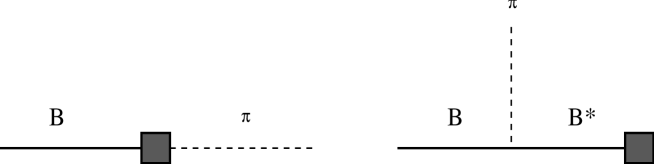
Figure 5: Tree diagrams for the $B\to\pi$ transition matrix element. The box represents the $b\to u$ weak current, the dashed line the pion.

At the leading order in $1/m_{Q}$ they give [10, 12]:

$$F_{1} = \frac{g{\hat{F}}\sqrt{M_{P}}}{2f_{\pi}(v\cdot p_{\pi}+\Delta_{P})}$$ (222)

$$F_{0} = \frac{{\hat{F}}}{f_{\pi}\sqrt{M_{P}}}~{}~{}.$$ (223)

The same relations have been obtained assuming $P^{*}$ pole dominance in [51], and in [124], combining PCAC and heavy quark spin symmetry. The formula (222) satisfies the asymptotic scaling (209): in the chiral limit $v\cdot p_{\pi}\to 0$, however, the scaling is modified as in (218), because $\Delta_{P}\sim 1/M_{P}$. The scaling at $q^{2}=0$ is easily derived from (215)

$$\frac{F_{1}^{B\pi}}{F_{1}^{D\pi}}\Big{|}_{(q^{2}=0)}\simeq\sqrt{\frac{M_{D}}{M_{B}}}$$ (224)

as in (216). Therefore, if we use the input $D\to K$ to fix the effective coupling $g{\hat{F}}$ in (222), we obtain the same results as in table 3, as expected.

Alternatively, one can take the estimates $g\approx 0.38$ (97) and ${\hat{F}}=0.30\pm 0.05$ GeV^3/2 (95), which give

$$F_{1}^{D\pi}(0) = \frac{{\hat{F}}g}{f_{\pi}\sqrt{M_{D}}}\simeq 0.63$$ (225)

$$F_{1}^{B\pi}(0) = \frac{{\hat{F}}g}{f_{\pi}\sqrt{M_{B}}}\simeq 0.38~{}~{}.$$ (226)

The uncertainties on these results, as arising from QCD sum rule approximations, can be estimated around $30\%$. We stress that at the charm scale the $1/m_{c}$ corrections are potentially relevant: nevertheless the prediction (225) is in rather good agreement with data. In table 4 we quote form factors and branching ratios obtained from (222), (223) and chiral symmetry.

Table 4: Predictions for semileptonic $D$ and $B$ decays in a pseudoscalar meson, in the effective lagrangian approach. We have neglected the $\eta~{}-\eta^{\prime}$ mixing. The branching ratios and the widths for $B$ must be multiplied for $|V_{ub}/0.0032|^{2}$. We assume $\tau_{B_{s}}=\tau_{B^{0}}=\tau_{B^{+}}=1.55~{}ps.$

Decay	$F_{1}(0)$	BR	Exp. data
$D^{0}\to\pi^{-}$	0.63	$2.4\cdot 10^{-3}$	$(3.9^{+2.3}_{-1.2})\cdot 10^{-3}$
$D^{+}\to\eta$	0.26	$4.9\cdot 10^{-4}$
$D_{s}\to\eta$	0.51	$2.3\cdot 10^{-2}$
$D_{s}\to K^{0}$	0.63	$3.0\cdot 10^{-3}$
$B^{0}\to\pi^{-}$	0.38	$1.6\cdot 10^{-4}$	$(1.63\pm 0.46\pm 0.34)\cdot 10^{-4}$
$B_{s}\to K$	0.38	$1.6\cdot 10^{-4}$

The effective lagrangian result (222) shows the dominance of the $P^{*}$ pole near the kinematic end-point. The $1/m_{Q}$ corrections to the leading results (225), (226) have been presented in [35], where it is shown that at the order $1/m_{Q}$ one has to introduce four new relevant couplings in the lagrangian and in the effective current. Two of the occurring parameters, $\rho_{1}$ and $\rho_{2}$, parameterize the $1/M$ corrections to the leptonic decay constants $f_{P}$ and $f_{P^{*}}$, as shown by (195). The others, $g_{1}$ and $g_{2}$, are related to the subleading corrections to the coupling $g_{P^{*}P^{*}\pi}$ and $g_{P^{*}P\pi}$, as shown in (49). In terms of these couplings, the form factor $F_{1}$ is [35]:

$$F_{1} = \frac{{\hat{F}}}{2\sqrt{M_{P}}f_{\pi}}\left[\frac{M_{P}+v\cdot p_{\pi}}{v\cdot p_{\pi}+\Delta}\left(1+\frac{\rho_{1}-2\rho_{2}}{M_{P}}\right)\left(g+\frac{g_{1}-g_{2}}{M_{P}}\right)-\left(1+\frac{\rho_{1}+2\rho_{2}}{M_{P}}\right)\right]$$ (227)

$$= \frac{1}{2f_{\pi}}\left(\frac{M_{P}+v\cdot p_{\pi}}{M_{P}(v\cdot p_{\pi}+\Delta)}g_{P^{*}P\pi}f_{P^{*}}-f_{P}\right)~{}~{},$$

where, in the second expression, $g_{P^{*}P\pi}$, $f_{P^{*}}$ and $f_{P}$ include their own $1/M$ corrections.

The chiral logarithmic corrections to the process $P\to\pi l\nu_{l}$ in the effective theory have been computed in [67]: evaluating the one-loop chiral diagrams, it is found that the chiral-corrected form factors $F_{1}$ and $F_{0}$ at the leading order in $1/m_{Q}$ have the same form as in (222), (223) but are expressed in terms of the chirally renormalized leptonic decay constants $f_{P}^{ren}$ and $f_{\pi}^{ren}$, the heavy meson coupling $g_{eff}$ to the axial vector Goldstone current (see also section 3.2) and the hyperfine mass splitting $\Delta^{ren}$, i.e.

$$F_{1} = \frac{g_{eff}f_{P}^{ren}M_{P}}{2f_{\pi}^{ren}(v\cdot p_{\pi}+\Delta_{P}^{ren})}$$ (228)

$$F_{0} = \frac{f_{P}^{ren}}{f_{\pi}^{ren}}~{}~{}.$$ (229)

A more detailed analysis is presented in [68], where all the non-analytic terms arising from chiral loops are kept. The $SU(3)$ violation in the pole term of the amplitude is of the order of $40\%$, but a rather large value of $g$ is used in the numerical estimate, $g\simeq 0.7$. For smaller values of $g$, e.g. $g=0.3$, the chiral violation between $P\to\pi$ and $P\to K$ pole amplitudes reduces to $10\%$.

5.3 $B\to V$ semileptonic decays

We now discuss the semileptonic decays of a heavy meson $P$ into a light vector meson $V=\rho$, $K^{*}$, $\phi$.

In the following, we will discuss how to relate the $B$ and $D$ form factors, following as before two different approaches: the scaling approach and the effective chiral lagrangian approach. Let us begin with a review of the available experimental data. In the $D\to K^{*}l\nu_{l}$ decay, the most extensively studied channel, the quality of the data does not yet allow to determine the $q^{2}$ dependence of the form factors. The analysis is performed assuming a simple pole formula for the form factors $V(q^{2}),\,A_{1}(q^{2})$, and $A_{2}(q^{2})$, with pole masses given by the nearest resonance (i.e. $2.1$ GeV for the vector form factor and $2.5$ GeV for the two axial form factors). The average of three Fermilab experiments gives the results [45]:

$$V(0)\;=\;1.1\pm 0.2;\;\;\;A_{1}(0)\;=\;0.56\pm 0.04;\;\;\;A_{2}(0)\;=\;0.40\pm 0.08.$$ (230)

Data have also been obtained for the decay $D_{s}\to\phi l\nu_{l}$, but the errors on the form factors are still large, and we shall not use them.

In the case of semileptonic $D$ decays, due to the limited $q^{2}$ range, the pole assumption does not sensibly affect the results (230); we have for instance extracted the form factors assuming $A_{1}$ constant in $q^{2}$, but $A_{2}$ and $V$ pole-dominated, finding discrepancies of the order of $10\%$, which are within the quoted uncertainties in (230). The $q^{2}$ dependence of the form factors is on the contrary extremely important in $B$ decays, as we discuss below.

For $B$ mesons the semileptonic rates are strongly Cabibbo-suppressed: the CLEO II Collaboration has only recently presented the new measurement giving [103]

$$BR(B^{0}\to\rho^{-}\ell^{+}{\nu}_{l}) = (3.88\pm 0.54\pm 1.01)\cdot 10^{-4}\;\;{\rm WSB}$$

$$BR(B^{0}\to\rho^{-}\ell^{+}{\nu}_{l}) = (2.28\pm 0.36\pm 0.59)\cdot 10^{-4}\;\;{\rm ISGW}$$ (231)

where the first value is obtained using the WSB model [105] in the Montecarlo code which evaluates the efficiencies, and the second one is based on the use of the ISGW model [106].

Before discussing semileptonic $B$ decays in more detail, let us stress that another source of information on the weak matrix elements between $B$ and $K$ or $K^{*}$ is represented by non leptonic $B$ decays. As a matter of fact, the factorization hypothesis allows to relate non-leptonic to semileptonic rates. The color-suppressed decays $B\to K(K^{*})J/\psi$ give, in this approximation, indications on the form factors $B\to K(K^{*})$ at $q^{2}=M^{2}_{J/\psi}$. There are two relevant experimental figures: the ratio of vector and pseudoscalar widths, measured by Argus [126] and CLEO II [125], whose averaged value is

$$R=\frac{\Gamma(B\to J/\psi K^{*})}{\Gamma(B\to J/\psi K)}=1.68\pm 0.33~{}~{},$$ (232)

and the fraction of longitudinal polarization

$$\frac{\Gamma_{L}}{\Gamma}=\frac{\Gamma(B\to J/\psi K^{*})_{L}}{\Gamma(B\to J/\psi K^{*})}=0.74\pm 0.07~{}~{},$$ (233)

which corresponds to the average of the measurements of Argus: $\Gamma_{L}/\Gamma=0.97\pm 0.16\pm 0.15$ [126], CLEO II: $\Gamma_{L}/\Gamma=0.80\pm 0.08\pm 0.05$ [125], and CDF: $\Gamma_{L}/\Gamma=0.65\pm 0.10\pm 0.04$ [127].

Detailed phenomenological analyses have been performed in [119, 120, 121], where it has been shown that most of the models fail to explain the previous data, in particular the fraction of longitudinal polarization (233). We point out that all the current models use the hypothesis of factorization [128], which in general works satisfactorily in $B$ decays [129] but could have corrections in specific channels, like the colour-suppressed $B\to J/\psi K^{*}$. Possible non-factorizable contributions are introduced in [130].

By the definition

$$x=\frac{A_{2}^{BK^{*}}}{A_{1}^{BK^{*}}}\Big{|}_{(M^{2}_{J/\psi})}~{}~{}~{}~{}~{}~{}~{}~{}y=\frac{V^{BK^{*}}}{A_{1}^{BK^{*}}}\Big{|}_{(M^{2}_{J/\psi})}$$ (234)

one gets, assuming factorization [119],

$$R=1.081\left(\frac{A_{1}^{BK^{*}}}{F_{1}^{BK}}(M^{2}_{J/\psi})\right)^{2}\left[(a-bx)^{2}+2(1+cy^{2})\right]$$ (235)

$$\frac{\Gamma_{L}}{\Gamma}=\frac{(a-bx)^{2}}{(a-bx)^{2}+2(1+cy^{2})}~{}~{}.$$ (236)

The coefficients $a$, $b$ and $c$ are dimensionless combinations of masses; from the data one gets

$$a=3.16~{}~{}~{}~{}b=1.31~{}~{}~{}~{}c=0.19~{}~{}.$$ (237)

5.3.1 Scaling approach to $B\to V$ form factors

The scaling approach, valid at the leading order in $1/m_{Q}$, is similar to the case $P\to\pi$; the scaling laws for the form factors are derived from the asymptotic behaviour of the matrix element, i.e.

$$<V(p^{\prime})|J_{\mu}|P(v)>\sim\sqrt{m_{Q}}\left(1+{\cal O}\left(\frac{\Lambda_{QCD}}{m_{Q}}\right)+{\cal O}\left(\frac{v\cdot p^{\prime}}{m_{Q}}\right)+{\cal O}\left(\frac{m_{V}}{m_{Q}}\right)\right)~{}~{}.$$ (238)

For $D\to K^{*}$ the violation to (238) can be important, namely of order $m_{K^{*}}/M_{D}$. This uncertainty is reflected in different choices of the scaling laws at $q^{2}\simeq q^{2}_{max}$. For example one can follow the approach called “soft-scaling” in [120], and adopted in [15], i.e.

$$V(q^{2}_{max}) \approx \frac{M_{P}+M_{V}}{\sqrt{M_{P}}}$$

$$A_{1}(q^{2}_{max}) \approx \frac{\sqrt{M_{P}}}{M_{P}+M_{V}}$$

$$A_{2}(q^{2}_{max}) \approx \frac{M_{P}+M_{V}}{\sqrt{M_{P}}}~{}~{}.$$ (239)

The second choice we shall consider is “hard-scaling”:

$$V(q^{2}_{max}) \approx \sqrt{M_{P}}$$

$$A_{1}(q^{2}_{max}) \approx \frac{1}{\sqrt{M_{P}}}$$

$$A_{2}(q^{2}_{max}) \approx \sqrt{M_{P}}~{}~{}.$$ (240)

The two scenarios, (239) and (240), differ by subleading terms of the order $M_{V}/M_{P}$, which can be nevertheless numerically important. Needless to say, some form factors might exhibit soft-scaling and others hard-scaling, in different combinations.

The scaling laws allow to relate the $D$ and $B$ form factors near $q^{2}_{max}$: as discussed above, the dependence on $q^{2}$ is practically unknown, and, as we stressed already, $B$ transitions depend strongly on the extrapolation to $q^{2}=0$. The vector form factor $V$ is generally believed to be pole-dominated, as discussed in section 5.1, while for $A_{1}$ and $A_{2}$ the theoretical situation is unclear. In [120] the soft scaling laws are justified by extending the heavy-to-heavy scaling relations down to the light final meson case. In the same limit one finds that $A_{2}/A_{1}$, $V/A_{1}$ and $F_{1}/A_{1}$ should have a polar behaviour in $q^{2}$: assuming $F_{1}$ as pole dominated, this implies a constant $A_{1}$ and a pole behaviour for $A_{2}$ and $V$. Nevertheless the extension of the heavy-to-heavy scaling laws to the heavy-to-light case remains arbitrary, and should be considered as an ansatz. As we will discuss explicitly in the next section, the effective lagrangian approach leads to the soft-scaling solution (239): this follows from the factor $(M_{P}+M_{V})$ contained in the definition (200) of the form factors.

To simplify the discussion, we assume that $A_{2}$ is dominated by the nearest pole, while for $A_{1}$ we consider two possibilities: the pole-dominance, and a flat $A_{1}$ constant in $q^{2}$. We have considered four different possible scenarios: soft scaling and $A_{1}$ pole-dependent (called soft-pole), soft scaling and $A_{1}$ constant (called soft-constant), hard scaling and $A_{1}$ pole-dependent (called hard-pole), and finally hard scaling and $A_{1}$ constant (called hard-constant). For each of them we have computed, using as inputs the $D\to K^{*}$ form factors (230), the branching fraction and the ratios of decay widths $\Gamma_{+}/\Gamma_{-}$ and $\Gamma_{L}/\Gamma_{T}$ for the process $B^{0}\to\rho^{-}l^{+}\nu_{l}$. Here $\Gamma_{T}$ and $\Gamma_{L}$ refer to $\rho$ with transverse and longitudinal polarization respectively, $\Gamma_{+}$ and $\Gamma_{-}$ to $\rho$ with positive and negative helicities. We have computed the longitudinal fraction $\Gamma_{L}/\Gamma$, and the ratio of the vector to scalar BR’s for $B\to J/\psi K(K^{*})$. The results are presented in table 5, where we have extrapolated from $D\to K^{*}$ to $B\to K^{*}$, and then we have equated, by chiral symmetry, the form factors $B\to K^{*}$ and $B\to\rho$.

Table 5: Predictions for form factors and widths for $B^{0}\to\rho^{-}l\nu_{l}$. $\Gamma_{T}$ and $\Gamma_{L}$ refer to $\rho$ with respectively transverse and longitudinal polarization, $\Gamma_{+}$ and $\Gamma_{-}$ to $\rho$ with positive and negative helicities. The branching ratios (BR) and the widths for $B$ must be multiplied for $|V_{ub}/0.0032|^{2}$. We assume $\tau_{B_{s}}=\tau_{B^{0}}=\tau_{B^{+}}=1.55~{}ps.$

Extrapolation	soft-pole	hard-pole	soft-cost.	hard-cost.	data
$A_{1}(0)$	0.21	0.17	0.42	0.33
$A_{2}(0)$	0.27	0.34	0.27	0.34
$V(0)$	0.64	0.81	0.64	0.81
${\Gamma_{+}}/{\Gamma_{-}}$	0.045	0.13	0.005	0.06
${\Gamma_{L}}/{\Gamma_{T}}$	0.39	0.15	1.80	0.30
BR ($10^{-4}$)	2.8	2.8	6.7	3.5	$3.88\pm 0.54\pm 1.01$
${\Gamma_{L}}/{\Gamma}(J/\psi K^{*})$	0.27	0.02	0.50	0.18	$0.74\pm 0.07$
${\Gamma(K^{*})}/{\Gamma(K)}$	1.74	1.68	3.35	2.27	$1.68\pm 0.33$

Let us comment on table 5. First of all, all the four scenarios give a rather low value for the ratio $\Gamma_{L}/\Gamma(J/\psi K^{*})$: the soft-scaling, $A_{1}$ constant (third column of table 5), is the closest one to the experiment, but it produces a too high value for the branching ratio $B\to\rho^{-}l\nu_{l}$ and for $\Gamma(K^{*})/\Gamma(K)$. The value of the latter ratio depends mainly on the ratio $A_{1}/F_{1}$ (at $q^{2}=M^{2}_{J/\psi}$), and could be smaller for a larger value of $F_{1}^{B\;K}$: however, a too large value would disagree with the measured branching ratio for the $B\to\pi l\nu_{l}$ (excluding large $SU(3)$ violation). This scenario is preferred in [120], where however the upper limit for the $B\to\rho$ and the $B\to\pi$ data are not taken into account (soft-scaling is also applied to $F_{1}$, obtaining a larger value for it and a better agreement for $\Gamma(K^{*})/\Gamma(K)$).

The second comment is that a constant $A_{1}$ gives a higher value than pole behaviour for the $B\to\rho$ branching ratio, when scaling is used. The situation improves assuming pole dominance for $A_{1}$ for the semileptonic branching ratio $B\to\rho$, and also for the ratio $\Gamma(K^{*})/\Gamma(K)$, as it can be seen in the first column of the table. But, at the same time, the longitudinally polarized fraction $\Gamma_{L}/\Gamma(J/\psi\;K^{*})$ decreases, because $A_{2}/A_{1}$ at $q^{2}=M^{2}_{J/\psi}$ grows.

Hard scaling decreases the value of $A_{1}$, and it raises $A_{2}$ and $V$: this produces a smaller semileptonic $BR(B\to\rho)$, but also lowers $\Gamma_{L}/\Gamma(J/\psi\;K^{*})$ (because $A_{2}/A_{1}$ grows, see (236)) and $\Gamma(K^{*})/\Gamma(K)$. Hard scaling, together with a pole-dominated $A_{1}$, as in the second column, leads to a value for $\Gamma_{L}/\Gamma(J/\psi\;K^{*})$ in disagreement with the data: its combination with a constant $A_{1}$, as in the fourth column of the table, improves the agreement with the data, even if $\Gamma_{L}/\Gamma(J/\psi\;K^{*})$ remains still rather small, even smaller than in soft-pole scenario for $A_{1}$.

Summarizing, the previous analysis indicates that a constant $A_{1}$ requires strong scaling in order to get agreement with the data of the semileptonic $BR(B\to\rho)$. In [120] a different result is obtained, which, however, does not take into account the results for the semileptonic $B\to\rho$ transition.

If $A_{1}$ is single-pole dominated, soft scaling is required in order to get a reasonable (not too small) value for $\Gamma_{L}/\Gamma(J/\psi\;K^{*})$: these data are however difficult to explain without spoiling other phenomenological requests.

It should be stressed, however, that the figures of table 5 have large uncertainties. Leaving aside theoretical uncertainties that are however significant, the quoted numbers have an uncertainty due to the experimental errors of the $D\to K^{*}l\nu_{l}$ form factors (230) used as inputs. We notice that, for instance, $A_{2}(0)^{D\;K^{*}}$ is quoted with an error of about 20 %: this error alone implies 30 % uncertainty in $\Gamma_{L}/\Gamma(J/\psi\;K^{*})$ and 15 % in $\Gamma(K^{*})/\Gamma(K)$. Finally we have used flavour $SU(3)$ symmetry to relate $B\to\rho$ and $B\to K^{*}$ form factors and this is another source of theoretical error which in principle should be taken into account.

5.3.2 Effective lagrangian approach

Light vector resonances have been discussed in the framework of the effective heavy meson chiral lagrangian in 2.4; applications to semileptonic decays have been developed in [15]. Chiral loop contributions to $D\to K^{*}l\nu_{l}$ have been partially taken into account in [38]. We now review this subject.

In the effective chiral lagrangian framework, five different diagrams contribute at the leading order in $1/m_{Q}$ to the matrix element $<V(p^{\prime},\epsilon)|J_{\mu}|P(p)>$. They are analogous to the diagrams of fig. 5. Four of them are polar diagrams: $V(q^{2})$ takes contribution from the $1^{-}$ pole diagram, proportional to the coupling $\lambda$ among $P$, $P^{*}$ and $\rho$ introduced in (60). The $\zeta$ and $\mu$ couplings in (74) give the vertex $PP^{**}\rho$, where $P^{**}$ is a positive-parity states of the doublet $(0^{+},1^{+})$ and the corresponding polar diagrams, with exchange of a $1^{+}$ meson, contribute to $A_{1}$ and $A_{2}$. The $\mu$ and $\lambda$ terms have dimension higher than the $\zeta$ or $g$ terms; nevertheless they are the lowest-order contributions to $V$ and $A_{2}$. The fourth polar diagram, with exchange of a $0^{-}$ meson, is proportional to the coupling $\beta$ of the vertex $PP\rho$ (see formula (60)) and is relevant only for the form factor $A_{0}$. Finally there is a direct diagram, which arises from the effective current term proportional to $\alpha_{1}$ in the heavy-to-light current (182). All these vertices can be found in appendix A.

Computing the diagrams for $q^{2}\simeq q^{2}_{max}$ and at leading order in $1/m_{Q}$, one gets [15]:

$$V(q^{2}_{\rm max})=\frac{g_{V}}{\sqrt{2}}\lambda{\hat{F}}\frac{M_{P}+M_{V}}{\sqrt{M_{P}}}\frac{1}{M_{V}+\Delta_{P^{*}P}}$$ (241)

$$A_{1}(q^{2}_{\rm max})=-\frac{2g_{V}}{\sqrt{2}}\frac{\sqrt{M_{P}}}{M_{P}+M_{V}}\left[\alpha_{1}-\frac{{\hat{F}}^{+}(\zeta/2-\mu M_{V})}{M_{V}+\Delta_{PP^{**}}}\right]$$ (242)

$$A_{2}(q^{2}_{\rm max})=-\frac{\mu g_{V}{\hat{F}}^{+}}{\sqrt{2}(M_{V}+\Delta_{PP^{**}})}\frac{M_{P}+M_{V}}{\sqrt{M_{P}}}$$ (243)

$$A_{0}(q^{2}_{\rm max})=\frac{g_{V}}{2\sqrt{2}}\frac{\beta{\hat{F}}\sqrt{M_{P}}}{M_{V}(M_{V}+\Delta^{\prime})}+\frac{g_{V}}{\sqrt{2}}\frac{\alpha_{1}\sqrt{M_{P}}}{M_{V}}$$ (244)

where the $\Delta$ are appropriate mass splittings.

From (241)-(244), we can extract information on the scaling behaviour of the form factors as well as some indications on their $q^{2}$ behaviour.

As to the scaling, we notice that (241)-(243) imply the “soft-scaling” of eq. (239), since the coupling of the effective lagrangian is flavour independent. Moreover, the form factors $V$ and $A_{2}$ have only the pole structure, which at $q^{2}\simeq q^{2}_{\rm max}$ is signalled by the factor $1/(M_{V}+\Delta)$, while $A_{1}$ contains a pole term but also a non-polar one, proportional to $\alpha_{1}$. This suggests a more complex $q^{2}$ behaviour of $A_{1}$.

The non-polar term could be a general polynomial in $q^{2}$: the simplest way to take into account the indications coming from the effective lagrangian is to describe $A_{1}$ as a sum of a constant term and a pole term, i.e. we write:

$$A_{1}(q^{2})=a+\frac{b}{1-q^{2}/M^{2}_{P^{**}}}$$ (245)

while keeping for $A_{2}$ and $V$ the nearest-pole behaviour. The parameters $a$ and $b$ are flavour dependent, and scale differently at $q^{2}=q^{2}_{\rm max}$. Assuming soft scaling, as suggested by (241) - (244), we find the following scaling laws:

$$a(B\to V) = \frac{M_{D}+M_{V}}{M_{B}+M_{V}}\sqrt{\frac{M_{B}}{M_{D}}}a(D\to V)$$ (246)

$$b(B\to V) = \frac{M_{D}+M_{V}}{M_{B}+M_{V}}\sqrt{\frac{M_{D}}{M_{B}}}b(D\to V)~{}~{}.$$ (247)

The formulas (241)-(243) give the form factors at $q^{2}_{\rm max}$: at the leading order in $1/m_{Q}$, the value in $q^{2}=0$ for pole-dominated terms is:

$$F(0)=\frac{2(M_{V}+\Delta)}{M_{P}}F(q^{2}_{\rm max})~{}~{}.$$ (248)

As for $A_{1}$, we identify the term proportional to $\alpha_{1}$ in (242) with the constant term $a$ of (245), and the other with the pole term, proportional to $b$. In this way one gets:

$$V(0)=g_{V}\sqrt{2}\lambda{\hat{F}}\frac{M_{P}+M_{V}}{M_{P}^{3/2}}$$ (249)

$$a=-g_{V}\sqrt{2}\frac{\sqrt{M_{P}}}{M_{P}+M_{V}}\alpha_{1}$$ (250)

$$b=g_{V}2\sqrt{2}{\hat{F}}^{+}\frac{\zeta/2-\mu M_{V}}{(M_{P}+M_{V})\sqrt{M_{P}}}$$ (251)

$$A_{2}(0)=-\sqrt{2}\mu g_{V}{\hat{F}}^{+}\frac{M_{P}+M_{V}}{M_{P}^{3/2}}~{}~{}.$$ (252)

From the experimental data (230) on $D\to K^{*}$ we can fix the effective couplings appearing in the previous formulas: from (249), using ${\hat{F}}=0.30\;GeV^{3/2}$ and $g_{V}=5.8$ (see (65)), we obtain

$$|\lambda|=0.41\;GeV^{-1}~{}~{}.$$ (253)

We shall see, in the next section, how the sign of $\lambda$ can be fixed. It is interesting to observe that this result agrees with the second, but not with the first determination obtained in [131] by a light cone sum rules calculation (the first determination gives a higher value; also in [132] a higher value of $\lambda$ is obtained).

Similarly, from (252) and ${\hat{F}}^{+}=0.46\;GeV^{3/2}$ [79] we get

$$\mu=-0.10\;GeV^{-1}~{}~{}.$$ (254)

Having fixed $\lambda$ and $\mu$, one can compute the form factors $V$ and $A_{2}$ for the $B\to K^{*}$ and $B\to\rho$ matrix elements, because these couplings are heavy-flavour independent at the leading order. The result is

$$|V^{B\to V}(0)|=0.50~{}~{}~{}~{}~{}~{}~{}~{}~{}~{}A_{2}^{B\to V}(0)=0.19~{}~{}.$$ (255)

The mass difference between $K^{*}$ and $\rho$ is numerically irrelevant in (255).

Concerning $A_{1}$, from the input $A_{1}^{D\;K^{*}}(0)$, we derive

$$(a+b)^{D\;K^{*}}=0.56~{}~{}.$$ (256)

The knowledge of the $q^{2}$ behaviour of $A_{1}^{D\;K^{*}}$ would allow to extract simultaneously $a$ and $b$, but at present we can only introduce an arbitrary parameter $r$, defined as

$$r=\frac{a}{a+b}$$ (257)

where $a$ and $b$ are relative to the $A_{1}^{D\to K^{*}}$ ($r$ is not heavy flavour independent).

When $r$ varies from $r=0$ to $r=1$, we have a smooth transition from a pure pole dominance ($r=0$) to a constant $A_{1}$ ($r=1$). The analysis of section 5.3.1 has shown that a pure pole behaviour (soft-pole case) leads to a rather low value for $\Gamma_{L}/\Gamma(J/\psi\;K^{*})$, while a constant $A_{1}$ gives a semileptonic branching ratio $B\to\rho$ too high: therefore we expect that the two component form factor (245) can explain better, for some intermediate value of $r$, the large longitudinal polarization in $B\to J/\psi K^{*}$ and at the same time can agree with the data for $B\to\rho l\nu$.

In figs. 6, 7 and 8 we plot respectively $\Gamma_{L}/\Gamma(J/\psi\;K^{*})$, $\Gamma(K^{*})/\Gamma(K)$ and $BR(B^{0}\to\rho^{-}l^{+}\nu_{l})$ as a function of $r$. We have assumed $A_{2}$ and $V$ pole-dominated, with the values (255) at $q^{2}=0$. We see that all the three observables grow when the $q^{2}$ dependence of $A_{1}$ becomes flatter, i.e. $r\to 1$. This is a satisfactory feature for $\Gamma_{L}/\Gamma(J/\psi\;K^{*})$, but a large $r$ gives too large values for the semileptonic $BR$ and for the $\Gamma(K^{*})/\Gamma(K)$ ratio.

Figure 6: Ratio $\Gamma_{L}/\Gamma$ for the decay $B\to J/\psi K^{*}$ as a function of the parameter $r$. $\Gamma_{L}$ is the width for longitudinally polarized $K^{*}$.

Figure 7: Ratio of the widths $B\to J/\psi K^{*}$ and $B\to J/\psi K$ as a function of the parameter $r$.

Figure 8: Branching ratio of the decay $B^{0}\to\rho^{-}l\nu_{l}$ as a function of the parameter $r$. We have taken $V_{ub}=0.0032$.

In table 6 we quote the values of various observables at $r=0.5$, where a good compromise is obtained: $\Gamma_{L}/\Gamma(J/\psi\;K^{*})=0.51$. This value is still smaller than the data, but one should not forget that the factorization assumption could receive sizeable corrections.

Table 6: Predictions for form factors and widths for $B^{0}\to\rho^{-}l\nu_{l}$ and for $B\to J/\psi K^{(*)}$, with $r=0.5$. $\Gamma_{T}$ and $\Gamma_{L}$ refer to $\rho$ with, respectively, transverse and longitudinal polarization, $\Gamma_{+}$ and $\Gamma_{-}$ to $\rho$ with positive and negative helicities. The branching ratios (BR) and the widths for $B$ must be multiplied for $|V_{ub}/0.0032|^{2}$. We assume $\tau_{B_{s}}=\tau_{B^{0}}=\tau_{B^{+}}=1.55~{}ps.$

Observable	r = 0.5	data
$A_{1}(0)$	0.28
$A_{2}(0)$	0.19
$V(0)$	0.50
${\Gamma_{+}}/{\Gamma_{-}}$	0.013
${\Gamma_{L}}/{\Gamma_{T}}$	1.60
BR ($10^{-4}$)	3.8	$3.88\pm 0.54\pm 1.01$
${\Gamma_{L}}/{\Gamma}(J/\psi K^{*})$	0.51	$0.74\pm 0.07$
${\Gamma(K^{*})}/{\Gamma(K)}$	2.01	$1.68\pm 0.33$

From the value of $r$ one can extract $a$ and $b$ separately: from the scaling relations (246) and (247) we have for $r=0.5$:

$$a(B\to V)=0.21~{}~{}~{}~{}~{}~{}~{}~{}~{}~{}~{}~{}~{}~{}b(B\to V)=0.07$$ (258)

i.e. $A_{1}^{B\rho}(0)=0.28$, as quoted in table 6. The knowledge of $a$ and $b$, together with the identifications (250) and (251), fixes the couplings $\alpha_{1}$ and the linear combination $\zeta/2-\mu M_{V}$. The results depend on the value of $r$; for $r=0.5$ we get:

$$\alpha_{1}=-0.07\;GeV^{1/2}\hskip 56.9055pt\frac{\zeta}{2}-\mu M_{V}=0.14$$ (259)

($a$ and $b$ are taken as positive). From (254) we can extract finally $\zeta$:

$$\zeta=0.10~{}~{}.$$ (260)

The previous phenomenological analysis has to be taken cautiously, due to the large uncertainties. Subleading corrections, $q^{2}$ dependence of the form factors, breaking of factorization and chiral violations could easily lead to substantial modifications of the chosen scenario. New experimental data will hopefully clarify the situation, and allow to distinguish among different models. We shall adopt in the following the effective lagrangian results of table 6 (in particular $r=0.5$).

In table 7 we present the values of the form factors of the $b\to u$ transitions in different models.

Table 7: Form factors at $q^{2}=0$ for $b\to u$ transitions in different models

Reference	$F_{1}^{B\to\pi}$	$A_{1}^{B\to\rho}$	$A_{2}^{B\to\rho}$	$V^{B\to\rho}$
This paper	$0.38$	$0.28$	$0.19$	$0.50$
QCD sum rules
DP [54]	$0.4\pm 0.1$
CZ [133]	$0.36$
BBD [107]	$0.24\pm 0.025$
Narison [134]	$0.23\pm 0.02$	$0.35\pm 0.16$	$0.42\pm 0.12$	$0.47\pm 0.14$
Ball [108]	$0.26\pm 0.02$	$0.5\pm 0.1$	$0.4\pm 0.2$	$0.6\pm 0.2$
BKR [109]	$0.24-0.29$
ABS [110]		$0.24\pm 0.04$		$0.28\pm 0.06$
Quark models
BSW [105]	$0.33$	$0.28$	$0.28$	$0.33$
ISGW [106]	$0.09$	$0.05$	$0.0.02$	$0.27$
FGM [135]	$0.21\pm 0.02$	$0.26\pm 0.03$	$0.30\pm 0.03$	$0.29\pm 0.03$
Lattice
APE [116]	$0.35\pm 0.08$	$0.24\pm 0.12$	$0.27\pm 0.80$	$0.53\pm 0.31$
Abada et al. [114]	$0.30\pm 0.14\pm 0.05$	$0.22\pm 0.05$	$0.49\pm 0.21\pm 0.05$	$0.37\pm 0.11$
UKQCD [118]		$0.27^{+7+3}_{-4-3}$

6 Radiative decays

6.1 Flavour conserving radiative decays: $D^{*}\to D\gamma$

In this section we shall consider the decay

$$D^{*}_{a}\to D_{a}\gamma\hskip 3.0pt,$$ (261)

and the related processes for the $B$ case: $B^{*}_{a}\to B_{a}\gamma$. In (261) $a=1,2,3$ is the light quark index corresponding to $u,d,s$. The matrix element for this radiative transition is as follows:

$${\cal M}(D^{*}_{a}\to D_{a}\gamma)=\hskip 3.0pti\,e\mu_{a}\epsilon^{\mu\nu\alpha\beta}\epsilon^{*}_{\mu}\eta_{\nu}p_{\alpha}p^{\prime}_{\beta}\hskip 3.0pt.$$ (262)

In (262) $\epsilon_{\mu}$ is the photon polarization, whereas the coupling $\mu_{a}$ comprises two terms:

$$\mu_{a}=\mu_{a}^{\ell}+\mu_{a}^{h}~{}~{},$$ (263)

corresponding to the decomposition:

$${\cal M}(D^{*}_{a}\to D_{a}\gamma)=e\;\epsilon^{*\mu}\;<D_{a}(p^{\prime})|J_{\mu}^{em}|D^{*}_{a}(p,\eta)>=e\;\epsilon^{*\mu}\;<D_{a}(p^{\prime})|J_{\mu}^{\ell}+J_{\mu}^{h}|D^{*}_{a}(p,\eta)>~{}~{}.$$ (264)

Here $J_{\mu}^{\ell}$ and $J_{\mu}^{h}$ are the light and the heavy quark parts of the electromagnetic current:

$$J_{\mu}^{\ell}=\frac{2}{3}\bar{u}\gamma_{\mu}u-\frac{1}{3}\bar{d}\gamma_{\mu}d-\frac{1}{3}\bar{s}\gamma_{\mu}s=\sum_{a=1}^{3}e_{a}\bar{q}_{a}\gamma_{\mu}q_{a}$$ (265)

and

$$J_{\mu}^{h}=\frac{2}{3}\bar{c}\gamma_{\mu}c-\frac{1}{3}\bar{b}\gamma_{\mu}b=\sum_{Q=c,b}e_{Q}\bar{Q}\gamma_{\mu}Q.$$ (266)

Correspondingly, eq. (263) becomes

$$\mu_{a}=\mu_{a}^{\ell}+\mu_{a}^{h}=\frac{e_{a}}{\Lambda_{a}}+\frac{e_{Q}}{\Lambda_{Q}}~{}~{},$$ (267)

where $\Lambda_{a}$ and $\Lambda_{Q}$ are mass parameters to be determined.

Let us consider the two currents $J_{\mu}^{h}$ and $J_{\mu}^{\ell}$ separately. The matrix element of $J_{\mu}^{h}$ can be obtained from the Lagrange density:

$${\cal L}^{\prime\prime}=-{e\over 2m_{Q}}e_{Q}{\bar{h}}_{v}\sigma^{\mu\nu}h_{v}F_{\mu\nu}\hskip 5.0pt,$$ (268)

which allows the transition $Q\to Q\gamma$ and can be expressed in terms of the Isgur-Wise universal form factor $\xi(v\cdot v^{\prime})$ as follows:

$$<D_{a}(p^{\prime})|J_{\mu}^{h}|D_{a}^{*}(p,\eta)>=\,e_{c}<D_{a}(p^{\prime})|\bar{c}\gamma^{\mu}c|D_{a}^{*}(p,\eta)>=i\frac{2}{3}\sqrt{M_{D_{a}}M_{D_{a}^{*}}}\xi(v\cdot v^{\prime})\epsilon_{\mu\nu\alpha\beta}\eta^{\nu}v^{\alpha}v^{\prime\beta}\hskip 3.0pt,$$ (269)

where $p^{\prime}=M_{D}v^{\prime}$, $p=M_{D^{*}}v$ and $v\cdot v^{\prime}\simeq 1$ because:

$$0=q^{2}=m^{2}_{D}+M_{D^{*}}^{2}-2M_{D}M_{D^{*}}v\cdot v^{\prime}\hskip 3.0pt.$$ (270)

Taking into account the normalization of $\xi(v\cdot v^{\prime})$: $\xi(1)=1$, one gets, for the charm case,

$$\mu_{a}^{h}\;=\;\frac{2}{3\Lambda_{c}}$$ (271)

($\mu_{a}^{h}\;=\;-\;\frac{1}{3\Lambda_{b}}$ for the $b$ case), with

$$\Lambda_{c}={\sqrt{M_{D_{a}}M_{D^{*}_{a}}}}$$ (272)

(resp. $\Lambda_{b}={\sqrt{M_{B_{a}}M_{B^{*}_{a}}}}$); in the leading order in $1/m_{c}$ one finds:

$$\Lambda_{c}\;=\;m_{c}$$ (273)

(resp. $\Lambda_{b}\;=\;m_{b}$), independently of the light quark label $a$.

Let us now consider the second term in (263), i. e. $\mu_{a}^{\ell}$, which cannot be computed within HQET since it involves light quarks; we shall now show that the chiral effective theory can be employed to get information on this quantity. We shall examine two approaches: the first one is based on the calculation of chiral loop corrections [47]; the second is based on the use of Vector Meson Dominance (VMD), together with the effective chiral lagrangian for light and heavy mesons [136]. Other approaches used to compute (261) are based on quark models [49, 27, 137]; bag model [138] and QCD sum rules [139, 140] (for a previous review of theoretical results see [141]).

The first approach we consider is based on the chiral loop corrections to the tree diagram [47]. Let us start with the definition of $\mu_{a}^{\ell}$:

$$\mu_{a}^{\ell}\;=\;\frac{e_{a}}{\Lambda_{a}}\;;$$ (274)

in the limit of $SU(3)$ symmetry the constants ${\Lambda_{a}}$’s are equal, i. e. one gets ${\Lambda_{a}}^{-1}\;=\;\beta$, where $\beta$ is an unknown constant which can also contain effects suppressed by powers of $1/m_{c}$.

The leading $SU(3)$ violations to (274) are obtained by considering the loop diagrams of fig. 9, with the results [47]:

$$\mu_{1}^{\ell}=\frac{2}{3}\beta-g^{2}\frac{m_{K}}{4\pi f_{K}^{2}}-g^{2}\frac{m_{\pi}}{4\pi f_{\pi}^{2}}$$ (275)

$$\mu_{2}^{\ell}=-\frac{1}{3}\beta+g^{2}\frac{m_{\pi}}{4\pi f_{\pi}^{2}}$$ (276)

$$\mu_{3}^{\ell}=-\frac{1}{3}\beta+g^{2}\frac{m_{K}}{4\pi f_{K}^{2}}~{}~{}.$$ (277)

Here $g$ is the strong coupling constant of the vertex $D^{*}D\pi$ (in the $m_{c}\to\infty$ limit) defined in (38). If one considers only the leading $SU(3)$ violations, one should put $f_{K}=f_{\pi}$. This has to be the case if one uses the value $g=0.38$, eq. (97). As a matter of fact, as discussed in [72], the $SU(3)$ invariant coupling $g$ is obtained assuming a unique value $f_{\pi}\approx 130MeV$ for all the light pseudoscalar meson decay constants in the sum rule.

Figure 9: Chiral loops contributing to the radiative decays $D^{*}\to D\gamma$

The analysis of [47] provides a pattern for $SU(3)$ violations in $D^{*}$ radiative decays, and can be in principle used to determine $g$ and $\beta$, independently of the theoretical determinations based on the the QCD sum rule for $g$. One can use the two formulas:

$$\Gamma(D^{*}_{a}\to D_{a}\gamma)=\frac{\alpha}{3}\frac{M_{D^{*}_{a}}}{M_{D_{a}}}|\mu_{\alpha}|^{2}|{\vec{k}}|^{3}$$ (278)

(${\vec{k}}$ = photon momentum),

$$\Gamma(D^{*+}\to D^{0}\pi^{+})=\frac{g^{2}}{6\pi f_{\pi}^{2}}|{\vec{p}_{\pi}}|^{3}$$ (279)

and the experimental results contained in table 1 [44, 45], together with the condition $g<1$ (which is experimentally satisfied [46]). Because of the large experimental error (especially in the channel $D^{*+}\to D^{+}\gamma$), one gets, however, a rather broad range of values for $g$ [47]:

$$0.3<g<0.7~{}~{}.$$ (280)

The value of $g$ obtained in this way is an effective coupling which takes into account part of the $1/m_{c}$ corrections, as it is obvious from the fact that $\mu_{a}^{h}$ has not been neglected in comparison with $\mu_{a}^{\ell}$ ($\mu_{a}^{h}$ is not negligible because $m_{c}$ is not sufficiently large: in this analysis one uses $\Lambda_{c}=m_{c}=1.7$ GeV). It is nevertheless interesting to observe that the small values for $g$ in (280) are in broad agreement with the results of the QCD sum rules quoted in section 3.1.2.

The analysis of [47] shows that smaller values of $g$ favour values of $\beta$ near the non relativistic quark model result [137], where $\beta=m_{q}^{-1}$, and $m_{q}\approx 300-500~{}MeV$ is a typical value of the light quark constituent mass. In particular, from $g=0.38$ and $m_{c}=1.7$ GeV one gets the value $\beta=1.9$ GeV^-1. The pattern displayed by eq.(277), $\mu_{3}^{\ell}=-\frac{1}{3}(\beta-3g^{2}{m_{K}}/(4\pi f_{K}^{2}))$ $=-{1}/(3\Lambda_{3})$, can be interpreted, in the quark model, as due to a constituent strange quark having a mass $m_{s}={\Lambda_{3}}$ larger than $m_{q}=\Lambda_{1}$, or $\Lambda_{2}$, which is what one would naively expect.

Instead of considering loop effects one can therefore take into account $SU(3)$ violations by choosing explicitly different $\Lambda_{a}$’s. Quark model calculations that assume $SU(3)$ violations are considered in [49, 27]. In particular, the calculation of ref. [27] in the semirelativistic quark model of ref. [57] discussed in section 3.1.1, as we stated already, makes use of the Salpeter equation [56], i.e. a wave equation which takes into account relativistic kinematics, with an interquark potential modelled on the Richardson’s potential [55]. As we have observed, this model is able to explain the reduction of the value of the strong ${D^{*}D\pi}$ coupling constant from the (non relativistic) quark model prediction $g=1$ down to $g\approx 0.33$, as a consequence of the relativistic kinematics relevant to the light quark in the heavy meson; since this small value is favoured by the QCD sum rule analyses [25, 60], as well as by the data (eq.(280)) one may take this as an indication that relativistic kinematics plays a role also in the case of the radiative decays. The results of the analysis in [27] for the constants $\Lambda_{a}$ are displayed in table 8, together with the results of the chiral loop calculation [47], i.e. the results based on eqs. (275)-(277). In the same table we also report the parameters of the model [136] based on Vector Meson Dominance, to be discussed below.

Table 8: Theoretical inputs for mass parameters in radiative D decays. $\chi$-loop represents the chiral loop calculation, VMD is the model based on the effective lagrangian supplemented by the hypothesis of Vector Meson Dominance; RQM refers to the relativistic quark model; $\Lambda_{Q}$ and $\Lambda_{a}$ are mass parameters (in GeV).

Decay mode	$\chi$-loop		VMD		RQM
	$\Lambda_{Q}$	$\Lambda_{a}$	$\Lambda_{Q}$	$\Lambda_{a}$	$\Lambda_{Q}$	$\Lambda_{a}$
$D^{*+}\to D^{+}\gamma$	1.7	0.61	1.9	0.50	1.57	0.48
$D^{*0}\to D^{0}\gamma$	1.7	0.79	1.9	0.50	1.57	0.48
$D^{*}_{s}\to D_{s}\gamma$	1.7	1.11	2.0	0.59	1.58	0.497
$B^{*+}\to B^{+}\gamma$	5.0	0.79	5.3	0.51	4.93	0.59
$B^{*0}\to B^{0}\gamma$	5.0	0.61	5.3	0.51	4.93	0.59
$B^{*}_{s}\to B_{s}\gamma$	5.0	1.11	5.4	0.60	4.98	0.66

In the case of the chiral loop calculation [47], we have assumed as an input $g=0.38$, which is the intermediate value among the different QCD sum rules results [25, 60, 72]; on the other hand $\beta=1.9~{}{\rm GeV}^{-1}$ is fitted from the experimental CLEO data of table 1, using the branching ratio of $D^{*0}\to D^{0}\gamma$ as an input. As for $\Lambda_{c}$, following [47], we take $\Lambda_{c}=1.7$ GeV; on the other hand for $\Lambda_{b}$ we take the value $\Lambda_{b}=5$ GeV which, similarly to the $\Lambda_{c}$ case, is slightly larger than the value derived by QCD sum rules.

Let us now discuss the model based on Vector Meson Dominance (VMD) [136]. In this model the calculation of $\mu^{\ell}_{a}$ is based on the results obtained by the effective chiral lagrangian approach. The idea is to use VMD to express $<D_{a}|J_{\mu}^{\ell}|D^{*}_{a}>$ in terms of $<D_{a}V|D^{*}_{a}>$ ($V=$ light vector meson resonance) and then to employ information from heavy meson weak decays to compute $<D_{a}V|D^{*}_{a}>$. In other terms one writes:

$$<D_{a}(p^{\prime})|J_{\mu}^{\ell}|D^{*}_{a}(p,\eta)> =$$

$$=e_{a}\sum_{V,\lambda}<D_{a}(p^{\prime})V(q,{\epsilon_{1}}(\lambda))|D^{*}_{a}(p,\eta)> i {<0|\bar{q}_{a}\gamma_{\mu}q_{a}|V(q,{\epsilon_{1}(\lambda)})>\over q^{2}-m_{V}^{2}}$$ (281)

where $q^{2}=0$ and the sum is over the vector meson resonances $V=\omega$, $\rho^{0}$, $\phi$ and over their helicities. The vacuum-to-meson current matrix element appearing in (281) is given, assuming $SU(3)$ flavour symmetry, by:

$$<0|\bar{q}_{a}\gamma_{\mu}q_{a}|V(q,{\epsilon_{1}})>={\epsilon_{1}}^{\mu}f_{V}Tr(VT^{a})\hskip 3.0pt,$$ (282)

where $(T^{a})_{lm}=\delta_{al}\delta_{am}$ and, as usual, $a=1,2,3$ for $u,d,s$ respectively. From $\omega\to e^{+}e^{-}$ and $\rho^{0}\to e^{+}e^{-}$ decays [45] one has $f_{\omega}=f_{\rho}=f_{V}=0.17\hskip 3.0pt{\rm GeV}^{2}$; from $\phi\to e^{+}e^{-}$ one obtains $f_{\phi}=f_{V}+\delta f$, with $\delta f=0.08~{}{\rm GeV}^{2}$, which implies a relevant $SU(3)$ violation. Using (282) and the strong lagrangian containing the vertex $D^{*}DV$ (see eq.(60)):

$${\cal L}=i\lambda<H_{b}\sigma^{\mu\nu}F_{\mu\nu}(\rho)_{ba}{\bar{H}}_{a}>~{},$$ (283)

one can compute (281). The results in terms of the mass constants $\Lambda_{a}$ are as follows:

$$\Lambda_{a}^{-1}=-2\sqrt{2}g_{V}\lambda{\sqrt{\frac{M_{D^{*}}}{M_{D}}}}\rho_{a}$$ (284)

where $\rho_{1}=\rho_{2}=f_{V}/m^{2}_{\omega}$, $\rho_{3}=f_{\phi}/m^{2}_{\phi}$, $g_{V}=5.8$. Equation (253) only gives the absolute value of $\lambda$, but eq. (284) clearly shows that $\lambda<0$ if $\Lambda_{a}$ has to be interpreted, as in the quark model, as a mass parameter. Therefore we take (see eq. (253)):

$$\lambda\simeq-0.41~{}{\rm GeV}^{-1}~{}~{}.$$ (285)

The results of this approach are reported in table 8, together with the chiral loop ($\chi$-loop) and the relativistic quark model predictions.

From eqs. (278) and (279) and from table 8 we get the decay rates and branching ratios (BR) for both $D^{*}$ and $B^{*}$ decays; they are reported in table 9 for the three models examined so far. For the chiral loop calculation and the VMD approach we use the same value $g=0.38$ for the strong $BB^{*}\pi$ coupling constant, whereas for the third column we take $g\simeq 0.39$ as predicted by the relativistic quark model [27].

Table 9: Theoretical predictions for $D^{*}$ and $B^{*}$ widths and branching ratios. The radiative decay widths are computed by the parameters of the preceding table.

Decay rate/ BR	$\chi$-loop	VMD	RQM
$\Gamma(D^{*+})$	$39.5\hskip 3.0pt{\rm KeV}$	$40.0\hskip 3.0pt$KeV	$46.2\hskip 3.0pt$KeV
$BR(D^{*+}\to D^{+}\pi^{0})$	$31.5\%$	$31.1\%$	$31.3\;\%$
$BR(D^{*+}\to D^{0}\pi^{+})$	$68.1\%$	$67.3\%$	$67.7\;\%$
$BR(D^{*+}\to D^{+}\gamma)$	$0.4\%$	$1.6\%$	$1.0\;\%$
$\Gamma(D^{*0})$	$28.3\hskip 3.0pt$KeV	$37.1\hskip 3.0pt$KeV	$41.6\hskip 3.0pt$KeV
$BR(D^{*0}\to D^{0}\pi^{0})$	$63.6\%$	$51.5\%$	$50.0\;\%$
$BR(D^{*0}\to D^{0}\gamma)$	$36.4\%\;(input)$	$48.5\%$	$50.0\;\%$
$\Gamma(D^{*}_{s})=\Gamma(D^{*}_{s}\to D_{s}\gamma)$	$0.06\hskip 3.0pt$KeV	$0.35\hskip 3.0pt$KeV	$0.38\hskip 3.0pt$KeV
$\Gamma(B^{*+})=\Gamma(B^{*+}\to B^{+}\gamma)$	$0.14\hskip 3.0pt$KeV	$0.37\hskip 3.0pt$KeV	$0.24\hskip 3.0pt$KeV
$\Gamma(B^{*0})=\Gamma(B^{*0}\to B^{0}\gamma)$	$0.09\hskip 3.0pt$KeV	$0.12\hskip 3.0pt$KeV	$0.092\hskip 3.0pt$KeV
$\Gamma(B^{*}_{s})=\Gamma(B^{*}_{s}\to B_{s}\gamma)$	$0.03\hskip 3.0pt$KeV	$0.09\hskip 3.0pt$KeV	$0.08\hskip 3.0pt$KeV

We see that the chiral loop calculation, which uses the data on $D^{*0}\to D^{0}\gamma$ to fix the light mass scale, reproduces quite well the $D^{*+}$ decay branching ratios; also the quark model and the VMD predictions (that are parameter free) are in reasonable agreement with the data.

Let us compare these results with other approaches. The result of the calculation in [48], based on the ideas of HQET, is as follows: $\Gamma(D^{*0}\to D^{0}\gamma)=8.8\pm 17.1$ KeV and $\Gamma(D^{*+}\to D^{+}\gamma)=8.3\pm 8.1$ KeV, if one uses $m_{c}=1.7$ GeV. For the $B$ case, with $m_{b}=5.0~{}$GeV, $\Gamma(B^{*0})=0.13\pm 0.20$ KeV, and $\Gamma(B^{*+})=0.66\pm 0.93$ KeV are found. Clearly the results of this calculation are dominated by large experimental uncertainties.

The result of a QCD sum rule calculation [140], which updates previous analyses [139], is as follows: $\Gamma(D^{*0}\to D^{0}\gamma)=2.43\pm 0.21$ KeV, $\Gamma(D^{*+}\to D^{+}\gamma)=0.22\pm 0.06$ KeV, and $\Gamma(D^{*}_{s}\to D_{s}\gamma)=0.25\pm 0.08$ KeV. $D^{*}$ decays have been also studied in the framework of the bag model [138] with the following results (for the value $\lambda=1$ of the relevant parameter in that paper): $\Gamma(D^{*+})\simeq 80$ KeV and $\Gamma(D^{*0})\simeq 60$ KeV, a factor $1.5-2$ larger than the results contained in table 9; this model also predicts $\Gamma(D^{*+}\to D^{+}\gamma)\simeq 1$ KeV and the correct ratio $(D^{0}\gamma)/(D^{0}\pi^{0})$. Correspondingly, the computed $B^{*}$ radiative width is also larger than the entries in table 9.

Let us finally observe that similar calculations can be performed for the radiative decays of positive parity charmed meson resonances [136, 18, 142]. For neutral resonances the computed branching ratios are of the of the order $10^{-4}-10^{-3}$; for the charged parity resonances the computed branching ratios are much smaller, due to an almost complete cancellation between the two contributions in the e.m. current [136].

6.2 Weak radiative decay: $B\to\ell\nu\gamma$

Another interesting process where the formalism of the effective chiral lagrangian can be applied is the radiative leptonic decay channel:

$$B^{-}\to\mu^{-}{\bar{\nu}_{\mu}}\gamma\hskip 3.0pt.$$ (286)

It has been suggested [143, 144, 145] that this decay channel can be used to extract the $B^{*}$ decay constant $f_{B^{*}}$; since in the $m_{b}\to\infty$ limit $f_{B^{*}}=f_{B}={\hat{F}}/{\sqrt{M_{B}}}$, the analysis of (286) can represent an alternative way to measure ${\hat{F}}$ as compared to the purely leptonic decay channel

$$B^{-}\to\mu^{-}{\bar{\nu}_{\mu}}\hskip 3.0pt.$$ (287)

The branching ratio for the purely leptonic channel is given by:

$$BR(B^{-}\to\mu^{-}{\bar{\nu}_{\mu}})\simeq 2.6\left[{V_{ub}\over 0.003}\right]^{2}\left[{f_{B}\over 200MeV}\right]^{2}10^{-7}~{}~{},$$ (288)

where one uses $\tau_{B^{-}}=1.55$ ps. This result is two order of magnitudes smaller than the present experimental upper bound put by CLEO [146]: $BR(B^{-}\to\mu^{-}{\bar{\nu}_{\mu}})<2.1\cdot 10^{-5}$. For the channel $B^{-}\to e^{-}{\bar{\nu}_{e}}$ one expects a much smaller $BR$ (of the order $10^{-12}-10^{-11}$), because of the helicity suppression; on the other hand in the channel $B\to\tau\nu_{\tau}$, the helicity suppression is absent and the expected $BR$ is of the order $7\times 10^{-5}$, but the $\tau$ identification represents a serious experimental problem.

Because of the small value that is expected for the leptonic channel (288), the radiative decay (286) may be a serious competitor. Various estimates [145, 147] of its branching ratio indicate that the radiative decay rate is larger than the purely leptonic one by almost an order of magnitude, mainly because the radiative decay, differently from the leptonic channel, is not helicity-suppressed due to the photon in the final state.

Let us now describe how one could extract the value ${\hat{F}}$ from (286). First of all one should distinguish between the two classes of diagrams describing the radiative process. The first class contains bremsstrahlung diagrams where the photon is emitted from the $B^{-}$ or from the charged lepton leg. This contribution vanishes in the limit $m_{\mu}\to 0$ and is negligible also for finite lepton mass.

The relevant diagrams for this process are of the type depicted in fig. 10 [145]. Other possible diagrams are chiral loop contributions, where, instead of the single particle intermediate state, one has a chiral loop with the $B$ and a pseudoscalar particle (these contributions are discussed in [144]). One considers only the resonant pole diagrams, for which no problem of double counting arises.

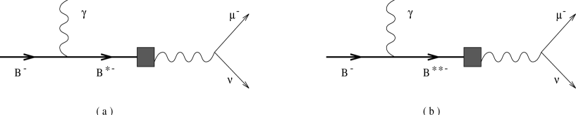
Figure 10: Diagrams dominating the $B^{-}\to\ell^{-}{\bar{\nu}}_{\ell}\gamma$ decay mode in the limit $m_{\ell}\to 0$. $B^{*}$ is the vector meson state, $B^{**}$ is the $1^{+}$ axial vector meson state.

Let us assume, following [144] and [145], that in the pole diagrams the intermediate state is a $J^{P}=1^{-}(B^{*})$ or a positive parity $B^{**}$ meson. The amplitude with intermediate $P(=B^{*},B^{**})$ state is written as follows:

$${\cal M}_{SD}^{(P)}={G_{F}\over\sqrt{2}}V_{ub}{\cal A}(B\to P\gamma){i\over(p-k)^{2}-m^{2}_{P}}<0|{\bar{u}}\gamma^{\mu}(1-\gamma_{5})b|P>{\it l}_{\mu}\hskip 3.0pt,$$ (289)

where $p$ and $k$ are the $B$ and photon momenta respectively, ${\it l}_{\mu}={\bar{\ell}}(p_{\it l})\gamma_{\mu}(1-\gamma_{5})\nu(p_{\nu})$ is the lepton current, ${\cal A}(B\to P\gamma)$ is the amplitude of the process $B\to P\gamma$, and $P$ indicates the pole. When in (289) one takes $P=B^{*}$, the matrix element becomes proportional to $f_{B^{*}}$; therefore, if the contribution of the higher mass resonances is negligible (and we shall see that this is indeed the case), and for light leptons in the final state, the radiative flavour changing $B$ decay can be used to measure the decay constant $f_{B^{*}}$, provided the amplitude ${\cal A}(B^{*}\to B\gamma)$ is known. A direct measurement of the $B^{*}$ width would be extremely difficult (as mentioned in section 6.1, it is less than 1 KeV in all the models); however this amplitude can be indirectly obtained by using the heavy flavour symmetry already employed in section 6.1 to relate the radiative $D^{*}$ and $B^{*}$ decays.

If the partial width $\Gamma(D^{*0}\to D^{0}\gamma)$ is measured (only the branching ratio is available so far, see table 1, then one could extract, from the amplitude

$${\cal A}(D_{a}^{*}(v,\eta)\to D_{a}(v^{\prime})\gamma(q,\epsilon))= i e\left[{e_{c}\over\Lambda_{c}}+{e_{a}\over\Lambda_{a}}\right]$$ (290)

$$M_{D^{*}}\sqrt{M_{D}M_{D^{*}}}\epsilon_{\mu\nu\alpha\beta}\epsilon^{*\mu}\eta^{\nu}v^{\alpha}v^{\prime\beta}\hskip 3.0pt,$$

the mass constant $\Lambda_{a}$ to be used in the formula giving ${\cal A}(B^{*}\to B\gamma)$:

$${\cal A}(B_{a}^{*}(v,\eta)\to B_{a}(v^{\prime})\gamma(q,\epsilon))= i e\left[{e_{b}\over\Lambda_{b}}+{e_{a}\over\Lambda_{a}}\right]$$ (291)

$$M_{B^{*}}\sqrt{M_{B}M_{B^{*}}}\epsilon_{\mu\nu\alpha\beta}\epsilon^{*\mu}\eta^{\nu}v^{\alpha}v^{\prime\beta}\hskip 3.0pt,$$

The expression for the amplitude ${\cal M}_{SD}^{(B^{*})}$ giving the contribution of the $B^{*}$ pole to the decay $B^{-}\to\mu^{-}{\bar{\nu}_{\mu}}\gamma$ is therefore as follows:

$${\cal M}_{SD}^{(B^{*})}={C_{1}f_{B^{*}}\over(v\cdot k+\Delta)}\epsilon_{\mu\sigma\alpha\beta}\l^{\mu}\epsilon^{*\sigma}v^{\alpha}k^{\beta},$$ (292)

where $\Delta=M_{B^{*}}-M_{B}$, and $C_{1}$ is given by:

$$C_{1}={G_{F}\over\sqrt{2}}V_{ub}{M_{B^{*}}\over 2M_{B}}{\sqrt{M_{B^{*}}M_{B}}}\;e\;\Big{[}{e_{b}\over\Lambda_{b}}+{2\over{3\Lambda_{1}}}\Big{]}\hskip 3.0pt.$$ (293)

From (292) one can compute the contribution of the $B^{*}$ pole to $BR(B^{-}\to\mu^{-}{\bar{\nu}}_{\mu}\gamma)$ as a function of the parameter ${\hat{F}}$. Before considering some numerical predictions, let us study the effect of the $B^{**}$ pole, i.e. the positive parity heavy meson having $s_{\ell}=1/2$ (only the axial vector states $1^{+}$ can contribute as poles to the decay; moreover, the state $B_{1}$, having $s_{\ell}=3/2$, has vanishing coupling to the weak current in the limit $m_{b}\to\infty$ [15] (see the discussion after (183); therefore only the state $B_{1}$ (with $s_{\ell}=1/2$) gives a contribution in the same limit.

The contribution of this state is:

$${\cal M}_{SD}^{({\tilde{B}}_{1})}=i{C_{2}f_{B_{1}}\over(v\cdot k+\Delta^{\prime})}(\epsilon\cdot vk_{\mu}-v\cdot k\epsilon_{\mu}){\it l}^{\mu}\hskip 3.0pt$$ (294)

where $\Delta^{\prime}=M_{B_{1}}-M_{B}\simeq 500\,MeV$,

$$<0|{\bar{b}}\gamma_{\mu}\gamma_{5}q|B_{1}(p,\eta)>=f_{B_{1}}M_{B_{1}}\eta_{\mu}~{}~{},$$ (295)

and

$$C_{2}={G_{F}\over\sqrt{2}}V_{ub}{M_{B_{1}}\over 2M_{B}}\sqrt{M_{B}M_{B_{1}}}e\Big{[}{2e_{b}\tau_{1/2}(1)\over M_{B}}+{e_{a}\over\Lambda_{a}^{\prime}}\Big{]}\hskip 3.0pt.$$ (296)

The function $\tau_{1/2}(v\cdot v^{\prime})$ is the universal form factor, analogous to the Isgur-Wise function, that appears in the matrix element of the heavy quark current $J_{\mu}^{h}$ between a positive $s_{\ell}=1/2$ and a negative parity heavy meson state. $\tau_{1/2}(v\cdot v^{\prime})$ has been introduced in [148] and computed in [149] by QCD sum rules, with the result $\tau_{1/2}(1)\simeq 0.24$.

Using this input and the ratio $(f_{B_{1}}/f_{B^{*}})(\Lambda_{a}\Lambda^{\prime}_{a})$ estimated in [145], one obtains

$${\Gamma^{(B_{1})}\over\Gamma^{(B^{*})}}\simeq 0.1\;,$$ (297)

which confirms the previous hypothesis, i.e. that the $B_{1}$ pole represents only a small contribution to the final result.

The results are sensitive to the experimental input $\Gamma(D^{*0}\to D^{0}\gamma)$. For reasonable values of this quantity, which has not been measured yet, one finds for $BR(B^{-}\to\mu^{-}{\bar{\nu}_{\mu}}\gamma)$ a result in the range $10^{-7}-10^{-6}$, i.e. a radiative branching ratio larger than the leptonic $BR(B^{-}\to\mu^{-}\nu)$; the enhancement is obviously still higher if the electron leptonic decay channel is considered, which contributes by a factor of 2. Therefore, in principle, the decay channel $B^{-}\to\mu^{-}{\bar{\nu}}_{\mu}\gamma$ can be used as a way to measure the leptonic $B^{*}$ decay constant.

6.3 Weak radiative decays: $B\to V\gamma$

This section is devoted to the analysis of the exclusive flavour changing radiative $B$ decays with a vector meson in the final state. These channels, at short distances, are described by processes

$$b\to s\gamma$$ (298)

or

$$b\to d\gamma\;,$$ (299)

which are dominated by a penguin diagram with the top as intermediate quark; these decays have been intensively studied in the past [150] and experimental data have been collected both for the inclusive decay [151]:

$$BR(B\to X_{s}\gamma)=(2.32\pm 0.57\pm 0.35)\times 10^{-4}\;,$$ (300)

and for the exclusive decay process

$$B\to K^{*}\gamma$$ (301)

for which the following result has been obtained [152]:

$$BR(B\to K^{*}\gamma)=(4.3^{{\displaystyle+1.1}}_{{\displaystyle-1.0}}\pm 0.6)\times 10^{-5}\;.$$ (302)

The process (301) has been studied within the framework of the heavy quark effective theory [153, 154, 155, 58, 156] (for reviews see [157]), by QCD sum rules [158, 159, 160, 161], [162] or Lattice QCD [163]. In this section we shall review the application of the heavy meson effective chiral lagrangian [164] to the decay process (301) as well as to the other exclusive decay channels

$$B_{s} \to\phi\gamma$$ (303)

$$B \to\rho\gamma$$ (304)

$$B \to\omega\gamma~{}~{}.$$ (305)

Before doing this, let us consider however the simpler approach already considered in section 5.3.1, consisting in the application of the light and heavy flavour symmetries [155].

Let us begin with the $b\to s\gamma$ transition. All the exclusive processes arising from this elementary decay are dominated at the quark level by the short distance $b\to s\gamma$ hamiltonian [150] given by

$$H_{\gamma}=Cm_{b}\bar{s}\sigma^{\mu\nu}(1+\gamma_{5})bF_{\mu\nu}~{}~{}~{}+~{}~{}~{}{\rm h.c.}$$ (306)

(neglecting terms of order $m_{s}/m_{b}$). $F_{\mu\nu}$ is the electromagnetic tensor, $\sigma_{\mu\nu}=\frac{i}{2}[\gamma_{\mu},\gamma_{\nu}]$ and $C$ is given by

$$C=\frac{G_{F}}{\sqrt{2}}\frac{e}{16\pi^{2}}V_{tb}V_{ts}^{*}F_{2}\left(\frac{m_{t}^{2}}{m_{W}^{2}}\right)$$ (307)

where $F_{2}$ is a factor including perturbative QCD corrections, and slightly dependent on the top quark mass. For $m_{t}=175$ GeV, it has the value: $F_{2}=0.63$. Together with the short distance hamiltonian, one should take into account also long distance effects, such as transitions mediated by four quark operators; they will be discussed below.

The short distance hadronic matrix element relevant to the transition $\bar{B}\to K^{*}\gamma$ ($\bar{B}=B^{-}$ or ${\bar{B}}^{0}$) can be expressed as follows:

$$\langle K^{*}(p^{\prime},\epsilon)|\bar{s}\sigma^{\mu\nu}(1+\gamma_{5})b|{\bar{B}}(p)\rangle = i\Big{\{}A(q^{2})\left[p^{\mu}\epsilon^{*\nu}-p^{\nu}\epsilon^{*\mu}-i\epsilon^{\mu\nu\lambda\sigma}p_{\lambda}\epsilon^{*}_{\sigma}\right]$$ (308)

$$+ B(q^{2})\left[p^{\prime\mu}\epsilon^{*\nu}-p^{\prime\nu}\epsilon^{*\mu}-i\epsilon^{\mu\nu\lambda\sigma}p^{\prime}_{\lambda}\epsilon^{*}_{\sigma}\right]$$

$$+ H(q^{2})(\epsilon^{*}\cdot p)\left[p^{\mu}p^{\prime\nu}-p^{\nu}p^{\prime\mu}-i\epsilon^{\mu\nu\lambda\sigma}p_{\lambda}p_{\sigma}^{\prime}\right]\Big{\}}$$

where we have used the property $\frac{i}{2}\epsilon^{\mu\nu\lambda\sigma}\sigma_{\lambda\sigma}\gamma_{5}=-\sigma^{\mu\nu}$.

Now, as first noted in [153], as a consequence of the equations of motion of the heavy quark

$$\frac{1+v\hskip-5.20601pt\lower 0.34723pt\hbox to5.20601pt{\hss\sl/\/\hss}}{2}b=b\;,$$ (309)

in the $b$ rest frame one has

$$\gamma^{0}b=b\;,$$ (310)

which means that

$${\bar{q}}^{a}\sigma_{0i}(1+\gamma_{5})Q=-i{\bar{q}}^{a}\gamma_{i}(1-\gamma_{5})Q\;.$$ (311)

Therefore the form factors (308) can be related to those describing the weak semileptonic transition $B\to K^{*}$ (or $B\to\rho$, using $SU(3)$ symmetry). In computing the width for the decay $B\to K^{*}\gamma$ only the combination of form factors $A+B$ is relevant, whereas $H(q^{2})$ contributes to amplitudes with virtual photons. Using (311), the form factors $A$, $B$ and $H$ are related to the form factors $V$, $A_{1}$ and $A_{2}$ as follows:

$$A(q^{2}) = i\left\{\frac{q^{2}-M_{B}^{2}-m_{K^{*}}^{2}}{M_{B}}\frac{V(q^{2})}{M_{B}+m_{K^{*}}}-\frac{M_{B}+m_{K^{*}}}{M_{B}}A_{1}(q^{2})\right\}$$ (312)

$$B(q^{2}) = i\frac{2M_{B}}{M_{B}+m_{K^{*}}}V(q^{2})$$ (313)

$$H(q^{2}) = \frac{2i}{M_{B}}\left\{\frac{V(q^{2})}{M_{B}+m_{K^{*}}}+\frac{1}{2q^{2}}\frac{q^{2}+M_{B}^{2}-m_{K^{*}}^{2}}{M_{B}+m_{K^{*}}}A_{2}(q^{2})\right\}~{}~{}.$$ (314)

These relations are strictly valid for $q^{2}\approx q^{2}_{max}$. However, following [153, 165, 58] (see however [156] ), one can assume their validity down to the value $q^{2}=0$ which is the kinematical point relevant for decays with a real photon in the final state.

In order to compute $A(0)+B(0)$, one needs the values of the form factors for the transition $B\to K^{*}$; they have been computed by $D\to K^{*}$ semileptonic decays using heavy flavour symmetry (see table 5 of section 5.3.1, neglecting $SU(3)$ flavour breaking). Using the soft pole column result, we have $V^{B\to K^{*}}(0)=0.64$ and $A_{1}^{B\to K^{*}}(0)=0.21$. We observe, however, that, on the basis of the scaling relations given in the previous section, eq. (239), since in this case we assume the same pole behaviour for $V(q^{2})$ and $A_{1}(q^{2})$, the term in $A_{1}$ in eq.(312) is subleading (in $1/m_{Q}$) for any value of $q^{2}>0$ and should be neglected in comparison to the term proportional to $V(q^{2})$, if one works consistently at a given order in the $1/m_{Q}$ expansion. In this way one gets the result:

$$|A(0)+B(0)|=0.53\;.$$ (315)

Following the discussion in section 5.3.1, we may estimate for this result a theoretical uncertainty of at least $\pm 30\%$. We consider now the radiative width, which is given by

$$\Gamma(B\to K^{*}\gamma)=\left(\frac{M_{B}^{2}-m^{2}_{K^{*}}}{2M_{B}}\right)^{3}\frac{2|C|^{2}m_{b}^{2}}{\pi}|A(0)+B(0)|^{2}\;.$$ (316)

One gets

$$BR(B\to K^{*}\gamma)=\left[2.4\times\left(|V_{ts}|/0.039\right)^{2}\right]\times 10^{-5}~{}.$$ (317)

In the previous formula we have used $|V_{tb}|\simeq 1$, $m_{b}=4.7~{}$GeV and $\tau_{B^{+}}\simeq\tau_{B^{0}}\simeq\tau_{B_{s}}\simeq 1.55~{}ps$. The result based on (315) agrees within the errors with the experimental finding (302). It should be noted that eq.(317) does not include long distance effects due the $c\bar{c}$ quark loop [166] that raise the branching ratio by $\approx 20\%$, thus improving the agreement; we shall discuss them in more detail below. A similar analysis, with obvious changes, applies to the decay $B_{s}\to\phi\gamma$ and one obtains

$$BR(B_{s}\to\phi\gamma)\approx BR(B\to K^{*}\gamma)~{},$$ (318)

due to approximate $SU(3)$ light flavour symmetry.

Now we discuss how the $b\to s\gamma$ exclusive decays can be described by the effective chiral lagrangian approach.

At the lowest order in the derivatives of the pseudoscalar field, the weak tensor current between light pseudoscalar and negative parity heavy mesons is as follows:

$$L_{\mu\nu}^{a}=i\frac{{\hat{F}}}{2}<\sigma_{\mu\nu}(1+\gamma_{5})H_{b}\xi^{\dagger}_{ba}>~{},$$ (319)

and it has the same transformation properties of the quark current ${\bar{q}}^{a}\sigma^{\mu\nu}(1+\gamma_{5})Q$. Together with (319) we also consider the weak effective current (177) corresponding to the quark $V-A$ current ${\bar{q}}^{a}\gamma^{\mu}(1-\gamma_{5})Q$:

$$L_{\mu}^{a}=i\frac{{\hat{F}}}{2}\langle\gamma_{\mu}(1-\gamma_{5})H_{b}\xi^{\dagger}_{ba}\rangle~{}~{}.$$ (320)

We put the same coefficient $i{\hat{F}}/2$ in both (319) and (320) because, due to (311), the relation

$$L_{0i}=-iL_{i}$$ (321)

must be satisfied.

We also introduce the weak tensor current containing the light vector meson $\rho^{\alpha}$ and reproducing the bilinear ${\bar{q}}^{a}\sigma^{\mu\nu}(1+\gamma_{5})Q$

$$L_{1a}^{\mu\nu}=i\alpha_{1}\left\{g^{\mu\alpha}g^{\nu\beta}-\frac{i}{2}\epsilon^{\mu\nu\alpha\beta}\right\}\langle\gamma_{5}H_{b}\left[\gamma_{\alpha}(\rho_{\beta}-{\cal V}_{\beta})_{bc}-\gamma_{\beta}(\rho_{\alpha}-{\cal V}_{\alpha})_{bc}\right]\xi^{\dagger}_{ca}\rangle~{}~{}.$$ (322)

$L_{1a}^{\mu\nu}$ is related to the vector current $L_{1a}^{\mu}$, eq. (182), introduced to describe at the meson level the quark current operator ${\bar{q}}^{a}\gamma^{\mu}(1-\gamma_{5})Q$ taken between light vector particles and heavy mesons:

$$L_{1a}^{\mu}=\alpha_{1}\langle\gamma_{5}H_{b}(\rho^{\mu}-{\cal V}^{\mu})_{bc}\xi^{\dagger}_{ca}\rangle$$ (323)

(we keep only the leading term in $1/m_{Q}$). We notice that in order to construct the tensor current we have imposed (321).

To compute $B\to K^{*}\gamma$ we consider a pole diagram having as intermediate state between the current and the $BK^{*}$ system either a $1^{+}$ or a $1^{-}$ heavy meson; moreover we add a direct term. The effective lagrangian and the effective tensor currents can reliably describe the process only for large values of $q^{2}$, i.e. $q^{2}\approx q^{2}_{max}=(M_{B}-m_{K^{*}})^{2}$. This is a general feature of the chiral lagrangian approach. Again, in order to extend our results to small values of $q^{2}$, we shall assume a polar dependence in $q^{2}$ (with pole mass suggested by dispersion relations). By following a procedure similar to section 5.3.2, we obtain the results of table 10 that are valid for any $q^{2}$ and in the limit $m_{Q}\to\infty$. We notice that in writing the various contributions in table 10 we have left the dependence of $p\cdot p^{\prime}$ on $q^{2}$, $p\cdot p^{\prime}=(M_{B}^{2}+m_{K^{*}}^{2}-q^{2})/2$, in the term arising from the $1^{-}$ pole and we have assumed that the direct term has a pole dependence with mass given by the $1^{+}$ pole. These choices can be justified as follows. The results in table 10 satisfy, for $q^{2}\approx q^{2}_{max}$, the relations (312 - 314) between form factors of vector and tensor currents. Eqs. (312) and (313) coincide with the relations found in ref. [153]; as for (314), the result of [153]:

$$H(q^{2})=\frac{2i}{M_{B}}\Big{\{}\frac{V(q^{2})}{M_{B}+m_{K^{*}}} + \frac{1}{2q^{2}}\Big{(}\frac{q^{2}+M_{B}^{2}-m_{K^{*}}^{2}}{M_{B}+m_{K^{*}}}A_{2}(q^{2})$$ (324)

$$+ 2m_{K^{*}}A_{0}(q^{2})-(M_{B}+m_{K^{*}})A_{1}(q^{2})\Big{)}\Big{\}}$$

differs from (313) for terms that are subleading in the limit $m_{Q}\to\infty$ and can be neglected.

Table 10: Terms contributing to the various form factors of the transition $B\to K^{*}\gamma$. $m_{P}$ is the pole mass ($m_{P}=5.9~{}$GeV for the direct and $1^{+}$ term; and $5.43~{}$GeV for the $1^{-}$ contribution). $p\cdot p^{\prime}=(M_{B}^{2}+m_{K^{*}}^{2}-q^{2})/2$.

${\rm Form~{}Factor}$	${\rm Direct}$	$1^{-}$	$1^{+}$
$A(q^{2})$	$\displaystyle{\frac{i\sqrt{2}g_{V}\alpha_{1}}{\sqrt{M_{B}}}\frac{q^{2}_{max}-m_{P}^{2}}{q^{2}-m_{P}^{2}}}$	$\displaystyle{\frac{i2\sqrt{2}{\hat{F}}\lambda g_{V}(p\cdot p^{\prime})}{(m_{P}^{2}-q^{2})\sqrt{M_{B}}}}$	$\displaystyle{\frac{-i\sqrt{2M_{B}}{\hat{F}}^{+}g_{V}(\zeta-2\mu m_{K^{*}})}{m_{P}^{2}-q^{2}}}$
$B(q^{2})$	0	$\displaystyle{\frac{-i2\sqrt{2}{\hat{F}}\lambda g_{V}M_{B}^{3/2}}{m_{P}^{2}-q^{2}}}$	0
$H(q^{2})$	0	$\displaystyle{\frac{-i2\sqrt{2}{\hat{F}}\lambda g_{V}}{(m_{P}^{2}-q^{2})\sqrt{M_{B}}}}$	$\displaystyle{\frac{-i2\sqrt{2M_{B}}{\hat{F}}^{+}g_{V}\mu}{(m_{P}^{2}-q^{2})M_{B}}}$

Following [153] and [165] and our previous discussion, we assume that the results (312 - 314) hold also for small values of $q^{2}$, which justifies the above mentioned choices in table 10.

Before computing the entries of table 10 let us observe that the results in the columns ”Direct” and $1^{+}$ are subleading as compared to those in the column $1^{-}$. In other terms

$$\frac{(A+B)_{Direct+1^{+}}}{(A+B)_{1^{-}}}=O\left(\frac{1}{m_{b}}\right)$$ (325)

for any value of (positive) $q^{2}$. Therefore, consistently with the neglect of the $O({1}/{m_{b}})$ contributions, we do not keep them, which means that only the term arising from the exchange of the $1^{-}$ particle is taken into account. In this way one obtains:

$$A(q^{2})+B(q^{2})=-i\sqrt{\frac{2}{M_{B}}}\frac{{\hat{F}}\lambda g_{V}}{M^{2}_{B^{*}_{s}}}(q^{2}+M_{B}-m^{2}_{K^{*}})\;,$$ (326)

which gives, for ${\hat{F}}=0.30~{}{\rm GeV}^{3/2}$, $g_{V}=5.8$ (see eq. (65)) and $\lambda=-0.41~{}{\rm GeV}^{-1}$ (eq.(285)), the result:

$$|A(0)+B(0)|=0.41,$$ (327)

and, therefore, $BR(B\to K^{\star}\gamma)=\left[1.4\times\left(V_{ts}/0.039\right)^{2}\right]\times 10^{-5}$. A similar analysis, with obvious changes, applies to the decay $B_{s}\to\phi\gamma$. In this case one obtains $|A(0)+B(0)|=0.42$ and $BR(B_{s}\to\phi\gamma)=\left[1.6\times\left(V_{ts}/0.039\right)^{2}\right]\times 10^{-5}$. In table 11 we compare the analyses based on the scaling approach and on effective chiral lagrangian to the results of QCD sum rule calculations [159, 161]; other QCD sum rules analyses [160, 162] agree with [159] and [161]. We note that the results based on the use of the heavy flavour symmetry (first and second row in the table) are generally smaller than the QCD sum rules outcome.

Table 11: Theoretical values of the $B\to K^{*}\gamma$ coupling $|A(0)+B(0)|$ in different approaches: soft pole, chiral lagrangian, QCD sum rules calculations based on the evaluation of three point function and light cone sum rules respectively.

Model		$|A(0)+B(0)|$
soft pole (sec.5.3.1)		0.53
$\chi$-lagrangian eq.(326)		$0.41$
QCD sum rules [159]		$0.70\pm 0.10$
QCD sum rules [161]		$0.64\pm 0.10$

Also lattice QCD [163] has been used to compute the transition $B\to K^{*}\gamma$; however in this approach the couplings for this decay are computed near the zero recoil point and for a heavy quark mass smaller than its physical value. Therefore a double extrapolation is needed to compute them and it is hard to compare these outcomes, that should be considered as still preliminary, with QCD sum rules or chiral lagrangian approaches. As for the comparison with the experimental data, as we have already mentioned, one should take into account also the so called long distance (LD) effects, that we now discuss.

Let us begin with the decays (304) and (305), where these effects are larger. The decays $B\to\rho\gamma$ and $B\to\omega\gamma$ take contributions both from the short distance and the long distance mechanisms. The former is generated by a hamiltonian similar to eq. (306), with obvious modifications ($s\to d$ and $V_{ts}\to V_{td}$). For it an analysis similar to the one employed in $B\to K^{*}\gamma$ applies, but it is obvious that this contribution is Cabibbo suppressed as compared to $B\to K^{*}\gamma$, which can explain why the $\rho\gamma$ final state is more difficult to measure (and indeed it has not been observed yet). Because of the smallness of the short distance contribution, LD effects are more important in these decays than in $B\to K^{*}\gamma$ or $B_{s}\to\phi\gamma$ . For $B^{+}\to\rho^{+}\gamma$ decay, their contribution has been estimated by QCD sum rules [167, 168]. The ratio of the long distance to the short distance amplitudes, as expressed by

$$\frac{A_{LD}(B^{+}\to\rho^{+}\gamma)}{A_{SD}(B^{+}\to\rho^{+}\gamma)}=R\left|\frac{V_{ub}V_{ud}}{V_{td}V_{tb}}\right|~{},$$ (328)

is estimated to be [167]: $R=-0.30\pm 0.07$, i.e. a significant contribution. LD effects mainly contribute to the weak annihilation diagrams and are therefore relevant for $B^{+}\to\rho^{+}\gamma$, but less important for $B\to\rho,\omega\gamma$. For $B\to K^{*}\gamma$ one does not expect significant contributions from the weak annihilation diagrams because of the CKM suppression (CKM non suppressed terms can contribute by non factorizable diagrams, whose role, however, has been found to be very small [169]). Other LD contributions come from the four quark operator $O_{2}\approx\bar{c}_{L}\gamma_{\mu}c_{L}\bar{s}_{L}\gamma^{\mu}b_{L}$ (or $O_{2}\approx\bar{c}_{L}\gamma_{\mu}c_{L}\bar{d}_{L}\gamma^{\mu}b_{L}$ for $B\to\rho\gamma$). It contributes via a charm quark loop (the up quark loop gives a negligible contribution), with the photon emitted by the charm quark line, and adds about $20\%$ to the $B\to K^{*}\gamma$ width [166]; by duality this contribution may be seen as the result of a mechanism where $K^{*}J/\psi$ are produced via $O_{2}$, with photon conversion of $J/\psi$ [170, 171, 172, 173]; even though less reliable, the estimates of LD contributions based on this mechanism seem to agree [170] with the result of the charm loop calculation. Similar results hold also for the $B\ \to\rho\gamma$ decays [166, 174, 175].

6.4 Weak radiative decays: $B\to Ke^{+}e^{-},\;B\to K^{*}e^{+}e^{-}$

In this section we discuss the decays

$$B \to Ke^{+}e^{-}$$ (329)

$$B \to K^{*}e^{+}e^{-}~{}.$$ (330)

They occur dominantly via a quark process $b\to s\gamma^{*}\to se^{+}e^{-}$ ($\gamma^{*}=$ virtual photon). In the effective lagrangian for $b\to se^{+}e^{-}$ we have to include also the already mentioned long-distance contributions; they produce $\psi-\gamma$ or $\psi^{\prime}-\gamma$ conversion, and are seen as peaks in the lepton pair invariant mass distribution. The effective lagrangian has been derived in [176], [177] and we shall not report it here for the sake of simplicity.

Let us begin with $B\to Ke^{+}e^{-}$. The transition $B\to K\gamma$ can occur only by virtual photons and is described at short distance by the hamiltonian (306) and, therefore, by the hadronic matrix element

$$\langle K(p^{\prime})|\bar{s}\sigma^{\mu\nu}(1+\gamma_{5})b|{\bar{B}}(p)\rangle=iS(q^{2})\left[p^{\mu}p^{\prime\nu}-p^{\nu}p^{\prime\mu}-i\epsilon^{\mu\nu\lambda\sigma}p_{\lambda}p_{\sigma}^{\prime}\right]~{}.$$ (331)

The form factor $S(q^{2})$ can be related, by using the heavy quark equation of motion and eq. (311), [153], to the form factors $F_{1}(q^{2})$ and $F_{0}(q^{2})$ for the weak transition $B\to K$ via the vector current. In this way one finds [153]:

$$S(q^{2})=\frac{1}{M_{B}}\left[-F_{1}(q^{2})+\frac{m^{2}_{K}-M^{2}_{B}}{q^{2}}\left(F_{1}(q^{2})-F_{0}(q^{2})\right)\right]~{}.$$ (332)

Let us now consider the calculation of the transition $B\to K$ by tensor current in the effective chiral lagrangian approach [164]. At the tree level the relevant hamiltonian is given by (319) together with the strong hamiltonian $BB^{*}\pi$ of eq. (38). The short distance diagrams are similar to those of $B\to K^{*}\gamma$, that we have described in some detail in the preceeding section. In this case, however, at tree level, there is no direct coupling, and the only surviving term, in the limit $m_{b}\to\infty$, and for $q^{2}\approx q^{2}_{max}$, is the pole contribution.

Assuming a $q^{2}$ dependence of a simple pole, with $M_{P}=M_{B^{*}_{s}}$ (as discussed before, this seems a reasonable assumption for $F_{1}$ related form factors), one gets the result:

$$S(q^{2})=\frac{S(0)}{1-q^{2}/M^{2}_{B_{s}^{*}}}$$ (333)

with

$$S(0)=\frac{{\hat{F}}g}{f_{\pi}M^{2}_{B^{*}_{s}}\sqrt{M_{B}}}(M_{B^{*}_{s}}+M_{B}-m_{K})~{}~{}.$$ (334)

When expressed in terms of the form factors of the $B\to K$ transition by vector current, this result is:

$$S(q^{2})=-\frac{2F_{1}(q^{2})}{M_{B}}$$ (335)

which coincides with the Isgur and Wise relation (332) only at $q^{2}\approx q^{2}_{max}$ and $M_{B}\to\infty$, namely in the range of validity of the effective hamiltonian. Exactly as in the case of $B\to K^{*}\gamma$ transition, we find that some form factors (in this case $F_{0}$) are subleading when $m_{Q}\to\infty$, which is expected because the $0^{+}$ state, contributing to $F_{0}$, cannot couple to the antisymmetric tensor current $\bar{s}\sigma_{\mu\nu}(1+\gamma_{5})b$.

The numerical result of this analysis is as follows: using $g\simeq 0.38$ and ${\hat{F}}=0.30$ GeV^3/2, one obtains

$$S(0)\simeq-0.13~{}{\rm GeV}^{-1}~{}~{}.$$ (336)

This result already contains some SU(3) corrections, namely in the meson masses, but the bulk of the chiral corrections should come from loops containing pseudoscalar bosons ($\pi$, $K$ and $\eta$). They have been computed in [68]. Three classes of corrections are found. First one has correction to the pole amplitude (334); second there are corrections to the direct term (called point contribution in [68]); last there is the renormalization of the $B$ meson wavefunction. Taking into account only the nonanalytic corrections that arise from the loop diagrams, and having no uncertainty related to unknown analytic higher order terms in the phenomenological lagrangian, one finds [68] a correction of $-51\%$ to the dominant pole contribution (the correction to the direct term is much smaller).

This analysis, as stressed in [68], is not conclusive, since the analytic corrections could be significant; nevertheless it is interesting to observe that, with the nonanalytic correction alone, the outcome of the effective chiral lagrangian becomes $S(0)\approx-0.06$ GeV^-1, which is compatible with the result of a QCD sum rules analysis based on three point functions [178]: $S(0)=-0.05\pm 0.01$ GeV^-1 .

The results we have reported, together with the long distance contributions [176, 177], can be used to obtain the distribution $d\Gamma(B\to Ke^{+}e^{-})/dq^{2}$ in the invariant mass squared of the lepton pair $Q^{2}$. This distribution is dominated by the contribution of the resonances $J/\psi$ and $\psi^{\prime}$; however, as discussed for instance in [178], for $Q^{2}$ far from the resonance masses, one could still obtain from the data, when available, useful information on the short distance dynamics.

The same analysis can be performed for $d\Gamma(B\to K^{*}e^{+}e^{-})/dQ^{2}$. The long distance contribution can be evaluated starting from experimental data on the nonleptonic decay modes $B\to K^{\star}J/\psi$ and $B\to K^{\star}\psi^{\prime}$. For the short distance part one needs the form factors $A(q^{2})$, $B(q^{2})$ and $H(q^{2})$ we have defined in eq. (308). In the effective lagrangian approach one finds, from table 10

$$A(q^{2}) = \frac{i\sqrt{2}{\hat{F}}\lambda g_{V}(m^{2}_{B}+m^{2}_{K^{*}}-q^{2})}{(M_{B_{s}^{*}}^{2}-q^{2})\sqrt{M_{B}}}$$ (337)

$$B(q^{2}) = \frac{-i2\sqrt{2}{\hat{F}}\lambda g_{V}M_{B}^{3/2}}{M_{B_{s}^{*}}^{2}-q^{2}}$$ (338)

$$H(q^{2}) = \frac{-i2\sqrt{2}g_{V}}{\sqrt{M_{B}}}\left[\frac{{\hat{F}}\lambda}{M_{B_{s}^{*}}^{2}-q^{2}}+\frac{{\hat{F}}^{+}\mu}{M_{B_{s}^{**}}-q^{2}}\right]$$ (339)

where $B_{s}^{**}$ is the $1^{+}$ $\bar{s}b$ resonance. $A(0)$ and $B(0)$ have been discussed in section 6.3; as for $H(0)$, using (285) and the result of section 5.3.2 (obtained with $r=0.5$): $\mu=-0.10$ GeV^-1, together with ${\hat{F}}=0.30$ GeV^3/2 and ${\hat{F}}^{+}=0.46$ GeV^3/2, eq. (181), one gets:

$$|H(0)|=0.04~{}{\rm GeV}^{-2}$$ (340)

to be compared with the QCD sum rule result [178] $|H(0)|\approx 0.10~{}{\rm GeV}^{-2}$. Analogously to the $A(0)+B(0)$ case (see table 11), we see that the chiral lagrangian approach at tree level gives significantly smaller results than QCD sum rules, which might indicate either a relevant $1/m_{Q}$ correction or, most probably, a relevant contribution from chiral loop, similarly to the case of $S(0)$ discussed above.

The distribution in the invariant mass of the lepton pair is largely dominated by the long distance contributions [179, 172], exactly as for the $Ke^{+}e^{-}$ final state; nevertheless an accurate measurement of the lepton pair spectrum below $c\bar{c}$ resonances would display the effects of the short distance hamiltonian. This measurement would therefore complement the analysis of the $B\to K^{*}\gamma$ decay process, providing further information on the fundamental parameters appearing in the short distance hamiltonian as well as on the validity of the effective lagrangian approach.

7 Symmetries for heavy quarkonium states

Quarkonium, a heavy quark-antiquark bound state, is one of the most interesting systems for the study of quantum chromodynamics (QCD). The physical idea is that quarks with mass larger than the QCD scale $\Lambda_{QCD}$ would form bound states resembling positronium [180]. Many properties of quarkonium can be predicted by the use of non-relativistic potential models. The overall description one obtains in this way for the charmonium and bottomonium spectroscopies is quite satisfactory provided corrections originated by leading relativistic terms are included and the possible multichannel structure of the phenomenon is taken into account for certain expected effects [180].

The heavy quark and anti-quark are bound in these models by an instantaneous potential, meaning that gluons have typical interaction times much shorter than the time scale associated with the motion of the heavy quarks. We indicate with $k$ the relative momentum and with $v_{r}=k/m_{Q}$ the relative velocity between the two heavy quarks of mass $m_{Q}$. It is interesting to examine the dependence of these quantities on the quark mass.

For instance, Buchmüller and Tye [181] have studied a QCD-motivated potential reproducing the behaviour $1/r$ for small $r$, and behaving as $r$ at large distances (this model is similar to the model in [55]). Analogous results can be obtained using other models, such as Quigg and Rosner [182] or Grant and Rosner [183], indicating that, by increasing the quark mass, the kinetic energy and the residual momentum increase, whereas the relative velocity decreases. Going further up with the mass $m_{Q}$, the heavy quarks separation becomes smaller, and eventually the Coulomb term of the potential energy, proportional to $\alpha_{s}/r$ will dominate ($\alpha_{s}$ is the strong coupling constant evaluated at the momentum scale $1/r$). Taking $r$ of the order of the size of the bound state $1/(m_{Q}v_{r})$ in the potential energy and equating its average value to the kinetic term we get $<v_{r}>\approx\alpha_{s}$, with $\alpha_{s}$ evaluated at the momentum scale $m_{Q}v_{r}$, going to zero in the limit $m_{Q}\to\infty$. We notice that in such a coulombic regime the relative velocity decreases logarithmically.

Concerning the spin symmetry, the coupling of the gluon to the spin of the heavy quark is expected to be of the order $p_{g}/m_{Q}$, with the gluon momentum $p_{g}\approx k$. Therefore the quantity $k/m_{Q}=v_{r}$ gives information on the degree of spin decoupling, and strictly in the limit $m_{Q}\to\infty$ one has an exact spin symmetry.

The heavy quark flavour symmetry, on the contrary, is badly broken in quarkonium systems. In general the gluon radiation exchanged between static quarks gives rise to infrared divergences. In a bound state, potential and kinetic energy play a delicate balance against each other [184]. The regularization of the infrared divergences then implies a large breaking of flavour symmetry because of the explicit appearance of the heavy quark mass in the kinetic energy.

For charmonium, potential models give $<v_{r}>\approx 0.5$, for bottomonium $<v_{r}>\approx 0.25$; one expects corrections, even important, to the “leading order” velocity and spin symmetry description, especially for charmonium.

7.1 Non-relativistic QCD description

An effective approach to quarkonium is given by the non-relativistic heavy quark QCD description, which provides a general factorization formula for annihilation decay rates of heavy quarkonium [185]. It consists in exploiting the fact that in quarkonium the heavy quark moves with a small relative velocity and nonrelativistic quantum chromodynamics (NRQCD) is a good approximation. The lowest order dynamics is given by the Schrödinger equation for the heavy quarks. The resulting effective theory [186] consists in fact of a nonrelativistic Schrödinger field theory for the heavy quarks coupled to the relativistic theory for gluons and light quarks. Relativistic corrections can be included systematically into this picture at any given order in the heavy quark velocity $v$.

In this framework the scales entering the problem are written in terms of the heavy quark velocity $v$ and mass $m_{Q}$. As shown before, the typical velocity of the heavy quark decreases as the mass increases. When $m_{Q}$ is sufficiently large, the heavy quark and antiquark are non-relativistic ($v<<1$) and the scales $m_{Q}$, $m_{Q}v$ (typical three-momentum of the heavy quark in the meson rest frame), and $m_{Q}v^{2}$ (typical kinetic energy) are well separated:

$$\Lambda^{2}_{QCD}\ll(m_{Q}v^{2})^{2}\ll(m_{Q}v)^{2}\ll m_{Q}^{2}$$ (341)

In NRQCD the effects at the scale $m_{Q}$ are taken into account through the coupling constants of 4-fermion operators, while the effects of the lower momentum scales $m_{Q}v$, $m_{Q}v^{2}$, and $\Lambda_{QCD}$ are included into matrix elements organized in terms of their dependence on $v^{2}$. The lagrangian is obtained from QCD by introducing an ultraviolet cut-off of the order $m_{Q}$, which excludes relativistic heavy quarks from the theory. It also excludes light quarks and gluons with momenta of order $m_{Q}$. Then the heavy-quark and heavy-antiquark degrees of freedom are decoupled by a Foldy-Wouthuysen transformation. The full NRQCD lagrangian consists of the part describing the heavy quarks and anti-quarks in terms of a non-relativistic Schrödinger theory with separate two-component fields for the quarks and anti-quarks ${\cal{L}}_{heavy}$, plus a fully relativistic part for the light quarks and gluons ${\cal{L}}_{light}$, plus a correction term $\delta{\cal{L}}$ reproducing the relativistic effects of full QCD in terms of new local interactions:

$${\cal{L}}_{NRQCD}={\cal{L}}_{light}+{\cal{L}}_{heavy}+\delta{\cal{L}}$$ (342)

with

$${\cal{L}}_{heavy}=\psi^{{\dagger}}\left(iD_{o}+\frac{{\bf D}}{2m_{Q}}\right)\psi+\chi^{{\dagger}}\left(iD_{0}+\frac{{\bf D}}{2m_{Q}}\right)\chi~{}~{},$$ (343)

where $\psi$ and $\chi$ are the two component fields for quarks and anti-quarks and $D_{0}$ and ${\bf D}$ are the time and space components of the covariant derivative. The term $\delta{\cal{L}}$ contains all possible gauge invariant counterterms, whose coefficients must be matched with QCD in order to avoid ultraviolet divergences in the calculation of long distance quantities and to reproduce the results of full QCD. In principle the NRQCD lagrangian consists of infinitely many terms. However they can be classified in powers of the heavy quark velocity $v$ and their relative importance can be established.

The annihilation of quarkonium can be reproduced in this framework only indirectly, through its effects on $Q\bar{Q}$ scattering amplitudes. At long distance, these amplitudes can be described adding to the lagrangian four fermion operators that annihilate and create a heavy quark-antiquark pair. Due to the optical theorem the imaginary parts of the coefficients of the four fermion operators are related to the annihilation of heavy quarkonium. It should be noted that the annihilation decay rates for heavy quarkonium are small perturbations of the energy levels. In this approach the contributions to annihilation widths from the dimension-6 four fermion operators contain extra suppression factors, due to the coefficients of the operators. The widths are of order $\alpha_{s}^{2}(m_{Q})v$ or smaller, while the splitting between radial excitations is of order $m_{Q}v^{2}$.

7.2 Heavy quarkonium effective theory

Quarkonium, in the heavy quarkonium effective theory [187, 188, 189] is described as a bound state in the particle-antiparticle sector of the HQET [2, 3, 4]. In quarkonium systems the internal motion of the heavy quarks cannot be neglected due to the delicate balance between the potential and kinetic energy in the bound state. This suggests to go beyond the static limit to describe quarkonia states. One must therefore keep the kinetic energy operator even when working at the lowest order. The kinetic energy operator is spin symmetric, but it includes a factor of $1/m_{Q}$. Therefore heavy flavour symmetry is lost while spin symmetry is still present. The leading order lagrangian is [188]:

$${\cal L}_{0}={\bar{h}}_{v}^{(+)}(ivD)h_{v}^{(+)}+{\bar{h}}_{v}^{(+)}\frac{(iD)^{2}}{2m_{Q}}h_{v}^{(+)}-{\bar{h}}_{w}^{(-)}(iwD)h_{w}^{(-)}+{\bar{h}}_{w}^{(-)}\frac{(iD)^{2}}{2m_{Q}}h_{w}^{(-)}~{}~{},$$ (344)

where as usual a sum over heavy quark velocities is understood. The heavy field is obtained from the field $Q$ of QCD by removing the dominant part of the heavy quark momentum:

$$Q=\exp(-im_{Q}vx)\left(1+\frac{1+v\hskip-5.20601pt\lower 0.34723pt\hbox to5.20601pt{\hss\sl/\/\hss}}{2}\frac{D\hskip-8.55695pt\lower-0.91666pt\hbox to8.55695pt{\hss\sl/\/\hss}}{2m_{Q}}+{\cal O}(1/m_{Q}^{2})\right)h_{v}^{(+)}(x)$$ (345)

and $h_{v}^{(+)}$ describes a quark with velocity $v$. In a similar way $h_{w}^{(-)}$ describes an anti-quark moving with velocity $w$. The lagrangian in (344) is the starting point of an effective lagrangian description of heavy quarkonium decays. The two velocities of the heavy quarks differ only by a quantity of the order of $\Lambda_{QCD}/m_{Q}$ so that it is convenient to work in the limit in which the two heavy quark velocities become equal. This limit can be taken consistently starting from the effective lagrangian (344). In any case a mass dependence in the lowest order dynamics is unavoidable so that heavy flavour symmetry is destroyed. In this picture spin symmetry, as we anticipated, still holds since the kinetic energy operator is spin symmetric.

As to relativistic corrections (proportional to the relative velocity of the heavy quarks) and non-perturbative corrections, they turn out to have the same origin in this approach, namely they come from higher order terms of the $1/m_{Q}$ expansion. Short and long distance contributions for the inclusive annihilation decays are separated by means of the operator product expansion. The distance scale is given by the Compton wavelength of the heavy quark. The annihilation rates are written in an expansion in $({\tilde{\Lambda}}/m_{Q})$ where $\tilde{\Lambda}$ is the inverse Bohr radius of the system. The coefficients of this expansion can be calculated perturbatively.

This approach is similar to the one of non-relativistic QCD and in fact in that case the lowest order dynamics is basically the one obtained by adding the kinetic energy operator to the static HQET part. The two approaches are not completely equivalent though: for example if we consider two operators like the gluon field strength $[iD,iD]$ and $(iD)^{2}$, they have the same dimension, but they are not equivalent if an expansion in relative velocity $v/c$ is considered, as in the case of NRQCD (for a detailed comparison of the two approaches see [189]). In any event if the same set of assumptions is applied in the two cases, both the approaches yield the same results up to the order $({\tilde{\Lambda}}/m_{Q})^{2}$.

7.3 Heavy-meson effective theory

This approach consists in constructing a heavy meson multiplet field and writing a lagrangian including the exact and approximate symmetries of the problem [190]. The procedure is analogous to the one introduced in the preceeding chapters of this review treating of heavy-light mesons. Symmetry breaking terms can be easily added to the formalism as we shall show in the following. The velocity description and spin symmetry are still useful, but flavour symmetry is broken. As in the single heavy quark case [10, 11, 12], an effective lagrangian describing the low-momentum interactions of heavy quarkonia with light mesons can be written down. The heavy quarkonium multiplets are described by a simple trace formalism [6], which can be also applied to the description of the $B_{c}$ system.

7.3.1 Heavy quarkonium states

A heavy quark-antiquark bound state, characterized by the radial number $m$, the orbital angular momentum $l$, the spin $s$, and the total angular momentum $J$, is denoted by:

$$m\,^{2s+1}l_{J}$$ (346)

Parity $P$ and charge conjugation $C$, which determine selection rules for electromagnetic and hadronic transitions, are given by:

$$P=(-1)^{l+1}$$ (347)

$$C=(-1)^{l+s}$$ (348)

and are exactly conserved quantum numbers for quarkonium, together with $J$. If spin dependent interactions are neglected, it is natural to describe the spin singlet $m\,^{1}l_{J}$ and the spin triplet $m\,^{3}l_{J}$ by means of a single multiplet $J(m,l)$. For the case $l=0$, when the triplet $s=1$ collapses into a single state with total angular momentum $J=1$, this is readily realized:

$$J=\frac{(1+v\hskip-5.20601pt\lower 0.34723pt\hbox to5.20601pt{\hss\sl/\/\hss})}{2}[H_{\mu}\gamma^{\mu}-\eta\gamma_{5}]\frac{(1-v\hskip-5.20601pt\lower 0.34723pt\hbox to5.20601pt{\hss\sl/\/\hss})}{2}~{}~{}.$$ (349)

Here $v^{\mu}$ denotes the four velocity associated to the multiplet $J$; $H_{\mu}$ and $\eta$ are the spin 1 and spin 0 components respectively; the radial quantum number has been omitted. The expressions for the general wave $J^{\mu_{1}\ldots\mu_{l}}$ are given in the appendix C. In the sequel $K_{l}^{\mu_{1}\ldots\mu_{l}}$ represents the spin singlet component $~{}^{1}l_{J}$, $H_{l+1,l,l-1}^{\mu_{1}\ldots\mu_{l+1}}$ the spin triplet $~{}^{3}l_{J}$ in the wave $J^{\mu_{1}\ldots\mu_{l}}$.

From eqs. (347) and (348) one has the following transformation properties of $H_{l}$ and $K_{l}$ under parity and charge conjugation:

$$H_{l+1}^{\mu_{1}\ldots\mu_{l+1}} \stackrel{{\scriptstyle P}}{{\rightarrow}} H^{l+1}_{\mu_{1}\ldots\mu_{l+1}}$$

$$H_{l}^{\mu_{1}\ldots\mu_{l}} \stackrel{{\scriptstyle P}}{{\rightarrow}} -H^{l}_{\mu_{1}\ldots\mu_{l}}$$

$$H_{l-1}^{\mu_{1}\ldots\mu_{l-1}} \stackrel{{\scriptstyle P}}{{\rightarrow}} H^{l-1}_{\mu_{1}\ldots\mu_{l-1}}$$

$$K_{l}^{\mu_{1}\ldots\mu_{l}} \stackrel{{\scriptstyle P}}{{\rightarrow}} -K^{l}_{\mu_{1}\ldots\mu_{l}}$$ (350)

$$H_{l+1,l,l-1}^{\mu_{1}\ldots\mu_{l+1,l,l-1}} \stackrel{{\scriptstyle C}}{{\rightarrow}} (-1)^{l+1}H_{l+1,l,l-1}^{\mu_{1}\ldots\mu_{l+1,l,l-1}}$$

$$K_{l}^{\mu_{1}\ldots\mu_{l}} \stackrel{{\scriptstyle C}}{{\rightarrow}} (-1)^{l}K_{l}^{\mu_{1}\ldots\mu_{l}}$$ (351)

As one can easily verify, the previous transformations laws are reproduced by assuming that the multiplet $J^{\mu_{1}\ldots\mu_{l}}$ transforms as follows:

$$J^{\mu_{1}\ldots\mu_{l}} \stackrel{{\scriptstyle P}}{{\rightarrow}} \gamma^{0}J_{\mu_{1}\ldots\mu_{l}}\gamma^{0}$$

$$v^{\mu} \stackrel{{\scriptstyle P}}{{\rightarrow}} v_{\mu}$$ (352)

$$J^{\mu_{1}\ldots\mu_{l}} \stackrel{{\scriptstyle C}}{{\rightarrow}} (-1)^{l+1}CJ^{\mu_{1}\ldots\mu_{l}T}C$$ (353)

where $C=i\gamma^{2}\gamma^{0}$ is the usual charge conjugation matrix.

Under heavy quark spin transformation one has

$$J^{\mu_{1}\ldots\mu_{l}}\rightarrow SJ^{\mu_{1}\ldots\mu_{l}}S^{\prime\dagger}$$ (354)

with $S,\,S^{\prime}\in SU(2)$ and $[S,v\hskip-5.20601pt\lower 0.34723pt\hbox to5.20601pt{\hss\sl/\/\hss}]=[S^{\prime},v\hskip-5.20601pt\lower 0.34723pt\hbox to5.20601pt{\hss\sl/\/\hss}]=0$. As long as one can neglect spin dependent effects, one will require invariance of the allowed interaction terms under the transformation (354).

Finally under a Lorentz transformation $\Lambda$ we have:

$$J^{\mu_{1}\ldots\mu_{l}}\rightarrow\Lambda^{\mu_{1}}_{~{}\nu_{1}}\ldots\Lambda^{\mu_{l}}_{~{}\nu_{l}}D(\Lambda)J^{\nu_{1}\ldots\nu_{l}}D(\Lambda)^{-1}$$ (355)

where $D(\Lambda)$ is the usual spinor representation of $\Lambda$.

7.3.2 $B_{c}$ meson states

The study of $B_{c}$ meson decays gives important information about the QCD dynamics and the weak interactions; moreover the $B_{c}$ system allows to use theoretical insight and phenomenological information obtained from charmonium and bottomonium. One important difference is that the total widths of excited $B_{c}$ levels are about two orders of magnitude smaller than the total widths of charmonium and bottomonium excited levels, as the excited $B_{c}$ system does not have strong or electromagnetic annihilation decay channels and can only decay weakly. For the $B_{c}$ there is a large probability for the decay modes with a heavy meson in the final states as it can be seen in a simple constituent quark picture. The $B_{c}$ mesons spectra and their decay modes have been studied using potential models (see for example [191, 192, 193, 194, 195]), lattice calculations [196] and QCD sum rules [197]. QCD perturbative calculations [198] and fragmentation functions [199] were used to study its production. The approximate spin symmetry independence of the system can be implemented in an effective meson lagrangian and the corresponding symmetry relations impose restrictions on the form factors of the exclusive weak semileptonic decays of $B_{c}$ [200]. In the following we shall consider only this effective theory approach, as it is related to the material of the previous section. The consequences of spin symmetry for hadronic matrix elements may be derived using a trace formalism [6, 200] analogous to the one used for quarkonium:

$$H^{(c\bar{b})}={{(1+v\hskip-5.20601pt\lower 0.34723pt\hbox to5.20601pt{\hss\sl/\/\hss})}\over 2}\left[B_{c}^{*\mu}\gamma_{\mu}-B_{c}\gamma_{5}\right]{{(1-v\hskip-5.20601pt\lower 0.34723pt\hbox to5.20601pt{\hss\sl/\/\hss})}\over 2}$$ (356)

where $H^{(c\bar{b})}$ is the $4\times 4$ matrix representing the lowest-lying pseudoscalar and vector meson $c\bar{b}$ bound states. Under spin symmetries on the heavy quark and antiquark, the heavy meson field transforms as

$$H^{(c\bar{b})}\rightarrow S_{c}\ H^{(c\bar{b})}\ S_{b}^{\dagger}$$ (357)

The definitions are analogous to the ones given for quarkonium. We shall not examine these systems any longer and we shall refer the interested reader to the existing literature, since no experimental data are available yet, and, therefore, the analysis would be only speculative. To give only an example, it has been suggested that the above formalism can be applied to the study of the semileptonic decay $B_{c}\to D\ell\nu$, which could provide a way of extracting the mixing angle $|V_{ub}|$ [200].

8 Heavy quarkonium decays

The heavy quark spin symmetry leads to general relations for the differential decay rates in hadronic transitions among quarkonium states that essentially reproduce the results of a QCD double multipole expansion [201] for gluonic emission. Further use of chiral symmetry leads to differential pion decay distributions valid in the soft regime [190], [202] (see also [203]). At the lowest order in the chiral expansion for the emitted pseudoscalars we find a selection rule allowing only for even (odd) number of emitted pseudoscalars for transitions between quarkonium states of orbital angular momenta different by even (odd) units. Such a rule can be violated by higher chiral terms, by chiral breaking, and by terms breaking the heavy quark spin symmetry. Specialization to a number of hadronic transitions reproduces by elementary tensor construction the known results from the expansion in gluon multipoles, giving a simple explanation for the vanishing of certain coefficients which would otherwise be allowed in the chiral expansion. In certain cases, such as for instance $~{}^{3}P_{0}\to~{}^{3}P_{2}\pi\pi$, $~{}^{3}P_{1}\to~{}^{3}P_{2}\pi\pi$, or $D-S$ transitions via $2\pi$, the final angular and mass distributions are uniquely predicted from heavy quark spin and lowest order chiral expansion.

The effective heavy-meson description of quarkonium does not seem to present special advantages to describe heavy quarkonium annihilation.

At the heavy quark level such annihilations can be described introducing four-fermion operators. The optical theorem then relates heavy quarkonium annihilation rates to the imaginary part of $Q{\bar{Q}}\to Q{\bar{Q}}$ scattering amplitudes.

Heavy quarkonium annihilations were among the first tests of perturbative QCD on the assumption that one could factor out the non-perturbative bound state features and use asymptotic freedom to calculate the quark-antiquark short distance annihilation process. Such an approach has met a general phenomenological success and indeed it has provided a basic support to the quarkonium picture and to the asymptotic freedom. Calculations for $P$ state annihilation were however disturbed by infrared divergences [204] appearing within the simplest perturbative-nonperturbative separation scheme and requiring a suitable prescription to obtain physical predictions. The separation between short distance and long distance effects in $P$-states has been recently reexamined [205], leading to a factorization prescription which introduces an additional long-distance parameter setting the problem of infrared regularization.

Very recently the theoretical and experimental analysis of quarkonium production has given interesting results. In the following we shall concentrate on quarkonium decays. It is worth mentioning that a new set of data [206] has encouraged to deepen the theoretical understanding of quarkonium production from suitable models [207] to more sophisticated calculations in the framework of QCD [208].

8.1 Radiative decays

Here we discuss radiative transitions $Q\bar{Q}\to Q\bar{Q}\gamma$, where the recoiling system $Q\bar{Q}$ has a mass close to that of the radiating system. In such a case radiative transitions are usually studied in the framework of multipole radiation. Radiation can occur through electric or magnetic multipole transitions, when allowed by the conservation rules of spin, parity and charge conjugation. Radiative decays provide a simple test of the formalism. We expect that this approach should reproduce the well established results of QCD motivated potentials [209]. The application demonstrates the power of the formalism in the evaluation of radiative decay amplitudes between the $S-$ and $P-$wave states, both for charmonium and bottomonium. If absolute predictions are to be made, the formalism requires data to fix the unknown parameters in the effective lagrangian.

The analysis of radiative decays in quarkonium can also be carried out directly in terms of reduced matrix elements of the appropriate interaction Hamiltonian, using the usual angular momentum procedures [210]. The two procedures are equivalent, as in this approach spin and angular momentum are described directly within the multiplet field.

We write the lagrangian for radiative decays as follows:

$${\cal L}=\sum_{m,n}\delta(m,n)<{\overline{J}}(m)\;J_{\mu}(n)>v_{\nu}F^{\mu\nu}+h.c.$$ (358)

where a sum over velocities is understood, $F^{\mu\nu}$ is the electromagnetic tensor, the indices $m$ and $n$ represent the radial quantum numbers, $J(m)$ stands for the multiplet with radial number $m$ and $\delta(m,n)$ is a dimensional parameter (the inverse of a mass), to be fixed from experimental data and which also depends on the heavy flavour. The lagrangian (358) conserves parity and charge conjugation and is invariant under the spin transformation of eq. (354). It reproduces the electric dipole selection rules $\Delta\ell=\pm 1$ and $\Delta s=0$. It is straightforward to obtain the corresponding radiative widths:

$$\Gamma(^{3}P_{J}\to\;^{3}S_{1}\gamma)={\frac{\delta^{2}}{3\pi}}p^{3}{\frac{M_{S_{1}}}{M_{P_{J}}}}$$ (359)

$$\Gamma(^{3}S_{1}\to\;^{3}P_{J}\gamma)={\frac{(2J+1)}{9\pi}}\delta^{2}p^{3}{\frac{M_{S_{1}}}{M_{P_{J}}}}$$ (360)

$$\Gamma(^{1}P_{1}\to\;^{1}S_{0}\gamma)={\frac{\delta^{2}}{3\pi}}p^{3}{\frac{M_{S}}{M_{P}}}$$ (361)

where $p$ is the photon momentum. Once the radial numbers $n$ and $m$ have been fixed, the lagrangian (358) describes four no spin-flip transitions with a single parameter; this allows three independent predictions. For the triplet states they are reported in table 12, where we give the ratio of the width for the state with $J=1$ to the state with $J=0$ and that for the state with $J=2$ to the state with $J=0$, within a given multiplet. The theoretical numbers refer to eqs. (359-361) and to the results obtained by Cho and Wise [210].

For the state $h_{c}(1P)$ ($\;{}^{1}P_{1}$ state) no data on radiative widths are available yet, but extracting the value of $\delta$ from the data of the corresponding triplet states, we can predict the width of $h_{c}(1P)\to\eta_{c}\gamma$. This transition is an electric dipole (E1) transition, which is expected to be the dominant decay mode of the $h_{c}(1P)$ state (with a branching ratio of order 80% [211]). Using for the $h_{c}(1P)$ mass the value $3526.2\pm 0.2\,GeV$ of E760 experiment [212], we obtain:

$$\Gamma(h_{c}(1P)\to\eta_{c}\gamma)=0.45\pm 0.02\,MeV$$ (362)

We note that QCD-motivated potentials using first order relativistically corrected wave functions give a prediction of the width $\Gamma(h_{c}(1P)\to\eta_{c}\gamma)$ of 0.39 MeV [213], while QCD predictions based on the factorization formulas of [205] give $0.45\pm 0.05(\pm 20\%)$ MeV for the partial radiative width and $0.98\pm 0.09(\pm 22\%)$ MeV for the total decay rate of $h_{c}$, to be compared with the experimental upper bound on the total width of $\Gamma_{T}(h_{c}(1P))<1.1$ MeV at 90% C.L. [212]. A similar prediction for the $\chi_{b}(\;^{1}P_{1})$ state can be easily extracted from eq. (361), once the mass of this state and the $\delta$ parameter of the corresponding multiplet are known.

Table 12: Results for $\Gamma_{1}/\Gamma_{0}$ and $\Gamma_{2}/\Gamma_{0}$, where $\Gamma_{J}$ stays for the radiative width of the process involving $\;{}^{3}P_{J}$. The number in parentheses have been obtained by Cho and Wise (see text)

${\rm Process}$	$\Gamma_{1}/\Gamma_{0}(th.)$	$\Gamma_{1}/\Gamma_{0}(exp.)$	$\Gamma_{2}/\Gamma_{0}(th.)$	$\Gamma_{2}/\Gamma_{0}(exp.)$
$\psi(2S)\to\chi_{c}(1^{3}P_{J})\gamma$	$0.82(0.85)$	$0.94\pm 0.12$	$0.55(0.58)$	$0.84\pm 0.11$
$\chi_{c}(1^{3}P_{J})\to J/\psi(1S)\gamma$	$2.05(2.11)$	$2.61\pm 1.24$	$2.74(2.84)$	$2.93\pm 1.34$
$\Upsilon(2S)\to\chi_{b}(1^{3}P_{J})\gamma$	$1.58(1.56)$	$1.56\pm 0.41$	$1.56(1.54)$	$1.53\pm 0.41$
$\Upsilon(3S)\to\chi_{b}(2^{3}P_{J})\gamma$	$1.61(1.61)$	$2.09\pm 0.26$	$1.76(1.76)$	$2.11\pm 0.28$
$\chi_{b}(1^{3}P_{J})\to\Upsilon(1S)\gamma$	$1.25~{}~{}~{}~{}~{}~{}~{}$	-	$1.45~{}~{}~{}~{}~{}~{}~{}$	-
$\chi_{b}(2^{3}P_{J})\to\Upsilon(1S)\gamma$	$1.07~{}~{}~{}~{}~{}~{}~{}$	-	$1.12~{}~{}~{}~{}~{}~{}~{}$	-
$\chi_{b}(2^{3}P_{J})\to\Upsilon(2S)\gamma$	$1.29~{}~{}~{}~{}~{}~{}~{}$	-	$1.52~{}~{}~{}~{}~{}~{}~{}$	-

8.2 Hadronic transitions in heavy quarkonia

An important class of hadronic transitions between heavy-quarkonium states is provided by the decays with emission of two pions, for example:

$$\psi^{\prime}\rightarrow\psi\,\pi\pi$$ (363)

To describe these processes we use the chiral symmetry for the pions and the heavy-quark spin symmetry for the heavy states. The first one is expected to hold when the pions have small energies. We notice that the velocity superselection rule applies at $q^{2}=q^{2}_{max}$, when the energy transfer to the pion is maximal. Therefore we expect these approximations to be valid in the whole energy range only if $q^{2}_{max}$ is small.

Nonetheless a number of interesting properties of these transitions can be derived on the basis of the heavy quark symmetry alone. Therefore, before specializing the pion couplings by means of chiral symmetry, we discuss the implications of the heavy quark spin symmetry in hadronic transitions.

As an example, we consider transitions of the type $~{}^{3}S_{1}\to~{}^{3}S_{1}+h$ and $~{}^{1}S_{0}\to~{}^{1}S_{0}+h$, where $h$ can be light hadrons, photons, etc. By imposing the heavy quark spin symmetry, one is lead to describe these processes by an interaction lagrangian:

$${\cal L}_{SS^{\prime}}=<J^{\prime}\bar{J}>\Pi_{SS^{\prime}}+h.c.~{}~{},$$ (364)

where the dependence upon the pion field is contained in the yet unspecified operator $\Pi_{SS^{\prime}}$. It is immediate to derive from ${\cal L}_{SS^{\prime}}$ the averaged modulus square matrix elements for the transitions ${}^{3}S_{1}\to^{3}S_{1}+h$ and ${}^{1}S_{0}\to^{1}S_{0}+h$ with an arbitrary fixed number of pions in the light final state $h$. We obtain:

$$|{\cal M}(^{3}S_{1}\to^{3}S_{1}+h)|^{2}_{av.} = |{\cal M}(^{1}S_{0}\to^{1}S_{0}+h)|^{2}_{av.}$$ (365)

$$= 4M_{S}M_{S^{\prime}}|\Pi_{SS^{\prime},h}|^{2}$$

where $M_{S}$ and $M_{S}^{\prime}$ are the average masses of the two $S$-wave multiplets; $\Pi_{SS^{\prime},h}$ is the appropriate tensor for the emission of the light particles $h$, to be calculated from the operator $\Pi_{SS^{\prime}}$. By denoting with $d\Gamma$ the generic differential decay rate, we have:

$$d\Gamma(^{3}S_{1}\to^{3}S_{1}+h)=d\Gamma(^{1}S_{0}\to^{1}S_{0}+h)~{}~{}.$$ (366)

This is the prototype of a series of relations which can be derived for hadronic transitions as a consequence of the spin independence of the interaction terms. In all the known cases they coincide with those calculated in the context of a QCD double multipole expansion. We notice however that we do not even need to specify the nature of the operator $\Pi$, which may depend on light fields different from the pseudoscalar mesons (e.g. the photon, or a light hadron, etc), provided that the interaction term we are building is invariant under parity, charge conjugation, and the other symmetries relevant to the transition considered. Indeed the label $h$ in eq. (365) stands for an arbitrary combination of light final state particles. In this sense, this approach provides a generalization of the results obtained in the context of the QCD multipole expansion.

By assuming a spin independent interaction, we can easily extend the previous considerations to other transitions [202]. In general, as a consequence of the heavy quark spin symmetry, the allowed transitions between two multiplets $l$ and $l^{\prime}$ will be related by a set of equations, independently of the nature of the light final state $h$.

8.2.1 Chiral invariant hadronic transitions

A useful symmetry that can be used in processes involving light quarks is the chiral symmetry. It is possible to build up an effective lagrangian which allows to study transitions among quarkonium states with emissions of soft light pseudoscalars, considered as the Goldstone bosons of the spontaneously broken chiral symmetry. The chiral symmetry is explicitly broken through light quark mass terms, which allow for rarer processes that could be, in some circumstances, kinematically favored.

The relations (366) among the differential decay rates are direct consequences of the assumed dominance of spin independent terms for the operators describing the corresponding transitions. More detailed predictions can be obtained by specifying the form of the operators $\Pi$’s appearing in the expressions of the interaction terms (364). We restrict here to hadronic transitions with emission of light pseudoscalar mesons.

The light mesons are described as pseudo-Goldstone bosons, included in the matrix $\Sigma=\xi^{2}$ (see formulas (31), (32) and the discussion in the section 2.2). Frequently occurring quantities are the functions of $\xi$ and its derivatives ${\cal A}_{\mu}$ and ${\cal V}_{\mu}$ given in eqs. (36) and (34).

For the subsequent analyses we are interested in the transformations under parity and charge conjugation:

$$\Sigma \stackrel{{\scriptstyle P}}{{\rightarrow}} \Sigma^{\dagger}$$

$${\cal A}_{\mu} \stackrel{{\scriptstyle P}}{{\rightarrow}} -{\cal A}^{\mu}$$

$${\cal V}_{\mu} \stackrel{{\scriptstyle P}}{{\rightarrow}} {\cal V}^{\mu}$$ (367)

$$\Sigma \stackrel{{\scriptstyle C}}{{\rightarrow}} \Sigma^{T}$$

$${\cal A}_{\mu} \stackrel{{\scriptstyle C}}{{\rightarrow}} {\cal A}^{T}_{\mu}$$

$${\cal V}_{\mu} \stackrel{{\scriptstyle C}}{{\rightarrow}} -{\cal V}^{T}_{\mu}~{}~{}.$$ (368)

Finally we recall that light vector mesons can be introduced as gauge particles as discussed in section 2.4. Under parity and charge conjugation, one has:

$$\rho_{\mu} \stackrel{{\scriptstyle P}}{{\rightarrow}} \rho^{\mu}$$

$$\rho_{\mu} \stackrel{{\scriptstyle C}}{{\rightarrow}} -\rho^{T}_{\mu}~{}~{}.$$ (369)

By imposing the heavy quark spin symmetry, parity and charge conjugation invariance, and by assuming that the pseudoscalar meson coupling are described by the lowest order (at most two derivatives) chiral invariant operators, we can establish the following selection rules for hadronic transitions:

$${\rm even~{}number~{}of~{}emitted~{}pseudoscalars} \leftrightarrow \Delta l=0,2,4,...$$

$${\rm odd~{}number~{}of~{}emitted~{}pseudoscalars} \leftrightarrow \Delta l=1,3,5,...$$

In fact the spin independent operator describing $\Delta l=0,2,4,...$ transitions has charge conjugation $C=+1$ (see eq. (353)). On the other hand, the lowest order, chiral invariant terms with positive charge conjugation are:

$$<{\cal A}_{\mu}{\cal A}_{\nu}>$$

$$<({\cal V}_{\mu}-\rho_{\mu})({\cal V}_{\nu}-\rho_{\nu})>$$ (371)

whose expansion contains an even number of pseudoscalar mesons. Spin independence of the interaction, on the other hand, requires that the $\Delta l=1,3,5,...$ transitions are described by $C=-1$ operators. At the lowest order we can form just one chiral invariant term with $C=-1$:

$$<{\cal A}_{\mu}({\cal V}_{\nu}-\rho_{\nu})>$$ (372)

whose expansion contains an odd number $(\geq 3)$of pseudoscalar mesons.

This selection rule is violated at higher orders of the chiral expansion or by allowing for terms which explicitly break the heavy quark or the chiral symmetries.

To further characterize the hadronic transitions respecting chiral symmetry, we consider below explicit expressions for the most general operators $\Pi_{ll^{\prime}}$. For simplicity, we limit ourselves to those contributing to two or three pion emissions:

$$\Pi_{SS^{\prime}} = A_{SS^{\prime}}<{\cal A}_{\rho}{\cal A}^{\rho}>+B_{SS^{\prime}}<(v\cdot{\cal A})^{2}>$$

$$\Pi_{PS}^{\mu} = D_{PS}~{}\epsilon^{\mu\nu\rho\sigma}v_{\nu}<{\cal A}_{\rho}({\cal V}_{\sigma}-\rho_{\sigma})>$$

$$\Pi_{PP^{\prime}}^{\mu\nu} = A_{PP^{\prime}}<{\cal A}_{\rho}{\cal A}^{\rho}>g^{\mu\nu}+B_{PP^{\prime}}<(v\cdot{\cal A})^{2}>g^{\mu\nu}+C_{PP^{\prime}}<{\cal A}^{\mu}{\cal A}^{\nu}>$$

$$\Pi_{DS}^{\mu\nu} = C_{DS}<{\cal A}^{\mu}{\cal A}^{\nu}>$$ (373)

The constants $A_{ll^{\prime}}$, $B_{ll^{\prime}}$, $C_{ll^{\prime}}$ and $D_{ll^{\prime}}$ are arbitrary parameters of dimension $(mass)^{-1}$, to be fixed from experiments. One can easily derive amplitudes, decay rates and distributions for the corresponding hadronic transitions.

For instance, the amplitude for the decay (363) is given by:

$${\cal M}(^{3}S_{1}\to^{3}S_{1}+\pi\pi)=\frac{4i\sqrt{M_{S}M_{S^{\prime}}}}{f_{\pi}^{2}}\epsilon^{\prime}\cdot\epsilon^{*}\left(A_{SS^{\prime}}p_{1}\cdot p_{2}+B_{SS^{\prime}}v\cdot p_{1}v\cdot p_{2}\right)$$ (374)

where $\epsilon$ and $\epsilon^{\prime}$ are the polarization vectors of quarkonium states; $p_{1}$, $p_{2}$ are the momenta of the two pions. It is well known that the use of chiral symmetry arguments [214] leads to a general amplitude for the process in question which contains a third independent term given by:

$$C_{SS^{\prime}}\frac{4i\sqrt{M_{S}M_{S^{\prime}}}}{f_{\pi}^{2}}\left(\epsilon^{\prime}\cdot p_{1}\epsilon^{*}\cdot p_{2}+\epsilon^{\prime}\cdot p_{2}\epsilon^{*}\cdot p_{1}\right)~{}~{}.$$ (375)

By combining the soft pion technique with a QCD double multipole expansion, Yan [201] finds $C_{SS^{\prime}}=0$. It is interesting to note that, within the present formalism, this result is an immediate consequence of the chiral and heavy quark spin symmetries.

Experimentally the amplitude (374) describes well the observed pion spectra in the transitions $\psi^{\prime}\to\psi\pi\pi$ [215] and $\Upsilon(2s)\to\Upsilon(1s)\pi\pi$ [216]. The spectrum for the transition $\Upsilon(3s)\to\Upsilon(1s)\pi\pi$ seems to exhibit an unusual double-peaked shape [217] and cannot be fitted using (374). We observe that in this case, due to the large available phase space, probably the soft-pion approximation is however not reliable.

8.2.2 Chiral breaking hadronic transitions

In this section we discuss possible chiral breaking but spin conserving terms [202], which are important for transitions forbidden in the $SU(3)\times SU(3)$ symmetry limit. Examples of such kind of transitions are

$${}^{3}P_{J^{\prime}}\to\;^{3}P_{J}\pi^{0},\;\;^{3}P_{J}\eta~{}~{}.$$ (376)

The transitions

$$\psi^{\prime}\to J/\psi\pi^{0},\,J/\psi\eta$$ (377)

require terms which violate also the spin symmetry and will be discussed in the next section.

We first discuss the masses and mixings of the octet and singlet $\eta^{\prime}$ pseudoscalar light meson states. The term which gives mass to the pseudoscalar octet, massless in the chiral limit, is

$${\cal L}_{m}=\lambda_{0}<\hat{m}(\Sigma+\Sigma^{\dagger})>$$ (378)

Here $\hat{m}$ is the current mass matrix:

$${\hat{m}}=\left(\begin{array}[]{ccc}m_{u}&0&0\\ 0&m_{d}&0\\ 0&0&m_{s}\end{array}\right)~{}~{}.$$

The lagrangian (378) gives, in addition, a mixing $\pi^{0}-\eta$: the physical states ${\tilde{\pi}}^{0},\;{\tilde{\eta}}$ turn out to be:

$${\tilde{\pi}}^{0} = \pi^{0}+\epsilon\eta$$

$${\tilde{\eta}} = \eta-\epsilon\pi^{0}$$ (379)

where the mixing angle $\epsilon$ is

$$\epsilon=\frac{(m_{d}-m_{u})\sqrt{3}}{4(m_{s}-\displaystyle\frac{m_{u}+m_{d}}{2})}$$ (380)

The $\eta^{\prime}$, which is a chiral singlet, mixes with $\pi^{0},\;\eta$. Such a mixing can be described by the term

$${\cal L}_{\eta\eta^{\prime}}=\frac{if_{\pi}}{4}\tilde{\lambda}<\hat{m}(\Sigma-\Sigma^{\dagger})>\eta^{\prime}$$ (381)

where $\hat{\lambda}$ is a parameter with dimension of a mass. At first order in the mixing angles the physical states are:

$${\tilde{\pi}}^{0} = \pi^{0}+\epsilon\eta+\epsilon^{\prime}\eta^{\prime}$$

$${\tilde{\eta}} = \eta-\epsilon\pi^{0}+\theta\eta^{\prime}$$

$${\tilde{\eta}}^{\prime} = \eta^{\prime}-\theta\eta-\epsilon^{\prime}\pi^{0}$$ (382)

where

$$\epsilon^{\prime} = \frac{\tilde{\lambda}(m_{d}-m_{u})}{\sqrt{2}(m^{2}_{\eta^{\prime}}-m^{2}_{\pi^{0}})}$$

$$\theta = \sqrt{\frac{2}{3}}~{}~{}~{}\frac{\tilde{\lambda}\displaystyle\left(m_{s}-\frac{m_{u}+m_{d}}{2}\right)}{m^{2}_{\eta^{\prime}}-m^{2}_{\eta}}$$ (383)

and $\epsilon$ as given in (380).

We consider chiral violating, spin-conserving hadronic transitions between charmonium states at first order in the chiral breaking mass matrix. We therefore consider the quantities:

$$<\hat{m}(\Sigma+\Sigma^{\dagger})>$$

$$<\hat{m}(\Sigma-\Sigma^{\dagger})>$$ (384)

The first one is even under parity, the second is odd, and both have $C=+1$.

The only term spin-conserving and of leading order in the current quark masses contributing to the transition (376) is

$$<J_{\mu}{\bar{J}}_{\nu}>v_{\rho}\epsilon^{\mu\nu\rho\sigma}\partial_{\sigma}\left[\alpha\frac{if_{\pi}}{4}<\hat{m}(\Sigma-\Sigma^{\dagger})>+\beta f_{\pi}\eta^{\prime}\right]$$ (385)

where $\alpha$ and $\beta$ are coupling constants of dimensions $(mass)^{-2}$. The direct coupling to $\eta^{\prime}$ contributes through the mixing (382). The spin symmetry of the heavy sector gives relations among the modulus square matrix elements of the transitions between the two $p$-wave states. In particular we find that

$$|{\cal M}|^{2}(^{3}P_{0}\to^{3}P_{0}\pi)=|{\cal M}|^{2}(^{3}P_{2}\to^{3}P_{0}\pi)=0$$ (386)

and that all non-vanishing matrix elements can be expressed in terms of ${}^{3}P_{0}\to^{3}P_{1}\pi$:

$$|{\cal M}|^{2}(^{3}P_{1}\to^{3}P_{1}\pi) = \frac{1}{4}|{\cal M}|^{2}(^{3}P_{0}\to^{3}P_{1}\pi)$$

$$|{\cal M}|^{2}(^{3}P_{1}\to^{3}P_{2}\pi) = \frac{5}{12}|{\cal M}|^{2}(^{3}P_{0}\to^{3}P_{1}\pi)$$

$$|{\cal M}|^{2}(^{3}P_{2}\to^{3}P_{2}\pi) = \frac{3}{4}|{\cal M}|^{2}(^{3}P_{0}\to^{3}P_{1}\pi)$$

$$|{\cal M}|^{2}(^{1}P_{1}\to^{1}P_{1}\pi) = |{\cal M}|^{2}(^{3}P_{0}\to^{3}P_{1}\pi)$$ (387)

where $\pi$ stays for $\pi^{0}$ or $\eta$. The relations (387) can be generalized for any spin conserving transition between $l=1$ multiplets, leading to the same results of a QCD double multipole expansion [201]. Predictions for widths can be easily obtained from (385).

8.2.3 Spin breaking hadronic transitions

We study here transitions which violate spin symmetry [202]. For heavy mesons there are only two types of operators that can break spin symmetry. The reason is that on the quark (antiquark) indices of the quarkonium wave function act projection operators $(1+v\hskip-5.20601pt\lower 0.34723pt\hbox to5.20601pt{\hss\sl/\/\hss})/2$ and $(1-v\hskip-5.20601pt\lower 0.34723pt\hbox to5.20601pt{\hss\sl/\/\hss})/2$ which reduce the original $4\times 4$-dimensional space to a $2\times 2$-dimensional one. Obviously, in the rest frame, the most general spin symmetry breaking term is of the form $\vec{a}\cdot\vec{\sigma}$, where $\vec{\sigma}$ are the Pauli matrices. In an arbitrary frame one observes that any $\Gamma$-matrix sandwiched between two projectors $(1+v\hskip-5.20601pt\lower 0.34723pt\hbox to5.20601pt{\hss\sl/\/\hss})/2$, or $(1-v\hskip-5.20601pt\lower 0.34723pt\hbox to5.20601pt{\hss\sl/\/\hss})/2$, can be reexpressed in terms of $\sigma_{\mu\nu}$ sandwiched between the same projectors:

$$\frac{1+v\hskip-5.20601pt\lower 0.34723pt\hbox to5.20601pt{\hss\sl/\/\hss}}{2}1\frac{1+v\hskip-5.20601pt\lower 0.34723pt\hbox to5.20601pt{\hss\sl/\/\hss}}{2} = \frac{1+v\hskip-5.20601pt\lower 0.34723pt\hbox to5.20601pt{\hss\sl/\/\hss}}{2}$$ (388)

$$\frac{1+v\hskip-5.20601pt\lower 0.34723pt\hbox to5.20601pt{\hss\sl/\/\hss}}{2}\gamma_{5}\frac{1+v\hskip-5.20601pt\lower 0.34723pt\hbox to5.20601pt{\hss\sl/\/\hss}}{2} = 0$$ (389)

$$\frac{1+v\hskip-5.20601pt\lower 0.34723pt\hbox to5.20601pt{\hss\sl/\/\hss}}{2}\gamma_{\mu}\frac{1+v\hskip-5.20601pt\lower 0.34723pt\hbox to5.20601pt{\hss\sl/\/\hss}}{2} = v_{\mu}\frac{1+v\hskip-5.20601pt\lower 0.34723pt\hbox to5.20601pt{\hss\sl/\/\hss}}{2}$$ (390)

$$\frac{1+v\hskip-5.20601pt\lower 0.34723pt\hbox to5.20601pt{\hss\sl/\/\hss}}{2}\gamma_{\mu}\gamma_{5}\frac{1+v\hskip-5.20601pt\lower 0.34723pt\hbox to5.20601pt{\hss\sl/\/\hss}}{2} = \frac{1}{2}\epsilon_{\mu\nu\alpha\beta}v^{\nu}\frac{1+v\hskip-5.20601pt\lower 0.34723pt\hbox to5.20601pt{\hss\sl/\/\hss}}{2}\sigma^{\alpha\beta}\frac{1+v\hskip-5.20601pt\lower 0.34723pt\hbox to5.20601pt{\hss\sl/\/\hss}}{2}$$ (391)

$$\frac{1+v\hskip-5.20601pt\lower 0.34723pt\hbox to5.20601pt{\hss\sl/\/\hss}}{2}\gamma_{5}\sigma_{\mu\nu}\frac{1+v\hskip-5.20601pt\lower 0.34723pt\hbox to5.20601pt{\hss\sl/\/\hss}}{2} = -\frac{i}{2}\epsilon_{\mu\nu\alpha\beta}\frac{1+v\hskip-5.20601pt\lower 0.34723pt\hbox to5.20601pt{\hss\sl/\/\hss}}{2}\sigma^{\alpha\beta}\frac{1+v\hskip-5.20601pt\lower 0.34723pt\hbox to5.20601pt{\hss\sl/\/\hss}}{2}$$ (392)

and analogous relations with $(1+v\hskip-5.20601pt\lower 0.34723pt\hbox to5.20601pt{\hss\sl/\/\hss})/2\to(1-v\hskip-5.20601pt\lower 0.34723pt\hbox to5.20601pt{\hss\sl/\/\hss})/2$. We use here $\epsilon_{0123}=+1$. Let us define

$$\sigma_{\mu\nu}^{(\pm)}=\frac{1\pm v\hskip-5.20601pt\lower 0.34723pt\hbox to5.20601pt{\hss\sl/\/\hss}}{2}\sigma_{\mu\nu}\frac{1\pm v\hskip-5.20601pt\lower 0.34723pt\hbox to5.20601pt{\hss\sl/\/\hss}}{2}~{}~{}.$$ (393)

In the rest frame, $\sigma_{\mu\nu}^{(\pm)}$ reduce to Pauli matrices. From the previous identities it follows that the most general spin symmetry breaking terms in the quarkonium space are of the form $G_{1}^{\mu\nu}\sigma_{\mu\nu}^{(+)}$, or $G_{2}^{\mu\nu}\sigma_{\mu\nu}^{(-)}$, with $G_{i}^{\mu\nu}$ two arbitrary antisymmetric tensors. One expects that any insertion of the operator $\sigma_{\mu\nu}^{(\pm)}$ gives a suppression factor $1/m_{Q}$.

A relevant example of spin breaking is the splittings of the levels in a multiplet; one can easily write down the spin-spin, spin-orbit and tensor terms [202].

We apply as an example the formalism to the transitions $\psi^{\prime}\to J/\psi\pi^{0}$ and $\psi^{\prime}\to J/\psi\eta$. Of particular interest is the ratio

$$R=\frac{\Gamma(\psi^{\prime}\to J/\psi\pi^{0})}{\Gamma(\psi^{\prime}\to J/\psi\eta)}$$ (394)

which provides for a measure of the light-quark mass ratio

$$r=\frac{m_{d}-m_{u}}{m_{s}-\displaystyle\frac{m_{u}+m_{d}}{2}}~{}~{}.$$ (395)

Using partial conservation of axial-vector current, Ioffe and Shifman [218] give the prediction

$$R=\frac{27}{16}\left[\frac{\vec{p_{\pi}}}{\vec{p_{\eta}}}\right]^{3}r^{2}$$ (396)

The calculation of $R$ is straightforward with the heavy quark formalism. Eq. (396) will be recovered when neglecting the mixings $\pi^{0}-\eta$ and $\eta-\eta^{\prime}$ (or a possible direct coupling of $\eta^{\prime}$).

The most general spin breaking lagrangian for the processes $\psi^{\prime}\to J/\psi\pi^{0},\eta$ is

$${\cal L}= i\epsilon_{\mu\nu\rho\lambda}\left[<J^{\prime}\sigma^{\mu\nu}\bar{J}>-<\bar{J}\sigma^{\mu\nu}J^{\prime}>\right]v^{\rho}\times$$ (397)

$$\partial^{\lambda}\left[\displaystyle\frac{iA}{4}<\hat{m}(\Sigma-\Sigma^{\dagger})>+B\eta^{\prime}\right]+h.c.$$

The couplings $A$ and $B$ have dimension $(mass)^{-1}$; the $B$ term contributes to the ratio (394) via the mixing $\pi^{0}-\eta^{\prime}$ and $\eta-\eta^{\prime}$, in the same way as the $\beta$ coupling in (385). There are no terms with the insertion of two $\sigma$; the two P and C conserving candidates

$$\epsilon_{\mu\nu\rho\lambda}\left[<J^{\prime}\sigma^{\mu\tau}\bar{J}\sigma_{\tau}^{~{}\nu}>+<\bar{J}\sigma^{\mu\tau}J^{\prime}\sigma_{\tau}^{~{}\nu}>\right]v^{\rho}\partial^{\lambda}<\hat{m}(\Sigma-\Sigma^{\dagger})>;$$

$$\epsilon_{\mu\nu\rho\lambda}\left[<J^{\prime}\sigma^{\mu\nu}\bar{J}\sigma^{\rho\lambda}>+<\bar{J}\sigma^{\mu\nu}J^{\prime}\sigma^{\rho\lambda}>\right]<\hat{m}(\Sigma-\Sigma^{\dagger})>$$ (398)

are both vanishing. Using the lagrangian (397) and taking into account the mixings (382) we can calculate the ratio (394)

$$R=\frac{27}{16}\left[\frac{\vec{p_{\pi}}}{\vec{p_{\eta}}}\right]^{3}\left[\frac{m_{d}-m_{u}}{m_{s}-1/2(m_{u}+m_{d})}\right]^{2}\left[\frac{1+\displaystyle\frac{2B}{3A}\frac{\hat{\lambda}f_{\pi}}{m^{2}_{\eta^{\prime}}-m^{2}_{\pi 0}}}{1+\displaystyle\frac{B}{A}\frac{\hat{\lambda}f_{\pi}}{m^{2}_{\eta^{\prime}}-m^{2}_{\eta}}}\right]^{2}~{}~{}.$$ (399)

If we neglect the mixings $\pi^{0}-\eta^{\prime}$ and $\eta-\eta^{\prime}$ ($\hat{\lambda}=0$) or the direct coupling of $\eta^{\prime}$ ($B$=0) (399) reduces to (396).

Eq. (399) can receive corrections from electromagnetic contributions to the transition $\psi^{\prime}\to J/\psi\pi^{0}$. It has been shown that such corrections are suppressed [219, 220]. A second type of corrections is associated with higher order terms in the light-quark mass expansion (the lagrangian (397) is the first order of such an expansion); a discussion can be found in ref. [221].

9 Appendix A

We list here the Feynman rules for the vertices appearing in the heavy meson chiral lagrangian and used in the text. Dashed lines refer to light mesons, solid lines to heavy mesons of fixed masses ($M_{P}$ or $M_{+}$) and $J^{P}$. The heavy meson propagators, for a state with velocity $v$ and residual momentum $k$, are

$$\frac{i}{2(v\cdot k+\frac{3}{4}\Delta)}~{}~{}~{}~{}~{}J^{P}=0^{-}$$ (400)

and

$$-\frac{i(g^{\mu\nu}-v^{\mu}v^{\nu})}{2(v\cdot k-\frac{1}{4}\Delta)}~{}~{}~{}~{}~{}J^{P}=1^{-}$$ (401)

where $\Delta=M_{P^{*}}-M_{P}$. For the $0^{+}$ and $1^{+}$ states one has similar formulas with the appropriate mass difference $\Delta$.

$${{\lower 50.0pt\hbox{\epsfbox{v1.eps}}}\hskip 42.67912pt\frac{2M_{P}}{f_{\pi}}g\;(\epsilon(1^{-})\cdot q)}$$

$${{\lower 50.0pt\hbox{\epsfbox{v2.eps}}}\hskip 42.67912pt-\frac{2M_{P}}{f_{\pi}}g\;\epsilon_{\mu\nu\alpha\beta}\;\epsilon^{\mu}(1^{-})\epsilon^{*\nu}(1^{-})q^{\alpha}v^{\beta}}$$

$${{\lower 50.0pt\hbox{\epsfbox{v3.eps}}}\hskip 42.67912pt\frac{2\sqrt{M_{P}M_{+}}}{f_{\pi}}h\;(v\cdot q)}$$

$${{\lower 50.0pt\hbox{\epsfbox{v4.eps}}}\hskip 42.67912pt-\frac{2\sqrt{M_{P}M_{+}}}{f_{\pi}}h\;(v\cdot q)(\epsilon(1^{+})\cdot\epsilon^{*}(1^{-}))}$$

$${{\lower 50.0pt\hbox{\epsfbox{v5.eps}}}\hskip 42.67912pt\frac{4g_{V}M_{P}}{\sqrt{2}}\;\lambda\;\epsilon_{\alpha\beta\mu\nu}\;\epsilon^{\alpha}(\rho)\epsilon^{\beta}(1^{-})v^{\mu}q^{\nu}}$$

$${{\lower 50.0pt\hbox{\epsfbox{v6.eps}}}\hskip 28.45274pt-i\sqrt{2}g_{V}\sqrt{M_{P}M_{+}}\epsilon^{\alpha}(\rho)\epsilon^{*\beta}(1^{+})\left[\zeta g_{\alpha\beta}+2\;\mu(v\cdot q\;g_{\alpha\beta}-v_{\alpha}q_{\beta})\right]}$$

$${{\lower 50.0pt\hbox{\epsfbox{v7.eps}}}\hskip 42.67912pt-i\sqrt{2}g_{V}M_{P}\;\beta(v\cdot\epsilon(\rho))}$$

10 Appendix B

In this appendix we list some integrals that are encountered in computing loop corrections in the effective chiral theory for heavy mesons [35, 68, 91, 100]. In the sequel we put ${\bar{\Delta}}=2/\epsilon-\gamma+ln(4\pi)+1$.

$$i\int\frac{d^{4-\epsilon}q}{(2\pi)^{4-\epsilon}}\frac{1}{q\cdot v-\Delta}=0$$ (402)

$$i\int\frac{d^{4-\epsilon}q}{(2\pi)^{4-\epsilon}}\frac{1}{q^{2}-m^{2}}=\frac{1}{16\pi^{2}}I_{1}(m)$$ (403)

$$i\int\frac{d^{4-\epsilon}q}{(2\pi)^{4-\epsilon}}\frac{1}{(q^{2}-m^{2})(q\cdot v-\Delta)}=\frac{1}{16\pi^{2}}\frac{1}{\Delta}I_{2}(m,\Delta)$$ (404)

$$J^{\mu\nu}(m,\Delta) = i\int\frac{d^{4-\epsilon}q}{(2\pi)^{4-\epsilon}}\frac{q^{\mu}q^{\nu}}{(q^{2}-m^{2})(q\cdot v-\Delta)}=$$ (405)

$$= \frac{1}{16\pi^{2}}\Delta[J_{1}(m,\Delta)g^{\mu\nu}+J_{2}(m,\Delta)v^{\mu}v^{\nu}]$$

where

$$I_{1}(m) = m^{2}{\rm ln}\frac{m^{2}}{\mu^{2}}-m^{2}{\bar{\Delta}}$$

$$I_{2}(m,\Delta) = -2\Delta^{2}{\rm ln}\frac{m^{2}}{\mu^{2}}-4\Delta^{2}F(\frac{m}{\Delta})+2\Delta^{2}(1+{\bar{\Delta}})$$ (406)

and

$$F(x) = \sqrt{1-x^{2}}~{}{\rm tanh}^{-1}\sqrt{1-x^{2}}~{}~{}~{}~{}~{}~{}|x|\leq 1$$ (407)

$$= -\sqrt{x^{2}-1}~{}{\rm tan}^{-1}\sqrt{x^{2}-1}~{}~{}~{}~{}~{}|x|\geq 1$$

$$J_{1}(m,\Delta) = (-m^{2}+\frac{2}{3}\Delta^{2}){\rm ln}\frac{m^{2}}{\mu^{2}}+\frac{4}{3}(\Delta^{2}-m^{2})F(\frac{m}{\Delta})$$

$$- \frac{2}{3}\Delta^{2}(1+{\bar{\Delta}})+\frac{1}{3}m^{2}(2+3{\bar{\Delta}})$$

$$J_{2}(m,\Delta) = (2m^{2}-\frac{8}{3}\Delta^{2}){\rm ln}\frac{m^{2}}{\mu^{2}}-\frac{4}{3}(4\Delta^{2}-m^{2})F(\frac{m}{\Delta})$$ (408)

$$+ \frac{8}{3}\Delta^{2}(1+{\bar{\Delta}})-\frac{2}{3}m^{2}(1+3{\bar{\Delta}})~{}~{}.$$

Moreover, if we put:

$$\int\frac{d^{4-\epsilon}q}{(2\pi)^{4-\epsilon}}\frac{q_{\alpha}q_{\beta}}{(q^{2}-m^{2})(v\cdot q-\Delta)(v\cdot q-\Delta^{\prime})}=\frac{i}{16\pi^{2}}\left(C_{1}(\Delta,\Delta^{\prime},m)g_{\alpha\beta}+C_{2}(\Delta,\Delta^{\prime},m)v_{\alpha}v_{\beta}\right)~{},$$ (409)

then it follows that

$$C_{1}(\Delta,\Delta^{\prime},m) = \frac{1}{\Delta-\Delta^{\prime}}\left[\Delta J_{1}(m,\Delta)-\Delta^{\prime}J_{1}(m,\Delta^{\prime})\right]$$ (410)

$$C_{2}(\Delta,\Delta^{\prime},m) = \frac{1}{\Delta-\Delta^{\prime}}\left[\Delta J_{2}(m,\Delta)-\Delta^{\prime}J_{2}(m,\Delta^{\prime})\right]~{}.$$ (411)

It can be useful to write down explicitly

$$C(\Delta,\Delta^{\prime},m)=C_{1}(\Delta,\Delta^{\prime},m)+C_{2}(\Delta,\Delta^{\prime},m)\;,$$ (412)

which is given by

$$C(\Delta,\Delta^{\prime},m)=\frac{2m^{3}}{9(\Delta-\Delta^{\prime})}\left[H(\frac{\Delta}{m},m)-H(\frac{\Delta^{\prime}}{m},m)\right]$$ (413)

with

$$H(x,m) = -9x^{3}(1+{\bar{\Delta}})+\frac{9}{2}x{\bar{\Delta}}+(9x^{3}-\frac{9}{2}x)\log(\frac{m^{2}}{\mu^{2}})+$$ (414)

$$+ 18x^{3}F(\frac{1}{x})\;.$$

For $\Delta=\Delta^{\prime}$ the previous formulas reduce to

$$C_{1}(\Delta,\Delta,m)=J_{1}(m,\Delta)+\Delta\frac{\partial J_{1}(m,\Delta)}{\partial\Delta}$$ (415)

$$C(\Delta,\Delta,m)=\frac{2m^{2}}{9}H^{\prime}(\frac{\Delta}{m},m)$$ (416)

where $H^{\prime}(x,m)=\frac{dH(x,m)}{dx}$.

11 Appendix C

In the $l\neq 0$ case, the multiplet $J$ for quarkonium is generalized to $J^{\mu_{1}\ldots\mu_{l}}$, with a decomposition

$$J^{\mu_{1}\ldots\mu_{l}} = \frac{(1+v\hskip-5.20601pt\lower 0.34723pt\hbox to5.20601pt{\hss\sl/\/\hss})}{2}\left[H_{l+1}^{\mu_{1}\ldots\mu_{l}\alpha}\gamma_{\alpha}+\frac{1}{\sqrt{l(l+1)}}\sum_{i=1}^{l}\epsilon^{\mu_{i}\alpha\beta\gamma}v_{\alpha}\gamma_{\beta}H_{l\gamma}^{\mu_{1}\ldots\mu_{i-1}\mu_{i+1}\ldots\mu_{l}}\right.$$ (417)

$$+ \frac{1}{l}\sqrt{\frac{2l-1}{2l+1}}\sum_{i=1}^{l}(\gamma^{\mu_{i}}-v^{\mu_{i}})H_{l-1}^{\mu_{1}\ldots\mu_{i-1}\mu_{i+1}\ldots\mu_{l}}$$

$$- \frac{2}{l\sqrt{(2l-1)(2l+1)}}\sum_{i<j}(g^{\mu_{i}\mu_{j}}-v^{\mu_{i}}v^{\mu_{j}})\gamma_{\alpha}H_{l-1}^{\alpha\mu_{1}\ldots\mu_{i-1}\mu_{i+1}\ldots\mu_{j-1}\mu_{j+1}\ldots\mu_{l}}$$

$$+ K_{l}^{\mu_{1}\ldots\mu_{l}}\gamma_{5}\left]\frac{(1-v\hskip-5.20601pt\lower 0.34723pt\hbox to5.20601pt{\hss\sl/\/\hss})}{2}\right.~{}~{}~{}.$$

In the above equation, $K_{l}^{\mu_{1}\ldots\mu_{l}}$ represents the spin singlet $\,{}^{1}l_{J}$. Since $J=l$, $K_{l}^{\mu_{1}\ldots\mu_{l}}$ is a completely symmetric, traceless tensor, satisfying the transversality condition:

$$v_{\mu_{1}}K_{l}^{\mu_{1}\ldots\mu_{l}}=0~{}~{}.$$ (418)

The spin triplet $\,{}^{3}l_{J}$ is represented by $H_{l+1}^{\mu_{1}\ldots\mu_{l+1}}$ for $J=l+1$, $H_{l}^{\mu_{1}\ldots\mu_{l}}$ for $J=l$ and $H_{l-1}^{\mu_{1}\ldots\mu_{l-1}}$ for $J=l-1$. These three tensors are completely symmetric, traceless and satisfy transversality conditions analogous to eq. (418). Moreover, in order to avoid orbital momenta other than $l$, we require that $J^{\mu_{1}\ldots\mu_{l}}$ itself is completely symmetric, traceless and orthogonal to the velocity:

$$v_{\mu_{1}}J^{\mu_{1}\ldots\mu_{l}}=0~{}~{}.$$ (419)

This allows to identify the states in (417) with the physical states. The normalisation for $J^{\mu_{1}\ldots\mu_{l}}$ has been chosen so that:

$$<J^{\mu_{1}\ldots\mu_{l}}{\bar{J}}_{\mu_{1}\ldots\mu_{l}}>= 2 \left(H_{l+1}^{\mu_{1}\ldots\mu_{l+1}}H^{\dagger l+1}_{\mu_{1}\ldots\mu_{l+1}}-H_{l}^{\mu_{1}\ldots\mu_{l}}H^{\dagger l}_{\mu_{1}\ldots\mu_{l}}\right.$$ (420)

$$+ \left.H_{l-1}^{\mu_{1}\ldots\mu_{l-1}}H^{\dagger l-1}_{\mu_{1}\ldots\mu_{l-1}}-K_{l}^{\mu_{1}\ldots\mu_{l}}K^{\dagger l}_{\mu_{1}\ldots\mu_{l}}\right)$$

where ${\bar{J}}=\gamma^{0}J^{\dagger}\gamma^{0}$ and $<\ldots>$ means the trace over the Dirac matrices.

For example the expression for the $P$-wave multiplet $J^{\mu}$ that can be obtained from eq. (417) is:

$$J^{\mu}=\left.\frac{1+v\hskip-5.20601pt\lower 0.34723pt\hbox to5.20601pt{\hss\sl/\/\hss}}{2}\right[ H_{2}^{\mu\alpha}\gamma_{\alpha} +\frac{1}{\sqrt{2}}\epsilon^{\mu\alpha\beta\gamma}v_{\alpha}\gamma_{\beta}H_{1\gamma}$$ (421)

$$+ \left.\frac{1}{\sqrt{3}}(\gamma^{\mu}-v^{\mu})H_{0}+K_{1}^{\mu}\gamma_{5}\right]\frac{(1-v\hskip-5.20601pt\lower 0.34723pt\hbox to5.20601pt{\hss\sl/\/\hss})}{2}~{}~{}.$$

Acknowledgements We thank P. Colangelo, N. Paver and S. Stone for most useful comments.

References

- [1] For a recent review see H. Leutwyler, talk given at Workshop on Chiral Dynamics, Theory and Experiments, Cambridge, MA, 25-29 July 1994 (hep-ph/9409423), in Chiral Dynamics Workshop (1994) p.14 and references therein.
- [2] N.Isgur and M.B.Wise, Phys. Lett. B232 (1989) 113; ibidem B237 (1990) 527.
- [3] H.Georgi, Phys. Lett. B240 (1990) 447.
- [4] B.Grinstein, Nucl. Phys. B339 (1990) 253.
- [5] M.B.Voloshin and M.A.Shifman, Sov. J. Nucl. Phys. 45 (1987) 292; ibidem 47 (1988) 511; H. Politzer and M.B. Wise, Phys. Lett. B206 (1988) 681; ibidem B208 (1988) 504; E.Eichten and B.Hill, Phys. Lett. B234 (1990) 511; J.D. Bjorken in Results and Perspectives in Particle Physics, proc. of the 4th Rencontres de Physique de la Valle d’Aoste, La Thuile, Italy 1990, M. Greco ed. (ed. Frontieres, Gif-sur-Yvette, France, 1990) p. 583; N.Isgur and M.B. Wise, Phys. Rev. D43 (1991) 819.
- [6] A. Falk, H. Georgi, B. Grinstein and M.B. Wise, Nucl. Phys. B343 (1990) 1.
- [7] H. Georgi, contribution to the Proceedings of TASI 91, R.K. Ellis ed., World Scientific, Singapore,1991 ; B. Grinstein, contribution to High Energy Phenomenology, R. Huerta and M.A. Peres eds., World Scientific, Singapore, 1991; N. Isgur and M. Wise, contribution to Heavy Flavours, A. Buras and M. Lindner eds., World Scientific, Singapore,1992; T. Mannel, contribution to the Workshop QCD 94, Montpellier, 7-13 July 1994, preprint CERN-TH.7499/94.
- [8] M. Neubert, Phys. Rep. 245 (1994) 259; M. Neubert, preprint Cern-TH/96-55, hep-ph/9604412.
- [9] M.E. Luke, Phys. Lett. B252 (1990) 447; C.G. Boyd and D.E. Brahm, Phys. Lett. B257 (1991) 393; R.F. Lebed and M. Suzuki, Phys. Rev. D44 (1991) 829.
- [10] M.B.Wise, Phys. Rev. D45 (1992) R2188.
- [11] T.-M. Yan, H.-Y. Cheng, C.-Y. Cheung, G.-L. Lin, Y.C. Lin and H.-L. Yu, Phys. Rev. D46 (1992) 1148.
- [12] G. Burdman and J.F.Donoghue, Phys. Lett. B280 (1992) 287; Phys. Rev. Lett. 68 (1992) 2887.
- [13] R. Casalbuoni, A. Deandrea, N. Di Bartolomeo, R. Gatto, F. Feruglio and G. Nardulli, Phys. Lett. B292 (1992) 371.
- [14] R. Casalbuoni, A. Deandrea, N. Di Bartolomeo, F. Feruglio, R. Gatto and G. Nardulli, Phys. Lett. B294 (1992) 106.
- [15] R. Casalbuoni, A. Deandrea, N. Di Bartolomeo, F. Feruglio, R. Gatto and G. Nardulli, Phys. Lett. B299 (1993) 139.
- [16] J. Schechter and A. Subbaraman, Phys. Rev. D48 (1993) 332.
- [17] A.F. Falk and M. Luke, Phys. Lett B292 (1992) 119.
- [18] U. Kilian, J.C. Körner and D. Pirjol, Phys. Lett. B288 (1992) 360.
- [19] D. Ebert, T. Feldmann, R. Friedrich and H. Reinhardt, Nucl. Phys. B434 (1995) 619.
- [20] N. Isgur and M. Wise, Nucl. Phys. B348 (1991) 276.
- [21] H. Georgi, Nucl. Phys. B348 (1991) 293.
- [22] T. Mannel, W. Roberts and Z. Ryzak, Nucl. Phys. B355 (1991) 38.
- [23] F. Hussain, J.G. Korner, R. Migneron, Phys. Lett. B248 (1990) 406, ERRATUM-ibid. B252 (1990) 723.
- [24] F. Hussain, Dong-Sheng Liu, M. Kramer, J.G. Korner, S. Tawfiq, Nucl. Phys. B370 (1992) 259.
- [25] P. Colangelo, G. Nardulli, A. Deandrea, N. Di Bartolomeo, R. Gatto and F. Feruglio, Phys. Lett. B339 (1994) 151.
- [26] M.A. Shifman ed.,Vacuum structure and QCD sum rules, North-Holland, 1992.
- [27] P. Colangelo, F. De Fazio and G. Nardulli, Phys. Lett. B334 (1994) 175.
- [28] G. Nardulli, Riv. Nuovo Cim. 15 (1992) no.10, 1.
- [29] G. Martinelli, Proc. 6th Rencontres De Blois, Blois, France, 20 - 25 Jun 1994, Ed. Frontieres, Gif-Sur-Yvette.
- [30] T. Mannel, W. Roberts and Z. Ryzak, Nucl. Phys. B368 (1992) 204.
- [31] M. Luke and A.V. Manohar, Phys. Lett. B286 (1992) 348.
- [32] A.F. Falk, Nucl. Phys. B378 (1992) 79.
- [33] J. Gasser and H. Leutwyler, Ann. Phys. 158 (1984) 142; Nucl. Phys. 250 (1985) 465.
- [34] S. Coleman, J. Wess and B. Zumino, Phys. Rev. 177 (1969) 2239; C.G. Callan Jr., S. Coleman, J. Wess and B. Zumino, Phys. Rev. 177 (1969) 2247.
- [35] C.G. Boyd and B. Grinstein, Nucl. Phys. B442 (1995) 205.
- [36] H.-Y. Cheng, C.-Y. Cheung, G.-L. Lin, Y.C. Lin, T.-M. Yan and H.-L. Yu, Phys. Rev. D49 (1994) 2490.
- [37] M.Bando, T.Kugo and K.Yamawaki, Nucl. Phys. B259 (1985) 493; and Phys. Rep. 164 (1988) 217.
- [38] P. Ko, Phys. Rev. D47 (1993) 1964.
- [39] M.Bando, T.Kugo, S. Uehara, K.Yamawaki and T. Yanagida, Phys. Rev. Lett. 54 (1985) 1215.
- [40] M.Bando, T.Kugo and K.Yamawaki, Nucl. Phys. B259 (1985) 493.
- [41] K. Kawarabayashi and M. Suzuki, Phys. Rev. Lett. 54 (1966) 255; Riazuddin and Fayyazuddin, Phys. Rev. 147 (1966) 1071.
- [42] H. Georgi, Phys. Rev. Lett. 63 (1989) 1917; Nucl. Phys. B331 (1990) 311.
- [43] T. Feldmann and T. Mannel, Phys. Lett. B344 (1995) 334.
- [44] CLEO Collab., F.Butler et al., Phys Rev. Lett. 69 (1992) 2041 and talk given at XXI Rencontres de Moriond, Les Arcs, March 16-23 1996.
- [45] Particle Data Group, Review of Particle Properties, Phys. Rev. D50 (1994).
- [46] ACCMOR Collab., S.Barlag et al., Phys. Lett. B278 (1992) 480.
- [47] J.F. Amundson, C.G Boyd, E. Jenkins, M. Luke, A.V. Manohar, J.L. Rosner, M.J. Savage and M.B. Wise, Phys. Lett. B296 (1992) 415.
- [48] P. Cho, H. Georgi, Phys. Lett. B296 (1992) 408.
- [49] H.-Y. Cheng, C.-Y. Cheung, G. L. Lin, Y. C. Lin, T.-M. Yan and H.-L. Yu, Phys. Rev. D47 (1993) 1030.
- [50] M. Suzuki, Phys. Rev. D37 (1988) 239.
- [51] N. Isgur and M. B. Wise, Phys. Rev. D41 (1990) 151.
- [52] T. N. Pham, Phys. Rev. D25 (1982) 2955.
- [53] S. Nussinov and W. Wetzel, Phys. Rev. D36 (1987) 139.
- [54] C.A.Dominguez and N. Paver, Z. Phys. C41 (1988) 217.
- [55] J. L. Richardson, Phys. Lett. B82 (1979) 272.
- [56] E. E. Salpeter, Phys. Rev. 87 (1952) 328.
- [57] P. Colangelo, G. Nardulli and M. Pietroni, Phys. Rev. D43 (1991) 3002.
- [58] P.J. O’Donnell and Q.P. Xu, Phys. Lett. B336 (1994) 113.
- [59] A.A. Ovchinnikov, Sov. J. of Nucl. Phys. 50 (1989) 519.
- [60] V.M. Belyaev, V.M. Braun, A. Khodzhamirian, R. Rückl, Phys.Rev. D51 (1995) 6177.
- [61] T.M. Aliev, D.A. Demir, E. Iltan, N.K. Pak, Phys. Lett. B351 (1995) 339.
- [62] M.Neubert, Phys. Rev. D46 (1992) 1076.
- [63] C. Allton, Int. Symposium on Lattice Gauge Theories, Melbourne, Australia 11-15 July 1995.
- [64] D.G. Richards, Int. Symposium on Lattice Gauge Theories, Melbourne, Australia 11-15 July 1995; UKQCD collab., A.K. Ewan et al., hep-lat/9508030.
- [65] C. Bernard, Int. Symposium on Lattice Gauge Theories, Melbourne, Australia 11-15 July 1995.
- [66] J. Bijnens, G. Ecker and J. Gasser, in The Daphne Physics Handbook, L. Maiani, G. Pancheri and N. Paver eds. (1992) p. 115.
- [67] R. Fleischer, Phys. Lett. B303 (1993) 147.
- [68] A. F. Falk and B. Grinstein, Nucl. Phys. B416 (1994) 771.
- [69] J.L. Rosner and M.B. Wise, Phys. Rev. D47 (1993) 343.
- [70] L. Randall and E. Sather, Phys. Lett. B303 (1993) 345.
- [71] E. Jenkins, Nucl. Phys. B412 (1994) 181.
- [72] N. Di Bartolomeo, F. Feruglio, R. Gatto and G. Nardulli, Phys. Lett. B347 (1995) 405.
- [73] P. Ball, Nucl. Phys. B421 (1994) 593.
- [74] Delphi Collaboration, P.Abreu et al., Phys. Lett. B345 (1995) 598.
- [75] Opal Collaboration, R.Akers et al., Z.Phys. C66 (1995) 19.
- [76] S.Godfrey and N.Isgur, Phys. Rev. D32 (1985) 189.
- [77] A. Wambach, Nucl. Phys. B434 (1995) 647; S. Veseli and M.G. Olsson, preprint MAPH-96-924, hep-ph/9601307.
- [78] P.Colangelo, G.Nardulli, A.A.Ovchinnikov and N.Paver, Phys. Lett. B269 (1991) 204.
- [79] P.Colangelo, G.Nardulli and N.Paver, Phys. Lett. B293 (1992) 207.
- [80] P. Colangelo, F. De Fazio, N. Di Bartolomeo, R. Gatto and G.Nardulli, Phys. Rev. D52 (1995) 6422.
-
[81]
V.L.Chernyak and A.R.Zhitnitsky, JETP Lett. 25 (1977) 510; Yad. Fiz.
31 (1980) 1053;
A.V.Efremov and A.V.Radyushkin, Phys. Lett. B94 (1980) 245; Teor. Mat. Fiz. 42 (1980) 147;
G.P.Lepage and S.J.Brodsky, Phys. Lett. B87 (1979) 359; Phys. Rev. D22 (1980) 2157. - [82] V.L.Chernyak and A.R.Zhitnitsky, Phys. Rep. 112 (1984) 173.
- [83] V.M.Braun and I.B.Filyanov, Z.Phys. C48 (1990) 239.
- [84] N.Isgur and M.B.Wise, Phys. Rev. Lett. 66 (1991) 1130.
- [85] A.V.Radyushkin, Phys. Lett. B271 (1991) 218; M.Neubert, Phys. Rev. D45 (1992) 2451; E. Bagan, P. Ball, V.M. Braun, and H.G. Dosch, Phys.Lett. B278 (1992) 457; M.Neubert, Phys. Rev. D47 (1993) 4063.
- [86] C.W. Bernard, Y. Shen and A.Soni, Phys. Lett. B317 (1993)164; UKQCD Collaboration, Phys. Rev. Lett. 72 (1994) 462.
- [87] A. Falk and M. Neubert, Phys. Rev. D47 (1993) 2965 and 2982; T. Mannel, Phys. Rev. D50 (1994) 428; M. Shifman, N. Uraltsev and A. Vainshtein, Phys. Rev. D51 (1995) 2217.
- [88] M. Ademollo and R. Gatto, Phys. Rev. Lett. 13 (1964) 264.
- [89] M. Neubert, Phys. Lett. B338 (1994) 84.
- [90] T.Mannel and W.Roberts, Z.Phys. C61 (1994) 293.
- [91] J.L. Goity, Phys. Rev. D46 (1992) 3929.
- [92] L.Randall and M.B. Wise, Phys. Lett. B303 (1993) 135.
- [93] C.G. Boyd and B. Grinstein, Nucl. Phys. B451 (1995) 177.
- [94] E. Jenkins and M.J.Savage, Phys. Lett. B281 (1992) 331.
- [95] B.Grinstein, E.Jenkins, A.V.Manohar, M.J.Savage and M.B.Wise, Nucl. Phys. B380 (1992) 369.
- [96] C.L.Y. Lee, M. Lu and M.B. Wise, Phys. Rev. D46 (1992) 5040.
- [97] H.-Y. Cheng, C.-Y. Cheung, G. L. Lin, Y. C. Lin, T.-M. Yan and H.-L. Yu, Phys. Rev. D48 (1993) 3204.
- [98] G. Kramer and W.F. Palmer, Phys. Lett. B298 (1993) 437.
- [99] C.L.Y. Lee, Phys. Rev. D48 (1993) 2121.
- [100] J.L. Goity and W. Roberts, Phys. Rev. D51 (1995) 3459.
- [101] A.Abada et al., Nucl. Phys. B376 (1992) 172; UKQCD Collab., R.M.Baxter et al., Phys. Rev. D49 (1994) 1549; C.Alexandrou et al., Z. Phys. C62 (1994) 659; C.W.Bernard, J.N.Labrenz and A.Soni, Phys. Rev. D49 (1994) 2536; MILC Collab., C. Bernard et al., FSU-SCRI-95C-28, talk given at LAFEX International School on High Energy Physics (LISHEP 95).
- [102] A.F.Falk, Phys. Lett. B305 (1993) 268.
- [103] E.H. Thorndike, talk given at the 1995 International Europhysics Conference on High Energy Physics, Bruxelles, 27 July- 2 August 1995.
- [104] B.Grinstein and P.F.Mende, Nucl. Phys. B425 (1994) 451.
- [105] M. Wirbel, B.Stech and M. Bauer, Z. Phys. C29 (1985) 637.
- [106] N. Isgur et al., Phys. Rev. D39 (1989) 799; N. Isgur and D. Scora, Phys. Rev. D40 (1989) 1491.
- [107] P.Ball, V.M. Braun and H.G. Dosch, Phys. Lett. B273 (1991) 316.
- [108] P. Ball, Phys. Rev. D48 (1993) 3190.
- [109] V.M. Belyaev, A. Khodjamirian and R. Rueckl, Z.Phys. C60 (1993) 349.
- [110] A.Ali, V.M. Braun and H. Simma, Z.Phys. C63 (1994) 437.
- [111] P.Colangelo and P.Santorelli, Phys. Lett. B327 (1994) 123.
- [112] S. Narison, Phys. Lett. B345 (1995) 166.
- [113] P. Ball, V.M. Braun and H.G. Dosch, Phys. Rev. D44 (1991) 3567.
- [114] A.Abada et al., Nucl. Phys. B416 (1994) 675.
- [115] UKQCD Collaboration, K.C.Bowler et al., Phys. Rev. D51 (1995) 4905.
- [116] APE Collab., C.R.Allton et al., Phys. Lett. B345 (1995) 513.
- [117] UKQCD Collab., D.R.Burford et al., Nucl.Phys. B447 (1995) 425.
- [118] UKQCD Collaboration, J.M. Flynn et al., Nucl.Phys. B461 (1996) 327.
- [119] M. Gourdin, A.N. Kamal and X.Y. Pham, Phys. Rev. Lett. 73 (1994) 3355.
- [120] R. Aleksan, A. Le Yaouanc, L. Oliver, O. Pene and J.C. Raynal, Phys. Rev. D51 (1995) 6235.
- [121] M. Gourdin, Y.Y. Keum and X.Y. Pham, Phys. Rev. D52 (1995) 1597.
- [122] M.A. Shifman, A.I. Vainshtein and V.I. Zakharov, Nucl. Phys. B147 (1979) 385; ibidem 448.
- [123] Q.P. Xu, Phys. Lett. B306 (1993) 363.
- [124] L.Wolfenstein, Phys. Lett. B291 (1992) 177.
- [125] CLEO Collaboration, M.S.Alam et al., Phys. Rev. D50 (1994) 43.
- [126] ARGUS Collaboration, H.Albrecht et al., Phys. Lett. B340 (1994) 217.
- [127] CDF Collaboration, F.Abe et al., Phys. Rev. Lett. 75 (1995) 3068.
- [128] J.Schwinger, Phys. Rev. Lett. 12 (1964) 630; R.P.Feynman, in Symmetries in Particle Physics, ed. by A.Zichichi, Academic Press 1965, p.167.
- [129] For a review on decays see: T.E.Browder, K.Honscheid and S.Playfer, in decays II, ed. S.Stone, World Scientific, 1994.
- [130] A.N. Kamal and F.M. Al-Shamali, preprint Alberta Thy-12-96, hep-ph/9605293.
- [131] T. M. Aliev, D. A. Demir, E. Iltan and N. K. Pak, Phys. Rev. D53 (1996) 355.
- [132] Riazuddin and Fayyazuddin, Phys. Lett. B337 (1994) 189.
- [133] V.L. Chernyak and I.R. Zhitnitsky, Nucl. Phys. B345 (1990) 137.
- [134] S.Narison, Phys. Lett. B283 (1992) 384.
- [135] R.N. Faustov, V.O. Galkin and A. Yu. Mishurov, Phys. Lett. B356 (1995) 516.
- [136] P. Colangelo, F. De Fazio and G. Nardulli, Phys. Lett. B316 (1993) 555.
- [137] E. Eichten, K. Gottfried, T. Kinoshita, K. D. Lane and T. M. Yan, Phys. Rev. D21 (1980) 203.
- [138] G. A. Miller and P. Singer, Phys. Rev. D37 (1988) 2564; P. Singer and G. A. Miller, Phys. Rev. D39 (1988) 825.
- [139] V. L. Eletsky and Ya. I. Kogan, Zeit. fur Phys. C28 (1985) 155.
- [140] T. M. Aliev, E. Iltan and N. K. Pak, Phys. Lett. B334 (1994) 169.
- [141] A. N. Kamal and Q. P. Xu, Phys. Lett. B284 (1992) 421.
- [142] A. F. Falk and M. Luke, Phys. Lett. B292 (1992) 119.
- [143] D.Atwood, G.Eilam and A.Soni, SLAC-PUB-6716, hep-ph/9411367.
- [144] G.Burdman, T.Goldman and D.Wyler, Phys. Rev. D51 (1995) 111.
- [145] P. Colangelo, F. De Fazio and G. Nardulli, Phys. Lett. B372 (1996) 331.
- [146] M.Artuso et al., CLEO collaboration, Phys.Rev.Lett. 75 (1995) 785.
- [147] G.Eilam, I.Halperin and R.R. Mendel, Phys.Lett. B361 (1995) 137.
- [148] N.Isgur and M.B.Wise, Phys. Rev. D43 (1991) 819; S. Balk, J.G. Körner, G. Thompson and F. Hussain, Z. Phys. C59 (1993) 283.
- [149] P.Colangelo, G.Nardulli and N.Paver, Phys. Lett. B293 (1992) 207.
- [150] S.Bertolini, F.Borzumati and A.Masiero, Phys. Rev. Lett. 59 (1987) 180; N.G.Deshpande, P.Lo, J.Trampetic, G.Eilam and P.Singer, Phys. Rev. Lett. 59 (1987) 183; B.Grinstein, R.Springer and M.B.Wise, Nucl. Phys. B339 (1990) 269; R.Grigjanis, P.J.O’Donnell, M.Sutherland and H.Navelet, Phys. Lett. B237 (1990) 355; G.Cella, G.Curci, G.Ricciardi and A.Viceré, Phys. Lett. B248 (1990) 181; M.Misiak, Phys. Lett. B269 (1991) 161.
- [151] M. S. Alam et al. (CLEO Coll.), Phys. Rev. Lett. 74 (1995) 2885.
- [152] R. Ammar et al. (CLEO Coll.), Phys. Rev. Lett. 71 (1993) 674; CLEO Coll. paper EPS0160, submitted to the EPS Conference on High Energy Physics, Bruxelles, July 1995.
- [153] N.Isgur and M.B.Wise, Phys. Rev. D42 (1990) 2388.
- [154] P.Santorelli, Z. Phys. C61 (1994) 449.
- [155] R. Gatto and G. Nardulli, Nuovo Cim. 108A (1995) 1391.
- [156] P. A. Griffin, M. Masip and M. Mc Guigan, Phys. Rev. D50 (1994) 5751.
- [157] A. Ali, Nucl. Inst. and Methods, A 351 (1994) 1; G. Ricciardi, preprint DSF-T-95/39, hep-ph/9510447, Proc. of the EPS Conference on High Energy Physics, Bruxelles, July 1995.
- [158] C.A. Dominguez, N. Paver and Riazuddin, Phys. Lett. B214 (1988) 459.
- [159] P. Colangelo, C.A. Dominguez, G, Nardulli and N. Paver, Phys. Lett. B317 (1993) 183.
- [160] P. Ball, preprint TUM-T31-43-93 (1993).
- [161] A. Ali, V. M. Braun and H. Simma, Z. Phys. C63 (1994) 437.
- [162] S. Narison, Phys. Lett. B327 (1994) 354.
- [163] K. C. Bowler et al., UKQCD Coll., Phys. Rev. Lett. 72 (1994) 1398 and Phys. Rev. D51 (1955) 4955; C. Bernard, P. Hsieh and A. Soni, Phys. Rev. Lett. 72 (1994) 1402; A. Abada et al., APE Coll., preprint CERN-TH/95-59.
- [164] R. Casalbuoni, A. Deandrea, N. Di Bartolomeo, R. Gatto and G. Nardulli, Phys. Lett. B312 (1993) 315.
- [165] G.Burdman and J.F.Donoghue, Phys. Lett. B270 (1991) 55.
- [166] J. Milana, Phys.Rev. D53 (1996) 1403.
- [167] A. Khodjamiryan, G. Stoll, D. Wyler, Phys. Lett. B358 (1995) 129.
- [168] A. Ali, V. M. Braun, Phys. Lett. B359 (1995) 223.
- [169] P.Colangelo, G.Nardulli, N.Paver and Riazuddin, Z. Phys. C45 (1990) 575.
- [170] J. M. Soares, Phys.Rev. D53 241.
- [171] E. Golowich and S. Pakvasa, Phys. Lett. B205 (1988) 393.
- [172] N.G.Deshpande, J.Trampetic and K.Panose, Phys. Lett. B214 (1988) 467.
- [173] E. Golowich and S. Pakvasa, Phys. Rev. D51 (1995) 1215.
- [174] D. Atwood, B. Blok, A. Soni, SLAC-PUB-6635, hep-ph/9408373.
- [175] H.Y.Cheng, Phys. Rev. D51 (1995) 6228.
- [176] T.Inami and C.S.Lim, Progress Theor. Phys. 65 (1981) 297.
- [177] N. G. Deshpande, Bombay HEP Workshop, 1989, pgs. 538-558, talk given at the workshop on High Energy Phenomenology (TFR, Bombay, 1989).
- [178] P. Colangelo, F. De Fazio, P. Santorelli and E. Scrimieri, Phys.Rev. D53 (1996) 3672.
- [179] C.A.Dominguez, N.Paver and Riazuddin, Z. Phys. C48 (1990) 55.
- [180] T.Appelquist and H.D.Politzer, Phys. Rev. Lett. 34 (1975) 43; E.Eichten, K.Gottfried, T.Kinoshita, J.Kogut, K.D.Lane and T.M.Yan, Phys. Rev. Lett. 34 (1975) 369; T.Appelquist, A.De Rújula, H.D.Politzer and S.D.Glashow, Phys. Rev. Lett. 34 (1975) 365; R.Barbieri, R.Kögerler, Z.Kunszt and R.Gatto, Nucl. Phys. B105 (1976) 125; E.Eichten and K.Gottfried, Phys. Lett. B66 (1977) 286; A.B.Henriques, B.H.Kellet and R.G.Moorhouse, Phys. Lett. B64 (1976)85; C.Quigg and J.Rosner, Phys. Rep. 56 (1979) 167; A.Martin, Phys. Lett. B93 (1980) 338.
- [181] W.Buchmueller and S.-H.H.Tye, Phys.Rev. D24 (1981) 132.
- [182] C.Quigg and J.L.Rosner, Phys. Lett. B71 (1977) 153.
- [183] A.K.Grant, J.L.Rosner and E.Rynes, Phys. Rev. D47 (1993) 1981.
- [184] L.S.Brown and W.I.Weisberger, Phys. Rev. D20 (1979) 3239.
- [185] G.T.Bodwin,E.Braaten and G.P.Lepage, Phys. Rev. D51 (1995) 1125.
- [186] W.E.Caswell and G.P.Lepage, Phys. Lett. B167 (1986) 437.
- [187] B.Grinstein, W.Kilian, T.Mannel and M.Wise, Nucl. Phys. B363 (1991) 19; W.Kilian, P.Manakos and T.Mannel, Phys. Rev. D48 (1993) 1321; W.Kilian, T.Mannel and T.Ohl, Phys. Lett. B304 (1993) 311.
- [188] T.Mannel and G.A.Schuler, Phys. Lett. B349 (1995) 181.
- [189] T.Mannel and G.A.Schuler, Z. Phys. C67 (1995) 159-180.
- [190] R.Casalbuoni, A.Deandrea, N.Di Bartolomeo, F.Feruglio, R.Gatto and G.Nardulli, Phys.Lett. B302 (1993) 95.
- [191] E.Eichten and F.Feinberg, Phys. Rev. D23 (1981) 2724; S.Godfrey and N.Isgur, Phys. Rev. D32 (1985) 189.
- [192] S.S.Gershtein, V.V.Kiselev, A.K.Likhoded, S.R.Slabospitskii and A.V.Tkabladze, Sov. J. Nucl. Phys. 48 (1988) 327; S.S. Gershtein, V.V.Kiselev, A.K.Likhoded, A.V.Tkabladze, Phys. Rev. D51 (1995) 3613; see also their review article in Usp. Fiz. Nauk. 165 (1995) 1.
- [193] M.Lusignoli, M.Masetti and S. Petrarca, Z. Phys. C51 (1991) 549.
- [194] W.Kwong and J.L.Rosner, Phys. Rev. D44 (1991) 212.
- [195] E.J.Eichten and C.Quigg, Phys. Rev. D49 (1994) 5845.
- [196] C.T.H.Davies, A.J.Lidsey, K.Hornbostel, G.P.Lepage, J.Shigemitsu and J. Sloan, hep-lat/9510052, Jul 1995. 4pp. Contributed to International Symposium on Lattice Field Theory, Melbourne, Australia, 11-15 Jul 1995.
- [197] S.Narison, Phys. Lett. B210 (1988) 238; V.V. Kiselev and A.V. Tkabladze, Phys. Rev. D48 (1993) 5208; P.Colangelo, G.Nardulli and N.Paver, Z. Phys. C57 (1993) 43; E.Bagan, H.G.Dosch, P.Gosdzinsksy, S.Narison and J.M.Richard, Z. Phys. C64 (1994) 57.
- [198] L.Clavelli, Phys. Rev. D26, 1610 (1982); C.R.Ji and F.Amiri, Phys. Rev. D35, 3318 (1987), Phys. Lett B195, 593 (1987); M.Lusignoli, M.Masetti, and S.Petrarca, Phys. Lett. B266, 142 (1991); C.H.Chang and Y.Q.Chen, Phys. Lett. B284, 127 (1992); Phys. Rev. D46, 3845 (1992); K.Kolodziej, A.Leike and R.Ruckl, Phys. Lett. B355 (1995) 337; M.Masetti and F.Sartogo, Phys. Lett. B357 (1995) 659.
- [199] K.Cheung, Phys. Rev. Lett. 71 (1993) 3413; E.Braaten, K. Cheung and T.C.Yuan, Phys. Rev. D48 (1993) 5049; K.Cheung and T.C.Yuan, Phys. Lett. B325 (1994) 481.
- [200] E.Jenkins, M.Luke, A.V.Manohar and M.J.Savage, Nucl. Phys. B390 (1993) 463.
- [201] T.M.Yan, Phys.Rev. D22 (1980) 1653.
- [202] R.Casalbuoni, A.Deandrea, N.Di Bartolomeo, F.Feruglio, R.Gatto and G.Nardulli, Phys.Lett. B309 (1993) 163.
- [203] J.Donoghue, E.Golowich, B.Holstein, “Dynamics of the Standard Model”, Cambridge University Press, Cambridge 1992.
- [204] R.Barbieri, R.Gatto and E.Remiddi, Phys. Lett. B61 (1976) 465; R.Barbieri, M.Caffo, R.Gatto and E.Remiddi, Phys. Lett. B95 (1980) 93.
- [205] G.T.Bodwin, E.Braaten and G.P.Lepage, Phys. Rev. D46 (1992) R1914.
- [206] C.Albajar et al., Phys. Lett. B256 (1991) 112; F.Abe et al., Phys. Rev. Lett. 69 (1992) 3704; Phys. Rev. Lett. 71 (1993) 2537.
- [207] H.Fritzsch, Phys. Lett. B67 (1977) 217; B.Guberina, J.H.Kühn, R.D.Peccei and R.Rückl, Nucl. Phys. B174 (1980) 317; for a review and a complete list of references see G.A.Schuler, hep-ph/9403387 submitted to Phys. Rep.
- [208] E.Braaten, K.Cheung and T.C.Yuan, Phys. Rev. D48 (1993) 4230; E.Braaten and T.C.Yuan, Phys. Rev. Lett. 71 (1993) 1673; E.Braaten and T.C.Yuan, Phys. Rev. D50 (1994) 3176; M.Cacciari and M.Greco, Phys. Rev. Lett. 73 (1994) 1586; E.Braaten, M.A.Doncheski, S.Fleming and M.Mangano, Phys. Lett. B333 (1994)548; D.P.Roy and K.Sridhar, Phys. Lett. B339 (1994) 141; see also M.Mangano, hep-ph/9507353, proceedings of the Xth Topical Workshop on Proton-Antiproton Collider Physics.
- [209] P.Moxhay and J.Rosner, Phys. Rev. D28 (1983) 1132; S.Godfrey, Phys. Rev. D31 (1985) 2375; S.Godfrey and N.Isgur, Phys. Rev. D32 (1985) 189; S.N.Gupta, S.F.Radford and W.W.Repko, Phys. Rev. D34 (1986) 201; F.Daghighian and D.Silverman, Phys. Rev. D36 (1987) 3401; L.P.Fulcher, Phys. Rev. D39 (1989)295.
- [210] P.Cho and M.B.Wise, Phys. Lett. B346 (1995) 129.
- [211] Y.P.Kuang, S.F.Tuan and T.M.Yan, Phys. Rev. D37 (1988) 1210.
- [212] E760 Collaboration, Phys. Rev. Lett. 69 (1992) 2337.
- [213] K.T.Chao, Y.B.Ding and D.H.Qin, Phys. Lett. B301 (1993) 282.
- [214] L.S.Brown and R.N.Cahn, Phys. Rev. Lett. 35 (1975) 1.
- [215] G.S. Abrams et al., Phys. Rev. Lett. 34 (1975) 1181.
- [216] Argus Collaboration, H. Albrecht et al., Z. Phys. C35 (1987) 283.
- [217] T.Bowcock et al., Phys. Rev. Lett. 58 (1987) 307.
- [218] B.L.Ioffe and M.A.Shifman, Phys.Lett. B95 (1980) 99.
- [219] J.F.Donoghue and S.F.Tuan, Phys.Lett. B164 (1985) 401.
- [220] K.Maltman, Phys.Rev. D44 (1991) 751.
- [221] J.F.Donoghue and D.Wyler, Phys.Rev. D45 (1992) 892.