$Z_{c}(3900)$ as a resonance from the $D\bar{D}^{*}$ interaction

Abstract

In this paper it is proposed that the charged charmonium-like state $Z_{c}(3900)$ is a resonance above the threshold from the $D\bar{D}^{*}$ interaction. The $D\bar{D}^{*}$ interaction is described by the one-boson exchange model with light meson exchanges plus a short-range $J/\psi$ exchange. The scattering amplitude is calculated within a Bethe-Salpeter equation approach and the poles near the $D\bar{D}^{*}$ threshold are searched. In the isoscalar sector, two poles found under the $D\bar{D}^{*}$ threshold, i.e., bound states, have the quantum numbers $I^{G}(J^{PC})=0^{-}(1^{+-})$ and $0^{+}(1^{++})$. The latter can be related to the $X(3872)$. In the isovector sector, a bound state with $I^{G}(J^{P})=1^{+}(1^{+})$ is found with a large cutoff at about 3 GeV. If a cutoff at about 2 GeV is adopted with which a pole carrying the quantum number of the $X(3872)$ is produced at an energy of about 3871 MeV, the pole for the bound state with $1^{+}(1^{+})$ runs across the threshold to a second Rienman sheet and becomes a resonance above the $D\bar{D}^{*}$ threshold, which can be identified with the $Z_{c}(3900)$. With such a cutoff, the $D\bar{D}^{*}$ invariant mass spectrum is also investigated and the experimental results found by BESIII can be reproduced.

I Introduction

In the past decade, an amount of the so-called XYZ particles were found in the facilities around the world, such as Belle, $BABAR$ and BESIII. It is difficult to put these particles into the conventional quark model frame, which attracts physicists’ special attention. An interesting observation is that many of the XYZ particles are near the threshold of two charmed mesons. For example, the mass gap between the $X(3872)$ observed by the Belle Collaboration Choi $et~{}al.$ (2003) and the $D^{0}\bar{D}^{*0}$ threshold is smaller than 1 MeV. The structure $Z_{c}(3900)$ observed by BESIII Ablikim $et~{}al.$ (2013) is also very close to the $D\bar{D}^{*}$ threshold. It inspired the idea that these particles originate from the interaction of two mesons, such as the hadronic molecular state and threshold effect.

In the literature, many efforts have been made to study the possibility of interpreting the $X(3872)$ and the $Z_{c}(3900)$ as a hadronic molecular stat (that is, a bound state below the threshold), such as calculations with the QCD sum rule Wang and Huang (2014); Zhang (2013); Cui $et~{}al.$ (2014). In Refs. Sun $et~{}al.$ (2011, 2012), the $B\bar{B}^{*}/D\bar{D}^{*}$ system was studied with a nonrelativistic one-boson exchange (OBE) model by solving the Schrödinger equation. There does not exist a bound state from the $D\bar{D}^{*}$ interaction, which can be identified with the $Z_{c}(3900)$ observed by BESIII. In Ref. He (2014), the $D\bar{D}^{*}$ interaction is studied in a Bethe-Salpeter equation approach. A state with quantum number $I^{G}(J^{P})=0^{+}(1^{++})$ is produced from the $D\bar{D}^{*}$ interaction, which corresponds to the isoscalar particle $X(3872)$. No bound state related to the $Z_{c}(3900)$ was found. In lattice calculations, a candidate X(3872) state was observed while the possibility of a shallow bound state related to the $Z_{c}(3900)$ was not supported Chen $et~{}al.$ (2014); Lee $et~{}al.$ (2014); Prelovsek and Leskovec (2013).

Generally, the theoretical studies suggest that there exists a bound state relevant to the $X(3872)$ from the $D\bar{D}^{*}$ interaction, while the existence of a bound state relevant to the $Z_{c}(3900)$ is disfavored. Besides the tetraquark interpretation Braaten (2013); Deng $et~{}al.$ (2014); Qiao and Tang (2014), many authors proposed an alternative explanation that the structure $Z_{c}(3900)$ is simply a kinematical effect Swanson (2015); Chen $et~{}al.$ (2013). In their opinion, such structure is not related to an S-matrix pole and therefore should not be interpreted as a state. In Ref.  Guo $et~{}al.$ (2015), it was suggested that in the elastic channel the kinematic threshold cusp cannot produce a narrow peak in the invariant mass distribution in contrast with a genuine S-matrix pole, which can be used to distinguish kinematic cusp effects from genuine poles.

In scattering theory, a peak structure in the experiment can be related to not only a bound state below threshold but also a resonance above threshold. Both the bound state and resonance are from an attractive interaction, but the former needs stronger attraction Taylor (1972). For example, a popular interpretation of the $\Lambda(1405)$ is a dynamically generated state with a two-pole structure Oller and Meissner (2001); Oset and Ramos (1998); Jido $et~{}al.$ (2003). It is interesting to note that the higher-energy $\bar{K}N$ channel has a stronger attraction to support a bound state, while the lower energy $\pi\Sigma$ channel shows a relatively weaker attraction, which is nevertheless strong enough to generate a resonance Hyodo and Jido (2012). In all measured channels, the experimental mass of the $Z_{c}(3900)$ is higher than the threshold Olive $et~{}al.$ (2014), which also indicates that it may be a resonance instead of a bound state. Hence, it is interesting to study the possibility of interpreting the $Z_{c}(3900)$ as a resonance above the $D\bar{D}^{*}$ threshold instead of a bound state.

In the literature, study about the possibilities of the $XYZ$ particles as a resonance has been scarce. There exist many works to study the bound state from meson-meson interactions by the potential model, the QCD sum rule and the lattice calculation. However, it is difficult to deal with a resonance with available QCD sum rule or lattice technology. In Ref. Aceti $et~{}al.$ (2014), the poles of a $T$ matrix were searched in the local hidden gauge approach with heavy quark spin symmetry, but only the bound state from the $D\bar{D}^{*}$ interaction was studied. In this work, the method in Ref. He (2014) will be extended to search the poles for both bound states and resonance, and the heavy quark effective theory will be used to describe the $D\bar{D}^{*}$ interaction with light meson exchanges plus short-range $J/\psi$ exchange.

This work is organized as follows: In the next section a theoretical frame is developed based on a quasipotential approximation of the Bethe-Salpeter equation. In Sec. III, the potential kernel with light meson exchange and $J/\psi$ exchange is derived with the help of the effective Lagrangian from the heavy quark effective theory. The numerical results are given in Sec IV. In the last section, a summary is given.

II Scattering amplitude

The scattering amplitude can be obtained through solving the Bethe-Salpeter equation. The general form of the Bethe-Salpeter equation for the scattering amplitude as shown in Fig. 1 reads,

$${\cal M}(k^{\prime}_{1}k^{\prime}_{2},k_{1}k_{2};P)$$ (1)

$$= {\cal V}(k^{\prime}_{1}k^{\prime}_{2},k_{1}k_{2};P)+\int\frac{d^{4}k^{\prime\prime}}{(2\pi)^{4}}$$

$$\cdot {\cal V}(k^{\prime}_{1}k^{\prime}_{2},k^{\prime\prime}_{1}k^{\prime\prime}_{2};P)G(k^{\prime\prime}_{1}k^{\prime\prime}_{2}){\cal M}(k^{\prime\prime}_{1}k^{\prime\prime}_{2},k_{1}k_{2};P),$$

where ${\cal V}$ is the potential kernel and $G$ is the product of the propagators for two constituent particles. Here the momentum of the system $P=k_{1}+k_{2}=k^{\prime}_{1}+k^{\prime}_{2}$, and the relative momentum $k^{\prime\prime}=(k^{\prime\prime}_{2}-k^{\prime\prime}_{1})/2$.

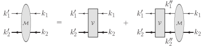
Figure 1: The diagram for the Bethe-Salpeter equaiton. The thick and thin lines are for particles 1 and 2, respectively.

In this work, a quasipotential approximation will be applied to reduce the four-dimensional Bethe-Salpeter equation to a three-dimensional one. Here the covariant spectator theory will be applied as shown in Appendix A, in which the heavier meson, particle 2, is put on shell. After multiplying the polarized vector on both sides of the equation, we have

$${\cal M}_{\lambda^{\prime},\lambda}({\bm{p}}^{\prime},{\bm{p}}) = {\cal V}_{\lambda^{\prime}\lambda}({\bm{p}}^{\prime},{\bm{p}})+\sum_{\lambda^{\prime\prime}}\int\frac{d^{3}p^{\prime\prime}}{(2\pi)^{3}}$$ (2)

$$\cdot {\cal V}_{\lambda^{\prime}\lambda^{\prime\prime}}({\bm{p}}^{\prime},{\bm{p}}^{\prime\prime})G_{0}({\bm{p}}^{\prime\prime}){\cal M}_{\lambda^{\prime\prime}\lambda}({\bm{p}}^{\prime\prime},{\bm{p}}),\quad$$

where ${\bm{p}}$, ${\bm{p}}^{\prime}$ and ${\bm{p}}^{\prime\prime}$ are the momenta of constituent 2. And the potential ${\cal V}_{\lambda^{\prime}\lambda}({\bm{p}}^{\prime},{\bm{p}})=\epsilon^{\mu*}_{\lambda^{\prime}}({\bm{p}}^{\prime}){\cal V}_{\mu\nu}({\bm{p}}^{\prime},{\bm{p}})\epsilon^{\nu}_{\lambda}({\bm{p}})$.

To reduce the Bethe-Salpeter equation to a one-dimensional equation, we apply the partial wave expansion as shown in Appendix B. The partial wave Bethe-Salpeter equation with fixed parity reads as,

$${\cal M}^{J^{P}}_{\lambda^{\prime}\lambda}({\rm p}^{\prime},{\rm p}) = {\cal V}^{J^{P}}_{\lambda^{\prime},\lambda}({\rm p}^{\prime},{\rm p})+\sum_{\lambda^{\prime\prime}}\int\frac{{\rm p}^{\prime\prime 2}d{\rm p}^{\prime\prime}}{(2\pi)^{3}}$$ (3)

$$\cdot {\cal V}^{J^{P}}_{\lambda^{\prime}\lambda^{\prime\prime}}({\rm p}^{\prime},{\rm p}^{\prime\prime})G_{0}({\rm p}^{\prime\prime}){\cal M}^{J^{P}}_{\lambda^{\prime\prime}\lambda}({\rm p}^{\prime\prime},{\rm p}).\quad\quad$$

Note that the sum extends only over non-negative $\lambda^{\prime\prime}$, and a factor $1/\sqrt{2}$ has been included in the scattering amplitude and potential for zero helicity. The potential is defined as

$${\cal V}_{\lambda^{\prime}\lambda}^{J^{P}}({\rm p}^{\prime},{\rm p}) = 2\pi\int d\cos\theta~{}[d^{J}_{\lambda\lambda^{\prime}}(\theta){\cal V}_{\lambda^{\prime}\lambda}({\bm{p}}^{\prime},{\bm{p}})$$ (4)

$$+ \eta d^{J}_{-\lambda\lambda^{\prime}}(\theta){\cal V}_{\lambda^{\prime}-\lambda}({\bm{p}}^{\prime},{\bm{p}})],$$

where the momenta are chosen as $k_{1}=(W-E,0,0,-{\rm p})$, $k_{2}=(E,0,0,{\rm p})$ and $k^{\prime}_{1}=(W-E^{\prime},-{\rm p}^{\prime}\sin\theta,0,-{\rm p}^{\prime}\cos\theta)$, $k^{\prime}_{2}=(E^{\prime},{\rm p}^{\prime}\sin\theta,0,{\rm p}^{\prime}\cos\theta)$ with ${\rm p}=|{\bm{p}}|$ in order to avoid confusion with the four-momentum $p$.

The above equation can be related to the Lippmann-Schwinger equations used by Oset $et\ al.$, if the potential kernel ${\cal V}$ is only dependent on the square of the momentum of the system $s=P^{2}$ and the $G_{0}$ is chosen as the one used in Ref. Oset and Ramos (1998). A cutoff regularization has been introduced in the integration of the propagator in Ref. Oset and Ramos (1998), and it is related to a dimensional regularization. Since in our formalism, the integration is on the potential also the only cutoff regularization is practical here. In this work we will adopt an exponential regularization instead of cutoff regularization by introducing a form factor in the propagator as

$$G_{0}({\rm p})\to G_{0}({\rm p})\left[e^{-(k_{1}^{2}-m_{1}^{2})^{2}/\Lambda^{4}}\right]^{2}.$$ (5)

Here particle 2 is not involved in the form factor due to its on-shell-ness. The exponential regularization used here can be seen as a softer version of the cutoff regularization in Ref.  Oset and Ramos (1998), where the momentum $\rm p$ is cutoff at a certain value ${\rm p}_{max}$. The cutoff $\Lambda$ plays an analogous role to the cutoff ${\rm p}_{max}$ of cutoff regularization. It can also be understood as a form factor in exponential form for the charmed mesons to reflect the internal structure of the hadron and to make the integration convergent. It is consistent with the OBE model where a form factor is usually added for the off-shell particle.

III The potential

In Ref. He (2014), it was explained explicitly how to construct a potential for states with definite isospin under SU(3) symmetry with the corresponding flavor wave functions Sun $et~{}al.$ (2011)

$$|Z_{D\bar{D}^{*}}^{+}\rangle_{I=1} = \frac{1}{\sqrt{2}}\big{(}|D^{*+}\bar{D}^{0}\rangle+c|D^{+}\bar{D}^{*0}\rangle\big{)},$$

$$|Z_{D\bar{D}^{*}}^{-}\rangle_{I=1} = \frac{1}{\sqrt{2}}\big{(}|D^{*-}\bar{D}^{0}\rangle+c|D^{-}\bar{D}^{*0}\rangle\big{)},$$

$$|Z_{D\bar{D}^{*}}^{0}\rangle_{I=1} = \frac{1}{2}\Big{[}\big{(}|D^{*+}D^{-}\rangle-|D^{*0}\bar{D}^{0}\rangle\big{)}$$

$$+ c\big{(}|D^{+}D^{*-}\rangle-|D^{0}\bar{D}^{*0}\rangle\big{)}\Big{]},$$

$$|Z_{D\bar{D}^{*}}^{0}\rangle_{I=0} = \frac{1}{2}\Big{[}\big{(}|D^{*+}D^{-}\rangle+|D^{*0}\bar{D}^{0}\rangle\big{)}$$ (6)

$$+ c\big{(}|D^{+}D^{*-}\rangle+|D^{0}\bar{D}^{*0}\rangle\big{)}\Big{]},$$

where $c=\pm$ corresponds to $C$-parity $C=\mp$ respectively. For the isovector state the $c$ is related to the $G$-parity.

Basically, the strong interaction should be described by gluon and quark freedoms. If the distance between two hadrons is large, the interaction will appear as meson exchange, that is, the OBE model. Many efforts have been made to study the connection between QCD and the OBE model. For example, in Refs. Simonov (2011); Danilkin $et~{}al.$ (2012) after integrating out quark degrees of freedom in the effective Lagrangian, one obtains the chiral effective Lagrangian for mesons. Though there is still not particularly convincing about the connection, as a phenomenological model the people’s confidence about the OBE model arises from the successes of its applications to the deuteron, such as the CD-Bonn model Machleidt $et~{}al.$ (1987) and the Gross model Gross and Stadler (2010), and the constituent quark model by Riska and Glozman Glozman and Riska (1996). If the X(3872) is interpreted as a molecular state, it should have a radius of about 7 fm, as estimated by Close and Page Close and Page (2004). For a resonance above the threshold, it is reasonable to assume the interaction is at a large distance. Hence, the OBE model will be adopted to describe the $D\bar{D}^{*}$ interaction in this work.

It seems strange to include the vector-meson exchanges, which mainly take effect at short distances. However, we should remind the reader that a short-distance interaction does not mean an interaction only at short distances. The vector-meson exchange will have some remnant at long distances. It is also can be understood as indicating that there is some possibility that the two hadrons are close to each other. If the interaction from the vector-meson exchange is large enough, it will have a considerable remnant at long distances. Based on this consideration, the vector-meson exchanges are also included in the OBE model. At short distances, the studies in the constituent quark model suggests the gluon exchange contribution can be replaced by the contribution from vector-meson exchanges Dai $et~{}al.$ (2003); He and Dong (2003). Therefore, vector-meson exchanges will be included in the calculation in this work instead of gluon exchange.

There exist two types of diagram namely, the direct diagram and the cross diagram (see Fig. 2), as in a conventional OBE potential model Sun $et~{}al.$ (2011, 2012). In the cross diagram, the final particles are alternated. With such alternation, the propagator is the same for different components in a SU(3) state, such as $|D^{*+}\bar{D}^{0}\rangle$ and $|D^{+}\bar{D}^{*0}\rangle$ for the positive-charge state, so that the equations for different components are reduced to one equation under S(3) symmetry He (2014).

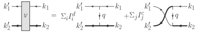
Figure 2: The potential including both direct and cross diagrams. $I^{d}_{i}$ and $I^{c}_{i}$ are the isospin factors for direct and cross diagrams, respectively.

To write the potential, we adopt the effective Lagrangians of the pseudoscalar and vector mesons with heavy flavor mesons from the heavy quark effective theory  Colangelo $et~{}al.$ (2004); Casalbuoni $et~{}al.$ (1997). The potential kernels ${\cal V}$ from vector-meson ($\mathbb{V}$) exchange, pseudoscalar-meson ($\mathbb{P}$) exchange, and scalar-meson ($\sigma$) exchange have been given in Ref. He (2014) as

$${\cal V}^{Direct}_{\mathbb{V}} = i\frac{\beta^{2}g^{2}_{V}}{2}\frac{(k_{2}+k^{\prime}_{2})\cdot(k_{1}+k^{\prime}_{1})~{}\epsilon_{2}\cdot\epsilon^{\prime}_{2}}{q^{2}-m_{\mathbb{V}}^{2}},$$

$${\cal V}^{Direct}_{\sigma} = i4g^{2}_{\sigma}m_{P}m_{P^{*}}\frac{\epsilon_{2}\cdot\epsilon^{\prime}_{2}}{q^{2}-m^{2}_{\sigma}},$$

$${\cal V}^{Cross}_{\mathbb{V}} = i2\lambda^{2}g^{2}_{V}\varepsilon_{\lambda\alpha\beta\mu}(k_{2}+k^{\prime}_{1})^{\lambda}q^{\alpha}\epsilon_{2}^{\mu}~{}$$

$$\cdot \varepsilon_{\lambda^{\prime}\alpha^{\prime}\beta\nu}(k_{1}+k^{\prime}_{2})^{\lambda^{\prime}}q^{\alpha^{\prime}}\epsilon^{\prime\nu}_{2}\frac{1}{q^{2}-m_{\mathbb{V}}^{2}},$$

$${\cal V}^{Cross}_{\mathbb{P}} = i\frac{4g^{2}m_{P}m_{P^{*}}}{f^{2}_{\pi}}\frac{k^{\prime}_{1}\cdot\epsilon_{2}k_{1}\cdot\epsilon^{\prime}_{2}}{q^{2}-m^{2}_{\mathbb{P}}},$$ (7)

where the momenta $k^{(^{\prime})}_{1,2}$ and $q$ are defined as in Fig. 2. Here The $\epsilon^{(^{\prime})}_{2}$ is the polarization vector for the initial or final particle 2. $m_{\mathbb{P}}$, $m_{\mathbb{V}}$ and $m_{\sigma}$ are the masses for the exchange pseudoscalar, vector, and sigma mesons. In the OBE model, the masses of all mesons used are from the PDG Olive $et~{}al.$ (2014). The $\sigma$ meson is seen as a particle with a mass 475 MeV, which is the center value suggested by the PDG.

In the OBE model, we will adopt the physical values of the coupling constants. How to determine the coupling constants has been discussed in the heavy quark effective theory Casalbuoni $et~{}al.$ (1997). The coupling constant $g$ for the pseudoscalar exchange is extracted from the experimental width of $D^{*+}$ as $g=0.59$ Isola $et~{}al.$ (2003). The parameter $\beta$ for the vector meson was fixed as $\beta=0.9$ by the vector-meson dominance mechanism and $\lambda=0.56$ GeV^-1 was obtained by comparing the form factor obtained by lattice QCD with the one calculated by the light-cone sum rule  Colangelo $et~{}al.$ (2004). The coupling constant $g_{\sigma}=g_{\pi}/(2\sqrt{6})$ with $g_{\pi}=3.73$ was given in Ref. Falk and Luke (1992).

A form factor is introduced to compensate the off-shell effect of the exchange meson as $f(q^{2})=(\frac{\Lambda^{2}}{\Lambda^{2}-q^{2}})^{4}$. It is different from the one used in the propagator [see Eq. (5)] , which is usually used in a case where the off-shell particle has possibility $q^{2}=\Lambda^{2}$, to avoid an unnecessary pole arising from the form factor. The cutoff can be related to the radius of the hadron as

$$r^{2}=-\frac{6}{F(0)}\frac{d}{dq^{2}}F(q^{2})|_{q^{2}=0}.$$ (8)

With Eq. (8), the cutoffs in two types of form factors have relation $\Lambda\approx 5/r$. If we assume the mesons have radii of about 0.5 fm, the cutoff is about 2 GeV. Here the momenta for the exchange mesons are defined as $q=k^{\prime}_{2}-k_{2}$ and $q=k^{\prime}_{1}-k_{2}$ for direct and cross diagrams, respectively. In the propagator of the meson exchange we make a replacement $q^{2}\to-|q^{2}|$ to remove the unphysical singularities, as in Ref. Gross and Stadler (2008).

In Ref. Aceti $et~{}al.$ (2014), it was suggested that the $J/\psi$ exchange is important in the $D\bar{D}^{*}$ interaction. And the potential was written in the local hidden gauge approach with heavy quark spin symmetry. In this work, the couplings of heavy-light charmed mesons to $J/\psi$ are written with help of the heavy quark effective theory as Casalbuoni $et~{}al.$ (1997); Oh $et~{}al.$ (2001)

$${\cal L}_{D^{*}_{(s)}\bar{D}^{*}_{(s)}J/\psi} = -ig_{D^{*}_{(s)}D^{*}_{(s)}\psi}\big{[}\psi\cdot\bar{D}^{*}\overleftrightarrow{\partial}\cdot D^{*}$$

$$- \psi^{\mu}\bar{D}^{*}\cdot\overleftrightarrow{\partial}^{\mu}{D}^{*}+\psi^{\mu}\bar{D}^{*}\cdot\overleftrightarrow{\partial}D^{*\mu})\big{]},$$

$${\cal L}_{D_{(s)}^{*}\bar{D}_{(s)}J/\psi} = g_{D^{*}_{(s)}D_{(s)}\psi}\,\,\epsilon_{\beta\mu\alpha\tau}\partial^{\beta}\psi^{\mu}(\bar{D}\overleftrightarrow{\partial}^{\tau}D^{*\alpha}+\bar{D}^{*\alpha}\overleftrightarrow{\partial}^{\tau}D),$$

$${\cal L}_{D_{(s)}\bar{D}_{(s)}J/\psi} = ig_{D_{(s)}D_{(s)}\psi}\psi\cdot\bar{D}\overleftrightarrow{\partial}D,$$ (9)

where the couplings are related to a single parameter $g_{2}$ as

$$\frac{g_{D^{*}D^{*}\psi}}{m_{D^{*}}}=\frac{g_{D_{(s)}D_{(s)}\psi}}{m_{D}}=g_{D^{*}_{(s)}D_{(s)}\psi}=2g_{2}\sqrt{m_{\psi}},$$ (10)

with $g_{2}={\sqrt{m_{\psi}}}/({2m_{D}f_{\psi}})$ with $f_{\psi}=405$ MeV.

With the above Lagrangians, the potential kernel for $J/\psi$ exchange is written as,

$${\cal V}^{Direct}_{J/\psi} = -ig_{D^{*}D^{*}J/\psi}g_{DDJ/\psi}[\epsilon^{\prime}_{2}\cdot(k_{1}+k^{\prime}_{1})~{}\epsilon_{2}\cdot(k_{2}+k^{\prime}_{2})$$

$$+ \epsilon^{\prime}_{2}\cdot(k_{2}+k^{\prime}_{2})~{}\epsilon_{2}\cdot(k_{1}+k^{\prime}_{1})$$

$$- (k_{2}+k^{\prime}_{2})\cdot(k_{1}+k^{\prime}_{1})~{}\epsilon^{\prime}_{2}\cdot\epsilon_{2}]\frac{1}{q^{2}-m_{J/\psi}^{2}},$$

$${\cal V}^{Cross}_{J/\psi} = ig_{DD^{*}J/\psi}^{2}~{}\varepsilon_{\lambda\alpha\beta\mu}(k_{2}+k^{\prime}_{1})^{\lambda}q^{\alpha}\epsilon_{2}^{\mu}~{}$$ (11)

$$\cdot \varepsilon_{\lambda^{\prime}\alpha^{\prime}\beta\nu}(k_{1}+k^{\prime}_{2})^{\lambda^{\prime}}q^{\alpha^{\prime}}\epsilon^{\prime\nu}_{2}\frac{1}{q^{2}-m_{J/\psi}^{2}}.$$

We would like to point out that the potentials obtained by the heavy quark effective theory are comparable to the ones obtained from the chiral Lagrangian in Ref. Aceti $et~{}al.$ (2014) after a nonrelativization. For example, the potential kernel for the $J/\psi$ exchange can be rewritten as

$${\cal V}^{Direct}_{J/\psi} = -\frac{g_{D^{*}D^{*}J/\psi}g_{DDJ/\psi}}{m_{J/\psi}^{2}}(k_{2}+k^{\prime}_{2})\cdot(k_{1}+k^{\prime}_{1})~{}{\bm{\epsilon}}^{\prime}_{2}\cdot{\bm{\epsilon}}_{2},\ \ \$$ (12)

with ${g_{D^{*}D^{*}J/\psi}g_{DDJ/\psi}}/{m_{J/\psi}^{2}}=7.04$ in this work and

$${\cal V}^{Direct}_{J/\psi} = -\frac{{\cal C}_{ij}}{4f^{2}}(k_{2}+k^{\prime}_{2})\cdot(k_{1}+k^{\prime}_{1})~{}{\bm{\epsilon}}^{\prime}_{2}\cdot{\bm{\epsilon}}_{2},\ \$$ (13)

with ${{\cal C}_{ij}}/{4f^{2}}=6.89$ in Ref. Aceti $et~{}al.$ (2014). The main difference between our work and Ref. Aceti $et~{}al.$ (2014) is that a form factor is added not only to the light pseudoscalar-meson exchanges but also to the $J/\psi$ exchange, which will suppress the contribution from $J/\psi$ exchange.

The flavor factors $I_{i}^{d}$ and $I_{i}^{c}$ for direct and cross diagrams are presented in Table 1. The cancellation of the $\rho$ and $\omega$ meson exchanges happens in the isovector sector as suggested by the isospin factor listed in Table 1, which leads to a shortage of the short-range interaction in that sector if the $J/\psi$ exchange is absent.

Table 1: The isospin factors $I_{i}^{d}$ and $I_{i}^{c}$ for direct and cross diagrams and different exchange mesons.

	Direct diagram				Crossed diagram
	$\rho$	$\omega$	$J/\psi$	$\sigma$	$\pi$	$\eta$	$\rho$	$\omega$	$J/\psi$
$[PP^{*}]^{T}$	$-\frac{1}{2}$	$\frac{1}{2}$	1	1	$-{\textstyle{1\over 2}}c$	$\frac{1}{6}c$	$-{\textstyle{1\over 2}}c$	${\textstyle{1\over 2}}c$	$c$
$[PP^{*}]^{S}$	${\textstyle{3\over 2}}$	${\textstyle{1\over 2}}$	1	1	$\frac{3}{2}c$	$\frac{1}{6}c$	${\textstyle{3\over 2}}c$	$\frac{1}{2}c$	$c$

IV Numerical results

In this work, we will search the poles of the scattering amplitude ${\cal M}$ from the $D\bar{D}^{*}$ interaction which is described by the potential kernel obtained in the above section. The scattering amplitude is obtained by solving the Bethe-Salpeter equation.

IV.1 Numerical solution of the Bethe-Salpeter equation

Before solving the one-dimensional partial wave Bethe-Salpeter equation numerically, we need to deal with the pole in $G_{0}({\rm p})$ as (here the notation $J^{P}$ is omitted)

$$i{\cal M}({\rm p},{\rm p}^{\prime})=i{\cal V}({\rm p},{\rm p}^{\prime})$$ (14)

$$+ \int\frac{{\rm p}^{\prime\prime 2}d{\rm p}^{\prime\prime}}{(2\pi)^{3}}i{\cal V}({\rm p},{\rm p}^{\prime\prime})G_{0}({\rm p}^{\prime\prime})i{\cal M}({\rm p}^{\prime\prime},{\rm p^{\prime}})$$

$$- i{\cal V}({\rm p},{{\rm p}}_{o}^{\prime\prime})[\int\frac{d{\rm p}^{\prime\prime}}{(2\pi)^{3}}\frac{A({\rm p}^{\prime\prime}_{o})}{{\rm p}^{\prime\prime 2}-{\rm p}^{\prime\prime 2}_{o}}+i\frac{{\rm p}^{\prime\prime 2}_{o}\delta\bar{G}_{0}({\rm p}^{\prime\prime}_{o})}{8\pi^{2}}]$$

$$\cdot i{\cal M}({\rm p}^{\prime\prime}_{o},{\rm p}^{\prime})\theta(s-m_{1}-m_{2}),$$

with

$$A({\rm p}^{\prime\prime}_{o})=[{\rm p}^{\prime\prime 2}({\rm p}^{\prime\prime 2}-{\rm p}^{\prime\prime 2}_{o})G_{0}({\rm p}^{\prime\prime})]_{{\rm p}^{\prime\prime}\to{\rm p}^{\prime\prime}_{o}}=-\frac{{\rm p}^{\prime\prime 2}_{o}}{2W},$$

$$\delta\bar{G}_{0}({\rm p}^{\prime\prime})\delta({\rm p}^{\prime\prime}-{\rm p}^{\prime\prime}_{o})=\delta(G_{0}({\rm p})^{\prime\prime})=\frac{1}{4W{\rm p}^{\prime\prime}_{o}}\delta({\rm p}^{\prime\prime}-{\rm p}^{\prime\prime}_{o}),\quad\quad$$ (15)

with ${\rm p}^{\prime\prime}_{o}=\frac{1}{2W}\sqrt{[W^{2}-(M+m)^{2}][W^{2}-(M-m)^{2}]}$.

To solve the integral equation, we discrete the momenta ${\rm p}$, ${\rm p}^{\prime}$, and ${\rm p}^{\prime\prime}$ by the Gauss quadrature with wight $w({\rm p}_{i})$ and have

$${M}_{ik} = {V}_{ik}+\sum_{j=0}^{N}{V}_{ij}G_{j}{M}_{jk},$$ (16)

where $i$ is absorbed in $M$ or $V$. The discreted propagator is of a form

$$G_{j>0} = \frac{w({\rm p}^{\prime\prime}_{j}){\rm p}^{\prime\prime 2}_{j}}{(2\pi)^{3}}G_{0}({\rm p}^{\prime\prime}_{j}),$$

$$G_{j=0} = -\frac{i{\rm p}^{\prime\prime}_{o}}{32\pi^{2}W}+\sum_{j}\left[\frac{w({\rm p}_{j})}{(2\pi)^{3}}\frac{{\rm p}^{\prime\prime 2}_{o}}{2W{({\rm p}^{\prime\prime 2}_{j}-{\rm p}^{\prime\prime 2}_{o})}}\right].\quad\quad$$ (17)

In this work, we will search the poles from the amplitude of elastic scattering where the initial and final particles are on shell. The scattering amplitude is

$$M=M_{00}=\sum_{j}[(1-{V}G)^{-1}]_{0j}V_{j0}.$$ (18)

The pole can be searched by variation of $z$ to satisfy

$$|1-V(z)G(z)|=0,$$ (19)

where $z=E_{R}+i\Gamma/2$ equals the meson-baryon energy $W$ at the real axis. Since $z=\sqrt{m_{1}^{2}+{\rm p}^{2}}+\sqrt{m_{2}^{2}+{\rm p}^{2}}$, the $\rm p$-plane corresponds to two Reimann sheets for $z$. A bound state is located in the first Reimann sheet while a resonance is located in the second Reimann sheet with Im(p)$<$0. Since only one channel is considered in this work, the bound state is located at the real axis of the $z$ complex plane, while the resonance will deflect the real axis to the complex plane.

IV.2 Bound state from $D\bar{D}^{*}$ interaction with a $\Lambda$ scan

There exist two types of pole, namely bound state and resonance. First, we will make a $\Lambda$ scan from 0.8 GeV to 4 GeV to find the bound state from the $D\bar{D}^{*}$ interaction. The pole of a bound state from $D\bar{D}^{*}$ interaction is located at the real axis.

Table 2: The position of the bound state from the $D\bar{D}^{*}$ interaction at the real axis $Re(z)=W$ with a $\Lambda$ scan. The second and third columns are for the full model. The results without the $J/\psi$ exchange are listed in the fourth and fifth columns and compared with the results in Ref. He (2014). The $J/\psi$ (I) in the eighth and ninth columns and $J/\psi$ (II) in tenth and eleventh columns are for the results from only $J/\psi$ exchange with and without form factor. The cutoff $\Lambda$ and energy $W$ are in units of GeV.

	Full model		No $J/\psi$		Ref. He (2014)		$J/\psi$ (I)		$J/\psi$ (II)
$I^{G}(J^{PC})$	$\Lambda$	$W$	$\Lambda$	$W$	$\Lambda$	$W$	$\Lambda$	$W$	$\Lambda$	$W$
$0^{-}(0^{--})$	–	–	–	–	–	–	–	–	–	–
$0^{+}(0^{-+})$	–	–	–	–	–	–	–	–	–	–
$0^{-}(1^{--})$	–	–	–	–	–	–	–	–	–	–
$0^{+}(1^{-+})$	–	–	–	–	–	–	–	–	–	–
$0^{-}(1^{+-})$	1.0	3.864	1.0	3.868	1.3	3.876	–	–	2.5	3.867
	1.2	3.848	1.2	3.854	1.4	3.870	–	–	2.6	3.850
$0^{+}(1^{++})$	1.9	3.873	1.9	3.875	2.0	3.876	–	–	3.9	3.875
	2.4	3.871	2.4	3.874	2.4	3.872	–	–	4.0	3.836
$1^{+}(0^{-})$	–	–	–	–	–	–	–	–	–	–
$1^{-}(0^{-})$	–	–	–	–	–	–	–	–	–	–
$1^{+}(1^{-})$	–	–	–	–	–	–	–	–	–	–
$1^{-}(1^{-})$	–	–	–	–	–	–	–	–	–	–
$1^{+}(1^{+})$	3.0	3.874	–	–	–	–	–	–	2.4	3.875
	3.3	3.858	–	–	–	–	–	–	2.5	3.867
$1^{-}(1^{+})$	–	–	–	–	–	–	–	–	–	–

One can find that the $J/\psi$ exchange plays a more important role in the isoscalar sector than in the isovector sector, where the short-range interaction is absent due to the cancellation between $\rho$ and $\omega$ exchanges in the isoscalar sector, as shown in Table 1. As expected, the results without the $J/\psi$ exchange are also close to those obtained from the solution of a Bethe-Salpeter equation for the vertex in Ref. He (2014). The results with only the $J/\psi$ exchange are also listed in Table 2. There is no bound state found for the $J/\psi$ exchange with form factor [labeled as $J/\psi$ (I)], while if the form factor is removed [labeled as $J/\psi$ (II)], the bound state is found as in the full model, which indicates the form factor weakens the contribution from the $J/\psi$ exchange.

In the isoscalar vector, there exist hidden charmed bound states with $I^{G}(J^{PC})=0^{-}(1^{+-})$ and $0^{-}(1^{++})$ with cutoffs about 1 GeV and 2 GeV, respectively. The $D\bar{D}^{*}$ bound state with $0^{+}(1^{++})$ can be related to the $X(3872)$. In the isovector sector, a bound state with $1^{+}(1^{+})$ can be found with a larger cutoff at about 3 GeV.

IV.3 The $Z_{c}(3900)$ as a resonance

In physics, the cutoff in the $D\bar{D}^{*}$ interaction should be same for different quantum numbers. Usually, a decrease of the cutoff will lead to a weaker interaction, and vice versa. As stated in the scattering theory, when interaction weakens, the bound state runs to the threshold and becomes a resonance if the interaction is still strong enough. If the cutoff is increased to 3 GeV, the pole with $0^{+}(1^{++})$ will move to about 3650 MeV, which is very far from the experimental mass of $X(3872)$. Hence, we decrease the cutoff $\Lambda$ for $1^{+}(1^{+})$ from about 3 GeV to 2.4 GeV with which a bound state which has quantum number $0^{+}(1^{++})$ is found at 3.871 GeV. A pole with $1^{+}(1^{+})$ is produced slightly higher than the $D\bar{D}^{*}$ threshold with a cutoff $\Lambda=2.4$ GeV as shown in the upper panel of Fig. 3. It is located at $z=3876+i5$ MeV and can be identified with the charged charmonium-like state $Z_{c}(3900)$ observed in BESIII.

Obviously, the position of the pole is below the experiment masses of $Z_{c}(3900)$, 3883.9$\pm 1.5\pm 4.2$ MeV in the $D\bar{D}^{*}$ channel and $3899\pm 3.6\pm 4.9$ MeV in the $\pi^{-}J/\psi$ channel Olive $et~{}al.$ (2014). The experimental mass is obtained by fitting the invariant mass spectrum. As shown in the middle and lower panels of Fig. 3, the invariant mass spectrum of the $D\bar{D}^{*}$ channel is presented and compared with the experimental results released by the BESIII Collaboration Ablikim $et~{}al.$ (2014).

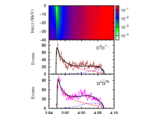
Figure 3: (color online) The $|1-G(z)V(z)|$ for $I^{G}(J^{PC})=1^{+}(1^{+})$ in the complex energy plane (upper panel) and the $D^{0}D^{*-}$ (middle panel) and $D^{+}\bar{D}^{*0}$ (lower panel) invariant mass spectra. The abscissa axis $Re(z)$ represents the corresponding $D\bar{D}^{*}$ invariant mass $W$ in units of GeV. The solid, dotted, and dashed lines are for results with the full model, the resonance contribution, and the background, respectively. The experimental results are from BESIII Ablikim $et~{}al.$ (2014).The theoretical results are normalized to the experiment.

The invariant mass distribution is given approximately as Hyodo $et~{}al.$ (2003); Aceti $et~{}al.$ (2014)

$$\frac{d\sigma}{dW}=C|{M}^{1^{+}}|^{2}\lambda^{\textstyle{1\over 2}}(W^{2},M^{2},m^{2})\lambda^{\textstyle{1\over 2}}(\tilde{W}^{2},W^{2},m_{3}^{2})/W,$$ (20)

where $M^{1^{+}}$ is the scattering amplitude obtained from the Bethe-Salpeter eqaution as defined in Eq. (18), $\tilde{W}$ is total energy of the process, and $m_{3}$ is the third final particle $\pi$ Hemingway (1985); Aceti $et~{}al.$ (2014). A background spectrum is also included as in Refs. Ablikim $et~{}al.$ (2014); Aceti $et~{}al.$ (2014),

$$f_{bkg}(W)=a(W-M_{min})^{c}(M_{max}-W)^{d},$$ (21)

where $M_{min}$ and $M_{max}$ are the minimum and maximum kinematically allowed masses. The general constant $C$ in Eq. (20), and the general constant $a$ and exponents $c$ and $d$ in Eq. (21) are free parameters adjusted to reproduce the experimental data.

The experimental data are well reproduced with the resonance contribution plus a background. A peak is found at 3881 MeV which is higher than the position of the pole of the resonance but closer to the experimental results 3883.9$\pm 1.5\pm 4.2$ MeV in the $D\bar{D}^{*}$ channel Ablikim $et~{}al.$ (2014). We would like to note that due to the pole’s nearness to the threshold the contribution from the $Z_{c}(3900)$ in our model does not have a standard Breit-Wigner form, which was adopted in the experimental fitting  Ablikim $et~{}al.$ (2014). The nearness also results in a relatively large tail of the resonance at higher energies. These differences lead to a background contribution, which is quite different from the one in Ref. Ablikim $et~{}al.$ (2014) to be used to reproduce the invariant mass spectrum.

V Summary

In this work, the $D\bar{D}^{*}$ interaction is studied within the OBE model, including the contribution from light meson exchanges plus the short-range $J/\psi$ exchange. The scattering amplitude is calculated within a Bethe-Salpeter equation approach, and the poles near the $D\bar{D}^{*}$ threshold are searched. It is found that the charged charmonium-like state $Z_{c}(3900)$ can be interpreted a resonance above the threshold from the $D\bar{D}^{*}$ interaction.

In the isoscalar sector, the poles are found under the $D\bar{D}^{*}$ threshold and have the quantum numbers $I^{G}(J^{PC})=0^{-}(1^{+-})$ and $0^{+}(1^{++})$. If the $J/\psi$ exchange is excluded, the position of the pole is almost unaffected. In the isovector sector, where the short-range contributions from $\omega$ and $\rho$ exchanges are canceled, a bound state is found with $I^{G}(J^{P})=1^{+}(1^{+})$. It disappears if the $J/\psi$ exchange is removed. The results show that the short-range $J/\psi$ exchange, which is not included in the conventional one-boson exchange model, is important to provide an attractive interaction to produce the pole in the isovector sector.

If a cutoff $\Lambda=2.4$ GeV is adopted with which a pole carrying the quantum number of the $X(3872)$ is produced at an energy of about 3871 MeV, the pole for the bound state with $1^{+}(1^{+})$ runs across the threshold to a second Rienman sheet and becomes a resonance at $3876+i5$ MeV, which can be identified with the $Z_{c}(3900)$. The line shape of the invariant mass spectrum in the $D\bar{D}^{*}$ channel is also investigated and the experimental results by the BESIII Collaboration can be reproduced. A peak is found in the $D\bar{D}^{*}$ invariant mass spectrum at about 3881 MeV, which is higher than the resonance pole but closer to the experimental values.

Note: Just after the paper was submitted, we noticed a related work released in arXiv, in which the author also found a second-sheet pole in studying elastic $D\bar{D}^{*}$ scatteringZhou and Xiao (2015).

Appendix A The quasipotential approximation of the Bethe-Salpeter equation

It is popular to reduce the Bethe-Salpeter equation from a four-dimensional integral equation to a three-dimensional equation by quasipotential approximation. In principle, infinite choices can be applied to make the quasipotential approximation. The popular methods used in literature include the BSLT approximation, the K-matrix method, the instantaneous approximation, and the covariant spectator theory (CST)  Blankenbecler and Sugar (1966); Shklyar $et~{}al.$ (2005); Guo and Wu (2007); Gross $et~{}al.$ (1992); Gross and Stadler (2008); He (2014, 2015); Nieuwenhuis and Tjon (1996).

The reduced propagator $G$ under quasipotential approximations should satisfy the unitary condition, i.e., the relation

$$G-G^{\dagger}=2\pi i\delta((\eta_{1}(s)P+k)^{2}-m^{2})\delta((\eta_{2}(s)P-k)^{2}-m^{2}),\ \ \$$ (22)

where $k_{1}=\eta_{1}(s)P+k$, $k_{2}=\eta_{2}(s)-k$, and $m_{1,2}$ are the momenta and mass of constituents 1 and 2 with $\eta_{1}(s)+\eta_{2}(s)=1$ and $s=P^{2}$. One can define $\eta_{1,2}=\epsilon_{1,2}/(\epsilon_{1}+\epsilon_{2})$ with $\epsilon_{1,2}(s)=(s+m_{1,2}^{2}-m_{2,1}^{2})/2\sqrt{s}$. Now we have many choices to write the propagator. The most popular form of propagator is Hung $et~{}al.$ (2001); Zakout (1996); He and Lü (2013)

$$G = 2\pi\int\frac{ds^{\prime}}{s^{\prime}-s+i\epsilon}h(s^{\prime},s)$$ (23)

$$\cdot \delta([\eta^{\prime}_{1}(s^{\prime})P^{\prime}+k]^{2}-m_{1}^{2})~{}\delta([\eta^{\prime}_{2}(s^{\prime})P^{\prime}-k]^{2}-m_{2}^{2}),\ \$$

where $P^{\prime}=\sqrt{s^{\prime}/s}P$. It is random to some extent to choose $h(s^{\prime},s)$ . The $h$ function is chosen as $h(s^{\prime}-s)=1$ with $\eta^{\prime}(s^{\prime})=\eta(s^{\prime})$ for the BSLT formalisms,. In the CST, $h(s^{\prime},s)=(\sqrt{s^{\prime}}+\sqrt{s})/\sqrt{s^{\prime}}$, with $\eta^{\prime}_{1}(s^{\prime})=\eta_{1}(s)\sqrt{s/s^{\prime}}$ and $\eta^{\prime}_{2}(s^{\prime})=1-\eta_{1}(s)\sqrt{s/s^{\prime}}$.

Eqation (23) is quite far from exhausting all possible three-dimensional reductions. For example, the widely used instantaneous approximation has

$$G = \int dk_{0}\frac{-1}{(k_{1}^{2}-m_{1}^{2}+i\epsilon)(k_{2}^{2}-m_{2}^{2}+i\epsilon)}$$ (24)

$$= i\pi\frac{(E_{1}({\bm{p}})+E_{2}({\bm{p}}))/E_{1}({\bm{p}})E_{2}({\bm{p}})}{W^{2}-(E_{1}({\bm{p}})+E_{2}({\bm{p}}))^{2}},$$

which satisfies the unitary condition also.

As in Ref. He (2014), the covariant spectator theory Gross $et~{}al.$ (1992); Gross and Stadler (2008) is adopted to make the quasipotential approximation to reduce the four-dimensional Bethe-Salpeter equation to a three-dimensional equation in the current work. Written down in the center-of-mass frame where $P=(W,{\bm{0}})$, the propagator in the CST is

$$G = 2\pi i\frac{\delta^{+}(k_{2}^{~{}2}-m_{2}^{2})}{k_{1}^{~{}2}-m_{1}^{2}}$$ (25)

$$= 2\pi i\frac{\delta^{+}(k^{0}_{2}-E_{2}({\bm{p}}))}{2E_{2}({\bm{p}})[(W-E_{2}({\bm{p}}))^{2}-E_{1}^{2}({\bm{p}})]},$$

where $k_{1}=(k_{1}^{0},-\bm{p})=(W-E_{2}({\bm{p}}),-\bm{p})$ and$k_{2}=(k_{2}^{0},\bm{p})=(E_{2}({\bm{p}}),\bm{p})$ with $E_{1,2}({\bm{p}})=\sqrt{m_{1,2}^{~{}2}+|\bm{p}|^{2}}$. In our formalism a definition $G_{0}=G/2\pi$ is used for convenience.

Appendix B The partial wave expansion and the amplitudes with fixed parity

The partial wave expansion of the scattering amplitude ${\cal M}$ in Eq. (2) is Chung (2014)

$${\cal M}_{\lambda^{\prime}\lambda}({\bm{p}}^{\prime},{\bm{p}}) = \sum_{J\lambda_{R}}{\frac{2J+1}{4\pi}}D^{J*}_{\lambda_{R},\lambda^{\prime}}(\phi^{\prime},\theta^{\prime},0){\cal V}^{J}_{\lambda^{\prime}\lambda,\lambda_{R}}({\rm p}^{\prime},{\rm p})$$ (26)

$$\cdot D^{J}_{\lambda_{R},\lambda}(\phi,\theta,0),$$

where $J$ is the angular momentum for the partial wave considered and $D^{J*}_{\lambda_{R},\lambda}(\phi,\theta,0)$ is the rotation matrix with $\lambda_{R}$ being the helicity of the bound state. The potential in the partial wave expansion equation (3) is

$${\cal V}_{\lambda^{\prime}\lambda}({\bm{p}}^{\prime},{\bm{p}}) = \sum_{J\lambda_{R}}{\frac{2J+1}{4\pi}}D^{J*}_{\lambda_{R},\lambda^{\prime}}(\phi^{\prime},\theta^{\prime},0){\cal V}^{J}_{\lambda^{\prime}\lambda,\lambda_{R}}({\rm p}^{\prime},{\rm p})$$ (27)

$$\cdot D^{J}_{\lambda_{R},\lambda}(\phi,\theta,0).$$

Without loss of the generality, we choose the scattering to be in the $xz$ plane, the potential is written as

$${\cal V}_{\lambda^{\prime}\lambda}^{J}({\rm p},{\rm p}^{\prime})=2\pi\int d\cos\theta d^{J}_{\lambda\lambda^{\prime}}(\theta_{p^{\prime},p}){\cal V}_{\lambda^{\prime}\lambda}({\bm{p}}^{\prime},{\bm{p}}),$$ (28)

where the momenta are chosen as $k_{1}=(W-E,0,0,-{\rm p})$, $k_{2}=(E,0,0,{\rm p})$ and $k^{\prime}_{1}=(W-E^{\prime},-{\rm p}^{\prime}\sin\theta,0,-{\rm p}^{\prime}\cos\theta)$, $k^{\prime}_{2}=(E^{\prime},{\rm p}^{\prime}\sin\theta,0,{\rm p}^{\prime}\cos\theta)$ with ${\rm p}=|{\bm{p}}|$ in order to avoid confusion with the four-momentum $p$. The particle helicities $\lambda$ are the projections of the spin $s$ on the direction of motion of the particle. Here and hereafter, the individual helicities are omitted where redundant and the states are only labeled by the total helicities $\lambda$, $\lambda^{\prime}$ and $\lambda^{\prime\prime}$. Thus, once in the center-of-mass system the $z$-axis is chosen along the three-momentum of the incoming particle 1, and one has $\lambda_{1}=s_{1}$ for final state particle 1 and $\lambda_{2}=-s_{2}$ for final state particle 2.

The amplitudes with definite parity can be constructed as  G.Penner (2002)

$${\cal M}^{J^{P}}_{\lambda^{\prime}\lambda} = {\cal M}^{J}_{\lambda^{\prime}\lambda}+{\eta}{\cal M}^{J}_{\lambda^{\prime}-\lambda}$$ (29)

where $\eta=PP_{1}P_{2}(-1)^{J-J_{1}-J_{2}}$, with $P$ and $P_{1,2}$ being the parities and $J$ and $J_{1,2}$ being the angular momenta for the system and particle 1 or 2. It is easy to find that the amplitudes with definite parity have properties such as

$${\cal M}^{J^{P}}_{\lambda^{\prime}-\lambda} = \eta{\cal M}^{J\pm}_{\lambda^{\prime}\lambda},\ \ {\cal M}^{J^{P}}_{-\lambda^{\prime}\lambda}=\eta^{\prime}{\cal M}^{J\pm}_{\lambda^{\prime}\lambda}.$$ (30)

The potential ${\cal V}^{J^{P}}_{\lambda^{\prime}\lambda}$ has analogous relations.

The Bethe-salpeter equation for definite parity can be written as

$${\cal M}^{J^{P}}_{\lambda^{\prime}\lambda}={\cal V}^{J^{P}}_{\lambda^{\prime}\lambda}+\frac{1}{2}\sum_{\lambda^{\prime\prime}}{\cal V}^{J^{P}}_{\lambda^{\prime}\lambda^{\prime\prime}}G{\cal M}^{J^{P}}_{\lambda^{\prime\prime}\lambda}.$$ (31)

Please note that there exists a factor $\frac{1}{2}$ on the second term in the right side of the equation.

By using the relation in Eq. (30), Eq. (31) can be rewritten as

$$\hat{\cal M}^{J^{P}}_{\lambda^{\prime}\lambda}=\hat{\cal V}^{J^{P}}_{\lambda^{\prime}\lambda^{\prime}}+\sum_{\lambda^{\prime\prime}\geq 0}\hat{\cal V}^{J^{P}}_{\lambda^{\prime}\lambda^{\prime\prime}}G\hat{\cal M}^{J^{P}}_{\lambda^{\prime\prime}\lambda},$$ (32)

where $\lambda$, $\lambda^{\prime}$ and $\lambda^{\prime\prime}\geq 0$ and $\hat{M}^{J^{P}}_{\lambda^{\prime}\lambda}=f_{\lambda^{\prime}}f_{\lambda}M^{J^{P}}_{\lambda^{\prime}\lambda}$, with $f_{0}=\frac{1}{\sqrt{2}}$ and $f_{\lambda\neq 0}=1$.

The sum of the square of the amplitude can be written as a from with definite parity as:

$$\sum_{J,\lambda^{\prime}\lambda}|{\cal M}^{J}_{\lambda^{\prime}\lambda}|^{2}=\sum_{J^{P},\lambda^{\prime}\geq 0\lambda\geq 0}|\hat{\cal M}^{J^{P}}_{\lambda^{\prime}\lambda}|^{2}.$$ (33)

By using the normalization of the Wigner $D$ matrix, the integration of the amplitude is

$$\int d\Omega|{\cal M}_{\lambda^{\prime}\lambda}({\bm{p}}^{\prime},{\bm{p}})|^{2}=\sum_{J^{P},\lambda^{\prime}\lambda}|\hat{\cal M}^{J^{P}}_{\lambda^{\prime}\lambda}({\rm p}^{\prime},{\rm p})|^{2}.$$ (34)

Since there is no interference between the contributions from different partial waves, the total cross section can also be divided into partial-wave cross sections. Since only the square of the amplitude is related to the physical observables, we omit all hat notation ( $\hat{}$ ) if not necessary and keep in mind that there is a factor $1/\sqrt{2}$ in the potential also.

References

- Choi (2003) S. Choi (Belle Collaboration), Phys.Rev.Lett. 91, 262001 (2003), eprint hep-ex/0309032.
- Ablikim (2013) M. Ablikim (BESIII Collaboration), Phys.Rev.Lett. 110, 252001 (2013), eprint 1303.5949.
- Wang and Huang (2014) Z.-G. Wang and T. Huang, Eur.Phys.J. C74, 2891 (2014), eprint 1312.7489.
- Zhang (2013) J.-R. Zhang, Phys.Rev. D87, 116004 (2013), eprint 1304.5748.
- Cui (2014) C.-Y. Cui, Y.-L. Liu, W.-B. Chen, and M.-Q. Huang, J.Phys. G41, 075003 (2014), eprint 1304.1850.
- Sun (2011) Z.-F. Sun, J. He, X. Liu, Z.-G. Luo, and S.-L. Zhu, Phys.Rev. D84, 054002 (2011), eprint 1106.2968.
- Sun (2012) Z.-F. Sun, Z.-G. Luo, J. He, X. Liu, and S.-L. Zhu, Chin.Phys. C36, 194 (2012).
- He (2014) J. He, Phys.Rev. D90, 076008 (2014), eprint 1409.8506.
- Chen (2014) Y. Chen, M. Gong, Y.-H. Lei, N. Li, J. Liang, , Phys.Rev. D89, 094506 (2014), eprint 1403.1318.
- Lee (2014) S.-h. Lee, C. DeTar, H. Na, and D. Mohler (Fermilab Lattice, MILC) (2014), eprint 1411.1389.
- Prelovsek and Leskovec (2013) S. Prelovsek and L. Leskovec, Phys.Lett. B727, 172 (2013), eprint 1308.2097.
- Braaten (2013) E. Braaten, Phys.Rev.Lett. 111, 162003 (2013), eprint 1305.6905.
- Deng (2014) C. Deng, J. Ping, and F. Wang, Phys.Rev. D90, 054009 (2014), eprint 1402.0777.
- Qiao and Tang (2014) C.-F. Qiao and L. Tang, Eur.Phys.J. C74, 3122 (2014), eprint 1307.6654.
- Swanson (2015) E. Swanson, Phys.Rev. D91, 034009 (2015), eprint 1409.3291.
- Chen (2013) D.-Y. Chen, X. Liu, and T. Matsuki, Phys.Rev. D88, 036008 (2013), eprint 1304.5845.
- Guo (2015) F.-K. Guo, C. Hanhart, Q. Wang, and Q. Zhao, Phys.Rev. D91, 051504 (2015), eprint 1411.5584.
- Taylor (1972) J. R. Taylor, Scattering Theory: The Quantum Theory on Non-relativistic Collisions (John Wiley & Sons,Inc., New York, 1972).
- Oller and Meissner (2001) J. Oller and U. G. Meissner, Phys.Lett. B500, 263 (2001), eprint hep-ph/0011146.
- Oset and Ramos (1998) E. Oset and A. Ramos, Nucl.Phys. A635, 99 (1998), eprint nucl-th/9711022.
- Jido (2003) D. Jido, J. Oller, E. Oset, A. Ramos, and U. Meissner, Nucl.Phys. A725, 181 (2003), eprint nucl-th/0303062.
- Hyodo and Jido (2012) T. Hyodo and D. Jido, Prog.Part.Nucl.Phys. 67, 55 (2012), eprint 1104.4474.
- Olive (2014) K. Olive (Particle Data Group), Chin.Phys. C38, 090001 (2014).
- Aceti (2014) F. Aceti, M. Bayar, E. Oset, A. M. Torres, K. Khemchandani, , Phys.Rev. D90, 016003 (2014), eprint 1401.8216.
- Simonov (2011) Y. Simonov, Phys.Rev. D84, 065013 (2011), eprint 1103.4028.
- Danilkin (2012) I. Danilkin, V. Orlovsky, and Y. Simonov, Phys.Rev. D85, 034012 (2012), eprint 1106.1552.
- Machleidt (1987) R. Machleidt, K. Holinde, and C. Elster, Phys.Rept. 149, 1 (1987).
- Gross and Stadler (2010) F. Gross and A. Stadler, Phys.Rev. C82, 034004 (2010), eprint 1007.0778.
- Glozman and Riska (1996) L. Y. Glozman and D. Riska, Phys.Rept. 268, 263 (1996), eprint hep-ph/9505422.
- Close and Page (2004) F. E. Close and P. R. Page, Phys.Lett. B578, 119 (2004), eprint hep-ph/0309253.
- Dai (2003) L. Dai, Z. Zhang, Y. Yu, and P. Wang, Nucl.Phys. A727, 321 (2003), eprint nucl-th/0404004.
- He and Dong (2003) J. He and Y.-B. Dong, Nucl.Phys. A725, 201 (2003), eprint nucl-th/0306055.
- Colangelo (2004) P. Colangelo, F. De Fazio, and T. Pham, Phys.Rev. D69, 054023 (2004), eprint hep-ph/0310084.
- Casalbuoni (1997) R. Casalbuoni, A. Deandrea, N. Di Bartolomeo, R. Gatto, F. Feruglio, , Phys.Rept. 281, 145 (1997), eprint hep-ph/9605342.
- Isola (2003) C. Isola, M. Ladisa, G. Nardulli, and P. Santorelli, Phys.Rev. D68, 114001 (2003), eprint hep-ph/0307367.
- Falk and Luke (1992) A. F. Falk and M. E. Luke, Phys.Lett. B292, 119 (1992), eprint hep-ph/9206241.
- Gross and Stadler (2008) F. Gross and A. Stadler, Phys.Rev. C78, 014005 (2008), eprint 0802.1552.
- Oh (2001) Y.-s. Oh, T. Song, and S. H. Lee, Phys.Rev. C63, 034901 (2001), eprint nucl-th/0010064.
- Ablikim (2014) M. Ablikim (BESIII), Phys.Rev.Lett. 112, 022001 (2014), eprint 1310.1163.
- Hyodo (2003) T. Hyodo, A. Hosaka, E. Oset, A. Ramos, and M. Vicente Vacas, Phys.Rev. C68, 065203 (2003), eprint nucl-th/0307005.
- Hemingway (1985) R. Hemingway, Nucl.Phys. B253, 742 (1985).
- Zhou and Xiao (2015) Z.-Y. Zhou and Z. Xiao (2015), eprint 1505.05761.
- Blankenbecler and Sugar (1966) R. Blankenbecler and R. Sugar, Phys.Rev. 142, 1051 (1966).
- Shklyar (2005) V. Shklyar, H. Lenske, U. Mosel, and G. Penner, Phys.Rev. C71, 055206 (2005), eprint nucl-th/0412029.
- Guo and Wu (2007) X.-H. Guo and X.-H. Wu, Phys.Rev. D76, 056004 (2007), eprint 0704.3105.
- Gross (1992) F. Gross, J. Van Orden, and K. Holinde, Phys.Rev. C45, 2094 (1992).
- He (2015) J. He, Phys.Rev. C91, 018201 (2015), eprint 1501.00522.
- Nieuwenhuis and Tjon (1996) T. Nieuwenhuis and J. Tjon, Phys.Rev.Lett. 77, 814 (1996), eprint hep-ph/9606403.
- Hung (2001) C.-T. Hung, S. N. Yang, and T. Lee, Phys.Rev. C64, 034309 (2001), eprint nucl-th/0101007.
- Zakout (1996) I. Zakout, Phys.Rev. C54, 2647 (1996).
- He and Lü (2013) J. He and P.-L. Lü, Nucl.Phys. A919, 1 (2013), eprint 1309.6718.
- Chung (2014) S.-U. Chung, Tech. Rep., CERN 71-8 (2014).
- G.Penner (2002) G.Penner, Ph.D. thesis, Universität Giessen (2002).