Elementarity of composite systems

Abstract

The “compositeness” or “elementarity” is investigated for $s$-wave composite states dynamically generated by energy-dependent and independent interactions. The bare mass of the corresponding fictitious elementary particle in an equivalent Yukawa model is shown to be infinite, indicating that the wave function renormalization constant $Z$ is equal to zero. The idea can be equally applied to both resonant and bound states. In a special case of zero-energy bound states, the condition $Z=0$ does not necessarily mean that the elementary particle has the infinite bare mass. We also emphasize arbitrariness in the “elementarity” leading to multiple interpretations of a physical state, which can be either a pure composite state with $Z=0$ or an elementary particle with $Z\neq 0$. The arbitrariness is unavoidable because the renormalization constant $Z$ is not a physical observable.

I Introduction

Observations of the new hadrons have been indicating the existence of the so-called exotic hadrons Choi et al. (2003); Aubert et al. (2005); Choi et al. (2008); Aaij et al. (2013). Since many of them have been found in the threshold region, they are expected to develop a structure of hadronic composite; a loosely bound or resonant system of constituent hadrons. Recently, the hadronic composite states have been studied extensively in the context of the dynamically generated states Oller et al. (1999); Baru et al. (2004); Jido et al. (2003); Inoue et al. (2002); Roca et al. (2005); Hyodo et al. (2008), while there are also approaches which take into account the effect of hadron dynamics for $\bar{q}q$ mesons Black et al. (2001); Urban et al. (2002); Fariborz et al. (2005, 2007); Parganlija et al. (2013). Since the scales of composite and elementary states are not well separated, one would naturally ask how “composite” the composite states are, or to what extent the composite states contain “elementary” components. The similar issue for the relation between the composite state and elementary state has been discussed in Ref. Giacosa (2009).

The question of “compositeness” or “elementarity” has been studied from as early as 1960’s by using the wave function renormalization constant $Z$ Weinberg (1963, 1965); Lurie and Macfarlane (1964); *Lurie:book. Employing a four-point fermi model for a composite state and a Yukawa model for an elementary particle, it was shown that the wave function renormalization constant $Z$ for a bound state should be equal to zero, which is the so-called the compositeness condition $Z=0$ Lurie and Macfarlane (1964); *Lurie:book. The attempts have been made not only for bound states but also for resonant states recently Hyodo et al. (2012); Nagahiro et al. (2011); Nagahiro and Hosaka (2013), although the meaning of the renormalization constant $Z$ for resonant states is still controversial.

Here in this article, we show that the wave function renormalization constant $Z$ can be zero for any composite state dynamically generated by an energy-dependent interaction like the Weinberg-Tomozawa term, as in the case for a bound state by an energy-independent interaction Lurie and Macfarlane (1964); *Lurie:book. We show that it is possible to construct a Yukawa model which gives the completely equivalent scattering amplitude to the one obtained by the Weinberg-Tomozawa type interaction, by letting the bare mass and the bare coupling of the fictitious elementary particle infinite. The above idea can be applied not only to bound states but also to resonances, although the essential concept was pointed out by Weinberg in Ref. Weinberg (1963).

At the same time, we investigate a difficulty of the measurement of the elementarity by means of $Z$ due to model-dependence of the renormalization constant. We show that multiple interpretations of the physical state are possible, and the elementarity cannot be evaluated from experiments in a model-independent manner. We emphasize that only by specifying a model with a definite cut-off scale, we can make a meaningful measurement by the constant $Z$.

We also discuss that the underlying mechanism of $Z=0$ for the zero-energy bound state can be different from that of finite binding energy or resonant states. We show that the condition $Z=0$ for a barely bound system, like the deuteron, does not necessarily mean that the corresponding elementary particle has the infinite bare mass, and does not exclude an elementary state (such as a quark-core of $qqq$ for baryons or $q\bar{q}$ for mesons) close to the physical state.

In this article, most of the discussions are made for mesons, however the results can be also applied to baryons. This article is organized as follows. In Sec. II we show how in a Yukawa model we can introduce the elementary particle which is equivalent to the $s$-wave state dynamically generated, and show its wave function renormalization constant $Z$ is zero. In Sec. III, we investigate an arbitrariness of $Z$ which leads to multiple interpretation of a physical state, by taking the sigma ($\sigma(500)$) resonance in the sigma model as an example. In Sec. IV we discuss the unique feature of the zero-energy bound state. Finally, Sec. V is devoted to the summaries and discussions.

II The condition $Z=0$ for composite states

II.1 A brief review of Lurie’s discussion; energy independent interaction

We start from a brief review of the “compositeness condition $Z=0$” discussed in Ref. Lurie and Macfarlane (1964); *Lurie:book. There, authors compared the four-fermi model and a Yukawa model, and studied their equivalence in terms of their scattering amplitudes. Here, we revisit the compositeness condition for a meson-meson bound system.

Let us consider a four-point interaction with a constant coupling $v$. The meson-meson scattering amplitude $t(s)$ is obtained by summing up the infinite set of diagrams as shown in Fig. 1,

$$t(s)=v+vG(s)v+\cdots=\frac{1}{v^{-1}-G(s)}\ ,$$ (1)

where $G(s)$ denotes the integrated two-body bosonic propagator given as a function of the total energy square $s$ of the system as

$$G(s)=i\int\frac{d^{4}q}{(2\pi)^{4}}\frac{1}{q^{2}-m_{1}^{2}+i\epsilon}\frac{1}{(P-q)^{2}-m_{2}^{2}+i\epsilon}\ .$$ (2)

Here $P=(\sqrt{s},0,0,0)$, and $m_{1}$ and $m_{2}$ are the masses of the two mesons. We regularize the loop function $G(s)$ appropriately by using, for example, the dimensional regularization, the three-dimensional cut-off scheme, and so on. If the interaction $v$ is attractive enough, the amplitude develops a pole at $\mu^{2}$ satisfying $v^{-1}-G(\mu^{2})=0$ as a bound state of the two mesons.

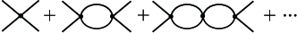
Figure 1: Sum of the infinite set of diagrams that contributes to the meson-meson scattering amplitude (1).

The loop function $G(s)$ is expanded as a Taylor series about $\mu^{2}$

$$G(s)=G(\mu^{2})+(s-\mu^{2})G^{\prime}(\mu^{2})+(s-\mu^{2})G_{h}(s)$$

where $G_{h}(s)$ contains higher order terms and vanishes at $\mu^{2}$, $G_{h}(\mu^{2})=0$. The scattering amplitude is then given by

$$t(s)=g^{2}(s)\frac{1}{s-\mu^{2}},$$ (3)

where the coupling $g(s)$ of the bound state to the two mesons is defined by

$$g^{2}(s)=-\frac{1}{G^{\prime}(\mu^{2})+G_{h}(s)}\ .$$ (4)

Hereafter we refer to a model which generates such a composite state as a composite model.

Now, we consider a Yukawa model which has only a three-point interaction of an elementary particle with the two mesons. With a bare coupling constant $g_{0}$, the full scattering amplitude as shown in Fig. 2 is given by

$$t_{Y}(s)=g_{0}^{2}\Delta(s)\ ,$$ (5)

where $\Delta(s)$ is the dressed propagator given by

$$\Delta(s)=\frac{1}{s-M_{0}^{2}-g_{0}^{2}G(s)}\ .$$ (6)

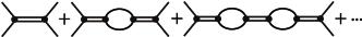
Figure 2: Scattering amplitude in the Yukawa model.

Here we have assumed that the loop function $G(s)$ in the Yukawa model is the same as that in the composite model. If the amplitudes $t_{Y}$ of Eq. (5) in the Yukawa model and $t$ of Eq. (3) in the composite model are equal, $t_{Y}$ should have a pole at the same position $\mu^{2}$ as $t$. By expanding the loop function $G(s)$ again, we obtain

$$t_{Y}=\frac{g_{0}^{2}}{1-g_{0}^{2}(G^{\prime}(\mu^{2})+G_{h}(s))}\frac{1}{s-\mu^{2}}\ ,$$ (7)

from which the renormalized coupling $g_{R}$ at the pole position is defined by

$$g_{R}^{2}=Zg_{0}^{2}\ .$$ (8)

Here $Z$ is the wave function renormalization constant defined by

$$Z = \left(1-g_{0}^{2}G^{\prime}(\mu^{2})\right)^{-1}$$ (9)

$$= 1+g_{R}^{2}G^{\prime}(\mu^{2})\ .$$ (10)

Equivalence of $t$ and $t_{Y}$ requires that the renormalized coupling $g_{R}^{2}$ at the pole position is equal to $g^{2}$ in Eq. (4)

$$g_{R}^{2}(\mu^{2}){=g^{2}(\mu^{2})}=-\frac{1}{G^{\prime}(\mu^{2})}\ .$$ (11)

With Eqs. (10) and (11), one can conclude that the wave function renormalization constant for the bound state is zero. It implies that the bare, unrenormalized, field $\phi=Z^{1/2}\phi_{R}$ in the Yukawa model vanishes for the composite boson. This is the content of the so-called “compositeness condition $Z=0$” from the field theoretical point of view discussed in Ref. Lurie and Macfarlane (1964); *Lurie:book.

The relation (10) between the wave function renormalization constant $Z$ and the renormalized coupling $g_{R}$ is employed also in the estimation of the compositeness for the deuteron system in Ref. Weinberg (1965). There the (renormalized) coupling $g_{R}$ is estimated by experimental data of the low-energy $p$-$n$ scattering. In Ref. Weinberg (1965), the $p$-$n$-$d$ coupling does not have an energy-dependence, and the non-relativistic form of the loop function is employed. The estimated $Z$ in Ref. Weinberg (1965) corresponds to the wave function renormalization constant for the fictitious elementary particle (deuteron) in the Yukawa model (5) with the constant coupling.

The above discussion cannot be directly applied to a resonant state. One way to allow an $s$-wave resonance is to take the interaction $v$ energy dependent. It turns out that the scattering amplitude with an energy-dependent $v(s)$ cannot be replaced by the Yukawa amplitude $t_{Y}$ in Eq. (5) with the energy-independent coupling $g_{0}$. Instead, we introduce an equivalent Yukawa model to a composite model with the energy-dependent interaction $v(s)$ where the both models give completely the same scattering amplitude, and discuss the wave function renormalization constant.

II.2 Energy dependent interaction; Weinberg-Tomozawa type

Let us consider a composite model with an energy-dependent interaction $v(s)$ which generates dynamically an $s$-wave composite state. In this section, we consider a specific form for the energy-dependent interaction, that is the Weinberg-Tomozawa (WT) type, and then later we generalize it in Sec. II.3. The WT interaction takes the following form,

$$v(s)=-\frac{1}{f^{2}}(s-m^{2})\ ,$$ (12)

where $f$ and $m$ are constants having dimensions of mass. This is a contact interaction as shown in the first diagram in Fig. 1.

By summing up the infinite set of diagrams as shown in Fig. 1, we obtain the scattering amplitude $T$ as

$$T(s)=\frac{1}{v(s)^{-1}-G(s)}\ ,$$ (13)

where the on-shell factorization is employed Oller and Oset (1997). Here $G(s)$ is the loop function in Eq. (2) which is regularized appropriately. If the potential $v(s)$ is attractive enough, the amplitude develops a pole at mass $\mu$ satisfying

$$v(\mu^{2})^{-1}-G(\mu^{2})=0\ ,$$ (14)

with the regularized $G$. The pole corresponds to a bound state if it appears below the threshold, or to a resonant state if above the threshold. The resonant state is a consequence of the energy dependent interaction $v(s)$, while a constant interaction $v$ can generate only a bound state.

Before constructing a Yukawa model giving the scattering amplitude which is exactly equivalent to $T(s)$ in Eq. (13), we attempt to shift the denominator of Eq. (13) by a constant $\delta(>0)$ as

$$T_{\delta}(s)=\frac{1}{v(s)^{-1}-G(s)+\delta}\ ,$$ (15)

and later let $\delta$ be zero again. It is clear that the shifted amplitude $T_{\delta}(s)$ smoothly reduces to the original $T(s)$ in the limit $\delta\rightarrow 0$ as

$$\lim_{\delta\rightarrow 0}T_{\delta}(s)=T(s)\ .$$

The shifted amplitude $T_{\delta}(s)$ has a pole at $\mu_{\delta}^{2}$ satisfying

$$v(\mu^{2}_{\delta})^{-1}-G(\mu^{2}_{\delta})+\delta=0\ ,$$ (16)

which also reduces to $\mu^{2}$ in the limit $\delta\rightarrow 0$ as

$$\lim_{\delta\rightarrow 0}\mu_{\delta}^{2}=\mu^{2}\ .$$

The inverse of the interaction kernel $v(s)^{-1}$ is expanded as a Taylor series about the pole $\mu_{\delta}^{2}$ as

$$v(s)^{-1} = -\frac{f^{2}}{s-m^{2}}$$

$$= -\frac{f^{2}}{\mu_{\delta}^{2}-m^{2}}+\frac{f^{2}(s-\mu_{\delta}^{2})}{(\mu_{\delta}^{2}-m^{2})^{2}}+(s-\mu_{\delta}^{2})v_{h}(s)$$

where $v_{h}(s)$ contains higher order terms and becomes zero at $s=\mu_{\delta}^{2}$. Similarly the function $G(s)$ is expanded about $\mu_{\delta}^{2}$ as

$$G(s)=G(\mu_{\delta}^{2})+(s-\mu_{\delta}^{2})G^{\prime}(\mu_{\delta}^{2})+(s-\mu_{\delta}^{2})G_{h}(s)\ .$$ (18)

By using Eqs. (16), (LABEL:eq:vinv) and (18) the amplitude $T_{\delta}(s)$ can be equivalently written as

$$T_{\delta}(s)=g_{R}^{2}(s)\frac{1}{s-\mu_{\delta}^{2}}\ ,$$ (19)

where

$$g^{2}_{R}(s)=\left(\frac{f^{2}}{(\mu_{\delta}^{2}-m^{2})^{2}}+v_{h}(s)-G^{\prime}(\mu^{2}_{\delta})-G_{h}(s)\right)^{-1}$$ (20)

is interpreted as an effective coupling of the composite state to the two mesons. At the pole position $s=\mu_{\delta}^{2}$ it is given by,

$$g^{2}_{R}(\mu_{\delta}^{2})=\left(\frac{f^{2}}{(\mu_{\delta}^{2}-m^{2})^{2}}-G^{\prime}(\mu^{2}_{\delta})\right)^{-1}\ .$$ (21)

Now let us construct a Yukawa model giving exactly the same scattering amplitude in the composite model in Eq. (13). The prescription is similar to the one developed in Ref. Hyodo et al. (2008) in which the CDD-pole component is discussed. Let us define a function $V_{Y}(s)$ by

$$V_{Y}(s)^{-1}\equiv v(s)^{-1}+\delta$$ (22)

so that

$$V_{Y}(s)=\frac{\frac{1}{\delta}(s-m^{2})}{s-m^{2}-\frac{f^{2}}{\delta}}.$$ (23)

By defining $m_{\text{fic}}^{2}$ by

$$m_{\text{fic}}^{2}\equiv\frac{f^{2}}{\delta}+m^{2}\$$ (24)

and eliminating $\delta$, we find an expression

$$V_{Y}(s)=\frac{1}{f^{2}}(m_{\text{fic}}^{2}-m^{2})(s-m^{2})\frac{1}{s-m_{\text{fic}}^{2}}\ .$$ (25)

Here $m_{\text{fic}}$ can be interpreted as the bare mass of the fictitious elementary particle. The function in front of the propagator is interpreted as the bare coupling of the fictitious particle to the two mesons defined as

$$g_{0}^{2}(s;m_{\text{fic}})\equiv\frac{1}{f^{2}}(m_{\text{fic}}^{2}-m^{2})(s-m^{2})\ .$$ (26)

With these interpretations we can regard $V_{Y}(s)$ as a Yukawa pole term with the energy-dependent coupling $g_{0}(s;m_{\text{fic}})$. We note that, in Ref. Hyodo et al. (2008), an additional CDD-pole term is defined by subtracting the WT term $v(s)$ from $V_{Y}(s)$ in Eq. (25). Here the trick in our study is to regard the whole of $V_{Y}(s)$ of Eq. (25) as the Yukawa pole term, and the constant $\delta$ is treated just as a parameter.

Now we shall see that the scattering amplitude of the composite model in Eq. (13) can be generated by the Yukawa model as shown in Fig. 2 as

$$T_{Y}(s)=g_{0}^{2}(s;m_{\text{fic}}){\Delta(s)}\ ,$$ (27)

where the dressed propagator $\Delta(s)$ for the fictitious elementary particle is given by

$$\Delta(s)=\frac{1}{s-m_{\text{fic}}^{2}-g_{0}^{2}(s;m_{\text{fic}})G(s)}\ .$$ (28)

The scattering amplitude (27) is identical with the shifted amplitude $T_{\delta}(s)$ in Eq. (15) and then reduces to $T(s)$ in Eq. (13) in the limit $\delta\rightarrow 0$,

$$\lim_{\delta\rightarrow 0}T_{Y}(s)=T(s)\ .$$

In this manner, the Yukawa pole term $V_{Y}(s)$ of Eq. (25) in the Yukawa model is equivalent to the four-point WT type interaction of Eq. (12) in the composite model.

Since we have defined the dressed propagator $\Delta(s)$ of the fictitious elementary Yukawa particle as in Eq. (28), we can evaluate the wave function renormalization constant for it. We expand the self-energy defined by

$$\Pi(s;m_{\text{fic}})\equiv g_{0}^{2}(s;m_{\text{fic}}^{2})G(s)$$ (29)

as a Taylor series about the pole $\mu^{2}_{\delta}$ as

$$\Pi(s;m_{\text{fic}}) = \Pi(\mu^{2}_{\delta};m_{\text{fic}})+(s-\mu^{2}_{\delta})\Pi^{\prime}(\mu^{2}_{\delta};m_{\text{fic}})$$ (30)

$$+ (s-\mu^{2}_{\delta})\Pi_{h}(s)$$

where again $\Pi_{h}$ contains higher order terms and becomes zero at $s=\mu^{2}_{\delta}$. The dressed propagator $\Delta(s)$ in Eq. (28) has the pole at

$$m_{\text{fic}}^{2}+\Pi(\mu^{2}_{\delta};m_{\text{fic}})$$

$$= m_{\text{fic}}^{2}+\frac{1}{f^{2}}(m_{\text{fic}}^{2}-m^{2})(\mu_{\delta}^{2}-m^{2})G(\mu_{\delta}^{2})$$

$$= \mu^{2}_{\delta}\ ,$$

which is the same as the pole position of $T_{\delta}(s)$. Here we have used Eqs. (16) and (24). The dressed propagator ${\Delta}(s)$ can be rewritten as,

$$\Delta{(s)}=\frac{1}{1-\Pi^{\prime}(\mu_{\delta};m_{\text{fic}})-\Pi_{h}(s)}\frac{1}{s-\mu^{2}_{\delta}}\ ,$$

and the wave function renormalization constant for the fictitious particle is defined by

$$Z=\left(\left.1-\Pi^{\prime}(s;m_{\text{fic}})\right|_{s=\mu^{2}_{\delta}}\right)^{-1}\ .$$ (31)

The derivative of the self-energy $\Pi$ is obtained by

$$\left.\Pi^{\prime}(s;m_{\text{fic}})\right|_{s=\mu^{2}_{\delta}} = \frac{1}{f^{2}}(m_{\text{fic}}^{2}-m^{2})G(\mu^{2}_{\delta})$$

$$+ \frac{1}{f^{2}}(m_{\text{fic}}^{2}-m^{2})(\mu^{2}_{\delta}-m^{2})G^{\prime}(\mu^{2}_{\delta})$$

$$= \frac{\mu^{2}_{\delta}-m_{\text{fic}}^{2}}{\mu_{\delta}^{2}-m^{2}}+{g_{0}^{2}(\mu_{\delta}^{2};m_{\text{fic}}^{2})}G^{\prime}(\mu^{2}_{\delta})\ .$$

Note that we have the first term of Eq. (LABEL:eq:Pi') in addition to the derivative of the loop function $G$ as in Eq. (9). This is the consequence of the energy dependence of the bare coupling $g_{0}^{2}$ and is non-negligible in the present analysis. The inverse of the wave function renormalization constant $Z^{-1}$ is obtained by

$$Z^{-1} = \frac{(\mu^{2}_{\delta}-m^{2})(m_{\text{fic}}^{2}-m^{2})}{f^{2}}\left\{\frac{f^{2}}{(\mu^{2}_{\delta}-m^{2})^{2}}-G^{\prime}(\mu_{\delta}^{2})\right\}$$ (34)

$$= g_{0}^{2}(\mu_{\delta}^{2};m_{\text{fic}})\frac{1}{g_{R}^{2}(\mu_{\delta}^{2})}\ ,$$

where in the last line we use Eq. (21) and (26).

The Yukawa model with the fictitious elementary particle in the limit $\delta\rightarrow 0$ is identical with the composite model in the sense that both models give the same scattering amplitude in the whole energy range. Since the loop function $G(s)$ has been regularized, the renormalized coupling $g_{R}$ remains finite in the limit $\delta\rightarrow 0$, except for a singular point $G^{\prime}(s)$ at the threshold. (We will return to this point later in Sec. IV.) Because the mass of the fictitious particle $m_{\text{fic}}$ in Eq. (24) diverges in the limit $\delta\rightarrow 0$, the bare coupling $g_{0}$ also does;

$$\lim_{\delta\rightarrow 0}m_{\text{fic}}^{2}=\infty\ ,$$

$$\lim_{\delta\rightarrow 0}g_{0}^{2}=\infty\ .$$

As a consequence, the wave function renormalization constant $Z$ must be zero in the limit $\delta\rightarrow 0$ as

$$\lim_{\delta\rightarrow 0}Z=0\ .$$

This means that any composite state dynamically generated by the WT type interaction can be represented by a fictitious elementary Yukawa particle with $Z=0$ whose bare field $\phi=Z^{1/2}\phi_{R}$ vanishes. This conclusion does not depend on cut-off scale.

We stress here that the condition $Z=0$ for the composite state is not due to the divergence of the loop function $G$, nor $G^{\prime}$, but those of the self-energy $\Pi$ and $\Pi^{\prime}$ as implied in Eq. (31). The underlying mechanism of $Z=0$ is that the bare coupling $g_{0}$ in the Yukawa model is proportional to the bare mass of the fictitious particle $m_{\text{fic}}$, which diverges to be consistent with the composite model. In the present Yukawa model, the fictitious elementary particle with the infinite mass becomes the physical resonant state by the one-loop correction with the infinite Yukawa coupling $g_{0}$ and the finite (regularized) loop function $G(s)$.

Here, we would like to note that our observation of $Z=0$ differs from the argument in Ref. Hyodo et al. (2012), where the wave function renormalization constant for a composite state generated by the WT interaction is not zero. This difference comes from the different definitions of the corresponding Yukawa models. The wave function renormalization constant $Z$ defined in Ref. Hyodo et al. (2012) is for a Yukawa particle with a constant coupling as defined in Eq. (10) Lurie and Macfarlane (1964); *Lurie:book; Weinberg (1965). In contrast, here we have shown that it is possible to construct the Yukawa model which is completely equivalent with the composite model with the energy dependent WT interaction by allowing an energy-dependent coupling $g_{0}(s)$ (26).

To see a role of the energy-dependence of $g_{0}$ more clearly, we rewrite $Z$ in the energy-dependent Yukawa model in Eq. (31) as,

$$Z=\frac{1}{1-\frac{\mu^{2}_{\delta}-m_{\text{fic}}^{2}}{\mu^{2}_{\delta}-m^{2}}}\left(1+g_{R}^{2}(\mu^{2}_{\delta})G^{\prime}(\mu^{2}_{\delta})\right)$$ (35)

where we have used Eqs. (31), (LABEL:eq:Pi') and (34). By comparing Eqs. (10) and (35), we can see that the difference is the term $(\mu^{2}_{\delta}-m_{\text{fic}}^{2})/(\mu^{2}_{\delta}-m^{2})$, which comes from the first term of Eq. (LABEL:eq:Pi') due to the energy dependence of the Yukawa coupling. Equation (35) can be further rewritten as

$$Z = \frac{\mu^{2}_{\delta}-m^{2}}{m_{\text{fic}}^{2}-m^{2}}\left(1+g_{R}^{2}(\mu^{2}_{\delta})G^{\prime}(\mu^{2}_{\delta})\right)$$

$$= \frac{\delta}{f^{2}}(\mu_{\delta}^{2}-m^{2})\left(1+g_{R}^{2}(\mu^{2}_{\delta})G^{\prime}(\mu^{2}_{\delta})\right)$$

which becomes zero with $m_{\text{fic}}^{2}\rightarrow\infty$ or $\delta\rightarrow 0$. Unlike the case of the constant interaction $v$, with the WT interaction $v(s)$ the renormalized coupling $g_{R}^{2}$ is not equal to $-1/G^{\prime}$. Instead, the additional term $(\mu^{2}_{\delta}-m_{\text{fic}}^{2})/(\mu^{2}_{\delta}-m^{2})$ owing to the energy dependence of the Yukawa model plays the crucial role to achieve $Z=0$.

II.3 Energy dependent interaction; general form

In the previous section, we have considered the WT type interaction to generate a composite state. Here we generalize the discussion to a general form of the interaction kernel and discuss the requirement to obtain $Z=0$. Let us assume that the interaction kernel $v(s)$ has an energy-dependence and is attractive enough to generate a resonant or bound state. We again start from the shifted amplitude $T_{\delta}(s)=(v^{-1}(s)-G(s)+\delta)^{-1}$ by a constant $\delta(>0)$. Following the same procedure in Eqs. (LABEL:eq:vinv)–(21), the (renormalized) coupling $g_{R}$ is obtained at $\mu_{\delta}^{2}$ as

$$g_{R}^{2}(\mu_{\delta}^{2})=\frac{v(\mu_{\delta}^{2})}{v^{\prime}(\mu_{\delta}^{2})(\delta-G(\mu_{\delta}^{2}))-v(\mu_{\delta}^{2})G^{\prime}(\mu^{2}_{\delta})}\ .$$ (36)

The equivalent Yukawa pole term is constructed from

$$V_{Y}(s)=\frac{1}{v(s)^{-1}+\delta}=\frac{v(s)}{1+v(s)\delta}\ .$$ (37)

For an attractive $v(s)$, $V_{Y}(s)$ has a pole for a positive $\delta$ at the energy satisfying

$$v(s)=-\frac{1}{\delta}\ .$$ (38)

The mass of the fictitious elementary particle $m_{\text{fic}}$ is defined by the solution of Eq. (38). We expand $v(s)$ about $m_{\text{fic}}^{2}$ as

$$v(s)=v(m_{\text{fic}}^{2})+(s-m_{\text{fic}}^{2})h(s;m_{\text{fic}}^{2})$$

and rewrite $V_{Y}$ as an explicit pole term as

$$V_{Y}(s)=\frac{1}{\delta}\frac{v(s)}{h(s;m_{\text{fic}}^{2})}\frac{1}{s-m_{\text{fic}}^{2}}\ .$$ (39)

By defining the bare coupling $g_{0}^{2}$ as

$$g_{0}^{2}(s;m_{\text{fic}})=\frac{1}{\delta}\frac{v(s)}{h(s;m_{\text{fic}}^{2})}\ ,$$ (40)

the scattering amplitude in the Yukawa model is expressed as

$$T_{Y}(s)=g_{0}^{2}(s;m_{\text{fic}}^{2})\Delta(s)\ ,$$

where the dressed propagator of the fictitious particle is given by

$$\Delta(s)=\frac{1}{s-m_{\text{fic}}^{2}-g_{0}^{2}(s;m_{\text{fic}}^{2})G(s)}\ .$$

Since the propagator $\Delta(s)$ has the pole at $\mu_{\delta}^{2}$ satisfying

$$m_{\text{fic}}^{2}+g_{0}^{2}(\mu_{\delta}^{2};m_{\text{fic}})G(\mu_{\delta}^{2})=\mu_{\delta}^{2},$$

the bare coupling $g_{0}^{2}$ in Eq. (40) can be expressed at the pole position as

$$g_{0}^{2}(\mu_{\delta}^{2};m_{\text{fic}})=\frac{\mu_{\delta}^{2}-m_{\text{fic}}^{2}}{G(\mu_{\delta}^{2})}$$ (41)

We follow Eqs. (30)–(34) and obtain

$$Z^{-1} = \frac{\mu^{2}_{\delta}-m_{\text{fic}}^{2}}{G(\mu_{\delta}^{2})v(\mu_{\delta}^{2})}\left\{v^{\prime}(\mu_{\delta}^{2})(\delta-G(\mu_{\delta}^{2}))-v(\mu_{\delta}^{2})G^{\prime}(\mu^{2})\right\}$$ (42)

$$= g_{0}^{2}(\mu_{\delta}^{2};m_{\text{fic}})\frac{1}{g_{R}^{2}(\mu^{2}_{\delta})}\ .$$

The renormalized coupling $g_{R}^{2}$ is finite in the limit $\delta\rightarrow 0$ with the regularized $G(s)$ and $G^{\prime}(s)$. The requirement to obtain $Z=0$ is again that $g_{0}^{2}$ diverges with $\delta\rightarrow 0$, and then $m_{\text{fic}}^{2}$ diverges as the solution of Eq. (38).

Now we observe from Eq. (38) that $|v(s)|$ diverges at $s=m_{\text{fic}}^{2}$ $(\delta\rightarrow 0)$. As shown in Fig. 3(a) (red solid line), the WT interaction in Eq. (12) diverges for large $s$, then $m_{\text{fic}}^{2}$ is infinite, and therefore the wave function renormalization constant is zero $Z=0$. In the light of these discussions, we can expect that an attractive interaction with a simple polynomial function of $\sqrt{s}$ which negatively diverges for large $s$ gives $Z=0$.

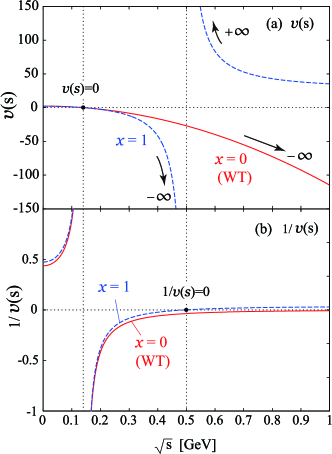
Figure 3: (color online) (a) Interaction kernel $v(s)$ in Eq. (45) and (b) its inverse $v(s)^{-1}$, with $x=0$ (the WT term) denoted by the red solid line and $x=1$ (WT + pole) by the blue dashed line, as functions of $\sqrt{s}$. The parameters are set to be $m=140$ MeV, $M_{0}=500$ MeV, $f=92.4$ MeV. The arrows in the figure indicate the divergent behaviors of the kernels.

II.4 Energy independent interaction

Now, we shall revisit the case of the constant interaction

$${v(s)=-c\ (c:\text{positive constant})}$$ (43)

discussed in Sec. II.1, by employing the above method to make the mechanism of $Z=0$ clearer. To find an equivalent Yukawa model, we introduce an $s$-dependent $\delta$-term as

$$T_{\delta}(s) = \frac{1}{-c+s\delta-G(s)}$$ (44)

$$= \frac{\frac{1}{\delta}}{s-\frac{1}{c\delta}-\frac{1}{\delta}G(s)}\ .$$

The equivalent Yukawa pole term is then defined in the same way as before as

$$V_{Y}(s)=g_{0}^{2}\frac{1}{s-m_{\text{fic}}^{2}}\ ,$$

where $m_{\text{fic}}^{2}$ and $g_{0}^{2}$ are defined as

$$m_{\text{fic}}^{2}\equiv\frac{1}{c\delta},\ \ \ g_{0}^{2}\equiv\frac{1}{\delta}=cm_{\text{fic}}^{2}\ \ .$$

We find again that the bare coupling constant of the Yukawa model is proportional to the mass of the fictitious elementary particle $m_{\text{fic}}$ which diverges in the limit $\delta\rightarrow 0$

$$\lim_{\delta\rightarrow 0}m_{\text{fic}}^{2}=\infty\ ,\lim_{\delta\rightarrow 0}g_{0}^{2}=\infty\ ,$$

and therefore that the wave function renormalization constant becomes zero $Z=0$ for bound states. By employing the above prescription we find that the mechanisms of $Z=0$ are the same for both the energy-dependent and energy-independent interactions in the composite model, where the bare mass of the fictitious elementary particle should be infinite. We can see clearly again that $Z=0$ is not a consequence of a divergence of the loop function $G$, nor $G^{\prime}$. This discussion also helps us to distinguish two different mechanisms of $Z=0$ later in Sec. IV.

Here in this section, we have introduced the equivalent elementary Yukawa model by introducing a constant $\delta$ or an $s$-dependent $\delta$-term and by taking subsequently the limit $\delta\rightarrow 0$. In the following section, we will also show that the constant shift in $v(s)^{-1}$ causes a divergence in the interaction $v(s)$ which means a presence of the explicit (elementary) pole term in the interaction $v(s)$. It will turn out that the above procedure is closely related to the regularization scale in the loop function $G$.

III Multiple interpretations of physical states

III.1 Cut-off dependence for one physical state

In this section we would like to discuss an arbitrariness of $Z$ which leads to multiple interpretations of physical states. To this end, we consider a composite model with an explicit pole term in addition to the WT interaction such as

$$v(s)=-\frac{1}{f^{2}}(s-m^{2})+\frac{x}{f^{2}}(s-m^{2})^{2}\frac{1}{s-M_{0}^{2}}\ ,$$ (45)

where $x$ is a parameter and $M_{0}$ the bare mass of an elementary particle. This kind of interaction is found in the sigma model in the nonlinear representation Oller and Oset (1997); Hyodo et al. (2010); Nagahiro and Hosaka (2013); Donoghue et al. (1992). In general, if the first WT interaction alone can generate a state and the second pole term introduces an additional degrees of freedom, the system has two physical poles Nagahiro et al. (2011). They are described as superpositions of the two basis states; the composite state developed by the WT term and the elementary particle in the pole term.

Indeed, by employing the interaction kernel $v(s)$ in Eq. (45), we find two physical poles with the coefficient $0<x<1$. However one of them disappears exactly at $x=1$ with

$$v(s)=-\frac{1}{f^{2}}(s-m^{2})+\frac{1}{f^{2}}(s-m^{2})^{2}\frac{1}{s-M_{0}^{2}}\ .$$ (46)

The sigma ($\sigma(500)$) resonance in the sigma model corresponds to this case as discussed in detail in Ref. Nagahiro and Hosaka (2013).

Let us first study the case $x=1$ which generates only one physical pole. In this case the equivalent Yukawa pole term can be obtained by rewriting Eq. (46) as,

$$v(s)=V_{Y}(s)=\frac{1}{f^{2}}(s-m^{2})(M_{0}^{2}-m^{2})\frac{1}{s-M_{0}^{2}}\ .$$ (47)

Alternatively, the bare mass of the “fictitious particle” $m_{\text{fic}}^{2}$ is given by a solution of Eq. (38) as

$$m_{\text{fic}}^{2}=\frac{m^{2}(M_{0}^{2}-m^{2})\delta+f^{2}M_{0}^{2}}{(M_{0}^{2}-m^{2})\delta+f^{2}}\ ,$$

which reduces to $M_{0}^{2}$ in the limit $\delta\rightarrow 0$ showing that the equivalent Yukawa pole term (25) is again given by Eq. (47). We find that the bare coupling $g_{0}^{2}=(s-m^{2})(M_{0}^{2}-m^{2})/f^{2}$ is finite, and therefore the wave function renormalization constant $Z$ is non-zero. This result is natural; if there is an explicit pole term as in Eq. (46), $Z$ is finite. We can also see that a different bare mass $M_{0}$ of the explicit pole term in Eq. (46) leads to a different value of $Z$.

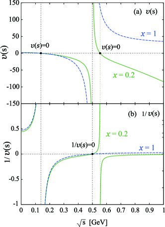
Figure 4: (color online) (a) Interaction kernel $v(s)$ in Eq. (45) and (b) its inverse $v(s)^{-1}$ with $x=0.2$ denoted by the green solid line and with $x=1$ by the blue dashed line as functions of $\sqrt{s}$. The parameters are set to be $m=140$ MeV, $M_{0}=500$ MeV, $f=92.4$ MeV.

Now, let us look at the above problem in a different way by comparing the two cases of $x=1$ and of $x=0$. As shown in Fig. 3, although the shapes of $v(s)$ with ($x=1$) and without ($x=0$) the pole term are quite different, their inverses $v(s)^{-1}$ are quite similar. Indeed, they are different only by a constant $a$,

$$v_{x=1}(s)^{-1}=v_{x=0}(s)^{-1}+a\ ,$$ (48)

which can be absorbed into the loop function $G$ in the scattering amplitude as

$$T(s)^{-1} = v_{x=1}(s)^{-1}-G(s)$$ (49)

$$= v_{x=0}(s)^{-1}+a-G(s)$$ (50)

$$= v_{x=0}(s)^{-1}-\tilde{G}(s)$$ (51)

where $\tilde{G}(s)\equiv G(s)-a$. This can be done by changing the subtraction constant in the dimensional regularization which is equivalent to changing $\Lambda$ in the cut-off regularization schemes. Physically, the change in $G$ corresponds to a different choice of the dynamical composite model. Since the form of the scattering amplitude (51) is the same as discussed in Sec. II.2, we can conclude that the wave function renormalization constant $Z$ is zero for this system. The above step is nothing but the one developed in Ref. Hyodo et al. (2008), but we follow it in the opposite way.

Now, we find that there are two different interpretations for the physical pole:

• The physical pole originates in the elementary Yukawa particle with a finite bare mass $M_{0}$ as in Eq. (47), which acquires the one loop correction, leading to $Z\neq 0$.

• The physical pole originates in the WT term in Eq. (46) with $Z=0$. The pole term in Eq. (46) is absorbed as a counter term into the loop function.

The above examples show that there is an arbitrariness in the interpretation. We can express the physical state as a pure composite state with $Z=0$ as well as an elementary particle with $Z\neq 0$. In Eqs. (49)–(51), we have seen that the parameter $a$ can be combined either with $v^{-1}$ or with $G(\tilde{G})$. Depending on these two schemes, $Z$ can take any value, while the scattering amplitude $T$ and so physical observables are invariant. In other words, $Z$ cannot be determined from experiments in a model independent manner.

If we can fix $G$ by using some external condition, we may be able to partly avoid such arbitrariness. This can be done, for instance, by introducing a cut-off parameter for $G$, keeping track of its origin, for instance, to the intrinsic size of the constituents.

III.2 Two physical states : two-level problem

So far, we have studied the case of $x=1$. For $0<x<1$, a different feature appears; the interaction (45) can generate two physical poles rather than one. As shown in Fig. 4, although the interaction kernel $v(s)$ with, say $x=0.2$, shows similar behavior with $x=1$, the shape of $v(s)^{-1}$ is quite different. For $x<1$, an additional divergent point appears in $v(s)^{-1}$ which produces the second physical pole satisfying $v^{-1}-G=0$. The difference between $v(s)^{-1}$ with $x=0$ and $x=0.2$, as can be seen in Fig. 4, cannot be absorbed by a constant, nor by any smooth function. Therefore, the interpretation 2) in the previous subsection cannot be applied.

Furthermore, the interpretation 1) also cannot be directly applied. Since we have two physical states, we cannot express the scattering amplitude by using a single Yukawa pole term $V_{Y}(s)$. In fact we have two solutions of Eq. (38) for $m_{\text{fic}}$ as

$$m_{\text{fic}}^{2}=\begin{cases}M_{0}^{2}+{\cal O}(\delta)\xrightarrow{\delta\rightarrow 0}M_{0}^{2}\\ {\cal O}(\frac{1}{\delta})\xrightarrow{\delta\rightarrow 0}\infty\end{cases}$$

indicating that there are two “seeds” for two physical states. The nature of the physical states is different from the previous ones, leading to the following interpretation;

• The physical poles are mixtures of the WT composite state generated by the first term in Eq. (46) and the elementary particle of the second term in Eq. (46).

The two physical states are described as superpositions of the two “seeds”, one is the elementary particle with the finite mass $M_{0}$ and the other is the fictitious elementary particle with infinite bare mass. This is schematically expressed as

$$|\text{pole-}a\rangle = c_{1}|m_{\text{fic}}\rangle+c_{2}|M_{0}\rangle$$

$$|\text{pole-}b\rangle = c_{3}|m_{\text{fic}}\rangle+c_{4}|M_{0}\rangle\ ,$$

which can be analyzed in terms of the two-level problem Nagahiro et al. (2011). The component $c_{i}$ is the wave function renormalization constant $\sqrt{Z}$ at each pole position pole-$a$ or pole-$b$ for each basis state .

We note once again that there is arbitrariness in $c_{i}$’s (or $Z$’s), depending on the choice of the basis states $|m\rangle$. For example, as done in Ref. Nagahiro et al. (2011), it is possible to first sum up only the WT interaction to obtain the WT composite state, and redefine the developed pole as “pure” composite state $|m_{WT}\rangle$. Then we mix it with the elementary particle, and discuss their mixing,

$$|\text{pole-}a\rangle = c_{1}^{\prime}|m_{WT}\rangle+c_{2}^{\prime}|M_{0}\rangle$$

$$|\text{pole-}b\rangle = c_{3}^{\prime}|m_{WT}\rangle+c_{4}^{\prime}|M_{0}\rangle\ .$$

Other definitions of the basis states are also possible. By choosing the basis states appropriately, we can discuss their mixing to understand the nature of the physical states Nagahiro et al. (2011); Nagahiro and Hosaka (2013).

III.3 Model dependence of $Z$ : demonstration in the sigma model

Finally in this section, we discuss further a model dependence of $Z$. In Sec. II, we have introduced the Yukawa model as

$$V_{Y}(s) = \frac{(s-m^{2})(m_{\text{fic}}^{2}-m^{2})}{f^{2}}\frac{1}{s-m_{\text{fic}}^{2}}$$ (52)

$$\equiv g_{0}^{2}(s)\frac{1}{s-m_{\text{fic}}^{2}}\ ,$$

which has only the three-point interaction and is equivalent to the composite model with the WT interaction. This expression can be further rewritten into two different forms as

$$V_{NL}(s) = -\frac{(s-m^{2})}{f^{2}}+\frac{(s-m^{2})^{2}}{f^{2}}\frac{1}{s-m_{\text{fic}}^{2}}$$ (53)

$$\equiv v_{WT}(s)+g_{NL}^{2}(s)\frac{1}{s-m_{\text{fic}}^{2}},$$

and

$$V_{L}(s) = \frac{(m_{\text{fic}}^{2}-m^{2})}{f^{2}}+\frac{(m_{\text{fic}}^{2}-m^{2})^{2}}{f^{2}}\frac{1}{s-m_{\text{fic}}^{2}}$$ (54)

$$\equiv v_{4}+g_{L}^{2}\frac{1}{s-m_{\text{fic}}^{2}}\ ,$$

which might define two different “models” (or more concretely different diagrams) as depicted Fig. 5. Here we refer to the second model as “nonlinear (NL) model” and the third as “linear (L) model” for sake of simplicity. The interaction $V_{NL}(s)$ in Eq. (53) consists of the WT term $v_{WT}(s)$ and the pole term with the energy-dependent bare coupling $g_{NL}(s)$. The interaction $V_{L}(s)$ in Eq. (54) has a repulsive four-point interaction $v_{4}$ and the pole term with the constant coupling $g_{L}$.

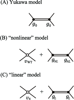
Figure 5: Tree amplitudes in (A) the Yukawa model in Eq. (52), (B) the “nonlinear” model in Eq. (53), and (C) the “linear” model in Eq. (54). The solid and open circles are for the three-point vertices and for the four-point interactions, respectively.

Although these interactions contain the same propagator $(s-m_{\text{fic}}^{2})^{-1}$ of a fictitious elementary particle and the resulting scattering amplitude are the same, the corresponding wave function renormalization constants for these fictitious particles are different.

For example, in the linear model the wave function renormalization constant $Z_{{L}}$ in the limit $\delta\rightarrow 0$ $(m_{\text{fic}}\rightarrow\infty)$ is not zero, while in the nonlinear or in the Yukawa model it is zero, $Z_{NL}=Z_{Y}=0$. In the linear model, the scattering amplitude is given by

$$T(s)=T_{4}(s)+{\tilde{g}_{L}}^{2}(s)\Delta_{L}(s)\ ,$$

where $T_{4}$ is defined by

$$T_{4}(s)=\frac{1}{v_{4}^{-1}-G(s)}\ ,$$

with the repulsive four-point interaction $v_{4}$ Weinberg (1963). The coupling ${\tilde{g}_{L}}$ contains vertex corrections due to the contact interaction $v_{4}$ as

$${\tilde{g}_{L}}(s)=\frac{g_{L}}{1-v_{4}G(s)}\ .$$

The dressed propagator $\Delta_{L}$ is given by

$$\Delta_{L}(s)=\frac{1}{s-m_{\text{fic}}^{2}-\Pi_{L}(s)}\ ,$$

with the self-energy

$$\Pi_{L}(s) = g_{L}^{2}\frac{G(s)}{1-v_{4}G(s)}$$ (55)

$$= \frac{(m_{\text{fic}}^{2}-m^{2})^{2}}{f^{2}}\frac{G(s)}{1-\frac{(m_{\text{fic}}^{2}-m^{2})}{f^{2}}G(s)}\ ,$$

Figure 6: Self-Energy for the fictitious particle in the linear and nonlinear models. The solid and open circles indicate the couplings in the same manner as in Fig. 5.

dipicted in Fig. 6. The wave function renormalization constant $Z_{L}$ for the elementary particle is defined by using the self-energy as,

$$Z_{L}=\left(1-\left.\Pi_{L}^{\prime}(s)\right|_{s=\mu_{\delta}^{2}}\right)^{-1}\ .$$

The derivative $\Pi_{L}^{\prime}$ is calculated as

$$\left.\Pi_{L}^{\prime}(s)\right|_{s=\mu^{2}_{\delta}}=\frac{1}{f^{2}}\frac{G^{\prime}(\mu_{\delta}^{2})}{\left(\frac{1}{m_{\text{fic}}^{2}-m^{2}}-\frac{1}{f^{2}}G(\mu_{\delta}^{2})\right)^{2}}$$ (56)

and in the limit $\delta\rightarrow 0$ it reduces to

$$\left.\Pi_{L}^{\prime}(s)\right|_{s=\mu^{2}_{\delta}}\xrightarrow[m_{\text{fic}}\rightarrow\infty]{\delta\rightarrow 0}f^{2}\frac{G^{\prime}(\mu^{2})}{G(\mu^{2})^{2}}\ .$$ (57)

If $G(s)$ and $G^{\prime}(s)$ are regularized in the same manner as in the previous section, this derivative takes a finite value and then $Z_{L}$ is not equal to zero even in the limit $\delta\rightarrow 0$.

In the nonlinear model the scattering amplitude and the dressed propagator can be derived in a similar manner. The self-energy $\Pi_{NL}$ is now given by

$$\Pi_{NL}(s)=\frac{(s-m^{2})^{2}}{f^{2}}\frac{G(s)}{1+\frac{(s-m^{2})}{f^{2}}G(s)}.$$ (58)

The derivative of the self-energy is obtained by

$$\left.\Pi_{NL}^{\prime}(s)\right|_{s=\mu^{2}_{\delta}} = \frac{2G(\mu_{\delta}^{2})}{\delta}+\frac{f^{2}G^{\prime}(\mu_{\delta}^{2})-G(\mu_{\delta}^{2})^{2}}{\delta^{2}}\ .$$ (59)

Obviously, this quantity diverges in the limit $\delta\rightarrow 0$ leading to $Z_{NL}\rightarrow 0$. In the nonlinear case $\lim_{\delta\rightarrow 0}Z_{NL}=0$ can be explained also by using the two-level problem as discussed in Ref. Nagahiro and Hosaka (2013).

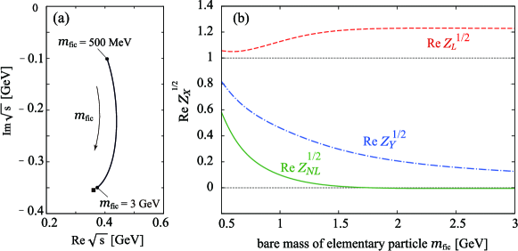
Figure 7: (color online) (a) Flow of the pole position of the sigma ($\sigma(500)$) resonance in the scattering amplitude obtaining by changing the bare mass of the elementary particle (sigma meson) from 0.5 GeV to 3 GeV. The solid square indicates the pole position in the limit $m_{\text{fic}}\rightarrow\infty$ Nagahiro and Hosaka (2013). (b) The real part of the wave function renormalization constants as functions of the bare mass of the elementary particle. The blue dash-dotted line is for the Yukawa model $(Z^{1/2}_{Y})$ with the interaction kernel (61), the green solid line for the nonlinear model $(Z^{1/2}_{NL})$ with (62), and the red dashed line for the linear model $(Z^{1/2}_{L})$ with (63).

Here we demonstrate the model dependence of $Z$ by using the sigma ($\sigma(500)$) meson in the sigma model. In Fig. 7, we show the wave function renormalization constant $Z$ for the three cases; with the Yukawa model ($Z_{Y}$), the nonlinear model ($Z_{NL}$) and the linear model ($Z_{L}$). The parameter $m$ is set to be the mass of the pion $m=m_{\pi}=138$ MeV, $f$ the pion decay constant $f=f_{\pi}=92.4$ MeV. The mass $m_{\text{fic}}$ corresponding to the bare mass of the elementary sigma meson is varied from 0.5 GeV to 3 GeV in the figure.

Here we note that for the isosinglet sigma meson we employ $3V_{X}(s)+V_{X}(t)+V_{X}(u)$ instead of $V_{X}(s)$ alone as the interaction kernel $(X=L$, $NL$, and $Y$). Although the inclusion of the $t$ and $u$ channels changes the expressions of the self-energies in Eqs. (29), (55) and (58), the conclusion about the fate of $Z_{X}$ for the large $m_{\text{fic}}$ limit is not affected. The $s$-wave tree amplitude for the $s$-wave resonance can be projected out by,

$$v(s)=\frac{1}{2}\int_{-1}^{1}dxT_{I=0}^{\rm tree}(s,t(x),u(x))P_{\ell=0}(x)$$ (60)

in the center of mass frame. The result of the projection is given by

$$v(s)_{Y} = g_{0}^{2}(s)\frac{1}{s-m_{\text{fic}}^{2}}+v^{\rm ex}_{Y}(s)$$ (61)

$$v(s)_{NL} = g_{NL}^{2}(s)\frac{1}{s-m_{\text{fic}}^{2}}+v^{\rm ex}_{NL}(s)+v^{\rm con}_{NL}(s)$$ (62)

$$v(s)_{L} = g_{L}^{2}\frac{1}{s-m_{\text{fic}}^{2}}+v^{\rm ex}_{L}(s)+v^{\rm con}_{L}(s)\ ,$$ (63)

where the bare couplings are now defined by

$$g_{0}^{2}(s) = \frac{3}{f^{2}}(s-m^{2})(m_{\text{fic}}^{2}-m^{2})$$ (64)

$$g_{NL}^{2}(s) = \frac{3}{f^{2}}(s-m^{2})^{2}$$ (65)

$$g_{L}^{2} = \frac{3}{f^{2}}(m_{\text{fic}}^{2}-m^{2})^{2}\ ,$$ (66)

and $v^{\rm ex}$ and $v^{\rm con}$ denote the ($s$-wave projected) $t$- and $u$-channel exchange and the contact terms, respectively. The concrete forms of (61)–(63) are summarized in Appendix A.

Since the three interaction kernels (61)–(63) are the same, the pole position of the physical $\sigma(500)$ resonance is the same for all cases, as shown in Fig. 7(a) Nagahiro and Hosaka (2013). However, the wave function renormalization constant $Z$ for the three cases are different as shown in Fig. 7(b). In the Yukawa model $Z_{Y}$ decreases and approaches zero as $m_{\text{fic}}$ is increased as discussed before. In the nonlinear model $Z_{NL}$ also decreases, and finally becomes zero in the limit $m_{\text{fic}}\rightarrow\infty$. In contrast, we find that the $Z_{L}$ of the linear model shows quite different behavior from the others. It remains finite even in the large $m_{\text{fic}}$ limit. These are consistent with the discussion in Eq. (56) and afterwards.

If we use the finite value of $Z_{L}$ in the linear model, we may interpret that the $\sigma(500)$ resonance has a large component of the elementary particle even if its bare mass is infinite. It does not conflict, however, to the other interpretations in the Yukawa and nonlinear models in which the elementary component is zero with the infinite bare mass, because each value of $Z$ indicates the probability of finding the elementary particle defined in each model: the elementary particles in different models are different.

IV Zero energy bound system

In this section we discuss the zero-energy bound state which also leads exactly to $Z=0$, but the underlying mechanism is very much different from what we have discussed so far. Let us recall that the mechanism of $Z=0$ discussed in the previous sections, where

$$g_{0}\rightarrow\infty\ (\text{then}\ m_{\text{fic}}\rightarrow\infty)\ \ \&\ \ g_{R}=\text{finite}$$ (67)

that is the bare mass of the fictitious particle must be infinite and far away from the energy region of interest. In contrast, there is another mechanism which also leads to $Z=0$ as

$$g_{0}=\text{finite}\ (\text{then}\ m_{\text{fic}}=\text{finite)}\ \&\ \ g_{R}=0\ .$$ (68)

This can be realized when the physical state appears at the threshold, namely zero-energy bound state. In fact, it was shown that the renormalized coupling constant $g_{R}^{2}$ is proportional to $\sqrt{|B|}$ for small $|B|$ Nambu and Sakurai (1961); Weinberg (1963),

$$g_{R}^{2}\propto\sqrt{|B|}\ ,$$

with the binding energy $B$. Consequently, $Z\rightarrow 0$ in the limit $B=0$. The behavior of $g_{R}$ at the threshold can be directly seen from Eq. (11) for the constant interaction case and from Eq. (21) for the WT interaction case, where we can see that $g_{R}=0$ due to the divergence of $G^{\prime}(s)$ at the threshold Hyodo et al. (2012).

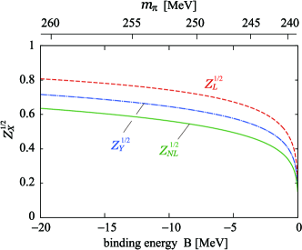
Figure 8: (color online) Wave function renormalization constants as functions of the binding energy. The blue dash-dotted line is for the Yukawa model ($Z_{Y}^{1/2}$) with the interaction kernel (61), the green solid line for the nonlinear model ($Z_{NL}^{1/2}$) with (62), and the red dashed line for the linear model ($Z_{L}^{1/2}$) with (63). The parameters are set to be $f=f_{\pi}=92.4$ and $m_{\text{fic}}=550$ MeV. The corresponding pion mass is indicated in the upper horizontal axis.

The important point here is that, the condition $Z=0$ for the zero-energy bound state has no relation to the bare mass of the elementary particle and does not mean its infinite value. As an example, in Fig. 8, we show the wave function renormalization constants for bound states in the three representations; the Yukawa ($Z_{Y}$), nonlinear ($Z_{NL}$), and linear ($Z_{L}$) models, as functions of the binding energy $B=\mu-2m_{\pi}$ where $\mu$ is the mass of the bound state. The models used here are the same as for Fig. 7 except the mass of the pion which is set lager to obtain a bound state with a finite $B$ below the threshold as indicated in Fig. 8. The bare mass of the elementary sigma meson is fixed to be $m_{\text{fic}}=550$ MeV. As discussed in Sec. III.3, the three wave function renormalization constants $Z_{X}$ are different from each other at finite binding energies $B$, but becomes zero at $B=0$ for all cases. However, $Z=0$ for the zero-energy bound state does not mean that the elementary particle is irrelevant in this system. Indeed, the energy (mass) of the physical state ($\sim 480$ MeV in this case) is determined by the bare mass of the elementary particle (550 MeV) together with the self-energy with finite $g_{0}$ and finite (regularized) $G$, which is independent from the divergence of $G^{\prime}$. Such a situation can arise in any composite state close to the threshold.

The “compositeness” or “elementarity” is often discussed without distinction between these two mechanisms (67) and (68). Although both gives the divergence of the derivative of the self-energy $\Pi^{\prime}=(g_{0}^{2}G)^{\prime}$, they should be discussed separately because the physical meanings are different. The so-called “elementarity” we would like to know is the former one, that is to say whether the energy (mass) of the elementary particle is far from the physical pole or not. The condition $Z=0$ for the zero-energy bound state does not exclude the existence of the elementary state close to the physical state.

V Summaries and discussions

We have discussed the “compositeness” or “elementarity” of composite states by means of the wave function renormalization constant $Z$. We have shown that $s$-wave scattering amplitudes and $s$-wave states generated dynamically by an energy-dependent or independent interaction can be equivalently represented by a Yukawa model with an energy-dependent or independent coupling and with the infinite bare mass of a fictitious elementary particle. Consequently, the wave function renormalization constant $Z$ for any composite state can be zero, which means that the corresponding bare elementary field $\phi=Z\phi_{R}$ vanishes. The idea can be equally applied to both resonant and bound states. Here the underlying mechanism of $Z=0$ is that the bare coupling and the bare mass of the corresponding Yukawa particle become infinite to be consistent with the composite state.

We have also discussed the case of the zero energy bound state, which also leads to $Z=0$. This is due to the divergence of the derivative of the loop function at the threshold, which should be distinguished from the above mentioned mechanism of the infinite bare mass of the fictitious elementary particle. The condition $Z=0$ for the zero-energy bound state does not exclude an elementary state near the physical state. Therefore we should be careful when we discuss the “elementarity” of barely bound systems.

The argument for the condition $Z=0$ with infinite bare mass corresponds to the assertion made by Weinberg in Ref. Weinberg (1963) that any physical state can be equivalently represented by a “quasi-particle” with infinite bare mass and hence with $Z=0$. To see what this statement means more clearly, let us consider hadron resonances in the chiral unitary approach Jido et al. (2003); Inoue et al. (2002). There, it is widely believed that $\Lambda(1405)$ is a good candidate of a composite state of weakly bound $\bar{K}N$ molecular state, while $N(1535)$ contains to a large extent non-composite component Hyodo et al. (2008). However, according to the assertion, both particles can be always made “composite” with zero elementarity, $Z=0$.

At first sight this statement sounds inconsistent. However, a solution can be given if we look at the setup of the chiral unitary approach which is defined together with a natural cut-off scale corresponding to the intrinsic size of the constituent hadrons. While the properties of $\Lambda(1405)$ can be well reproduced within the natural framework of the model, those of $N(1535)$ can be so when a cut-off scale is chosen at a value which is different from the natural value. As we will explain shortly, the use of the un-natural cut-off scale introduces a pole term in the interaction. We can then measure the compositeness by means of the elementary particle corresponding to the pole term, which leads to a finite value $Z\neq 0$. Without the pole term, as we have discussed so far, the renormalization constant $Z$ is equal to zero. In view of this, the value of the renormalization constant itself does not tell us the nature of the physical state.

Let us now look at the problem in a slightly different manner in terms of the physical observables, that is the scattering amplitude. Suppose we determine the cut-off value $\Lambda=\Lambda_{h}$ at the hadronic scale. However, the resulting scattering amplitude does not always reproduce observables. Then we attempt to change $\Lambda$ from $\Lambda_{h}$ to reproduce the observables. In the scattering amplitude, this amounts to the change in the loop function, $G(\Lambda_{h})\rightarrow G(\Lambda)$. The important point that should be emphasized here is that the difference $G(\Lambda)-G(\Lambda_{h})$ introduces the new pole interaction as, $v(s)\rightarrow\tilde{v}(s)=v(s)$ + pole term Hyodo et al. (2008). Then we can evaluate the renormalization constant $Z$ in terms of the elementary particle associated with the new pole term Nagahiro and Hosaka (2013). In this manner, the resulting $Z$ can take an arbitrary finite value. In other words, while the physical observable (amplitude) is invariant under the simultaneous changes in $G$ and the interaction $v$, the renormalization constant $Z$ cannot be determined from experiment in a model independent manner. This is an unavoidable feature because the renormalization constant $Z$ is not a physical observable.

To discuss the “elementarity”, we need to first specify a reasonable (or useful) framework for the dynamics of the system to make a proper description for hadrons. This is to a large extent a question of economization. The criterion for choosing a suitable model should be given by external conditions independently from the present discussions concerning the constant $Z$.

Appendix A tree amplitude for the $\pi\pi$ scattering

Here we show the concrete form of the interaction kernels in the $\pi\pi$ scattering amplitude in the sigma model Donoghue et al. (1992); Oller and Oset (1997); Hyodo et al. (2010); Nagahiro and Hosaka (2013). The tree amplitude for the isospin $I=0$ channel is determined in terms of a sigle function $V(s,t,u)$ as

$$T_{\rm tree}=3V(s,t,u)+V(t,s,u)+V(u,t,s).$$

The function $V(s,t,u)=V(s)$ is given by $V_{NL}$ in Eq. (53) in the nonlinear model Oller and Oset (1997); Hyodo et al. (2010), $V_{L}$ in Eq. (54) in the linear model Hyodo et al. (2010), and $V_{Y}(s)$ in Eq. (52) in the Yukawa model. The $s$-wave projection is performed by Eq. (60) and the results of the projection are given by,

$$v(s)_{Y} = g_{0}^{2}(s)\frac{1}{s-m_{\text{fic}}^{2}}-\frac{2}{f^{2}}(m_{\text{fic}}^{2}-m^{2})+\frac{1}{f^{2}}\frac{2(m^{2}-m_{\text{fic}}^{2})^{2}}{s-4m^{2}}\ln\left(\frac{m_{\text{fic}}^{2}}{m_{\text{fic}}^{2}-4m^{2}+s}\right)$$ (69)

$$v(s)_{NL} = g_{NL}^{2}(s)\frac{1}{s-m_{\text{fic}}^{2}}-\frac{1}{f^{2}}(2s-m^{2})+\frac{1}{f^{2}}\left\{-(s-2m_{\text{fic}}^{2})+\frac{2(m^{2}-m_{\text{fic}}^{2})^{2}}{s-4m^{2}}\ln\left(\frac{m_{\text{fic}}^{2}}{m_{\text{fic}}^{2}-4m^{2}+s}\right)\right\}$$ (70)

$$v(s)_{L} = g_{L}^{2}\frac{1}{s-m_{\text{fic}}^{2}}+\frac{5}{f^{2}}(m_{\text{fic}}^{2}-m^{2})+\frac{1}{f^{2}}\frac{2(m^{2}-m_{\text{fic}}^{2})^{2}}{s-4m^{2}}\ln\left(\frac{m_{\text{fic}}^{2}}{m_{\text{fic}}^{2}-4m^{2}+s}\right)$$ (71)

where the coupling $g_{0}^{2}$, $g_{NL}^{2}$, and $g_{L}^{2}$ are defined by Eqs. (64)–(66).

References

- Choi et al. (2003) S. K. Choi et al. (Belle), Phys. Rev. Lett. 91, 262001 (2003).
- Aubert et al. (2005) B. Aubert et al. (BABAR), Phys. Rev. D71, 071103 (2005).
- Choi et al. (2008) S. K. Choi et al. (BELLE), Phys. Rev. Lett. 100, 142001 (2008).
- Aaij et al. (2013) R. Aaij et al. (LHCb), Phys.Rev.Lett. 110, 222001 (2013).
- Oller et al. (1999) J. A. Oller, E. Oset, and J. R. Pelaez, Phys. Rev. D59, 074001 (1999).
- Baru et al. (2004) V. Baru, J. Haidenbauer, C. Hanhart, Y. Kalashnikova, and A. E. Kudryavtsev, Phys. Lett. B586, 53 (2004).
- Jido et al. (2003) D. Jido, J. A. Oller, E. Oset, A. Ramos, and U. G. Meissner, Nucl. Phys. A725, 181 (2003).
- Inoue et al. (2002) T. Inoue, E. Oset, and M. J. Vicente Vacas, Phys. Rev. C 65, 035204 (2002).
- Roca et al. (2005) L. Roca, E. Oset, and J. Singh, Phys. Rev. D72, 014002 (2005).
- Hyodo et al. (2008) T. Hyodo, D. Jido, and A. Hosaka, Phys. Rev. C78, 025203 (2008).
- Black et al. (2001) D. Black, A. H. Fariborz, S. Moussa, S. Nasri, and J. Schechter, Phys.Rev. D64, 014031 (2001), arXiv:hep-ph/0012278 [hep-ph] .
- Urban et al. (2002) M. Urban, M. Buballa, and J. Wambach, Nucl.Phys. A697, 338 (2002), arXiv:hep-ph/0102260 [hep-ph] .
- Fariborz et al. (2005) A. Fariborz, R. Jora, and J. Schechter, Int.J.Mod.Phys. A20, 6178 (2005).
- Fariborz et al. (2007) A. H. Fariborz, R. Jora, and J. Schechter, Phys.Rev. D76, 014011 (2007), arXiv:hep-ph/0612200 [hep-ph] .
- Parganlija et al. (2013) D. Parganlija, P. Kovacs, G. Wolf, F. Giacosa, and D. H. Rischke, Phys.Rev. D87, 014011 (2013), arXiv:1208.0585 [hep-ph] .
- Giacosa (2009) F. Giacosa, Phys.Rev. D80, 074028 (2009), arXiv:0903.4481 [hep-ph] .
- Weinberg (1963) S. Weinberg, Phys. Rev. 130, 776 (1963).
- Weinberg (1965) S. Weinberg, Phys. Rev. 137, B672 (1965).
- Lurie and Macfarlane (1964) D. Lurie and A. J. Macfarlane, Phys. Rev. 136, B816 (1964).
- Lurie (1968) D. Lurie, Particle and Fields (Interscience Publishers, New York, 1968).
- Hyodo et al. (2012) T. Hyodo, D. Jido, and A. Hosaka, Phys. Rev. C 85, 015201 (2012).
- Nagahiro et al. (2011) H. Nagahiro, K. Nawa, S. Ozaki, D. Jido, and A. Hosaka, Phys.Rev. D83, 111504 (2011).
- Nagahiro and Hosaka (2013) H. Nagahiro and A. Hosaka, Phys.Rev. C88, 055203 (2013).
- Oller and Oset (1997) J. Oller and E. Oset, Nucl.Phys. A620, 438 (1997).
- Hyodo et al. (2010) T. Hyodo, D. Jido, and T. Kunihiro, Nucl. Phys. A848, 341 (2010).
- Donoghue et al. (1992) J. F. Donoghue, E. Golowich, and B. R. Holstein, Dynamics of the Standard Model (Cambridge University Press, Cambridge, 1992).
- Nambu and Sakurai (1961) Y. Nambu and J. Sakurai, Phys.Rev.Lett. 6, 377 (1961).