Superradiance and enhanced luminescence from ensembles of a few self-assembled quantum dots

Abstract

We study theoretically the evolution of photoluminescence (PL) from homogeneous and inhomogeneous ensembles of a few coupled QDs. We discuss the relation between signals from a given QD ensemble under strong and weak excitation (full inversion and linear response regimes): A system homogeneous enough to manifest superradiant emission when strongly inverted shows a non-exponential decay of the PL signal under spatially coherent weak excitation. In an inhomogeneous ensemble the PL decay is always nearly exponential with a qualitatively different form of the time dependence in the two excitation regimes and with a higher rate under weak excitation.

I Introduction

Optical properties of arrays and ensembles of quantum dots (QDs) continue to attract attention both from the theoretical temnov05 ; temnov09 ; averkiev09 ; yukalov10 ; auffeves11 and experimental scheibner07 ; mazur09 ; bogaart10 point of view. This interest is certainly motivated to a large extent by the possible applications, in particular in laser structures ulrich07 ; boiko12 . However, it is also driven by purely scientific interest in the fundamental properties of these widely studied systems which still seem to be not completely understood. One of the currently debated questions is the role of collective (superradiant) effects in the luminescence of QD ensembles. Signatures of collective emission were found in the time-resolved photoluminescence (PL) of planar QD samples scheibner07 and QD stacks mazur09 . In both cases, the coupling between the dots mazur09 ; kasprzak10 seems to be essential kozub12 in order to overcome the detrimental effect of the ensemble inhomogeneity on the collective dynamics sitek07a ; sitek09b .

In our recent work kozub12 we were able to propose a model that reproduced the observed collective enhancement of spontaneous emission in QD ensembles scheibner07 . In that study, we assumed weak excitation of the inhomogeneous QD system and showed, in accordance with the experimental results, that the collective emission effects under these conditions are manifested by an increase of the PL decay rate, while the general form of the time dependence of the PL signal remains essentially exponential. On the other hand, the usual superradiance dicke54 ; gross82 is observed in strongly excited (occupation-inverted), homogeneous atomic samples, where it is manifested as a delayed, sudden outburst of radiation from the system skribanovitz73 , which therefore shows a markedly non-exponential behavior.

While controlling the degree of initial inversion of a QD ensemble may be out of question at least at the current stage of development of the experimental techniques, it seems reasonable to try and extend the theoretical analysis in order to better relate the QD “superradiance” to its atomic prototype. More specifically, it might be interesting to compare the PL dynamics in inhomogeneous systems under strong excitation (full occupation inversion) and under weak excitation (linear response regime), as a function of, e.g., the size of the ensemble or the degree of inhomogeneity. Based on such analysis, one could be able to predict the behavior of the system in the strong excitation regime based on the observation of the weak excitation PL behavior. In particular, it might become clear what kind of behavior a system should manifest under weak excitation in order to be really superradiant in the sense of developing the non-monotonic PL response under (perhaps experimentally unavailable at the moment) strongly inverting excitation. As an additional benefit, the proposed analysis will allow us to asses whether the weak excitation assumption made in the previous work kozub12 did not suppress the PL decay, thus forcing us to introduce the short-range coupling that might turn out to be spurious if stronger excitation is assumed.

Thus, in this paper, we study the collective spontaneous emission from small ensembles of coupled QDs, comparing the time-resolved photoluminescence signal in the cases of strong excitation (full inversion) and weak resonant excitation. We show that the buildup of the superradiant emission peak in a strongly inverted sufficiently homogeneous QD ensemble correlates with the clearly non-exponential PL decay under weak excitation of the same ensemble. On the other hand, for more inhomogeneous ensembles (including the currently realistic ones), in both excitation regimes the decay of the PL signal may be indistinguishable from exponential. In the latter case, rather surprisingly, the collective enhancement of the decay rate is stronger under weak excitation.

The paper is organized as follows. In Sec. II, we describe the model of a small ensemble of QDs and the method of simulation. Next, in Sec. III, we present and discuss the simulation results for the photon emission under different excitation conditions. Finally, Sec. IV concludes the paper.

II Model

We consider a planar, single-layer ensemble of a few (up to eight) self-assembled QDs randomly and uniformly placed in the sample plane ($xy$ plane in the model). The model of the ensemble closely follows that of our previous work kozub12 : The positions of the dots are denoted by $\bm{r}_{\alpha}$, where $\alpha$ numbers the dots. We introduce the restriction that the center-to-center distance between the QDs can not be lower than 10 nm (roughly the QD diameter). Each QD is modeled as a point-wise two-level system (empty dot and one exciton) with the fundamental transition energy $E_{\alpha}=\overline{E}+\epsilon_{\alpha}$, where $\overline{E}$ is the average transition energy in the ensemble and $\epsilon_{\alpha}$ represent the energy inhomogeneity of the ensemble, described by a Gaussian distribution with zero mean and standard deviation $\sigma$. Following our previous findings kozub12 , we assume the dots to be coupled by an interaction $V_{\alpha\beta}$ which is composed of long-range (LR) dipole interaction (dispersion force) and a short-range (SR) coupling (exponentially decaying with the distance),

$$V_{\alpha\beta}=V^{(\mathrm{sr})}_{\alpha\beta}+V^{(\mathrm{lr})}_{\alpha\beta}.$$

The long-range dipole coupling is described by stephen64 ; lehmberg70a ; varfolomeev71 ; kozub12

$$V^{(\mathrm{lr})}_{\alpha\beta}=-\hbar\Gamma_{0}G(k_{0}r_{\alpha\beta}),\quad\alpha\neq\beta,$$

and $V_{\alpha\alpha}=0$, where $\bm{r}_{\alpha\beta}=\bm{r}_{\alpha}-\bm{r}_{\beta}$, $\Gamma_{0}=|d_{0}|^{2}k_{0}^{3}/(3\pi\varepsilon_{0}\varepsilon_{\mathrm{r}})$ is the spontaneous emission (radiative recombination) rate for a single dot, $d_{0}$ is the magnitude of the interband dipole moment (assumed identical for all the dots), $\varepsilon_{0}$ is the vacuum permittivity, $\varepsilon_{\mathrm{r}}$ is the relative dielectric constant of the semiconductor, $k_{0}=n\overline{E}/(\hbar c)$, $c$ is the speed of light, $n=\sqrt{\varepsilon_{\mathrm{r}}}$ is the refractive index of the semiconductor, and, for a heavy-hole transition in a planar ensemble,

$$G(x)=-\frac{3}{8}\left(\frac{\cos x}{x}+\frac{\sin x}{x^{2}}+\frac{\cos x}{x^{3}}\right).$$

For the SR coupling, which plays a much more important role kozub12 , only the overall magnitude and finite range are important, hence we model it by the simple exponential dependence

$$V^{(\mathrm{sr})}_{\alpha\beta}=V_{0}e^{-r_{\alpha\beta}/r_{0}}.$$

The equation of evolution of the density matrix is then given by lehmberg70a ; kozub12

$$\dot{\rho}=-\frac{i}{\hbar}[H_{0},\rho]+\mathcal{L}[\rho].$$ (1)

Here the first term accounts for the unitary evolution of the ensemble of coupled QDs with the Hamiltonian

$$H_{0}=\sum_{\alpha=1}^{N}\epsilon_{\alpha}\sigma_{\alpha}^{\dagger}\sigma_{\alpha}+\sum_{\alpha,\beta=1}^{N}V_{\alpha\beta}\sigma_{\alpha}^{\dagger}\sigma_{\beta},$$

where we introduce the transition operators for the dots: the “exciton annihilation” operators $\sigma_{\alpha}$ which annihilate an exciton in the dot $\alpha$, and the “exciton creation” operators $\sigma_{\alpha}^{\dagger}$ which creates an exciton in the dot $\alpha$ (the exciton number operator for the dot $\alpha$ is then $\hat{n}_{\alpha}=\sigma_{\alpha}^{{\dagger}}\sigma_{\alpha}$). In the standard basis, the operators $\sigma^{{\dagger}}_{\alpha},\sigma_{\alpha}$ correspond to the raising and lowering operators and can be represented by Pauli matrices on a given two-level (pseudospin) system, $\sigma_{\alpha}=(|0\rangle\!\langle 1|)_{\alpha}=(1/2)(\sigma_{x}-i\sigma_{y})_{\alpha}$. The second term describes the dissipation, that is, the collective spontaneous emission process due to the coupling between the quantum emitters (QDs) and their radiative environment (vacuum). This is modeled in terms of the dissipator

$$\mathcal{L}[\rho]=\sum_{\alpha,\beta=1}^{N}\Gamma_{\alpha\beta}\left[\sigma_{\alpha}\rho\sigma_{\beta}^{{\dagger}}-\frac{1}{2}\left\{\sigma_{\beta}^{{\dagger}}\sigma_{\alpha},\rho\right\}\right].$$

Here $\Gamma_{\alpha\alpha}=\Gamma_{0},\quad\Gamma_{\alpha\beta}=\Gamma_{\beta\alpha}=\Gamma_{0}F(k_{0}r_{\alpha\beta})$, with

$$F(x) = \frac{3}{4}\left(\frac{\sin x}{x}-\frac{\cos x}{x^{2}}+\frac{\sin x}{x^{3}}\right),$$

and $\{\ldots,\ldots\}$ denotes the anti-commutator.

Note that, although our equations lead to a numerically exact solution within the proposed model, the density matrix formalism restricts the available information to quantum-mechanical averages, hence some aspects of the quantum dynamics, like, e.g., the field fluctuations that trigger the superradiance on the very short time scales yukalov10 , although present in the underlying microscopic physics, cannot be explicitly accounted for in our approach.

The simulations are performed by randomly placing a given number of QDs with a fixed surface density $\nu$ in the $xy$ plane, choosing their fundamental transition energies from the Gaussian distribution, and then directly numerically solving Eq. (1). Depending on the excitation conditions, a broad variety of initial states can be thought of, with subsequent dynamics depending on the amount of inversion as well as on the degree of spatial coherence induced by the excitation. Here, we restrict our discussion to the two extreme cases: a fully inverted or weakly excited initial state. The former is a product state (without spatial coherence or correlation between the dots) characterized by the highest possible degree of excitation (exciton number). In terms of our notation, this fully inverted initial state corresponding to strong excitation conditions is

$$|\Psi_{0}^{\mathrm{(FI)}}\rangle=\prod_{\alpha=1}^{N}\sigma_{\alpha}^{{\dagger}}|\mathrm{vac}\rangle,$$

where $|\mathrm{vac}\rangle$ is the “vacuum” state, that is, the crystal ground state with filled valence band states and empty conduction band states (no excitons in the QDs). In the case of a weakly excited ensemble, the essential feature is the spatial coherence between the QDs, which forms naturally when the whole ensemble is coherently and resonantly illuminated but seems to appear also under quasi-resonant excitation conditions scheibner07 . The equations of motion for exciton occupations (that govern the PL signal) decouple from the evolution of interband coherences and, when admitting at most one exciton in the system, the total signal is simply proportional to the initial average occupation. Hence, as our initial state reflecting the weak excitation conditions we formally take the coherently delocalized single-exciton state

$$|\Psi_{0}^{\mathrm{(WE)}}\rangle=\frac{1}{\sqrt{N}}\sum_{\alpha=1}^{N}\sigma_{\alpha}^{{\dagger}}|\mathrm{vac}\rangle.$$

This state is an equal superposition of states, each of which has a single emitter (QD) inverted, hence it contains one exciton and will lead to emission of a single photon (thus effectively normalizing the signal to unit initial occupation).

In our discussion, we focus on the time evolution of the total PL intensity, that is the photon emission rate or, equivalently, the exciton number decay rate. From Eq. (1), this is given in therms of the density matrix by

$$I=-\frac{d}{dt}\sum_{\alpha}\langle\sigma^{{\dagger}}_{\alpha}\sigma_{\alpha}\rangle=-\sum_{\alpha}\operatorname{Tr}\left(\mathcal{L}[\rho]\sigma^{{\dagger}}_{\alpha}\sigma_{\alpha}\right)$$

In our simulations, we use the parameters for a CdSe/ZnSe QD system: $\Gamma_{0}=2.56$ ns^-1, $n=2.6$, the average transition energy of the QD ensemble $\overline{E}=2.59$ eV and the QD surface density $\nu=10^{11}$ /cm^-2. For the tunnel coupling we choose the amplitude $V_{0}=5$ meV and the range $r_{0}=15$ nm, which are the values used in the previous work kozub12 to reproduce the experimental results scheibner07 .

III Results

In this section we present the results of our simulations of the time-resolved PL from ensembles of a few QDs under different excitation conditions. In each case, we performed 100 simulations for ensembles with different spatial and spectral distributions of the QDs and, subsequently, averaged the results.

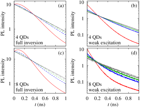
Figure 1: The PL signal under strong (a,c) and weak (b,d) excitation for an ensemble of 4 (a,b) and 8 (c,d) QDs, as a function of the ensemble inhomogeneity: $\sigma=0,5,10,30$ meV for solid red, dashed blue, dashed green, and dash-dotted grey lines, respectively. The black dotted lines show the exponential decay of PL from a single dot. All the curves are averaged over 100 QD ensembles.

In Fig. 1, we show the time dependence of the PL signal from systems of 4 and 8 QDs with a varying degree of spectral inhomogeneity. Under strong excitation, when the initial state is fully inverted (left panels), non-monotonic development of the PL signal is visible in the case of perfectly homogeneous ensembles (red solid lines), corresponding to the superradiant peak that would develop much more clearly in larger ensembles. A weak non-monotonicity is still visible for a weakly inhomogeneous ensemble ($\sigma=5$ meV, blue dashed line), while for the more inhomogeneous ensembles the PL decay is monotonic. Although the qualitative form of the time dependence of the PL signal becomes hardly distinguishable from exponential, the decay is noticeably faster than that corresponding to a single QD (shown with a black dotted line). Apart from a more pronounced maximum and a faster decay in the case of 8 QDs, there is no qualitative difference between the two ensemble sizes. Under weak excitation (linear response regime, right panels in Fig. 1), the PL decay is always monotonic. However, in a homogeneous or sufficiently weakly inhomogeneous system (red and blue lines) the PL decay is non-exponential. In a larger system this non-exponential behavior extends to larger values of inhomogeneity [green line, corresponding to $\sigma=10$ meV, in Fig. 1(d)] but eventually, for strongly inhomogeneous systems the decay also becomes exponential. Let us note at this point that in the experimentally studied ensemble scheibner07 , one had $\sigma\approx 18$ meV.

Comparison of the simulated PL dynamics in a fully inverted system [Fig. 1(a,c)] with that under weak excitation [Fig. 1(b,d)] leads to the first main conclusion of our analysis. A given system can emit in a different way depending on the initial excitation. In practice, the control of excitation conditions (initial state) may be limited. E.g., it may be hard to induce full inversion of all the QDs in the ensemble. Our results allow one to infer the dynamics of the system under full inversion based on the PL decay from the same system under weak excitation: If the system, when fully inverted, is able to show peaked, superradiant emission, then it manifests its superradiant properties already in the linear response (weak excitation) regime by a non-exponential decay of the PL signal. Conversely, a system in which, when excited weakly, the PL signal decays exponentially will show a monotonic decay, close to exponential, under strong inversion. In fact, especially for a system of 8 QDs, the weak excitation dynamics is non-exponential already for $\sigma=10$ meV, while the decay under full inversion in such an ensemble is monotonic and rather close to exponential apart from the initial phase of a few tens of picoseconds. Thus, the conditions for developing actual superradiance (in particular the spectral homogeneity of the system) are more strict than those allowing deviations from exponential decay in the linear response regime. It may also be interesting to note that the PL decay in inhomogeneous systems in the two excitation regimes, even though close to exponential in both cases, is still qualitatively different: the time dependence of the PL signal, when plotted in the logarithmic scale, is concave for strong inversion and convex in the linear response regime, at least for sufficiently short times (on the order of the PL life time).

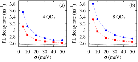
Figure 2: PL decay rates extracted from exponential fitting to the PL decay curves for 4 (a) and 8 (b) QDs. Blue circles and red squares correspond to weak and strong excitation regimes, respectively. Dashed lines are added to guide the eye. Black dotted lines show the decay rate for a single QD.

In view of the fact that the PL decay in an inhomogeneous system is close to exponential and can be indistinguishable from the latter based on actual experimental data it seems reasonable to extract the apparent decay rates from the PL evolution by fitting the PL curves with an exponential dependence. The result for the two ensemble sizes discussed above and for a series of values of $\sigma$ is shown in Fig. 2, where the blue circles and red squares correspond to weak and strong excitation, respectively. This result is the second main conclusion of this work: the PL signal under weak excitation decays faster than after fully inverting the system. This means that the spatial coherence generated by the global state preparation is higher than that achievable spontaneously by the inhomogeneous system in the evolution of the inverted state (contrary to the standard, highly symmetric case of non-interacting, identical atoms nussenzweig73 , where the system evolves via the subspace of maximally spatially coherent states).

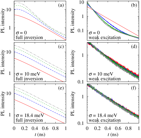
Figure 3: The time-resolved PL signal as a function of the QD ensemble size for three values of the ensemble inhomogeneity as shown and for the fully inverted (a,c,e) and weakly excited (b,d,f) initial state. Red solid: 2 QDs, blue dashed: 4 QDs, green dashed: 6 QDs, grey dash-dotted: 8 QDs.

For the sake of completeness, let us conclude our discussion with a brief analysis of how the PL signal evolves with growing ensemble size. The pertinent simulation results are presented in Fig. 3. In a strongly inverted homogeneous ensemble [Fig. 3(a)], non-monotonicity develops already for 3 or 4 QDs, in accordance with earlier findings for regular QD arrays sitek07a . This is again reflected by non-exponential decay under weak excitation [Fig. 3(b)]. For a realistic degree of inhomogeneity [Fig. 3(c-f)], the decay is only weakly non-exponential. For strong excitation, the PL intensities mostly differ by their magnitude (proportional to the number of the QDs) with only a small variation of the shape (flattening of the curve) at short times, which becomes stronger in larger ensembles. In a weakly excited inhomogeneous ensemble, the PL decay curves almost overlap and the difference of the decay rate becomes unnoticeable for $\sigma=18.4$ meV, which roughly corresponds to the ensemble studied in the experiment scheibner07 (nonetheless, more careful quantitative analysis shows that the rates do increase with the ensemble size kozub12 ).

IV Conclusions

We have modeled the evolution of the PL signal from homogeneous and inhomogeneous ensembles of a few (up to 8) coupled QDs. We focused on the comparison between the PL response under strong excitation (fully inverted initial state) and weak excitation (linear response).

We have shown that the signals from a given QD ensemble in the two regimes, although obviously different, are correlated: A system homogeneous enough to manifest non-monotonic, superradiant emission when strongly inverted shows a non-exponential decay of the PL signal under spatially coherent weak excitation. In a more inhomogeneous system the PL decay under weak excitation is close to exponential and so is the time-resolved PL signal under full occupation inversion. The QD samples in which collective emission was found experimentally scheibner07 belong to the latter class.

While the PL decay converges to the simple exponential form as the inhomogeneity grows, it retains a different character in the two excitation regimes, showing concave and convex behavior (in the logarithmic scale) for strong and weak excitation, respectively.

Quantitatively, when fitting the nearly exponential PL decay with a strictly exponential dependence, the decay under weak excitation appears faster than in the fully inverted case. Hence, simulations performed for weakly excited systems (which are much less demanding computationally) yield an upper bound on the apparent decay rates for a given system under any excitation intensity.

Acknowledgment: This work was supported in parts by the Polish National Science Centre (Grant No. DEC-2011/01/B/ST3/02415) and by the Foundation for Polish Science under the TEAM programme, co-financed by the European Regional Development Fund.

References

- (1) V. V. Temnov and U. Woggon, Phys. Rev. Lett. 95, 243602 (2005).
- (2) V. V. Temnov and U. Woggon, Opt. Express 17, 5774 (2009).
- (3) N. S. Averkiev, M. M. Glazov, and A. N. Poddubnyi, Zh. Eksp. Teor. Fiz. 108, 958 (2009), [J. Exp. Theor. Phys. 108, 836 (2009)].
- (4) V. I. Yukalov and E. P. Yukalova, Phys. Rev. B 81, 075308 (2010).
- (5) A. Auffèves, D. Gerace, S. Portolan, A. Drezet, and M. F. Santos, New J. Phys. 13, 093020 (2011).
- (6) M. Scheibner, T. Schmidt, L. Worschech, A. Forchel, G. Bacher, T. Passow, and D. Hommel, Nat. Phys. 3, 106 (2007).
- (7) Y. I. Mazur, V. G. Dorogan, J. E. Marega, G. G. Tarasov, D. F. Cesar, V. Lopez-Richard, G. E. Marques, and G. J. Salamo, Appl. Phys. Lett. 94, 123112 (2009).
- (8) E. W. Bogaart and J. E. M. Haverkort, J. Appl. Phys. 107, 064313 (2010).
- (9) S. M. Ulrich, C. Gies, S. Ates, J. Wiersig, S. Reitzenstein, C. Hofmann, A. Löffler, A. Forchel, F. Jahnke, and P. Michler, Phys. Rev. Lett. 98, 043906 (2007).
- (10) D. L. Boiko and P. P. Vasil’ev, Opt. Express 20, 9501 (2012).
- (11) J. Kasprzak, B. Patton, V. Savona, and W. Langbein, Nature Photonics 5, 57 (2010).
- (12) M. Kozub, Ł. Pawicki, and P. Machnikowski, Phys. Rev. B 86, 121305(R) (2012).
- (13) A. Sitek and P. Machnikowski, Phys. Rev. B 75, 035328 (2007).
- (14) A. Sitek and P. Machnikowski, Phys. Rev. B 80, 115319 (2009).
- (15) R. H. Dicke, Phys. Rev. 93, 99 (1954).
- (16) M. Gross and S. Haroche, Phys. Rep. 93, 301 (1982).
- (17) N. Skribanowitz, I. P. Herman, J. C. MacGilvray, and M. S. Feld, Phys. Rev. Lett. 30, 309 (1973).
- (18) M. J. Stephen, J. Chem. Phys. 40, 669 (1964).
- (19) R. H. Lehmberg, Phys. Rev. A 2, 883 (1970).
- (20) A. Varfolomeev, Zh. Eksp. Teor. Fiz. 59, 1702 (1970), [Sov. Phys.–JETP 32, 926 (1971)].
- (21) H. M. Nussenzweig, Introduction to Quantum Optics (Gordon and Breach, New York, 1973).