Treating $Z_{c}(3900)$ and $Z(4430)$ as the ground-state and first radially excited tetraquarks

Abstract

Exploration of the resonances $Z_{c}(3900)$ and $Z(4430)$ are performed by assuming that they are ground-state and first radial excitation of the same tetraquark with $J^{P}=1^{+}$. The mass and current coupling of the $Z_{c}(3900)$ and $Z(4430)$ states are calculated using QCD two-point sum rule method by taking into account vacuum condensates up to eight dimensions. We investigate the vertices $Z_{c}M_{h}M_{l}$ and $ZM_{h}M_{l}$, with $M_{h}$ and $M_{l}$ being the heavy and light mesons, and evaluate the strong couplings $g_{Z_{c}M_{h}M_{l}}$ and $g_{ZM_{h}M_{l}}$ using QCD sum rule on the light cone. The extracted couplings allow us to find the partial width of the decays $Z_{c}(3900)\to J/\psi\pi;\,\psi^{\prime}\pi;\,\eta_{c}\rho$ and $Z(4430)\to\psi^{\prime}\pi;\,J/\psi\pi;\,\eta_{c}^{\prime}\rho;\,\eta_{c}\rho$, which may help in comprehensive investigation of these resonances. We compare width of the decays of $Z_{c}(3900)$ and $Z(4430)$ resonances with available experimental data as well as existing theoretical predictions.

I Introduction

The discoveries of the charged $Z(4430)$ and $Z_{c}(3900)$ resonances had important consequences for the physics of multi-quark hadrons, because they could not be interpreted as neutral $\bar{c}c$ charmonia and became real candidates to tetraquark states. The $Z^{\pm}(4430)$ states were observed by the Belle Collaboration in $B$ meson decays $B\to K\psi^{\prime}\pi^{\pm}$ as resonances in the $\psi^{\prime}\pi^{\pm}$ invariant mass distribution Choi:2007wga . The resonances $Z^{+}(4430)$ and $Z^{-}(4430)$ were detected and studied later again by Belle in the processes $B\to K\psi^{\prime}\pi^{+}$ Mizuk:2009da and $B^{0}\to K^{+}\psi^{\prime}\pi^{-}$ Chilikin:2013tch , respectively. An evidence for $Z(4430)$ resonance decaying to $J/\psi\pi$ was found by the same collaboration in the process $\bar{B}^{0}\to J/\psi K^{-}\pi^{+}$ Chilikin:2014bkk . The available experimental information allowed the Belle Collaboration, apart from the masses and decay widths of these resonances, to fix also their spin-parity $J^{P}=1^{+}$ as a most favorable assumption among the $0^{-},\,1^{\pm}$ and $2^{\pm}$ options. The parameters of $Z^{-}(4430)$ were measured in the $B^{0}\to K^{+}\psi^{\prime}\pi^{-}$ decay by the LHCb Collaboration with the results

$$M=(4475\pm 7_{-25}^{+15})\,\mathrm{MeV},\,\Gamma=(172\pm 13_{-34}^{+37})\,\mathrm{MeV},$$ (1)

where its spin-parity was unambiguously determined to be $1^{+}$ Aaij:2014jqa ; Aaij:2015zxa .

Other members of the charged tetraquarks family, namely $Z_{c}^{\pm}(3900)$ were discovered by the BESIII Collaboration in the process $e^{+}e^{-}\to J/\psi\pi^{+}\pi^{-}$, as resonances in the $J/\psi\pi^{\pm}$ invariant mass distributions with the parameters

$$M=(3899.0\pm 3.6\pm 4.9)\,\mathrm{MeV},\,\Gamma=(46\pm 10\pm 20)\,\mathrm{MeV},$$ (2)

and spin-parity $J^{P}=1^{+}$ Ablikim:2013mio . These structures were observed also by the Belle and CLEO collaborations, as well (see, Refs. Liu:2013dau ; Xiao:2013iha ). Recently, BESIII announced the observation of the neutral $Z_{c}^{0}(3900)$ state in the process $e^{+}e^{-}\rightarrow\pi^{0}Z_{c}^{0}\rightarrow\pi^{0}\pi^{0}J/\psi$ Ablikim:2015tbp .

Theoretical investigations of the $Z(4430)$ and $Z_{c}(3900)$ resonances embrace a variety of models and computational schemes Chen:2016qju ; Esposito:2016noz . The aim is to reveal their internal quark-gluon structure and determine their parameters, such as the masses, current couplings (pole residues) and width of decay modes. Thus, $Z(4430)$ was interpreted as the diquark-antidiquark Liu:2008qx ; Ebert:2008kb ; Bracco:2008jj ; Maiani:2008zz ; Wang:2010rt ; Maiani:2014 ; Wang:2014vha , molecular state Lee:2007gs ; Liu:2008xz ; Braaten:2007xw ; Branz:2010sh ; Goerke:2016hxf , the threshold effect Rosner:2007mu and hadro-charmonium composite Dubynskiy:2008mq .

The situation formed around the theoretical interpretation of the $Z_{c}(3900)$ resonance does not differ considerably from activities intending to explain features of $Z(4430)$. Indeed, there are attempts to treat it as the tightly bound diquark-antidiquark state Dias:2013xfa ; Wang:2013vex ; Deng:2014gqa ; Agaev:2016dev , as the four-quark bound state composed of conventional mesons Wang:2013daa ; Wilbring:2013cha ; Dong:2013iqa ; Ke:2013gia ; Gutsche:2014zda ; Esposito:2014hsa ; Chen:2015igx ; Gong:2016hlt ; Ke:2016owt , or as the threshold cusp Swanson:2014tra ; Ikeda:2016zwx .

The interesting idea was suggested in Ref. Maiani:2014 to consider the $Z_{c}(3900)$ and $Z(4430)$ resonances as the ground and first radially excited states of the same diquark-antidiquark multiplet. This assumption was motivated by the main decay channels of these resonances,

$$Z_{c}^{\pm}(3900)\to J/\psi\pi^{\pm},\,\,Z^{\pm}(4430)\to\psi^{\prime}\pi^{\pm},$$ (3)

and also by observation that the mass difference between the $1S$ and $2S$ states $m_{\psi^{\prime}}-m_{J/\psi}$ is approximately equal to the mass splitting $m_{Z}-m_{Z_{c}}$. This idea was realized within the diquark-antidiquark model, and in the context of QCD sum rule approach in Ref. Wang:2014vha , where the masses and pole residues of $Z_{c}(3900)$ and $Z(4430)$ were obtained. The performed analysis in this work seems to confirm a suggestion made there. It should be noted that the decay modes of the resonances $Z_{c}(3900)$ and $Z(4430)$, which contain an important dynamical information on the structure of these states, were not considered within this scheme.

The mass and decay constant (current coupling) are important spectroscopic parameters of a conventional hadron or an exotic multi-quark state, which should be measured and calculated first of all. Therefore, not surprisingly all theoretical models and schemes proposed to explain the internal structure of tetraquarks and their properties start from analysis and computation of these parameters. Only after obtaining reasonable predictions for the mass and current coupling a model may claim to be a correct theory of a tetraquark candidate. But this is not enough to make robust conclusions on the nature of observed resonances. Indeed, experimental investigations include measurements of both the masses and widths of the observed resonances, and provide additional information on their spins and parities.

Almost all models of the resonances $Z_{c}(3900)$ and $Z(4430)$ correctly predict their masses. In some of theoretical papers the decay channels of these states were addressed, as well. Thus, the decays of the $Z^{\pm}(4430)$ states $Z^{\pm}(4430)\to J/\psi\pi^{\pm};\,\psi^{\prime}\pi^{\pm}$ were investigated within a phenomenological Lagrangian approach by interpreting it as a molecular state with the structure $D_{1}(2420)\bar{D}^{\star}+h.c.$ in Ref. Branz:2010sh . Unfortunately, in this paper $Z(4430)$ was treated as a state with spin-parity $J^{P}=0^{-},\,1^{-}$ excluded by recent measurements. The same decay modes $Z^{+}(4430)\to J/\psi\pi^{+};\,\psi^{\prime}\pi^{+}$ were revisited in a covariant quark model in Ref. Goerke:2016hxf .

The different decay modes of the $Z_{c}(3900)$ state in a diquark-antidiquark model were analyzed in Refs. Dias:2013xfa and Agaev:2016dev . The $Z_{c}^{+}(3900)\to J/\psi\pi^{+};\,\eta_{c}\rho;\,D^{+}\bar{D}^{\star 0}$ decays’ widths were computed in Ref. Dias:2013xfa using the three-point sum rule method, whereas in Ref. Agaev:2016dev widths of the $Z_{c}^{+}(3900)\to J/\psi\pi^{+};\,\eta_{c}\rho$ decays were found by means of the light cone sum rule (LCSR) approach and a technique of the soft-meson approximation. In both of these works $Z_{c}(3900)$ was considered as a state with the spin-parities $J^{PC}=1^{+-}$.

The decays of the $Z_{c}^{\pm}(3900)$ resonances were a subject of studies in the framework of alternative methods Dong:2013iqa ; Gutsche:2014zda ; Goerke:2016hxf , as well. Thus, the decay channels $Z_{c}(3900)\to J/\psi\pi;\,\psi^{\prime}\pi;h_{c}(1P)\pi$ were calculated in a phenomenological Lagrangian approach by modeling $Z_{c}(3900)$ as a hadronic molecule $\bar{D}D^{\star}$ with $J^{P}=1^{+}$ Dong:2013iqa . The radiative and leptonic decays $Z_{c}^{+}(3900)\to J/\psi\pi^{+}\gamma$ and $J/\psi\pi^{+}l^{+}l^{-},\,l=(e,\,\mu)$ in the context of the same method were considered in Ref. Gutsche:2014zda . The widths of the decay modes $Z_{c}^{+}(3900)\to J/\psi\pi^{+};\,\eta_{c}\rho^{+};\bar{D}^{0}D^{\star+};\,\bar{D}^{\star 0}D^{+}$ were extracted in Ref. Goerke:2016hxf in a covariant quark model. Let us note also the work Ke:2016owt , where the $Z_{c}(3900)\to h_{c}\pi$ decay was analyzed in the light front model.

In the present study we are going to calculate the masses and current couplings of the $Z_{c}(3900)$ and $Z(4430)$ resonances, and investigate some of their decay modes. We assume that these resonances are the ground and first radially excited states of the tetraquark with $J^{P}=1^{+}$, i.e. we consider them as the axial-vector members of the $1S$ and $2S$ tetraquark multiplets. We will evaluate the mass and current coupling of the excited $Z(4430)$ state and width of the process $Z(4430)\to\psi^{\prime}\pi$, which is the main decay channel of $Z(4430)$ to examine correctness of the suggestion made on its nature. Other decay modes of the $Z(4430)$ resonance, namely $Z(4430)\to J/\psi\pi;\,\eta_{c}^{\prime}\rho;\,\eta_{c}\rho$ will be analyzed, as well. We will also calculate the $Z_{c}(3900)$ resonance’s parameters and its decay widths with higher accuracy than it was done in our previous work Agaev:2016dev . We will include into analysis also the decay mode $Z_{c}(3900)\to\psi^{\prime}\pi$, which was not considered in the previous paper.

This work is organized in the following form. In Sec. II we derive the spectral density $\rho^{\mathrm{QCD}}(s)$ from the two-point QCD sum rule by including condensates up to eight dimensions. This allows us to evaluate the mass and current coupling of the $Z_{c}(3900)$ and $Z(4430)$ with desired accuracy. The Sec. III is devoted to decays of the $Z_{c}(3900)$ and $Z(4430)$ states. Here we calculate relevant spectral densities with dimension-eight accuracy and find the width of the decays under consideration. Appendix contains the quark propagators used in this work, as well as explicit expressions of the spectral densities used in computation of the strong couplings.

II Masses and current couplings of the $Z_{c}(3900)$ and $Z(4430)$ resonances

In this section we calculate the masses and current couplings of the resonances $Z_{c}(3900)$ and $Z(4430)$. We consider the positively charged states with the quark content $\bar{c}cu\bar{d}$, but due to the exact chiral limit adopted in the present work, the parameters of the resonances with opposite charges do not differ from each other.

The masses and current couplings of the resonances under consideration can be extracted from analysis of the correlation function

$$\Pi_{\mu\nu}(p)=i\int d^{4}xe^{ip\cdot x}\langle 0|\mathcal{T}\{J_{\mu}^{Z}(x)J_{\nu}^{Z\dagger}(0)\}|0\rangle,$$ (4)

where the interpolating current with the quantum numbers $J^{PC}=1^{+-}$ is given by the following expression

$$J_{\nu}^{Z}(x) = \frac{i\epsilon\tilde{\epsilon}}{\sqrt{2}}\left\{\left[u_{a}^{T}(x)C\gamma_{5}c_{b}(x)\right]\left[\overline{d}_{d}(x)\gamma_{\nu}C\overline{c}_{e}^{T}(x)\right]\right.$$ (5)

$$\left.-\left[u_{a}^{T}(x)C\gamma_{\nu}c_{b}(x)\right]\left[\overline{d}_{d}(x)\gamma_{5}C\overline{c}_{e}^{T}(x)\right]\right\}.$$

Here we have introduced the notations $\epsilon=\epsilon_{abc}$ and $\tilde{\epsilon}=\epsilon_{dec}$. In Eq. (5) $a,b,c,d,e$ are color indices and $C$ is the charge conjugation operator.

We first derive the sum rules for the mass $m_{Z_{c}}$ and current coupling $f_{Z_{c}}$ of the ground state tetraquark $Z_{c}$. To this end, we use the ”ground-state + continuum” approximation by including the $Z(4430)$ state into the list of ”higher resonances” and extract corresponding sum rules. The mass and current coupling of $Z_{c}$ evaluated from these expressions are considered as input parameters in the sum rules for the excited $Z(4430)$ tetraquark.

At the next stage of calculations we adopt the ”ground-state+radially excited state+continuum” scheme, and perform the required standard manipulations: we derive the phenomenological side of the sum rules by inserting into the correlation function full sets of relevant states, by isolating contributions of the $Z_{c}$ and $Z$ resonances and carrying out the integration over $x$. As a result, for $\Pi_{\mu\nu}^{\mathrm{Phys}}(p)$ we get

$$\Pi_{\mu\nu}^{\mathrm{Phys}}(p)=\frac{\langle 0|J_{\mu}^{Z}|Z_{c}(p)\rangle\langle Z_{c}(p)|J_{\nu}^{Z\dagger}|0\rangle}{m_{Z_{c}}^{2}-p^{2}}$$

$$+\frac{\langle 0|J_{\mu}^{Z}|Z(p)\rangle\langle Z(p)|J_{\nu}^{Z\dagger}|0\rangle}{m_{Z}^{2}-p^{2}}+\ldots$$ (6)

where $m_{Z_{c}}$ and $m_{Z}$ are the masses of $Z_{c}(3900)$ and $Z(4430)$ states, respectively. The dots in Eq. (6) denote contributions arising from higher resonances and continuum states.

In order to finish computations of the sum rules’ phenomenological side we introduce the current couplings $f_{Z_{c}}$ and $f_{Z}$ through the matrix elements

$$\langle 0|J_{\mu}^{Z}|Z_{c}\rangle=f_{Z_{c}}m_{Z_{c}}\varepsilon_{\mu},\,\,\langle 0|J_{\mu}^{Z}|Z\rangle=f_{Z}m_{Z}\tilde{\varepsilon}_{\mu},$$ (7)

with $\varepsilon_{\mu}$ and $\tilde{\varepsilon}_{\mu}$ being the polarization vectors of the $Z_{c}$ and $Z$ states, respectively. Then the function $\Pi_{\mu\nu}^{\mathrm{Phys}}(p)$ can be written as

$$\Pi_{\mu\nu}^{\mathrm{Phys}}(p)=\frac{m_{Z_{c}}^{2}f_{Z_{c}}^{2}}{m_{Z_{c}}^{2}-p^{2}}\left(-g_{\mu\nu}+\frac{p_{\mu}p_{\nu}}{m_{Z_{c}}^{2}}\right)$$

$$+\frac{m_{Z}^{2}f_{Z}^{2}}{m_{Z}^{2}-p^{2}}\left(-g_{\mu\nu}+\frac{p_{\mu}p_{\nu}}{m_{Z}^{2}}\right)+\ldots$$ (8)

The Borel transformation applied to Eq. (8) yields

$$\mathcal{B}_{p^{2}}\Pi_{\mu\nu}^{\mathrm{Phys}}(p)=m_{Z_{c}}^{2}f_{Z_{c}}^{2}e^{-m_{Z_{c}}^{2}/M^{2}}\left(-g_{\mu\nu}+\frac{p_{\mu}p_{\nu}}{m_{Z_{c}}^{2}}\right)$$

$$+m_{Z}^{2}f_{Z}^{2}e^{-m_{Z}^{2}/M^{2}}\left(-g_{\mu\nu}+\frac{p_{\mu}p_{\nu}}{m_{Z}^{2}}\right)+\ldots,$$ (9)

where $M^{2}$ is the Borel parameter.

The QCD side of the sum rules $\Pi_{\mu\nu}^{\mathrm{QCD}}(q)$ can be determined using the interpolating current $J_{\nu}^{Z}$ and quark propagators, explicit expressions of which can be found in Appendix. Thus, after contracting the heavy and light quark fields in Eq. (4) we get

$$\Pi_{\mu\nu}^{\mathrm{QCD}}(p)=-\frac{i}{2}\int d^{4}xe^{ipx}\epsilon\tilde{\epsilon}\epsilon^{\prime}\tilde{\epsilon}^{\prime}\left\{\mathrm{Tr}\left[\gamma_{5}\widetilde{S}_{u}^{aa^{\prime}}(x)\right.\right.$$

$$\times\left.\gamma_{5}S_{c}^{bb^{\prime}}(x)\right]\mathrm{Tr}\left[\gamma_{\mu}\widetilde{S}_{c}^{e^{\prime}e}(-x)\gamma_{\nu}S_{d}^{d^{\prime}d}(-x)\right]$$

$$-\mathrm{Tr}\left[\gamma_{\mu}\widetilde{S}_{c}^{e^{\prime}e}(-x)\gamma_{5}S_{d}^{d^{\prime}d}(-x)\right]\mathrm{Tr}\left[\gamma_{\nu}\widetilde{S}_{u}^{aa^{\prime}}(x)\gamma_{5}S_{c}^{bb^{\prime}}(x)\right]$$

$$-\mathrm{Tr}\left[\gamma_{5}\widetilde{S}_{u}^{a^{\prime}a}(x)\gamma_{\mu}S_{c}^{b^{\prime}b}(x)\right]\mathrm{Tr}\left[\gamma_{5}\widetilde{S}_{c}^{e^{\prime}e}(-x)\gamma_{\nu}S_{d}^{d^{\prime}d}(-x)\right]$$

$$\left.+\mathrm{Tr}\left[\gamma_{\nu}\widetilde{S}_{u}^{aa^{\prime}}(x)\gamma_{\mu}S_{c}^{bb^{\prime}}(x)\right]\mathrm{Tr}\left[\gamma_{5}\widetilde{S}_{c}^{e^{\prime}e}(-x)\gamma_{5}S_{d}^{d^{\prime}d}(-x)\right]\right\},$$

where

$$\widetilde{S}_{c(q)}^{ij}(x)=CS_{c(q)}^{ij\mathrm{T}}(x)C.$$

The function $\Pi_{\mu\nu}^{\mathrm{QCD}}(p)$ has the following decomposition over the Lorentz structures

$$\Pi_{\mu\nu}^{\mathrm{QCD}}(p)=\Pi^{\mathrm{QCD}}(p^{2})(-g_{\mu\nu})+\widetilde{\Pi}^{\mathrm{QCD}}(p^{2})p_{\mu}p_{\nu}.$$ (11)

The required QCD sum rules for the parameters of $Z(4430)$ can be obtained after equating the same structures in both $\Pi_{\mu\nu}^{\mathrm{Phys}}(p)$ and $\Pi_{\mu\nu}^{\mathrm{QCD}}(p)$. For our purposes the convenient structures are terms $\sim(-g_{\mu\nu})$, which we employ in further calculations.

The invariant amplitude corresponding to the structure $-g_{\mu\nu}$ in $\Pi_{\mu\nu}^{\mathrm{Phys}}(p)$ has the simple form. The similar function $\Pi^{\mathrm{QCD}}(p^{2})$ can be represented as the dispersion integral

$$\Pi^{\mathrm{QCD}}(p^{2})=\int_{4m_{c}^{2}}^{\infty}\frac{\rho^{\mathrm{QCD}}(s)}{s-p^{2}}ds,$$ (12)

where $\rho^{\mathrm{QCD}}(s)$ is the two-point spectral density. Methods to derive $\rho^{\mathrm{QCD}}(s)$ as the imaginary part of the correlation function are well known, therefore we skip here details of standard calculations, and also refrain from providing its explicit expression.

We apply the Borel transformation on the variable $p^{2}$ to both the phenomenological and QCD sides of the equality and subtract the contributions of the higher resonances and continuum states by invoking the assumption on the quark-hadron duality. After simple manipulations we derive the sum rules for the mass and current coupling of the excited $Z(4430)$ state:

$$m_{Z}^{2}=\frac{\int_{4m_{c}^{2}}^{s_{0}^{\ast}}\rho^{\mathrm{QCD}}(s)se^{-s/M^{2}}ds-f_{Z_{c}}^{2}m_{Z_{c}}^{4}e^{-m_{Z_{c}}^{2}/M^{2}}}{\int_{4m_{c}^{2}}^{s_{0}^{\ast}}\rho^{\mathrm{QCD}}(s)e^{-s/M^{2}}ds-f_{Z_{c}}^{2}m_{Z_{c}}^{2}e^{-m_{Z_{c}}^{2}/M^{2}}},$$ (13)

and

$$f_{Z}^{2} = \frac{1}{m_{Z}^{2}}\left[\int_{4m_{c}^{2}}^{s_{0}^{\ast}}\rho^{\mathrm{QCD}}(s)e^{(m_{Z}^{2}-s)/M^{2}}ds\right.$$ (14)

$$\left.-f_{Z_{c}}^{2}m_{Z_{c}}^{2}e^{(m_{Z}^{2}-m_{Z_{c}}^{2})/M^{2}}\right],$$

where $s_{0}^{\ast}$ is the continuum threshold parameter, which separates the contributions of the ”$Z_{c}$ +$Z$” states from the contributions due to ”higher resonances and continuum”. As we have emphasized above the mass and current coupling of $Z_{c}$ enter into Eqs. (13) and (14) as the input parameters. The mass of the $Z_{c}$ state can be found from the sum rule

$$m_{Z_{c}}^{2}=\frac{\int_{4m_{c}^{2}}^{s_{0}}ds\rho^{\mathrm{QCD}}(s)se^{-s/M^{2}}}{\int_{4m_{c}^{2}}^{s_{0}}ds\rho^{\mathrm{QCD}}(s)e^{-s/M^{2}}},$$ (15)

whereas to extract the numerical value of the decay constant $f_{Z_{c}}$ we employ the formula

$$f_{Z_{c}}^{2}=\frac{1}{m_{Z_{c}}^{2}}\int_{4m_{c}^{2}}^{s_{0}}ds\rho^{\mathrm{QCD}}(s)e^{(m_{Z_{c}}^{2}-s)/M^{2}}.$$ (16)

In Eqs. (15) and (16) $s_{0}$ is the continuum threshold, which divides the contributions of the ground-state $Z_{c}(3900)$ and higher resonances and continuum. It is evident, that sum rules depend on the same spectral density $\rho^{\mathrm{QCD}}(s)$, and the continuum threshold has to obey $s_{0}<s_{0}^{\star}$.

The expressions obtained in the present work contain the vacuum expectations values of the different operators, which are input parameters in the numerical calculations. These vacuum condensates are well known: for the quark and mixed condensates we use $\langle\bar{q}q\rangle=-(0.24\pm 0.01)^{3}~{}\mathrm{GeV}^{3}$ and $\langle\overline{q}g_{s}\sigma Gq\rangle=m_{0}^{2}\langle\bar{q}q\rangle$, where $m_{0}^{2}=(0.8\pm 0.1)~{}\mathrm{GeV}^{2}$, whereas for the gluon condensates we utilize $\langle\alpha_{s}G^{2}/\pi\rangle=(0.012\pm 0.004)~{}\mathrm{GeV}^{4}$ and $\langle g_{s}^{3}G^{3}\rangle=(0.57\pm 0.29)~{}\mathrm{GeV}^{6}$.

The sum rules depend also on the auxiliary parameters $M^{2}$ and $s_{0}(s_{0}^{\star})$, which have to meet requirements of the sum rule computations. In other words, the bounds of working region for the Borel parameter are fixed by the convergence of the operator product expansion and dominance of the pole contribution to the whole expression. Additionally, regions within of which the parameters $M^{2}$ and $s_{0}$ can be varied should provide stability domains of extracted quantities on the parameters $M^{2}$ and $s_{0}$. Performed analysis allows us to fix regions of the parameters $M^{2}$ and $s_{0}$, where the aforementioned conditions are satisfied. Numerical results of our calculations are collected in Table 1, where we write down not only the mass and current couplings of the resonances $Z(4430)$ and $Z_{c}(3900)$, but also regions of the parameters used in their evaluation. It is seen that $m_{Z_{c}}$ is in excellent agreement with the experimental data. It also almost coincide with our previous result for $m_{Z_{c}}$ obtained in Ref. Agaev:2016dev . Prediction for $m_{Z}$ is smaller than the corresponding LHCb result, but within errors of calculations it is compatible with measurements.

In Figs. 1 and 2 we demonstrate the dependence of $m_{Z}$ and $f_{Z}$ on $M^{2}$ at fixed $s_{0}$, and as functions of $s_{0}$ for chosen values of $M^{2}$. As is seen, the mass of the $Z(4430)$ resonance is rather stable against variations both of $M^{2}$ and $s_{0}$, whereas a sensitivity of $f_{Z}$ to changes of the auxiliary parameters is higher. The explanation here is quite simple: indeed, the sum rules for the mass of the resonances are given as ratios of integrals over the spectral densities $\rho(s)$ and $s\rho(s)$, which considerably reduce effects due to variations of $M^{2}$ and $s_{0}$. Contrary, the current couplings depend on mentioned integrals themselves, and therefore undergone relatively sizable changes. Thus, theoretical errors for $f_{Z_{c}}$ and $f_{Z}$ stemming from uncertainties of $M^{2}$ and $s_{0}$, and other input parameters equal to $\sim 19\%$ and $\sim 28\%$ of the central values, respectively. Nevertheless, they remain within allowed ranges for theoretical errors inherent to sum rule computations which may amount up to $30\%$ of predictions.

Resonance	$Z_{c}(3900)$	$Z(4430)$
$M^{2}~{}(\mathrm{GeV}^{2}$)	$3-6$	$3-6$
$s_{0}(s_{0}^{\star})~{}(\mathrm{GeV}^{2}$)	$4.2^{2}-4.4^{2}$	$4.8^{2}-5.2^{2}$
$m_{Z}~{}(\mathrm{MeV})$	$3901^{+125}_{-148}$	$4452^{+182}_{-228}$
$f_{Z}\cdot 10^{2}~{}(\mathrm{GeV}^{4})$	$0.42^{+0.07}_{-0.09}$	$1.48^{+0.31}_{-0.42}$

Table 1: The masses and current couplings of the $Z_{c}(3900)$ and $Z(4430)$ resonances evaluated in this work.

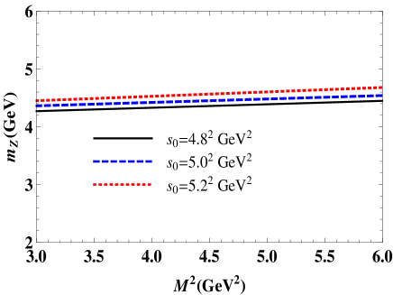
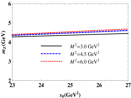
Figure 1: The mass of the state $Z(4430)$ as a function of the Borel parameter $M^{2}$ at fixed $s_{0}$ (left panel), and as a function of the continuum threshold $s_{0}$ at fixed $M^{2}$ (right panel).

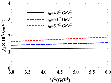
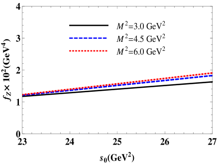
Figure 2: The dependence of the current coupling $f_{Z}$ of the $Z(4430)$ resonance on the Borel parameter at chosen values of $s_{0}$ (left panel), and on $s_{0}$ at fixed $M^{2}$ (right panel).

III Decays of the resonances $Z_{c}(3900)$ and $Z(4430)$

The masses of $Z_{c}(3900)$ and $Z(4430)$ extracted in the previous section can be used to fix kinematically allowed decay modes of these resonances. Moreover, their masses and current couplings enter as input parameters to expressions of the strong couplings describing vertices $Z_{c}M_{h}M_{l}$ and $ZM_{h}M_{l}$, and appear also in formulas for decay widths.

The resonances $Z_{c}(3900)$ and $Z(4430)$ may decay through different channels. In this work we restrict ourselves by analysis of their decays to $J/\psi\pi$, $\psi^{\prime}\pi$, and $\eta_{c}\rho$, $\eta_{c}^{\prime}\rho$ mesons: from Table 2, where we provide masses and decay constants of the relevant mesons, it is easy to realize that these decays are among kinematically allowed channels.

In this work we treat the $Z(4430)$ tetraquark as the first radial excitation of $Z_{c}(3900)$. Additionally, $\psi^{\prime}$ and $\eta_{c}^{\prime}$ are the first radial excitations of the mesons $J/\psi$ and $\eta_{c}$, respectively. Therefore, we have to consider decays $Z_{c}(3900),\,Z(4430)\to J/\psi\pi;\,\psi^{\prime}\pi$ and $Z_{c}(3900),\,Z(4430)\to\eta_{c}\rho;\,\eta_{c}^{\prime}\rho$ in the context of QCD sum rule approach in a correlated form. Reasons behind of such analysis are clear. In fact, in QCD sum rule method particles are modeled by relevant interpolating currents which may couple not only to their ground-states, but also to excited particles.

Parameters	Values (in $\mathrm{MeV}$)
$m_{J/\psi}$	$3096.900\pm 0.006$
$f_{J/\psi}$	$411\pm 7$
$m_{\psi^{\prime}}$	$3686.097\pm 0.025$
$f_{\psi^{\prime}}$	$279\pm 8$
$m_{\eta_{c}}$	$2983.4\pm 0.5$
$f_{\eta_{c}}$	$404$
$m_{\eta_{c}^{\prime}}$	$3686.2\pm 1.2$
$f_{\eta_{c}^{\prime}}$	$331$
$m_{\pi}$	$139.57018\pm 0.00035$
$f_{\pi}$	$131.5$
$m_{\rho}$	$775.26\pm 0.25$
$f_{\rho}$	$216\pm 3$
$m_{c}$	$1270\pm 30$

Table 2: Input parameters.

III.1 $Z_{c}(3900),\,Z(4430)\to J/\psi\pi;\,\psi^{\prime}\pi$ decays

In order to find width of the decays $Z_{c}(3900)\rightarrow J/\psi\pi,\,\psi^{\prime}\pi$ and $Z(4430)\rightarrow J/\psi\pi;\,\psi^{\prime}\pi$ we start from the correlation function

$$\Pi_{\mu\nu}(p,q)=i\int d^{4}xe^{ipx}\langle\pi(q)|\mathcal{T}\{J_{\mu}^{\psi}(x)J_{\nu}^{Z\dagger}(0)\}|0\rangle,$$ (17)

where

$$J_{\mu}^{\psi}(x)=\overline{c}_{i}(x)\gamma_{\mu}c_{i}(x),$$ (18)

and $\psi$ denotes one of  the $J/\psi$ and $\psi^{\prime}$ mesons. The interpolating current $J_{\nu}^{Z}(x)$ for the tetraquarks is defined by Eq. (5). As we have just emphasized above the interpolating currents $J_{\nu}^{Z}(x)$ and $J_{\mu}^{\psi}(x)$ couple to $Z_{c}(3900),\,Z(4430)$ and $J/\psi,\,\psi^{\prime}$, respectively. Therefore, the correlation function $\Pi_{\mu\nu}^{\mathrm{Phys}}(p,q)$ necessary for our purposes in terms of the mesons’ physical parameters contains four terms

$$\Pi_{\mu\nu}^{\mathrm{Phys}}(p,q)=\sum_{\psi=J/\psi,\psi^{\prime}}\left[\frac{\langle 0|J_{\mu}^{\psi}|\psi\left(p\right)\rangle}{p^{2}-m_{\psi}^{2}}\langle\psi\left(p\right)\pi(q)|Z_{c}(p^{\prime})\rangle\right.$$

$$\times\frac{\langle Z_{c}(p^{\prime})|J_{\nu}^{Z\dagger}|0\rangle}{p^{\prime 2}-m_{Z_{c}}^{2}}+\frac{\langle 0|J_{\mu}^{\psi}|\psi\left(p\right)\rangle}{p^{2}-m_{\psi}^{2}}\langle\psi\left(p\right)\pi(q)|Z(p^{\prime})\rangle$$

$$\left.\times\frac{\langle Z(p^{\prime})|J_{\nu}^{Z\dagger}|0\rangle}{p^{\prime 2}-m_{Z}^{2}}\right]+\dots,$$ (19)

where the dots stand for contribution of the higher resonances and continuum states and $p^{\prime}=p+q$.

To calculate the correlation function we introduce the matrix elements

$$\langle 0|J_{\mu}^{\psi}|\psi\left(p\right)\rangle=f_{\psi}m_{\psi}\varepsilon_{\mu},\,\,\langle Z_{c}(p^{\prime})|J_{\nu}^{Z\dagger}|0\rangle=f_{Z_{c}}m_{Z_{c}}\varepsilon_{\nu}^{\prime\ast},$$

$$\langle Z(p^{\prime})|J_{\nu}^{Z\dagger}|0\rangle=f_{Z}m_{Z}\widetilde{\varepsilon}_{\nu}^{\prime\ast},$$ (20)

where $f_{\psi},\,m_{\psi},\,\varepsilon_{\mu}$ are the decay constant, mass and polarization vector of $J/\psi$ or $\psi^{\prime}$ meson, whereas $\widetilde{\varepsilon}_{\nu}^{\prime}$ and $\varepsilon_{\nu}^{\prime}$ are the polarization vectors of $Z$ and $Z_{c}$ states, respectively

We need also the vertices

$$\langle\psi\left(p\right)\pi(q)|Z_{c}(p^{\prime})\rangle = g_{Z_{c}\psi\pi}\left[(p\cdot p^{\prime})(\varepsilon^{\ast}\cdot\varepsilon^{\prime})\right.$$

$$\left.-(p\cdot\varepsilon^{\prime})(p^{\prime}\cdot\varepsilon^{\ast})\right],$$

$$\langle\psi\left(p\right)\pi(q)|Z(p^{\prime})\rangle = g_{Z\psi\pi}\left[(p\cdot p^{\prime})(\varepsilon^{\ast}\cdot\widetilde{\varepsilon}^{\prime})\right.$$ (21)

$$\left.-(p\cdot\widetilde{\varepsilon}^{\prime})(p^{\prime}\cdot\varepsilon^{\ast})\right],$$

with $g_{Z_{c}\psi\pi}$ and $g_{Z\psi\pi}$ being the strong couplings, which should be determined from sum rules. By using Eqs. (20) and (21) and after some manipulations we get

$$\Pi_{\mu\nu}^{\mathrm{Phys}}(p,q)=\sum_{\psi=J/\psi,\psi^{\prime}}\left[\frac{f_{\psi}f_{Z_{c}}m_{Z_{c}}m_{\psi}g_{Z_{c}\psi\pi}}{\left(p^{\prime 2}-m_{Z_{c}}^{2}\right)\left(p^{2}-m_{\psi}^{2}\right)}\right.$$

$$\times\left(\frac{m_{Z_{c}}^{2}+m_{\psi}^{2}}{2}g_{\mu\nu}-p_{\mu}^{\prime}p_{\nu}\right)+\frac{f_{\psi}f_{Z}m_{Z}m_{\psi}g_{Z\psi\pi}}{\left(p^{\prime 2}-m_{Z}^{2}\right)\left(p^{2}-m_{\psi}^{2}\right)}$$

$$\left.\times\left(\frac{m_{Z}^{2}+m_{\psi}^{2}}{2}g_{\mu\nu}-p_{\mu}^{\prime}p_{\nu}\right)\right]+\ldots.$$ (22)

For further calculations we choose the structure $\sim g_{\mu\nu}$. The sum of terms $\sim g_{\mu\nu}$ from Eq. (22) constitute the invariant function which will be used in the following analysis.

The second component of the sum rule is the expression of the same correlation function given by Eq. (17), but computed using quark propagators. For $\Pi_{\mu\nu}^{\mathrm{QCD}}(p,q)$ we find

$$\Pi_{\mu\nu}^{\mathrm{QCD}}(p,q)=\int d^{4}xe^{ipx}\frac{\epsilon\widetilde{\epsilon}}{\sqrt{2}}\left[\gamma_{5}\widetilde{S}_{c}^{ib}(x){}\gamma_{\mu}\right.$$

$$\left.\times\widetilde{S}_{c}^{ei}(-x){}\gamma_{\nu}+\gamma_{\nu}\widetilde{S}_{c}^{ib}(x){}\gamma_{\mu}\widetilde{S}_{c}^{ei}(-x){}\gamma_{5}\right]_{\alpha\beta}$$

$$\times\langle\pi(q)|\overline{u}_{\alpha}^{a}(0)d_{\beta}^{d}(0)|0\rangle,$$ (23)

where $\alpha$ and $\beta$ are the spinor indices. We continue by employing the expansion

$$\overline{u}_{\alpha}^{a}d_{\beta}^{d}\rightarrow\frac{1}{4}\Gamma_{\beta\alpha}^{j}\left(\overline{u}^{a}\Gamma^{j}d^{d}\right),$$ (24)

where $\Gamma^{j}$ is the full set of Dirac matrices

$$\Gamma^{j}=\mathbf{1,\ }\gamma_{5},\ \gamma_{\lambda},\ i\gamma_{5}\gamma_{\lambda},\ \sigma_{\lambda\rho}/\sqrt{2},$$

As is seen, $\Pi_{\mu\nu}^{\mathrm{QCD}}(p,q)$ instead of the distribution amplitudes of the pion depends on its local matrix elements. This is distinctive feature of QCD sum rules on the light-cone when one of the particles is a tetraquark. As a result, to conserve the four-momentum in the tetraquark-meson-meson vertex one has to set $q=0$ Agaev:2016dev ; Agaev:2017foq . This restriction should be implemented in the physical side of the sum rule, as well. In the standard LCSR, $q=0$ is known as the soft-meson approximation Belyaev:1994zk . At vertices composed of conventional mesons $q\neq 0$, and only in the soft-meson approximation one equals $q$ to zero, whereas the tetraquark-meson-meson vertex can be considered in the framework of the LCSR method only if $q=0$. For our purposes a decisive fact is the observation made in Ref. Belyaev:1994zk : both the soft-meson approximation and full LCSR treatment of the ordinary mesons’ vertices for the strong couplings lead to results which numerically are very close to each other.

After substituting Eq. (24) into the expression of the correlation function and performing the summation over color indices in accordance with prescriptions presented in a detailed form in Ref. Agaev:2016dev , we determine a local matrix element of the pion that contribute to $\Pi_{\mu\nu}^{\mathrm{QCD}}(p,q)$, and find the corresponding spectral density $\rho^{\mathrm{QCD}}(s)$ as its imaginary part. It turns out that only the local matrix element of the pion

$$\langle 0|\overline{d}(0)i\gamma_{5}u(0)|\pi(q)\rangle=f_{\pi}\mu_{\pi}$$ (25)

contribute to $\rho^{\mathrm{QCD}}(s)$, where $\mu_{\pi}=m_{\pi}^{2}/(m_{u}+m_{d})$.

To calculate $\rho^{\mathrm{QCD}}(s)$ we choose in $\Pi_{\mu\nu}^{\mathrm{QCD}}(p,q)$ again the structure $\sim g_{\mu\nu}$, and get

$$\rho^{\mathrm{QCD}}(s)=\frac{f_{\pi}\mu_{\pi}}{12\sqrt{2}}\left[\rho^{\mathrm{pert.}}(s)+\rho^{\mathrm{n.-pert.}}(s)\right],$$ (26)

where $\rho^{\mathrm{pert.}}(s)$ and $\rho^{\mathrm{n.-pert.}}(s)$ are the perturbative and nonperturbative components of the spectral density. The perturbative part of $\rho^{\mathrm{QCD}}(s)$ has a rather simple form and was calculated in Ref. Agaev:2016dev :

$$\rho^{\mathrm{pert.}}(s)=\frac{(s+2m_{c}^{2})\sqrt{s(s-4m_{c}^{2})}}{\pi^{2}s}.$$ (27)

The $\rho^{\mathrm{n.-pert.}}(s)$ contains nonperturbative contributions $\sim\langle\alpha_{s}G^{2}/\pi\rangle$, $\sim\langle g_{s}^{3}G^{3}\rangle$ and $\sim\langle\alpha_{s}G^{2}/\pi\rangle^{2}$ which are terms of four, six and eight dimensions, respectively. Stated differently, $\rho^{\mathrm{n.-pert.}}(s)$ encompasses nonperturbative contributions up to eight dimensions: its explicit expression is moved to Appendix.

Having found $\rho^{\mathrm{QCD}}(s)$ which constitutes the QCD side of the desiring sum rule, and clarified the necessity of the limit $q\rightarrow 0$, we turn back to finish calculation of its phenomenological side. In the limit $q\rightarrow 0$ we get $p^{\prime}=p$ and invariant function corresponding to the structure $g_{\mu\nu}$ in Eq. (19) depends only on the variable $p^{2}$ and has the form

$$\Pi^{\mathrm{Phys}}(p^{2})=\frac{f_{J/\psi}f_{Z_{c}}m_{Z_{c}}m_{J/\psi}m_{1}^{2}}{\left(p^{2}-m_{1}^{2}\right)^{2}}g_{Z_{c}J/\psi\pi}$$

$$+\frac{f_{\psi^{\prime}}f_{Z_{c}}m_{Z_{c}}m_{\psi^{\prime}}m_{2}^{2}}{\left(p^{2}-m_{2}^{2}\right)^{2}}g_{Z_{c}\psi^{\prime}\pi}+\frac{f_{J/\psi}f_{Z}m_{Z}m_{J/\psi}m_{3}^{2}}{\left(p^{2}-m_{3}^{2}\right)^{2}}g_{ZJ/\psi\pi}$$

$$+\frac{f_{\psi^{\prime}}f_{Z}m_{Z}m_{\psi^{\prime}}m_{4}^{2}}{\left(p^{2}-m_{4}^{2}\right)^{2}}g_{Z\psi^{\prime}\pi}+\ldots,$$ (28)

where $m_{1}^{2}=(m_{Z_{c}}^{2}+m_{J/\psi}^{2})/2$, $m_{2}^{2}=(m_{Z_{c}}^{2}+m_{\psi^{\prime}}^{2})/2$,$\ m_{3}^{2}=(m_{Z}^{2}+m_{J/\psi}^{2})/2$, and $m_{4}^{2}=(m_{Z}^{2}+m_{\psi^{\prime}}^{2})/2$.

In the limit $q\rightarrow 0$ the phenomenological side of the sum rules apart from the strong coupling of the ground-state particles $g_{Z_{c}J/\psi\pi}$ contains also other terms which are not suppressed relative to the main term even after the Borel transformation Belyaev:1994zk . In order to eliminate their effects the operator

$$\mathcal{P}(M^{2},m^{2})=\left(1-M^{2}\frac{d}{dM^{2}}\right)M^{2}e^{m^{2}/M^{2}},$$ (29)

should be applied to both sides of sum rules Ioffe:1983ju . In our previous works devoted to investigation of tetraquarks for calculation of their strong couplings and decay widths we applied namely this technique (see, for example Refs. Agaev:2016dev ; Agaev:2017foq ). But these terms arise from vertices composed of excited states of the initial (final) particles, i.e. in our case from $ZJ/\psi\pi$, and $Z_{c}\psi^{\prime}\pi$ vertices. Stated differently, unsuppressed terms treated as contamination when studying vertices of ground-state particles now are subject of investigation. Because $\Pi^{\mathrm{Phys}}(p^{2})$ is a sum of four terms, and even at the first phase of calculation, which will be explained below, contains at least two of them, we are not going to apply the operator $\mathcal{P}$ to these expressions.

To proceed we follow the recipe used in the previous section, i.e. we choose the parameter $s_{0}$ below threshold of the $Z\rightarrow J/\psi\pi$ and $Z\rightarrow\psi^{\prime}\pi$ decays. Then in the explored range of $s\in(0,s_{0})$ in Eq. (28) only first two terms have to be taken into account explicitly: last two terms are, naturally, included into a ”higher resonances and continuum”. Applying the one-variable Borel transformation to the survived terms, equating the physical and QCD sides of the sum rule, and performing the continuum subtraction in accordance with hadron-quark duality we derive the following expression

$$f_{Z_{c}}m_{Z_{c}}\left[f_{J/\psi}m_{J/\psi}m_{1}^{2}g_{Z_{c}J/\psi\pi}e^{-m_{1}^{2}/M^{2}}+f_{\psi^{\prime}}m_{\psi^{\prime}}m_{2}^{2}\right.$$

$$\left.\times g_{Z_{c}\psi^{\prime}\pi}e^{-m_{2}^{2}/M^{2}}\right]=M^{2}\int_{4m_{c}^{2}}^{s_{0}}dse^{-s/M^{2}}\rho^{\mathrm{QCD}}(s).$$ (30)

But only this equality is not enough to extract two couplings $g_{Z_{c}\psi^{\prime}\pi}$ and $g_{Z_{c}J/\psi\pi}$. The second expression is derived by applying the operator $d/d(-1/M^{2})$ to both sides of Eq. (30). The obtained expression in conjunction with Eq. (30) allows us to derive sum rules for these two couplings. They will be used to calculate width of the decays $Z_{c}\rightarrow\psi^{\prime}\pi$ and $Z_{c}\rightarrow J/\psi\pi$, and will enter as input parameters to the next sum rules.

The next two sum rules are obtained by fixing $\sqrt{s_{0}^{\star}}=m_{Z}+(0.3-0.7)~{}\mathrm{GeV}$. The choice for $s_{0}^{\star}$ is motivated by observation that a mass splitting in the tetraquark multiplet may be $\sim(0.3-0.7)~{}\mathrm{GeV}$. For $s\in(0,s_{0}^{\star})$ the processes $Z\to J/\psi\pi$ and $Z\to\psi^{\prime}\pi$ have to be taken into account. In other words, in this phase of analysis all of four terms in Eq. (28) should be considered explicitly: while two of them are known, we have to extract remaining couplings $g_{Z\psi^{\prime}\pi}$ and $g_{ZJ/\psi\pi}$. To this end, we repeat operations described above and derive last two sum rules for the required couplings.

The width of the decay $Z\to\psi\pi$, where $Z=Z(4430)$ or $Z_{c}(3900)$, and $\psi=J/\psi;\,\psi^{\prime}$ can be evaluated by means of the formula

$$\Gamma\left(Z\to\psi\pi\right)=\frac{g_{Z\psi\pi}^{2}m_{\psi}^{2}}{24\pi}\lambda\left(m_{Z},\ m_{\psi},m_{\pi}\right)$$

$$\times\left[3+\frac{2\lambda^{2}\left(m_{Z},\ m_{\psi},m_{\pi}\right)}{m_{\psi}^{2}}\right],$$ (31)

where

$$\lambda(a,\ b,\ c)=\frac{\sqrt{a^{4}+b^{4}+c^{4}-2\left(a^{2}b^{2}+a^{2}c^{2}+b^{2}c^{2}\right)}}{2a}.$$

As is seen, besides the strong coupling $g_{Z\psi\pi}$ the decay width depends also on the parameters of the tetraquark and final mesons. The mass and current coupling of $Z(4430)$ and $Z_{c}(3900)$ resonances are calculated in the present work. The mass of the $J/\psi$, $\psi^{\prime}$, $\pi$, as well as $\eta_{c}$, $\eta_{c}^{\prime}$ and $\rho$ mesons which will be used in the next subsection can be found in Ref. Olive:2016xmw . For the decay constants $f_{J/\psi}$ and $f_{\psi^{\prime}}$ we use the same source, whereas $f_{\eta_{c}}$ and $f_{\eta_{c}^{\prime}}$ are borrowed from Ref. Negash:2015rua : All these information are collected in Table 2.

In numerical computations we have used the same ranges for the Borel parameter and $s_{0}$ as in mass and current coupling analysis. Another question to be addressed here is contribution of the ”excited” terms to the sum rules. It is known, that the ground-state contributes dominantly to the spectral density. But besides the strong coupling of the ground-state particles, we extract also couplings of the vertices, where one or two of particles are radially excited states. Their contributions to the sum rules should be sizeable to lead reliable predictions for evaluating quantities. To check this point we calculate the pole contribution to the sum rules defined as

$$\mathrm{PC}=\frac{\int_{0}^{s_{0}}ds\rho^{\mathrm{QCD}}(s)e^{-s/M^{2}}}{\int_{0}^{\infty}ds\rho^{\mathrm{QCD}}(s)e^{-s/M^{2}}}.$$ (32)

Choosing $s_{0}=4.2^{2}\ \mathrm{GeV}^{2}$ and fixing $M^{2}=4.5\ \mathrm{GeV}^{2}$ we get $\mathrm{PC}=0.81$, which is formed due to terms $\sim g_{Z_{c}J/\psi\pi}$ and $\sim g_{Z_{c}\psi^{\prime}\pi}$. At the next stage, we fix $s_{0}\equiv s_{0}^{\star}$ and find $\mathrm{PC}=0.95$, which now contain contribution coming from four terms. This means that the excited terms $\sim g_{ZJ/\psi\pi}$ and $\sim g_{Z\psi^{\prime}\pi}$ constitute approximately $14\%$ part of the sum rules. From this analysis, one can see, first of all, that the working window for the Borel parameter is found correctly, because $\mathrm{PC}>1/2$ is one of the constraints in fixing of $M^{2}$. Secondly, effects of the terms related directly to $Z$ decays are numerically small, nevertheless couplings $g_{ZJ/\psi\pi}$ and $g_{Z\psi^{\prime}\pi}$ are computed using expressions, which contain contributions all of terms, and hence evaluating of the strong couplings are based on reliable sum rules. Finally, an effect of the ”higher excited states and continuum” does not exceed $5\%$ of $\mathrm{PC}$, which a posteriori confirms our suggestion tacitly made in writing the sum rule (30), which implies that a contamination of the physical side by excited states higher than $Z(4430)$ resonance is negligible.

The couplings $g$ depend on $M^{2}$ and $s_{0}$ remaining nevertheless within limits which are typical for such kind of calculations. This variation of the couplings together with uncertainties coming from other parameters generates final theoretical errors of numerical analysis. To visualize these effects we plot in Fig. 3 , as an example, the dependence of the coupling $g_{Z\psi^{\prime}\pi}$ on the parameters $M^{2}$ and $s_{0}$.

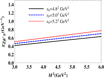
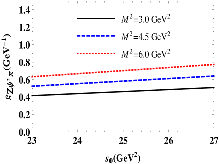
Figure 3: The coupling $g_{Z\psi^{\prime}\pi}$ as a function of the Borel parameter $M^{2}$ at fixed $s_{0}$ (left panel), and as a function of the continuum threshold $s_{0}$ at fixed $M^{2}$ (right panel).

For the strong coupling $g_{Z\psi^{\prime}\pi}$ and width of the corresponding decay $Z\rightarrow\psi^{\prime}\pi$ process numerical computations predict:

$$g_{Z\psi^{\prime}\pi}=(0.58\pm 0.17)\ \mathrm{GeV}^{-1},$$

$$\Gamma(Z\rightarrow\psi^{\prime}\pi)=(129.7\pm 38.4)\ \mathrm{MeV}.$$ (33)

The coupling $g_{ZJ/\psi\pi}$ and width of the decay $Z\to J/\psi\pi$ are found as

$$g_{ZJ/\psi\pi}=(0.24\pm 0.07)\ \mathrm{GeV}^{-1},$$

$$\Gamma(Z\to J/\psi\pi)=(27.4\pm 7.3)\ \mathrm{MeV}.$$ (34)

Our results for all of four strong couplings, as well as the decay width of corresponding processes are collected in Table 3.

Channels	$Z\to\psi^{\prime}\pi$	$Z\to J/\psi\pi$	$Z_{c}\to\psi^{\prime}\pi$	$Z_{c}\to J/\psi\pi$
$g~{}(\mathrm{GeV}^{-1})$	$0.58\pm 0.17$	$0.24\pm 0.07$	$0.29\pm 0.08$	$0.38\pm 0.11$
$\Gamma~{}(\mathrm{MeV})$	$129.7\pm 38.4$	$27.4\pm 7.3$	$7.1\pm 1.9$	$39.9\pm 9.3$

Table 3: The strong coupling $g$ and width $\Gamma$ of the $Z(Z_{c})\to\psi^{\prime}(J/\psi)\pi$ decay channels.

III.2 $Z_{c}(3900),\,Z(4430)\to\eta_{c}^{\prime}\rho;\,\eta_{c}\rho$ decays

The $Z_{c}(3900)$ and $Z(4430)$ may decay also to final states $\eta_{c}\rho$ and $\eta_{c}^{\prime}\rho$. Here we have three decay modes $Z\to\eta_{c}^{\prime}\rho$, $Z\to\eta_{c}\rho$ and $Z_{c}\to\eta_{c}\rho$: the process $Z_{c}\to\eta_{c}^{\prime}\rho$ is forbidden kinematically. An analysis of three decay channels in some points differs from similar studies fulfilled in the previous subsection.

As usual, we consider the correlation function

$$\Pi_{\nu}(p,q)=i\int d^{4}xe^{ipx}\langle\rho(q)|\mathcal{T}\{J^{\eta_{c}}(x)J_{\nu}^{Z\dagger}(0)\}|0\rangle,$$ (35)

where $\eta_{c}\equiv\eta_{c},\ \eta_{c}^{\prime}$, and the current $J^{\eta_{c}}(x)$ is defined as

$$J^{\eta_{c}}(x)=\overline{c}_{i}(x)i\gamma_{5}c_{i}(x).$$

In order to find the hadronic representation of the correlation function we define the matrix elements

$$\langle 0|J^{\eta_{c}}|\eta_{c}(p)\rangle=\frac{f_{\eta_{c}}m_{\eta_{c}}^{2}}{2m_{c}},$$ (36)

with $m_{\eta_{c}}$ and $f_{\eta_{c}}$ being the $\eta_{c}$ ($\eta_{c}^{\prime}$) mesons’ mass and decay constant. The relevant vertices are introduced in the following form

$$\langle\eta_{c}\left(p\right)\rho(q)|Z(p^{\prime})\rangle = g_{Z\eta_{c}\rho}\left[(q\cdot\widetilde{\varepsilon}^{\prime})(p^{\prime}\cdot\varepsilon^{\ast})\right.$$ (37)

$$-\left.(q\cdot p^{\prime})(\varepsilon^{\ast}\cdot\widetilde{\varepsilon}^{\prime})\right],$$

and

$$\langle\eta_{c}\left(p\right)\rho(q)|Z_{c}(p^{\prime})\rangle = g_{Z_{c}\eta_{c}\rho}\left[(q\cdot\varepsilon^{\prime})(p^{\prime}\cdot\varepsilon^{\ast})\right.$$ (38)

$$-\left.(q\cdot p^{\prime})(\varepsilon^{\ast}\cdot\varepsilon^{\prime})\right],$$

with $q$ and $\varepsilon$ being the momentum and polarization vector of the $\rho$-meson, respectively.

Then the calculation of the hadronic representation $\Pi_{\nu}^{\mathrm{Phys}}(p,q)$ is straightforward and yields

$$\Pi_{\nu}^{\mathrm{Phys}}(p,q)=\frac{\langle 0|J^{\eta_{c}}|\eta_{c}\left(p\right)\rangle}{p^{2}-m_{\eta_{c}}^{2}}\langle\eta_{c}\left(p\right)\rho(q)|Z_{c}(p^{\prime})\rangle$$

$$\times\frac{\langle Z_{c}(p^{\prime})|J_{\nu}^{Z}|0\rangle}{p^{\prime 2}-m_{Z_{c}}^{2}}+\sum_{\eta_{c}=\eta_{c},\eta_{c}^{\prime}}\frac{\langle 0|J^{\eta_{c}}|\eta_{c}\left(p\right)\rangle}{p^{2}-m_{\eta_{c}}^{2}}\langle\eta_{c}\left(p\right)\rho(q)|Z(p^{\prime})\rangle$$

$$\times\frac{\langle Z(p^{\prime})|J_{\nu}^{Z}|0\rangle}{p^{\prime 2}-m_{Z}^{2}}+\dots.$$ (39)

Employing the required matrix elements, for the invariant amplitude corresponding to the structure $\sim\epsilon_{\nu}^{\ast}$ in the limit $q\rightarrow 0$ we find

$$\Pi^{\mathrm{Phys}}(p^{2})=\frac{f_{\eta_{c}}f_{Z_{c}}m_{Z_{c}}m_{\eta_{c}}^{2}g_{Z_{c}\eta_{c}\rho}}{4m_{c}\left(p^{2}-\widetilde{m}_{1}^{2}\right)^{2}}(m_{Z_{c}}^{2}-m_{\eta_{c}}^{2})$$

$$+\frac{f_{\eta_{c}}f_{Z}m_{Z}m_{\eta_{c}}^{2}g_{Z\eta_{c}\rho}}{4m_{c}\left(p^{2}-\widetilde{m}_{2}^{2}\right)^{2}}(m_{Z}^{2}-m_{\eta_{c}}^{2})$$

$$+\frac{f_{\eta_{c}^{\prime}}f_{Z}m_{Z}m_{\eta_{c}^{\prime}}^{2}g_{Z\eta_{c}^{\prime}\rho}}{4m_{c}\left(p^{2}-\widetilde{m}_{3}^{2}\right)^{2}}(m_{Z}^{2}-m_{\eta_{c}^{\prime}}^{2})+\ldots,$$ (40)

where the notations $\widetilde{m}_{1}^{2}=(m_{Z_{c}}^{2}+m_{\eta_{c}}^{2})/2$, $\widetilde{m}_{2}^{2}=(m_{Z}^{2}+m_{\eta_{c}}^{2})/2$ and $\widetilde{m}_{3}^{2}=(m_{Z}^{2}+m_{\eta_{c}^{\prime}}^{2})/2$ are introduced.

Computation of the correlation function $\Pi_{\nu}^{\mathrm{QCD}}(p,q)$ using quark propagators yields

$$\Pi_{\nu}^{\mathrm{QCD}}(p,q)=-i\int d^{4}xe^{ipx}\frac{\epsilon\widetilde{\epsilon}}{\sqrt{2}}\left[\gamma_{5}\widetilde{S}_{c}^{ib}(x){}\gamma_{5}\right.$$

$$\left.\times\widetilde{S}_{c}^{ei}(-x){}\gamma_{\nu}+\gamma_{\nu}\widetilde{S}_{c}^{ib}(x){}\gamma_{5}\widetilde{S}_{c}^{ei}(-x){}\gamma_{5}\right]_{\alpha\beta}$$

$$\times\langle\rho(q)|\overline{u}_{\alpha}^{d}(0)d_{\beta}^{a}(0)|0\rangle.$$ (41)

In the $q\to 0$ limit only the matrix elements

$$\langle 0|\overline{u}(0)\gamma_{\mu}d(0)|\rho(p,\lambda)\rangle=\epsilon_{\mu}^{(\lambda)}f_{\rho}m_{\rho},$$ (42)

and

$$\langle 0|\overline{u}(0)g\widetilde{G}_{\mu\nu}\gamma_{\nu}\gamma_{5}d(0)|\rho(p,\lambda)\rangle=f_{\rho}m_{\rho}^{3}\epsilon_{\mu}^{(\lambda)}\zeta_{4\rho},$$ (43)

contribute to the spectral density $\rho^{\mathrm{QCD}}(s)$ Agaev:2016dev . They depend on the mass and decay constant of the $\rho$-meson $m_{\rho}$, $f_{\rho}$, and on $\zeta_{4\rho}$ which normalizes the twist-4 matrix element of the $\rho$-meson Ball:1998ff . The parameter $\zeta_{4\rho}$ was evaluated in the context of QCD sum rule approach at the renormalization scale $\mu=1\,\,{\mathrm{GeV}}$ in Ref. Ball:2007zt and is equal to $\zeta_{4\rho}=0.07\pm 0.03$.

The spectral density $\rho^{\mathrm{QCD}}(s)$ is derived in accordance with known recipes and is given as

$$\rho^{\mathrm{QCD}}(s)=\frac{f_{\rho}m_{\rho}}{8\sqrt{2}}\left[\rho^{\mathrm{pert.}}(s)+\rho^{\mathrm{n.-pert.}}(s)\right],$$ (44)

where

$$\rho^{\mathrm{pert.}}(s)=\frac{\sqrt{s(s-4m_{c}^{2})}}{\pi^{2}}.$$ (45)

The nonperturbative component of $\rho^{\mathrm{QCD}}(s)$ is calculated with dimension-8 accuracy: its explicit form can be found in Appendix.

On order to derive sum rules we use an iterative approach explained in the previous subsection. At the first stage our task is simple. Really, for $s\in(0,\ s_{0})$ there is only one term in the physical side of the sum rule. At this step we evaluate only the ground-state coupling $g_{Z_{c}\eta_{c}\rho}$, therefore can apply the operator $\mathcal{P}$ to clean the physical side of the sum rule form effects of excited states. As a result, we get

$$g_{Z_{c}\eta_{c}\rho} = \frac{4m_{c}}{f_{\eta_{c}}f_{Z_{c}}m_{Z_{c}}m_{\eta_{c}}^{2}(m_{Z_{c}}^{2}-m_{\eta_{c}}^{2})}$$

$$\times\mathcal{P}(M^{2},\widetilde{m}_{1}^{2})\int_{4m_{c}^{2}}^{s_{0}}dse^{-s/M^{2}}\rho^{\mathrm{QCD}}(s).$$

In the domain $s\in(0,\ s_{0}^{\ast})$ all terms in Eq. (40) become active, and we obtain the expression containing two remaining unknown couplings. Because excited terms enter to this expression explicitly and our aim is to find corresponding couplings, we do not apply the operator $\mathcal{P}$. The system of equations can be completed by using the operator $d/d(-1/M^{2})$ to both sides of this expression which leads the second equality. Solutions of the obtained equations are sum rules for the couplings $g_{Z\eta_{c}}\rho$ and $g_{Z\eta_{c}}^{\prime}\rho$. The width of the decays $Z\rightarrow\eta_{c}\rho$, $Z\rightarrow\eta_{c}^{\prime}\rho$ and $Z_{c}\rightarrow\eta_{c}\rho$ can be calculated by means of Eq. (31) with replacements $m_{\pi}\rightarrow m_{\eta_{c}}(m_{\eta_{c}^{\prime}})$ and $m_{\psi}\rightarrow m_{\rho}$.

For the coupling $g_{Z_{c}\eta_{c}\rho}$ and width of the decay $Z_{c}\rightarrow\eta_{c}\rho$ we get

$$g_{Z_{c}\eta_{c}\rho}=(1.28\pm 0.32)\ \mathrm{GeV}^{-1},$$

$$\Gamma(Z_{c}\rightarrow\eta_{c}\rho)=(20.28\pm 5.17)\ \mathrm{MeV}.$$ (46)

For the strong couplings $g_{Z\eta_{c}^{\prime}\rho}$ and $g_{Z\eta_{c}\rho}$, and width of the processes $Z\to\eta_{c}^{\prime}\rho$ and $Z\to\eta_{c}\rho$ we find

$$g_{Z\eta_{c}^{\prime}\rho}=(0.81\pm 0.21)\ \mathrm{GeV}^{-1},$$

$$\Gamma(Z\to\eta_{c}^{\prime}\rho)=(1.01\pm 0.28)\ \mathrm{MeV},$$ (47)

and

$$g_{Z\eta_{c}\rho}=(0.48\pm 0.13)\ \mathrm{GeV}^{-1},$$

$$\Gamma(Z\to\eta_{c}\rho)=(11.57\pm 3.04)\ \mathrm{MeV}.$$ (48)

The decays $Z_{c}\to J/\psi\pi$ and $Z_{c}\to\eta_{c}\rho$ were considered in our previous work Agaev:2016dev using QCD sum rules on light-cone and diquark-antidiquark interpolating current. In Table 4 the partial decay width of these channels obtained in Ref. Agaev:2016dev are compared with predictions of the present investigation. As is seen, they do not differ considerably from each other: it is remarkable, that iterative scheme adopted in this work lead to almost identical to Ref. Agaev:2016dev predictions, which may be considered as serious consistency-check of the employed approach. The small discrepancies between two sets of predictions can be attributed to accuracy of the spectral densities, which in the present work have been found by taking into account condensates up to eight dimensions, whereas in Ref. Agaev:2016dev $\rho_{\pi}^{\mathrm{QCD}}(s)$ and $\rho_{\rho}^{\mathrm{QCD}}(s)$ contained only perturbative terms. It is worth noting that, in the present work we have evaluated the partial width of the $Z_{c}\to\psi^{\prime}\pi$ mode, which was not considered in Ref. Agaev:2016dev .

Our results for the decays of the $Z(4430)$ resonance are collected in Table 5. As is seen, $Z$ dominantly decays through $Z\to\psi^{\prime}\pi$ channel. The sum of predictions for the channels $Z\to\psi^{\prime}\pi$ and $Z\to J/\psi\pi$ $(157.1\pm 39.1)\ {\mathrm{MeV}}$ agrees with LHCb measurements (see, Eq. (1)) staying below the upper limit of experimental data $\sim 212\ {\mathrm{MeV}}$. Unfortunately, an experimental information on the decay width $\Gamma(Z\to J/\psi\pi)$ is restricted by Belle report on product of branching fractions $\mathcal{B}(\bar{B}^{0}\to K^{-}Z(4430)^{+})\mathcal{B}(Z(4430)^{+}\to J/\psi\pi)=(5.4^{+4.0}_{-1.0}{}^{+1.1}_{-0.9})\cdot 10^{-6}$. It is possible, by invoking a similar experimental measurements for $\psi^{\prime}$ to estimate a ratio

$$R_{Z}=\Gamma(Z\to\psi^{\prime}\pi)/\Gamma(Z\to J/\psi\pi),$$ (49)

which actually was done in Ref. Goerke:2016hxf . But we are not going to make far-reaching conclusions from similar estimates: From our point of view, in the lack of direct measurements of $\Gamma(Z\to J/\psi\pi)$, the best what can be done is calculation of theoretical prediction for $R_{Z}$, which equals in our case to $R_{Z}=4.73\pm 1.88$.

	$\Gamma(Z_{c}\to J/\psi\pi)$	$\Gamma(Z_{c}\to\psi^{\prime}\pi)$	$\Gamma(Z_{c}\to\eta_{c}\rho)$
	$(\mathrm{MeV})$	$(\mathrm{MeV})$	$(\mathrm{MeV})$
This work	$39.9\pm 9.3$	$7.1\pm 1.9$	$20.3\pm 5.2$
Agaev:2016dev	$41.9\pm 9.4$	$-$	$23.8\pm 4.9$
Dias:2013xfa	$29.1\pm 8.2$	$-$	$27.5\pm 8.5$
Goerke:2016hxf A	$27.9^{+6.3}_{-5.0}$	$-$	$35.7^{+6.3}_{-5.2}$
Goerke:2016hxf B	$1.8\pm 0.3$	$-$	$3.2^{+0.5}_{-0.4}$
Dong:2013iqa	$10.43-23.89$	$1.28-2.94$	$-$

Table 4: Theoretical results for some of the $Z_{c}(3900)$ resonance’s decay modes.

	$\Gamma(Z\to J/\psi\pi)$	$\Gamma(Z\to\psi^{\prime}\pi)$	$\Gamma(Z\to\eta_{c}\rho)$	$\Gamma(Z\to\eta_{c}^{\prime}\rho)$
	$(\mathrm{MeV})$	$(\mathrm{MeV})$	$(\mathrm{MeV})$	$(\mathrm{MeV})$
Th. w.	$27.4\pm 7.3$	$129.7\pm 38.4$	$11.6\pm 3.0$	$1.0\pm 0.3$
Goerke:2016hxf	$26.9$	$120.6$	$-$	$-$

Table 5: The same as in Table 4, but for the $Z(4430)$ state.

IV Summary and Concluding notes

The decays of $Z$ and $Z_{c}$ resonances were previously investigated in Ref. Goerke:2016hxf ; Dias:2013xfa ; Dong:2013iqa : some of their results are shown in Tables 4 and 5. In Ref. Dias:2013xfa using the three-point sum rule method and diquark-antidiquark interpolating current authors calculated partial decay width of the channels $Z_{c}\to J/\psi\pi$, $Z_{c}\to\eta_{c}\rho$, $Z_{c}\to\bar{D}^{0}D^{\star}$ and $Z_{c}\to\bar{D}^{\star 0}D$ . Results for two first modes can be found in Table 4.

Within the covariant quark model decays of the $Z_{c}(3900)$ state were analyzed in Ref. Goerke:2016hxf , where it was considered both as a diqaurk-antidiquak and molecule-type tetraquarks. Thus, by treating $Z_{c}$ as a four-quark system with diquark-antidiquark composition and using a size parameter $\Lambda_{Z_{c}}=2.25\pm 0.10\ \mathrm{GeV}$ in their model (model A) authors evaluated width of the decays $Z_{c}\to J/\psi\pi$, $Z_{c}\to\eta_{c}\rho$ (see, Table 4). Assuming a molecular-type structure for $Z_{c}(3900)$ and choosing $\Lambda_{Z_{c}}=3.3\pm 0.1\ \mathrm{GeV}$ (model B) the same decay widths were calculated in Ref. Goerke:2016hxf : obtained predictions are shown in Table 4, too.

The decays of $Z_{c}(3900)$ state in the framework of a phenomenological Lagrangian approach were considered in Ref. Dong:2013iqa . The $Z_{c}$ state there was treated as a hadronic molecule composed of $\bar{D}D^{\star}$ and $\bar{D}^{\star}D$. For a binding energy of the hadronic molecule $\epsilon=20\ \mathrm{MeV}$ authors found the width of different decay channels, some of which are demonstrated in Table 4.

Decays of the $Z(4430)$ resonance to $J/\psi\pi$ and $\psi^{\prime}\pi$ in the context of the diquark-antidiquark model were studied in Ref. Goerke:2016hxf . Predictions for the partial width of these decays (see, Table 5) obtained at $\Lambda_{Z(4430)}=2.4\ \mathrm{GeV}$, as well as estimates for $\Gamma(Z\to J/\psi\pi)+\Gamma(Z\to\psi^{\prime}\pi)=147.5\ \mathrm{MeV}$ and for the ratio $R_{Z}=4.48$ are close to our results.

We have tested a suggestion on $Z(4430)$ resonance as first radially excited state of the diquark-antidiquark state $Z_{c}(3900)$. For the masses and total widths of the $Z_{c}(3900)$ and $Z(4430)$ resonances we have found: $m_{Z_{c}}=3901^{+125}_{-148}\ \mathrm{MeV}$, $\Gamma_{Z_{c}}=(67.3\pm 10.8)\ \mathrm{MeV}$, and $m_{Z}=4452^{+182}_{-228}\ \mathrm{MeV}$, $\Gamma_{Z}=(169.7\pm 39.2)\ \mathrm{MeV}$. Results of the present work seem support assumption on excited nature of the $Z(4430)$ resonance. But there are problems to be addressed before drawing strong conclusions. Namely, theoretical investigations of other decay channels of $Z_{c}(3900)$ and $Z(4430)$ states has to be carried out in order to obtain more accurate predictions for their total widths. Experimental studies of the $Z(4430)$ resonance’s decay channels, especially a direct measurement of $\Gamma(Z\to J/\psi\pi)$ may help in clarifying its nature as a radial excitation of $Z_{c}(3900)$ state.

Appendix A The quark propagators and spectral densities

The light and heavy quark propagators are necessary to find QCD side of the correlation functions in both mass, current and strong couplings’ calculations. In the present work we employ the $q$- quark propagator $S_{q}^{ab}(x)$, which is given by the following formula

$$S_{q}^{ab}(x)=i\delta_{ab}\frac{\not{x}}{2\pi^{2}x^{4}}-\delta_{ab}\frac{m_{q}}{4\pi^{2}x^{2}}-\delta_{ab}\frac{\langle\overline{q}q\rangle}{12}$$

$$+i\delta_{ab}\frac{\not{x}m_{q}\langle\overline{q}q\rangle}{48}-\delta_{ab}\frac{x^{2}}{192}\langle\overline{q}g_{s}\sigma Gq\rangle+i\delta_{ab}\frac{x^{2}\not{x}m_{q}}{1152}$$

$$\times\langle\overline{q}g_{s}\sigma Gq\rangle-i\frac{g_{s}G_{ab}^{\alpha\beta}}{32\pi^{2}x^{2}}\left[\not{x}{\sigma_{\alpha\beta}+\sigma_{\alpha\beta}}\not{x}\right]$$

$$-i\delta_{ab}\frac{x^{2}\not{x}g_{s}^{2}\langle\overline{q}q\rangle^{2}}{7776}-\delta_{ab}\frac{x^{4}\langle\overline{q}q\rangle\langle g_{s}^{2}G^{2}\rangle}{27648}+\ldots$$ (A.50)

For the $c$-quark propagator $S_{c}^{ab}(x)$ we use the well-known expression

$$S_{c}^{ab}(x)=i\int\frac{d^{4}k}{(2\pi)^{4}}e^{-ikx}\Bigg{\{}\frac{\delta_{ab}\left({\not{k}}+m_{c}\right)}{k^{2}-m_{c}^{2}}$$

$$-\frac{g_{s}G_{ab}^{\alpha\beta}}{4}\frac{\sigma_{\alpha\beta}\left({\not{k}}+m_{c}\right)+\left({\not{k}}+m_{c}\right)\sigma_{\alpha\beta}}{(k^{2}-m_{c}^{2})^{2}}$$

$$+\frac{g_{s}^{2}G^{2}}{12}\delta_{ab}m_{c}\frac{k^{2}+m_{c}{\not{k}}}{(k^{2}-m_{c}^{2})^{4}}+\frac{g_{s}^{3}G^{3}}{48}\delta_{ab}\frac{\left({\not{k}}+m_{c}\right)}{(k^{2}-m_{c}^{2})^{6}}$$

$$\times\left[{\not{k}}\left(k^{2}-3m_{c}^{2}\right)+2m_{c}\left(2k^{2}-m_{c}^{2}\right)\right]\left({\not{k}}+m_{c}\right)+\ldots\Bigg{\}}.$$

In Eqs. (A.50) and (LABEL:eq:Qprop) we adopt the notations

$$G_{ab}^{\alpha\beta}=G_{A}^{\alpha\beta}t_{ab}^{A},\,\,~{}~{}G^{2}=G_{\alpha\beta}^{A}G_{\alpha\beta}^{A},$$

$$G^{3}=\,\,f^{ABC}G_{\mu\nu}^{A}G_{\nu\delta}^{B}G_{\delta\mu}^{C},$$ (A.52)

with $a,\,b=1,2,3$ being the color indices, and $A,B,C=1,\,2\,\ldots 8$  . In Eq. (A.52) $t^{A}=\lambda^{A}/2$, $\lambda^{A}$ are the Gell-Mann matrices, and the gluon field strength tensor $G_{\alpha\beta}^{A}\equiv G_{\alpha\beta}^{A}(0)$ is fixed at $x=0$.

The nonperturbative part of the spectral density Eq. (26) is determined by the formula

$$\rho^{\mathrm{n.-pert.}}(s)=\Big{\langle}\frac{\alpha_{s}G^{2}}{\pi}\Big{\rangle}m_{c}^{2}\int_{0}^{1}f_{1}(z,s)dz$$

$$+\Big{\langle}g_{s}^{3}G^{3}\Big{\rangle}\int_{0}^{1}f_{2}(z,s)dz$$

$$+\Big{\langle}\frac{\alpha_{s}G^{2}}{\pi}\Big{\rangle}^{2}m_{c}^{2}\int_{0}^{1}f_{3}(z,s)dz.$$ (A.53)

In Eq. (A.53) the functions $f_{1}(z,s),\ f_{2}(z,s)$ and $f_{3}(z,s)$ have the explicit forms:

$$f_{1}(z,s)=\frac{1}{6r^{2}}\left\{-\left(1+3r\right)\delta^{\prime}(s-\Phi)\right.$$

$$\left.+s(1+2r)\delta^{(2)}(s-\Phi)\right\},$$ (A.54)

$$f_{2}(z,s)=\frac{1}{15\cdot 2^{7}\pi^{2}r^{5}}\left\{2r^{2}\left[-9m_{c}^{2}\left(1+5r(1+r)\right)\right.\right.$$

$$\left.+2sr(3+r(19+27r))\right]\delta^{(2)}(s-\Phi)+r\left[s^{2}r^{3}(8+27r)\right.$$

$$\left.m_{c}^{4}(1+5r(1+r))+6m_{c}^{2}sr(3+r(11+3r))\right]\delta^{(3)}(s-\Phi)$$

$$+\left[s^{3}r^{5}+6m_{c}^{2}s^{2}r^{3}(1+2r)+2m_{c}^{6}(1+5r(1+r))\right.$$

$$\left.\left.-m_{c}^{4}sr(7+r(31+23r))\right]\delta^{(4)}(s-\Phi)\right\},$$ (A.55)

and

$$f_{3}(z,s)=\frac{\pi^{2}}{108r^{2}}\left[6r\delta^{(3)}(s-\Phi)-(m_{c}^{2}-2s-6sr)\right.$$

$$\left.\times\delta^{(4)}(s-\Phi)-s(m_{c}^{2}-rs)\delta^{(5)}(s-\Phi)\right],$$ (A.56)

where we use the notations

$$\ r=z(z-1),\ \ \Phi=\frac{m_{c}^{2}}{z(1-z)}.$$ (A.57)

In the expressions above the Dirac delta function $\ \delta^{(n)}(s-\Phi)$ is defined as

$$\delta^{(n)}(s-\Phi)=\frac{d^{n}}{ds^{n}}\delta(s-\Phi).$$ (A.58)

The nonperturbative component of $\rho^{\mathrm{QCD}}(s)$ defined by Eq. (44) is given by the formulas:

$$\rho^{\mathrm{n.-pert.}}(s)=\frac{\zeta_{4\rho}m_{\rho}^{2}}{s}+\Big{\langle}\frac{\alpha_{s}G^{2}}{\pi}\Big{\rangle}m_{c}^{2}\int_{0}^{1}\widetilde{f}_{1}(z,s)dz$$

$$+\Big{\langle}g_{s}^{3}G^{3}\Big{\rangle}\int_{0}^{1}\widetilde{f}_{2}(z,s)dz$$

$$+\Big{\langle}\frac{\alpha_{s}G^{2}}{\pi}\Big{\rangle}^{2}m_{c}^{2}\int_{0}^{1}\widetilde{f}_{3}(z,s)dz,$$ (A.59)

where

$$\widetilde{f}_{1}(z,s)=-\frac{s(1+2r)}{9}\delta^{(2)}(s-\Phi),$$ (A.60)

$$\widetilde{f}_{2}(z,s)=\frac{1}{45\cdot 2^{6}\pi^{2}r^{5}}\left\{12sr^{3}\left[1+r(7+11r)\right]\right.$$

$$\times\delta^{(2)}(s-\Phi)+2r\left[2s^{2}r^{3}(2+7r)-3m_{c}^{4}\left(1\right.\right.$$

$$\left.\left.+5r(1+r)\right)+9m_{c}^{2}sr\left(1+2r(2+z)\right)\right]\delta^{(3)}(s-\Phi)$$

$$+\left[s^{3}r^{5}+6m_{c}^{2}s^{2}r^{3}(1+2r)+2m_{c}^{6}\left(1+5r(1+r)\right)\right.$$

$$\left.\left.-m_{c}^{4}sr\left(7+r(31+23r)\right)\right]\delta^{(4)}(s-\Phi)\right\},$$ (A.61)

and

$$\widetilde{f}_{3}(z,s)=\frac{1}{3^{4}\cdot 2}\left\{-6r\delta^{(3)}(s-\Phi)+2\left[m_{c}^{2}-s(1+3r)\right]\right.$$

$$\left.\times\delta^{(4)}(s-\Phi)+s(m_{c}^{2}-sr)\delta^{(5)}(s-\Phi)\right\}.$$ (A.62)

References

- (1) S. K. Choi et al. [Belle Collaboration], Phys. Rev. Lett. 100, 142001 (2008).
- (2) R. Mizuk et al. [Belle Collaboration], Phys. Rev. D 80, 031104 (2009).
- (3) K. Chilikin et al. [Belle Collaboration], Phys. Rev. D 88, 074026 (2013).
- (4) K. Chilikin et al. [Belle Collaboration], Phys. Rev. D 90, 112009 (2014).
- (5) R. Aaij et al. [LHCb Collaboration], Phys. Rev. Lett. 112, 222002 (2014).
- (6) R. Aaij et al. [LHCb Collaboration], Phys. Rev. D 92, 112009 (2015)
- (7) M. Ablikim et al. [BESIII Collaboration], Phys. Rev. Lett. 110, 252001 (2013).
- (8) Z. Q. Liu et al. [Belle Collaboration], Phys. Rev. Lett. 110, 252002 (2013).
- (9) T. Xiao, S. Dobbs, A. Tomaradze and K. K. Seth, Phys. Lett. B 727, 366 (2013).
- (10) M. Ablikim et al. [BESIII Collaboration], Phys. Rev. Lett. 115, 112003 (2015).
- (11) H. X. Chen, W. Chen, X. Liu and S. L. Zhu, Phys. Rept. 639, 1 (2016).
- (12) A. Esposito, A. Pilloni and A. D. Polosa, Phys. Rept. 668, 1 (2016).
- (13) X. H. Liu, Q. Zhao and F. E. Close, Phys. Rev. D 77, 094005 (2008).
- (14) D. Ebert, R. N. Faustov and V. O. Galkin, Eur. Phys. J. C 58, 399 (2008).
- (15) M. E. Bracco, S. H. Lee, M. Nielsen and R. Rodrigues da Silva, Phys. Lett. B 671, 240 (2009).
- (16) L. Maiani, A. D. Polosa and V. Riquer, New J. Phys. 10, 073004 (2008).
- (17) Z. G. Wang, Eur. Phys. J. C 70, 139 (2010).
- (18) L. Maiani, F. Piccinini, A. D. Polosa and V. Riquer, Phys. Rev. D 89, 114010 (2014).
- (19) Z. G. Wang, Commun. Theor. Phys. 63, 325 (2015).
- (20) S. H. Lee, A. Mihara, F. S. Navarra and M. Nielsen, Phys. Lett. B 661, 28 (2008).
- (21) X. Liu, Y. R. Liu, W. Z. Deng and S. L. Zhu, Phys. Rev. D 77, 094015 (2008).
- (22) E. Braaten and M. Lu, Phys. Rev. D 79, 051503 (2009).
- (23) T. Branz, T. Gutsche and V. E. Lyubovitskij, Phys. Rev. D 82, 054025 (2010).
- (24) F. Goerke, T. Gutsche, M. A. Ivanov, J. G. Korner, V. E. Lyubovitskij and P. Santorelli, Phys. Rev. D 94, 094017 (2016).
- (25) J. L. Rosner, Phys. Rev. D 76, 114002 (2007).
- (26) S. Dubynskiy and M. B. Voloshin, Phys. Lett. B 666, 344 (2008).
- (27) J. M. Dias, F. S. Navarra, M. Nielsen and C. M. Zanetti, Phys. Rev. D 88, 016004 (2013).
- (28) Z. G. Wang and T. Huang, Phys. Rev. D 89, 054019 (2014).
- (29) C. Deng, J. Ping and F. Wang, Phys. Rev. D 90, 054009 (2014).
- (30) S. S. Agaev, K. Azizi and H. Sundu, Phys. Rev. D 93, 074002 (2016).
- (31) Z. G. Wang and T. Huang, Phys. J. C 74, 2891 (2014).
- (32) E. Wilbring, H.-W. Hammer and U.-G. Mei?ner, Phys. Lett. B 726, 326 (2013).
- (33) Y. Dong, A. Faessler, T. Gutsche and V. E. Lyubovitskij, Phys. Rev. D 88, 014030 (2013).
- (34) H. W. Ke, Z. T. Wei and X. Q. Li, Eur. Phys. J. C 73, 2561 (2013).
- (35) T. Gutsche, M. Kesenheimer and V. E. Lyubovitskij, Phys. Rev. D 90, 094013 (2014).
- (36) A. Esposito, A. L. Guerrieri and A. Pilloni, Phys. Lett. B 746, 194 (2015).
- (37) D. Y. Chen and Y. B. Dong, Phys. Rev. D 93, 014003 (2016).
- (38) Q. R. Gong, Z. H. Guo, C. Meng, G. Y. Tang, Y. F. Wang and H. Q. Zheng, Phys. Rev. D 94, 114019 (2016).
- (39) H. W. Ke and X. Q. Li, Eur. Phys. J. C 76, 334 (2016).
- (40) E. S. Swanson, Phys. Rev. D 91, 034009 (2015).
- (41) Y. Ikeda et al. [HAL QCD Collaboration], Phys. Rev. Lett. 117, 242001 (2016).
- (42) S. S. Agaev, K. Azizi and H. Sundu, arXiv:1703.10323 [hep-ph] (Phys. Rev. D, to be published).
- (43) V. M. Belyaev, V. M. Braun, A. Khodjamirian and R. Ruckl, Phys. Rev. D 51, 6177 (1995).
- (44) B. L. Ioffe and A. V. Smilga, Nucl. Phys. B 232, 109 (1984).
- (45) C. Patrignani, Chin. Phys. C 40, 100001 (2016).
- (46) H. Negash and S. Bhatnagar, Int. J. Mod. Phys. E 25, 1650059 (2016).
- (47) P. Ball and V. M. Braun, Nucl. Phys. B 543, 201 (1999).
- (48) P. Ball, V. M. Braun and A. Lenz, JHEP 0708, 090 (2007).