$Z^{+}(4430)$ as a $D_{1}^{\prime}{D}^{*}$ ($D_{1}{D}^{*}$) molecular state

Abstract

We reexamine whether $Z^{+}(4430)$ could be a $D_{1}^{\prime}-{D}^{*}$ or $D_{1}-{D}^{*}$ molecular state after considering both the pion and $\sigma$ meson exchange potentials and introducing the form factor to take into account the structure effect of the interaction vertex. Our numerical analysis with Matlab package MATSLISE indicates the contribution from the sigma meson exchange is small for the $D_{1}^{\prime}-{D}^{*}$ system and significant for the $D_{1}-{D}^{*}$ system. The S-wave $D_{1}-\bar{D}^{*}$ molecular state with only $J^{P}=0^{-}$ and $D_{1}^{\prime}-{D}^{*}$ molecular states with $J^{P}=0^{-},1^{-},2^{-}$ may exist with reasonable parameters. One should investigate whether the broad width of $D_{1}^{\prime}$ disfavors the possible formation of molecular states in the future. The bottom analog $Z_{B}$ of $Z^{+}(4430)$ has a larger binding energy, which may be searched at Tevatron and LHC. Experimental measurement of the quantum number of $Z^{+}(4430)$ may help uncover its underlying structure.

I introduction

Recently Belle collaboration observed one very exotic resonance $Z^{+}(4430)$ in the $\pi^{+}\psi^{\prime}$ invariant mass spectrum in the exclusive $B\to K\pi^{+}\psi^{\prime}$ decays Belle-4430 . Its mass and width are

$$M=4433\pm 4(\mathrm{stat})\pm 1(\mathrm{syst})\;\;\mathrm{MeV}$$

and

$$\Gamma=44^{+17}_{-13}(\mathrm{stat})^{+30}_{-11}(\mathrm{syst})\;\;\mathrm{MeV}.$$

This resonance appears as an excellent candidate of either the multiquark state or the molecular state and has stimulated many theoretical investigations xiangliu ; rosner ; Meng ; Bugg ; cky ; maiani ; Gershtein ; Qiao ; qsr ; LiY ; ding ; braaten ; LiuXH ; voloshin ; polosa ; godfrey . A concise review of the theoretical status of $Z^{+}(4430)$ can be found in Ref. xiangliu . Thereafter Ding studied $Z^{+}(4430)$ using the approach of effective Lagrangian and predicted a $B^{*}B_{1}$ bound state with mass 11048.6 MeV ding . Later Braaten and Lu studied the line shapes of $Z^{+}(4430)$ braaten .

In our previous work xiangliu , we explored whether $Z^{+}(4430)$ could be a loosely bound S-wave molecular state of $D^{*}$ and $\bar{D}_{1}^{\prime}$ (or $\bar{D}_{1}$) with $J^{P}=0^{-},1^{-},2^{-}$. We considered the one-pion exchange potential only and did not introduce the form factor in the scattering matrix elements in the derivation of the potential. Instead of solving the Schrodinger equation numerically, we employed some simple trial wave functions and the variation method to study whether a shallow bound state exists. We found that the interaction from the one pion exchange alone is not strong enough to bind the pair of charmed mesons with realistic coupling constants. Other dynamics is necessary if $Z^{+}(4430)$ is a molecular state.

The one pion exchange potential alone does not bind neutron and proton to form the deuteron in nuclear physics either. The strong attractive force in the intermediate range is required in order to bind the deuteron, which is modelled by the sigma meson exchange. Meanwhile hadrons are not point-like objects. The cutoff should be introduced to describe the structure effect of the interaction vertex. With the above considerations, we have reexamined the $D\bar{D}^{*}$ molecule picture for $X(3872)$ after taking into account both the pion and sigma meson exchange. It turns out that the sigma meson exchange potential is repulsive and numerically important 3872-liu . One may wonder whether the similar mechanism plays a role in the case of $Z^{+}(4430)$. Therefore we will make a comprehensive study whether $Z^{+}(4430)$ is the molecular state.

This work is organized as follows. We present the effective Lagrangian relevant to calculate the $\pi$ and $\sigma$ exchange potentials for $Z^{+}(4430)$ in Section II. We present the detail of the derivation of the potential in Section III. We discuss the behavior of the potential in Section IV. We make numerical analysis in Section V. We discuss the bottom analog of $Z^{+}(4430)$ in Section VI. We discuss the cutoff dependence in Section VII. The last section is the conclusion.

II The effective Lagrangian and coupling constants

In order to derive the $\pi$ and $\sigma$ exchange potentials, we collect the relevant effective Lagrangian in this section. The Lagrangian for the interaction of $\pi$ and charmed mesons is constructed in chiral symmetry and heavy quark limit falk ; casalbuoni

$$\mathcal{L}_{\pi} = ig{\rm Tr}[H_{b}{A}\!\!\!/_{ba}\gamma_{5}\bar{H}_{a}]+ig^{\prime}{\rm Tr}[S_{b}{A}\!\!\!/_{ba}\gamma_{5}\bar{S}_{a}]+ig^{\prime\prime}{\rm Tr}[T_{\mu b}A\!\!\!/_{ba}\gamma_{5}\bar{T}_{a}^{\mu}]+ih{\rm Tr}[S_{b}{A}\!\!\!/_{ba}\gamma_{5}\bar{H}_{a}]$$ (1)

$$+i\frac{h_{1}}{\Lambda_{\chi}}{\rm Tr}[T_{b}^{\mu}(D_{\mu}{A}\!\!\!/)_{ba}\gamma_{5}\bar{H}_{a}]+i\frac{h_{2}}{\Lambda_{\chi}}{\rm Tr}[T_{b}^{\mu}(D\!\!\!\!/A_{\mu})_{ba}\gamma_{5}\bar{H}_{a}]+h.c.$$

where the fields $H$, $S$ and $T$ are defined in terms of the $(0^{-},1^{-})$, $(0^{+},1^{+})$, $(1^{+},2^{+})$ doublets respectively

$$H_{a} = \frac{1+\not v}{2}[P_{a}^{*\mu}\gamma_{\mu}-P_{a}\gamma_{5}],$$ (2)

$$S_{a} = \frac{1+\not v}{2}[P_{1a}^{{}^{\prime}\mu}\gamma_{\mu}\gamma_{5}-P_{0a}^{*}],$$ (3)

$$T_{a}^{\mu} = \frac{1+\not v}{2}\Big{\{}P^{*\mu\nu}_{2a}\gamma_{\nu}-\sqrt{\frac{3}{2}}P_{1a}^{\nu}\gamma_{5}[g_{\nu}^{\mu}-\frac{1}{3}\gamma_{\nu}(\gamma^{\mu}-v^{\mu})]\Big{\}}.$$ (4)

Here the axial vector field $A_{ab}^{\mu}$ is defined as

$$A_{ab}^{\mu}=\frac{1}{2}(\xi^{{\dagger}}\partial^{\mu}\xi-\xi\partial^{\mu}\xi^{{\dagger}})_{ab}=\frac{i}{f_{\pi}}\partial^{\mu}\mathcal{M}_{ab}+\cdots$$

with $\xi=\exp(i\mathcal{M}/f_{\pi})$, $f_{\pi}=132$ MeV and

$$\mathcal{M} = \left(\begin{array}[]{ccc}\frac{\pi^{0}}{\sqrt{2}}+\frac{\eta}{\sqrt{6}}&\pi^{+}&K^{+}\\ \pi^{-}&-\frac{\pi^{0}}{\sqrt{2}}+\frac{\eta}{\sqrt{6}}&K^{0}\\ K^{-}&\bar{K}^{0}&-\frac{2\eta}{\sqrt{6}}\end{array}\right).$$ (8)

In Eq. (1), the coupling constants were estimated in the quark model falk ,

$$g=g_{A},\quad g^{\prime}=g_{A}/3,\quad g^{\prime\prime}=g_{A}$$ (9)

with $g_{A}=0.75$. A different set of coupling constants can be found in Ref. behill . With our notation, we get the following relations

$$g=g_{A}^{\prime},\quad g^{\prime}=-g_{A}^{\prime},\quad h=\frac{1}{2}G_{A}$$ (10)

with $G_{A}\approx 1$ and $g_{A}^{\prime}=0.6$ behill . In fact, the coupling constant $g_{A}$ was studied in many theoretical approaches such as QCD sum rules QSR ; QSR-1 ; QSR-2 ; QSR-3 . In this work we use the experimental value $g_{A}=0.59\pm 0.07\pm 0.01$ extracted from the width of $D^{*}$ isoda . With the available experimental information, Casalbuoni and collaborators extracted $h=0.56\pm 0.28$ and $h^{\prime}=(h_{1}+h_{2})/\Lambda_{\chi}=0.55$ GeV^-1 casalbuoni . The signs of $g,\;g^{\prime}\;g^{\prime\prime}$ are not determined although their absolute values are known.

The interaction Lagrangian related to the $\sigma$ meson can be written as

$$\mathcal{L}_{\sigma} = g_{\sigma}{\rm Tr}[H\sigma\overline{H}]+g^{\prime}_{\sigma}{\rm Tr}[S\sigma\overline{S}]+g^{{}^{\prime\prime}}_{\sigma}{\rm Tr}[T^{\mu}\sigma\overline{T}_{\mu}]$$ (11)

$$+\frac{h_{\sigma}}{f_{\pi}}{\rm Tr}[S(\partial_{\mu}\sigma)\gamma^{\mu}\overline{H}]+\frac{h^{\prime}_{\sigma}}{f_{\pi}}{\rm Tr}[T^{\mu}(\partial_{\mu}\sigma)\overline{H}]+h.c.$$

In order to estimate the values of the coupling constants, we compare the above Lagrangian with that in Ref. behill and get

$$g_{\sigma}=-\frac{1}{2\sqrt{6}}g_{\pi},\quad g_{\sigma}^{\prime}=-\frac{1}{2\sqrt{6}}g_{\pi},\quad h_{\sigma}=\frac{1}{\sqrt{3}}g_{A}^{\prime},$$ (12)

where $g_{\pi}=3.73$. When performing numerical analysis, we take $g_{\sigma}^{\prime\prime}=g_{\sigma}$ and $h_{\sigma}^{\prime}=h_{\sigma}$ approximately.

III Derivation of the pion and sigma exchange potential

If $Z^{+}(4430)$ is a molecular state of $D_{1}^{\prime}-D^{*}$ or $D_{1}-D^{*}$, the flavor wavefunction of $Z^{+}(4430)$ reads xiangliu ,

$$|Z^{+}(4430)\rangle=\frac{1}{\sqrt{2}}\Big{[}|\bar{D}_{1}^{{}^{\prime}0}D^{*+}\rangle+|\bar{D}^{*0}D_{1}^{{}^{\prime}+}\rangle\Big{]}$$ (13)

or

$$|Z^{+}(4430)\rangle=\frac{1}{\sqrt{2}}\Big{[}|\bar{D}_{1}^{0}D^{*+}\rangle+|\bar{D}^{*0}D_{1}^{+}\rangle\Big{]}.$$ (14)

Here $D_{1}^{\prime}$ and $D_{1}$ with quantum number $J^{P}=1^{+}$ belong to $(0^{+},1^{+})$ and $(1^{+},2^{+})$ doublet respectively in the heavy quark limit.

To derive the effective potentials, we follow the same procedure as in Ref. xiangliu . Firstly we write out the elastic scattering amplitudes of the direct process $A(B)\to A(B)$ and crossed channel $A(B)\to B(A)$, where $A$ and $B$ denote $D_{1}^{(^{\prime})}$ and $D^{*}$. Secondly, we impose the constraint that initial states and final states should have the same angular momentum. Thirdly, we average the potentials obtained with Breit approximation in the momentum space. Finally we perform Fourier transformation to derive the potentials in the coordinate space. For the scattering between $D^{\ast}$ and $D_{1}^{\prime}$ ($D_{1}$), both the pion and sigma meson exchange are allowed in both direct and crossed processes.

We introduce the form factor (FF) in every interaction vertex to compensate the off-shell effects of the exchanged mesons when writing out the scattering amplitude, which differs from Ref. xiangliu . One adopts the dipole type FF Tornqvist ; FF

$$F(q)=\Big{(}\frac{\Lambda^{2}-m^{2}}{\Lambda^{2}-q^{2}}\Big{)}^{2}\;.$$ (15)

The phenomenological parameter $\Lambda$ is near 1 GeV. $q$ denotes the four-momentum of the exchange meson. It is observed that as $q^{2}\to 0$ it becomes a constant and if $\Lambda\gg M$, it turns to be unity. In the case, as the distance is infinitely large, the vertex looks like a perfect point, so the form factor is simply 1 or a constant. Whereas, as $q^{2}\rightarrow\infty$, the form factor approaches to zero, namely, in this situation, the distance becomes very small, the inner structure (quark, gluon degrees of freedom) would manifest itself and the whole picture of hadron interaction is no longer valid, so the form factor is zero which cuts off the end effects FF .

For the direct scattering channel, $q_{0}$ is a small value. In the heavy quark limit we approximately take $q_{0}=0$. Thus it is reasonable to approximate $q^{2}$ as $-\mathbf{q}^{2}$. However, for the crossed diagram, we can not ignore the contribution from $q_{0}$ due to $q_{0}=M_{D_{1}}-M_{D^{*}}\approx 410$ MeV, which is about three times of the pion mass. The principal integration is a good approach to solve the problem when $q_{0}$ is larger than the mass of exchanging meson.

Since we only consider S-wave bound states between $D_{1}^{{}^{\prime}}(D_{1})$ and $D^{*}$, there are five independent parts related to the potentials of $D_{1}^{{}^{\prime}}(D_{1})-D^{*}$ system in the momentum space. We use the following definitions to denote them after performing Fourier transformation.

$$\frac{1}{\mathbf{q}^{2}+m^{2}} \rightarrow Y_{0}(\Lambda,m,r),$$ (16)

$$\frac{\mathbf{q}^{2}}{\mathbf{q}^{2}+m^{2}} \rightarrow Y_{1}(\Lambda,m,r),$$ (17)

$$\frac{q_{0}^{2}}{q^{2}-m^{2}} \rightarrow Y_{2}(\Lambda,m,r),$$ (18)

$$\frac{(\mathbf{q}^{2})^{2}}{q^{2}-m^{2}} \rightarrow Y_{3}(\Lambda,m,r),$$ (19)

$$\frac{\mathbf{q}^{2}}{q^{2}-m^{2}} \rightarrow Y_{4}(\Lambda,m,r),$$ (20)

where $m$ denotes the mass of the $\pi$ or $\sigma$ meson. Their explicit expressions are

$$Y_{0}(\Lambda,m_{\sigma},r) = \frac{1}{4\pi r}(e^{-m_{\sigma}r}-e^{-\Lambda r})-\frac{\eta^{\prime 2}}{8\pi\Lambda}e^{-\Lambda r}-\eta^{\prime 4}\xi(\Lambda)-\eta^{\prime 6}\zeta(\Lambda),$$ (21)

$$Y_{1}(\Lambda,m_{\pi},r) = -\frac{m_{\pi}^{2}}{4\pi r}(e^{-m_{\pi}r}-e^{-\Lambda r})+\frac{m_{\pi}^{2}\eta^{2}}{8\pi\Lambda}e^{-\Lambda r}+m_{\pi}^{2}\eta^{4}\xi(\Lambda)+\Lambda^{2}\eta^{6}\zeta(\Lambda),$$ (22)

$$Y_{2}(\Lambda,m_{\pi},r) = -\frac{q_{0}^{2}}{4\pi r}[\cos(\mu r)-e^{-\alpha r}]+\frac{q_{0}^{2}\eta^{2}}{8\pi\alpha}e^{-\alpha r}+q_{0}^{2}\eta^{4}\xi(\alpha)+q_{0}^{2}\eta^{6}\zeta(\alpha),$$ (23)

$$Y_{3}(\Lambda,m_{\pi},r) = -\frac{\mu^{4}}{4\pi r}\cos(\mu r)+\frac{\mu^{4}}{4\pi r}e^{-\alpha r}+\frac{\eta^{2}\mu^{4}}{8\pi\alpha}e^{-\alpha r}+\eta^{4}(-\alpha^{4}-2\mu^{2}\alpha^{2})\xi(\alpha)+\alpha^{4}\eta^{6}\zeta(\alpha),$$ (24)

$$Y_{4}(\Lambda,m_{\sigma},r) = \frac{\mu^{\prime 2}}{4\pi r}[e^{-\mu^{\prime}r}-e^{-\alpha r}]-\frac{\eta^{\prime 2}\mu^{\prime 2}}{8\pi\alpha}e^{-\alpha r}-\mu^{\prime 2}\eta^{\prime 4}\xi(\alpha)-\alpha^{2}\eta^{\prime 6}\zeta(\alpha)$$ (25)

with

$$\xi(a) = \frac{e^{-ar}r}{32\pi a^{2}}+\frac{e^{-ar}}{32\pi a^{3}},$$ (26)

$$\zeta(b) = \frac{e^{-br}r^{2}}{192\pi b^{3}}+\frac{e^{-br}r}{64\pi b^{4}}+\frac{e^{-br}}{64\pi b^{5}},$$ (27)

where $\mu=\sqrt{q_{0}^{2}-m_{\pi}^{2}}$, $\mu^{\prime}=\sqrt{m_{\sigma}^{2}-q_{0}^{2}}$, $\eta=\sqrt{\Lambda^{2}-m_{\pi}^{2}}$, $\eta^{\prime}=\sqrt{\Lambda^{2}-m_{\sigma}^{2}}$ and $\alpha=\sqrt{\Lambda^{2}-q_{0}^{2}}$. With the above functions, the potentials for the different cases are collected in Table 1 and 2.

	$V_{\mathrm{Dir}}(r)$		$V_{\mathrm{Cro}}(r)$
	$\pi$ exchange	$\sigma$ exchange	$\pi$ exchange	$\sigma$ exchange
J=0	$\frac{gg^{\prime}}{3f_{\pi}^{2}}Y_{1}(\Lambda,m_{\pi},r)$	$g_{\sigma}g_{\sigma}^{\prime}Y_{0}(\Lambda,m_{\sigma},r)$	$-\frac{h^{2}}{2f_{\pi}^{2}}Y_{2}(\Lambda,m_{\pi},r)$	$\frac{2}{3}\frac{h_{\sigma}^{2}}{f_{\pi}^{2}}Y_{4}(\Lambda,m_{\sigma},r)$
J=1	$\frac{gg^{\prime}}{6f_{\pi}^{2}}Y_{1}(\Lambda,m_{\pi},r)$	$g_{\sigma}g_{\sigma}^{\prime}Y_{0}(\Lambda,m_{\sigma},r)$	$-\frac{h^{2}}{2f_{\pi}^{2}}Y_{2}(\Lambda,m_{\pi},r)$	$\frac{1}{3}\frac{h_{\sigma}^{2}}{f_{\pi}^{2}}Y_{4}(\Lambda,m_{\sigma},r)$
J=2	$-\frac{gg^{\prime}}{6f_{\pi}^{2}}Y_{1}(\Lambda,m_{\pi},r)$	$g_{\sigma}g_{\sigma}^{\prime}Y_{0}(\Lambda,m_{\sigma},r)$	$-\frac{h^{2}}{2f_{\pi}^{2}}Y_{2}(\Lambda,m_{\pi},r)$	$-\frac{1}{3}\frac{h_{\sigma}^{2}}{f_{\pi}^{2}}Y_{4}(\Lambda,m_{\sigma},r)$

Table 1: The potentials with the $D_{1}^{\prime}$-$D^{\ast}$ molecular assumption for $Z^{+}(4430)$.

	$V_{\mathrm{Dir}}(r)$		$V_{\mathrm{Cro}}(r)$
	$\pi$ exchange	$\sigma$ exchange	$\pi$ exchange	$\sigma$ exchange
J=0	$-\frac{5gg^{\prime\prime}}{18f_{\pi}^{2}}Y_{1}(\Lambda,m_{\pi},r)$	$g_{\sigma}g_{\sigma}^{\prime\prime}Y_{0}(\Lambda,m_{\sigma},r)$	$\frac{(h^{\prime})^{2}}{6f_{\pi}^{2}}Y_{3}(\Lambda,m_{\pi},r)$	$\frac{1}{9}\frac{(h^{\prime}_{\sigma})^{2}}{f_{\pi}^{2}}Y_{4}(\Lambda,m_{\sigma},r)$
J=1	$-\frac{5gg^{\prime\prime}}{36f_{\pi}^{2}}Y_{1}(\Lambda,m_{\pi},r)$	$g_{\sigma}g_{\sigma}^{\prime\prime}Y_{0}(\Lambda,m_{\sigma},r)$	$-\frac{(h^{\prime})^{2}}{12f_{\pi}^{2}}Y_{3}(\Lambda,m_{\pi},r)$	$\frac{1}{18}\frac{(h^{\prime}_{\sigma})^{2}}{f_{\pi}^{2}}Y_{4}(\Lambda,m_{\sigma},r)$
J=2	$\frac{5gg^{\prime\prime}}{36f_{\pi}^{2}}Y_{1}(\Lambda,m_{\pi},r)$	$g_{\sigma}g_{\sigma}^{\prime\prime}Y_{0}(\Lambda,m_{\sigma},r)$	$\frac{(h^{\prime})^{2}}{60f_{\pi}^{2}}Y_{3}(\Lambda,m_{\pi},r)$	$-\frac{1}{18}\frac{(h^{\prime}_{\sigma})^{2}}{f_{\pi}^{2}}Y_{4}(\Lambda,m_{\sigma},r)$

Table 2: The effective potentials with the assumption of $Z^{+}(4430)$ being a $D_{1}$-$D^{\ast}$ molecule.

Assuming $Z^{+}(4430)$ to be $D_{1}^{\prime}D^{*}$ or $D_{1}D^{*}$ molecule state, the total potential is

$$V_{\mathrm{Total}}(r)=V_{\mathrm{Dir}}(r)+V_{\mathrm{Cro}}(r),$$ (28)

where the sign between $V_{\mathrm{Dir}}(r)$ and $V_{\mathrm{Cro}}(r)$ is determined by the flavor wavefunction of $Z^{+}(4430)$ in Eq. (13) or (14). $V_{\mathrm{Dir}}(r)$ and $V_{\mathrm{Cro}}(r)$ correspond to the potentials from the direct and crossed diagram respectively. From Tables 1 and 2 we make two interesting observations: (1)$V_{\mathrm{Cro}}(r)$ does not depend on the sign of coupling constant; (2)For the $D_{1}^{\prime}D^{*}$ systems, the sigma exchange potentials for the direct diagram and the pion exchange potentials for the crossed diagram are the same for the three cases with $J=0,1,2$!

IV The shape of the pion and sigma exchange potential

In this section we study the variation of the pion and sigma meson exchange potentials with the coupling constants, which are given in the Section II. We also need the following input parameters $m_{D^{*}}=2008.35$ MeV, $m_{D_{1}^{\prime}}=2427$ MeV, $m_{D_{1}}=2422.85$ MeV; $f_{\pi}=132$ MeV, $m_{\pi}=135.0$ MeV, $m_{\sigma}=600$ MeV PDG .

IV.1 Single pion exchange potential

For the S-wave $D_{1}^{\prime}D^{*}$ system, we take several typical values of the coupling constants $g\cdot g^{\prime}=\pm 0.1,\pm 0.5$ and $h=0.56,0.84$. Meanwhile we take the cutoff $\Lambda=1$ GeV. We illustrate the dependence of single pion exchange potential on these typical values in Fig. 1. We also plot the potential of the $D_{1}D^{*}$ molecular state with several typical coupling constants $[g\cdot g^{\prime\prime}$, $h^{\prime}$]=[$\pm 0.2$, 0.55 GeV^-1], [$\pm 0.6$, 0.55 GeV^-1] in Fig. 2.

(a)	(b)	(c)
(d)	(e)	(f)

Figure 1: The single pion exchange potential for the $D_{1}^{\prime}D^{*}$ molecule. In diagrams (a), (c) and (e), the solid, thick solid, dotted and dashed lines correspond to the potentials with parameters [$g\cdot g^{\prime}$, $h$]=[0.1, 0.56], [0.5, 0.56], [0.1, 0.84], [0.5, 0.84] respectively. In (b), (d) and (f), the solid , thick solid, dotted and dashed lines correspond to the potentials with parameters [$g\cdot g^{\prime}$, $h$]=[-0.1,0.56], [-0.5, 0.56], [-0.1, 0.84], [-0.5, 0.84] respectively. Here $\Lambda=1$ GeV.

(a)	(b)	(c)
(d)	(e)	(f)

Figure 2: The single pion exchange potential for the $D_{1}D^{*}$ molecule. In (a), (c), (e), the solid and dotted lines denote the potentials with parameters [$g\cdot g^{\prime\prime}$, $h^{\prime}$]=[0.2, 0.55 GeV^-1], [0.6, 0.55 GeV^-1] respectively. In (b), (d), (f), the solid and dotted line denote the potentials with parameters [$g\cdot g^{\prime\prime},h^{\prime}$]=[-0.2, 0.55 GeV^-1], [-0.6, 0.55 GeV^-1] respectively. Here $\Lambda=1$ GeV.

From Fig. 1 and 2, we notice that (1) the variation of $g\cdot g^{\prime}$ or $g\cdot g^{\prime\prime}$ does not result in the big change of the potential when $r$ is larger than 6 GeV^-1; (2) the potential is sensitive to the value of $h$, which indicates the single pion exchange in the crossed diagram plays an important role to bind the $D_{1}^{{}^{\prime}}D^{*}$ compared with the contribution of direct diagram; (3) for the S-wave $D_{1}D^{*}$ system with $J=0$, its potential is repulsive with $[g\cdot g^{\prime\prime},h^{\prime}]$=[-0.6, 0.55 GeV^-1]. The potentials of the $J=1$ $D_{1}D^{*}$ system with [$g\cdot g^{\prime\prime},h^{\prime}$]=[-0.2, 0.55 GeV^-1], [-0.6, 0.55 GeV^-1] and the $J=2$ $D_{1}D^{*}$ system with [$g\cdot g^{\prime\prime}$, $h^{\prime}$]=[0.2, 0.55 GeV^-1], [0.6, 0.55 GeV^-1] are also repulsive, which are shown in Fig. 2 (b), (d) and (e). In the range $r<6$ GeV^-1, the potential of the $D_{1}-D^{*}$ system is sensitive to the coupling constants. These conclusions were obtained when taking $\Lambda=1$ GeV.

IV.2 The potential via both pion and sigma exchanges

We further investigate the potential of the $D_{1}^{\prime}D^{*}$ system by adding sigma exchange contribution. The typical values of coupling constants are given in the captions of Figs. 4-5. In these figures, we compare the single pion exchange potential with the total potential with different coupling constants.

(a-1)	(a-2)	(a-3)	(a-4)

Figure 3: For the $D_{1}^{\prime}D^{*}$ molecular state with $J=0$, we compare the single pion exchange potential with the total potentials containing the sigma exchange. The thick solid lines denote the single pion exchange potentials. The solid lines, thin solid line, dashed line and dotted line correspond to the potentials with parameters [$g_{\sigma}g_{\sigma}^{\prime},h_{\sigma}$]=[0.58, 0.4], [0.58, 0.8], [-0.58, 0.4], [-0.58, 0.8] respectively. (a-1), (a-2), (a-3) and (a-4) respectively correspond to [$g\cdot g^{\prime}$ = 0.1, $h$ = 0.56], [$g\cdot g^{\prime}$ = 0.5, $h$ = 0.56], [$g\cdot g^{\prime}$ = 0.1, $h$ = 0.84] and [$g\cdot g^{\prime}$ = 0.5, $h$ = 0.84]. Here $\Lambda=1$ GeV.

(a-1)	(a-2)	(a-3)	(a-4)

Figure 4: For the $D_{1}^{\prime}D^{*}$ molecular state with $J=1$, we compare the single pion exchange potential with the total potentials. The thick solid lines denote the single pion exchange potentials. The solid lines, thin solid line, dashed line and dotted line correspond to the potentials with parameters [$g_{\sigma}g_{\sigma}^{\prime}$, $h_{\sigma}$]=[0.58, 0.4], [0.58, 0.8], [-0.58, 0.4], [-0.58, 0.8] respectively. (a-1), (a-2), (a-3) and (a-4) with [$g\cdot g^{\prime}$ = 0.1, $h$ = 0.56], [$g\cdot g^{\prime}$ = 0.5, $h$ = 0.56], [$g\cdot g^{\prime}$ = 0.1, $h$ = 0.84] and [$g\cdot g^{\prime}$ = 0.5, $h$ = 0.84]. Here $\Lambda=1$ GeV.

(a-1)	(a-2)	(a-3)	(a-4)

Figure 5: For the $D_{1}^{\prime}D^{*}$ molecular state with $J=2$, we compare the single pion exchange potential with the total potentials. The thick solid lines denote the single pion exchange potentials. The solid lines, thin solid line, dashed line and dotted line correspond to the potentials with parameters [$g_{\sigma}g_{\sigma}^{\prime}$, $h_{\sigma}$]=[0.58,0.4], [0.58,0.8], [-0.58,0.4], [-0.58,0.8] respectively. (a-1), (a-2), (a-3) and (a-4) with [$g\cdot g^{\prime}$ = 0.1, $h$ = 0.56], [$g\cdot g^{\prime}$ = 0.5, h = 0.56], [$g\cdot g^{\prime}$ = 0.1, $h$ = 0.84] and [$g\cdot g^{\prime}$ = 0.5, $h$ = 0.84]. Here $\Lambda=1$ GeV.

From Figs. 4-5, one finds that adding sigma exchange contribution does not result in dramatic change of the total potential $V_{\mathrm{Total}}(r)$ of the S-wave $D_{1}^{\prime}D^{*}$ and $D_{1}D^{*}$ molecule system especially when $r$ is larger than 6 GeV^-1.

V Numerical results

Different from the analysis in Ref. xiangliu , in this work we solve the the Schrödinger equation numerically with the help of MATSLISE package, which is a graphical Matlab software package for the numerical study of regular Sturm-Liouville problems, one-dimensional Schrödinger equations and radial Schrödinger equations with a distorted coulomb potential. It allows the fast and accurate computation of the eigenvalues and the visualization of the corresponding eigenfunctions matslise .

V.1 S-wave $D_{1}^{\prime}-D^{*}$ system

In Figs. 6 (a) and 7 (a) we show the radial wave function $R(r)$ and function $\chi(r)=rR(r)$ for the $D_{1}^{\prime}-D^{*}$ system with $J=0$. We list the numerical results with different typical values of coupling constants in Table 3 for the $D_{1}^{\prime}-D^{*}$ system. Here $r_{rms}$ is the root-mean-square radius and $r_{max}$ denotes the radius corresponding to the maximum of the wave function $\chi(r)$ of $D_{1}^{\prime}-D^{*}$ system. $E(\Lambda)$ denotes the binding energy with the corresponding cutoff. For example, the notation -6.0(1.5) denotes the binding energy is 6.0 MeV at the cutoff $\Lambda=1.5$ GeV.

From the numerical results listed in Table 3, one concludes that the existence of S-wave $D_{1}^{\prime}-D^{*}$ bound state with $J^{P}=0^{-},1^{-},2^{-}$ is possible. With appropriate parameters, one can get a molecular state consistent with $Z^{+}(4430)$. Throughout our study, we have ignored the width of heavy mesons. However, the broad width of $D_{1}^{\prime}$ around $\Gamma\sim$384 MeV PDG may be a obstacle for the formation of the molecular state, which deserves further study.

By comparing the results with different sets of parameters, one finds that the sigma exchange interaction induces very small effects on the binding energy. Of the parameters $g\cdot g^{\prime}$ and $h$, the binding energy is sensitive to $h$, which indicates that the crossing diagram from one pion exchange plays an important role in binding $D_{1}^{\prime}D^{*}$. Numerically, large $h$, small $g\cdot g^{\prime}$ for $J=0,1$ and big $g\cdot g^{\prime}$ for $J=2$ are helpful to form a bound state. These observations are consistent with the conclusions by analyzing the dependence of the potentials on different coupling constants in the previous section.

In Table 3, we only give results corresponding to two cutoffs $\Lambda=0.7$ GeV and $\Lambda=1.5$ GeV. By comparing the binding energies with different $\Lambda$ when $h=0.84$, one notes that $E$ becomes larger with a smaller $\Lambda$. We come back to this point later when discussing the cutoff dependence of the binding energy $E$.

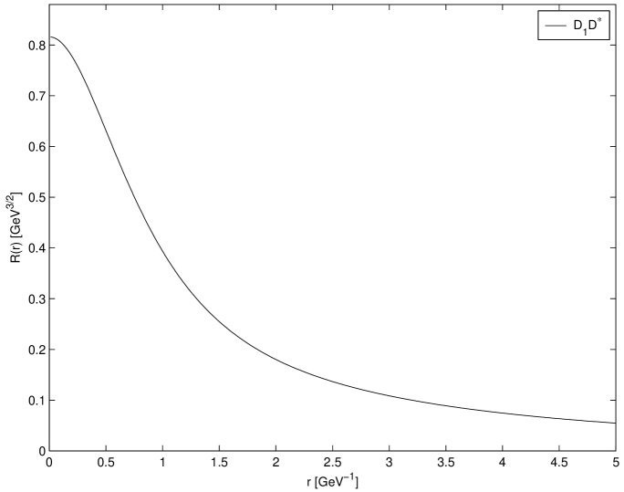
(a)	(b)

Figure 6: The radial wave function $R(r)$ for the molecular state with $J=0$ of the $D_{1}^{\prime}D^{*}$ and $D_{1}D^{*}$ system respectively. The corresponding parameters are [$g\cdot g^{\prime}$ = 0.1, $h$ = 0.84, $\Lambda$=1.5 GeV] and [$g\cdot g"$ = 0.2, $h^{\prime}$ = 0.55 GeV^-1, $\Lambda$=2.9 GeV] respectively.

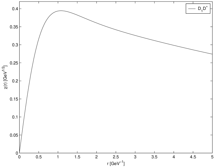
(a)	(b)	(c)

Figure 7: The function $\chi(r)=rR(r)$ for the J=0 molecular state of the $D_{1}^{\prime}D^{*}$ and $D_{1}D^{*}$ system. (c) shows the short range behavior for the $D_{1}D^{*}$ case. The corresponding parameters for the two systems are [$g\cdot g^{\prime}$ = 0.1, $h$ = 0.84, $\Lambda$=1.5 GeV] and [$g\cdot g^{\prime\prime}$ = 0.2, $h^{\prime}$ = 0.55 GeV^-1, $\Lambda$=2.9 GeV] respectively.

$D_{1}^{\prime}-D^{*}$ system
				$J=0$			$J=1$			$J=2$
$g\cdot g^{\prime}$	$h$	$g_{\sigma}\cdot g_{\sigma}^{\prime}$	$h_{\sigma}$	$E(\Lambda)$	$r_{rms}$	$r_{max}$	$E(\Lambda)$	$r_{rms}$	$r_{max}$	$E(\Lambda)$	$r_{rms}$	$r_{max}$
0.1	0.56	-	-	-2.8(0.7)	2.5	1.5	-2.9(0.7)	2.4	1.5	-3.1(0.7)	2.4	1.4
			0.4	-2.8(0.7)	2.5	1.5	-2.9(0.7)	2.4	1.5	-3.1(0.7)	2.4	1.4
		0.58	0.8	-2.8(0.7)	2.4	1.5	-2.9(0.7)	2.4	1.5	-3.1(0.7)	2.4	1.4
0.1	0.56		0.4	-2.8(0.7)	2.5	1.5	-2.9(0.7)	2.4	1.5	-3.1(0.7)	2.4	1.5
		-0.58	0.8	-2.8(0.7)	2.5	1.5	-2.9(0.7)	2.4	1.5	-3.1(0.7)	2.4	1.4
0.1	0.84	-	-	-23.9(0.7)/-5.5(1.5)	1.5/2.1	1.3/1.5	-24.1(0.7)/-5.6(1.5)	1.5/2.1	1.3/1.5	-24.5(0.7)/-5.8(1.5)	1.5/2.1	1.2/1.5
			0.4	-23.9(0.7)/-5.4(1.5)	1.5/2.1	1.3/1.5	-24.1(0.7)/-5.5(1.5)	1.5/2.1	1.3/1.5	-24.5(0.7)/-5.6(1.5)	1.5/2.1	1.2/1.5
		0.58	0.8	-24.1(0.7)/-5.5(1.5)	1.5/2.0	1.3/1.5	-24.1(0.7)/-5.5(1.5)	1.5/2.1	1.3/1.5	-24.5(0.7)/-5.7(1.5)	1.5/2.1	1.2/1.5
0.1	0.84		0.4	-23.9(0.7)/-5.6(1.5)	1.5/2.1	1.3/1.5	-24.1(0.7)/-5.7(1.5)	1.5/2.1	1.3/1.5	-24.5(0.7)/-5.9(1.5)	1.5/2.0	1.2/1.5
		-0.58	0.8	-23.9(0.7)/-5.9(1.5)	1.5/2.0	1.3/1.5	-24.1(0.7)/-5.8(1.5)	1.5/2.0	1.3/1.5	-24.5(0.7)/-5.9(1.5)	1.5/2.0	1.2/1.5
0.5	0.56	-	-	-2.0(0.7)	2.8	1.5	-2.4(0.7)	2.6	1.5	-3.6(0.7)	2.2	1.4
			0.4	-2.0(0.7)	2.8	1.5	-2.5(0.7)	2.6	1.5	-3.6(0.7)	2.2	1.4
		0.58	0.8	-2.0(0.7)	2.8	1.5	-2.5(0.7)	2.6	1.5	-3.5(0.7)	2.2	1.4
0.5	0.56		0.4	-2.0(0.7)	2.8	1.5	-2.5(0.7)	2.6	1.5	-3.6(0.7)	2.2	1.4
		-0.58	0.8	-2.0(0.7)	2.8	1.5	-2.5(0.7)	2.6	1.5	-3.6(0.7)	2.2	1.4
0.5	0.84	-	-	-22.3(0.7)/-5.0(1.5)	1.5/2.2	1.3/1.6	-23.3(0.7)/-5.3(1.5)	1.5/2.1	1.3/1.5	-25.3(0.7)/-6.2(1.5)	1.4/2.0	1.2/1.5
			0.4	-22.3(0.7)/-4.8(1.5)	1.5/2.2	1.3/1.6	-23.3(0.7)/-5.2(1.5)	1.5/2.1	1.3/1.5	-25.3(0.7)/-6.0(1.5)	1.4/2.0	1.2/1.5
		0.58	0.8	-22.3(0.7)/-4.7(1.5)	1.5/2.2	1.3/1.6	-23.3(0.7)/-5.1(1.5)	1.5/2.1	1.3/1.5	-25.3(0.7)/-6.0(1.5)	1.4/2.0	1.2/1.5
0.5	0.84		0.4	-22.3(0.7)/-5.1(1.5)	1.5/2.2	1.3/1.6	-23.3(0.7)/-5.4(1.5)	1.5/2.1	1.3/1.5	-25.3(0.7)/-6.3(1.5)	1.4/2.0	1.2/1.5
		-0.58	0.8	-22.4(0.7)/-5.0(1.5)	1.5/2.1	1.3/1.5	-23.3(0.7)/-5.4(1.5)	1.5/2.1	1.3/1.5	-25.3(0.7)/-6.3(1.5)	1.4/2.0	1.2/1.5
-0.1	0.56	-	-	-3.2(0.7)	2.3	1.4	-3.1(0.7)	2.3	1.4	-2.9(0.7)	2.4	1.4
			0.4	-3.2(0.7)	2.3	1.4	-3.1(0.7)	2.4	1.4	-2.9(0.7)	2.4	1.5
		0.58	0.8	-3.2(0.7)	2.3	1.4	-3.1(0.7)	2.4	1.4	-2.9(0.7)	2.4	1.5
-0.1	0.56		0.4	-3.2(0.7)	2.3	1.4	-3.1(0.7)	2.4	1.4	-2.9(0.7)	2.4	1.5
		-0.58	0.8	-3.2(0.7)	2.3	1.4	-3.1(0.7)	2.4	1.4	-2.9(0.7)	2.4	1.5
-0.1	0.84	-	-	-24.7(0.7)/-5.9(1.5)	1.4/2.0	1.2/1.5	-24.5(0.7)/-5.8(1.5)	1.5/2.0	1.2/1.5	-24.1(0.7)/-5.6(1.5)	1.5/2.1	1.3/1.5
			0.4	-24.7(0.7)/-5.7(1.5)	1.4/2.0	1.2/1.5	-24.5(0.7)/-5.6(1.5)	1.5/2.1	1.2/1.5	-24.1(0.7)/-5.5(1.5)	1.5/2.1	1.3/1.5
		0.58	0.8	-24.7(0.7)/-6.5(1.5)	1.4/1.9	1.2/1.5	-24.5(0.7)/-6.0(1.5)	1.5/2.0	1.2/1.5	-24.1(0.7)/-5.8(1.5)	1.5/2.1	1.3/1.5
-0.1	0.84		0.4	-24.7(0.7)/-6.0(1.5)	1.4/2.0	1.2/1.5	-24.5(0.7)/-5.9(1.5)	1.5/2.0	1.2/1.5	-24.1(0.7)/-5.7(1.5)	1.5/2.1	1.3/1.5
		-0.58	0.8	-24.7(0.7)/-6.5(1.5)	1.4/1.9	1.2/1.5	-24.5(0.7)/-6.0(1.5)	1.5/2.0	1.2/1.5	-24.1(0.7)/-5.8(1.5)	1.5/2.1	1.3/1.5
-0.5	0.56	-	-	-4.2(0.7)	2.1	1.4	-3.6(0.7)	2.2	1.4	-2.4(0.7)	2.6	1.5
			0.4	-4.2(0.7)	2.1	1.4	-3.6(0.7)	2.2	1.4	-2.4(0.7)	2.6	1.5
		0.58	0.8	-4.2(0.7)/-1.1(1.5)	2.1/3.3	1.4/1.4	-3.6(0.7)	2.2	1.4	-2.4(0.7)	2.6	1.5
-0.5	0.56		0.4	-4.2(0.7)/-0.1(1.5)	2.1/10.6	1.4/1.7	-3.6(0.7)	2.2	1.4	-2.4(0.7)	2.6	1.5
		-0.58	0.8	-4.2(0.7)/-1.6(1.5)	2.1/2.8	1.4/1.4	-3.6(0.7)	2.2	1.4	-2.4(0.7)	2.6	1.5
-0.5	0.84	-	-	-26.4(0.7)/-6.8(1.5)	1.4/2.0	1.2/1.5	-25.3(0.7)/-6.2(1.5)	1.4/2.0	1.2/1.5	-23.3(0.7)/-7.6(1.5)	1.5/2.1	1.3/1.5
			0.4	-26.4(0.7)/-6.8(1.5)	1.4/1.9	1.2/1.5	-25.3(0.7)/-6.0(1.5)	1.4/2.0	1.2/1.5	-23.3(0.7)/-5.2(1.5)	1.5/2.1	1.3/1.5
		0.58	0.8	-26.4(0.7)/-8.0(1.5)	1.4/1.8	1.2/1.4	-25.3(0.7)/-6.2(1.5)	1.4/2.0	1.2/1.5	-23.3(0.7)/-5.3(1.5)	1.5/2.1	1.3/1.5
-0.5	0.84		0.4	-26.4(0.7)/-7.2(1.5)	1.4/1.9	1.2/1.5	-25.3(0.7)/-6.4(1.5)	1.4/2.0	1.2/1.5	-23.3(0.7)/-5.5(1.5)	1.5/2.1	1.3/1.5
		-0.58	0.8	-26.4(0.7)/-8.6(1.5)	1.4/1.8	1.2/1.4	-25.3(0.7)/-6.6(1.5)	1.4/1.9	1.2/1.5	-23.3(0.7)/-5.6(1.5)	1.5/2.1	1.3/1.5

Table 3: The numerical results of $D_{1}^{\prime}-D^{*}$ system with $J^{P}=0^{-},1^{-},2^{-}$. Here the bing energy $E$, cutoff $\Lambda$, the root-mean-square radius $r_{rms}$ and $r_{max}$ of the $D_{1}^{\prime}-D^{*}$ system are in unit of MeV, GeV, fm and fm respectively. $E(\Lambda)$ denotes the binding energy with the corresponding cutoff.

V.2 S-wave $D_{1}-D^{*}$ system

In Table 4, we present the numerical results for the case of S-wave $D_{1}-D^{*}$ system. Unfortunately one fails to find solutions with negative binding energy for $J=1,2$ using the parameters in that table, which indicates that there probably does not exist the S-wave $D_{1}-D^{*}$ molecule with $J^{P}=1^{-},2^{-}$ through the pion and sigma exchange interactions. However the S-wave $D_{1}-D^{*}$ molecular state with $J^{P}=0^{-}$ probably exists. Thus we only present the results for the $D_{1}-D^{*}$ system with $J=0$.

When taking cutoff $\Lambda=2.9$ GeV, one gets $E=-1.3$ MeV with parameters $[g\cdot g^{\prime\prime},h^{\prime},g_{\sigma}\cdot g_{\sigma}^{\prime\prime},h_{\sigma}^{\prime}$]=[0.2,0.55 GeV^-1,0.58,0.2]. Varying parameters $g\cdot g^{\prime\prime}$, $g_{\sigma}\cdot g_{\sigma}^{\prime\prime}$, $h_{\sigma}^{\prime}$ in the reasonable range results in large change for the binding energy with fixed $\Lambda=2.9$ GeV, which indicates that the solutions are sensitive to coupling constants. Meanwhile one finds that one sigma exchange interaction induces significant effects. There exist solutions with the binding energies around $-10\sim 0$ MeV with appropriate coupling constants and cutoff, which are also shown in Table 4. We present the radial wave function $R(r)$ and function $\chi(r)=rR(r)$ for the $D_{1}-D^{*}$ system with $J=0$ in Fig. 6 (b) and Fig. 7 (b), (c) respectively.

One finds that big $g\cdot g^{\prime\prime}$, small $g_{\sigma}\cdot g_{\sigma}^{\prime\prime}$ and big $h_{\sigma}^{\prime}$ are beneficial to large binding energy. The results indicate that the larger the cutoff $\Lambda$ is, the deeper the binding.

$D_{1}-D^{*}$ system
				$J=0$
$g\cdot g^{\prime\prime}$	$h^{\prime}$	$g_{\sigma}\cdot g_{\sigma}^{\prime\prime}$	$h_{\sigma}^{\prime}$	E($\Lambda$)	$r_{rms}$(fm)	$r_{max}$(fm)
		0.0	0.0	-2.8(2.9)	1.8	0.2
			0.2	-1.3(2.9)	2.6	0.2
		0.58	1.0	-133.2(2.9)	0.3	0.2
0.2	0.55		0.2	-9.8(2.9)	1.0	0.2
		-0.58	1.0	-155.5(2.9)	0.3	0.2
		0.0	0.0	-196.4(2.9)	0.3	0.2
			0.2	-193.3(2.9)	0.3	0.2
		0.58	1.0	-4.6(2.0)/-427.0(2.9)	1.5/0.2	0.4/0.1
0.6	0.55		0.2	-217.0(2.9)	0.3	0.2
		-0.58	1.0	-9.1(2.0)/-453.6(2.9)	1.1/0.2	0.4/0.1
		0.0	0.0	$\times$	$\times$	$\times$
			0.2	$\times$	$\times$	$\times$
		0.58	1.0	$\times$	$\times$	$\times$
-0.2	0.55		0.2	$\times$	$\times$	$\times$
		-0.58	1.0	$\times$	$\times$	$\times$
		0.0	0.0	$\times$	$\times$	$\times$
			0.2	$\times$	$\times$	$\times$
		0.58	1.0	$\times$	$\times$	$\times$
-0.6	0.55		0.2	$\times$	$\times$	$\times$
		-0.58	1.0	$\times$	$\times$	$\times$

Table 4: Numerical results for the $D_{1}-D^{*}$ system with several sets of parameters if we use $\Lambda=2.0$ GeV and $\Lambda=2.9$ GeV. The unit is MeV. Negative bound energies exist only for $J=0$. The cross $\times$ means no bound state exists. If we use a smaller cutoff $\Lambda=0.7$ GeV, there are no bound state solutions with the parameters in this table.

VI Bottom analog

The calculation can be easily extended to study the bottom analog of $Z^{+}(4430)$. For such a system, its flavor wavefunction is

$$|Z_{B}^{+}\rangle=\frac{1}{\sqrt{2}}\Big{[}|B_{1}^{{}^{\prime}+}\bar{B}^{*0}\rangle+|B^{*+}\bar{B}_{1}^{{}^{\prime}0}\rangle\Big{]}$$ (29)

or

$$|Z_{B}^{+}\rangle=\frac{1}{\sqrt{2}}\Big{[}|B_{1}^{+}\bar{B}^{*0}\rangle+|B^{*+}\bar{B}_{1}^{0}\rangle\Big{]}.$$ (30)

$B_{1}^{\prime}-B^{*}$ system
		$J=0$			$J=1$			$J=2$
$g\cdot g^{\prime}$	$h$	E(MeV)	$r_{rms}$(fm)	$r_{max}$(fm)	E(MeV)	$r_{rms}$(fm)	$r_{max}$(fm)	E(MeV)	$r_{rms}$(fm)	$r_{max}$(fm)
0.1	0.56	-2.6	2.0	1.6	-2.6	2.0	1.6	-2.8	2.0	1.6
0.1	0.84	-14.6	1.6	1.5	-14.7	1.5	1.5	-14.7	1.6	1.5
0.5	0.56	-2.3	2.1	1.6	-2.5	2.1	1.6	-3.2	1.9	1.5
0.5	0.84	-14.5	1.7	1.5	-14.6	1.7	1.5	-14.9	1.6	1.5
-0.1	0.56	-2.9	2.0	1.6	-2.8	2.0	1.6	-2.6	2.0	1.6
-0.1	0.84	-14.8	1.6	1.5	-14.7	1.6	1.5	-14.7	1.6	1.5
-0.5	0.56	-4.4	1.7	1.4	-3.2	1.9	1.5	-2.5	2.1	1.6
-0.5	0.84	-15.3	1.6	1.5	-14.9	1.6	1.5	-14.6	1.7	1.5

Table 5: Numerical results for the $B_{1}^{\prime}-B^{*}$ system with several sets of parameters and $\Lambda=1.5$ GeV.

$B_{1}-B^{*}$ system
				$J=0$
$g\cdot g^{\prime\prime}$	$h^{\prime}$	$g_{\sigma}\cdot g_{\sigma}^{\prime\prime}$	$h_{\sigma}^{\prime}$	E($\Lambda$)	$r_{rms}$(fm)	$r_{max}$(fm)
		0.0	0.0	-1.0(1.9)	1.9	0.4
			0.2	-0.2(1.9)	4.3	0.4
		0.58	1.0	-26.9(1.9)	0.5	0.3
0.2	0.55		0.2	-3.6(1.9)	1.1	0.3
		-0.58	1.0	-35.3(1.9)	0.5	0.2
		0.0	0.0	-0.2(1.2)/-60.7(1.9)	4.4/0.4	0.7/0.2
			0.2	-0.1(1.2)/-58.1(1.9)	7.5/0.4	0.7/0.2
		0.58	1.0	-1.3(1.2)/-111.1(1.9)	1.8/0.3	0.6/0.2
0.6	0.55		0.2	-0.4(1.2)/-67.4(1.9)	3.0/0.4	0.7/0.2
		-0.58	1.0	-2.1(1.2)/-121.4(1.9)	1.5/0.3	0.6/0.2
		0.0	0.0	$\times$	$\times$	$\times$
			0.2	$\times$	$\times$	$\times$
		0.58	1.0	$\times$	$\times$	$\times$
-0.2	0.55		0.2	$\times$	$\times$	$\times$
		-0.58	1.0	$\times$	$\times$	$\times$
		0.0	0.0	$\times$	$\times$	$\times$
			0.2	$\times$	$\times$	$\times$
		0.58	1.0	$\times$	$\times$	$\times$
-0.6	0.55		0.2	$\times$	$\times$	$\times$
		-0.58	1.0	$\times$	$\times$	$\times$

Table 6: Numerical results for the $B_{1}-B^{*}$ system with several sets of parameters if we use $\Lambda=1.2$ GeV and $\Lambda=1.9$ GeV. Here $E(\Lambda)$ denotes the binding energy with corresponding cutoff. The unit is MeV. Negative bound energies exist only for $J=0$.

The masses of the bottom mesons are $m_{B^{\ast}}=5325.0$ MeV, $m_{B_{1}}=5725.3$ MeV and $m_{B_{1}^{\prime}}=5732$ MeV PDG ; PDG-1 . Since $m_{B_{1}^{\prime}}-m_{B^{\ast}}$ or $m_{B_{1}}-m_{B^{\ast}}$ is greater than the pion mass and less than $\sigma$ mass, the forms of the potentials are exactly those given in Table 1 and 2. The difference between the charmed and bottom systems lies only in the meson masses. The relatively small kinematic term makes it easier to form molecular states in the bottom system.

From the results for the $D_{1}^{\prime}D^{\ast}$ system (Table 3), one sees that the $\sigma$ exchange gives negligible contributions to the binding energy of the system. The same conclusion holds for the $B_{1}^{\prime}B^{\ast}$ system. Thus we ignore effects from $\sigma$ exchange in the numerical evaluation. We choose eight sets of parameters to calculate: [$g\cdot g^{\prime}$, $h$]=[$\pm 0.1$, 0.56], [$\pm 0.5$, 0.56], [$\pm 0.1$, 0.84] and [$\pm 0.5$, 0.84]. The results are given in Table 5 where we use the cutoff $\Lambda=1.5$ GeV. With this cutoff, a bound state always exists with reasonable couplings.

For the system of $B_{1}B^{\ast}$, we use the same sets of parameters in Table 4 since the contribution from the $\sigma$ exchange may be large. We list the results in Table 6 where two values of $\Lambda$ 1.2 GeV and 1.9 GeV, are used. This case is similar to the case of the $D_{1}D^{\ast}$ case. The bound states with $J=0$ may exist with the positive $g\cdot g^{\prime\prime}$.

VII The cutoff dependence

Up to now, we have solved the radial Schroding equation with only a few values of the cutoff $\Lambda$. But the binding energies will change with the variation of this parameter. We briefly study the cutoff dependence of the binding energy.

Since a bound state is more easily formed in the bottom system, we first study the system $B_{1}^{\prime}B^{\ast}$ with $g\cdot g^{\prime}=-0.5$ and $h=0.84$ for $J=0$. By scanning results starting from $\Lambda=0.7$ GeV, we find the binding energy has a smallest value around $\Lambda=2.3$ GeV. One can always find negative eigenvalues with $g\cdot g^{\prime}=-0.5$ and $h=0.84$ for this case. The dependence of the binding energies on the cutoff is not monotonic. We also study results with other couplings and $J$. This conclusion is always correct for the $B_{1}^{\prime}B^{\ast}$ system. Some minimum binding energies with corresponding $\Lambda$ are presented in Table 7.

Systems	$g\cdot g^{\prime}$	$h$	$g_{\sigma}\cdot g_{\sigma}^{\prime}$	$h_{\sigma}$	$J=0$	$J=1$	$J=2$
$B_{1}^{\prime}{B}^{\ast}$	-0.5	0.84	0	0	-14.4(2.3)	-14.0(3.5)	-14.4(2.1)
	0.5	0.56	0	0	-2.3(1.4)	-2.4(1.8)	-2.8(2.4)
$D_{1}^{\prime}{D}^{\ast}$	-0.5	0.84	-0.58	0.8	-8.6(1.5)	-5.9(2.1)	-5.5(1.7)

Table 7: Minimum binding energies $E$ with the corresponding cutoff $\Lambda$ for some sets of coupling constants. The unit for $E(\Lambda)$ is MeV(GeV).

It is interesting to study whether similar behavior exists in the other systems. For the $D_{1}^{\prime}{D}^{\ast}$ system, the minimum binding energy exists only for some coupling constants. One example is presented in Table 7. For the solutions with $h=0.56$, the binding energy decreases if we increase $\Lambda$ until the $D_{1}^{\prime}{D}^{\ast}$ pair is no longer bound. Thus bound states exist only in a small range of $\Lambda$.

For the $D_{1}{D}^{\ast}$ and $B_{1}{B}^{\ast}$ systems, the solutions for bound states can be found only when $\Lambda$ is big enough. The binding energy becomes large with the increase of the cutoff.

In short summary, we have studied the cutoff dependence for the binding energies with some sets of coupling constants. Three types of behavior are found: (1) bound state solutions always exist whatever the $\Lambda$ is. In this case, the binding energy reaches the minimum value at a special $\Lambda$; (2) bound state solutions exist with small $\Lambda$ only. The binding energy becomes large when the cutoff becomes small; (3) bound state solutions exist when $\Lambda$ is big enough. In this case, the binding energy increases with the cutoff. Which case is realized for a system depends on the properties of the components and the values of the coupling constants. One should also keep in mind the cutoff is a typical hadronic scale related to the system.

VIII Conclusions

QCD allows the possible existence of the glueball, hybrids, multiquarks and molecular states etc. However, none of them has been established firmly. Recently Belle collaboration announced the observation of charged enhancement $Z^{+}(4430)$, whose unique properties make $Z^{+}(4430)$ hardly understood as a conventional meson. A natural explanation of $Z^{+}(4430)$ is the $D_{1}^{{}^{\prime}}D^{*}$ or $D_{1}D^{*}$ molecule state.

In this work, we re-examine the dynamics of $Z^{+}(4430)$ and improve the analysis in Ref. xiangliu in the following aspects: (1) we include the sigma meson exchange contribution besides the one pion exchange potential; (2) we introduce the form factor to take into account the structure effect of the interaction vertex; (3) we solve the schrödinger equation of the S-wave $D_{1}^{{}^{\prime}}D^{*}$ or $D_{1}D^{*}$ system with the help of Matlab package MATSLISE.

We find that the one pion exchange potential from the crossed diagram plays a dominant role for the S-wave $D_{1}^{\prime}D^{*}$ or $D_{1}D^{*}$ system. Our numerical results indicate that with the coupling constants determined in Section II there exists the S-wave $D_{1}^{\prime}D^{*}$ molecular state with $J^{P}=0^{-},1^{-},2^{-}$. The sigma meson exchange contribution to the binding energy is small. However one should carefully study whether the broad width of $D_{1}^{\prime}$ disfavors the formation of a molecular state in the future.

For the S-wave $D_{1}-D^{*}$ system, only a molecular state with $J^{P}=0^{-}$ may exist with appropriate parameters. The contribution from the sigma meson exchange is significant in this case. Replacing the charmed meson masses with bottom meson masses, we have also studied the bottom analogy $Z_{B}$ of the $Z(4430)$ system. As expected, the absolute value of the binding energy of $Z_{B}$ is larger than that of $Z(4430)$. Such a state may be searched for at Tevatron and LHC. Clearly future experimental measurement of the quantum numbers of $Z(4430)$ will help uncover its underlying structure.

References

• (1) Belle Collaboration, K. Abe et al., arXiv:0708.1790 [hep-ex].
• (2) X. Liu, Y.R. Liu, W.Z. Deng and S.L. Zhu, Phys. Rev. D 77, 034003 (2008).
• (3) J.L. Rosner, Phys. Rev. D 76, 114002 (2007).
• (4) C. Meng and K.T. Chao, arXiv:0708.4222 [hep-ph].
• (5) D.V. Bugg, arXiv:0709.1254 [hep-ph]; arXiv:0802.0934 [hep-ph].
• (6) K. Cheung, W.Y. Keung and T.C. Yuan, Phys. Rev. D 76, 117501 (2007).
• (7) L. Maiani, A.D. Polosa and V. Riquer, arXiv:0708.3997 [hep-ph].
• (8) S.S. Gershtein, A.K. Likhoded and G.P. Pronko, arXiv:0709.2058 [hep-ph].
• (9) C.F. Qiao, arXiv:0709.4066 [hep-ph].
• (10) S.H. Lee, A. Mihara, F.S. Navarra and M. Nielsen, arXiv:0710.1029 [hep-ph].
• (11) Y. Li, C.D. Lu and W. Wang, arXiv: 0711.0497 [hep-ph].
• (12) G.J. Ding, arXiv:0711.1485 [hep-ph].
• (13) E. Braaten and M. Lu, arXiv:0712.3885 [hep-ph].
• (14) X.H. Liu, Q. Zhao and F.E. Close, arXiv: 0802.2648 [hep-ph].
• (15) M. B. Voloshin, arXiv:0711.4556 [hep-ph].
• (16) A. D. Polosa, arXiv:0712.1691 [hep-ph].
• (17) S. Godfrey, S. L. Olsen, arXiv:0801.3867 [hep-ph].
• (18) Y.R. Liu, X. Liu, W.Z. Deng and S.L. Zhu, arXiv:0801.3540 [hep-ph].
• (19) A. F. Falk and M. Luke, Phys. Lett. B 292, 119 (1992).
• (20) R. Casalbuoni, A. Deandrea, N. Di Bartolomeo, F. Feruglio, R. Gatto and G. Nardulli, Phys. Rept. 281, 145 (1997).
• (21) W.A. Bardeen, E.J. Eichten and C.T. Hill, Phys. Rev. D 68, 054024 (2003).
• (22) V.M. Belyaev, V. M. Braun, A. Khodjamirian and R. Ruckl, Phys. Rev. D 51, 6177 (1995).
• (23) F. S. Navarra, Marina Nielsen and M.E. Bracco, Phys. Rev. D 65, 037502 (2002).
• (24) F. S. Navarra, M. Nielsen, M. E. Bracco, M. Chiapparini and C.L. Schat, Phys. Lett. B 489, 319 (2000).
• (25) Y. B. Dai and S. L. Zhu, Eur. Phys. J. C 6, 307 (1999).
• (26) CLEO collaboration, S. Ahmed et. al., Phys. Rev. Lett. 87, 251801 (2001); C. Isola, M. Ladisa, G. Nardulli and P. Santorelli, Phys. Rev. D 68, 114001 (2003).
• (27) N. A. TΓΆrnqvist, Z. Phys. C 61, 525 (1994).
• (28) M.P. Locher, Y. Lu, and B. S. Zou, Z. Phys. A 347, 281 (1994) ; X.Q. Li, D.V. Bugg, and B.S. Zou, Phys. Rev. D 55, 1421 (1997); X.G. He, X.Q. Li, X. Liu and X.Q. Zeng, Eur. Phys. J. C 51, 883-889 (2007), arXiv:hep-ph/0606015; X. Liu, X.Q. Zeng and X.Q. Li, Phys. Rev. D 74, 074003 (2006), arXiv: hep-ph/0606191.
• (29) W. M. Yao et al., Particle Data Group, J. Phys. G 33, 1 (2006).
• (30) V. LEDOUX, M.V. DAELE and G.V. BERGHE, Comp. Phys. Commun. 162, 151 (2004); V. LEDOUX, M.V. DAELE and G.V. BERGHE, ACM Transactions on Mathematical Software 31, 532-554 (2005); http://users.ugent.be/Β vledoux/MATSLISE/.
• (31) CDF Collaboration, β€œMass and width measurement of orbitally excited ($L=1$) $B^{**0}$ mesons”, CDF Note 8945, www-cdf.fnal.gov/physics/new/bottom/070726.blessed-bss/; CDF Collaboration, Andreas Gessler, the EPS talk given on HEP 2007 in Manchester, arXiv:0709.3148 [hep-ex].