Radiative and dilepton decays of the hadronic molecule $Z_{c}^{+}(3900)$

Abstract

The newly observed hidden-charm meson $Z_{c}^{+}(3900)$ with quantum numbers $J^{P}=1^{+}$ is considered as a hadronic molecule composed of $\bar{D}D^{\ast}$. We give detailed predictions for the decay modes $Z_{c}^{+}\to{J/\psi}\pi^{+}\gamma$ and $Z_{c}^{+}\to{J/\psi}\pi^{+}\ell^{+}\ell^{-}$ $(\ell=e,\mu)$ in a phenomenological Lagrangian approach.

I Introduction

Recently the three experimental collaborations BESIII Ablikim:2013mio , Belle Liu:2013dau and CLEO-c Xiao:2013iha reported on the observation of a new charged resonance $Z_{c}(3900)$ detected via the decay channel $J/\psi\pi^{\pm}$. This observation of a charged, hidden charm state embedded in the charmonium spectrum presents clear evidence for an exotic meson resonance. Interpretations of this unusual state were immediately presented, dominantly focusing on either a compact tetraquark configuration Faccini:2013lda ; Dias:2013xfa ; Braaten:2013boa or a molecular state Wang:2013cya ; Cui:2013yva ; Zhang:2013aoa ; Ke:2013gia ; Dong:2013iqa .

One of the tools in identifying the underlying structure rests on the study of the decay patterns of the $Z_{c}$ in addition to the discovery decay mode $J/\psi\pi^{\pm}$. For example, predictions for the strong two-body transitions $Z_{c}^{+}\to H+\pi^{+}$ with $H=\Psi(nS)$, $h_{c}(mP)$ were already worked out in the context of a hadronic molecule interpretation Dong:2013iqa (see also extension on bottom sector $Z_{b}$ Dong:2012hc ). In the present work we extend to the radiative and dilepton decays of the hadronic molecule $Z_{c}^{+}(3900)$ proceeding as $Z_{c}^{+}\to{J/\psi}\pi^{+}\gamma$ and $Z_{c}^{+}\to{J/\psi}\pi^{+}\ell^{+}\ell^{-}$ $(\ell=e,\mu)$. Radiative and dilepton decays can shed light on the composite structure of the $Z_{c}^{+}(3900)$: decay patterns and decay widths will depend on the structure assumption such as a hadronic molecule, a tetraquark configuration or even a mixed state of these components. Although radiative decays are suppressed due to the strength of the interaction particular final states such as $J/\psi\pi^{+}\gamma$ are relatively easy to identify experimentally. The analysis is based on a phenomenological Lagrangian approach Faessler:2007gv ; Dong:2012hc ; Dong:2013kta together with the compositeness condition Weinberg:1962hj ; Efimov:1993ei ; Branz:2009cd , which is a powerful tool to formulate hadrons as bound states of their constituents using methods of quantum field theory.

When treating the $Z_{c}^{+}$ as a hadronic molecule we assume that this state together with the negative $Z_{c}(3900)^{-}$ and the neutral $Z_{c}(3900)^{0}$ partners form an isospin triplet with spin and parity quantum numbers $J^{P}=1^{+}$ [as for example briefly discussed in Ref. Dong:2013kta ]. Therefore the charged hidden-charm meson resonance $Z_{c}^{+}$ is set up as a superposition of the molecular configurations $\bar{D}D^{*}$ as

$$|Z_{c}^{+}\rangle = \frac{1}{\sqrt{2}}\Big{|}D^{*+}\bar{D}^{0}+\bar{D}^{*0}D^{+}\Big{\rangle}\,.$$ (1)

Note that analogous states in the bottom sector ($Z_{b}^{+}$ and $Z_{b}^{{}^{\prime}+}$) have also been considered previously Ref. Dong:2012hc .

To evaluate the radiative and dilepton decays of the molecular state $Z_{c}^{+}$ we proceed in the present paper as follows. In Sec. II we briefly review the basic ideas of our approach. We set up the new resonance $Z_{c}^{+}$ as a $\bar{D}D^{\ast}$ molecular state and specify the relevant interaction Lagrangians for the description of the three- and four-body decays $Z_{c}^{+}\to{J/\psi}\pi^{+}\gamma$ and $Z_{c}^{+}\to{J/\psi}\pi^{+}\ell^{+}\ell^{-}$ $(\ell=e,\mu)$. In Sec. III we introduce and discuss the kinematics of the many-body transitions. In Sec. IV we present numerical results and the discussion.

II Framework

Our approach to the molecular $Z_{c}^{+}$ state is based on an interaction Lagrangian describing its coupling to the constituents as

$${\cal L}^{0}_{Z_{c}DD^{\ast}}(x) = Z_{c}^{+\mu}(x)\bar{J}_{Z_{c}}^{\mu}(x)+Z_{c}^{-\mu}(x)J_{Z_{c}}^{\mu}(x)\,,$$

$$J_{Z_{c}}^{\mu}(x) = \frac{g_{{}_{Z_{c}}}}{\sqrt{2}}\,M_{Z_{c}}\,\int d^{4}y\,\Phi_{Z_{c}}(y^{2})$$ (2)

$$\times \left(D^{+}(x_{+})\bar{D}^{*0}_{\mu}(x_{-})+D^{*+}_{\mu}(x_{+})\bar{D^{0}}(x_{-})\right)$$

where $x_{+}\equiv x+w_{1}\,y$, $x_{-}\equiv x-w_{2}\,y$. Here $x$ is the center-of-mass coordinate, $y$ is the relative (Jacobi) coordinate of the constituents and $w_{1}=m_{D}/(m_{D}+m_{D^{\ast}})$ and $w_{2}=m_{D^{\ast}}/(m_{D}+m_{D^{\ast}})$ are the fractions of the masses of the constituents. The dimensionless constant $g_{{}_{Z_{c}}}$ describes the coupling strength of the $Z_{c}^{+}$ to the molecular $\bar{D}D^{*}$ components. $\Phi_{Z_{c}}(y^{2})$ is a correlation function which describes the distribution of the constituent mesons in the bound state. A basic requirement for the choice of an explicit form of the correlation function $\Phi_{Z_{c}}(y^{2})$ is that its Fourier transform vanishes sufficiently fast in the ultraviolet region of Euclidean space to render the Feynman diagrams ultraviolet finite. We adopt a Gaussian form for the correlation function. The Fourier transform of this vertex function is given by $\tilde{\Phi}_{Z_{c}}(p_{E}^{2}/\Lambda^{2})\equiv\exp(-p_{E}^{2}/\Lambda^{2})$, where $p_{E}$ is the Euclidean Jacobi momentum. $\Lambda$ is a size parameter characterizing the distribution of the two constituent mesons in the $Z_{c}^{+}$ system. For a molecular system where the binding energy is negligible in comparison with the constituent masses this size parameter is expected to be smaller than 1 GeV. From our previous analyses of the strong two-body decays of the $X,Y,Z$ meson resonances and of the $\Lambda_{c}(2940)$ and $\Sigma_{c}(2880)$ baryon states we deduced a value of maximally $\Lambda\sim 1$ GeV Dong:2009tg . For a very loosely bound system like the $X(3872)$ a size parameter of $\Lambda\sim 0.5$ GeV Dong:2009uf is more suitable. Here we choose values for $\Lambda$ in the range of $0.5-0.75$ GeV which reflect a weakly bound heavy meson system. Once $\Lambda$ is fixed the coupling constant $g_{{}_{Z_{c}}}$ is then determined by the compositeness condition Dong:2013iqa ; Faessler:2007gv ; Branz:2009cd . It implies that the renormalization constant of the hadron wave function is set equal to zero with:

$$Z_{Z_{c}}=1-\Sigma_{Z_{c}}^{\prime}(M_{Z_{c}}^{2})=0\,.$$ (3)

$\Sigma_{Z_{c}}^{\prime}$ is the derivative of the transverse part of the mass operator $\Sigma_{Z_{c}}^{\mu\nu}$ of the molecular states [see Fig. 1], which is defined as

$$\Sigma_{Z_{c}}^{\mu\nu}(p)=\biggl{(}g^{\mu\nu}-\frac{p^{\mu}p^{\nu}}{p^{2}}\biggr{)}\,\Sigma_{Z_{c}}(p)+\frac{p^{\mu}p^{\nu}}{p^{2}}\Sigma_{Z_{c}}^{L}(p)$$ (4)

We would like to stress again, that the size effects of the constituent $D$ mesons in the $Z_{c}^{+}(3900)$ are taken into account by the dimensional parameter $\Lambda$ and the coupling constant $g_{Z_{c}}$. These parameters are constrained by the compositeness condition (4) — the key condition for a study of bound states in quantum field theory. It is equivalent to the normalization of the wave function in Bethe-Salpeter approaches and to the Ward identity, relating hadronic electromagnetic vertex functions to the derivative of their mass operators on the mass-shell (see detailed discussion in Refs. Weinberg:1962hj ; Efimov:1993ei ; Branz:2009cd ).

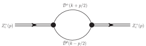
Figure 1: Mass operator for the $Z_{c}$.

An analytical expression for the coupling $g_{{}_{Z_{c}}}$ is given in Appendix A. In the calculation the mass of the $Z_{c}$ is expressed in terms of the constituent masses and the binding energy $\epsilon$ (a variable quantity in our calculations): $m_{Z_{c}}=m_{D}+m_{D^{\ast}}-\epsilon$  where $\epsilon$ is the binding energy. In order to calculate the three- and four-body decays $Z_{c}^{+}\to{J/\psi}\pi^{+}\gamma$ and $Z_{c}^{+}\to{J/\psi}\pi^{+}\ell^{+}\ell^{-}$ $(\ell=e,\mu)$ we need to specify additional phenomenological Lagrangians. Their interaction vertices occur in meson-loop diagrams which generate the decay modes. For this purpose the lowest-order Lagrangian $\cal L$ is given by

$${\cal L}(x) = {\cal L}_{Z_{c}}(x)+{\cal L}_{Z_{c}DD^{\ast}}(x)+{\cal L}_{DD^{\ast}{J/\psi}\pi}(x)$$ (5)

$$+ {\cal L}_{D}(x)+{\cal L}_{D^{\ast}}(x)+{\cal L}_{\pi}(x)+{\cal L}_{{J/\psi}}(x)$$

where

$${\cal L}_{V}(x) = -\frac{1}{4}G_{\mu\nu}(x)G^{\mu\nu}(x)-\frac{1}{2}M_{V}^{2}V_{\mu}(x)V^{\mu}(x)\,,$$

$${\cal L}_{S}(x) = \frac{1}{2}(D^{\mu}S(x))^{2}-\frac{1}{2}m_{S}^{2}S^{2}(x)$$ (6)

are the free Lagrangians of the spin-1 mesons $V=Z_{c},D^{\ast},{J/\psi}$ and spin-0 mesons $S=\pi,D$, respectively; $G^{\mu\nu}=\nabla^{\mu}V^{\nu}-\nabla^{\nu}V^{\mu}$ is the stress tensor of vector/axial mesons, $\nabla^{\mu}=\partial^{\mu}-ieA^{\mu}$ is the covariant derivative including the electromagnetic field in case of charged states and $e$ is the corresponding electric charge of hadron $H$. The Lagrangian ${\cal L}_{Z_{c}DD^{\ast}}(x)$ is the gauge-invariant extension of the strong $Z_{c}^{+}DD^{\ast}$ interaction Lagrangian (II). It includes photons by gauging with the path integral $I(x,y)=\int_{x}^{y}A_{\mu}dw^{\mu}$ resulting in

$${\cal L}_{Z_{c}DD^{\ast}}(x) = \frac{g_{{}_{Z_{c}}}}{\sqrt{2}}\,M_{Z_{c}}\,Z_{c}^{-\mu}(x)\!\int\!d^{4}y\Phi_{Z_{c}}(y^{2})e^{-ieI(x_{+},x)}$$ (7)

$$\times \left(D^{+}(x_{+})\bar{D}^{*0}_{\mu}(x_{-})+D^{*+}_{\mu}(x_{+})\bar{D^{0}}(x_{-})\right)$$

$$+ {\rm H.c.}$$

This Lagrangian is manifestly gauge-invariant. As discussed in detail in Refs. Anikin:1995cf -Faessler:2006ky , the presence of the vertex form factor in the interaction Lagrangian [like the strong-interaction Lagrangian describing the coupling of $Z_{c}$ to its constituents (Eq. II)] requires special care in establishing gauge invariance. One of the possibilities is provided by a modification of the charged fields which are multiplied by an exponential containing the electromagnetic field and the electrical charge $e$. This procedure was first suggested in Ref. Mandelstam:1962mi and applied in Refs. Terning:1991yt ; Faessler:2007gv ; Faessler:2007us ; Faessler:2007cu ; Faessler:2003yf . In doing so the fields of the charged ${\cal D}=D,D^{\ast}$ mesons are modified as

$${\cal D}^{+}(x_{+})\ \rightarrow\ e^{-ieI(x_{+},x,P)}{\cal D}^{+}(x_{+})\,,$$ (8)

which leads to the electromagnetic gauge-invariant Lagrangian (7). The interacting terms up to first order in $A^{\mu}$ are obtained by expanding ${\cal L}_{Z_{c}DD^{\ast}}(x)$ in terms of $I(x_{+},x)$. Diagrammatically the first order term gives rise to a nonlocal vertex with an additional photon line attached [see Fig. 4].

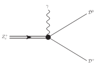
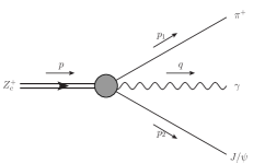
Figure 2: Photon attached to the nonlocal vertex.

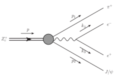
Figure 3: Notation for the kinematics of the process
$Z_{c}^{+}\to{J/\psi}\pi^{+}\gamma$.

Figure 4: Notation for the kinematics of the process
$Z_{c}^{+}\to{J/\psi}\pi^{+}\gamma[\to e^{+}e^{-}]$.

In the calculation of the three- and four-body decays $Z_{c}^{+}\to{J/\psi}\pi^{+}\gamma$ and $Z_{c}^{+}\to{J/\psi}\pi^{+}\ell^{+}\ell^{-}$ $(\ell=e,\mu)$ we also need the four-particle $DD^{\ast}{J/\psi}\pi$ vertex generated by a phenomenological Lagrangian proposed in Ref. Dong:2013iqa

$${\cal L}_{DD^{\ast}{J/\psi}\pi}(x) = -g_{DD^{\ast}{J/\psi}\pi}J^{\mu\nu}(x)\,\bar{D}^{\ast}_{\nu}(x)\,\nabla_{\mu}\hat{\pi}(x)\,D(x)$$ (9)

$$+ {\rm H.c.}$$

where $\nabla_{\mu}$ is the covariant derivative. The coupling constant $g_{DD^{\ast}{J/\psi}\pi}$ is given by

$$g_{DD^{\ast}{J/\psi}\pi}=\frac{\sqrt{6}}{2\sqrt{2}}\frac{g_{JDD}g_{D^{\ast}D\pi}}{(m_{Z_{c}}^{2}-m_{{J/\psi}}^{2})(1+\frac{m_{{J/\psi}}^{2}}{2m_{Z_{c}}^{2}})}\,,$$ (10)

as defined in Ref. Dong:2013iqa . The numerical value for $g_{JDD}g_{D^{\ast}D\pi}/2\sqrt{2}$ was evaluated in Ref. Dong:2013iqa and is expressed through $g_{JDD}g_{D^{\ast}D\pi}/2\sqrt{2}=47.08$. $\hat{\pi}$ is the pion matrix

$$\hat{\pi}=\vec{\pi}\cdot\vec{\tau}=\begin{pmatrix}\pi^{0}&\pi^{+}\sqrt{2}\\ \pi^{-}\sqrt{2}&-\pi^{0}\\ \end{pmatrix}$$ (11)

and $J^{\mu\nu}=\partial^{\mu}J^{\nu}-\partial^{\nu}J^{\mu}$ is the stress tensor of the ${J/\psi}$ state. $D=(D^{+},D^{0})$, $D^{\ast}=(D^{*+},D^{*0})$ are the doublets of pseudoscalar and vector charmed $D$ mesons, respectively. To simplify the calculations we neglect the transverse part of the vector propagators and of all vertex factors where the vector fields are involved. This is justified by the fact that the transverse parts only give a minor contribution to the transition amplitude. For a better and compact overview the external momenta of the three- and four-body decays are summarized in Figs. 3 and 4, respectively. To summarize we also indicate the respective Feynman rules in Appendix B.

The graphs governing the three-body decay $Z_{c}^{+}\to{J/\psi}\pi^{+}\gamma$ are shown in Figs. 6 and 6.

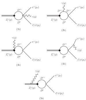
Figure 5: $\bar{D^{*0}}D^{+}$ meson loop diagrams contributing to the three-body decay $Z_{c}^{+}\to{J/\psi}\pi^{+}\gamma$.

Figure 6: $\bar{D^{0}}D^{*+}$ meson loop diagrams contributing to the three-body decay $Z_{c}^{+}\to{J/\psi}\pi^{+}\gamma$.

The diagrams are evaluated using the Schwinger representation for the propagators:

$$\frac{1}{m^{2}-k^{2}}=\int_{0}^{\infty}d\alpha\,e^{-\alpha(m^{2}-k^{2})}\,.$$ (12)

The resulting matrix element for the three-body decay $Z_{c}^{+}\to{J/\psi}\pi^{+}\gamma$ is gauge invariant as shown in Appendix C. It can be decomposed into the following Lorentz structures:

$${\cal T}^{\alpha\beta\rho} = \sum\limits_{i=1}^{5}{\cal T}^{\alpha\beta\rho}_{i}=\left(g^{\alpha\beta}p_{2}^{\rho}-p_{2}^{\alpha}g^{\beta\rho}\right)\,F_{1}$$ (13)

$$+ \left(p_{2}\cdot p_{1}g^{\alpha\beta}-p_{2}^{\alpha}p_{1}^{\beta}\right)p^{\rho}\,F_{235}$$

$$+ \left((p-p_{2})\cdot p_{2}g^{\alpha\beta}-p_{2}^{\alpha}p^{\beta}\right)p_{1}^{\rho}\,F_{4}$$

where with $F_{1}$, $F_{235}=F_{2}+F_{3}+F_{5}$ and $F_{4}$ we denote structure integrals collected in Appendix D. Since the diagrams $(2,3,5)$ in Fig. 6 and Fig. 6 have the same Lorentz structure they can be summed up together.

The matrix element ${\cal M}^{\alpha\beta}$ for the four-body decay $Z_{c}^{+}\to{J/\psi}\pi^{+}\ell^{+}\ell^{-}$ can be simply deduced from the matrix element for the three-body decay. We assume that only the photon contributes through conversion to the dilepton final state. Hence the matrix element for the four-body decay factorizes into a three-body part ${\cal T}$ of the $Z_{c}^{+}\to{J/\psi}\pi^{+}\gamma$ transition and a leptonic part $\ell$ corresponding to the dilepton production $\gamma\to\ell^{+}\ell^{-}$:

$${\cal M}^{\alpha\beta}=-\,\frac{e^{2}}{t}\ {\cal T}^{\alpha\beta\rho}\ \ell_{\rho}$$ (14)

where $t=(k_{3}+k_{4})^{2}$, $\ell^{\rho}=\bar{u}(k_{3})\,\gamma^{\rho}\,v(k_{4})$ is the leptonic current and $\bar{u}(k_{3})$, $v(k_{4})$ denote the spinors of the lepton and antilepton in the final state, respectively.

In the final state we sum over all polarizations. The polarization sum factorizes into three different parts, one for the $Z_{c}$, one for the ${J/\psi}$, and one for the photon:

$$D^{\alpha_{1}\alpha_{2}}_{Z_{c}} = \sum\limits_{\rho=1}^{3}\epsilon^{\alpha_{1}}_{\rho}(p)\epsilon^{\alpha_{2}}_{\rho}(p)\,=\,-g^{\alpha_{1}\alpha_{2}}+\frac{p^{\alpha_{1}}p^{\alpha_{2}}}{m_{Z_{c}}^{2}}$$ (15)

$$D^{\beta_{1}\beta_{2}}_{{J/\psi}} = \sum\limits_{\sigma=1}^{3}\epsilon^{\beta_{1}}_{\sigma}(p_{2})\epsilon^{\beta_{2}}_{\sigma}(p_{2})\,=\,-g^{\beta_{1}\beta_{2}}+\frac{p_{2}^{\beta_{1}}p_{2}^{\beta_{2}}}{m_{{J/\psi}}^{2}}$$ (16)

$$D^{\rho_{1}\rho_{2}}_{\gamma} = \sum\limits_{\lambda=1}^{2}\epsilon^{\rho_{1}}_{\lambda}(q)\epsilon^{\rho_{2}}_{\lambda}(q)\,=\,-g^{\rho_{1}\rho_{2}}$$ (17)

where $\epsilon^{\alpha}_{\rho}$ denotes the polarization vector. Using these, for the spin-averaged square of the $Z_{c}^{+}\to{J/\psi}\pi^{+}\gamma$ amplitude we write:

$$\sum\limits_{\text{pol.}}\left|{\cal T}\right|^{2} = D^{\rho_{1}\rho_{2}}_{\gamma}\,D^{\alpha_{1}\alpha_{2}}_{Z_{c}}\,D^{\beta_{1}\beta_{2}}_{{J/\psi}}\,{\cal T}_{\alpha_{1}\beta_{1}\rho_{1}}\,({\cal T}_{\alpha_{2}\beta_{2}\rho_{2}})^{\dagger}\,.$$ (18)

The leptonic $L^{\rho_{1}\rho_{2}}$ and hadronic $H^{\rho_{1}\rho_{2}}$ tensor contributing to the $Z_{c}^{+}\to{J/\psi}\pi^{+}\ell^{+}\ell^{-}$ decay rate are

$$H_{\rho_{1}\rho_{2}} = D^{\beta_{1}\beta_{2}}_{J_{\psi}}\,D^{\alpha_{1}\alpha_{2}}_{Z_{c}}\,{\cal T}_{\alpha_{1}\beta_{1}\rho_{1}}\,({\cal T}_{\alpha_{2}\beta_{2}\rho_{2}})^{\dagger}\,,$$

$$L^{\rho_{1}\rho_{2}} = \sum\limits_{r,s}\bar{u}^{(r)}(k_{3})\gamma^{\rho_{1}}v^{(s)}(k_{4})\bar{v}^{(s)}(k_{4})\gamma^{\rho_{2}}u^{(r)}(k_{3})$$ (19)

$$= \text{tr}\left[(\cancel{k}_{3}+m)\gamma^{\rho_{1}}(\cancel{k}_{4}-m)\gamma^{\rho_{2}}\right]$$

$$= 4\,\left[k_{3}^{\rho_{1}}k_{4}^{\rho_{2}}+k_{3}^{\rho_{2}}k_{4}^{\rho_{1}}-g^{\rho_{1}\rho_{2}}(m_{\ell}^{2}+k_{3}k_{4})\right]\,,$$

where $m_{\ell}$ is the lepton mass. The spin-averaged square of the amplitude for the four-body decay $Z_{c}^{+}\to{J/\psi}\pi^{+}\ell^{+}\ell^{-}$ in terms of leptonic and hadronic tensors is finally written as

$$\sum\limits_{\text{pol.}}\left|{\cal M}\right|^{2}=H^{\rho_{1}\rho_{2}}\,L_{\rho_{1}\rho_{2}}\,.$$ (20)

In the next step the invariant matrix element squared, $\sum_{\text{pol.}}\left|{\cal M}\right|^{2}$, will be expressed in terms of Lorentz scalar products of the five momenta $p_{1},p_{2},k_{3},k_{4}$ and $p$. For the sake of simplicity we do not display the explicit, complicated result for $\sum_{\text{pol.}}\left|{\cal M}\right|^{2}$.

III Kinematics

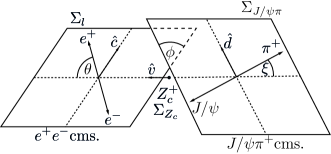
Figure 7: Choice of kinematical variables in the four-particle decay $Z_{c}^{+}\to{J/\psi}\pi^{+}\ell^{+}\ell^{-}$.

To calculate the decay rates we have to specify two independent kinematical variables for the three-body decay $Z_{c}^{+}\to{J/\psi}\pi^{+}\gamma$ and five independent ones for the four-body decay $Z_{c}^{+}\to{J/\psi}\pi^{+}\ell^{+}\ell^{-}$. For the three-body decay we choose the invariant Mandelstam variables as

$$s_{12} = (p_{1}+p_{2})^{2}\,,$$

$$s_{31} = (p_{1}+q)^{2}\,,$$

$$s_{32} = (p_{2}+q)^{2}\,,$$

$$s_{12}+s_{31}+s_{32} = m_{Z_{c}}^{2}+m_{J/\psi}^{2}+m_{\pi}^{2}+\delta m_{\gamma}^{2}\,,$$ (21)

where $\delta m_{\gamma}^{2}$ is a cutoff parameter for the phase-space integration to avoid the infrared bremsstrahlung singularity for $s_{31}\rightarrow m_{\pi}^{2}$ and $s_{12}\rightarrow m_{Z_{c}}^{2}$ [see Sec. IV for further discussion].

With these definitions we can express the scalar products between the momenta $p_{1},p_{2}$ and $q$ as

$$p_{1}\cdot p_{2} =\frac{1}{2}(s_{12}-m_{\pi}^{2}-m_{{J/\psi}}^{2})\,,$$

$$p_{1}\cdot q =\frac{1}{2}(s_{31}-m_{\pi}^{2}-\delta m_{\gamma}^{2})\,,$$ (22)

$$p_{2}\cdot q =\frac{1}{2}(m_{Z_{c}}^{2}+m_{\pi}^{2}-s_{12}-s_{31})\,.$$

The scalar products between $p$ and one outgoing momentum can be eliminated due to momentum conservation. Now the phase space region of the three-body decay can be expressed through the following ranges for the kinematical variables Byckling:1973 :

$$(m_{\pi}+\delta m_{\gamma})^{2} \leq s_{31}\leq(m_{Z_{c}}-m_{J/\psi})^{2}\,,$$

$$s_{12}^{-} \leq s_{12}\leq s_{12}^{+}\,,$$ (23)

where

$$s_{12}^{\pm} =m_{J/\psi}^{2}+m_{\pi}^{2}$$

$$-\frac{1}{2s_{31}}\left[(s_{31}-m_{Z_{c}}^{2}+m_{J/\psi}^{2})(s_{31}+m_{\pi}^{2}-\delta m_{\gamma}^{2}\right.)$$

$$\mp\left.\lambda^{1/2}(s_{31},m_{Z_{c}}^{2},m_{J/\psi}^{2})\lambda^{1/2}(s_{31},m_{\pi}^{2},\delta m_{\gamma}^{2})\right]$$ (24)

and $\lambda(x,y,z)=x^{2}+y^{2}+z^{2}-2(xy+xz+yz)$ is the Källen triangle kinematical function.

To calculate the scalar products between the momentum vectors $p_{1},p_{2},k_{3}$ and $k_{4}$ we will consider three reference frames for the four particle phase space: the rest frame $\Sigma_{Z_{c}}$ of the $Z_{c}$ meson, the dilepton center-of-mass frame $\Sigma_{l}$, and the center-of-mass frame $\Sigma_{J/\psi\pi}$ of the ${J/\psi}~{}\pi$-pair [see Fig. 7]. For the four-body decay we choose the kinematical variables suggested in Ref. Cabibbo:1965zzb and extensively used e.g. in Refs. Bijnens:1992mk -Knochlein:1996ah :

• $s_{12}$, the invariant mass squared of the ${J/\psi}~{}\pi$-pair

• $s_{34}$, the invariant mass squared of the lepton pair

• $\theta$, the angle of the antilepton $l^{+}$ in $\Sigma_{l}$ with momentum $k_{3}$ and with respect to the dilepton line of flight in $\Sigma_{Z_{c}}$

• $\xi$, the angle of the pion $\pi^{+}$ in $\Sigma_{J/\psi\pi}$ with momentum $p_{1}$ and with respect to the dimeson line of flight in $\Sigma_{Z_{c}}$

• $\phi$, the angle between the plane formed by the mesons ${J/\psi}$, $\pi$ in $\Sigma_{Z_{c}}$ and the corresponding plane formed by the dileptons

It proves to be very helpful to introduce linear combinations of the momenta $p,p_{1},p_{2},k_{3}$ and $k_{4}$. One of these momenta can always be eliminated due to momentum conservation:

$$K =p_{1}+p_{2}\,, L=p_{1}-p_{2}\,,$$

$$Q =k_{3}+k_{4}\,, R=k_{3}-k_{4}\,.$$

In order to express the Lorentz scalar products in terms of the kinematical variables specified above, we need the following expressions with the general masses $M,m_{1},m_{2},m_{3},m_{4}$ (note that these expressions will hold for any four-body decay with the frames specified in Fig. 7)

$$K\cdot K =s_{12}\,,$$

$$Q\cdot Q =s_{34}\,,$$

$$K\cdot Q =\frac{1}{2}(M^{2}-s_{12}-s_{34})\,,$$

$$K\cdot L =m_{1}^{2}-m_{2}^{2}\,,$$

$$Q\cdot R =m_{3}^{2}-m_{4}^{2}\,,$$

$$Q\cdot L =\frac{(K\cdot L)}{(K\cdot K)}(K\cdot Q)+x\sigma_{12}\cos\xi\,,$$ (25)

$$K\cdot R =\frac{(Q\cdot R)}{(Q\cdot Q)}(K\cdot Q)+x\sigma_{34}\cos\theta\,,$$

$$R\cdot L =\frac{(Q\cdot R)}{(Q\cdot Q)}x\sigma_{12}\cos\xi+\frac{(K\cdot L)}{(K\cdot K)}x\sigma_{34}\cos\theta\,$$

$$+(K\cdot Q)\sigma_{12}\sigma_{34}\cos\xi\cos\theta+\frac{(Q\cdot R)}{(Q\cdot Q)}\frac{(K\cdot L)}{(K\cdot K)}(K\cdot Q)$$

$$-\sqrt{s_{12}s_{34}}\sigma_{12}\sigma_{34}\sin\xi\sin\theta\cos\phi$$

$$\sigma_{ij} =\frac{\lambda^{1/2}(s_{ij},m_{i}^{2},m_{j}^{2})}{s_{ij}},\quad x\,=\,\frac{1}{2}\lambda^{1/2}(M^{2},s_{12},s_{34})\,.$$

These relations are obtained by calculating the Lorentz boosts between the different frames $\Sigma_{l}$, $\Sigma_{J/\psi\pi}$ and $\Sigma_{Z_{c}}$ as done in Daphne:1992 . Now all scalar products between the outgoing momenta occurring in the spin-averaged amplitude $\sum_{\text{pol.}}\left|{\cal M}\right|^{2}$ for the four-body decay can be written as

$$p_{1}\cdot p_{2} = \frac{1}{2}(s_{12}-m_{1}^{2}-m_{2}^{2})\,,$$

$$k_{3}\cdot k_{4} = \frac{1}{2}(s_{34}-m_{3}^{2}-m_{4}^{2})\,,$$

$$p_{1}\cdot k_{3} = \frac{1}{4}(Q\cdot K+Q\cdot L+R\cdot K+R\cdot L)\,,$$

$$p_{2}\cdot k_{3} = \frac{1}{4}(Q\cdot K-Q\cdot L+R\cdot K-R\cdot L)\,,$$ (26)

$$p_{1}\cdot k_{4} = \frac{1}{4}(Q\cdot K+Q\cdot L-R\cdot K-R\cdot L)\,,$$

$$p_{2}\cdot k_{4} = \frac{1}{4}(Q\cdot K-Q\cdot L-R\cdot K+R\cdot L)\,.$$

The ranges of the variables, which define the limits of the phase-space integration, are

$$(m_{3}+m_{4})^{2} \leq s_{34}\ \leq\ (M-m_{1}-m_{2})^{2}\,,$$

$$(m_{1}+m_{2})^{2} \leq s_{12}\ \leq\ (M-\sqrt{s_{34}})^{2}\,,$$ (27)

$$0 \leq \theta,\xi\ \leq\ \pi\,,$$

$$-\pi \leq \phi\ \leq\ \pi\,.$$

In our case we set $M=m_{Z_{c}}$, $m_{1}=m_{\pi}$, $m_{2}=m_{{J/\psi}}$, and $m_{3}=m_{4}=m_{l}$. The decay rates can then be written as (see, e.g., Byckling:1973 )

$$\Gamma_{3}(Z_{c}^{+}\to{J/\psi}\pi^{+}\gamma)=\frac{1}{N_{3}}\int ds_{31}\int ds_{12}\sum_{\text{pol.}}\left|{\cal T}\right|^{2}\,,$$

$$\Gamma_{4}(Z_{c}^{+}\to{J/\psi}\pi^{+}\ell^{+}\ell^{-})=\frac{1}{N_{4}}\int ds_{34}\int ds_{12}$$

$$\times \int d\cos\theta\,d\cos\xi\,d\phi\,xs\sigma_{12}\sigma_{34}\sum_{\text{pol.}}\left|{\cal M}\right|^{2}\,,$$

where $N_{3}=3\times 2^{8}\pi^{3}m_{Z_{c}}^{3}$ and $N_{4}=3\times 2^{15}\pi^{6}m_{Z_{c}}^{3}$.

IV Numerical results

With the phenomenological Lagrangians, kinematics and partial evaluation of the transition amplitudes introduced we now can proceed to determine the widths of the three- and four-body decays numerically.

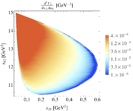
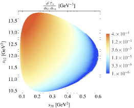
Figure 8: Double differential decay rate $d^{2}\Gamma_{3}/ds_{12}ds_{31}$ in $\mathrm{GeV^{-3}}$ for the three-body decay $Z_{c}^{+}\to{J/\psi}\pi^{+}\gamma$ ($\epsilon=3\mathrm{MeV}$ and $\Lambda=650\mathrm{MeV}$).

Figure 9: Double differential decay rate $d^{2}\Gamma_{3}/ds_{12}ds_{31}$ in $\mathrm{GeV^{-3}}$ for the three-body decay $Z_{c}^{+}\to{J/\psi}\pi^{+}\gamma$ ($\epsilon=3\mathrm{MeV}$ and $\Lambda=650\mathrm{MeV}$). The contour is nearly the same as in Fig. 9 except for $s_{31}\rightarrow m_{\pi}^{2}$ and $s_{12}\rightarrow m_{Z_{c}}^{2}$ where the bremsstrahlung singularity is located. This area is now excluded with an energy cut at $\delta m_{\gamma}=150\mathrm{MeV}$.

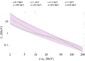
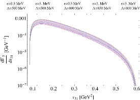
Figure 10: Partial decay rate $\Gamma_{3}$ in $\mathrm{MeV^{-1}}$ as a function of $\delta m_{\gamma}$ for selected values of $\epsilon$ and $\Lambda$ for the three-body decay $Z_{c}^{+}\to{J/\psi}\pi^{+}\gamma$.

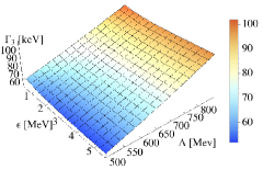
Figure 11: Differential decay rate $d\Gamma_{3}/ds_{31}$ in $\mathrm{GeV^{-1}}$ for selected values of $\epsilon$ and $\Lambda$ for the three-body decay $Z_{c}^{+}\to{J/\psi}\pi^{+}\gamma$ with $\delta m_{\gamma}=150\mathrm{MeV}$.

Figure 12: Partial decay rate $\Gamma_{3}$ in $\mathrm{keV}$ in dependence on $\epsilon$ and $\Lambda$ for the three-body decay $Z_{c}^{+}\to{J/\psi}\pi^{+}\gamma$ with $\delta m_{\gamma}=150\mathrm{MeV}$.

A full list of the results for the coupling $g_{Z_{c}}$ and the decay widths is tabulated in Appendix E. Table I contains the values for the coupling $g_{Z_{c}}$. In Tables II-IV we display the predictions for the three- and four-body decay rates for different values of the binding energy with $\epsilon=0.5\mathrm{MeV}$ to $5\mathrm{MeV}$ and of the cutoff in the vertex function with $\Lambda=500\mathrm{MeV}$ to $800\mathrm{MeV}$. A substantial increase of the size parameter $\Lambda$, more suitable for a compact bound state, would lead to a sizable increase in the decay rates. Therefore, if experiment will deliver larger values for the decay rates than predicted in our approach, this could signal that the $Z_{c}^{+}$ is probably not a molecular state.

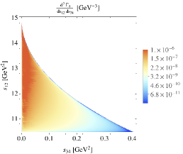
Figure 13: Double differential decay rate $d^{2}\Gamma_{4}/ds_{12}ds_{34}$ in $\mathrm{GeV^{-3}}$ for $\epsilon=3\mathrm{MeV}$ and $\Lambda=650\mathrm{MeV}$ for the four-body decay $Z_{c}^{+}\to{J/\psi}\pi^{+}e^{+}e^{-}$.

Figure 14: Double differential decay rate $d^{2}\Gamma_{4}/ds_{12}ds_{34}$ in $\mathrm{GeV^{-3}}$ for $\epsilon=3\mathrm{MeV}$ and $\Lambda=650\mathrm{MeV}$ for the four-body decay $Z_{c}^{+}\to{J/\psi}\pi^{+}\mu^{+}\mu^{-}$.

Let us first discuss the Dalitz plot $d^{2}\Gamma/ds_{12}ds_{31}$ for the three-body transition $Z_{c}^{+}\to{J/\psi}\pi^{+}\gamma$. The contour plot in Fig. 9 shows an infrared bremsstrahlung singularity for the limits $s_{31}\rightarrow m_{\pi}^{2}$ and $s_{12}\rightarrow m_{Z_{c}}^{2}$. For these values of $s_{31}$ and $s_{12}$ the bremsstrahlung diagrams $4$a, $4$b, $5$a and $5$b in Figs. 6 and 6 will generate a divergence in the double differential decay rate $d^{2}\Gamma/ds_{12}ds_{31}$.

A measurement of the partial or differential decay rate depends on the minimum photon energy detectable in the experimental facility. Hence, both in experiment and in theory, it is only possible to determine the partial or differential decay rate as a function of an energy cut $\delta m_{\gamma}$. To handle the bremsstrahlung singularity for $s_{31}\rightarrow m_{\pi}^{2}$ and $s_{12}\rightarrow m_{Z_{c}}^{2}$ we will use an energy cut at $\delta m_{\gamma}=150\mathrm{MeV}$ which holds for most facilities. When we apply the energy cut to the Dalitz plot in Fig. 9 we obtain Fig. 9 which has no bremsstrahlung singularity any more. In Fig. 12 we show the partial decay rate for the three-body transition $Z_{c}^{+}\to{J/\psi}\pi^{+}\gamma$ as a function of $\delta m_{\gamma}$. In Fig. 12 we give the differential decay rate $d\Gamma_{3}/ds_{31}$ which has been evaluated from $d^{2}\Gamma_{3}/ds_{12}ds_{31}$ by integration over $s_{12}$ for an energy cut at $\delta m_{\gamma}=150\mathrm{MeV}$.

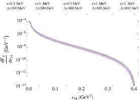
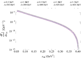
Figure 15: Differential decay rate $d\Gamma_{4}/ds_{34}$ in $\mathrm{GeV^{-1}}$ for selected values of $\epsilon$ and $\Lambda$ for the four-body decay $Z_{c}^{+}\to{J/\psi}\pi^{+}e^{+}e^{-}$.

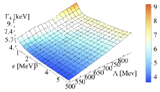
Figure 16: Differential decay rate $d\Gamma_{4}/ds_{34}$ in $\mathrm{GeV^{-1}}$ for selected values of $\epsilon$ and $\Lambda$ for the four-body decay $Z_{c}^{+}\to{J/\psi}\pi^{+}\mu^{+}\mu^{-}$.

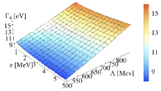
Figure 17: Partial decay rate $\Gamma_{4}$ in $\mathrm{keV}$ as a function of $\epsilon$ and $\Lambda$ for the four-body decay $Z_{c}^{+}\to{J/\psi}\pi^{+}e^{+}e^{-}$.

Figure 18: Partial decay rate $\Gamma_{4}$ in $\mathrm{keV}$ as a function of $\epsilon$ and $\Lambda$ for the four-body decay $Z_{c}^{+}\to{J/\psi}\pi^{+}\mu^{+}\mu^{-}$.

In Fig. 12 we demonstrate the sensitivity of the decay rate $\Gamma_{3}$ on variations of the free parameters $\epsilon$ and $\Lambda$ for an energy cut at $\delta m_{\gamma}=150\mathrm{MeV}$. We note that the dependence is rather flat, the decay rate does not change significantly under the considered variations of $\epsilon$ and $\Lambda$.

To avoid the bremsstrahlung singularity for $s_{31}\rightarrow m_{\pi}^{2}$ and $s_{12}\rightarrow m_{Z_{c}}^{2}$, another physics possibility is available: a lepton-antilepton pair can be attached to the photon line as described in Sec. II. Although the phase-space treatment for the four-body decays $Z_{c}^{+}\to{J/\psi}\pi^{+}e^{+}e^{-}$ and $Z_{c}^{+}\to{J/\psi}\pi^{+}\mu^{+}\mu^{-}$ gets more complicated, now an energy cut $\delta m_{\gamma}$ is not needed, the differential decay rates do not diverge. For the typical values of $\epsilon=3\mathrm{MeV}$ and $\Lambda=650\mathrm{MeV}$ we obtain the Dalitz plots $d^{2}\Gamma_{4}/ds_{12}ds_{34}$ depicted in Figs. 14 and 14 for the four-body decays $Z_{c}^{+}\to{J/\psi}\pi^{+}e^{+}e^{-}$ and $Z_{c}^{+}\to{J/\psi}\pi^{+}\mu^{+}\mu^{-}$.

The differential decay rates $d\Gamma_{4}/ds_{34}$, which have been evaluated from $d^{2}\Gamma_{4}/ds_{12}ds_{34}$ by integration over $s_{12}$, are displayed in Figs. 18 and 18. We demonstrate the sensitivity of the decay rates $\Gamma_{4}$ on variations of the free parameters $\epsilon$ and $\Lambda$ in Figs. 18 and 18. Here again, the decay rates do not change significantly under variations of $\epsilon$ and $\Lambda$.

V Summary

We have discussed the three- and four-body decays $Z_{c}^{+}\to{J/\psi}\pi^{+}\gamma$ and $Z_{c}^{+}\to{J/\psi}\pi^{+}\ell^{+}\ell^{-}$ of the $Z_{c}^{+}(3900)$ considered as a hadronic $\bar{D}D^{*}$ molecule in a phenomenological Lagrangian approach. Our approach is manifestly Lorentz and gauge invariant and is based on the use of the compositeness condition. We have only two model parameters: the binding energy $\epsilon$ and $\Lambda$, which is related to the size of the $\bar{D}D^{*}$ distribution in the $Z_{c}^{+}$-meson and, therefore, controls finite-size effects. The detailed results given for these decays are typical for a molecular state. A naive estimate for a compact configuration would correspond to considerably larger values of $\Lambda$ leading to a sizable enhancement of these decay rates. But this effect should be confirmed by an explicit calculation of the decay modes for a tetraquark interpretation of the $Z_{c}^{+}$.

To summarize, when interpreting the $Z_{c}^{+}$ as a $\bar{D}D^{*}$ molecule the resulting values for the decay widths are $50$-$100\mathrm{keV}$ for the transition $Z_{c}^{+}\to{J/\psi}\pi^{+}\gamma$, $4$-$10\mathrm{keV}$ for $Z_{c}^{+}\to{J/\psi}\pi^{+}e^{+}e^{-}$ and $8$-$16\mathrm{eV}$ for the decay $Z_{c}^{+}\to{J/\psi}\pi^{+}\mu^{+}\mu^{-}$. The predictions given here can add to the understanding of the $Z_{c}^{+}$ structure once the decay modes become accessible experimentally.

To elaborate further on a possible molecular structure of the $Z_{c}^{+}(3900)$ in future we plan to examine the transition $Z_{c}^{{}^{\prime}+}\to{J/\psi}\pi^{+}\gamma$ and $Z_{c}^{{}^{\prime}+}\to{J/\psi}\pi^{+}\ell^{+}\ell^{-}$ for the possible partner state $Z_{c}^{{}^{\prime}+}(3900)$, which is treated as a $\bar{D^{*}}D^{*}$ molecule Dong:2013iqa . As another possible continuation of this work $Z_{c}^{+}$ decays can also be studied in the tetraquark model Dubnicka:2010kz . This approach is also based on the compositeness condition and was successfully applied to the study of the $X(3872)$ as a possible tetraquark state. A full treatment of these observables for various structure interpretations can possibly help to understand the nature of these unusual meson states.

Appendix A Mass operator and coupling constant

The expressions for the coupling constant $g_{{}_{Z_{c}}}$ is

$$g_{Z_{c}}^{-2} = \Sigma_{\perp}^{\prime}(m_{Z_{c}}^{2})=\frac{m_{Z_{c}}^{2}}{32\pi^{2}}\int_{0}^{\infty}dxdy\frac{l}{a^{3}}\left(1+\frac{1}{2m_{D^{\ast}}^{2}a}\right)$$ (29)

$$\times \exp\left(m_{Z_{c}}^{2}\frac{l}{2a}-m_{D}^{2}x-m_{D^{\ast}}^{2}y\right)\,,$$

where $a=2s+x+y,l=sx+sy+2xy,s=\Lambda^{-2}$.

The numerical values are given in Table I.

Appendix B Feynman rules

Since nonlocal gauge theories are not so common, we will briefly indicate the relevant Feynman rules in this Appendix. In our calculations we use

$$D^{\mu\nu}(k) = \frac{i\biggl{(}-g^{\mu\nu}+\frac{k^{\mu}k^{\nu}}{M_{V}^{2}}\biggr{)}}{k^{2}-M_{V}^{2}}\ \approx\ -\frac{ig^{\mu\nu}}{k^{2}-M_{V}^{2}}$$

$$S(k) = \frac{i}{k^{2}-M_{S}^{2}}$$ (30)

for the vector and scalar propagators, respectively. The previously discussed arbitrary parameters $w_{1}$ and $w_{2}$ are now constrained to $w_{1}=w_{2}=1/2$. The vertex factors can be easily found by calculating the derivative of the Fourier transformed action of the corresponding diagram with respect to the fields which are attached to the vertex

$$i\Gamma_{n}(p_{1},p_{2},...,p_{n})=\left.\frac{i\delta^{n}S_{I}[\Phi]}{\delta\tilde{\Phi}_{1}(p_{1})\delta\tilde{\Phi}_{2}(p_{2})...\delta\tilde{\Phi}_{n}(p_{n})}\right|_{\tilde{\Phi}_{i}=0}.$$ (31)

The relevant vertices are denoted in Fig. 19. One finds for the vertex factors by dropping the usual factor $(2\pi)^{4}\delta^{4}(\sum P_{\text{in}}-\sum P_{\text{out}})$:

$$\text{(V1):}\,\,i\Gamma =\frac{-ig_{Z_{c}}}{\sqrt{2}}m_{Z_{c}}\Phi(-z_{1})g^{\alpha\mu}$$

$$\text{(V2):}\,\,i\Gamma =\frac{ig_{Z_{c}}}{2\sqrt{2}}m_{Z_{c}}e\,(p_{1}+p_{2}+q/2)^{\rho}g^{\alpha\mu}$$

$$\,\times\int\limits_{0}^{1}dt\Phi^{\prime}(-z_{2}t-z_{1}(1-t))$$

$$\text{(V3):}\,\,i\Gamma =ie\left[g^{\mu\nu}(p_{1}+p_{2})^{\rho}-g^{\mu\rho}p_{1}^{\nu}-g^{\nu\rho}p_{2}^{\mu}\right]$$

$$\approx ie\,(p_{1}+p_{2})^{\rho}g^{\mu\nu}$$

$$\text{(V4):}\,\,i\Gamma =-ie\,(p_{1}+p_{2})^{\rho}$$

$$\text{(V5):}\,\,i\Gamma =-ig_{DD^{\ast}J/\psi\pi}\,\sqrt{2}\,(p_{2}\cdot p_{1}g^{\mu\beta}-p_{2}^{\mu}p_{1}^{\beta})$$

$$\text{(V6):}\,\,i\Gamma =ig_{DD^{\ast}J/\psi\pi}\,e\sqrt{2}\,(g^{\mu\beta}p_{2}^{\rho}-p_{2}^{\mu}g^{\beta\rho})$$

where $z_{1}=(p_{1}/2+p_{2}/2)^{2}$ , $z_{2}=(q/2+p_{1}/2+p_{2}/2)^{2}$.

Appendix C Gauge invariance

In this Appendix we demonstrate that gauge invariance is fulfilled for the transition amplitude of the three-body decay $Z_{c}^{+}\to{J/\psi}\pi^{+}\gamma$. The $\bar{D}^{0*}D^{+}$-meson loop integrals corresponding to the diagrams in Fig. 6 are given by (we drop the general constant $c=-\frac{i}{16\pi^{2}}g_{Z_{c}}\,m_{Z_{c}}\,g_{DD^{\ast}J/\psi\pi}\,e$)

$$iI_{1a} =-\left(g^{\alpha\beta}p_{2}^{\rho}-p_{2}^{\alpha}g^{\beta\rho}\right)\int\frac{d^{4}k}{\pi^{2}i}\Phi(-k^{2})\tilde{S}(k+p/2)\tilde{D}(k-p/2)$$

$$iI_{2a} =-\left(p_{2}\cdot p_{1}g^{\alpha\beta}-p_{2}^{\alpha}p_{1}^{\beta}\right)\int\frac{d^{4}k}{\pi^{2}i}\Phi(-k^{2})\tilde{S}(k+p/2)\tilde{S}(k+p/2-q)\tilde{D}(k-p/2)(2k+p-q)^{\rho}$$

$$iI_{3a} =\left(p_{2}\cdot p_{1}g^{\alpha\beta}-p_{2}^{\alpha}p_{1}^{\beta}\right)\int_{0}^{1}dt\int\frac{d^{4}k}{\pi^{2}i}(k+3/4q)^{\rho}\Phi^{\prime}(-(k+q)^{2}t-(k+q/2)^{2}(1-t))\tilde{D}(k-p/2+q)\tilde{S}(k+p/2)$$

$$iI_{4a} =-\left((p-p_{2})\cdot p_{2}g^{\alpha\beta}-p_{2}^{\alpha}(p-p_{2})^{\beta}\right)(2p_{1}+q)^{\rho}\int\frac{d^{4}k}{\pi^{2}i}\Phi(-k^{2})\tilde{S}(k+p/2)\tilde{D}(k-p/2)\tilde{S}_{\pi}(p-p_{2})$$

$$iI_{5a} =-\left(p_{2}\cdot p_{1}g^{\alpha\beta}-p_{2}^{\alpha}p_{1}^{\beta}\right)(2p-q)^{\rho}\int\frac{d^{4}k}{\pi^{2}i}\Phi(-k^{2})\tilde{S}(k+p/2-q/2)\tilde{D}(k-p/2+q/2)\tilde{D}_{Z_{c}}(p-q)$$

where $k$ is the loop momentum and

$$\tilde{S}_{\pi}(k) =\frac{1}{m_{\pi}^{2}-k^{2}},\,\, \tilde{D}_{Z_{c}}(k)=\frac{1}{m_{Z_{c}}^{2}-k^{2}},$$

$$\tilde{S}(k) =\frac{1}{m_{D}^{2}-k^{2}},\,\, \tilde{D}(k)=\frac{1}{m_{D^{\ast}}^{2}-k^{2}},$$

are the propagators of the scalar and vector fields, respectively. As was already mentioned, the transverse parts of the vector propagators are neglected.

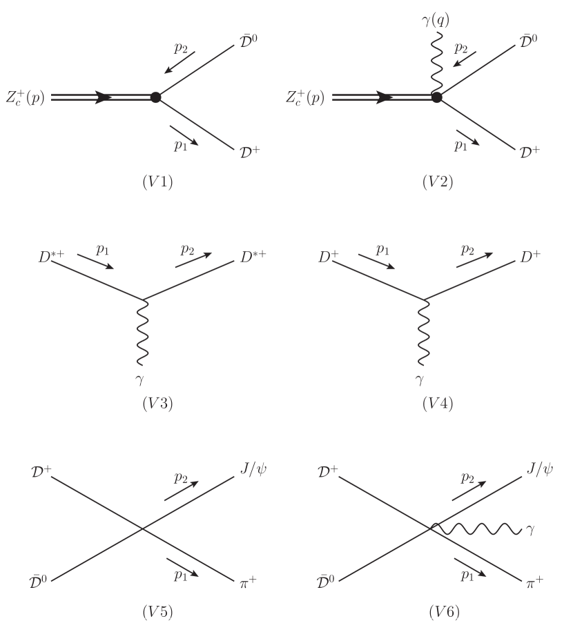
Figure 19: Vertices contributing to the three-body decay $Z_{c}^{+}\to{J/\psi}\pi^{+}\gamma$.

To test for gauge invariance every loop diagram is contracted with the photon momentum $q$. In the following it will be helpful to establish the following relations by taking advantage of momentum conservation $p=p_{1}+p_{2}+q$:

$$q\cdot(2k+p-q) = (k+p/2)^{2}-(k+p/2-q)^{2}$$

$$= \tilde{S}^{-1}(k+p/2-q)$$

$$-\tilde{S}^{-1}(k+p/2)$$ (33)

$$q\cdot(2p_{1}+q) = -\tilde{S}_{\pi}^{-1}(p-p_{2})$$ (34)

$$q\cdot(2p-q) = \tilde{D}_{Z_{c}}^{-1}(p_{1}+p_{2}).$$ (35)

Multiplying diagram $iI_{1a}$ with $q$ we get

$$qiI_{1a}=-\left(g^{\alpha\beta}q\cdot p_{2}-p_{2}^{\alpha}q^{\beta}\right)$$

$$\int\frac{d^{4}k}{\pi^{2}i}\Phi(-k^{2})\tilde{S}(k+p/2)\tilde{D}(k-p/2).$$ (36)

For the contraction of $iI_{2a}$ with $q$ and using (33) we obtain

$$qiI_{2a}=-\left(p_{2}\cdot p_{1}g^{\alpha\beta}-p_{2}^{\alpha}p_{1}^{\beta}\right)\int\frac{d^{4}k}{\pi^{2}i}\Phi(-k^{2})$$

$$\tilde{D}(k-p/2)\left[\tilde{S}(k+p/2)-\tilde{S}(k+p/2-q)\right].$$ (37)

Diagram $iI_{3a}$ multiplied with $q$ reads as

$$qiI_{3a} = \left(p_{2}\cdot p_{1}g^{\alpha\beta}-p_{2}^{\alpha}p_{1}^{\beta}\right)\int\frac{d^{4}k}{\pi^{2}i}\Phi(-k^{2})$$ (38)

$$\times \left[\tilde{D}(k-p/2+q/2)\tilde{S}(k+p/2-q/2)\right.$$

$$- \left.\tilde{D}(k-p/2)\tilde{S}(k+p/2-q)\right]$$

where we have used

$$\int_{0}^{1}dt\,q\cdot(k+3/4q)\Phi^{\prime}(-(k+q)^{2}t-(k+q/2)^{2}(1-t))$$

$$=-\Phi(-(k+q)^{2})+\Phi(-(k+q/2)^{2})\,.\hskip 28.45274pt$$

Furthermore we have shifted the first term of the integral containing the latter expression by $k\rightarrow k-q$ and the second term by $k\rightarrow k-q/2$. When multiplying $iI_{4a}$ with $q$ we obtain with the help of (34) and using momentum conservation

$$qiI_{4a}=\left((p_{1}+q)\cdot p_{2}g^{\alpha\beta}-p_{2}^{\alpha}(p_{1}+q)^{\beta}\right)$$

$$\int\frac{d^{4}k}{\pi^{2}i}\Phi(-k^{2})\tilde{S}(k+p/2)\tilde{D}(k-p/2).$$ (39)

We get the last expression with (35) and by multiplying $iI_{5a}$ with $q$

$$qiI_{5a}=-\left(p_{2}\cdot p_{1}g^{\alpha\beta}-p_{2}^{\alpha}p_{1}^{\beta}\right)\int\frac{d^{4}k}{\pi^{2}i}\Phi(-k^{2})$$

$$\tilde{S}(k+p/2-q/2)\tilde{D}(k-p/2+q/2).$$ (40)

Now it is easy to show that the expressions (C) to (C) cancel

$$q\left(iI_{1a}+iI_{2a}+iI_{3a}+iI_{4a}+iI_{5a}\right)=0.$$ (41)

Thus gauge invariance for the $\bar{D}^{0*}D^{+}$-meson loop integrals of Fig. 6 is shown. The proof of gauge invariance for the $\bar{D}^{0}D^{*+}$ loop diagrams of Fig. 6 proceeds exactly the same way as for the previous case of the $\bar{D}^{0*}D^{+}$-meson loop integrals by inserting the replacements $\tilde{S}(k)\leftrightarrow\tilde{D}(k)$.

Appendix D Structure integrals

In this Appendix the structure integrals $F_{1}$, $F_{235}\equiv F_{2}+F_{3}+F_{5}$ and $F_{4}$ are explicitly listed.
We define $c\equiv ig_{Z_{c}}\,m_{Z_{c}}\,g_{DD^{\ast}J/\psi\pi}\,e/(16\pi^{2})$, $s\equiv\Lambda^{-2}$ and $Q\equiv q$ for the three-body decay $Z_{c}^{+}\to{J/\psi}\pi^{+}\gamma$ and $Q\equiv k_{3}+k_{4}$ for the four-body decay $Z_{c}^{+}\to{J/\psi}\pi^{+}l^{+}l^{-}$.

$$iF_{1}=2c\int_{0}^{\infty}dxdy\frac{e^{-r_{1}^{2}/a_{1}-M_{1}^{2}}}{a_{1}^{2}}$$

$$r_{1} = p(s/2+y)$$

$$a_{1} = s+x+y$$

$$M_{1}^{2} = -m_{Z_{c}}^{2}(s/4+y)+m_{D}^{2}y+m_{D^{\ast}}^{2}x$$

$$iF_{2}=c\int_{0}^{\infty}dxdydz\frac{s+2z}{a_{2}^{3}}e^{-r_{2}^{2}/a_{2}}$$

$$\times\left(e^{-M_{2a}^{2}}+e^{-M_{2b}^{2}}\right)$$

$$r_{2} = p(s/2+z)+Qy$$

$$a_{2} = s+x+y+z$$

$$M_{2a}^{2} = -m_{Z_{c}}^{2}(s/4+z)+m_{D}^{2}(x+y)$$

$$+m_{D^{\ast}}^{2}z-Q^{2}\,y$$

$$M_{2b}^{2} = -m_{Z_{c}}^{2}(s/4+z)+m_{D^{\ast}}^{2}(x+y)$$

$$+m_{D}^{2}z-Q^{2}\,y$$

$$iF_{3}=-c\int_{0}^{\infty}dxdy\int_{0}^{1}dt\frac{s(x-y)}{2a_{3}^{3}}e^{-r_{3}^{2}/a_{3}}$$

$$\times\left(e^{-M_{3a}^{2}}+e^{-M_{3b}^{2}}\right)$$

$$r_{3} = \frac{1}{4}Q\left(s(2t-1)-3x+y\right)+\frac{1}{2}p(x-y)$$

$$a_{3} = s+x+y$$

$$M_{3a}^{2} = (4p\cdot Q(3x+y)-Q^{2}(s+9x+y)+$$

$$4(4m_{D}^{2}x+4m_{D^{\ast}}^{2}y-p^{2}(x+y)))/16$$

$$M_{3b}^{2} = (4p\cdot Q(3x+y)-Q^{2}(s+9x+y)+$$

$$4(4m_{D^{\ast}}^{2}x+4m_{D}^{2}y-p^{2}(x+y)))/16$$

$$iF_{4}=4c\int_{0}^{\infty}dxdy\frac{e^{-r_{4}^{2}/a_{4}-M_{4}^{2}}}{a_{4}^{2}}$$

$$\times\frac{1}{m_{\pi}^{2}-(p_{1}+Q)^{2}}$$

$$r_{4} = p(s/2+y)$$

$$a_{4} = s+x+y$$

$$M_{4}^{2} = -m_{Z_{c}}^{2}(s/4+y)+m_{D}^{2}y+m_{D^{\ast}}^{2}x$$

$$iF_{5}=4c\int_{0}^{\infty}dxdy\frac{e^{-r_{5}^{2}/a_{5}-M_{5}^{2}}}{a_{5}^{2}}$$

$$\times\frac{1}{m_{Z}^{2}-(p_{1}+p_{2})^{2}}$$

$$r_{5} = p(s/2+x)+Q(s/2+y)$$

$$a_{5} = s+x+y$$

$$M_{5}^{2} = -m_{Z_{c}}^{2}(s/4+x)+m_{D^{\ast}}^{2}x+m_{D}^{2}y$$

$$-p\cdot Q\,s/2-Q^{2}\,(s/4+y)$$

Appendix E Numerical values

We summarize the numerical results for the coupling constant $g_{Z_{c}}$ and the decay rates $\Gamma_{3}$, $\Gamma_{4}$ of the three- and four-body transitions.

Table 1: Numerical values for the dimensionless phenomenological coupling constant $g_{Z_{c}}$ as a function of $\epsilon$ (column 1) and $\Lambda$ (row 1).

$\epsilon\backslash\Lambda$ [MeV]	500	550	600	650	700	750	800
0.5	6.23	5.95	5.71	5.52	5.35	5.21	5.09
1.0	6.36	6.07	5.83	5.62	5.45	5.31	5.18
1.5	6.49	6.19	5.94	5.73	5.55	5.40	5.27
2.0	6.62	6.31	6.05	5.83	5.65	5.49	5.36
2.5	6.75	6.43	6.16	5.93	5.74	5.58	5.44
3.0	6.88	6.54	6.27	6.03	5.84	5.67	5.53
3.5	7.01	6.66	6.37	6.13	5.93	5.76	5.61
4.0	7.13	6.77	6.48	6.23	6.03	5.85	5.70
4.5	7.26	6.89	6.58	6.33	6.12	5.94	5.78
5.0	7.38	7.00	6.69	6.43	6.21	6.02	5.86

Table 2: Numerical values for the decay rate $\Gamma_{3}$ in $\mathrm{keV}$ for the transition $Z_{c}^{+}\to{J/\psi}\pi^{+}\gamma$ for $\delta m_{\gamma}=150\mathrm{MeV}$ as a function of $\epsilon$ (column 1) and $\Lambda$ (row 1).

$\epsilon\backslash\Lambda$ [MeV]	500	550	600	650	700	750	800
0.5	61.1	67.4	73.9	80.5	87.5	94.7	101.9
1.0	58.1	64.2	70.8	77.5	84.5	91.7	99.2
1.5	56.1	62.5	69.0	75.7	82.9	90.2	97.7
2.0	54.9	61.3	67.9	74.8	81.8	89.3	96.8
2.5	54.0	60.4	67.1	74.1	81.2	88.6	96.3
3.0	53.3	59.8	66.5	73.6	80.8	88.3	96.1
3.5	52.8	59.3	66.2	73.3	80.6	88.3	96.0
4.0	52.4	59.1	65.9	73.1	80.6	88.1	96.1
4.5	52.1	58.8	65.8	73.0	80.5	88.3	96.3
5.0	51.9	58.7	65.7	73.0	80.6	88.4	96.5

Table 3: Numerical values for the decay rate $\Gamma_{4}$ in $\mathrm{keV}$ for the transition $Z_{c}^{+}\to{J/\psi}\pi^{+}e^{+}e^{-}$ as a function of $\epsilon$ (column 1) and $\Lambda$ (row 1).

$\epsilon\backslash\Lambda$ [MeV]	500	550	600	650	700	750	800
0.5	5.770	6.440	7.070	7.239	7.620	8.575	9.230
1.0	4.802	5.118	5.725	6.079	6.664	7.149	7.597
1.5	4.308	4.704	5.208	5.678	6.332	6.853	7.207
2.0	4.123	4.531	4.970	5.484	5.995	6.536	6.999
2.5	3.933	4.418	4.911	5.303	5.843	6.331	6.931
3.0	3.826	4.308	4.782	5.321	5.859	6.293	6.885
3.5	3.778	4.253	4.719	5.202	5.774	6.279	6.824
4.0	3.726	4.174	4.673	5.174	5.704	6.246	6.812
4.5	3.690	4.150	4.636	5.142	5.703	6.265	6.804
5.0	3.661	4.141	4.623	5.151	5.699	6.278	6.854

Table 4: Numerical values for the decay rate $\Gamma_{4}$ in $\mathrm{eV}$ for the transition $Z_{c}^{+}\to{J/\psi}\pi^{+}\mu^{+}\mu^{-}$ as a function of $\epsilon$ (column 1) and $\Lambda$ (row 1).

$\epsilon\backslash\Lambda$ [MeV]	500	550	600	650	700	750	800
0.5	9.593	10.559	11.574	12.621	13.711	14.826	15.986
1.0	9.080	10.064	11.079	12.130	13.216	14.352	15.515
1.5	8.779	9.7613	10.789	11.848	12.951	14.082	15.252
2.0	8.572	9.5626	10.587	11.664	12.775	13.922	15.105
2.5	8.415	9.4161	10.461	11.541	12.656	13.810	15.006
3.0	8.297	9.3083	10.360	11.453	12.584	13.750	14.955
3.5	8.206	9.2270	10.294	11.391	12.528	13.708	14.918
4.0	8.136	9.1672	10.237	11.349	12.493	13.683	14.906
4.5	8.084	9.1159	10.196	11.316	12.478	13.673	14.906
5.0	8.035	9.0827	10.165	11.300	12.466	13.675	14.920

References

- (1) M. Ablikim et al. [BESIII Collaboration], Phys. Rev. Lett. 110, 252001 (2013) [arXiv:1303.5949 [hep-ex]].
- (2) Z. Q. Liu et al. [Belle Collaboration], Phys. Rev. Lett. 110, 252002 (2013) [arXiv:1304.0121 [hep-ex]].
- (3) T. Xiao, S. Dobbs, A. Tomaradze and K. K. Seth, Phys. Lett. B 727, 366 (2013) arXiv:1304.3036 [hep-ex].
- (4) L. Maiani, V. Riquer, R. Faccini, F. Piccinini, A. Pilloni and A. D. Polosa, Phys. Rev. D 87, 111102 (2013) [arXiv:1303.6857 [hep-ph]].
- (5) J. M. Dias, F. S. Navarra, M. Nielsen and C. M. Zanetti, Phys. Rev. D 88, 016004 (2013) [arXiv:1304.6433 [hep-ph]].
- (6) E. Braaten, Phys. Rev. Lett. 111, 162003 (2013) [arXiv:1305.6905 [hep-ph]].
- (7) Q. Wang, C. Hanhart and Q. Zhao, Phys. Rev. Lett. 111, 132003 (2013) [arXiv:1303.6355 [hep-ph]].
- (8) C. Y. Cui, Y. L. Liu, W. B. Chen and M. Q. Huang, J. Phys. G 41, 075003 (2014) [arXiv:1304.1850 [hep-ph]].
- (9) J. R. Zhang, Phys. Rev. D 87, 116004 (2013) [arXiv:1304.5748 [hep-ph]].
- (10) H. W. Ke, Z. T. Wei and X. Q. Li, Eur. Phys. J. C 73, 2561 (2013) [arXiv:1307.2414].
- (11) Y. Dong, A. Faessler, T. Gutsche and V. E. Lyubovitskij, Phys. Rev. D 88, 014030 (2013) [arXiv:1306.0824 [hep-ph]].
- (12) Y. Dong, A. Faessler, T. Gutsche and V. E. Lyubovitskij, J. Phys. G 40, 015002 (2013) [arXiv:1203.1894 [hep-ph]].
- (13) Y. Dong, A. Faessler, T. Gutsche and V. E. Lyubovitskij, Phys. Rev. D 89, 034018 (2014) [arXiv:1310.4373 [hep-ph]].
- (14) A. Faessler, T. Gutsche, V. E. Lyubovitskij and Y. -L. Ma, Phys. Rev. D 76, 014005 (2007) [arXiv:0705.0254 [hep-ph]]; T. Branz, T. Gutsche and V. E. Lyubovitskij, Phys. Rev. D 80, 054019 (2009) [arXiv:0903.5424 [hep-ph]]; Phys. Rev. D 82, 054025 (2010) [arXiv:1005.3168 [hep-ph]]; Phys. Rev. D 78, 114004 (2008) [arXiv:0808.0705 [hep-ph]]; Y. B. Dong, A. Faessler, T. Gutsche and V. E. Lyubovitskij, Phys. Rev. D 77, 094013 (2008) [arXiv:0802.3610 [hep-ph]]; Y. Dong, A. Faessler, T. Gutsche and V. E. Lyubovitskij, arXiv:1404.6161 [hep-ph].
- (15) Y. Dong, A. Faessler, T. Gutsche and V. E. Lyubovitskij, J. Phys. G 38, 015001 (2011) [arXiv:0909.0380 [hep-ph]];
- (16) S. Weinberg, Phys. Rev. 130, 776 (1963).
- (17) G. V. Efimov and M. A. Ivanov, The Quark Confinement Model of Hadrons, (IOP Publishing, Bristol Philadelphia, 1993)
- (18) T. Branz, A. Faessler, T. Gutsche, M. A. Ivanov, J. G. Korner and V. E. Lyubovitskij, Phys. Rev. D 81, 034010 (2010) [arXiv:0912.3710 [hep-ph]].
- (19) Y. Dong, A. Faessler, T. Gutsche and V. E. Lyubovitskij, Phys. Rev. D 81, 014006 (2010) [arXiv:0910.1204 [hep-ph]].
- (20) I. V. Anikin, M. A. Ivanov, N. B. Kulimanova and V. E. Lyubovitskij, Z. Phys. C 65, 681 (1995).
- (21) M. A. Ivanov, M. P. Locher and V. E. Lyubovitskij, Few-Body Syst. 21, 131 (1996) [hep-ph/9602372].
- (22) M. A. Ivanov, V. E. Lyubovitskij, J. G. Korner and P. Kroll, Phys. Rev. D 56, 348 (1997) [hep-ph/9612463].
- (23) A. Faessler, T. Gutsche, M. A. Ivanov, J. G. Korner and V. E. Lyubovitskij, Phys. Lett. B 518, 55 (2001) [hep-ph/0107205].
- (24) A. Faessler, T. Gutsche, M. A. Ivanov, J. G. Korner, V. E. Lyubovitskij, D. Nicmorus and K. Pumsa-ard, Phys. Rev. D 73, 094013 (2006) [hep-ph/0602193].
- (25) A. Faessler, T. Gutsche, B. R. Holstein, V. E. Lyubovitskij, D. Nicmorus and K. Pumsa-ard, Phys. Rev. D 74, 074010 (2006) [hep-ph/0608015].
- (26) S. Mandelstam, Ann. Phys. (N.Y.) 19, 1 (1962).
- (27) J. Terning, Phys. Rev. D 44, 887 (1991).
- (28) A. Faessler, T. Gutsche, M. A. Ivanov, V. E. Lyubovitskij and P. Wang, Phys. Rev. D 68, 014011 (2003) [hep-ph/0304031].
- (29) A. Faessler, T. Gutsche, V. E. Lyubovitskij and Y. -L. Ma, Phys. Rev. D 76, 114008 (2007) [arXiv:0709.3946 [hep-ph]].
- (30) A. Faessler, T. Gutsche, S. Kovalenko and V. E. Lyubovitskij, Phys. Rev. D 76, 1 (2007) [arXiv:0705.0892 [hep-ph]].
- (31) E. Byckling and K. Kajantie, Particle Kinematics, (Wiley, New York, 1973), p. 319.
- (32) N. Cabibbo and A. Maksymowicz, Phys. Rev. 137, B438 (1965); 168, 1926 [E] 1968.
- (33) J. Bijnens, G. Ecker and J. Gasser, in The DANE Physics Handbook, edited by L. Maiani, G. Pancheri, and N. Paver (Servizio Documentazione dei Laboratori Nazionali di Frascati, Frascati, 1992), Vol. I.
- (34) V.S. Demidov and E. Shabalin, in The DANE Physics Handbook, edited by L. Maiani, G. Pancheri, and N. Paver (Servizio Documentazione dei Laboratori Nazionali di Frascati, Frascati, 1992), Vol. I
- (35) J. Bijnens, Int. J. Mod. Phys. A 8 3045 (1993).
- (36) G. Knochlein, S. Scherer and D. Drechsel, Phys. Rev. D 53 (1996) 3634 [hep-ph/9601252].
- (37) S. Dubnicka, A. Z. Dubnickova, M. A. Ivanov and J. G. Korner, Phys. Rev. D 81, 114007 (2010) [arXiv:1004.1291 [hep-ph]]; S. Dubnicka, A. Z. Dubnickova, M. A. Ivanov, J. G. Korner, P. Santorelli and G. G. Saidullaeva, Phys. Rev. D 84, 014006 (2011) [arXiv:1104.3974 [hep-ph]].