ASKIT: Approximate Skeletonization Kernel-Independent Treecode in High Dimensions

Abstract

We present a fast algorithm for kernel summation problems in high-dimensions. Such problems appear in computational physics, numerical approximation, non-parametric statistics, and machine learning. In our context, the sums depend on a kernel function that is a pair potential defined on a dataset of points in a high-dimensional Euclidean space. A direct evaluation of the sum scales quadratically with the number of points. Fast kernel summation methods can reduce this cost to linear complexity, but the constants involved do not scale well with the dimensionality of the dataset.

The main algorithmic components of fast kernel summation algorithms are the separation of the kernel sum between near and far field (which is the basis for pruning) and the efficient and accurate approximation of the far field.

We introduce novel methods for pruning and for approximating the far field. Our far field approximation requires only kernel evaluations and does not use analytic expansions. Pruning is not done using bounding boxes but rather combinatorially using a sparsified nearest-neighbor graph of the input distribution. The time complexity of our algorithm depends linearly on the ambient dimension. The error in the algorithm depends on the low-rank approximability of the far field, which in turn depends on the kernel function and on the intrinsic dimensionality of the distribution of the points. The error of the far field approximation does not depend on the ambient dimension.

We present the new algorithm along with experimental results that demonstrate its performance. As a highlight, we report results for Gaussian kernel sums for 100 million points in 64 dimensions, for one million points in 1000 dimensions, and for problems in which the Gaussian kernel has a variable bandwidth. To the best of our knowledge, all of these experiments are prohibitively expensive with existing fast kernel summation methods.

1 Introduction

Given a set of $N$ points $\{{{x}}_{j}\}_{j=1}^{N}\in\mathbb{R}^{d}$ and weights $w_{j}\in\mathbb{R}$, we wish to compute

(1) $$u_{i}=u({{x}}_{i})=\sum_{j=1}^{N}K({{x}}_{i},{{x}}_{j})w_{j},\quad\forall i=1\ldots N.$$

Here $K()$, a given function, is the kernel. Equation 1 is the kernel summation problem, also commonly referred to as an N-body problem. From a linear algebraic viewpoint, kernel summation is equivalent to approximating ${{u}}={{{K}}}{{w}}$ where ${u}$ and ${w}$ are $N$-dimensional vectors and ${{K}}$ is a $N\times N$ matrix consisting of the pairwise kernel evaluations. From linear algebraic viewpoint, fast kernel summations can be viewed as hierarchical low-rank approximations for ${{K}}$.

Direct evaluation of the sum requires $\operatorname{\mathcal{O}}(N^{2})$ work. Fast kernel summations can reduce this cost dramatically. For $d=2$ and $d=3$ and for specific kernels, these algorithms are extremely efficient and can evaluate 1 in $\operatorname{\mathcal{O}}(N\log N)$ work (treecodes) or $\operatorname{\mathcal{O}}(N)$ work (fast multipole methods) to arbitrary accuracy [6, 13].

The main idea in accelerating (1) is to exploit low-rank blocks of the matrix ${{K}}$. These blocks are related to the smoothness of the underlying kernel function $K()$, which in turn is directly related to pairwise similarities between elements of a set, such as distances between points. Hierarchical data structures reveal these low rank blocks by rewriting (1) as

(2) $$u_{i}=\sum_{j\in\mathrm{Near}(i)}K_{ij}w_{j}+\sum_{j\in\mathrm{Far}(i)}K_{ij}w_{j},$$

where $\mathrm{Near}(i)$ is the set of points ${{x}}_{j}$ whose contributions cannot be approximated well by a low-rank scheme and $\mathrm{Far}(i)$ indicates the set of points ${{x}}_{j}$ whose contributions can. The first term is often referred to as the near field for the point ${{x}}_{i}$ and the second term is referred to as the far field. Throughout, we refer to a point ${{x}}_{i}$ for which we compute $u_{i}$ as a target and a point ${{x}}_{j}$ as a source. We fix a group of source points and use $K$ to represent the interaction of these source points with distant targets (here we abuse the notation, since $K$ is just a block of the original matrix). The low rank approximation used in treecodes and fast multipole methods is equivalent to a hierarchical low rank factorization of $K$.

The results, algorithms, and theory for the kernels in low dimensions can be readily extended to any arbitrary dimension, but the constants in the complexity estimates for both error and time do not scale well with $d$. For example, the Fast Multipole Method of Greengard and Rokhlin [12] scales exponentially with $d$. We are interested in developing a fast summation method that can be applied to points in an arbitrary dimension $d$—provided $K$ has a low-rank structure. To clarify, here we are not claiming to be generically addressing the fast summation for any kernel and any distribution of points. As $d$ increases we need to differentiate between the notion of the ambient dimension $d$ and the intrinsic dimension ${d_{\mathrm{intr}}}$ of the dataset. (For example, the intrinsic dimension of points sampled on a 3D curve is one.) Empirically, it has been observed that high-dimensional data are commonly embedded in some, generally unknown and non-planar, lower dimensional subspace. An efficient fast summation algorithm must be able to take advantage of this structure in order to scale well with both the ambient and intrinsic dimensions. Existing methods do not exploit such structure.

Outline of treecodes. Roughly speaking, fast summation algorithms for (1) can be categorized based on 1) how the Near$(i)$ and Far$(i)$ splittings are defined, and 2) the construction and evaluation of the low rank approximation of $K_{ij}$ (for $j\in\mathrm{Far}(i)$). First, we partition the input points using a space partitioning tree data structure (for example $kd$-trees). Then, to evaluate the sum for a query, we use special traversals of the tree. A treecode has the following simple structure (see Algorithm 1): for each target point, we group all the nodes of the tree into Near and Far sets. The interactions from Near nodes are evaluated directly and those from Far nodes are approximated from their approximate representations. Existing fast algorithms create the Near/Far groups based on some measure of the distance of a node from the target point. When a node is far apart or well-separated from a target, the algorithm terminates the tree traversal and evaluates the approximate interactions from the node to the target point. We refer to this termination as pruning and the distance-based schemes to group the nodes to Near and Far field as distance pruning.

The far field approximation. The far-field approximate representation for every node has been constructed during a preprocessing step. In a companion paper [23], we review the main methods for constructing far-field approximations, and we introduce the approximation we use here. We also review this approach in §2.

Shortcomings of existing methods. In high dimensions (e.g. $d>100$), most existing methods for constructing far field approximations fail because they become too expensive, they do not adapt to ${d_{\mathrm{intr}}}$, and distance pruning fails in high dimensions. Also, most schemes use analytic arguments to design the far-field and depend on the type or class of the kernel. Although there has been extensive work on these methods for classical kernels like the Gaussian, other kernels are also used such as kernels with variable bandwidth that are not shift invariant [29]. This observation further motivates the use of entirely algebraic acceleration techniques for (1).

Contributions

We present "ASKIT" (Approximate Skeletonization Kernel Independent Treecode), a fast kernel summation treecode with a new pruning scheme and a new far field low-rank representation. Our scheme depends on both the decay properties of the kernel matrix and the manifold structure of the input points. In a nutshell our contributions can be summarized as follows:

• Pruning or near field-far field node grouping. In ASKIT, pruning is not done using the usual distance/bounding box calculations. Instead, we use a combinatorial criterion based on nearest neighbors which we term neighbor pruning. Experimentally, this scheme improves pruning in high dimensions and opens the way to more generic similarity functions. Also, based on this decomposition, we can derive complexity bounds for the overall algorithm.

• Far field approximation. Our low rank far field scheme uses an approximate interpolative decomposition (ID) (for the exact ID see [21, 16]) which is constructed using nearest-neighbor sampling augmented with randomized uniform sampling. Our method enjoys several advantages over existing methods: it only requires kernel evaluations, rather than any prior knowledge of the kernel such as in analytic expansion-based schemes; it can evaluate kernels which depend on local structure, such as kernels with variable bandwidths; and its effectiveness depends only on the linear algebraic rank of sub-blocks of the kernel matrix and provides near-optimal (compared to SVD) compression without explicit dependence on the ambient dimension of the data. The basic notions for the far field were introduced in [23]. Here we introduce the hierarchical scheme, and evaluate its performance.

• Experimental evaluation. One commonly used kernel in statistical learning is the Gaussian kernel $K({{x}}_{i}-{{x}}_{j})=\exp(-\|{{x}}_{i}-{{x}}_{j}\|^{2}_{2}/\sigma_{j}^{2})$. We focus our experiments on this kernel and we test it on synthetic and scientific datasets. We also allow for a bandwidth that depends on the source or target point—the variable bandwidth case. We demonstrate the linear dependence on the ambient dimension by conducting an experiment with $d=1000$ (and ${d_{\mathrm{intr}}}=4$) in which the far field cannot be truncated and for which we achieve six digits of accuracy and a 20$\times$ speedup over direct $N^{2}$ evaluation. On a 5M-point, 18D UCI Machine Learning Repository [2] dataset, we obtain 25$\times$ speedup. On a 5M-point, 128D dataset, we obtain 2000$\times$ speedup using 4,096 x86 cores. Our largest run involved 100M points in 128D on 8,192 x86 cores.

In our experiments, we use Euclidean distances and classical binary space partitioning trees. We require nearest-neighbor information for every point in the input dataset. The nearest neighbors are computed using random projection trees [7] with greedy search (Section 2). Our implementation combines the Message Passing Interface (MPI) protocol for high-performance distributed memory parallelism and the OpenMP protocol for shared memory parallelism.

Limitations

The main limitation of our method is that the approximation rank (the skeleton size in §2) is selected manually and is fixed. In a black-box implementation for use by non-experts, this parameter needs to be selected automatically. The current algorithm also has the following parameters: the number of approximate nearest neighbor, the desired accuracy of approximation, the number of sampling points, and the number of points per box. The nearest neighbors have a more subtle effect on the overall scheme that can be circumvented with an adaptive choice of approximation rank. In our experiments, their number is fixed, but this could also be adaptive. The other parameters are easier to select, and they tend to affect the performance more than the accuracy of the algorithm. Furthermore, the error bounds that we present are derived for the case of uniform sampling and the analysis is not informative on how to use the various parameters. More accurate analysis can be done in a kernel-specific fashion. Another shortcoming of the method regards performance optimization. This is a first implementation of our scheme and it is not optimized. A fast-multipole variant of this method would also result in $\operatorname{\mathcal{O}}(N)$ complexity, but we defer this to future work.

Finally, let us mention a fundamental limitation of our scheme. Our far-field approximation requires that blocks of $K$ have low rank structure. The most accurate way to compute this approximation is using the singular value decomposition. There are kernels and point distributions for which point distance-based blocking of $K$ does not result in low-rank blocks. In that case, ASKIT will either produce large errors or it will be slower than a direct sum. Examples of such difficult to compress kernels are the (2$d$ or 3$d$) high frequency Helmholtz kernel [8] and in high intrinsic dimensions the Gaussian kernel (for certain bandwidths and point distributions) [23].

Related work

Originally, fast kernel summation methods were developed for problems in computational physics. The underlying kernels are related to fundamental solutions of partial differential equations (Green’s functions). Examples include the 3D Laplace potential (reciprocal distance kernel) and the heat potential (Gaussian kernel). Beyond computational physics, kernel summation can be used for radial basis function approximation methods. They also find application to non-parametric statistics and machine learning tasks such as density estimation, regression, and classification. Linear inference methods such as support vector machines [30] and dimension reduction methods such as principal components analysis [25] can be generalized to kernel methods [4], which in turn require fast kernel summation.

Seminal work for kernel summations in $d\leq 3$ includes [12, 6] and [13]. In higher dimensions related work includes [14, 11, 18, 26, 31]. One of the fastest schemes in high dimensions is the improved fast Gauss transform [31, 26]. In all these methods, the low rank approximation of the far field is based on analytic and kernel-specific expansions. The cost of constructing and evaluating these expansions scales either as $\operatorname{\mathcal{O}}(c^{d})$ (resulting in SVD-quality errors) or as $\operatorname{\mathcal{O}}(d^{c})$, where $c>0$ is related to the accuracy of the expansion. Except for very inaccurate approximations, $c>2$ and thus all of these schemes become extremely expensive with increasing $d$. In addition to the expensive scaling with ambient dimension, the approximations in these methods must be derived and implemented individually for each new kernel function.

An alternative class of methods is based on a hybrid of analytic arguments and algebraic approximations. Examples include [32, 9, 10]. However, these methods also scale as $\operatorname{\mathcal{O}}(c^{d})$ or worse [23]. We also mention methods which rely only on kernel evaluations and use spatial decomposition to scale with ${d_{\mathrm{intr}}}$ in which the far-field approximation is computed on the fly with exact error guarantees [11] or approximately using Monte Carlo methods [19]. However, these methods rely on distance-based pruning, which can fail in extremely high dimensions, and the randomized method is extremely slow to converge. Another scheme that only requires kernel evaluations (in the frequency domain) is [27]. But its performance depends on the ambient dimension and on the kernel being diagonalizable in Fourier space. For a more extensive discussion on the far field approximation that we use here and a more detailed review of the related literature, we refer the reader to our work [23].

Algebraic methods work with the matrix entries directly. One set of methods similar to the one presented here. uses a low-rank matrix decomposition of subblocks of the kernel matrix [24]. However, this method still requires interpolation points over a bounding surface, which scale poorly with $d$. Another collection of methods, generally called “adaptive cross approximation” methods, also make use of low-rank factorization of subblocks [3, 17, 33]. The linear scaling of these methods requires the ability to decompose the input points into large, well- separated sets, which will generally only be possible in low dimensions.

To the best of our knowledge, all existing treecodes use distance-based pruning, sometimes augmented with kernel evaluations to better control the error. Our scheme is the first to introduce an alternative pruning approach not based on kernel evaluations or bounding box-based distance calculations.

Since we present experimental results performed in parallel, we also mention another existing body of work on parallel treecodes [20]. However, our parallel algorithms are quite different (and our efficiency relies on neighbor pruning). The specifics will be reported elsewhere since the parallelization of ASKIT is not our main point here.

We use randomized tree searches to compute approximate nearest neighbors. There is a significant body of literature on such methods, but we do not discuss them further since our scheme does not depend on the details of the neighbor search (although it does depend on the approximation error, if the nearest neighbors have been computed approximately.) Representative works include [1] and [7]. We describe the method used in our experiments in §2.2.

2 Algorithms

$N$	number of points
$K$	the kernel function or matrix
$\kappa$	number of nearest neighbors per point
${m}$	number of points per leaf
${s}$	number of skeleton points
${{\mathcal{X}}}$	integer set $\{1,\ldots,N\}$
${\mathcal{X}}_{\alpha}$	ids of points in node $\alpha$
$\alpha$	tree node or simply node
$\alpha_{i}$	leaf node that contains point $i$
${{\mathcal{N}}_{i}}$	neighbor list for point $i$
${{\mathcal{N}}_{\alpha}}$	neighbor list for node $\alpha$
${\mathcal{A}}_{\alpha}$	ancestor list of node $\alpha$
${{\tt r}(\alpha)}$	right child of node $\alpha$
${{\tt l}(\alpha)}$	left child of node $\alpha$

Table 1: Here we summarize main notation used in the text. In addition to the information above, we use ${\,\cup\,}$ to indicate the set union of two index sets, ${\,\setminus\,}$ the difference of two index sets, and ${|\cdot|}$ the number of elements in set. We define IsLeaf($\alpha$) to be true if $\alpha$ is a leaf. We also use $w({\mathcal{I}})$ to indicate the components of vector $w$ determined by an index set ${\mathcal{I}}$ and we use a similar notation for matrices.

We now turn to the description of the new algorithm. We begin by summarizing the basic structure of a treecode. In a treecode, we first construct a tree that is used for space-partitioning of the input points. We use this term to broadly cover any hierarchical partitioning of the data set such that nearby (or similar) points are grouped together. For our purposes, a tree consists of internal nodes with two or more children and leaf nodes with no children.

Given such a tree, a treecode performs a two-stage computation to approximate the kernel summations. In the first stage, a bottom-up tree traversal takes place (also known as the upward pass) in which at each node we create a low-rank approximation of the far field generated by all the source points in it. We form these representations at the leaf nodes, then pass them up to parents and combine them in a recursive manner. In the second stage, a concurrent top-down traversal (also known as the downward pass) takes place in which we use these representations to compute approximate potentials. That is, for each target point $x$, we traverse the tree from the top down. At a node $\alpha$, we apply a pruning criterion to determine whether or not we can approximate the far-field generated from sources in $a$ and evaluated at $x$. If we can approximate it, then we use the low-rank approximation to evaluate the far field at $x$ and then we prune the tree traversal at the node $a$. If we cannot approximate it, we recurse and visit the children of $a$. If we still cannot prune at a leaf, we evaluate the contribution of the leaf’s points directly (no approximation takes place). If by ${\tilde{K}}$ we denote the approximate kernel (meaning that we use a low rank approximation), a template for a generic treecode is given by Algorithm 1.

Algorithm 1 Treecode(Target point $x$, Source tree node $a$)

  if we can approximate $u(x)=K(x,{\mathcal{X}}_{\alpha})w({\mathcal{X}}_{\alpha})$ then {using pruning criterion}

     return  $u(x)={\tilde{K}}_{a}(x)$

  else if $a$ is a leaf then

     return  $\sum_{x_{j}\in a}K(x,x_{j})w_{j}$

  else

     return  $u(x)=\sum_{a^{\prime}}\textbf{Treecode}(x,a^{\prime})$ for all children $a^{\prime}$ of $a$

  end if

As described, the algorithm results in $\operatorname{\mathcal{O}}(N\log N)$ complexity. The Fast Multipole Method [12] extends this idea by also constructing an incoming representation which approximates the potentials due to a group of distant sources at a target point; it results in $\operatorname{\mathcal{O}}(N)$ complexity. As described the algorithms has two main technical components: how do we decide to prune and how do we construct ${\tilde{K}}$?

The vast majority of existing codes use distance-based pruning – i.e.  they use the minimum distance between $x$ and the bounding box of $a$ relative to the size of the bounding box. If this distance is greater than a threshold, pruning takes place. This distance can be directly related to error estimates using the smoothness properties of the kernel.

As we mentioned, the far-field approximation is much more complicated, and there is a great variety of options which we discuss in [23]. However, for completeness we summarize that discussion in the Figure 1(a). In the left subfigure, we depict analytic expansions based on series truncation (e.g.,[12]). These methods compute a series expansion using only the source points. In general, the number of terms needed for a given accuracy scales unfavorably with $d$. The middle subfigure illustrates the kernel independent fast multipole method which is a hybrid of algebraic and analytic methods [32]. In this approach, the far-field is approximated via interactions between carefully chosen fictitious source and target points. These points are chosen to cover a bounding sphere or box, so they also scale poorly with the ambient dimension. The last figure shows a purely algebraic approach similar to [24]. Here, a subset of the source points is used in place of fictitious sources. However, a number of fictitious targets which scales exponentially with $d$ is still necessary.

The basic conclusion is that all of these existing methods for constructing the far-field low-rank approximation do not scale with increasing ambient dimension $d$. Furthermore distance-based pruning also doesn’t scale with increasing dimensionality because even if the dataset has low intrinsic dimension, the bounding box can be huge so that no pruning takes place.

ASKIT introduces a new pruning method to approximate the far field. The effectiveness of both of these methods depends only on the intrinsic dimension and not the ambient dimension. In the remainder of this section, we describe in detail how we carry out each of these steps in ASKIT.

2.1 Interpolative Decompositions and Sampling

The first main component of our method is the representation of the far field generated by source in a node using an approximate ID scheme, which is summarized in Figure 2.

Let $K\in\mathbb{R}^{n\times m}$. Let ${\mathcal{S}}$ be an index set with ${|{\mathcal{S}}|}=s$ and $1\leq{\mathcal{S}}_{j}\leq m$. Let $K_{S}=K(:,{\mathcal{S}})$ be the columns of $K$ indexed by ${\mathcal{S}}$ and $K_{R}$ be the remaining unskeletonized columns of $K$. Assuming $s<m<n$ and that $K_{S}$ is full rank, we can approximate the columns of $K_{R}$ by $K_{S}P$ where $P=K_{S}^{\dagger}K_{R},P\in\mathbb{R}^{s\times m}$. The ID consists of the index set ${\mathcal{S}}$, referred to as the skeleton, and matrix $P$. Following [21, 5], we refer to the construction of this approximation for a matrix as skeletonization.

In order to compute an ID such that $\|K_{R}-K_{S}P\|$ is small, we employ a pivoted QR factorization to obtain $K\Pi=QR$ for some permutation $\Pi$, an orthonormal matrix $Q$, and upper triangular matrix $R$. The skeleton ${\mathcal{S}}$ corresponds to the first $s$ columns of $K\Pi$, and the matrix $P$ can be computed from $R$ in $\operatorname{\mathcal{O}}(s^{3}+s^{2}(m-s))$ time. It can be shown [16] that

(3) $$\|K_{R}-K_{S}P\|\leq\sqrt{1+m(m-s)}\sigma_{s+1}(K),$$

where $\sigma_{s+1}$ is the $i^{\textrm{th}}$ singular value of $K$. The overall cost for $s<m<n$ is $\operatorname{\mathcal{O}}(nm^{2})$.

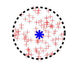
(a) Analytic.

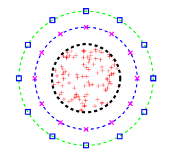
(b) Semi-Analytic.

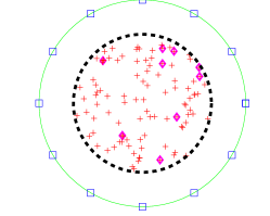
(c) Algebraic.

Fig. 1: We illustrate three methods for computing an outgoing representation of the red source points. In Figure 1(a), we illustrate an analytic, single term expansion: the points are represented by their centroid. Higher order approximations can be viewed as Taylor expansions around this point and require a number of terms that grows significantly with the dimension $d$. In Figure 1(b), we show a method based on placing equivalent sources and finding equivalent densities that can approximate the far field [32]. An outgoing representation is constructed so that the far field due to the true sources (red points) is reproduced by equivalent sources (magenta “X”). The charges on the equivalent sources are determined from interactions with fictitious check points (blue squares). As the dimension of the input increases, the number of equivalent sources and check points required grows quickly, since they must cover the surface of a bounding sphere or cube in $d$ dimensions. In Figure 1(c), we illustrate the skeletonization-based approach. Using the interactions between the sources and fictitious targets (blue squares), the method computes an interpolative decomposition and chooses some skeleton sources (magenta points) to represent the far field. The number of skeleton points needed depends on the local intrinsic dimensionality and the kernel, rather than $d$. However, with existing techniques, the number of targets needed can grow with the ambient dimension.

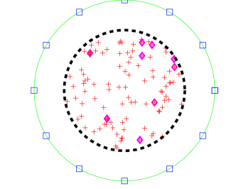
(a) Fictitious targets.

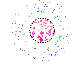
(b) Subsampling (new).

Fig. 2: Two approaches for computing an algebraic outgoing representation. In both cases, we are interested in computing an outgoing representation of the red source points. One method [24] (Figure 2(a)), places a set of fictitious targets covering a ball or box surrounding the sources. It computes the matrix of interactions between targets and sources, and computes its ID. Our approach (Figure 2(b)) subsamples $s$ of the well-separated target points (shown in green). We then compute the ID of the resulting $s\times n$ matrix ${\tilde{K}}$.

Far field using skeletonization. We will use ID to compactly represent the far field of a leaf node $\alpha$. Let ${\mathcal{X}}_{\alpha}$ be the set of points assigned to $\alpha$ (assume ${|{\mathcal{X}}_{\alpha}|}={m}$). Let ${{{K}}_{\alpha}}:=K({{\mathcal{X}}}{\,\setminus\,}{\mathcal{X}}_{\alpha},{\mathcal{X}}_{\alpha})\in\mathbb{R}^{(N-{m})\times{m}}$. Also let $w_{\alpha}=w({\mathcal{X}}_{\alpha})\in\mathbb{R}^{m}$. Our task is to construct an approximation to ${{{K}}_{\alpha}}w_{\alpha}$.

We choose ${s}$, compute the skeleton ${{\mathcal{S}}_{\alpha}}$ of ${{{K}}_{\alpha}}$ and set

(4) $${{{K}}_{\alpha}}w_{\alpha}\approx{\tilde{{{K}}}_{\alpha}}\tilde{w}_{\alpha},\ \mbox{where}\ {\tilde{{{K}}}_{\alpha}}:={{{K}}_{\alpha}}(:,{{\mathcal{S}}_{\alpha}}),\ \tilde{w}_{\alpha}:=w_{\alpha}({{\mathcal{S}}_{\alpha}})+P_{\alpha}w_{\alpha}({\mathcal{R}}),$$

and ${\mathcal{R}}$ is the index set of the unskeletonized columns of ${{{K}}_{\alpha}}$. We term $\tilde{w}_{\alpha}\in\mathbb{R}^{s}$ the skeleton weights.

Given the skeleton ${{\mathcal{S}}_{\alpha}}$ and skeleton weights $\tilde{w}_{\alpha}$, we can efficiently approximate the contribution to some target point ${{u}_{i}}$. We first compute the $1\times s$ matrix of interactions $K({{u}},{{\mathcal{S}}_{\alpha}})$, then apply it to the vector $\tilde{w}_{\alpha}$, to get an approximation with error bounded by (3).

This approach leaves two issues unanswered: first, how do we choose ${s}$? We discuss this in Section 3. Second, computing the ID as described is more expensive than directly evaluating ${{{K}}_{\alpha}}w_{\alpha}$. We address this point next.

Approximate skeletonization. We have $\operatorname{\mathcal{O}}(N/{m})$ leaves and the skeletonization of each leaf described above costs $\operatorname{\mathcal{O}}(N{m}^{2})$. When performed for all leaf nodes, this will require $\operatorname{\mathcal{O}}(N^{2}{m})$ work. Instead, we will compute the skeleton of a smaller matrix, which has only a random subset of the rows of ${{{K}}_{\alpha}}$. That is, we select ${\ell}$ rows with ${m}<{\ell}\ll N$ and whose index set we denote by ${\mathcal{T}}_{\alpha}$. We form ${{{K}}_{\alpha}}({\mathcal{T}}_{\alpha},:)\in\mathbb{R}^{{\ell}\times{m}}$, and compute the skeleton ${{\mathcal{S}}_{\alpha}}$ of size ${s}$ and the corresponding projection matrix $P_{\alpha}$. This is equivalent to choosing ${\ell}$ target points. The complexity of the construction for one leaf becomes $\operatorname{\mathcal{O}}({\ell}{m}^{2})$; thus the overall complexity for all nodes in the tree becomes $\operatorname{\mathcal{O}}(N{\ell}{m})$. This approach is illustrated in Figure 2.

Sampling rows of $K$. We need to choose a small number of rows such that the ID of ${{{K}}_{\alpha}}({\mathcal{T}}_{\alpha},:)$ will be close to the ID of $K$. Randomized linear algebra algorithms can achieve this by either random projections [16] or the construction of an importance sampling distribution [22]. Either approach requires $\operatorname{\mathcal{O}}(N)$ work per node. However, for smoother kernels that decay with distance (or, more generally, dissimilarity) the nearest (more similar) points will tend to dominate the sum in (2). Following this intuition, if we can include the nearest neighbors of each point in ${\mathcal{X}}_{\alpha}$, then we expect this to be a reasonable approximation to an importance sampling distribution. If we do not have enough neighbors, we add additional uniformly chosen points to reach a sufficient sample size. This process is discussed below.

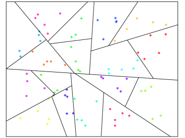
Fig. 3: The tree. An illustration of our median-split binary tree. We split a node by estimating the farthest pair of points in it. We project all points onto the line between these points, then split at the median. The splitting planes are shown, and points belonging to different nodes are shown in different colors.

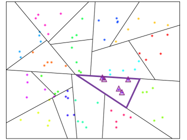
(a) A leaf node.

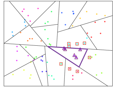
(b) The node’s nearest neighbors.

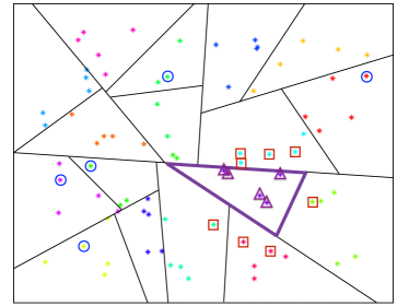
(c) Sampling distant points.

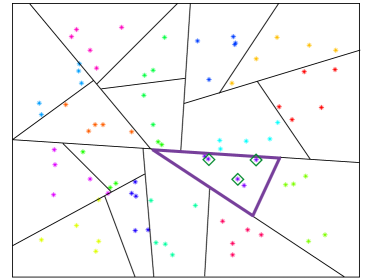
(d) The resulting skeleton.

Fig. 4: Skeletonizing a leaf. Fig. 4(a). We highlight the leaf node to be skeletonized. The points to be approximated are shown with triangles. Fig. 4(b). We compute the union of the lists of nearest neighbors of the points in the leaf, and exclude points that belong to the leaf itself. These points are highlighted with squares. Fig. 4(c). We sample additional distant points for the skeletonization. These points are highlighted with circles. We compute the matrix of interactions with rows given by the neighbors and samples (squares and circles) and columns given by the points in the leaf (triangles). Fig. 4(d). We compute the ID of this matrix to obtain the skeleton points, highlighted with diamonds. Notice that the node has two more points that are not part of the skeleton and will not be used for far-field evaluations. We can now approximate the contribution of the points in this node to a distant target point using only the interactions with these skeleton points.

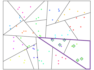
(a) An internal node.

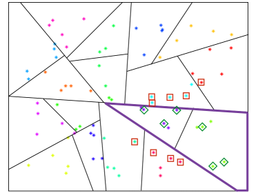
(b) Merging the neighbor lists.

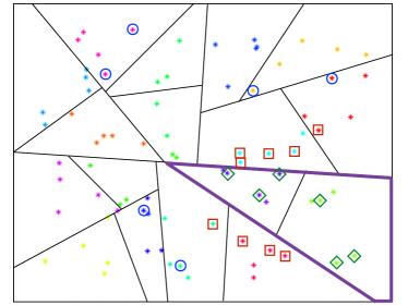
(c) Sampling distant points.

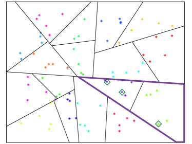
(d) The resulting skeleton.

Fig. 5: Skeletonizing an internal node. Fig. 4(a). We skeletonize the highlighted internal node. The skeletons of its children are highlighted with diamonds. Fig. 4(b). We merge the nearest neighbor lists of the children, then exclude all of the points belonging to the node to be skeletonized. Finding these points can be done in $\operatorname{\mathcal{O}}(\log(N/m))$ time using the Morton IDs. These points are highlighted with squares. Fig. 4(c). We sample additional distant points, highlighted with circles. We compute the matrix of interactions with rows given by the neighbors and samples (squares and circles) and columns given by skeletons of the child nodes (triangles). Fig. 4(d). We compute the ID of this matrix to obtain a skeleton for the parent node, which is a subset of the combined skeletons of the children.

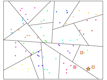
(a) Evaluating at a target point (star).

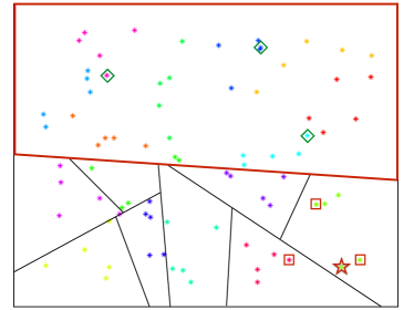
(b) Pruning the highlighted node.

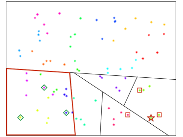
(c) Pruning another node.

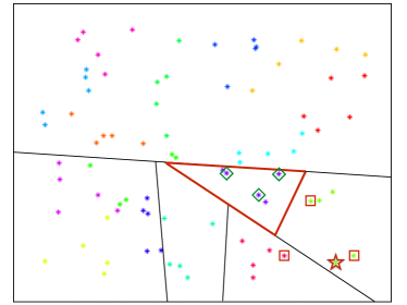
(d) Pruning a leaf node.

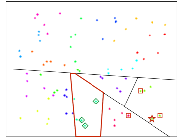
(e) Pruning another leaf node.

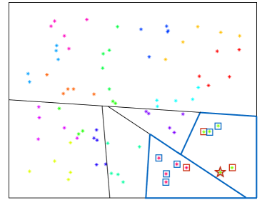
(f) Directly evaluating un-prunable leaves.

Fig. 6: Evaluating the approximate summation. Fig. 6(a). We evaluate the potential at a target point, highlighted with a star. We show its nearest nearest neighbors as well, highlighted with squares. Fig. 6(b). We traverse the tree in a top down fashion. We can prune a node if the node does not contain any neighbors of the target point. By pruning we mean evaluating the field of the node using the skeleton on the target point and then terminating the traversal. The node highlighted in red satisfies our pruning criterion, so we evaluate its contribution approximately. We compute the interactions between the skeleton points (diamonds) and the target. We use the skeleton weights for these points to compute the effective contribution of the node. Fig. 6(c). We continue traversing the tree. Once again, we have a node that contains no nearest neighbors of the target, so we use the skeleton points to compute its approximate contribution. Fig. 6(d). We still use the approximate representation at leaves which satisfy the pruning criterion. Fig. 6(e). We continue the approximate evaluation of all nodes that satisfy the pruning criterion. Fig. 6(f). The leaves highlighted in blue do not satisfy the pruning criterion, so we compute their contribution directly. We evaluate the direct interaction between all points in these nodes (highlighted with squares) and the target point.

2.2 ASKIT

Using the ID as a compact representation, we can now describe the main steps of our treecode:

• Approximate the $\kappa$-nearest neighbors for all ${{x}}_{i}$.

• Compute a top-down binary tree decomposition for ${{\mathcal{X}}}$.

• Perform a bottom-up traversal to build neighbor lists for interior (non-leaf) nodes.

• Perform a bottom-up traversal to compute skeletons and equivalent weights.

• Perform a top-down traversal to evaluate $u_{i}$ at each point $i$.

We describe the individual steps below in detail.

The basic steps of the algorithm are illustrated in Figure 3 (leaves of a tree), Figure 4 (skeletonization of a leaf), 5 (skeletonization of an internal node) and 6 (evaluation).

Computing nearest neighbors. To find nearest neighbors we use a greedy search using random projection trees [7]. We build a tree and for each ${{x}}_{i}$ we collect $\kappa$-nearest neighbors found by exhaustive search among the other points in the leaf node that contains ${{x}}_{i}$. Then we discard the tree (we do not perform top-down searches) and iterate, keeping the best candidate neighbors found at each step. The binary tree used in the treecode is built using the following rule: to split a node $\alpha$, we compute its center (${{x}}_{c}$), then the farthest point to ${{x}}_{c}$ (${{x}}_{l}$), then the farthest point to ${{x}}_{l}$ (${{x}}_{r}$). We project all the points on the line $({{x}}_{l},{{x}}_{r})$, compute the median, and split them into two groups. We recurse until every leaf gets no more than ${m}$ points.

Node neighbor lists. During the skeletonization, we need to sample the far field. To do this we need to construct node neighbor lists. These lists are defined in Algorithm 2 and are constructed in a bottom-up fashion using a standard preorder traversal of the tree.

Algorithm 2 BuildNeighbors($\alpha$)

1:  if IsLeaf$(\alpha)$, ${{\mathcal{N}}_{\alpha}}:=\left({\,\cup\,}_{i\in{\mathcal{X}}_{\alpha}}{{\mathcal{N}}_{i}}\right){\,\setminus\,}{\mathcal{X}}_{\alpha}$

2:  else ${{\mathcal{N}}_{\alpha}}:=\left({{\mathcal{N}}}_{{{\tt r}(\alpha)}}{\,\cup\,}{{\mathcal{N}}}_{{{\tt l}(\alpha)}}\right){\,\setminus\,}\left({{\mathcal{X}}}_{{{\tt r}(\alpha)}}{\,\cup\,}{{\mathcal{X}}}_{{{\tt l}(\alpha)}}\right)$

The set-difference operations can be done in $\operatorname{\mathcal{O}}(\log(N/m))$ time per point using the binary-tree Morton ID of every node and every point. The Morton ID is a bit array that codes the path from the root to the node or point. The Morton ID of a point is the Morton ID of the leaf node which contains it.

Skeletonization of leaves. Let ${\mathcal{X}}_{\alpha}$ be the set of points. Let the contribution of this node to all ${{\mathcal{X}}}{\,\setminus\,}{\mathcal{X}}_{\alpha}$ be denoted as ${{{K}}_{\alpha}}$. As noted above, we will approximate ${{{K}}_{\alpha}}$ by computing a low-rank approximation using an inexact ID that is based on sampling ${{{K}}_{\alpha}}$ to create a matrix ${{K}}({\mathcal{T}}_{\alpha},{\mathcal{X}}_{\alpha})$ for some small set of rows ${\mathcal{T}}_{\alpha}$. Sampling the right points makes a difference and can be expensive. In [23], we developed a sampling scheme that is a hybrid between uniform sampling combined with nearest neighbor sampling (for distance decaying kernels). That is we choose the nearest neighbors of the points in ${\mathcal{X}}_{\alpha}$ which are not themselves in ${\mathcal{X}}_{\alpha}$ and then add uniformly sampled (without replacement) distant points as needed to capture the far field.

(5) $${\mathcal{T}}_{\alpha}={{\mathcal{N}}_{\alpha}}\ {\,\cup\,}\ {\textsc{Sample}}(\ {{\mathcal{X}}}{\,\setminus\,}({\mathcal{X}}_{\alpha}{\,\cup\,}{{\mathcal{N}}_{\alpha}}),\ {\ell}-{|{{\mathcal{N}}_{\alpha}}|}\ ),$$

That is, we randomly sample ${\ell}-{|{{\mathcal{N}}_{\alpha}}|}$ points excluding the points in $\alpha$ and we use these points along with the neighbors ${{\mathcal{N}}_{\alpha}}$ as target points. We then compute the ID of ${{K}}({\mathcal{T}}_{\alpha},{\mathcal{X}}_{\alpha})$ to obtain the skeleton ${{\mathcal{S}}_{\alpha}}$ and skeleton weights $\tilde{w}_{\alpha}$ for ${{{K}}_{\alpha}}$.

On the other hand, if ${|{{\mathcal{N}}_{\alpha}}|}>{\ell}$, we truncate ${{\mathcal{N}}_{\alpha}}$ to only include ${\ell}$ neighbors. We sort the points in ${{\mathcal{N}}_{\alpha}}$ by the distance from their nearest neighbor in $\alpha$, and keep the ${\ell}$ closest points.

Algorithm 3 Skeletonize($\alpha$)

1:  if $\neg$ IsLeaf$(\alpha)$

2:       Skeletonize$({{\tt r}(\alpha)})$, Skeletonize$({{\tt l}(\alpha)})$

3:       ${\mathcal{X}}_{\alpha}={\mathcal{S}}_{{\tt r}(\alpha)}{\,\cup\,}{\mathcal{S}}_{{\tt l}(\alpha)}$

4:  Create sampling targets using (5)

5:  Skeletonize ${\mathcal{X}}_{\alpha}$ using QR factorization and store ${{\mathcal{S}}_{\alpha}}$ and $\tilde{w}_{\alpha}$

Skeletonization of internal nodes. To build the far field approximation for an interior node $\alpha$ we use the same algorithm. Instead of using all the points in the leaf descendants of $\alpha$, we use the combined skeleton points ${\mathcal{S}}_{{{\tt r}(\alpha)}}{\,\cup\,}{\mathcal{S}}_{{{\tt l}(\alpha)}}$ and the neighbors list ${{\mathcal{N}}_{\alpha}}$ constructed with BuildNeighbors$(\alpha)$. Let $\tilde{w}_{{{\tt l}(\alpha)}}$ and $\tilde{w}_{{{\tt r}(\alpha)}}$ be the vectors of skeleton weights of the children.

We compute the ID of the matrix ${{K}}({\mathcal{T}}_{\alpha},{\mathcal{S}}_{{{\tt r}(\alpha)}}{\,\cup\,}{\mathcal{S}}_{{{\tt l}(\alpha)}})$ to obtain a skeleton for $\alpha$ and $P_{\alpha}$. We then apply $P_{\alpha}$ to the unskeletonized part of the concatenation of $\tilde{w}_{{{\tt l}(\alpha)}}$ and $\tilde{w}_{{{\tt r}(\alpha)}}$ to obtain the skeleton weights. These ideas are summarized in SkeletonizeNode$(\alpha)$.

Pruning. During evaluation phase we use a standard top down traversal. For every ${{x}}_{i}$, we start at the root and traverse the tree. The pruning is based on the neighbors of ${{x}}_{i}$ and has nothing to do with distance or kernel evaluations. Node $\alpha$ is not pruned if it is either an ancestor of ${{x}}_{i}$ or it is an ancestor of any of the nearest neighbors of ${{x}}_{i}$:

(6) $${\textsc{Prune}}(\alpha,i)={\textsc{IsTrue}}(\nexists j\in\{i{\,\cup\,}{{\mathcal{N}}_{i}}\}:\alpha\in{\mathcal{A}}_{j})$$

Note that the ancestor check can be done efficiently using Morton IDs. If Prune$(\alpha,i)$ is true, we evaluate the kernel at ${{x}}_{i}$ using the skeleton points and the equivalent weights and do not traverse the children of $\alpha$.

Algorithm 4 $u_{i}=$ Evaluate$({{x}}_{i},\alpha)$

1:  if prune$(\alpha,i)$, return $K({{x}}_{i},{{\mathcal{S}}_{\alpha}}){{\tilde{w}}}_{\alpha}$ {Approximate ((6))}

2:  if IsLeaf$(\alpha)$, return $K({{x}}_{i},{\mathcal{X}}_{\alpha}){{w}}_{\alpha}$ {Direct evaluation}

3:  return ${\textsc{Evaluate}}({{x}}_{i},{{\tt r}(\alpha)})+{\textsc{Evaluate}}({{x}}_{i},{{\tt l}(\alpha)})$ {Recursion}

Algorithm 5 ${u}$=ASKIT$({{\mathcal{X}}},{w},{s},{\ell},{m},{{\mathcal{N}}}({{\mathcal{X}}}))$

1:  $\alpha=$BinaryTree$({{\mathcal{X}}},{m})$ {Build binary tree, $\alpha$ is the root}

2:  BuildNeighbors$(\alpha)$ {Bottom-up traversal}

3:  SkeletonizeNode$(\alpha)$ {Bottom-up traversal}

4:  $u_{i}={\textsc{Evaluate}}({{x}}_{i},\alpha)\quad\forall i\in{{\mathcal{X}}}$ {Top-down traversal}

The evaluation algorithm and the overall scheme are summarized in Algorithm 4 and Algorithm 5 respectively.

To illustrate the difference of the proposed pruning compared to standard distance pruning we conducted a numerical experiment in which we compare the two approaches. The distance pruning criterion is implemented as follows. Given a node $\alpha$ with points ${\mathcal{X}}_{\alpha}$ we compute its centroid $c_{\alpha}$ and a radius $R_{\alpha}=\max_{x\in{\mathcal{X}}_{\alpha}}\|x-c_{\alpha}\|_{2}$. Then given a target point $x$, we prune if $\|x-c_{\alpha}\|_{2}>R$. Notice that in practice $R$ has to be scaled to create some separation between the target and source points, which makes pruning even harder. In Table 2, we report the average number of nodes visited during the tree traversal for evaluating the potential at several target points for a dataset of $N=65,536$ points for different point distributions in 2D, 4D, 32D, and 256D. We used a Gaussian distribution (intrinsic dimension is the same as the ambient dimension), points distributed on a curve (intrinsic dimension is one) and points uniformly distributed on a hypersphere (intrinsic dimension is four). These empirical results show that distance based pruning is not possible in high dimensions even if the underlying intrinsic dimension is small.

dataset	2D		4D		32D		256D
	$R$	$\kappa$	$R$	$\kappa$	$R$	$\kappa$	$R$	$\kappa$
curve	1%	1%	4%	1%	30%	5%	70%	10%
Gaussian	4%	2%	8%	4%	100%	27%	100%	30%
hypersphere	-	-	26%	5%	30%	6%	32%	7%

Table 2: Here we demonstrate the difficulty of distance based pruning in high dimensions. Here dataset indicates the dataset type, which we test in 2, 4, 32, and 256 dimensions. The spiral curve has intrinsic dimensionality one, the hypersphere has intrinsic dimensionality four, and the Gaussian has the same intrinsic dimensionality as the ambient space. The $R$ column indicates distance based pruning and the $\kappa$ column indicates near-neighbor based pruning. The results indicate average values of nodes visited (as a percentage of the total number of nodes in the tree) during the downward pass averaged across target points. We used ${m}=64$ and $\kappa=128$. The larger the number of nodes visited, the less pruning takes place. This results indicate that simple distance based pruning is not effective in high dimensions.

3 Complexity and error

ASKIT has the following parameters that control its computational cost and its accuracy.

• ${m}$: the number of points per leaf node; it controls the error and the runtime since it governs the trade-off between near and far interactions.

• $\kappa$: the number of nearest neighbors for sampling and pruning. The larger $\kappa$ the less we prune. The larger $\kappa$ the better our sample is when we compute the interpolative decomposition. If $\kappa$ is too large the computation becomes quite expensive. In our tests, we set $\kappa=2{m}$ and we have found that increasing $\kappa$ further does not improve the accuracy.

• ${s}$: the skeleton size. In essence, this is the rank we use for the far-field approximation. The higher ${s}$, the more accurate and expensive the skeletonization and evaluation phases are. Here we fixed ${s}$ to be the same in all nodes. A more efficient implementation will be to estimate $\|K_{R}-K_{S}P\|$ and choose ${s}$ adaptively to be different for each node. This is something that we are currently investigating.

• ${\ell}$: the row sampling size for ${{{K}}_{\alpha}}$. Larger values allow a more accurate ID but slower skeletonization. We require ${\ell}>{m}$ and ${\ell}>{s}$ so that ID problem is overdetermined. In our experiments we take ${\ell}={s}+20$. In our experiments taking larger values does not increase the accuracy (if we keep everything else fixed).

So given the choices we describe above, there are two main parameters, the number of points per box ${m}$ and the skeleton size ${s}$.

Computational complexity. We assume that the nearest-neighbor list ${{\mathcal{N}}_{i}}$ for each point is given. Note that exact nearest-neighbors can be computed in $\operatorname{\mathcal{O}}(N)$ time for low-intrinsic dimensional sets [28] and approximation schemes, such as the one we use, are even faster. Thus, we only consider the cost of ASKIT.

The number of leaves is $M=N/{m}$ and the total number of nodes is $2M-1=\operatorname{\mathcal{O}}(M)$. We first consider the upward pass cost or skeletonization cost $T_{S}$. Then we consider the downward evaluation cost $T_{E}$.

In the upward pass, the first calculation is the construction of ${{\mathcal{N}}_{\alpha}}$ the per node neighbor lists that are used for sampling (given by Algorithm 2).

For leaf nodes, the cost of building ${{\mathcal{N}}_{\alpha}}$ (the per-node neighbor lists) involves first merging the per-point neighbor lists $N_{i}$ for all $i\in{\mathcal{X}}_{\alpha}$, sorting them and removing duplicates, and then using the Morton IDs to remove points that belong to a node. The complexity of this operation per node is $\operatorname{\mathcal{O}}(\kappa{m}\log(\kappa{m}))$ and thus the total cost is $\operatorname{\mathcal{O}}(N\kappa\log(\kappa{m}))$. Once we have ${{\mathcal{N}}_{\alpha}}$, we keep only the ${\ell}$ nearest points to the ${\mathcal{X}}_{\alpha}$ and use them to construct the node ID. For internal nodes, the operation is simpler. We simply merge the lists of the children, remove duplicates and points belonging to the node, then sort and truncate to ${\ell}$ points (if necessary). The total complexity is $\operatorname{\mathcal{O}}((N/m){\ell}\log{\ell})$.

The cost of skeletonization involves QR factorizations of $\operatorname{\mathcal{O}}(M)$ matrices of size ${\ell}\times{m}$ (at the leaves) or of size ${\ell}\times(2{s})$ (for internal nodes). In general, the time required for the evaluation of the kernel function depends linearly on $d$. The QR factorization requires $\operatorname{\mathcal{O}}({\ell}{m}^{2})$ for each of the $M$ leaves and $\operatorname{\mathcal{O}}({\ell}{s}^{2})$ time for each of the $\operatorname{\mathcal{O}}(M)$ internal nodes. Thus the total time to construct these matrices and compute their factorizations is $\operatorname{\mathcal{O}}(dM{\ell}({m}^{2}+{s}^{2}))$. Therefore the total time $T_{S}$ for the upward pass (or skeletonization) is given by

(7) $$T_{S}=\operatorname{\mathcal{O}}(N\kappa\log(\kappa{m}))+\operatorname{\mathcal{O}}((N/m)\,{\ell}\log{\ell})+\operatorname{\mathcal{O}}(dN{\ell}({m}^{2}+{s}^{2})/m).$$

The cost of the downward pass depends on our ability to prune. Given a target point $x_{i}$, let $\xi$ be the number of nodes we visit to compute $u_{i}$. We decompose $\xi$ into two parts: $\xi_{n}$ for nodes evaluated directly and $\xi_{f}$ for nodes approximated via the skeleton ($\xi=\xi_{f}+\xi_{n}$). Given these parameters, the cost of the downward pass for point $x_{i}$ is at most $\xi_{n}{m}$ for direct evaluation plus at most $\xi_{f}{s}$ for approximations. Taking the worse case values of $\xi_{n}$ and $\xi_{f}$ for all evaluation points, the overall downward pass cost is bounded by $N(\xi_{n}{m}+\xi_{f}{s})$. We now bound $\xi_{n}$ and $\xi_{f}$.

For $\xi_{n}$, the worst case is that for every point we visit $\kappa$ different leaves, (since we use the point’s nearest neighbors for pruning). Therefore $\xi_{n}\leq\kappa$. Notice that this bound is quite pessimistic since as $m$ increases the will be significant overlap of direct nodes for target points belonging to the same leaf node. Additionally, the number of leaves visited will be smaller in the presence of a low intrinsic dimensional structure. So this estimate is valid only for $m\ll N$.

To bound $\xi_{f}$ we proceed as follows. Given a target point ${{x}}_{i}$, ASKIT will visit all nodes ${\mathcal{A}}({{\mathcal{N}}_{i}})$ and will prune all the remaining nodes. In the worst case, all the elements of ${\mathcal{A}}({{\mathcal{N}}_{i}})$ are unique. Since ${|{{\mathcal{N}}_{i}}|}=\kappa$, ${|{\mathcal{A}}({{\mathcal{N}}_{i}})|}\leq\kappa\log M$. But if these nodes are unique, that means we can prune their siblings by using their skeletonization. Thus, $\xi_{f}=\operatorname{\mathcal{O}}(\kappa\log M)$. That is, we visit $\kappa$ nodes assuming each neighbor of the evaluation belongs to a different leaf node.

Since the cost of evaluating the far field of a node to a point is $\operatorname{\mathcal{O}}(d{s})$ (and assuming $m\ll N$) the overall complexity for $T_{E}$ is given by

(8) $$T_{E}=\operatorname{\mathcal{O}}\left(dN{m}\,\kappa+dN{s}\,\kappa\log\frac{N}{{m}}\right).$$

The total cost of ASKIT it $T=T_{E}+T_{S}$.

Using the fact that in our implementation ${\ell}=\operatorname{\mathcal{O}}({s})$ and $\kappa=\operatorname{\mathcal{O}}({m})$, the overall cost of ASKIT (for $m\ll N$)

(9) $$T=\operatorname{\mathcal{O}}\left(dN{m}\left({s}{m}+\frac{{s}^{3}}{m}+{s}\log\frac{N}{{m}}\right)\right).$$

The ambient dimension $d$ enters only in the cost of kernel evaluations.

Error analysis. There are two sources of error related to ${{{K}}_{\alpha}}$: the far-field low rank approximation and the error in computing this low rank approximation. This error appears in computing the interpolative decomposition factorization due to the selection of a subsample of the rows (the sampling to construct the skeleton). It can be shown that a particular importance sampling distribution (based on what is known as statistical leverage scores) can provide a $\operatorname{\mathcal{O}}(\sigma_{{s}+1})$ reconstruction error if the sample size ${\ell}$ is proportional to ${s}\log{s}$ [22]. However, computing the leverage scores is more expensive than the computation of the kernel summation exactly and thus, cannot be applied in our context.

It is much cheaper to sample using a uniform distribution, but the error bound is not as sharp. In [23], we show that the combined ID approximation and uniform sampling error in the far-field from a single source node to the rest of the points can be bounded as follows. Let $K$ be the $n_{\alpha}\times m_{\alpha}$ matrix of interactions between all the points ${\mathcal{X}}_{\alpha}$ in the source node $\alpha$ and the remaining $n_{\alpha}=N-m_{\alpha}$ points. We sample $\ell$ rows (target points) uniformly and independently and construct a rank $s$ interpolative decomposition of the sampled matrix ${\tilde{K}}$ to select the skeleton size. Then, with high probability, the total error incurred is bounded by

(10) $$\|K-{\tilde{K}}\|\leq\zeta(n_{\alpha},m_{\alpha},{s},\ell)\sigma_{{s}+1}(K).$$

where the quantity $\zeta$ is

(11) $$\zeta(n_{\alpha},m_{\alpha},{s},\ell)=1+\sqrt{6\frac{n_{\alpha}}{\ell}}+\sqrt{1+m_{\alpha}{s}(m_{\alpha}-{s})}.$$

This result is Theorem 3.7 in [23] with $\epsilon=1/2$.

For a given evaluation point, we incur this error each time we prune. We know that the number of prunes is bounded by $\kappa\log\frac{N}{m}$. Denoting by ${\mathcal{V}}_{i}$ the nodes whose skeletonization was used to evaluate the potential at ${{x}}_{i}$, and using the fact that $m_{\alpha}=2^{\mathrm{level}(\alpha)}m$, the overall absolute error is bounded by

(12) $$|u_{i}-u_{\mathrm{exact}}({{x}}_{i})|\leq\|w\|\ \kappa\log\frac{N}{{m}}\ \max_{\alpha\in{\mathcal{V}}_{i}}\ \zeta\left(n_{\alpha},m_{\alpha},{s},\ell\right)\sigma^{\alpha}_{{s}+1}.$$

This is a preliminary result. The remainder of the discussion is qualitative.

We remark that the ambient dimension does not appear in the error estimate; $\kappa$ and errors in finding the exact nearest neighbors affect the maximum of $\sigma^{\alpha}_{{s}+1}$; and the constant $\zeta$ in 11 depends on $n_{\alpha}$, ${s}$, and $\ell$ as well as ${m}_{\alpha}$. This result is derived assuming the skeletonization was computed using uniform random sampling. It is rather pessimistic compared to a result derived for sampling using leverage scores. As we mentioned in our implementation, we employ a heuristic in which we combine nearest neighbors and uniformly chosen samples. We also note that $\sigma_{{s}+1}^{\alpha}$ is bounded by the $({s}+1)^{\textrm{st}}$ singular value of the entire kernel matrix. Therefore, in the case that the entire matrix is low rank, our error bound will be small.

The parameter $\zeta$ can grow significantly if we keep the skeleton size fixed because $\sigma_{{s}+1}^{\alpha}$ can grow and because ${m}_{\alpha}$ grows. To fix this, we can either increase ${s}$ adaptively or we can restrict the $\mathrm{level}(\alpha)$ by starting the evaluation phase at a level which is a fixed distance from the leaves. Also, in lower dimensions, a hybrid pruning rule that combines distances and nearest neighbors could be used to derive sharper error.

How does (12) compare to classical results for treecodes? Using kernel specific analysis and distance pruning one can derive analytic bounds for $\sigma_{{s}+1}$ based on the decay of coefficients in analytic expansions. In that context ${s}$ corresponds to the number of terms in the expansion. There is no explicit dependence of $\zeta$ on $n_{\alpha},{m}_{\alpha}$ since the far field is not computed algebraically or by target sampling. Given that distance pruning is critical in deriving those bounds, it is difficult to relate them to ASKIT since it does not use distance pruning. A critical distance is the distance between the target point ${{x}}_{i}$ and its $(\kappa+1)_{\mathrm{st}}$ nearest neighbor. (Recall that the interactions of $x_{i}$ with all its first $\kappa$ neighbors are computed directly.) The $(\kappa+1)_{\mathrm{st}}$ nearest neighbor may end up being in a node that is pruned. Its distance to ${{x}}_{i}$ resembles the one used in the error estimates using distance pruning and can be used to derive more quantitative bounds. Furthermore it can be used to derive an adaptive (per point) selection of $\kappa_{i}$ to further reduce the overall error of ASKIT.

In summary, equation (12) is suggestive but not particularly useful for quantitatively estimating the error and choosing ${s}$ and $\kappa$. Information regarding the kernel and the point distribution is required to derive a more precise estimate. Next, we present an empirical evaluation of our scheme for the Gaussian kernel with constant and variable bandwidth.

4 Experiments

	parameters			errors			timings (secs)				pruning
run	$\boldsymbol{{m}}$	$\boldsymbol{{s}}$	$\boldsymbol{h}$	hr	$\boldsymbol{\epsilon}$	$\boldsymbol{\epsilon}_{\kappa}$	$\boldsymbol{T}_{\kappa}$	$\boldsymbol{T}$	$\boldsymbol{T}_{S}$	$\boldsymbol{T}_{E}$	near	${\bf far}$
	4D Normal distribution, $N=100,000$,  $T_{\mathrm{direct}}=16$ secs
1	64	4	0.21	97	5E-02	3E-01	5	5	1	4	15%	3 %
2	64	32	0.21	97	1E-02	3E-01	5	7	<1	6	15%	3 %
3	256	128	0.21	87	2E-03	8E-02	7	8	1	7	5 %	1 %
[0.5pt/2pt] 4	64	4	1.00	97	7E-01	1E+00	5	4	<1	4	15%	3 %
5	64	32	1.00	97	6E-02	1E+00	5	7	<1	6	15%	3 %
6	256	128	1.00	88	3E-03	9E-01	7	8	1	7	5 %	1 %
[0.5pt/2pt] 7	64	4	5.00	97	8E-01	1E+00	5	5	<1	4	15%	3 %
8	64	32	5.00	97	1E-04	1E+00	5	7	<1	6	15%	3 %
9	256	128	5.00	88	4E-08	1E+00	7	8	1	7	5 %	1 %
	4D Normal distribution, $N=1,000,000$,  $T_{\mathrm{direct}}=1591$ secs
10	64	4	0.16	95	1E-01	5E-01	56	37	1	36	14%	3 %
11	64	32	0.16	95	3E-02	5E-01	54	71	2	69	14%	3 %
12	256	32	0.16	84	7E-03	3E-01	60	81	3	78	5 %	1 %
	Inexact neighbor information
13	64	4	0.16	26	3E-01	8E-01	31	63	2	61	25%	4 %
14	64	32	0.16	26	5E-02	8E-01	31	119	3	117	25%	4 %
15	64	128	0.16	27	3E-02	8E-01	31	262	4	257	25%	4 %
	16D Normal distribution, $N=1,000,000$,  $T_{\mathrm{direct}}=1630$ secs
16	64	32	0.45	35	1E-03	3E-03	57	573	6	568	83%	23%
17	64	128	0.45	34	7E-04	4E-03	57	725	7	717	83%	23%
18	256	128	0.45	26	1E-04	2E-03	63	997	10	987	55%	8 %
[0.5pt/2pt] 19	64	32	1.76	35	7E-02	1E+00	57	564	6	559	83%	23%
20	64	128	1.76	35	5E-02	1E+00	57	729	7	723	83%	23%
21	256	128	1.76	25	2E-02	1E+00	63	1011	11	1000	55%	8 %
	64D Normal distribution, $N=1,000,000$,  $T_{\mathrm{direct}}=1829$ secs
22	64	128	0.75	8	3E-15	3E-15	63	984	10	974	99%	40%
23	64	128	2.62	8	2E-01	1E+00	63	985	11	975	99%	40%
24	64	128	4.98	8	8E-03	1E+00	63	991	10	981	99%	40%
	4D Normal distribution, variable $h$, $N=1,000,000$,  $T_{\mathrm{direct}}=1622$ secs
25	64	32	1.00	95	3E-02	1E+00	55	145	2	143	14%	3 %
26	64	32	5.00	95	4E-06	1E+00	57	144	2	142	14%	3 %

Table 3: Performance of ASKIT:Here "$\boldsymbol{{m}}$" is points per leaf, "$\boldsymbol{{s}}$" is number of skeleton points, "$\boldsymbol{h}$" the kernel bandwidth, "hr" is the estimated percentage of correct neighbors. The relative error "$\boldsymbol{\epsilon}$" is estimated by direct evaluation on 10K randomly selected points; "$\boldsymbol{\epsilon}_{\kappa}$" is the error if we only use the near field. We report several timings: "$\boldsymbol{T}_{\kappa}$" is the time to construct the nearest neighbor lists, "$\boldsymbol{T}$" is the overall time of ASKIT," $\boldsymbol{T}_{S}$" is skeletonization time, "$\boldsymbol{T}_{E}$" is evaluation time. To illustrate (9), we report the number of tree nodes visited per point during evaluation. "near" is the average number of leaves visited as a percentage of the worst case $\kappa$; "far" the number of nodes whose skeleton was used to evaluate the far field as a percentage of the worst case $\kappa\log(N/{m})$. Also "$\boldsymbol{T}_{\mathrm{dir}}$" is the estimated time for a direct $N^{2}$ evaluation. All times are in seconds. We highlight the error, the treecode time, and the evaluation time. "run" indexes the experiments.

We present results for the Gaussian kernel

$$K({{x}}_{i},{{x}}_{j})=\exp(-\|{{x}}_{i}-{{x}}_{j}\|^{2}_{2}/h_{j}^{2})$$

with constant and variable $h$; we select $h$ based on kernel density estimation theory (Eq. 4.14 in  [29]), so that $h\propto N^{-1/(d+4)}$. The bandwidth $h$ plays a critical role in assessing the accuracy of a treecode. For small and large $h$ the kernel compresses well. But for certain $h$, which depends on the underlying point distribution, the Gaussian kernel does not compress well. The base value we use here is optimal for a constant-width Gaussian kernel and normally distributed points. Also let us remark that doing a simple sweep for $h$ may miss the values of $h$ for which $K$ fails to compress. (More discussion and results can be found in [23].) In our experiments, we choose $h$ large enough so that far-field is necessary for accurate summation and small enough so that the kernel is difficult to compress.

ASKIT has been implemented in C++. The direct evaluation is highly optimized using BLAS but the other parts of the code are proof of principle implementations. We use the Intel MKL for linear algebra, and use OpenMP and MPI parallelism in all phases of the algorithm.

The experiments were carried out on the Stampede system at the Texas Advanced Computing Center. Stampede entered production in January 2013 and is a high-performance Linux cluster consisting of 6,400 compute nodes, each with dual, eight-core processors for a total of 102,400 CPU-cores. The dual-CPUs in each host are Intel Xeon E5 (Sandy Bridge) processors running at 2.7GHz with 2GB/core of memory and a three-level cache. The nodes also feature the new Intel Xeon Phi coprocessors. Stampede has a 56Gb/s FDR Mellanox InfiniBand network connected in a fat tree configuration which carries all high-speed traffic (including both MPI and parallel file-system data).

To test ASKIT, we use normally distributed points in 4, 16, and 64 dimensions for which the intrinsic and ambient dimension coincide. We present results for 100K and 1M points. We also consider the embedding in 1000D of a set of points normally distributed in a 4D hypersphere. We also used a UCI ML repository dataset (SUSY [2]) with 5M points in 18 dimensions. In all experiments, the sources and targets coincide, and we report timings for all pairwise interactions. We present wall-clock times for finding the neighbors, constructing the skeletonization, and the evaluation. Let us remark that for problems that require multiple all-to-all kernel evaluations (e.g., regression), the cost of construction, skeletonization, and neighbor finding is amortized over the iterations. The only per-iteration cost is $T_{E}$.

In Table 3 and Table 4, we report results that show the feasibility of ASKIT. The performance of our nearest neighbor search affects the overall runtimes and the performance of ASKIT. Although it is an independent component, we report the numbers since nearest neighbors must be computed somehow. For this reason, we report the nearest neighbor hit rate accuracy (percentage of correct neighbors) and the timings. We test the accuracy of our nearest-neighbors and ASKIT, using exhaustive searches and direct evaluations on 10K randomly sampled points.

	parameters			errors			timings (secs)				pruning
run	$\boldsymbol{{m}}$	$\boldsymbol{{s}}$	$\boldsymbol{h}$	hr	$\boldsymbol{\epsilon}$	$\boldsymbol{\epsilon}_{\kappa}$	$\boldsymbol{T}_{\kappa}$	$\boldsymbol{T}$	$\boldsymbol{T}_{S}$	$\boldsymbol{T}_{E}$	near	${\bf far}$
	1000D (4d-intrinsic), $N=1,000,000$,  $T_{\mathrm{direct}}=7315$ secs
27	64	32	0.75	99	6E-02	1E+00	204	393	11	382	14%	3 %
28	64	32	3.75	99	2E-06	1E+00	195	391	10	381	14%	3 %
	18D (UCI SUSY), $N=5,000,000$,  $T_{\mathrm{direct}}=41,000$ secs
29	64	128	0.40	91	1E-01	7E-01	709	1510	32	1478	43%	9 %
30	64	128	1.00	90	7E-02	1E+00	567	1530	33	1497	43%	9 %
31	64	128	5.00	90	1E-03	1E+00	577	1566	33	1533	43%	9 %
	MPI-parallel 128D (4d-intrinsic), $N=5,000,000$,  $T_{\mathrm{direct}}=280,000$ secs
32	64	128	0.50	100	1E-03	1E+00	233	1339	12	1158	17%	9%
33	64	128	0.50	100	1E-03	1E+00	43	170	1	144	17%	9%
	MPI-parallel 64D (4d-intrinsic) 512 nodes, (8,192 cores) $N=100,000,000$
34	64	128	0.37	99	1E-02	1E+00	137	1305	6	880	16%	19%

Table 4: Performance of ASKIT: Here "$\boldsymbol{{m}}$" is points per leaf, "$\boldsymbol{{s}}$" is number of skeleton points, "$\boldsymbol{h}$" the kernel bandwidth, "hr" is the estimated percentage of correct neighbors. The relative error "$\boldsymbol{\epsilon}$" is estimated by direct evaluation on 10K randomly selected points; "$\boldsymbol{\epsilon}_{\kappa}$" is the error if we only use the near field. We report several timings: "$\boldsymbol{T}_{\kappa}$" is the time to construct the nearest neighbor lists, "$\boldsymbol{T}$" is the overall time of ASKIT," $\boldsymbol{T}_{S}$" is skeletonization time, "$\boldsymbol{T}_{E}$" is evaluation time. To illustrate (9), we report the number of tree nodes visited per point during evaluation. "near" is the average number of leaves visited as a percentage of the worst case $\kappa$; "far" the number of nodes whose skeleton was used to evaluate the far field as a percentage of the worst case $\kappa\log(N/{m})$. Also "$\boldsymbol{T}_{\mathrm{dir}}$" is the estimated time for a direct $N^{2}$ evaluation. All times are in seconds. We highlight the error, the treecode time, and the evaluation time. "run" indexes the experiments. Runs (33-34) are done using 16 and 256 nodes respectively and the MPI library [15].

Discussion. For low-accuracy approximations our scheme outperforms the direct evaluation at about 1M points. Depending on the kernel and the accuracy the speed-up can be less dramatic or the cutoff may be at much higher $N$. Now we make some additional remarks on our runs.

In runs 1–9 we show how the method converges for different bandwidths and values of ${m}$ and ${s}$ for 100K points that are normally distributed in 4D. Note that the error $\epsilon$ converges with increasing ${m}$ and ${s}$. The convergence can be quite rapid (runs 7–9). In most of the runs, the far-field is critical in getting accuracy. To show this, we report $\epsilon_{\kappa}$, the error in $u$ constructed using only the $\kappa=2{m}$ nearest neighbors for each point. We see that the far field is essential, and truncation does not get a single digit correct. On the other hand for run 22, with $h=0.75$ the far field is wasted effort. In runs 23–24 the far field is essential.

In runs 27-28, we consider a problem in 1000D. The scheme converges quickly and it is 20$\times$ faster than the direct evaluation. For the UCI dataset (29-31) ASKIT is 25$\times$ faster than the direct evaluation. To demonstrate the effects of using the nearest neighbors compare runs 10–12 to runs 13–15. The only difference is that that we use a very approximate search so the hit-rate "hr" (correct neighbors/$\kappa$) small. As a result the errors are higher and the pruning is not as effective (we visit more leaves and more internal nodes). $T_{E}$ is almost 3$\times$ larger. Finally, notice that we increase the dimension the neighbors in general become less accurate. This is because we use a fixed number of iterations in our greedy neighbor search. The skeletonization costs are negligible compared to the evaluation costs.

Runs (1-31) took place on a single node. In runs (32-34) we show a distributed memory run for 5M points in 128D on 16 and 256 nodes resulting a 2000$\times$ speed-up over one-socket direct evaluation. Our largest run on 512 nodes (8,192 cores) we evaluated the sum for 100 million points in 64 dimensions.

5 Conclusions

We presented a new scheme for high dimensional $N$-body problems and conducted a proof-of-concept experimental study. Our scheme is based only on kernel evaluations, uses neighbor-based pruning, and uses neighbor-sampled interpolative decomposition to approximate the far field. Since this method is new, there are many open problems and several opportunities for optimization. The most pressing one is deriving a rigorous error bound that incorporates our sampling scheme; this is ongoing work. There is also further work to be done in optimizing the performance of the scheme, in adaptive determination of the skeleton size, and in improving the sampling. Finally, notice that if we are given similarities and a hierarchical clustering, our scheme does not involve any distance calculations so it should be possible to apply to points (objects) in non-metric spaces.

References

- [1] A. Andoni and P. Indyk, Near-Optimal Hashing Algorithms for Approximate Nearest Neighbor in High Dimensions, Communications of the ACM, 51 (2008), p. 117.
- [2] K. Bache and M. Lichman, UCI machine learning repository, 2013.
- [3] Mario Bebendorf, Approximation of boundary element matrices, Numerische Mathematik, 86 (2000), pp. 565–589.
- [4] Christopher M Bishop, Pattern Recognition and Machine Learning (Information Science and Statistics), Springer-Verlag New York, Inc., 2006.
- [5] Hongwei Cheng, Zydrunas Gimbutas, Per-Gunnar Martinsson, and Vladimir Rokhlin, On the compression of low rank matrices, SIAM Journal on Scientific Computing, 26 (2005), pp. 1389–1404.
- [6] H. Cheng, Leslie Greengard, and Vladimir Rokhlin, A fast adaptive multipole algorithm in three dimensions, Journal of Computational Physics, 155 (1999), pp. 468–498.
- [7] S. Dasgupta and Y. Freund, Random projection trees and low dimensional manifolds, in Proceedings of the 40th annual ACM symposium on Theory of computing, ACM, 2008, pp. 537–546.
- [8] B. Engquist and L. Ying, Fast directional multilevel algorithms for oscillatory kernels, SIAM Journal on Scientific Computing, 29 (2008), pp. 1710–1737.
- [9] William Fong and Eric Darve, The black-box fast multipole method, Journal of Computational Physics, 228 (2009), pp. 8712–8725.
- [10] Zydrunas Gimbutas and Vladimir Rokhlin, A generalized fast mulipole method for nonoscillatory kernels, SIAM Journal on Scientific Computing, 24 (2002), pp. 796–817.
- [11] A.G. Gray and A.W. Moore, N-body problems in statistical learning, Advances in neural information processing systems, (2001), pp. 521–527.
- [12] Leslie Greengard and Vladimir Rokhlin, A fast algorithm for particle simulations, Journal of Computational Physics, 73 (1987), pp. 325–348.
- [13] Leslie Greengard and John Strain, The fast Gauss transform, SIAM Journal on Scientific and Statistical Computing, 12 (1991), pp. 79–94.
- [14] Michael Griebel and Daniel Wissel, Fast approximation of the discrete Gauss transform in higher dimensions, Journal of Scientific Computing, 55 (2013), pp. 149–172.
- [15] W. Gropp, E. Lusk, N. Doss, and A. Skjellum, A high-performance, portable implementation of the MPI message passing interface standard, Parallel Computing, 22 (1996), pp. 789–828.
- [16] N. Halko, P. Martinsson, and J. Tropp, Finding structure with randomness: Probabilistic algorithms for constructing approximate matrix decompositions, SIAM Review, 53 (2011), p. 217.
- [17] Stefan Kurz, Oliver Rain, and Sergej Rjasanow, The adaptive cross-approximation technique for the 3d boundary-element method, Magnetics, IEEE Transactions on, 38 (2002), pp. 421–424.
- [18] Dongryeol Lee, Alexander Gray, and Andrew Moore, Dual-tree fast gauss transforms, Advances in Neural Information Processing Systems, 18 (2006), p. 747.
- [19] Dongryeol Lee and Alexander G Gray, Fast high-dimensional kernel summations using the monte carlo multipole method., in NIPS, 2008, pp. 929–936.
- [20] Dongryeol Lee, Piyush Sao, Richard Vuduc, and Alexander G Gray, A distributed kernel summation framework for general-dimension machine learning, Statistical Analysis and Data Mining, (2013).
- [21] E. Liberty, F. Woolfe, P.G. Martinsson, V. Rokhlin, and M. Tygert, Randomized algorithms for the low-rank approximation of matrices, Proceedings of the National Academy of Sciences, 104 (2007), p. 20167.
- [22] M.W. Mahoney and P. Drineas, Cur matrix decompositions for improved data analysis, Proceedings of the National Academy of Sciences, 106 (2009), p. 697.
- [23] William B. March and George Biros, Far-field compression for fast kernel summation methods in high dimensions, arXiv preprint, (2014), pp. 1–43. www.arxiv.org/abs/1409.2802v1.
- [24] Per-Gunnar Martinsson and Vladimir Rokhlin, An accelerated kernel-independent fast multipole method in one dimension, SIAM Journal on Scientific Computing, 29 (2007), pp. 1160–1178.
- [25] Sebastian Mika, Bernhard Schölkopf, Alex J Smola, Klaus-Robert Müller, Matthias Scholz, and Gunnar Rätsch, Kernel pca and de-noising in feature spaces., in Neural Information Processing Systems, vol. 11, 1998, pp. 536–542.
- [26] Vlad I Morariu, Balaji Vasan Srinivasan, Vikas C Raykar, Ramani Duraiswami, and Larry S Davis, Automatic online tuning for fast Gaussian summation., in NIPS, 2008, pp. 1113–1120.
- [27] Ali Rahimi and Benjamin Recht, Random features for large-scale kernel machines., in NIPS, vol. 3, 2007, p. 5.
- [28] Parikshit Ram, Dongryeol Lee, William March, and Alexander G Gray, Linear-time algorithms for pairwise statistical problems, in Advances in Neural Information Processing Systems, 2009, pp. 1527–1535.
- [29] Bernard W. Silverman, Density Estimation for Statistics and Data Analysis, Chapman and Hall, 1986.
- [30] Johan AK Suykens and Joos Vandewalle, Least squares support vector machine classifiers, Neural processing letters, 9 (1999), pp. 293–300.
- [31] Changjiang Yang, Ramani Duraiswami, Nail A Gumerov, and Larry Davis, Improved fast gauss transform and efficient kernel density estimation, in Computer Vision, 2003. Proceedings. Ninth IEEE International Conference on, IEEE, 2003, pp. 664–671.
- [32] Lexing Ying, George Biros, and Denis Zorin, A kernel-independent adaptive fast multipole method in two and three dimensions, Journal of Computational Physics, 196 (2004), pp. 591–626.
- [33] Kezhong Zhao, Marinos N Vouvakis, and J-F Lee, The adaptive cross approximation algorithm for accelerated method of moments computations of emc problems, Electromagnetic Compatibility, IEEE Transactions on, 47 (2005), pp. 763–773.