Direct $X(3872)$ production in $e^{+}e^{-}$ collisions

Abstract

Direct production of the charmonium-like state $X(3872)$ in $e^{+}e^{-}$ collisions is considered in the framework of the vector meson dominance model. An order-of-magnitude estimate for the width $\Gamma(X\to e^{+}e^{-})$ is found to be $\gtrsim$0.03 eV. The same approach applied to the $\chi_{c1}$ charmonium decay predicts the corresponding width of the order 0.1 eV in agreement with earlier estimates. Experimental perspectives for the direct production of the $1^{++}$ charmonia in $e^{+}e^{-}$ collisions are briefly discussed.

1 Introduction

In 2003 the Belle Collaboration reported the first evidence for the existence of a charmonium-like state $X(3872)$ [1], to be denoted by $X$ for brevity, which possessed properties inconsistent with a plain quark–antiquark meson interpretation. Later this state was confirmed independently by many other experimental collaborations, see Ref. [2] for a recent review article. The quantum numbers of the $X$ were recently determined by the LHCb Collaboration to be $J^{PC}=1^{++}$ [3].

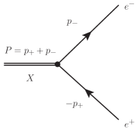
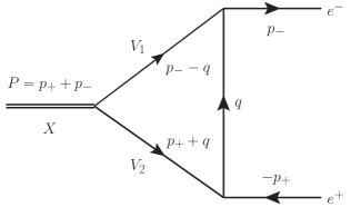
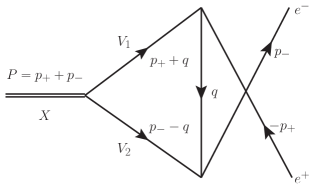
Figure 1: Different contributions to the amplitude for the decay $X\to e^{+}e^{-}$: the first diagram accounts for the short-ranged contributions while the other two describe the transitions $X\to V_{1}V_{2}\to e^{+}e^{-}$ with $\{V_{1},V_{2}\}$ being $\{\rho,J/\psi\}$, $\{\omega,J/\psi\}$, $\{\gamma^{*},J/\psi\}$, and $\{\gamma^{*},\psi^{\prime}\}$.

The aim of the present research is to estimate the production rate of the $X$ directly in $e^{+}e^{-}$ collisions, $e^{+}e^{-}\to X$. This transition is of course forbidden in $e^{+}e^{-}$ annihilation via a single virtual photon, but can occur via two-photon processes of the kind $e^{+}e^{-}\to\gamma^{*}\gamma^{*}\to X$. While in the past such a production of a non-vector state was considered as impossible due to the low production cross section, with the advent of high-luminosity accelerators such as BEPC-II, operating in the charmonium energy region, a detection might become realistic.

Notice that, while the Landau–Yang theorem forbids the coupling of an axial-vector state to two real photons, there is no such ban for the coupling to two virtual photons. To arrive at the desired rate estimate, in this work we parametrise the vertex $X\to\gamma^{*}\gamma^{*}$ in the framework of the vector meson dominance (VMD) model, where either one of the virtual photons or both are replaced by vector mesons (for details we refer to Sec. 3). In addition, for consistency a short-ranged transition amplitude needs to be added. Thus in our model, the decay amplitude is given by the sum of the diagrams depicted in Fig. 1, with the vector pairs $\{V_{1},V_{2}\}$ being $\{\rho,J/\psi\}$, $\{\omega,J/\psi\}$, $\{\gamma^{*},J/\psi\}$, and $\{\gamma^{*},\psi^{\prime}\}$. Decays of the $X$ into all of these four channels were already observed and therefore almost all parameters of the model can be constrained from data. We stress that for this calculation no specific assumptions need to be involved for the nature of the $X$ — the structure information is encoded in the effective coupling constants. To interpret their values in terms of different models is a separate issue that goes beyond the purpose of this work.

2 Useful experimental information

The mass of the $X$ is [4]

$$M_{X}=(3871.68\pm 0.17)~{}\mbox{MeV}.$$ (1)

There exist only upper bounds on its total width [4],

$$\Gamma_{X}<1.2~{}\mbox{MeV},$$ (2)

and on its total production branching fraction in weak $B$-meson decays [5],

$$\mbox{Br}(B\to KX)<3.2\times 10^{-4}.$$ (3)

The quantum numbers of the $X$ were determined to be $J^{PC}=1^{++}$ [3].

The main observation modes for the $X$ are the $D^{0}\bar{D}^{0}\pi^{0}$ [6, 7, 8], $\pi^{+}\pi^{-}J/\psi$ ($\rho J/\psi$) [9, 10, 3] and $\pi^{+}\pi^{-}\pi^{0}J/\psi$ ($\omega J/\psi$) [11], respectively. In addition, radiative decays $X\to\gamma J/\psi$ and $X\to\gamma\psi^{\prime}$ (here and in what follows the shorthand notation $\psi^{\prime}$ is used for the $\psi(2S)$) were also measured. In particular, the BaBar Collaboration reports [12]

$$\mbox{Br}(B^{\pm}\to K^{\pm}X)\mbox{Br}(X\to\gamma J/\psi)=(2.8\pm 0.8\pm 0.2)\times 10^{-6},$$

(4)

$$\mbox{Br}(B^{\pm}\to K^{\pm}X)\mbox{Br}(X\to\gamma\psi^{\prime})=(9.5\pm 2.9\pm 0.6)\times 10^{-6},$$

while the Belle Collaboration gives [13]

$$\mbox{Br}(B^{\pm}\to K^{\pm}X)\mbox{Br}(X\to\gamma J/\psi)=(1.78^{+0.48}_{-0.44}\pm 0.12)\times 10^{-6},$$

(5)

$$\mbox{Br}(B^{\pm}\to K^{\pm}X)\mbox{Br}(X\to\gamma\psi^{\prime})<3.45\times 10^{-6}.$$

The two results are consistent within errors for the $\gamma J/\psi$ mode, however, inconsistent for the $\gamma\psi^{\prime}$ mode. Very recently, the LHCb Collaboration confirmed that the latter mode has a sizable branching fraction [14],

$$R_{\gamma\psi}=\frac{\mbox{Br}(X\to\gamma\psi^{\prime})}{\mbox{Br}(X\to\gamma J/\psi)}=2.46\pm 0.64(\mbox{stat})\pm 0.29(\mbox{syst}).$$ (6)

In order to proceed, we take the averaged value $2.1\times 10^{-6}$ for the product $\mbox{Br}(B^{\pm}\to K^{\pm}X)\mbox{Br}(X\to\gamma J/\psi)$ quoted by the Particle Data Group [4] and then use the inequality (3) and the LHCb ratio (6) to arrive at the following lower bounds

$$\mbox{Br}(X\to\gamma J/\psi)>0.7\,\%,\quad\mbox{Br}(X\to\gamma\psi^{\prime})>1.7\,\%.$$ (7)

Finally, for our estimates we shall use for the width of the $X$

$$\Gamma_{X}=1.0~{}\mbox{MeV},$$ (8)

compatible with the upper bound (2). We also use the following values [4] for the masses:

$$m_{\pi^{0}}=135.0~{}\mbox{MeV},\quad m_{\pi^{\pm}}=139.6~{}\mbox{MeV},\quad m_{\rho}=775.5~{}\mbox{MeV},\quad m_{\omega}=782.7~{}\mbox{MeV},$$

(9)

$$m_{J/\psi}=3096.9~{}\mbox{MeV},\quad m_{\psi^{\prime}}=3686.1~{}\mbox{MeV},\quad M_{X}=3871.7~{}\mbox{MeV},$$

for the total widths:

$$\Gamma_{\rho}=146.2~{}\mbox{MeV},\quad\Gamma_{\omega}=8.5~{}\mbox{MeV},$$ (10)

for the partial leptonic widths:

$$\Gamma(\rho\to e^{+}e^{-})=7.0~{}\mbox{keV},\quad\Gamma(\omega\to e^{+}e^{-})=0.6~{}\mbox{keV},$$

(11)

$$\Gamma(J/\psi\to e^{+}e^{-})=5.6~{}\mbox{keV},\quad\Gamma(\psi^{\prime}\to e^{+}e^{-})=2.4~{}\mbox{keV},$$ (12)

and for the branching fractions:

$$\mbox{Br}(X\to\rho J/\psi)>2.6\,\%,\quad\mbox{Br}(X\to\omega J/\psi)>1.9\,\%.$$ (13)

3 The $X$-vertex

According to the diagrams depicted in Fig. 1, the $X$-vertex that feeds the loops couples an axial-vector state $X$ to two vectors $V_{1}$ and $V_{2}$. Since the $X$ resides very close to the thresholds of the $\rho J/\psi$ and $\omega J/\psi$, the corresponding $X$-vertex can be written in a nonrelativistic form,

$$v_{ijk}(X\to VJ/\psi)=\lambda_{V}\varepsilon_{ijk},\quad V=\rho,\omega,$$ (14)

where $i$, $j$, and $k$ are contracted with the $X$, $V$, and $J/\psi$ polarisation vectors, respectively.

Meanwhile, if one of the vectors is the photon, the nonrelativistic approach does not apply. The relativistic gauge-invariant $X$-vertex takes the form

$$v^{\nu\alpha\beta}(X\to\gamma\psi)=\lambda_{\psi}\varepsilon^{\mu\nu\alpha\beta}k_{\mu},\quad\psi=J/\psi,\psi^{\prime},$$ (15)

with the Lorentz indices $\nu$, $\alpha$, and $\beta$ being contracted with the photon, the $X$, and the $\psi$, respectively, and with $k^{\mu}$ denoting the photon 4-momentum.

The coupling constants $\lambda_{V}$ and $\lambda_{\psi}$ can be related to the corresponding measured partial decay widths of the $X$. In particular, a straightforward calculation gives

$$\Gamma(X\to\gamma\psi)=\Gamma_{X}\mbox{Br}(X\to\gamma\psi)=\frac{\lambda_{\psi}^{2}\omega^{3}}{6\pi M_{X}^{2}},\quad\omega=\frac{M_{X}^{2}-m_{\psi}^{2}}{2M_{X}},$$ (16)

where the experimental branching fractions $\mbox{Br}(X\to\gamma J/\psi)$ and $\mbox{Br}(X\to\gamma\psi^{\prime})$ are quoted in Eq. (7) and the estimate (8) is used for the total $X$ width.

The situation with the $\rho J/\psi$ and $\omega J/\psi$ modes is somewhat more subtle, since what is actually measured are the branching fractions of the processes $X\to\pi^{+}\pi^{-}J/\psi$ and $X\to\pi^{+}\pi^{-}\pi^{0}J/\psi$. We therefore use the vertex (14) to write the amplitude for the process $X\to VJ/\psi\to n\pi J/\psi$ ($n=2,3$) in the form

$$T(X\to n\pi J/\psi)=\lambda_{V}\varepsilon_{ijk}\varepsilon_{i}(X)\varepsilon_{j}(J/\psi)G_{V}(m)v_{k}(V\to n\pi),$$ (17)

where ${\bm{v}}(V\to n\pi)$ is the $V\to n\pi$ vertex, whose explicit form is not needed, and

$$G_{V}(m)=\frac{1}{m^{2}-m_{V}^{2}+im_{V}\Gamma_{V}}.$$

For the width, one has

$$\Gamma(X\to n\pi J/\psi)=\frac{1}{3}\int\sum_{\rm polarisations}{|T(X\to n\pi J/\psi)|^{2}}d\tau,$$ (18)

where for the $X$ at rest as well as for the nonrelativistic $\rho$ or $\omega$ sums over polarisations give 3-dimensional Kronecker deltas. The differential phase space for the final state can be written as

$$d\tau=d\tau_{n\pi}d\tau_{J/\psi}\frac{dm^{2}}{2\pi},\quad d\tau_{J/\psi}=\frac{p(m)}{4\pi^{2}M_{X}},\quad p(m)=\frac{1}{2M_{X}}\lambda^{1/2}(M_{X}^{2},m^{2},m_{J/\psi}^{2}),$$ (19)

with $d\tau_{n\pi}$ being the phase space for the pions, and $\lambda(M^{2},m_{1}^{2},m_{2}^{2})$ is the standard triangle function.

Finally, taking into account that

$$\Gamma(V\to n\pi)=\frac{1}{3}\int\sum_{\rm polarisations}|{\bm{v}}(V\to n\pi)|^{2}d\tau_{n\pi}$$ (20)

and defining a dimensionless integral over the mass distribution of the pions

$$I_{V}\equiv\int_{nm_{\pi}}^{m_{X}-m_{J/\psi}}\Gamma(V\to n\pi)p(m)|G_{V}(m)|^{2}m\,dm,$$ (21)

one arrives at the relation

$$\Gamma(X\to n\pi J/\psi)=\Gamma_{X}\mbox{Br}(X\to n\pi J/\psi)=\frac{\lambda_{V}^{2}I_{V}}{2\pi^{3}M_{X}},$$ (22)

which can be used to extract the couplings $\lambda_{\rho}$ and $\lambda_{\omega}$ with the help of the experimental branching fractions $\mbox{Br}(X\to 2\pi J/\psi)\approx\mbox{Br}(X\to\rho J/\psi)$ and $\mbox{Br}(X\to 3\pi J/\psi)\approx\mbox{Br}(X\to\omega J/\psi)$ quoted in Eq. (13).

In Ref. [15] a theoretical analysis was performed of the experimental mass distributions for the two-pion and three-pion final states reported in Refs. [10, 11]. The results of Ref. [15] allow one to calculate straightforwardly that

$$I_{\rho}\approx 0.2,\quad I_{\omega}\approx 0.02,$$ (23)

where the one order of magnitude difference in the two values comes from the relatively small width of the $\omega$ together with the fact that the nominal $\omega J/\psi$ threshold lies slightly outside of the range of integration in $I_{\omega}$.

The last missing ingredient is the effective vertex $V\to e^{+}e^{-}$ with $V=\rho$, $\omega$, $J/\psi$, and $\psi^{\prime}$, for which we employ the VMD model. The vector meson–photon vertex respecting gauge symmetry can be written as (a detailed discussion of various formulations for the vector mesons can be found in Ref. [16])

$${\cal L}_{V\gamma}=g_{V}(\partial^{\mu}V^{\nu}-\partial^{\nu}V^{\mu})F_{\mu\nu},$$ (24)

where $F_{\mu\nu}$ denotes the usual field strength tensor for the photon. This leads to a photon–vector meson coupling proportional to the photon 4-momentum squared, $k^{2}$. It is this factor that cancels the photon propagator in the transition amplitude $V\to\gamma^{*}\to e^{+}e^{-}$. Therefore the effective $V\to e^{+}e^{-}$ coupling constant is $2eg_{V}$, where $g_{V}$ can be determined from the corresponding leptonic width $\Gamma(V\to e^{+}e^{-})$ quoted in Eq. (11) with the help of the expression

$$\Gamma(V\to e^{+}e^{-})=\frac{4}{3}\alpha g_{V}^{2}m_{V},$$ (25)

derived straightforwardly from the Lagrangian (24).

4 Transition amplitude for $X\to e^{+}e^{-}$

In our VMD approach, the total amplitude of the process $X\to e^{+}e^{-}$ can be written as

$$T(X\to e^{+}e^{-})=\bar{u}(p_{-})V_{\mu}(p_{+},p_{-})u(-p_{+})\varepsilon^{\mu}(X),$$ (26)

where $\varepsilon^{\mu}(X)$ is the $X$ polarisation vector and the full $X$-vertex is given by the sum

$$V_{\mu}(p_{+},p_{-})=v_{\mu}^{\rm reg}+v_{\mu}(X\to\gamma^{*}J/\psi)+v_{\mu}(X\to\gamma^{*}\psi^{\prime}),$$ (27)

with $v_{\mu}^{\rm reg}$ being the regularised contact vertex, and the other two terms are given by the one-loop amplitudes with $\{V_{1},V_{2}\}=\{\gamma^{*},J/\psi\}$, $\{\gamma^{*},\psi^{\prime}\}$. The full transition amplitude is therefore the sum of the diagrams depicted in Fig. 1. Dimensional analysis reveals that the loop integrals in the amplitudes $v_{\mu}(X\to\gamma^{*}J/\psi)$ and $v_{\mu}(X\to\gamma^{*}\psi^{\prime})$ diverge because of the photon momentum entering the $X$-vertex to preserve gauge invariance, see Eq. (15). We employ dimensional regularisation with the $\overline{\rm MS}$ subtraction scheme at the scale $\mu=M_{X}$ and absorb the divergence into the contact vertex $v_{\mu}^{\rm reg}$. In order to provide a prediction for the rate $X\to e^{+}e^{-}$ we need information on the size of this contact term. We here employ two different approaches: on one hand, we vary the scale $\mu$ in a wide range chosen to be from $M_{X}/2$ to $2M_{X}$, which leads to a variation of the divergent integral of the order of its central value. On the other hand, in order to exclude that the contact term is enhanced due to contributions from higher resonances, we explicitly calculate the transition amplitudes $X\to\rho J/\psi\to e^{+}e^{-}$ and $X\to\omega J/\psi\to e^{+}e^{-}$, which contain finite loop integrals only.

5 Transition $X\to VJ/\psi\to e^{+}e^{-}$

For a given vector meson $V$ ($V=\rho,\omega$), the two one-loop contributions to the amplitude $X\to VJ/\psi\to e^{+}e^{-}$ are shown diagrammatically in Fig. 1. The amplitudes read

$$T_{V}^{(1)}=2eg_{V}g_{J/\psi}\lambda_{V}\varepsilon_{i}(X)\varepsilon_{ijk}\int\frac{d^{4}q}{(2\pi)^{4}}\bar{u}(p_{-})\gamma_{j}\not\!{q}\gamma_{k}u(-p_{+})G_{0}(q)G_{V}(p_{-}-q)G_{J/\psi}(p_{+}+q)$$

$$=2eg_{V}g_{J/\psi}\lambda_{V}\varepsilon_{i}(X)\varepsilon_{ijk}\bar{u}(p_{-})\gamma_{j}\gamma_{\mu}\gamma_{k}u(-p_{+})I_{1\mu}(p_{+},p_{-}),$$ (28)

$$T_{V}^{(2)}=2eg_{V}g_{J/\psi}\lambda_{V}\varepsilon_{i}(X)\varepsilon_{ijk}\int\frac{d^{4}q}{(2\pi)^{4}}\bar{u}(p_{-})\gamma_{k}\not\!{q}\gamma_{j}u(-p_{+})G_{0}(q)G_{V}(p_{+}+q)G_{J/\psi}(p_{+}-q)$$

$$=-2eg_{V}g_{J/\psi}\lambda_{V}\varepsilon_{i}(X)\varepsilon_{ijk}\bar{u}(p_{-})\gamma_{j}\gamma_{\mu}\gamma_{k}u(-p_{+})I_{2\mu}(p_{+},p_{-}),$$ (29)

with (the tiny $J/\psi$ width and the electron mass are neglected)

$$G_{0}(p)=\frac{1}{p^{2}+i\epsilon},\quad G_{J/\psi}(p)=\frac{1}{p^{2}-m_{J/\psi}^{2}+i\epsilon},\quad G_{V}(p)=\frac{1}{p^{2}-m_{V}^{2}+im_{V}\Gamma_{V}},$$ (30)

and

$$I_{1\mu}(p_{+},p_{-}) = \frac{1}{i}\int\frac{d^{4}q}{(2\pi)^{4}}q_{\mu}G_{0}(q)G_{V}(p_{-}-q)G_{J/\psi}(p_{+}+q)=\frac{1}{M_{X}^{2}}(A_{V}k_{\mu}+B_{V}P_{\mu}),$$

$$I_{2\mu}(p_{+},p_{-}) = \frac{1}{i}\int\frac{d^{4}q}{(2\pi)^{4}}q_{\mu}G_{0}(q)G_{V}(p_{+}+q)G_{J/\psi}(p_{-}-q)=\frac{1}{M_{X}^{2}}(A_{V}k_{\mu}-B_{V}P_{\mu}),$$

where $P=p_{+}+p_{-}$, $k=p_{+}-p_{-}$ and the relation $I_{2\mu}(p_{+},p_{-})=-I_{1\mu}(p_{-},p_{+})$ was used. Then the full amplitude reads

$$T_{V}=T_{V}^{(1)}+T_{V}^{(2)} = \frac{4B_{V}}{M_{X}^{2}}eg_{V}g_{J/\psi}\lambda_{V}\varepsilon_{i}(X)\varepsilon_{ijk}\bar{u}(p_{-})\gamma_{j}(\not\!{p}_{+}+\not\!{p}_{-})\gamma_{k}u(-p_{+})$$

$$= \frac{16B_{V}}{M_{X}^{2}}eg_{V}g_{J/\psi}\lambda_{V}\varepsilon_{i}(X)\varepsilon_{ijk}p_{k}\bar{u}(p_{-})\gamma_{j}u(-p_{+}),$$

where the Dirac equation with the electron mass neglected, $\bar{u}(p_{-})\not\!{p}_{-}=\not\!{p}_{+}u(-p_{+})=0$, was used. Finally, the width $\Gamma(X\to VJ/\psi\to e^{+}e^{-})$ can be evaluated as

$$\Gamma(X\to VJ/\psi\to e^{+}e^{-})=\frac{16|B_{V}|^{2}}{3\pi M_{X}}\alpha g_{V}^{2}g_{J/\psi}^{2}\lambda_{V}^{2},$$ (32)

where the dimensionless coefficient $B_{V}$ is given by the loop integral,

$$B_{V}=\frac{1}{i}\int\frac{d^{4}q}{(2\pi)^{4}}(qP)G_{0}(q)G_{V}(p_{-}-q)G_{J/\psi}(p_{+}+q)=-\frac{1}{32\pi^{2}}\int_{0}^{1}dx\int_{0}^{1-x}\frac{(x-y)dy}{a_{V}^{2}x+b^{2}y-xy},$$ (33)

with

$$a_{V}^{2}=\frac{m_{V}^{2}-im_{V}\Gamma_{V}}{M_{X}^{2}},\quad b=\frac{m_{J/\psi}^{2}}{M_{X}^{2}}-i\epsilon\ .$$ (34)

We find from a numerical evaluation

$$\Gamma(X\to\rho J/\psi\to e^{+}e^{-})\simeq\Gamma(X\to\omega J/\psi\to e^{+}e^{-})\simeq 10^{-7}~{}\mbox{eV}.$$ (35)

The result of Eq. (35) turns out to be negligible compared to the rate found in the next section. We therefore regard estimating the contribution of the contact term by varying the integration scale over a large range as safe.

6 Transition $X\to\gamma^{*}\psi\to e^{+}e^{-}$

Similarly to the transition amplitude $T_{V}(X\to VJ/\psi\to e^{+}e^{-})$ studied in the previous section, for a given vector meson $\psi$ ($\psi=J/\psi,\psi^{\prime}$), the two contributions to the amplitude $T_{\psi}(X\to\gamma^{*}\psi\to e^{+}e^{-})$ read

$$T_{\psi}^{(1)}=\lambda_{\psi}eg_{\psi}\varepsilon_{\alpha}(X)\varepsilon^{\mu\nu\alpha\beta}\int\frac{d^{4}q}{(2\pi)^{4}}\bar{u}(p_{-})\gamma_{\nu}\not\!{q}\gamma_{\beta}u(-p_{+})(p_{-}-q)_{\mu}G_{0}(q)G_{0}(p_{-}-q)G_{\psi}(p_{+}+q)$$

$$=\lambda_{\psi}eg_{\psi}\varepsilon_{\alpha}(X)\varepsilon^{\mu\nu\alpha\beta}\bar{u}(p_{-})\gamma_{\nu}\gamma_{\lambda}\gamma_{\beta}u(-p_{+})I_{1\mu\lambda}(p_{+},p_{-}),$$ (36)

$$T_{\psi}^{(2)}=\lambda_{\psi}eg_{\psi}\varepsilon_{\alpha}(X)\varepsilon^{\mu\nu\alpha\beta}\int\frac{d^{4}q}{(2\pi)^{4}}\bar{u}(p_{-})\gamma_{\beta}\not\!{q}\gamma_{\nu}u(-p_{+})(p_{+}+q)_{\mu}G_{0}(q)G_{0}(p_{+}+q)G_{\psi}(p_{-}-q)$$

$$=\lambda_{\psi}eg_{\psi}\varepsilon_{\alpha}(X)\varepsilon^{\mu\nu\alpha\beta}\bar{u}(p_{-})\gamma_{\nu}\gamma_{\lambda}\gamma_{\beta}u(-p_{+})I_{2\mu\lambda}(p_{+},p_{-}),$$ (37)

where

$$G_{0}(p)=\frac{1}{p^{2}+i\epsilon},\quad G_{\psi}(p)=\frac{1}{p^{2}-M_{X}^{2}a_{\psi}^{2}+i\epsilon},\quad a_{\psi}^{2}=\frac{m_{\psi}^{2}}{M_{X}^{2}},$$ (38)

and

$$\displaystyle I_{1\mu\lambda}(p_{+},p_{-})=\frac{1}{i}\int\frac{d^{4}q}{(2\pi)^{4}}q_{\lambda}(p_{-}-q)_{\mu}G_{0}(q)G_{0}(p_{-}-q)G_{\psi}(p_{+}+q),$$

$$\displaystyle I_{2\mu\lambda}(p_{+},p_{-})=I_{1\mu\lambda}(p_{-},p_{+}).$$

After some algebra one finds that

$$T_{\psi}=T_{\psi}^{(1)}+T_{\psi}^{(2)}=\lambda_{\psi}eg_{\psi}\varepsilon_{\alpha}\varepsilon^{\mu\nu\alpha\beta}\bar{u}(p_{-})\gamma_{\nu}\left[I_{1}\gamma_{\mu}\gamma_{\beta}+I_{2}\frac{p_{-\mu}p_{+\beta}}{M_{X}^{2}}\right]u(-p_{+}),$$ (39)

where the dimensionless integrals $I_{1}$ and $I_{2}$ are ($D=4-2\varepsilon$)

$$I_{1}=\frac{4i}{D}\int_{0}^{1}dx\int_{0}^{1-x}dy\int\frac{d^{D}q}{(2\pi)^{D}}\frac{q^{2}}{[q^{2}-M_{X}^{2}x(a_{\psi}^{2}-y)]^{3}},$$ (40)

$$I_{2}=8iM_{X}^{2}\int_{0}^{1}xdx\int_{0}^{1-x}(1-2y)dy\int\frac{d^{4}q}{(2\pi)^{4}}\frac{1}{[q^{2}-M_{X}^{2}x(a_{\psi}^{2}-y)]^{3}}.$$ (41)

A straightforward calculation gives:

$$I_{1}^{\rm reg}=\frac{1}{32\pi^{2}}\left[\ln\frac{M_{X}^{2}}{\mu^{2}}-3+a_{\psi}^{2}+\ln a_{\psi}^{2}+(1-a_{\psi}^{2})^{2}\bigg{(}\ln\left(a_{\psi}^{-2}-1\right)-i\pi\bigg{)}\right]$$ (42)

and

$$I_{2}=\frac{1}{4\pi^{2}}(1-a_{\psi}^{2})\left[2+(2a_{\psi}^{2}-1)\left(\ln\left(a_{\psi}^{-2}-1\right)-i\pi\right)\right],$$ (43)

where, as was explained above, the integral $I_{1}$ is calculated using the $\overline{\rm MS}$ scheme. The scale $\mu$ is set equal to $M_{X}$ for the central value and then varied in the range from $M_{X}/2$ to $2M_{X}$ to estimate the uncertainty.

Finally, the width $\Gamma(X\to\gamma^{*}\psi\to e^{+}e^{-})$ takes the form

$$\Gamma(X\to\gamma^{*}\psi\to e^{+}e^{-})=\frac{36\pi\alpha I_{\psi}}{m_{\psi}\left(1-m_{\psi}^{2}/M_{X}^{2}\right)^{3}}\Gamma(X\to\gamma\psi)\Gamma(\psi\to e^{+}e^{-}),$$ (44)

where

$$I_{\psi}=48\left[|I_{1}^{\rm reg}|^{2}+\frac{1}{144}|I_{2}|^{2}+\frac{1}{6}{\rm Re}(I_{1}^{\rm reg}I_{2}^{*})\right],\quad I_{J/\psi}\approx 3.0\times 10^{-3},\quad I_{\psi^{\prime}}\approx 2.4\times 10^{-3}.$$ (45)

Numerical estimates made with the help of Eq. (44) give the following lower bounds:

$$\Gamma(X\to\gamma^{*}J/\psi\to e^{+}e^{-})\gtrsim 10^{-3}~{}\mbox{eV},$$ (46)

$$\Gamma(X\to\gamma^{*}\psi^{\prime}\to e^{+}e^{-})\gtrsim 0.03~{}\mbox{eV}.$$ (47)

Both rates can only be presented as lower bounds, since for the branching fractions given in Eq. (7) only the lower bounds exist. Thus, once better data become available, the results of Eqs. (46) and (47) may be improved. As discussed before, the contribution of the contact term $v_{\mu}^{\rm reg}$ is estimated by varying the scale $\mu$ in a range as wide as from $M_{X}/2$ to $2M_{X}$. This leads to a rather conservative estimate for the intrinsic uncertainty of the rates to be of the order of their central values.

In our approach all parameters are determined from experimental rates. This procedure does not allow us to extract the signs of the couplings and especially the interference pattern between the amplitude with the $\gamma J/\psi$ and the amplitude with the $\gamma\psi^{\prime}$ intermediate state remains undetermined. We therefore use Eq. (47) as the central result and include the possible interference with the $\gamma J/\psi$ intermediate state as a part of the uncertainty.

It should be stressed that in addition to the uncertainties that arise within the formalism used, as discussed above, there is also the uncertainty of the model itself. Unlike effective field theories which have a controlled uncertainty due to a separation of energy scales and the presence of a power counting, our results in Eqs. (46) and (47) should be regarded as an order-of-magnitude estimate, since we are not able to quantify the intrinsic model dependence.

7 Discussion

In this paper we employed a VMD model to estimate the probability of the direct production of the charmonium state $X(3872)$ in $e^{+}e^{-}$ collisions, and we arrived at

$$\Gamma(X\to e^{+}e^{-})\gtrsim 0.03~{}\mbox{eV}$$ (48)

which turned out to be dominated by the $\gamma^{*}\psi^{\prime}$ intermediate state. Within our approach the uncertainty of this value can be estimated to be of the order of 100%. This uncertainty contains the one from our ignorance of a possible short-ranged contribution as well as a possible additional contribution from the $\gamma^{*}J/\psi$ intermediate state. Since it is difficult if not impossible to determine the uncertainty of the model used, we regard the result of Eq. (48) as no more than a proper order-of-magnitude estimate.

To cross-check the approach used, one can apply it to the production of an ordinary charmonium resonance with the same quantum numbers as the $X$, namely the $\chi_{c1}$. Within our approach the process $\chi_{c1}\to e^{+}e^{-}$ proceeds predominantly through the $\gamma^{*}J/\psi$ intermediate state, and its width can be estimated with the help of an equation similar to Eq. (44) with the $X$ replaced by the $\chi_{c1}$. Using the following $\chi_{c1}$ data [4]:

$$m_{\chi_{c1}}=3511~{}\mbox{MeV},\quad\Gamma_{\chi_{c1}}=0.86~{}\mbox{MeV},\quad\mbox{Br}(\chi_{c1}\to\gamma J/\psi)\approx 34.8\%,$$ (49)

our estimate gives 0.1 eV, and appears to be in a qualitative agreement with $\Gamma(\chi_{c1}\to e^{+}e^{-})\simeq 0.46$ eV found in Refs. [17, 18], and higher than the lower bound provided by the unitarity limit: 0.044 eV found in Ref. [17].

Experimentally, a production of the $\chi_{c1}$ state in $e^{+}e^{-}$ collisions seems very promising not only due to the high value of $\Gamma(\chi_{c1}\to e^{+}e^{-})$, but also due to the large branching fraction of $\chi_{c1}$ into $\gamma J/\psi$, which happens to be a clean experimental signature. Especially, if the $J/\psi$ decay into $l^{+}l^{-}$ ($l=e,\mu$) is considered, detailed studies with the BESIII experiment have shown that the only significant background to the $\chi_{c1}$ signal is given by the initial state radiation (ISR) production of $l^{+}l^{-}$ pairs. Neglecting interference effects between the $\chi_{c1}$ and the ISR amplitudes, the signal to background ratio becomes approximately 10% if the value of 0.46 eV is assumed for the electronic width. A discovery of the reaction $e^{+}e^{-}\to\chi_{c1}$ could hence be achieved in an energy scan corresponding to few days of data taking.

It is instructive to consider in addition the ratio

$$\Gamma(X\to e^{+}e^{-}):\Gamma(\chi_{c1}\to e^{+}e^{-})\gtrsim 1:3,$$ (50)

which may cancel some of the uncertainty of the method and thus provides a more reliable prediction. It turns out that the most severe suppression factor in the $X$ production as compared to the $\chi_{c1}$ production comes from the fact that, experimentally, ${\rm Br}(X\to\gamma\psi)\ll{\rm Br}(\chi_{c1}\to\gamma J/\psi)$ (see Eqs. (7) and (49)), while $\Gamma_{X}\approx\Gamma_{\chi_{c1}}$. It should be stressed, however, that the result (50) is based on the upper bound (3) on the total $X$ production in the weak $B$-meson decays, so that decreasing this branching would enhance the width (48) and, accordingly, the ratio (50). Thus we conclude that the probability of the direct $X$ production in $e^{+}e^{-}$ collisions might appear in the same ballpark as the probability of the $\chi_{c1}$ production.

The authors are grateful to Ulf-G. Meißner for careful reading of the manuscript and for valuable comments. This work is supported in part by the DFG and the NSFC through funds provided to the Sino-German CRC 110 “Symmetries and the Emergence of Structure in QCD”, by CRC 1044 “The Low-Energy Frontier of the Standard Model”, by the EU Integrated Infrastructure Initiative HadronPhysics3 (Grant No. 283286), by the Russian presidential programme for the support of the leading scientific schools (Grant No. NSh-3830.2014.2), and by NSFC (Grant No. 11165005).

References

• [1] S.-K. Choi et al., Belle Collaboration, Phys. Rev. Lett. 91 (2003) 262001.
• [2] N.Β Brambilla et al., Eur. Phys. J. C 71 (2011) 1534.
• [3] R. Aaij et al., LHCb Collaboration, Phys. Rev. Lett. 110 (2013) 222001.
• [4] J. Beringer et al., Particle Data Group, Phys. Rev. D 86, (2012) 010001.
• [5] B. Aubert et al, BABAR Collaboration, Phys. Rev. Lett. 96 (2006) 052002.
• [6] G. Gokhroo et al., Belle Collaboration, Phys. Rev. Lett. 97 (2006) 162002.
• [7] B. Aubert et al., BABAR Collaboration, Phys. Rev. D 77 (2008) 011102.
• [8] T. Aushev et al., Belle Collaboration, Phys. Rev. D 81 (2010) 031103.
• [9] A. Abulencia et al., CDF Collaboration, Phys. Rev. Lett. 98 (2007) 132002.
• [10] S.-K. Choi et al., Belle Collaboration, Phys. Rev. D 84 (2011) 052004.
• [11] P. del Amo Sanchez et al., BaBar Collaboration, Phys. Rev. D 82 (2010) 011101(R).
• [12] B. Aubert et al., BaBar Collaboration, Phys. Rev. Lett. 102 (2009) 132001.
• [13] V. Bhardwaj et al., Belle Collaboration, Phys. Rev. Lett. 107 (2011) 091803.
• [14] R. Aaij et al., LHCb Collaboration, arXiv:1404.0275 [hep-ex].
• [15] C. Hanhart, Yu. S. Kalashnikova, A. E. Kudryavtsev, A. V. Nefediev, Phys. Rev. D 85 (2012) 011501(R).
• [16] U.-G.Β Meißner, Phys. Rept. 161 (1988) 213.
• [17] J. H. KΓΌhn, J. Kaplan, and El G. O. Safiani, Nucl. Phys. B 157 (1979) 125.
• [18] J. H. KΓΌhn, talk presented at the International Workshop on $e^{+}e^{-}$ collisions from $\Phi$ to $\Psi$, 9-12 September 2013, Rome, Italy.