Dynamical origin and the pole structure of $X(3872)$

Abstract

The dynamical mechanism of channel coupling with the decay channels is applied to the case of coupled charmonium - $DD^{*}$ states with $J^{PC}=1^{++}$. A pole analysis is done and the $DD^{*}$ production cross section is calculated in qualitative agreement with experiment. The sharp peak at the $D_{0}D^{*}_{0}$ threshold and flat background are shown to be due to Breit-Wigner resonance, shifted by channel coupling from the original position of 3954 MeV for the $2^{3}P_{1}$, $Q\bar{Q}$ state. A similar analysis, applied to the $n=2$, ${}^{3}P_{2}$, $~{}^{1}P_{1}$, ${}^{3}P_{0}$, allows us to associate the first one with the observed $Z(3930)$ $J=2$ and explains the destiny of $~{}^{3}P_{0}$.

The resonance $X(3872)$ found in Choi:2003ue and confirmed and further studied in Acosta:2003zx ; Abazov:2004kp ; Aubert:2004ns ; Barnes:2003vb (see Pakhlova:2008di for review) is still a mysterious phenomenon. The measured quantum numbers of X(3872) Acosta:2003zx suggest that this is a $1^{++}$ state. One can list several properties of this resonance which are difficult to explain. (1) The width of the peak at $3872$ MeV is zero within experimental energy resolution. (2) The peak is exactly at the $D_{0}D_{0}^{*}$ threshold ($3871.2$ MeV) and not at a little higher $D_{+}D_{-}^{*}$ threshold ($3879$ MeV); however, isospin conservation predicts that both thresholds should enter with the same weight. (3) The single-channel theory Eichten_Badalian predicts a standard $2^{\,3}P_{1}$ level of the $Q\bar{Q}$ system around 3950 MeV; however, among the structures observed by Belle in this region, $X(3940),Y(3940),Z(3930)$, there seems to be no examples suggesting the $1^{++}$ identification Pakhlova:2008di . (4) Among the four members of the $2^{3,1}P_{J}$ multiplet, only one with $J=2$ can be associated with $Z(3930)$, which was observed as a regular resonance, $X(3872)$ looks like a sharp cusp, and two others are not seen in this region. It is important to explain this very different behavior.

On the theoretical side there are models based on the $D_{0}D_{0}^{*}$ molecular picture of $X(3872)$ Tornqvist:2004qy_Close:2003sg ; Voloshin:2003nt ; Swanson:2003tb ; Braaten:2005ai and the tetraquark system Maiani_Valcarce_Vijande ; see Godfrey:2009qe for a review. However, one cannot get a simultaneous explanation of points (1)-(4) from these models, and we develop here an alternative approach. It is a purpose of this Letter to exploit a realistic dynamical mechanism, constructed in Danilkin:2009hr , which can explain all four points. Below we shall Briefly explain the mechanism of channel coupling (CC) with the decay channels Danilkin:2009hr . This method allows us to calculate not only position of poles in the CC system, like $Q\bar{Q}$ and $Q\bar{q}$, $\bar{Q}q$, but also scattering amplitudes and production cross sections. We demonstrate that, in the $2^{\,3}P_{1}$ CC system coupled by the $S$-wave decays, two poles originating from complex conjugate Breit-Wigner resonances of $Q\bar{Q}$ system are shifted by CC to the final position, with one pole yielding a narrow cusp at one of thresholds, and another a shifted flat background. We show that when the $CC$ coupling increases, the latter pole yields a very broad bump, and at the same time the weak threshold cusp at the higher threshold $D_{+}D_{-}^{*}$ goes over into a sharp peak at the lower one $D_{0}D_{0}^{*}$. In this way the same value of the coupling constant $\gamma$ (well within the accuracy limits of the universal constant fitted to different charmonium and bottomonium states in Simonov:2007bm ) produces the visible effects, compatible with the properties (1)-(4) mentioned above. To produce this effect as in the $2^{\,3}P_{1}$ state, the original single-channel pole should be above and in the attraction region of the threshold. For the poles originally below threshold, CC shifts poles down, as it happens with the $2^{\,3}P_{2}$ pole. The same approach allows us to explain the situation with two other poles, $2^{\,3}P_{0}$ and $2^{\,1}P_{1}$, as will be discussed below.

Resonances in coupled channels can exist for 3 different reasons Badalian:1981xj : (a) due to bound states in the $Q\bar{Q}$ channel, which are shifted by CC, (b) due to poles in the $(Q\bar{q})(\bar{Q}q)$ channel, shifted by CC; (c) due to strong CC alone (even if no interaction exists in decoupled channel). The most striking feature of the CC resonance is that it approaches the threshold at increasing coupling and typically looks like a pronounced cusp at the threshold of small width. In the realistic physical problem several of these reasons can be present at the same time: e.g., the bare state in the single-channel charmonium can be shifted by strong CC exactly to the threshold. This situation will be discussed below and is characteristic for the single-channel pole above the $S$-wave threshold, where one meets at the same time with the $Q\bar{Q}$, and the strong CC interaction, which shifts the bare charmonium pole exactly to the threshold position and produces a sharp peak. We shall quantitatively describe this situation in the CC formalism of Danilkin:2009hr , where the only changeable parameter is the channel coupling constant $\gamma$ being varied around the standard value.

The basis of the CC theory developed in Danilkin:2009hr ; Simonov:2007bm can be shortly formulated in three relations: a) The effective string decay Lagrangian of the ${}^{3}P_{0}$ type for the decay $Q\bar{Q}\to(Q\bar{q})(\bar{Q}q)$

$$\mathcal{L}_{sd}=\int\bar{\psi}_{q}M_{\omega}\psi_{q}\,d^{4}x$$ (1)

with $M_{\omega}$ tested in charmonium and bottomonium decays Simonov:2007bm , $M_{\omega}\approx 0.8$ GeV where light quark bispinors are treated in the limit of large $m_{c}$ mass as solutions of Dirac equations, and this allows us to go over to the reduced $(2\times 2)$ form of the decay matrix element, $\mathcal{L}_{sd}\to\gamma\int iv_{c}\,\mbox{\boldmath${\rm\sigma}$}\mbox{\boldmath${\rm p}$}\,v\,d^{4}x$, $\gamma=\frac{M_{\omega}}{\langle m_{q}+U-V+\varepsilon_{0}\rangle}\approx 1.4$ (with realistic averages of scalar $U=\sigma r$ and vector $V=-\frac{3}{4}\frac{\alpha_{s}}{r}$ potentials). b) The decay matrix element of the state $n_{1}$ of heavy quarkonium $Q\bar{Q}$ to the states $n_{2}$ and $n_{3}$ of heavy-light mesons $Q\bar{q}$, $\bar{Q}q$,

$$J_{n_{1}n_{2}n_{3}}(\mbox{\boldmath${\rm p}$})= \frac{\gamma}{\sqrt{N_{c}}}\int\frac{d^{\,3}q}{(2\pi)^{3}}\,\bar{y}^{red}_{123}(\mbox{\boldmath${\rm p}$},\mbox{\boldmath${\rm q}$})\,\Psi^{+(n_{1})}_{Q\bar{Q}}(c\mbox{\boldmath${\rm p}$}+\mbox{\boldmath${\rm q}$})$$ (2)

$$\times\,\psi_{Q\bar{q}}^{(n_{2})}(\mbox{\boldmath${\rm q}$})\,\psi^{(n_{3})}_{\bar{Q}q}(\mbox{\boldmath${\rm q}$}).$$

Here all wave functions $(\Psi_{Q\bar{Q}},\,\psi_{Q\bar{q}},\,\psi_{\bar{Q}q})$ refer to the radial parts of the corresponding wave functions, while $\bar{y}^{red}_{123}$ comprises the decay vertex of $\mathcal{L}_{sd}$ and all spin-angular parts of mesons involved; the list of $\bar{y}_{123}^{red}$ for the 6 lowest states is given in Table VII of Danilkin:2009hr . In Eq.2 $c=\frac{\omega_{Q}}{\omega_{q}+\omega_{Q}}$, where the averaged kinetic energies of heavy and light quarks in D meson $\omega_{q}\simeq 0.55$ GeV, $\omega_{Q}\simeq 1.5$ GeV are taken from Badalian:2007km . c) The CC interaction “potential” $V^{CC}_{n_{2}n_{3}}$ between $Q\bar{q}$ and $\bar{Q}q$ mesons due to intermediate states of bound $Q\bar{Q}$ system,

$$V^{CC}_{n_{2}n_{3}}(\mbox{\boldmath${\rm p}$},\mbox{\boldmath${\rm p}$}^{\prime},E)=\sum_{n}\frac{J^{+}_{nn_{2}n_{3}}(\mbox{\boldmath${\rm p}$})J_{nn_{2}n_{3}}(\mbox{\boldmath${\rm p}$}^{\prime})}{E-E_{n}}$$ (3)

and the final $(Q\bar{q})(\bar{Q}q)$ Hamiltonian looks like $H=H_{0}+V^{CC}$, where $H_{0}$ may contain the direct $Q\bar{q}$ and $\bar{Q}q$ interaction, which is $\mathcal{O}(1/N_{c})$ and we disregard it in what follows. The equation for the pole position is Danilkin:2009hr

$$\det[E-\hat{E}-{\hat{w}(E)}]=0,~{}~{}(\hat{E})_{mn}=E_{n}\,\delta_{mn}$$ (4)

where $E_{n}$ is the mass of the bare states and $w_{nm}(E)$ is

$$w_{nm}(E)=\int\frac{d^{\,3}\mbox{\boldmath${\rm p}$}}{(2\pi)^{3}}\sum_{n_{2},n_{3}}\frac{J_{nn_{2}n_{3}}(\mbox{\boldmath${\rm p}$})J^{+}_{mn_{2}n_{3}}(\mbox{\boldmath${\rm p}$})}{E-E_{n_{2}n_{3}}(\mbox{\boldmath${\rm p}$})}\,,$$ (5)

with $E_{n_{2}n_{3}}(\mbox{\boldmath${\rm p}$})=E_{n_{2}}+E_{n_{3}}.$ We shall be interested below in the pole positions, i.e., solutions of (4), and the most important for comparison with experiment, is the production cross section

$$\sigma_{prod}=\sum_{n}\Phi_{n}(E)\frac{\mathrm{Im}\,w_{nn}(E)}{|E-E_{n}-w_{nn}(E)|^{2}},$$ (6)

where $\Phi_{n}(E)$ is a weakly changing function of E. In Figs.2 and Fig.3 this factor is omitted.

We first apply this method to the case of the $1^{++}$ state of $Q\bar{Q}$, and we confine ourselves to one state $2^{3}P_{1}$ in the $Q\bar{Q}$ system so that Eq. (4) reduces to

$$E-E_{n}=w_{nn}(E)$$ (7)

and $w_{nn}$ is given in (5), where $J_{nn_{2}n_{3}}(\mathbf{p})$ should be calculated with the wave functions of $D$ and $D^{*}$ mesons (we disregard here the possible difference in wave functions of $D_{0}$ and $D_{\pm}$, and of $D_{0}^{*}$ and $D_{\pm}^{*}$, and we also disregard all other states $n_{2},n_{3}$ beyond $DD^{*}$). The wave functions of all states involved have been calculated by Badalian et al. Eichten_Badalian , using the relativistic string Hamiltonian Dubin:1994vn derived in the framework of the field correlator method Dosch:1987sk . Here only universal input is used: current quark masses $m_{q}$, string tension $\sigma$ and strong coupling $\alpha_{s}$. These realistic w.f. $(\Psi_{Q\bar{Q}},\,\psi_{Q\bar{q}},\,\psi_{\bar{Q}q})$ have been fitted by a series of oscillator w.f. and in this way both $J_{nn_{2}n_{3}}(\mbox{\boldmath${\rm p}$})$ and $w_{nn}(E)$ were numerically obtained.

To understand the nature of singularities in the energy plane, which produce the cusp at the $D_{0}D_{0}^{*}$ threshold, we find solutions of (7). We separate from $w(E)$ the square root singularity, while the rest is a slowly varying function, which we approximate by $w(E_{th})$

$$w(E)\cong w(E_{th})-\frac{i\tilde{M}}{2\pi}\,k\,|J(0)|^{2}$$ (8)

where $E=E_{th}+k^{2}/2\tilde{M}$ and $\tilde{M}=\frac{M_{D}M_{D^{*}}}{M_{D}+M_{D^{*}}}$ is the reduced mass. Note that $w(E_{th})<0$, and the two pole solutions of Eq.(7) are

$$k_{\pm}=-\frac{ia}{2}\pm\sqrt{-\frac{a^{2}}{4}+b}.$$ (9)

with $a=\tilde{M}^{2}|J(0)|^{2}/\pi$ and $b=2\tilde{M}\,[w(E_{th})+(E_{n}-E_{th})]$. Starting with small coupling, one has two Breit-Wigner poles. With increasing $\gamma$ the square root vanishes at $\gamma=\bar{\gamma}$ and the two poles collide; for $\gamma>\bar{\gamma}$, both poles move apart along imaginary $k$ axis as shown in Fig.1; and at some $\gamma=\gamma^{*},~{}\gamma^{*}=\frac{E_{n}-E_{th}}{|w(E_{th})|},$ the pole $k_{+}$ passes zero, providing the sharp peak at the threshold.

The analysis can be extended to the case of two thresholds $E_{th}^{(1)}$ and $E^{(2)}_{th}$ with the resulting equation

$$\left(k^{2}_{1}-b+ik_{1}\frac{a}{2}\right)^{2}+(k^{2}_{1}-\Delta)\left(\frac{a}{2}\right)^{2}=0,$$

where $\Delta\equiv 2\tilde{M}(E^{(2)}_{th}-E_{th}^{(1)})$. For small $\Delta$ the analysis goes as before, and the only difference in the $k_{1}$ plane is the appearance of the cut connecting points $k_{1}=\pm\sqrt{\Delta}$, which denote access to the second sheet of $k_{2}$. As before, the trajectory of the highest pole $(k^{(+)}_{1})$ passes through the origin, leading to a sharp cusp at $E^{(1)}_{th}$. We have found that the pole never passes through the point $E_{th}^{(2)}$, implying that the peak at $E^{(2)}_{th}$ is never so high, as at $E^{(1)}_{th}$, compare curves (2) and (4) in Fig.2b. These curves correspond to the situations when the pole is closest to $E_{th}^{(2)}$ and when the pole passes the origin, respectively.

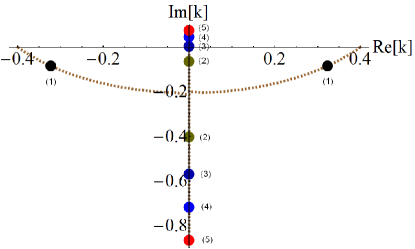
Figure 1: Motion of poles $k_{+}$ (starting on right-hand side) and $k_{-}$ (starting on left-hand side) in the $k$ plane (in units GeV) with growing coupling parameter $\gamma$. Numbers at field circles on curves correspond to numbers on curves in Fig. 2a.

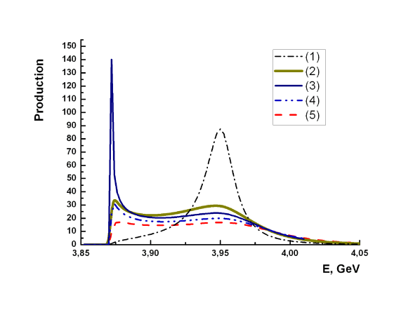
(a) One threshold, $E_{th}(D_{0}D^{*}_{0})$=3.872 GeV.

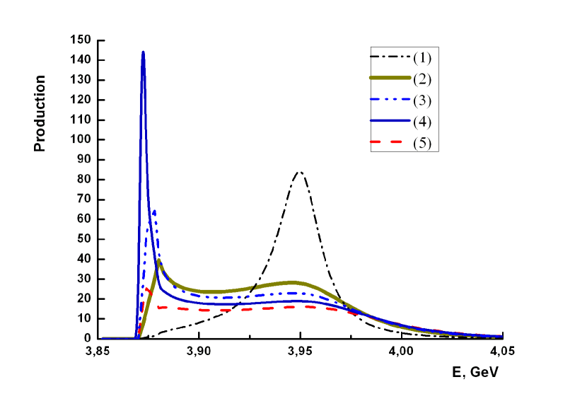
(b) Two thresholds, $E_{th}(D_{0}D^{*}_{0};D_{+}D_{-}^{*})$=3.872; 3.879 GeV.

Figure 2: Production [see Eq. 6] (in units GeV^-1) for $1^{++}$ state with different values of channel coupling parameter [(1) $\gamma=0.6$, (2) $\gamma=1.0$, (3) $\gamma=1.1$, (4) $\gamma=1.2$, (5) $\gamma=1.3$]. For small values of channel coupling parameter $\gamma$ [curve (1)] one can see a good Breit-Wigner shape, which corresponds to the shifted $2^{\,3}P_{1}$ state, while for larger $\gamma$ [curves (3) and (4)] there is a broadening of higher resonance together with steep rise near the threshold $E_{th}(D_{0}D^{*}_{0})=3.872$ GeV.

Summarizing this analysis, we have found the pole structure behind the phenomenon of $X(3872)$, and we may assert that the sharp peak at 3872 is due to the pole $k^{(+)}_{1}$ very close to the $D_{0}D^{*}_{0}$ threshold, which originally was a genuine Breit-Winger pole, and the flat background contains the far virtual pole $k^{(-)}_{1}$, originally the complex conjugated Breit-Wigner pole generated by the same charmonium $2^{3}P_{1}$ state at $\sim 3950$ MeV, and shifted to the final position $k^{(-)}_{1}$ by CC. We stress that the necessary condition for the threshold cusp of the type of $X(3872)$ is $|E_{n}-E_{th}|\approx|w(E_{th})|$, which means that the strength of CC should be as large as the distance of the original $Q\bar{Q}$ bound state from the threshold. In other words, the $Q\bar{Q}$ pole should be “within reach” of CC interaction. One can also see from (9) that for $E_{n}<E_{th}$ the radicand is negative, and for the growing $\gamma$ the pole $k_{+}$ moves up, farther from threshold, so that for moderate $\gamma$ both poles are far from threshold.

In the case of two distinct thresholds $w(E)$ contains two isotopically equivalent thresholds, which we take into account with equal weights. To compare with experiment, we have used the $Q\bar{Q}$ production cross section (6), where $Q\bar{Q}$ (in our case $c\bar{c}$) are produced in some primary reaction, e.g. in $e^{+}e^{-}$ double charmonium production or from $B\to KX$ and then the $Q\bar{Q}\to(Q\bar{q})(\bar{Q}q)$ transition takes place. The resulting form of the cross section is shown in Fig.2b for five different values of $\gamma$. One can see from Fig.2(b) that for weak coupling [curve (1)] only the single-channel charmonium state $E_{n}(2^{3}P_{1})$ is seen with $\Gamma\sim 35$ MeV, and the next two curves display a cusp at $E^{(2)}_{th}$ and an almost disappeared $Q\bar{Q}$ resonance, while curve (4) clearly signals a strong cusp at $E^{(1)}_{th}$ and no other features. At even stronger CC [curve (5)] the CC pole goes away from thresholds and the whole picture flattens. Thus we see that the experimental situation is well reproduced by curve (4). The positions of both poles changing with $\gamma$ are marked in Fig.1. One can easily see how the pole $k_{+}$ produces the sharp cusp in position (3) for one threshold treatment, corresponding to curve (3) in the production cross section in Fig.2(a).

Having found the mechanism, producing the peak at the $D_{0}D_{0}^{*}$ threshold, one may wonder what happens with other states of the $n=2~{}^{3}P_{J}$ family, $J=0,2$. To this end one should first estimate the position of bare poles $E_{n}$ (see Table 1). We use the results of Badalian et al. Eichten_Badalian with the slightly modified spin-orbit interaction.

Table 1: Hadronic shift (MeV) of charmonium $2^{3,1}P_{J}$ bare states $E_{n}$ for different channels. The bare positions were taken from Badalian et al. Eichten_Badalian , $\delta$ is the total shift and $\kappa$ is the closed channel ($D^{*}D^{*}$) suppression coefficient.

State	$J^{PC}$	$E_{n}$	Shifts $(\gamma=1.1)$					$E$	Exp.
			$DD$	$DD^{*}$	$D^{*}D^{*}$		$\delta$
			-	-	$\kappa=0$	0	0	3.969
$2^{3}P_{2}$	$2^{++}$	3969	-	-	$\kappa=0.25$	-14	-14	3.955	Z(3930)
			-	-	$\kappa=0.5$	-27	-27	3.942
$2^{3}P_{1}$	$1^{++}$	3954	to threshold					3.872	X(3872)
			-2	-	$\kappa=0$	0	-2	3.916
$2^{3}P_{0}$	$0^{++}$	3918	-2	-	$\kappa=0.25$	-33	-35	3.883	-
			-2	-	$\kappa=0.5$	-66	-68	3.850
			-	-25	$\kappa=0$	0	-25	3.934
$2^{1}P_{1}$	$1^{+-}$	3959	-	-29	$\kappa=0.25$	-7	-36	3.927	-
			-	-32	$\kappa=0.5$	-14	-46	3.918

We take now the $2^{3}P_{2}$ bare state, which is mostly connected with the $D^{*}D^{*}$ channel, while the $DD$ state is in the $D$ wave and can be neglected. One can see, that $E_{n}(2^{3}P_{2})<E_{th}(D^{*}D^{*})$, and $w(E)$ in (5) is real and negative. Hence, with increasing coupling the pole is shifted down, away from the threshold. This is shown in Table 1. In terms of our previous analysis, using Eq. (9) with $b<0$, one can see that the pole is on the imaginary axis. Moreover, one can estimate that $\sqrt{|b|}\gg\frac{a}{2}$ and the near-the-threshold approximation (8) is not applicable; one can better use the original Eq. (7), which yields a shift of $|w(E_{n})|\sim 55$ MeV. At this point one should take into account the necessity of renormalizing the contributions of higher closed thresholds (which otherwise produce unacceptable shifts, see Kalashnikova:2005ui ; Danilkin:2009hr ; Geiger:1992va ). Therefore we introduce the coefficient $\kappa$, which multiplies in (3) the contribution of the closed channel $D^{*}D^{*}$. We estimate $\kappa$ in an approximate range $0\leq\kappa\leq 0.5$ because it gives the most sensible results for the mass shift of $J/\psi$. However $\kappa$ may depend on quantum state and bare energy. The resulting position is near the experimentally found Pakhlova:2008di $Z(3930)$ peak, as seen in Table 1.

A similar situation occurs for the $2^{3}P_{0}$ state, where the lower threshold is far below, $|E_{n}(2^{3}P_{0})-E_{th}(DD)|\sim 200$ MeV, while the higher threshold is more distant, than in the case of the $2^{3}P_{2}$ state. Our calculation for the shift of the $2^{3}P_{0}$ state yields a large value $\Delta E\sim 68$ MeV for $\kappa=0.5$, see Table 1, so the final position is $3.850$ MeV, which possibly corresponds to the position of the wide peak in $e^{+}e^{-}\to J/\psi D\bar{D}$ in Pakhlov . This enhancement of the shift is due to a much larger overlap matrix element in the ${}^{3}P_{0}$ state. A similar situation was discussed in Kalashnikova:2005ui .

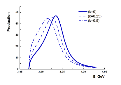
Figure 3: Production (see Eq. 6) [in units GeV^-1] for the $1^{+-}$ state in $DD^{*}$ channel for channel coupling parameter $\gamma=1.1$ and with different values of closed $D^{*}D^{*}$ channel suppression coefficient, $\kappa=0;0.25;0.5$.

An interesting situation occurs in the case of the $1^{+-}$ state with the $2~{}^{1}P_{1}$ pole at bare position 3959 MeV. Here the coupling to the $DD^{*}$ channel is much weaker, than in the case of the $1^{++}$ state, and the main coupling is with the closed $D^{*}D^{*}$ channel, which defines the destiny of the bare pole. When we renormalize the contribution of the $D^{*}D^{*}$ channel with the coefficient $\kappa$, as discussed above, the final shift for $\kappa=0.5$ is around 45 MeV. In Fig. 3 we demonstrate how the production cross section changes with $\kappa$, and one can see, that the resulting width at $\kappa=0.25\div 0.5$ is around $\Gamma\sim 50$ MeV.

In conclusion, we have calculated the amplitudes of CC processes connecting $Q\bar{Q}$ and $(Q\bar{q})(\bar{Q}q)$ systems via the decay matrix element, Eq.(2), involving realistic wave functions of all hadrons involved, and the CC constant $\gamma(M_{\omega})$, fitted earlier to bottomonium and charmonium transitions. For the concrete case of the $1^{++}$ state of charmonium we have found pole structure and production cross section. At small CC two poles correspond to the complex conjugated poles of one Breit-Winger resonance of the $2^{3}P_{1}$ state of $Q\bar{Q}$ with the width $\Gamma\sim 35$ MeV. For increasing CC one of the poles approaches the thresholds and another moves away, as a result this bare resonance flattens, while a sharp cusp appears first at the $D_{+}D_{-}^{*}$ and then at the $D_{0}D_{0}^{*}$ threshold at $\sim 3872$ MeV. This latter situation with the sharp narrow cusp at the $D_{0}D_{0}^{*}$ threshold and absence of any other structures (except for a tiny cusp at higher threshold) including the region around 3940 MeV corresponds to the observed production yield Pakhlova:2008di . We conclude that our dynamical mechanism explains properties (1)-(4), in particular, why the resonance $X(3872)$ is at the lower, but not the higher threshold, why it is so narrow, and why the original $2^{3}P_{1}$ state of charmonium is not seen in experiment.

An alternative and close in spirit approach was developed recently in Kalashnikova:2005ui ; Kalashnikova:2009gt . Our analysis partly supports the conclusion in Zhang:2009bv , that “$X(3872)$ may be of ordinary $c\bar{c}$ $2^{3}P_{1}$ state origin”. Our results differ from those of Ortega:2010qq , where two $1^{++}$ states were found, one associated with $X(3872)$, and another with $X(3940)$. In a recent review Coito:2010cq the CC analysis of the $X(3872)$ and $X(3940)$ was reported with the conclusion, that both states cannot be reproduced in the exploited model simultaneously. This result is in common with ours, since in our case the broad enhancement due to the second pole is near the $D_{0}D_{0}^{*}$ threshold and cannot be associated with $X(3940)$.

The authors are grateful to Yu.S.Kalashnikova for numerous discussions and useful advices, to A.M.Badalian for useful comments, and to M.V.Danilov, G.Pakhlova and P.N.Pakhlov for discussions and suggestions. The financial support of Grant No. 09-02-00629a is gratefully acknowledged.

References

- (1) S. K. Choi et al. [Belle Collaboration], Phys. Rev. Lett. 91, 262001 (2003).
- (2) D. E. Acosta et al. [CDF II Collaboration], Phys. Rev. Lett. 93, 072001 (2004).
- (3) V. M. Abazov et al. [D0 Collaboration], Phys. Rev. Lett. 93, 162002 (2004).
- (4) B. Aubert et al. [BABAR Collaboration], Phys. Rev. D 71, 071103 (2005).
- (5) T. Barnes and S. Godfrey, Phys. Rev. D 69, 054008 (2004).
- (6) G. V. Pakhlova,arXiv:0810.4114 [hep-ex]; G. V. Pakhlova, P. N. Pakhlov, S. I. Eidel’man, Phys. Usp. 53, 219 (2010)
- (7) E. J. Eichten, K. Lane and C. Quigg, Phys. Rev. D 73, 014014 (2006); A. M. Badalian, A. I. Veselov and B. L. G. Bakker, J. Phys. G 31, 417 (2005); A. M. Badalian and I. V. Danilkin, Phys. Atom. Nucl. 72, 1206 (2009); A. M. Badalian, B. L. G. Bakker and I. V. Danilkin, Phys. Atom. Nucl. 72, 638 (2009); A. M. Badalian and B. L. G. Bakker, Phys. Lett. B 646, 29 (2007).
- (8) N. A. Tornqvist, Phys. Lett. B 590, 209 (2004); F. E. Close and P. R. Page, Phys. Lett. B 578, 119 (2004).
- (9) M. B. Voloshin, Phys. Lett. B 579, 316 (2004).
- (10) E. S. Swanson, Phys. Lett. B 588, 189 (2004).
- (11) E. Braaten and M. Kusunoki, Phys. Rev. D 72, 054022 (2005).
- (12) L. Maiani, F. Piccinini, A. D. Polosa and V. Riquer, Phys. Rev. D 71, 014028 (2005); T. Fernandez-Carames, A. Valcarce and J. Vijande, Phys. Rev. Lett. 103, 222001 (2009); J. Vijande, E. Weissman, A. Valcarce and N. Barnea, Phys. Rev. D 76, 094027 (2007); E. Hiyama, H. Suganuma and M. Kamimura, Prog. Theor. Phys. Suppl. 168, 101 (2007).
- (13) S. Godfrey, arXiv:0910.3409 [hep-ph].
- (14) I. V. Danilkin and Yu. A. Simonov, Phys. Rev. D 81, 074027 (2010).
- (15) Yu. A. Simonov, Phys. Atom. Nucl. 71, 1048 (2008); Yu. A. Simonov and A. I. Veselov, Phys. Rev. D 79, 034024 (2009); Phys. Lett. B 671, 55 (2009); JETP Lett. 88, 5 (2008).
- (16) A. M. Badalian, L. P. Kok, M. I. Polikarpov and Yu. A. Simonov, Phys. Rept. 82, 31 (1982).
- (17) A. M. Badalian, B. L. G. Bakker and Yu. A. Simonov, Phys. Rev. D 75, 116001 (2007)
- (18) A. Y. Dubin, A. B. Kaidalov and Yu. A. Simonov, Phys. Lett. B 323, 41 (1994). Phys. Atom. Nucl. 56, 1745 (1993) [Yad. Fiz. 56, 213 (1993)]; A. M. Badalian, A. V. Nefediev and Yu. A. Simonov, Phys. Rev. D 78, 114020 (2008).
- (19) H. G. Dosch, Phys. Lett. B 190, 177 (1987); H. G. Dosch and Yu. A. Simonov, Phys. Lett. B 205, 339 (1988); Yu. A. Simonov, Nucl. Phys. B 307, 512 (1988); A. Di Giacomo, H. G. Dosch, V. I. Shevchenko and Yu. A. Simonov, Phys. Rept. 372, 319 (2002).
- (20) P. Geiger and N. Isgur, Phys. Rev. D 47, 5050 (1993); E. Eichten, K.Lane, C.Quigg, Phys. Rev. D 73, 014014 (2006); M. R. Pennington and D. J. Wilson, Phys. Rev. D 76, 077502 (2007).
- (21) P. N. Pakhlov et al., [Belle Collaboration], Phys. Rev. Lett. 100, 202001 (2008).
- (22) Yu. S. Kalashnikova, Phys. Rev. D 72, 034010 (2005).
- (23) Yu. S. Kalashnikova and A. V. Nefediev, Phys. Rev. D 80, 074004 (2009).
- (24) O. Zhang, C. Meng and H. Q. Zheng, Phys. Lett. B 680, 453 (2009).
- (25) P. G. Ortega, J. Segovia, D. R. Entem and F. Fernandez, Phys. Rev. D 81, 054023 (2010).
- (26) S. Coito, G. Rupp and E. van Beveren, arXiv:1005.2486 [hep-ph].