$Z_{c}(3900)$: what has been really seen?

Abstract

The $Z^{\pm}_{c}(3900)/Z^{\pm}_{c}(3885)$ resonant structure has been experimentally observed in the $Y(4260)\to J/\psi\pi\pi$ and $Y(4260)\to\bar{D}^{\ast}D\pi$ decays. This structure is intriguing since it is a prominent candidate of an exotic hadron. Yet, its nature is unclear so far. In this work, we simultaneously describe the $\bar{D}^{\ast}D$ and $J/\psi\pi$ invariant mass distributions in which the $Z_{c}$ peak is seen using amplitudes with exact unitarity. Two different scenarios are statistically acceptable, where the origin of the $Z_{c}$ state is different. They correspond to using energy dependent or independent $\bar{D}^{*}D$ $S$-wave interaction. In the first one, the $Z_{c}$ peak is due to a resonance with a mass around the $D\bar{D}^{*}$ threshold. In the second one, the $Z_{c}$ peak is produced by a virtual state which must have a hadronic molecular nature. In both cases the two observations, $Z^{\pm}_{c}(3900)$ and $Z^{\pm}_{c}(3885)$, are shown to have the same common origin, and a $\bar{D}^{*}D$ bound state solution is not allowed. Precise measurements of the line shapes around the $D\bar{D}^{*}$ threshold are called for in order to understand the nature of this state.

The resonant-like structure $Z_{c}(3900)^{\pm}$ was first seen simultaneously by the BESIII and Belle collaborations Ablikim:2013mio ; Liu:2013dau in the $J/\psi\pi$ spectrum produced in the $e^{+}e^{-}\to Y(4260)\to J/\psi\pi^{+}\pi^{-}$ reaction. An analysis Xiao:2013iha based on CLEO-c data for the $e^{+}e^{-}\to\psi(4160)\to J/\psi\pi^{+}\pi^{-}$ reaction confirmed the presence of this structure as well, although with a somewhat lower mass. Under a different name, $Z_{c}(3885)^{\pm}$, a similar structure, with quantum numbers favored to be $J^{P}=1^{+}$, has also been reported by the BESIII collaboration Ablikim:2013xfr ; Ablikim:2015swa in the $\bar{D}^{\ast}D$ spectrum of $e^{+}e^{-}\to\bar{D}^{*}D\pi$ at different $e^{+}e^{-}$ center-of-mass (c.m.) energies [including the production of $Y(4260)$]. Because there is a little difference in the central values of the masses and in particular the widths of these two structures, whether they correspond to the same state is still unknown. As will be shown in this Letter, the two structures have indeed the same common origin. We generically denote it here as $Z_{c}$. Evidence for a neutral partner of this structure was first reported in Ref. Xiao:2013iha , and more recently in Ref. Ablikim:2015tbp .

If this resonant structure happens to be a real state as argued in Ref. Guo:2014iya , it is one of the most interesting hadron resonances, since it couples strongly to charmonium and yet it is charged, thus it is something clearly distinct of a conventional $c\bar{c}$ state — its minimal constituent quark content should be four quarks, $c\bar{c}u\bar{d}$ (for $Z_{c}^{+}$). A discussion of possible internal structures is given in Ref. Voloshin:2013dpa . It has been interpreted as a molecular $\bar{D}^{\ast}D$ state Wang:2013cya ; Guo:2013sya ; int:molecules , as a tetraquark of various configurations int:tetraquarks or as a simple kinematical effect int:cusps , although this possibility has been ruled out in Ref. Guo:2014iya . Distinct consequences of some of these different models have been discussed in Ref. Cleven:2015era . It has been also searched for in lattice QCD though with negative results so far int:LQCD .

Being a candidate for an explicitly exotic hadron, the $Z_{c}(3900)$ definitely deserves a detailed and careful study. Indeed, the last years have witnessed an intense theoretical activity aiming at understanding the actual nature of this state. What is still missing, however, is a simultaneous study of the two reactions analysed by BESIII and mentioned above in which the $Z_{c}$ structure has been seen. The goal of this work is to perform such a study, and, from it, to extract information about this seemingly resonant intriguing structure. We will first settle a $\bar{D}^{\ast}D$, $J/\psi\pi$ coupled channel formalism, considering that the $Z_{c}$ emerges from the $\bar{D}^{\ast}D$ interaction, and that its coupling to $J/\psi\pi$ proceeds through the former intermediate state. The resulting $T$-matrix will enter the calculation of the amplitudes for the reactions $Y(4260)\to J/\psi\pi\pi,\bar{D}^{\ast}D\pi$. We will assume that the $Y(4260)$ state is dominantly a $D_{1}(2420)\bar{D}+\text{c.c.}$ bound state Wang:2013cya ; Y4260molecule and use the ideas of Ref. Wang:2013cya to compute the relevant amplitudes.

Let us denote with 1 and 2 the $J/\psi\pi$ and $\bar{D}^{\ast}D$ channels, respectively, with $I=1$ and $J^{PC}=1^{+-}$ (here and below, the $C$-parity refers to the neutral member of the isospin triplet). The coupled-channel $T$-matrix can be written as

$$T=(\mathbb{I}-V\cdot G)^{-1}\cdot V~{},$$ (1)

where $G$ is the loop function diagonal matrix, and the matrix elements of the potential read

$$V_{ij}=4\sqrt{m_{i1}m_{i2}}\sqrt{m_{j1}m_{j2}}\,e^{-q_{i}^{2}/\Lambda_{i}^{2}}e^{-q_{j}^{2}/\Lambda^{2}}C_{ij}~{},$$ (2)

where $m_{i\,n}$ is the mass of the the $n$th particle in the channel $i$, and the mass factors are included to account for the non-relativistic normalization of the heavy meson fields. The $J/\psi\pi\to J/\psi\pi$ interaction strength is known to be tiny Yokokawa:2006td ; Liu:2012dv , and we neglect the direct coupling of this channel, $C_{11}=0$. Such a treatment was also done in Ref. Hanhart:2015cua in a coupled-channel analysis of the $Z_{b}$ states. For the inelastic $\bar{D}^{\ast}D\to J/\psi\pi$ $S$-wave interaction, we make the simplest possible assumption, that amounts to take it to be a constant, $C_{12}\equiv\widetilde{C}$. In a momentum expansion, the lowest order contact potential for the $\bar{D}^{\ast}D\to\bar{D}^{\ast}D$ transition is simply a constant as well, denoted by $C_{22}\equiv C_{1Z}$ HQSSFormalism . However, it can be shown that even with two coupled channels, no resonance can be generated in the complex plane above threshold with only constant potentials. To that end, we will also allow some energy dependence for the $V_{22}$ term, introducing a new parameter $b$, and writing

$$C_{22}(E)=C_{1Z}+b\left(E-m_{D}-m_{D^{\ast}}\right)$$ (3)

with $E$ the total c.m. energy. The new term is of higher order in low-momentum expansion in comparison with $C_{1Z}$. The interactions considered here need to be regularized in some way, and hence we employ a standard gaussian regulator Epelbaum:2008ga , $e^{-q_{i}^{2}/\Lambda_{i}^{2}}$, where the c.m. momentum squared of the channel $i$ is denoted by ${q_{i}}^{2}$. We adopt a relativistic (non-relativistic) definition of the latter for the $i=1$ ($i=2$) channel, i.e., ${q_{1}}^{2}=\lambda(E^{2},m_{J/\psi}^{2},m_{\pi}^{2})/(4E^{2})$ and ${q_{2}}^{2}=2\mu(E-m_{D}-m_{D^{\ast}})$, being $\mu$ the reduced mass of the $\bar{D}^{\ast}D$ system. Since the interaction for this channel is derived from a non-relativistic field theory, we take cutoff values $\Lambda_{2}=0.5-1\ \text{GeV}$ HQSSFormalism . At the $Z_{c}$ energy, the c.m. momentum of the $J/\psi\pi$ channel is $q_{1}\simeq 0.7\ \text{GeV}$, and hence we use a different cutoff for it. For definiteness, we set $\Lambda_{1}=1.5\ \text{GeV}$, although the specific value is not very relevant as we have checked since changes in the cut-off can be reabsorbed in the strength of the transition potential controlled by the undertermined $C_{12}$ low energy constant. With this convention for the regulator, the loop functions in the matrix $G$ read

$$G_{1}(E) =\int\frac{l^{2}dl}{4\pi^{2}}\frac{\omega_{1}+\omega_{2}}{\omega_{1}\omega_{2}}\frac{e^{-(l^{2}-q_{1}^{2})/\Lambda_{1}^{2}}}{E^{2}-(\omega_{1}+\omega_{2})^{2}+i\epsilon}~{},$$ (4)

$$G_{2}(E) =\frac{1}{m_{D}+m_{D^{\ast}}}\int\frac{l^{2}dl}{4\pi^{2}}\frac{e^{-(l^{2}-q_{2}^{2})/\Lambda_{2}^{2}}}{q_{2}^{2}-l^{2}+i\epsilon}~{},$$ (5)

with $\omega_{n}=\sqrt{l^{2}+m_{1n}^{2}}$. The $D\bar{D}^{\ast}$ channel loop function $G_{2}$ is computed in the non-relativistic approximation.

For the $e^{+}e^{-}$ annihilations at the $Y(4260)$ mass, both BESIII and Belle have reported the $Z_{c}$ structure in the $J/\psi\pi$ final state Ablikim:2013mio ; Liu:2013dau , but only BESIII provides data for the $\bar{D}^{\ast}D$ channel Ablikim:2013xfr ; Ablikim:2015swa . Hence, for consistency, we will only study the BESIII data. In particular, we will consider the most recent double-$D$-tag data of Ref. Ablikim:2015swa , in which the $D^{\ast}$ is reconstructed from several decay modes, whereas in Ref. Ablikim:2013xfr the presence of the $D^{\ast}$ is only inferred from energy conservation. Hence, in the former data the background in the higher energy $D^{\ast}D$ invariant mass regions is much reduced. For definiteness, we will consider the reported spectra of the $D^{\ast-}D^{0}$ and $J/\psi\pi^{-}$ final states, and set $m_{D^{\ast}}=m_{D^{\ast-}}$, $m_{D}=m_{D^{0}}$, and $m_{\pi}=m_{\pi^{\pm}}$. This implicitly assumes that isospin breaking effects are neglected. These data are taken at a c.m. energy equal to the nominal $Y(4260)$ mass, so the decays to $\pi(J/\psi\pi,\bar{D}^{\ast}D)$ proceed mainly through the formation of this resonance. The mechanisms for the $Y(4260)$ decays are shown in Fig. 1. The coupling $YD_{1}D$, whose value is not important here to describe the lines shapes, is taken from Ref. Wang:2013cya , where the $Y(4260)$ is considered to be dominantly a $\bar{D}D_{1}+\text{c.c.}$ bound state. The subsequent $D_{1}D^{\ast}\pi$ coupling can also be found there.

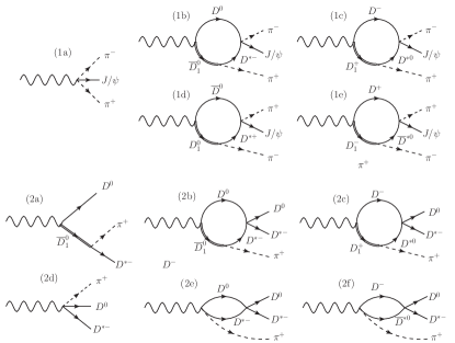
Figure 1: Diagrams contributing to the $Y(4260)$ (wavy line) decays to $\bar{D}^{\ast}D\pi$ and $J/\psi\pi\pi$.

We denote $\mathcal{M}_{1}$ ($\mathcal{M}_{2}$) to the amplitude for the $Y\to J/\psi\pi^{+}\pi^{-}$ ($Y\to D^{\ast-}D^{0}\pi^{+}$) decay, and $s$ and $t$, respectively, to the invariant masses squared of $J/\psi\pi^{-}$ and $J/\psi\pi^{+}$ ($D^{\ast-}D^{0}$ and $D^{\ast-}\pi^{+}$) in the first (second) decay. Up to some common irrelevant constant, both amplitudes can be written (after the appropriate sum and average over polarizations) as:

$$\left\lvert\overline{\mathcal{M}_{1}}(s,t)\right\rvert^{2}=\left\lvert\tau(s)\right\rvert^{2}q^{4}_{\pi}(s)+\left\lvert\tau(t)\right\rvert^{2}q^{4}_{\pi}(t)$$

$$+\frac{3\cos^{2}\theta-1}{4}\big{(}\tau(s)\tau(t)^{\ast}+\tau(s)^{\ast}\tau(t)\big{)}q^{2}_{\pi}(s)q^{2}_{\pi}(t)~{},$$ (6)

$$\tau(s)=\sqrt{2}I_{3}(s)T_{12}(s)+\alpha~{},$$ (7)

$$\left\lvert\overline{\mathcal{M}_{2}}(s,t)\right\rvert^{2}=\left\lvert\frac{1}{t-m_{D_{1}}^{2}}+I_{3}(s)T_{22}(s)\right\rvert^{2}q^{4}_{\pi}(s)$$

$$+\left\lvert\beta\big{(}1+T_{22}(s)G_{2}(s)\big{)}\right\rvert^{2}~{},$$ (8)

where $q^{2}_{\pi}(s)=\lambda(M_{Y}^{2},s,m_{\pi}^{2})/(4M_{Y}^{2})$, and $\theta$ denotes the relative angle between the two pions in the $Y(4260)$ rest frame. Further, $I_{3}(s)$ is the scalar three-meson non-relativistic loop function, for which details can be found in Ref. Albaladejo:2015dsa . One first notes that $\overline{\mathcal{M}_{1}}(s,t)$ is symmetric under $s\leftrightarrow t$. The term with $\alpha$ represents diagram (1a), and it acts as a non-resonant background amplitude, added coherently to the rest of the diagrams. It has the same dependence on the external momenta and polarization vectors as that of diagrams (1b)–(1e). The first term in $\overline{\mathcal{M}_{1}}(s,t)$ is the amplitude of diagrams (1b)+(1c), the second term is the one from diagrams (1d)+(1e), and the last one is their interference. In $\overline{\mathcal{M}_{2}}$, the first summand of the first term corresponds to diagram (2a) in Fig. 1, whereas the second one, which includes the $\bar{D}^{\ast}D$ final state interaction (FSI), is the contribution from diagrams (2b)+(2c). Diagrams (2a)-(2c) proceed through the formation of $D_{1}$, but we also consider some non-resonant $\bar{D}^{\ast}D\pi$ production by means of diagram (2d). The $\bar{D}^{\ast}D$ rescattering effects in this last diagram give rise, in turn, to diagrams (2e) and (2f). The term with $\beta$ in Eq. (8) represents these latter three diagrams. The parameters $\alpha$ and $\beta$ in Eqs. (7) and (8) are unknown. Note that the effect of $D_{1}$ width, $\Gamma_{D_{1}}=(25\pm 6)$ MeV, is negligible here since $m_{D_{1}}+m_{D}-\Gamma_{D_{1}}/2$ is well above 4.26 GeV.

The spectrum for both reactions can be obtained as a contribution from the amplitudes ($\mathcal{A}_{i}$) plus a background ($\mathcal{B}_{i}$):

$$\mathcal{N}_{i}(s) =K_{i}\left(\mathcal{A}_{i}(s)+\mathcal{B}_{i}(s)\right)~{},$$ (9)

$$\mathcal{A}_{i}(s) =\int_{t_{i,-}}^{t_{i,+}}\!\!\!\!dt\left\lvert\overline{\mathcal{M}_{i}}(s,t)\right\rvert^{2}~{},$$ (10)

where $t_{i,\pm}(s)$ are the limits of the $t$ Mandelstam variables for the decay mode $i$. The two global constants $K_{i}$ could be related if the event selection efficiencies of the two spectra analyzed in this work were known. If the latter were roughly the same, then one would have $K_{1}\simeq 5K_{2}$ (due to the different bin sizes). If both parameters are considered free, a large correlation arises between $K_{1}$ and $\widetilde{C}$, since $K_{1}\lvert\widetilde{C}\rvert^{2}$ basically determines the total strength of the event distribution $\mathcal{N}_{1}$. This is due to the fact that the influence of $\widetilde{C}$ in the shape of the $T$-matrix elements, and thus of the signal of $Z_{c}$ in the spectrum, is small. To obtain a reasonable estimate of this coupling constant, we consider a further experimental input from Ref. Ablikim:2013xfr ,

$$R_{\text{exp}}=\frac{\Gamma\left(Z_{c}(3885)\to D\bar{D}^{\ast}\right)}{\Gamma\left(Z_{c}(3900)\to J/\psi\pi\right)}=6.2\pm 1.1\pm 2.7~{},$$ (11)

and estimate this ratio as

$$R_{\text{th}}=\frac{\int ds\mathcal{A}_{2}(s)}{\int ds\mathcal{A}_{1}(s)}~{},$$ (12)

that is, as the ratio of the background subtracted areas of each physical spectrum around the $Z_{c}$ mass, namely in the range $\sqrt{s}=(3900\pm 35)\ \text{MeV}$.

In principle, the double-$D$-tag technique ensures that all the $\bar{D}^{\ast}D$ spectrum events in Ref. Ablikim:2015swa contain a $\bar{D}^{\ast}D$ pair, so there is no background due to wrong identification of the final state. There could be, however, contributions to the spectrum from higher waves other than the $S$-wave. In any case, an inspection of Fig. 2 shows that the tail of the spectrum is small, and we set $\mathcal{B}_{2}=0$. We shall come to this point later on. For the $J/\psi\pi$ spectrum, $\mathcal{B}_{1}$ is parameterized with a symmetric smooth threshold function as used in the experimental work of Ref. Ablikim:2013mio :

$$\mathcal{B}_{1}(s)=B_{1}\left[(\sqrt{s}-m_{1-})(m_{+}-\sqrt{s})\right]^{d_{1}}~{},$$ (13)

with $m_{1-}=m_{J/\psi}+m_{\pi}$ and $m_{+}=m_{Y}-m_{\pi}$, i.e., the limits of the available phase space for the reaction. The parameters $B_{1}$ and $d_{1}$ are free.

$\Lambda_{2}\ (\text{GeV})$	$C_{1Z}\ (\text{fm}^{2})$	$b\ (\text{fm}^{3})$	$\widetilde{C}\ (\text{fm}^{2})$	$\chi^{2}/\text{dof}$	$R_{\text{th}}$
$1.0$	$-0.19\pm 0.08\pm 0.01$	$-2.0\pm 0.7\pm 0.4$	$0.39\pm 0.10\pm 0.02$	$1.02$	$\hphantom{1}6.0\pm 3.5\pm 0.5$
$0.5$	$\hphantom{+}0.01\pm 0.21\pm 0.03$	$-7.0\pm 0.4\pm 1.4$	$0.64\pm 0.16\pm 0.02$	$1.09$	$\hphantom{1}6.5\pm 3.6\pm 0.2$
$1.0$	$-0.27\pm 0.08\pm 0.07$	$0$ (fixed)	$0.34\pm 0.14\pm 0.01$	$1.31$	$10.3\pm 9.0\pm 1.1$
$0.5$	$-0.27\pm 0.16\pm 0.13$	$0$ (fixed)	$0.54\pm 0.16\pm 0.02$	$1.36$	$10.9\pm 9.0\pm 2.5$

Table 1: Parameters of the $T$-matrix obtained for the different fits performed in this work, together with the reduced $\chi^{2}$ and the ratio $R_{\text{th}}$ obtained. The first (second) error is statistical (systematic). The pole position found for the $Z_{c}$ state in each case is given, in the same order as here, in Table 2.

$M_{Z_{c}}$ (MeV)	$\Gamma_{Z_{c}}/2$ (MeV)	Ref.	Final state
$3899\pm 6$	$23\pm 11$	Ablikim:2013mio (BESIII)	$J/\psi\ \pi$
$3895\pm 8$	$32\pm 18$	Liu:2013dau (Belle)	$J/\psi\ \pi$
$3886\pm 5$	$19\pm\hphantom{1}5$	Xiao:2013iha (CLEO-c)	$J/\psi\ \pi$
$3884\pm 5$	$12\pm\hphantom{1}6$	Ablikim:2013xfr (BESIII)	$\bar{D}^{\ast}D$
$3882\pm 3$	$13\pm\hphantom{1}5$	Ablikim:2015swa (BESIII)	$\bar{D}^{\ast}D$
$3894\pm 6\pm 1$	$30\pm 12\pm 6$	$\Lambda=1.0$ GeV	$J/\psi\ \pi$, $\bar{D}^{\ast}D$
$3886\pm 4\pm 1$	$22\pm\hphantom{1}6\pm 4$	$\Lambda=0.5$ GeV	$J/\psi\ \pi$, $\bar{D}^{\ast}D$
$3831\pm 26^{+\hphantom{1}7}_{-28}$	virtual state	$\Lambda=1.0$ GeV	$J/\psi\ \pi$, $\bar{D}^{\ast}D$
$3844\pm 19^{+12}_{-21}$	virtual state	$\Lambda=0.5$ GeV	$J/\psi\ \pi$, $\bar{D}^{\ast}D$

Table 2: Mass and width of the $Z_{c}$ resonance reported in various experiments and in this work. The first five rows show the values obtained in different experimental analyses (statistical and systematical errors have been added in quadratures). The last four rows correspond to the determinations from the different fits carried out in this work, in the same order as shown in Table 1. In the latter cases, the first (second) error is statistical (systematic). In the last two rows, corresponding to the case of a virtual state, we do not consider the small imaginary part ($\simeq 8\ \text{MeV}$) of the pole.

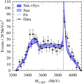
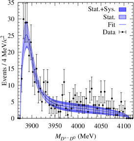
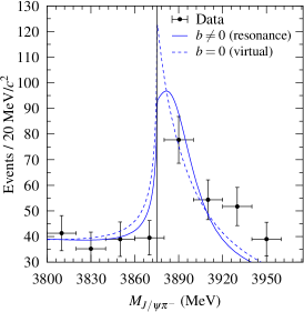
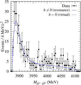
Figure 2: Invariant mass distributions for $J/\psi\pi^{-}$ in the decay $Y(4260)\to J/\psi\pi\pi$ (left panels) Ablikim:2013mio and for $\bar{D}^{\ast-}D^{0}$ in the decay $Y(4260)\to\bar{D}^{\ast}D\pi$ (right panels) Ablikim:2015swa . The top panels show the results for the fit $b\neq 0$, $\Lambda_{2}=0.5\ \text{GeV}$. The inner and lighter error bands reflect the statistical uncertainties, while the outer and darker bands include also the systematic ones. In the bottom panels, the two fits $b=0$ and $b\neq 0$ are compared (without error bands) for the case $\Lambda_{2}=0.5\ \text{GeV}$. In the $J/\psi\pi^{-}$ spectrum, the $\bar{D}^{\ast}D$ threshold is marked with a vertical black line.

We have three free parameters directly related to our $T$-matrix ($C_{1Z}$, $\widetilde{C}$, and $b$), and six ($B_{1}$, $d_{1}$, $\alpha$, $\beta$ and $K_{1,2}$) related to the background and the overall normalization. These nine free parameters are adjusted to reproduce the data of Refs. Ablikim:2013mio ; Ablikim:2015swa (a total of 104 data points). In this work, two errors are given. The first error is statistical and it is computed from the hessian matrix of the $\chi^{2}$ merit function. The second error is systematic, and to estimate it we have considered two different uncertainty sources. First, we have varied the $J/\psi\pi$ background function [Eq. (13)] and used other smooth functions. The second source of uncertainties is related to the tail of the $\bar{D}^{\ast}D$ spectrum, and it is estimated as follows. The central value of the parameters is computed by fitting this spectrum up to $\sqrt{s}=4025\ \text{MeV}$. Then, we vary this limit between $\sqrt{s}=3975\ \text{MeV}$ and $m_{+}$ (the maximum allowed invariant mass), and repeat the fit. In all cases, we find statistically acceptable fits and the difference between the new fitted parameters and the central ones is used to determine the systematic error. The same method is applied to estimate the systematic error of our predictions for the spectra and the mass and width of the $Z_{c}$ state, to be presented below.

We perform four different fits, corresponding to the two cases of keeping the parameter $b$, which controls the energy dependence of the $\bar{D}^{*}D$ potential, free or set to zero, and for each of these, we choose $\Lambda_{2}$ to be $0.5$ or $1\ \text{GeV}$ HQSSFormalism . Results from the four fits are compiled in Table 1, where only the parameters that are directly related to our $T$-matrix are shown. One first notes that the reduced $\chi^{2}$ is very close to unity in all four cases. Indeed, the description of the experimental spectra is very good in all cases, as can be seen in the top panels of Fig. 2, where the results from one of the fits ($b$ free and $\Lambda_{2}=0.5\ \text{GeV}$) are shown and confronted with the data. In particular, the effect of the $Z_{c}$ is nicely reproduced in the $\bar{D}^{\ast}D$ spectrum above threshold and in the $J/\psi\pi$ spectrum around the $\bar{D}^{\ast}D$ threshold. Its reflection can also be appreciated in the $J/\psi\pi$ distribution around $3.5\ \text{GeV}$. The other fits lead to results similar to those shown in Fig. 2. The largest differences can be found in the $\bar{D}^{\ast}D$ spectrum between the $b\neq 0$ and $b=0$ cases, which are compared for $\Lambda_{2}=0.5\ \text{GeV}$ in the bottom right panel of the same figure. In any case, we see that we are able to simultaneously reproduce the two available BESIII data sets related to the $Z^{\pm}_{c}(3900)/Z^{\pm}_{c}(3885)$ state with a single structure for the very first time.

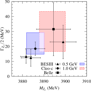
Figure 3: Comparision of the $Z_{c}$ resonance pole positions determined in this work for two values of the cutoff $\Lambda_{2}$ with the experimental determinations of Refs. Ablikim:2013mio ; Ablikim:2013xfr ; Ablikim:2015swa ; Liu:2013dau ; Xiao:2013iha . The shaded areas take into account our statistical and systematic uncertainties (added in quadratures). The numerical values are shown in Table 2.

Since we have a good description of the data where the $Z_{c}$ peak is seen, we next study the pole structure of the $T$-matrix. Poles can be found in different Riemann sheets of the $T$-matrix, which are reached through analytical continuation of the $G$ functions in Eqs. (4) and (5). The $(\eta_{1}\eta_{2})$ Riemann sheet is defined with the following replacements:

$$G_{1}(E) \rightarrow G_{1}(E)+\eta_{1}i\frac{q_{1}(E)}{4\pi E}~{},$$ (14)

$$G_{2}(E) \rightarrow G_{2}(E)+\eta_{2}i\frac{q_{2}(E)}{4\pi(m_{D}+m_{D}^{\ast})}~{}.$$ (15)

In this way, the physical sheet would be denoted as $(00)$.

We define the mass and the width of the $Z_{c}$ from its pole position, $\sqrt{s}=M_{Z_{c}}-i\Gamma_{Z_{c}}/2$. For the case $b\neq 0$, we find poles on the $(11)$ Riemann sheet, which is connected to the physical one above the $D\bar{D}^{\ast}$ threshold, at energies shown in Table 2. The real part of these energies is clearly above threshold, so they correspond to a resonance, which really (physically) exists as an unstable particle. In Fig. 3, we compare the pole position obtained in this work for the $Z_{c}$ resonance with the experimental determinations of Refs. Ablikim:2013mio ; Liu:2013dau ; Xiao:2013iha ; Ablikim:2013xfr ; Ablikim:2015swa . Such comparisons are also displayed in Table 2. There is a good agreement within errors, and the small differences can be traced back to the fact that these experimental analyses used a Breit-Wigner parametrization which is not good around a strongly-coupled threshold.

For the case $b=0$, however, the situation is quite different. While the description of the experimental data is still quite good with $\chi^{2}/\text{d.o.f.}\in[1.3,1.4]$, the pole in this case is located below threshold, with a small imaginary part (around $8\ \text{MeV}$), and in the $(01)$ Riemann sheet. If the $J/\psi\pi$ channel were now switched off ($\widetilde{C}=0$), this pole would move into the real axis in the unphysical Riemann sheet of the elastic amplitude $T_{22}$. In this sense, the obtained pole does not qualify as a resonance, and we see it as a virtual or anti-bound $D\bar{D}^{*}$ state. It does not correspond to a particle in the sense that its wave function, unlike that of a bound state, is not localized. However, it produces observable effects at the $D\bar{D}^{\ast}$ threshold similar to those produced by a near threshold resonance or bound state. Indeed, scattering experiments alone, in principle, cannot distinguish between virtual and bound states, but the difference is not a purely academic one since they can produce different line shapes in inelastic open channels Hanhart:2007yq . The line shapes of a virtual state and a near-threshold resonance are different since the former is peaked exactly at the threshold while the latter, in principle, is above. This can be seen in the left bottom panel of Fig. 2 where the $J\psi\pi^{-}$ spectrum for the two fits $b=0$ and $b\neq 0$ are shown (for the case $\Lambda_{2}=0.5\ \text{GeV}$). Although the two curves are different, each one would approximately lie within the error band of the other. Clearly, very precise data with a good energy resolution and small bin size are necessary to distinguish among them.

Without taking sides, and given that both natures for the $Z_{c}$ structure (resonance or virtual state) arise in fits of good quality, it must be stated that the experimental information available at this time cannot fully discriminate between both scenarios and, hence, claims about the $Z_{c}$ structure should be made with caution. Nevertheless, the resonance scenario seems to be statistically slightly preferred. It is also clear that more experimental information is needed to elaborate on the nature of $Z_{c}$. In particular, the spectrum of $J/\psi\pi$ with narrower bins would be highly desirable to have a good resolution on its line shape. If it is finally shown to be a virtual state, then it cannot be a tetraquark, since it does not correspond to a normal particle, and it can only have a hadronic molecular nature, in the sense that it appears only because of the $D\bar{D}^{*}$ interaction.

Summarizing, we have studied the two decays ($Y(4260)\to J/\psi\pi^{+}\pi^{-},D^{\ast-}D^{0}\pi^{+}$) in which the $Z^{\pm}_{c}$ resonant-like structure is seen. We have presented the first simultaneous study of the invariant mass distributions of the $J/\psi\pi$ and $\bar{D}^{\ast}D$ channels with fully unitarized amplitudes. We find that these data sets are well reproduced in two different scenarios. In the first one, in which there is an energy dependence in the $\bar{D}^{\ast}D\to\bar{D}^{\ast}D$ potential, the $Z_{c}$ appears as a dynamically generated $\bar{D}^{\ast}D$ resonance. In the second one, however, when the aforementioned energy dependence is not allowed, it appears as a virtual state, with the pole located below the $D\bar{D}^{*}$ threshold. In any case, it is demonstrated that both data sets can be reproduced with only one $Z_{c}$ state, so that the two experimentally observed structures $Z^{\pm}_{c}(3900)$ and $Z_{c}^{\pm}(3885)$, in different channels, are proven to correspond to the same state. Moreover, both fits do not allow a $\bar{D}^{*}D$ bound state solution. Since the virtual state can only be of hadronic-molecule type, it is really important to discriminate between these two scenarios. For that purpose, one needs a very precise measurement of the line shapes around, in particular slightly above, the $D\bar{D}^{*}$ threshold. Such a measurement is foreseen when more data are collected at BESIII.

References

- (1) M. Ablikim et al. [BESIII Collaboration], Phys. Rev. Lett. 110, 252001 (2013).
- (2) Z. Q. Liu et al. [Belle Collaboration], Phys. Rev. Lett. 110, 252002 (2013).
- (3) T. Xiao, S. Dobbs, A. Tomaradze and K. K. Seth, Phys. Lett. B 727, 366 (2013)
- (4) M. Ablikim et al. [BESIII Collaboration], Phys. Rev. Lett. 112, 022001 (2014).
- (5) M. Ablikim et al. [BESIII Collaboration], Phys. Rev. D 92, 092006 (2015).
- (6) M. Ablikim et al. [BESIII Collaboration], Phys. Rev. Lett. 115, 112003 (2015).
- (7) F.-K. Guo, C. Hanhart, Q. Wang and Q. Zhao, Phys. Rev. D 91, 051504 (2015).
- (8) M. B. Voloshin, Phys. Rev. D 87, 091501 (2013).
- (9) Q. Wang, C. Hanhart and Q. Zhao, Phys. Rev. Lett. 111, 132003 (2013).
- (10) F.-K. Guo, C. Hidalgo-Duque, J. Nieves and M. P. Valderrama, Phys. Rev. D 88, 054007 (2013).
- (11) E. Wilbring, H.-W. Hammer and U.-G. Meißner, Phys. Lett. B 726, 326 (2013); Y. Dong, A. Faessler, T. Gutsche and V. E. Lyubovitskij, Phys. Rev. D 88, 014030 (2013); J. R. Zhang, Phys. Rev. D 87, 116004 (2013); H. W. Ke, Z. T. Wei and X. Q. Li, Eur. Phys. J. C 73, 2561 (2013); F. Aceti et al., Phys. Rev. D 90, 016003 (2014); J. He, Phys. Rev. D 92, 034004 (2015).
- (12) E. Braaten, Phys. Rev. Lett. 111, 162003 (2013); J. M. Dias, F. S. Navarra, M. Nielsen and C. M. Zanetti, Phys. Rev. D 88, 016004 (2013); L. Maiani, F. Piccinini, A. D. Polosa and V. Riquer, Phys. Rev. D 89, 114010 (2014); A. Esposito, A. L. Guerrieri, F. Piccinini, A. Pilloni and A. D. Polosa, Int. J. Mod. Phys. A 30, 1530002 (2014); C. F. Qiao and L. Tang, Eur. Phys. J. C 74, 3122 (2014); Z. G. Wang and T. Huang, Phys. Rev. D 89, 054019 (2014); C. Deng, J. Ping and F. Wang, Phys. Rev. D 90, 054009 (2014).
- (13) D. Y. Chen, X. Liu and T. Matsuki, Phys. Rev. D 88, 036008 (2013); E. S. Swanson, Phys. Rev. D 91, 034009 (2015).
- (14) M. Cleven, F.-K. Guo, C. Hanhart, Q. Wang and Q. Zhao, Phys. Rev. D 92, 014005 (2015).
- (15) S. Prelovsek and L. Leskovec, Phys. Lett. B 727, 172 (2013); S. Prelovsek, C. B. Lang, L. Leskovec and D. Mohler, Phys. Rev. D 91, 014504 (2015); Y. Chen et al., Phys. Rev. D 89, 094506 (2014); S. H. Lee et al. [Fermilab Lattice and MILC Collaborations], arXiv:1411.1389 [hep-lat].
- (16) E. Swanson, Int. J. Mod. Phys. A 21, 733 (2006); F. Close, C. Downum and C. E. Thomas, Phys. Rev. D 81, 074033 (2010); G. J. Ding, Phys. Rev. D 79, 014001 (2009); M. T. Li, W. L. Wang, Y. B. Dong and Z. Y. Zhang, arXiv:1303.4140 [nucl-th].
- (17) K. Yokokawa, S. Sasaki, T. Hatsuda and A. Hayashigaki, Phys. Rev. D 74, 034504 (2006); L. Liu, H. W. Lin and K. Orginos, PoS LATTICE 2008, 112 (2008).
- (18) X. H. Liu, F.-K. Guo and E. Epelbaum, Eur. Phys. J. C 73, 2284 (2013).
- (19) C. Hanhart, Y. S. Kalashnikova, P. Matuschek, R. V. Mizuk, A. V. Nefediev and Q. Wang, Phys. Rev. Lett. 115, 202001 (2015).
- (20) J. Nieves and M. P. Valderrama, Phys. Rev. D 86, 056004 (2012); C. Hidalgo-Duque, J. Nieves and M. P. Valderrama, Phys. Rev. D 87, 076006 (2013).
- (21) E. Epelbaum, H.-W. Hammer and U.-G. Meißner, Rev. Mod. Phys. 81, 1773 (2009).
- (22) M. Albaladejo, F.-K. Guo, C. Hidalgo-Duque, J. Nieves and M. P. Valderrama, Eur. Phys. J. C 75, 547 (2015).
- (23) F.-K. Guo, C. Hanhart, U.-G. Meißner, Q. Wang and Q. Zhao, Phys. Lett. B 725, 127 (2013).
- (24) C. Hanhart, Y. S. Kalashnikova, A. E. Kudryavtsev and A. V. Nefediev, Phys. Rev. D 76, 034007 (2007).