Composite and elementary nature of a resonance in the sigma model

Abstract

We analyze the mixing nature of the low-lying scalar resonance consisting of the $\pi\pi$ composite and the elementary particle within the sigma model. A method to disentangle the mixing is formulated in the scattering theory with the concept of the two-level problem. We investigate the composite and elementary components of the $\sigma$ meson by changing a mixing parameter. We also study the dependence of the results on model parameters such as the cut-off value and the mass of the elementary $\sigma$ meson.

I Introduction

Understanding the internal structure of hadrons is an important issue to clarify various properties of hadrons. The purpose of the present work is to shed light upon the nature of hadrons whether they are composed of quarks and gluons confined in a single region or rather develop hadronic molecular like structure. In this paper, the former is referred to as the elementary hadron and the latter to as the hadronic composite. Here we assume that the above two configurations are well distinguished, though in general the distinction is not perfect.

It has been suggested that some hadronic resonances could well develop the structure of hadronic composite. Especially, the nature of the $\sigma$ meson, which is now listed in the table of the Particle Data Group (PDG) Beringer et al. (2012), has been a longstanding problem Basdevant and Lee (1970); Achasov and Shestakov (1994); Törnqvist and Roos (1996); Harada et al. (1996, 1997); Oller and Oset (1997); Igi and Hikasa (1999); Oller et al. (1999); Hyodo et al. (2010). There are various approaches to describe the lowest lying scalar meson by the $q\bar{q}$ state, the four-quark state, the $\pi\pi$ molecular state, and so on. In general, if more than one quantum state is allowed for a given set of quantum numbers, hadronic resonant states are unavoidably mixtures of these states. Therefore, an important issue is to clarify how these components are mixed in a physical hadron.

In this paper we investigate the mixing nature of the $\sigma$ meson which is treated as a superposition of the elementary $\sigma$ meson, and a $\pi\pi$ composite state within the framework of the sigma model. In our previous study Nagahiro et al. (2011), we have proposed a method to disentangle the mixture of hadrons having the elementary component and that of hadronic composite by taking the $a_{1}(1260)$ axial-vector meson as an example. The method makes use of the concept of the two-level problem, and can be generally applied to other mixed systems if the interaction is given between the elementary component and constituents of the composite state. The $a_{1}$ meson was a good example because we have a model Bando et al. (1988) involving the elementary $a_{1}$ field as well as $\pi$ and $\rho$ fields developing the $\pi\rho$ composite state Roca et al. (2005); Nagahiro et al. (2009).

The sigma model also provides us with a platform to study the mixing nature of resonances. In the so-called nonlinear sigma model, the $\sigma$ meson is introduced as a dynamically generated resonance through the non-perturbative hadron dynamics Oller and Oset (1997). In that model Lagrangian, the degree of freedom of the elementary $\sigma$ fields is freezed out by taking the mass of the elementary $\sigma$ infinite, and instead, the four-pion contact interaction becomes attractive to develop the $\sigma$ state as a $\pi\pi$ composite resonance.

In contrast, in this article, we keep the mass of the elementary $\sigma$ field finite and treat it as an independent degree of freedom. Because the four-pion interaction is still attractive, the unitarized amplitude of this interaction develops a pole for the dynamically generated resonance, which is another degree of freedom for the $\sigma$ meson. In the Bethe-Salpeter equation of the sigma model, the two degrees of freedom couple, and the resulting solution is expressed as a superposition of the two. In this way, we investigate the mixing nature of the $\sigma$ meson by applying the method given in Ref. Nagahiro et al. (2011).

This article is organized as follows. In Sec. II we give the formulation to obtain the non-perturbative scattering amplitude based on the sigma model. In Sec. III, we introduce the method to disentangle mixture by means of the two-level problem. We show our numerical results and give associated discussions in Sec. IV. Finally, Sec. V is devoted to conclude this article.

II formalism

II.1 tree level amplitude

Our discussion of the $\pi\pi$ scattering is based on the sigma model. The Lagrangian Donoghue et al. (1992) is given by

$${\cal L}=\frac{1}{4}{\rm Tr}\left(\partial_{\mu}\Sigma\partial^{\mu}\Sigma^{\dagger}\right)+\frac{\mu^{2}}{4}{\rm Tr}\left(\Sigma^{\dagger}\Sigma\right)\\ -\frac{\lambda}{16}\left[{\rm Tr}\left(\Sigma^{\dagger}\Sigma\right)\right]^{2}+a{\rm Tr}\left(\Sigma^{\dagger}+\Sigma\right)\ .$$ (1)

Here in the standard notation the chiral field is parameterized as $\Sigma=\sigma+i\vec{\tau}\cdot\vec{\pi}$, and so the first term of (1) gives the properly normalized kinetic terms for $\sigma$ and $\pi$,

$$\frac{1}{2}(\partial_{\mu}\sigma\partial^{\mu}\sigma+\partial_{\mu}\vec{\pi}\cdot\partial^{\mu}\vec{\pi})\ .$$ (2)

The second and third terms of (1) give the mass and the four-point interaction terms of $\sigma$ and $\pi$, respectively, where $\mu$ is their common mass and $\lambda$ the coupling constant. When chiral symmetry is spontaneously broken, the potential, the sum of the second and third terms, takes the minimum at a finite expectation value of ${\sigma=}\langle\sigma\rangle\equiv f_{\pi}$, where $f_{\pi}$ is the pion decay constant. The physical $\sigma$ field is then expanded around this vacuum, such that $\sigma\rightarrow f_{\pi}+\sigma$. The last term of (1) is for explicit breaking of chiral symmetry and gives the physical mass for the pion after the spontaneous chiral symmetry breaking.

In this study, we employ the nonlinear representation for the chiral field as

$$\Sigma=(f_{\pi}+\sigma)U,\ \ U=\exp\left(\frac{i\vec{\tau}\cdot\vec{\pi}}{f_{\pi}}\right).$$ (3)

This provides interaction terms for $\pi$ and $\sigma$ including three and four-point interactions as,

$${\cal L}_{\rm int}=\frac{1}{6f_{\pi}^{2}}\left\{\left(\partial_{\mu}\vec{\pi}\cdot\vec{\pi}\right)^{2}-(\partial_{\mu}\vec{\pi}\cdot\partial^{\mu}\vec{\pi})(\vec{\pi}\cdot\vec{\pi})\right\}\\ +\frac{m_{\pi}^{2}}{24f_{\pi}^{2}}(\vec{\pi}\cdot\vec{\pi})^{2}+\frac{1}{f_{\pi}}\sigma\,\partial_{\mu}\vec{\pi}\cdot\partial^{\mu}\vec{\pi}-\frac{m_{\pi}^{2}}{2f_{\pi}}\sigma\vec{\pi}\cdot\vec{\pi}.$$ (4)

The three parameters, $\mu$, $\lambda$, and $a$, in the Lagrangian (1) are determined by the three inputs, $f_{\pi}=92.4$ MeV, $m_{\pi}=138$ MeV (isospin-averaged) and $m_{0}$. The mass of the elementary $\sigma$ field, $m_{0}$, is varied in the present study, but we shall start with the value $m_{0}=550$ MeV.

The $\pi\pi$ scattering amplitude at the tree level is determined in terms of a single function $A(s,t,u)$ by

$$T_{\alpha\beta,\gamma\delta}^{\rm tree}=A(s,t,u)\delta_{\alpha\beta}\delta_{\gamma\delta}+A(t,s,u)\delta_{\alpha\gamma}\delta_{\beta\delta}\\ +A(u,t,s)\delta_{\alpha\delta}\delta_{\beta\gamma}\ ,$$ (5)

where $\alpha$, $\beta$, $\gamma$, $\delta$ denote the isospin components of the pions. The amplitude with isospin $I=0$ for the $\sigma$ channel is given by

$$T^{\rm tree}_{I=0}=3A(s,t,u)+A(t,s,u)+A(u,t,s)\ .$$ (6)

The function $A(s,t,u)(\equiv A(s))$ is obtained from the interaction Lagrangian (4) as

$$A(s)=-\frac{1}{f_{\pi}^{2}}(s-m_{\pi}^{2})+\frac{1}{f_{\pi}^{2}}(s-m_{\pi}^{2})^{2}\frac{1}{s-m_{0}^{2}}\ ,$$ (7)

where the first term comes from the four-pion contact interaction as depicted in Fig. 1(a) and the second term the elementary $\sigma$-exchange in $s$-channel (we refer to it as “$\sigma$-pole” hereafter) as in Fig. 1(b).

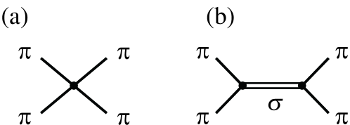
Figure 1: Feynman diagrams contributing for the function $A(s)$ in Eq. (7).

The $s$-wave amplitude for the $\sigma$ meson can be projected out,

$$v(s)=\frac{1}{2}\int^{1}_{-1}dx\ T^{\rm tree}_{I=0}(s,t(x),u(x))P_{\ell=0}(x)\ ,$$ (8)

in the center-of-mass frame. The result of the projection is given by

$$v(s)=-\frac{1}{f_{\pi}^{2}}(2s-m_{\pi}^{2})+\frac{3}{f_{\pi}^{2}}(s-m_{\pi}^{2})^{2}\frac{1}{s-m_{0}^{2}}\\ -\frac{1}{f_{\pi}^{2}}\left[(s-2m_{0}^{2})-\frac{2(m_{\pi}^{2}-m_{0}^{2})^{2}}{s-4m_{\pi}^{2}}\ln\left(\frac{m_{0}^{2}}{m_{0}^{2}-4m_{\pi}^{2}+s}\right)\right]\ ,$$ (9)

where we have used the relation $s+t+u=4m_{\pi}^{2}$ for on-shell amplitudes. Here the first term in Eq. (9) is obtained by the four-pion contact interaction, the second term the $\sigma$-pole, and the last term the $\sigma$-exchange in $t$- and $u$-channels.

II.2 Unitarized scattering amplitude

The tree level amplitude projected on the $s$-wave, $v(s)$, is now used as a potential (interaction kernel) in the Bethe-Salpeter (BS) equation to find the $\sigma$ meson as a resonance of $\pi\pi$ scattering. In literatures, the process is often referred to as unitarization. The resulting unitarized amplitude $t$ is then given by

$$t = v+vGt$$ (10)

$$= v+vGv+vGvGv+\cdots\ ,$$

where infinite set of diagrams are summed up as depicted in Fig. 2.

Figure 2: Sum of the infinite set of diagrams that contributes to the meson-meson scattering amplitude (10). If a pole is developed, then it is interpreted as the composite state in Eq. (22) which is depicted as in the right-hand-side.

In general this is an integral equation, but in many recent applications, the on-shell factorization is employed to reduce it to an algebraic equation. Thus the resulting amplitude $t$ is obtained as

$$t=\frac{1}{v^{-1}-G}\ ,$$ (11)

where $G$ denotes the integrated $\pi\pi$ two-body propagator as

$$G(\sqrt{s})=\frac{i}{2}\int\frac{d^{4}k}{(2\pi)^{4}}\frac{1}{(P-k)^{2}-m_{\pi}^{2}+i\epsilon}\frac{1}{k^{2}-m_{\pi}^{2}+i\epsilon}.$$ (12)

Here $P$ is the total momentum in the center-of-mass frame, $P=(\sqrt{s},0,0,0)$, and the factor 1/2 is introduced as the symmetry factor for the identical particles. We evaluate the regularized loop function in Eq. (12) by the dimensional regularization scheme as,

$$G(\sqrt{s}) = \frac{1}{32\pi^{2}}\left[a(\mu)+\ln\frac{m_{\pi}^{2}}{\mu^{2}}\right.$$

$$+\left.\frac{2q}{\sqrt{s}}\left\{\ln(s+2q\sqrt{s})-\ln(s-2q\sqrt{s})-\pi i\right\}\right],$$

where $\mu$ is the renormalization scale. $a(\mu)$ is the subtraction constant at the scale $\mu$, and the three-momentum $q$ of two pions in the center-of-mass frame for a given $s$ is obtained by,

$$q=\frac{1}{2\sqrt{s}}\lambda^{1/2}(s,m_{\pi}^{2},m_{\pi}^{2})\ ,$$ (14)

with $\lambda(x,y,z)=x^{2}+y^{2}+z^{2}-2xy-2yz-2zx$. We first use the natural value for $a(\mu)$ Hyodo et al. (2008, 2010). Later, we employ another form regularized by the three-dimensional cut-off as

$$G(\sqrt{s})=\frac{1}{4\pi^{2}}\int_{0}^{\Lambda}\frac{k^{2}dk}{E_{\pi}(s-4E_{\pi}^{2}+i\epsilon)}\ ,$$ (15)

where $E_{\pi}=\sqrt{k^{2}+m_{\pi}^{2}}$, to investigate cut-off dependence of various properties of the $\sigma$ meson.

If the potential $v$ is sufficiently attractive, the amplitude $t$ in Eq. (11) develops a pole corresponding to a bound or resonant state at the energy satisfying $v^{-1}-G=0$. When we need to find a bound state pole below the threshold, we use the loop function in the first Riemann sheet ($G^{I}$) with Im $q>0$. In the present study in the nonlinear representation, the four-pion interaction is attractive and the pole appears above the two pion threshold in the second Riemann sheet as a resonant state, which can be interpreted as the $\pi\pi$ composite $\sigma$ meson Oller and Oset (1997). The loop function in the second Riemann sheet ($G^{II}$) can be obtained by

$$G^{II}(\sqrt{s})=G^{I}(\sqrt{s})+i\frac{q}{8\pi\sqrt{s}}$$ (16)

with Im $q>0$ Roca et al. (2005). Here, we recall that the generation of the composite $\sigma$ state through the non-perturbative dynamics is a feature of the nonlinear representation of the sigma model.

In this study, we split the tree-level amplitude in Eq. (9) into two parts, the “contact” and “$\sigma$-pole” terms as,

$$v = v_{\rm con}+v_{\rm pole}$$ (17)

$$v_{\rm con} = -\frac{1}{f_{\pi}^{2}}\left[3s-m_{\pi}^{2}-2m_{0}^{2}\right.$$ (18)

$$-\left.\frac{2(m_{\pi}^{2}-m_{0}^{2})^{2}}{s-4m_{\pi}^{2}}\ln\left(\frac{m_{0}^{2}}{m_{0}^{2}-4m_{\pi}^{2}+s}\right)\right]$$

$$v_{\rm pole} = \frac{3}{f_{\pi}^{2}}(s-m_{\pi}^{2})^{2}\frac{1}{s-m_{0}^{2}}\ .$$ (19)

The “contact” interaction $v_{\rm con}$ contains not only the four-pion interaction but also the contribution of the $\sigma$-exchange in $t$- and $u$-channels. The latter slightly modifies the attractive potential coming from the four-pion interaction, but the total attraction of $v_{\rm con}$ is still strong enough such that the unitarized amplitude $t_{\rm composite}$

$$t_{\rm composite}=\frac{v_{\rm con}}{1-v_{\rm con}G}$$ (20)

develops a resonance pole. In the present work, we identify the $\sigma$ meson generated in Eq. (20) with the composite $\sigma$ meson. In contrast, $v_{\rm pole}$ has the elementary $\sigma$-pole. In this way, we have defined two “seeds” of the $\sigma$ meson having different origins.

A similar decomposition of the amplitude into the contact and pole terms was also considered in Ref. Hyodo et al. (2010). There the contact interaction $T_{\rm tree}^{\rm(contact)}$ was chosen to be repulsive, while the $v_{\rm con}$ in Eq. (18) is attractive. This difference comes from the definition of the “$\sigma$-pole term”, namely, the authors in Ref. Hyodo et al. (2010) isolate the $\sigma$-pole in the linear representation of the sigma model, while we isolate it in the nonlinear representation. In the linear representation, the $\sigma\pi\pi$ coupling does not depend on the energy, while in the nonlinear representation the $\sigma\pi\pi$ coupling does depend on the energy. Furthermore the four-pion interaction in the linear representation is repulsive, and hence one does not have a composite $\sigma$-pole.

Substituting Eq. (17) as the potential into the BS equation we obtain the full scattering amplitude in $s$-wave as

$$t=\frac{v_{\rm con}+v_{\rm pole}}{1-(v_{\rm con}+v_{\rm pole})G}.$$ (21)

In the present work, we analyze this full scattering amplitude in detail to study the nature of the $\sigma$ meson.

III reduction to the two-level problem

The two bases of composite and elementary natures mix in the solution of the full amplitude (21). The situation is similar to a two-level problem in the quantum mechanics. This idea has been employed in Ref. Nagahiro et al. (2011), where the mixing nature of $a_{1}(1260)$ axial vector meson consisting of $\pi\rho$ composite and elementary $a_{1}$ meson has been investigated. There two physical $a_{1}$ poles are found as superpositions of the two basis states. One of them is identified with the experimentally observed $a_{1}$ meson, which is found to have comparable amount of the elementary $a_{1}$ component to that of the $\pi\rho$ composite.

We apply this method to the study of the $\sigma$ meson. Here we show details of the formulation which have been omitted in Ref. Nagahiro et al. (2011). We first express the amplitude $t_{\rm composite}$ by an $s$-channel pole term as

$$t_{\rm composite}\equiv g_{R}(s)\frac{1}{s-s_{p}}g_{R}(s)\ ,$$ (22)

where $s_{p}$ is the pole position of the amplitude $t_{\rm composite}$. In this form, we can interpret $(s-s_{p})^{-1}$ as the one-particle propagator of the composite $\sigma$ meson. Furthermore, $g_{R}(s)$ defined by Eq. (22) is interpreted as the vertex function of the composite $\sigma$ meson to two pions in the neighborhood of the pole, $s\sim s_{p}$. However, as $s$ is getting apart from $s_{p}$ this interpretation is no longer appropriate, where instead it should be reinterpreted together with background contribution.

Having the form of Eq. (22), we can express the full scattering amplitude (21) by

$$t=(g_{R},g)\frac{1}{\hat{D}_{0}^{-1}-\hat{\Sigma}}\begin{pmatrix}g_{R}\\ g\end{pmatrix}\ ,$$ (23)

where

$$\hat{D}_{0}^{-1}=\begin{pmatrix}s-s_{p}&0\\ 0&s-m_{0}^{2}\end{pmatrix},\ \hat{\Sigma}=\begin{pmatrix}0&g_{R}Gg\\ gGg_{R}&gGg\end{pmatrix}\ .$$ (24)

Here $g$ is the coupling of $\sigma\pi\pi$ as $g^{2}=3(s-m_{\pi}^{2})^{2}/f_{\pi}^{2}$. The detailed derivation is given in Appendix A. The diagonal elements of $\hat{D}_{0}$ are the free propagators of two different $\sigma$’s, one for the composite $\sigma$ and the other for the elementary $\sigma$. The matrix $\hat{\Sigma}$ expresses the self-energy and mixing interaction between the two $\sigma$’s.

Now, the matrix

$$\hat{D}=\frac{1}{\hat{D}_{0}^{-1}-\hat{\Sigma}}$$ (25)

is the full propagators of the physical states represented by the two bases of the composite and elementary $\sigma$ mesons. The diagonal $D^{ii}$ correspond to full propagators of the composite and elementary $\sigma$ mesons as shown in Fig. 3, which express each $\sigma$ meson acquires the quantum effects through the mixing from the other as well as the self-energy. In this manner we can study the mixing nature of the $\sigma$ meson by analyzing the properties of $\hat{D}$.

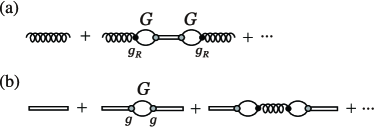
Figure 3: Full propagators of (a) composite and (b) elementary $\sigma$ mesons defined in Eq. (25). The solid line indicates the $\pi$ propagator, while the curly and double lines are those of the composite and elementary $\sigma$ mesons.

The important feature of the propagators in Eq. (25) is that they have poles $m^{*}$ exactly at the same positions as the full amplitude $t$ in Eq. (21). The residues of the diagonal elements $D^{ii}$ are obtained by

$$z^{ii}=\frac{1}{2\pi i}\oint_{\gamma}D^{ii}(s)ds\ ,\ \ (i=1,2)$$ (26)

where $\gamma$ is a closed circle around the pole $m^{*}$. They are the wave function renormalizations for the basis states $i$ and then they have information on the mixing rate of the physical resonant pole. For instance, $D^{11}$ is the full propagator of the composite $\sigma$ meson, and its residue $z^{11}$ has the meaning of the probability of finding the composite $\sigma$ component in the resulting state. So we schematically express the physical $\sigma$ state $|\sigma\rangle_{\rm phys}$ as

$$|\sigma\rangle_{\rm phys}=\sqrt{z^{11}}|1\rangle+\sqrt{z^{22}}|2\rangle$$ (27)

with $|1\rangle$ and $|2\rangle$ the composite and elementary states.

The residue $z^{22}$, the wave function renormalization factor for the elementary $\sigma$, can be computed also by

$$z^{22}=\left(1-\left.\frac{d\Pi(s)}{ds}\right|_{s={m^{*}}^{2}}\right)^{-1},$$ (28)

where $\Pi(s)$ denotes the self-energy for the elementary $\sigma$ given by,

$$\Pi(s)=3\frac{(s-m_{\pi}^{2})^{2}}{f_{\pi}^{2}}\frac{G(\sqrt{s})}{1-v_{\rm con}G(\sqrt{s})}.$$ (29)

The wave function renormalization factor is often used to study the “compositeness” of the physical state. The relation between the compositeness condition discussed in Refs. Weinberg (1965); Lurie and Macfarlane (1964); *Lurie:book; Hyodo et al. (2012) and the $z^{22}$ in this two-level problem will be investigated elsewhere Nagahiro and Hosaka .

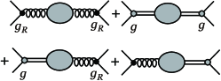
Figure 4: Full scattering amplitude in terms of the full propagators $\hat{D}$. The first two diagrams denote the amplitudes through the full propagators of composite and elementary $\sigma$ mesons ($D^{11}$ and $D^{22}$), respectively, and the last two diagrams those of off-diagonal propagators ($D^{21}$ and $D^{12}$).

Now, we can write the full scattering amplitude around a pole $m^{*}$ by using the components of the full propagator $\hat{D}$ as,

$$t \simeq g_{R}\frac{z^{11}}{s-{m^{*}}^{2}}g_{R}+g\frac{z^{22}}{s-{m^{*}}^{2}}g$$

$$+ g\frac{z^{21}}{s-{m^{*}}^{2}}g_{R}+g_{R}\frac{z^{12}}{s-{m^{*}}^{2}}g$$

as shown in Fig. 4. Here, the residue of the off-diagonal propagator, $z^{12}(=z^{21})$, has the following relation with $z^{11}$ and $z^{22}$ as

$$(z^{12})^{2}=z^{11}z^{22}\ .$$ (31)

Therefore the full amplitude near the pole can be expressed by

$$t=(g_{R}\sqrt{z^{11}}+g\sqrt{z^{22}})^{2}\frac{1}{s-{m^{*}}^{2}}.$$ (32)

In a simple Yukawa theory where only one “seed” state exists, the scattering amplitude is given by

$$T_{\rm Yukawa}=g_{0}^{2}Z\frac{1}{s-{M^{*}}^{2}}\ ,$$ (33)

where $g_{0}$ is the original Yukawa coupling constant and $Z^{1/2}$ the wave function renormalization. Comparing Eqs. (32) and (33), we realize that the renormalized coupling constant $g_{0}Z^{1/2}$ is now replaced by the sum of those of the two bases $g_{R}\sqrt{z^{11}}$ and $g\sqrt{z^{22}}$. In this form of Eq. (32), we can clearly see that the contributions from the original basis states to the full scattering amplitude is determined by probabilities of finding their components in the physical state multiplied by their couplings to the scattering state.

IV Numerical Results

IV.1 pole-flow in complex-energy plane

parameter	pole position (in unit of MeV)	property of pole (mark in Figs. 5 and/or 6)
$x=0$	$360.8-354.6i$	naive-composite $\sigma$ generated by four-pion interaction ($\blacksquare$)
	$550-0i$	elementary $\sigma$ (${\circ}$)
$x=1$	$420.5-128.0i$	physical state (•)
$X=0$	$390.7-308.4i$	composite $\sigma$ generated by $v_{\rm con}$ ($\blacktriangle$)
	$550-0i$	elementary $\sigma$ (${\circ}$)
$X=1$	$420.5-128.0i$	physical state (•)

Table 1: Pole positions of the full propagator $\hat{D}$ when the mass of the elementary $\sigma$ meson $m_{0}=550$ MeV is employed.

IV.1.1 Parameterization-(I)

Now, the full scattering amplitude in Eq. (21) or Eq. (23) and hence the full propagator can be calculated numerically. We first investigate the pole position of $\hat{D}$ in complex-energy plane by varying the coupling strength of the $\sigma\pi\pi$ three-point vertex. To this end, we introduce the parameter $x$ as,

$$A(s,t,u)=-\frac{1}{f_{\pi}^{2}}(s-m_{\pi}^{2})+x\frac{(s-m_{\pi}^{2})^{2}}{f_{\pi}^{2}}\frac{1}{s-m_{0}^{2}}$$ (34)

and the same for $A(t,s,u)$ and $A(u,t,s)$ as in Ref. Hyodo et al. (2010). We call this “parameterization-(I)”. In Fig. 5, we show the resulting pole-flow in complex-energy plane by changing the parameter $x$ from 0 to 1. Here we take the mass of the elementary $\sigma$ meson $m_{0}=550$ MeV.

At $x=0$, $\hat{D}$ has two poles at $\sqrt{s}=550$ MeV and $\sqrt{s}=360.8-354.6i$ MeV (open circle and solid square in Fig. 5). The former pole does not appear in the $\pi\pi$ scattering amplitude trivially because $x=0$. The latter corresponds purely to the $\pi\pi$ composite $\sigma$ dynamically generated by the four-pion interaction. We summarize the pole positions and their properties in Table 1.

For finite values of $x\lesssim 0.45$, the two poles come closer to each other. After that, “level-crossing & width-repulsion” Nawa et al. (2011) takes place, and the pole starting from the elementary $\sigma$ ends at $\sqrt{s}=420.5-128.0i$ MeV (solid circle in Fig. 5). The other pole from the composite $\sigma$ moves to higher energy region rapidly and, interestingly, it disappears exactly at $x=1$. We come back to this point later.

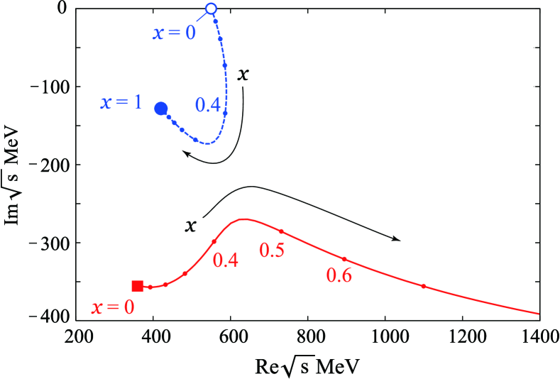
Figure 5: (color online) Trajectories of the poles of $\hat{D}$ by changing the parameter $x$. The open circle ($\circ$) indicates the mass of the elementary $\sigma$ meson, $m_{0}$, and the solid square ($\blacksquare$) the pole position of the composite $\sigma$ generated by the four-pion interaction only. The solid circle (•) indicates the pole position of the physical state at $x=1$.

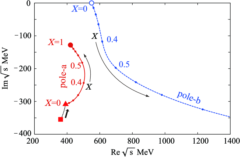
Figure 6: (color online) Trajectories of the poles of $\hat{D}$ by changing the mixing parameter $X$. The open circle ($\circ$) indicates the mass of the elementary $\sigma$ meson, $m_{0}$, the solid square ($\blacksquare$) the pole position of the composite $\sigma$ generated by the four-pion interaction only. The solid triangle ($\blacktriangle$) indicates the pole position of the composite $\sigma$ meson developed by the four-pion interaction and the $\sigma$-exchange in $t$- and $u$-channels. The solid circle (•) indicates the pole position of the physical state at $X=1$. The thick arrow shows the shift of the composite pole position by adding the $\sigma$-exchange term as explained in text.

IV.1.2 Parameterization-(II)

Next, to investigate the mixing properties in the two-level problem, we introduce the mixing parameter $X$ in front of the $v_{\rm pole}$ as,

$$v(s;X)=v_{\rm con}(s)+Xv_{\rm pole}(s)$$ (35)

which controls the mixing strength of the elementary $\sigma$ meson to the amplitude. We call this “parameterization-(II)”. Unlike the case (I), the $\sigma$-exchange in $t$- and $u$-channels is already included in $v_{\rm con}$. At $X=0$, we find a pole at $\sqrt{s}=390.7-308.4i$ MeV (solid triangle in Fig. 6), which we have called the composite $\sigma$-pole in this article. In contrast to this pole, we refer to the pole generated by the four-pion interaction only (solid square in Fig. 6) as naive-composite $\sigma$ to distinguish them. We find that the $\sigma$-exchange contribution shifts the composite pole position (as shown by the thick arrow in the figure), but its contribution is small. When the mixing is turned on, unlike the case (I), “level-repulsion & width-crossing” takes place. The pole starting from the composite $\sigma$ moves closer to the real axis (we refer to it as “pole-a”) and becomes the physical state at $X=1$, while that from the elementary $\sigma$ (“pole-b”) goes far away from the real axis and finally disappear exactly at $X=1$.

From the above analysis, we observe that the pole-flow is not a unique one but depends very much on the choice of the flow parameter, $x$ or $X$. This further indicates that the nature of the physical pole at $x$ or $X=1$ does not reflect that of the pole at the original point, $x$ or $X=0$, connected by the flow.

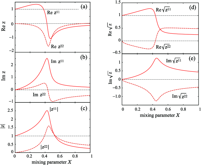
Figure 7: (color online) Residues $z^{11}$ and $z^{22}$ of the full propagator $D^{11}$ and $D^{22}$ at the pole-a shown in Fig. 6 as functions of the mixing parameter $X$. (a) The real parts of the residues, (b) those of the imaginary parts, (c) the modulus of the residues, (d) the real parts of the square-root of the residues and (e) those of the imaginary parts are shown, respectively.

IV.2 residues and the nature of the resonance

To study the mixing nature of the poles, we evaluate the residues $z^{11}$ and $z^{22}$ of pole-a (red solid line in Fig. 6) with parameterization-(II). In Fig. 7 we show the residues as functions of the mixing parameter $X$. First, recall that at $X=0$ the pole-a is purely the composite $\sigma$ meson ($z^{11}=1$ and $z^{22}=0$) as we expected.

Around $X\sim 0.4$ – $0.5$, $|z^{11}|$ and $|z^{22}|$ take the maximum value larger than 1, where in complex-energy plane pole-a and pole-b come closest to each other. This behavior of the residues looks like “resonance-shape”. For example, the line shape of the real (imaginary) part of $z^{11}$ is similar to the resonance shape of the real (imaginary) part of a scattering amplitude. In fact, we can understand this behavior by explicitly writing down the propagator, for example, $D^{22}$. Let $m_{a}^{*}(X)$ and $m_{b}^{*}(X)$ be the two pole values of the full propagator as functions of $X$, then we have

$$D^{22}(s;X)=\frac{\zeta(s)(s-s_{p})}{(s-m_{a}^{*2}(X))(s-m_{b}^{*2}(X))}\ ,$$ (36)

$$z_{a}^{22}\equiv\left.{\rm Res}D^{22}\right|_{s=m_{a}^{*2}}=\frac{\zeta(m_{a}^{*2})(m_{a}^{*2}-s_{p})}{m_{a}^{*2}(X)-m_{b}^{*2}(X)}$$ (37)

where $\zeta(s)$ is assumed to be $\zeta(m_{a}^{*2})\neq 0,\neq\infty$ (and in fact it is the case). Clearly the residue $|z_{a}^{22}|$ has a maximum value as a function of $X$ when $m_{a}^{*}$ approaches nearest $m_{b}^{*}$. Such a phenomenon, however, does not occur in a classical two-level problem. There only a level-repulsion takes place and residues do not exceed 1. The case study for possible values of residues are given in Appendix B.

At the physical point $X=1$, the real part of $z^{22}$ is almost zero and that of $z^{11}$ has a finite value as seen in Fig. 7(a). It seems that the physical $\sigma$ state is purely composite and has no component of the elementary $\sigma$ meson. However, there is a finite component in the physical state or, to be more precise, there must be a finite contribution from elementary $\sigma$ to the amplitude, because Im $z^{22}$ is not zero as shown in Fig. 7(b), and it influences the amplitude Eq. (32) as well as the real part does. Therefore we show the modulus of the residues as functions of the mixing parameter $X$ in Fig. 7(c) as a measure for the contributions from the basis states to the amplitude. For smaller $X$ the composite $\sigma$ dominates the physical state ($|z^{11}|>|z^{22}|$), at $X\sim 0.5$ their contributions become comparable ($|z^{11}|\sim|z^{22}|$), and at the physical point $X=1$ the component of elementary $\sigma$ meson becomes larger than that of the composite $\sigma$ meson ($|z^{11}|<|z^{22}|)$.

In Figs. 7(d) and (e), we show the square-root of the residues $\sqrt{z^{ii}}$ as functions of the mixing parameter $X$ because it appears in the form of square-root in Eq. (32). We find that the strength of the imaginary parts of the square-root of the residues, Im$\sqrt{z^{11}}$ and Im$\sqrt{z^{22}}$, are quite similar for all $X$, which allows us to forget about the imaginary part when discussing dominant component. As for the real part, we can clearly see again that the strengths of Re$\sqrt{z^{11}}$ and Re$\sqrt{z^{11}}$ become similar at $X\sim 0.5$, and the contribution from the elementary $\sigma$ becomes larger than that of the composite $\sigma$ at the physical point $X=1$. As a result, when the mass of the elementary $\sigma$ meson $m_{0}=550$ MeV is employed, the elementary nature becomes predominant in the physical $\sigma$ meson. In a later section, we will study the $m_{0}$ dependence of the results.

IV.3 a fate of pole-b and the number of poles

Now, let us go back to the discussion of properties of pole-b.

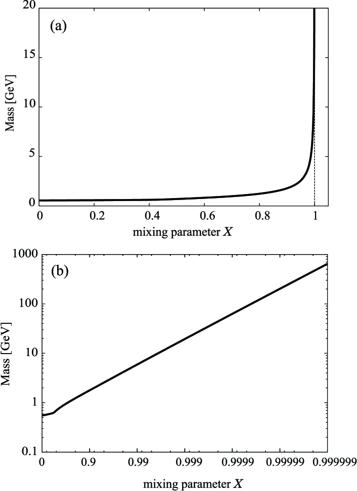
Figure 8: Mass of pole-b as functions of mixing parameter $X$, defined by the real part of the pole position in complex-energy plane, plotted (a) in linear plot and (b) in double logarithmic plot.

As shown in Figs. 5 and 6, we have two poles at finite $x$ and $X$, but one of these poles goes far away from the energy region of interest as $x$ and/or $X$ is increased. In Fig. 8, as an example, we show the real part of the pole position of pole-b with parameterization-(II) (shown in Fig. 6) as a function of the mixing parameter $X$. We find that pole-b goes to infinity in the limit $X=1$. This behavior can be understood by looking at the total potential $v_{\rm con}+v_{\rm pole}$. For large $s$, where pole-b is expected to locate, the total potential is expanded at $1/s\rightarrow 0$ as

$$v_{\rm con}+Xv_{\rm pole}\xrightarrow[\text{large }s]{} - \frac{3(1-X)}{f_{\pi}^{2}}s$$ (38)

$$+ \frac{1}{f_{\pi}^{2}}\left\{m_{\pi}^{2}(1-6X)+m_{0}^{2}(3X+2)\right\}$$

$$+ {\cal O}\left(\frac{1}{s}\right).$$

The first term is the leading and only one for the attraction, but it disappears at $X=1$, and so does pole-b.

This can be seen in a better manner by using parameterization-(I). The first term of Eq. (34) yields the composite $\sigma$ meson and the second term introduces the elementary $\sigma$ meson, which can be rewritten algebraically as

$$A(s) = -\frac{1}{f_{\pi}^{2}}(s-m_{\pi}^{2})+x\frac{1}{f_{\pi}^{2}}\frac{(s-m_{\pi}^{2})^{2}}{s-m_{0}^{2}}$$

$$= \frac{1}{f_{\pi}^{2}}\frac{(s-m_{\pi}^{2})(m_{0}^{2}-m_{\pi}^{2})}{s-m_{0}^{2}}+(1-x)\frac{1}{f_{\pi}^{2}}\frac{(s-m_{\pi}^{2})^{2}}{s-m_{0}^{2}}.$$

We may interpret the second line as that there are two different “seeds” having the same mass $m_{0}$ with different coupling strengths. Obviously, the second seed vanishes at $x=1$, leaving only one seed.

This can be understood physically if we consider that the function $A(s)$ with $x=1$ can be also expressed as

$$A(s)=\frac{1}{f_{\pi}^{2}}(m_{0}^{2}-m_{\pi}^{2})+\frac{1}{f_{\pi}^{2}}(m_{0}^{2}-m_{\pi}^{2})^{2}\frac{1}{s-m_{0}^{2}}.$$ (40)

This form is identical to what one obtains in the linear representation of the sigma model, where the first term expresses the repulsive four-pion interaction giving no composite $\sigma$ state dynamically. There, the unitarized amplitude has the only one pole associated with the second term corresponding to the elementary $\sigma$ meson acquiring a finite width through the coupling to the two-pion channel. Because of the representation independence of the sigma model Donoghue et al. (1992), we should have only one pole also in the nonlinear representation. In this case the elementary $\sigma$ pole is considered to behave like a counter term for the composite $\sigma$ pole without introducing a second pole.

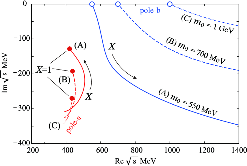
Figure 9: (color online) Trajectories of the poles of $\hat{D}$ by changing the mixing parameter $X$ for different mass of the elementary $\sigma$ (A) $m_{0}=550$ MeV (solid lines), (B) $m_{0}=700$ MeV (dashed lines), and (C) $m_{0}=1$ GeV (dotted lines). The open circles indicate the mass of the elementary $\sigma$ meson, $m_{0}$, and the solid circles indicate the pole position of the physical state at $X=1$ for each $m_{0}$ case.

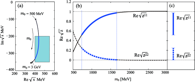
Figure 10: (color online) (a) Trajectory of the poles of $\hat{D}$ at $X=1$ by changing the mass of the elementary $\sigma$, $m_{0}$. The solid square indicates the pole position of the naive-composite $\sigma$ meson, which is also obtained in $m_{0}\rightarrow\infty$ limit. The (blue) hatched area denotes the energy range of the experimental value of the $\sigma$ mass $m_{\sigma}=400$ – 550 MeV and width $\Gamma_{\sigma}=400$ – 700 MeV in PDG. Beringer et al. (2012). (b) The real parts of the square-root of the residues at the resulting pole at $X=1$ as functions of $m_{0}$. The area between two vertical dashed-lines corresponds to the case in which the corresponding pole are within the errorbars of the PDG value Beringer et al. (2012). (c) The possible range of Re$\sqrt{z^{11}}$ and Re$\sqrt{z^{22}}$ when the resulting pole position is within errorbars of PDG value Beringer et al. (2012).

Such a situation occurs only at $x=1$, implying that the number of poles depends on the coupling strength of $\sigma\pi\pi$. In fact, we have found two poles in our previous study for the $a_{1}(1260)$ axial vector meson Nagahiro et al. (2011). There the interaction kernel for the $\pi\rho$ scattering is given by the Weinberg-Tomozawa interaction for $\pi\rho$ system and the $a_{1}$-pole term Bando et al. (1988); Nagahiro et al. (2011),

$$V_{WT}=-\frac{1}{4f_{\pi}^{2}}\left\{3s-2(m_{\rho}^{2}+m_{\pi}^{2})-\frac{1}{s}(m_{\rho}^{2}-m_{\pi}^{2})^{2}\right\},$$ (41)

$$V_{a_{1}\text{-pole}}=\frac{1}{2f_{\pi}^{2}}(s-m_{\rho}^{2})^{2}\frac{1}{s-m_{a_{1}}^{2}}.$$ (42)

We have found two poles for all $x$ even at $x=1$ where $x$ is introduced as $V_{\rm total}=V_{WT}+xV_{a_{1}\text{-pole}}$. Indeed, the leading term of the total potential $V_{\rm total}$ remains for large $s$ at $x=1$,

$$V_{WT}+V_{a_{1}\text{-pole}}\xrightarrow[\text{large }s]{}-\frac{s}{4f_{\pi}^{2}}+\frac{m_{a_{1}}^{2}-m_{\rho}^{2}+m_{\pi}^{2}}{2f_{\pi}^{2}}+{\cal O}\left(\frac{1}{s}\right).$$ (43)

We find that, however, the pole-b in Ref. Nagahiro et al. (2011) goes to infinity as well at $x=3/2$, where the leading term of the total potential vanishes,

$$V_{WT}+\frac{3}{2}V_{a_{1}\text{-pole}}\xrightarrow[\text{large }s]{}\frac{3m_{a_{1}}^{2}-4m_{\rho}^{2}+2m_{\pi}^{2}}{4f_{\pi}^{2}}+{\cal O}\left(\frac{1}{s}\right)\ \ .$$ (44)

So we conclude that, although we can define two basis states as independent degrees of freedom, we do not necessarily have two resulting states. Incidentally, it may be interesting to note that the condition as Eqs. (38) or (44) is nothing but the unitarity condition for the tree-level amplitude.

IV.4 $m_{0}$ dependence

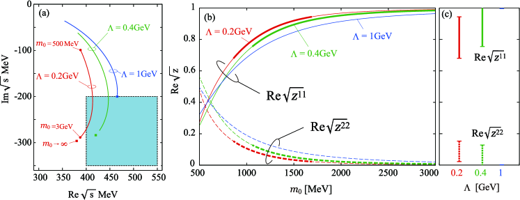
Figure 11: (color online) (a) Trajectories of the poles of $\hat{D}$ at $X=1$ by changing the mass of the elementary $\sigma$, $m_{0}$, for different cut-off values $\Lambda$. The solid squares indicate the pole positions of the naive-composite $\sigma$ meson, which are also obtained in $m_{0}\rightarrow\infty$ limit. The (blue) hatched area denotes the energy range of experimental value of the $\sigma$ mass $m_{\sigma}=400$ – 550 MeV and width $\Gamma_{\sigma}=400$ – 700 MeV in PDG Beringer et al. (2012). (b) The real parts of the square-root of the residues at the poles at $X=1$ as functions of $m_{0}$ for different $\Lambda$. The thick lines corresponds to the case in which corresponding poles are within errorbars of the PDG value Beringer et al. (2012). (c) The possible range of Re$\sqrt{z^{11}}$ and Re$\sqrt{z^{22}}$ for different $\Lambda$ when the resulting pole position is within errorbars of the PDG value Beringer et al. (2012).

Next, we discuss the dependence of the resulting state on the mass of the elementary $\sigma$, $m_{0}$. In Fig. 9, we show the pole-flow by changing the mixing parameter $X$ for different $m_{0}$ values, 550 MeV, 700 MeV, and 1 GeV. As $m_{0}$ is increased, the range of the flow of pole-a becomes narrower, and in the limit $m_{0}\rightarrow\infty$ the pole-a stays at a single point while changing the parameter $X$. In contrast, the flow of pole-b is getting further away from pole-a and disappears at $X=1$ in any case. In Fig. 10(a), we show the trajectories of the resulting pole at $X=1$ by changing $m_{0}$. We can see that, as $m_{0}$ is increased, the resulting pole approaches the naive-composite $\sigma$ pole (solid square). The residues shown in Fig. 10(b) also indicate that the nature of the physical pole approaches the naive-composite one in the heavy $m_{0}$ limit,

$$\sqrt{z^{11}}\xrightarrow[m_{0}\rightarrow\infty]{}1\ ,\sqrt{z^{22}}\xrightarrow[m_{0}\rightarrow\infty]{}0\ .$$ (45)

In other words, the wave function renormalization of the elementary $\sigma$ becomes zero in the limit $m_{0}\rightarrow\infty$. Weinberg (1965).

In Fig. 10(a), we show the region of the experimental values of the mass and width of the $\sigma$ meson shown in Particle Data Group (PDG) Beringer et al. (2012). We find that, to reproduce the data within the present model, we need a rather large mass of the the elementary $\sigma$ meson, $m_{0}\sim 730$ – 1660 MeV, when the natural value of the subtraction constant is used, although the elementary component is always smaller than that of the composite one (${\rm Re}\sqrt{z^{11}}>{\rm Re}\sqrt{z^{22}}$) as shown in Figs. 10(b) and (c). The values of residues are obtained as ${\rm Re}\sqrt{z^{11}}\sim 0.52$ – 0.98 and ${\rm Re}\sqrt{z^{22}}\sim 0.25$ – $2.0\times 10^{-4}$, respectively.

IV.5 cut-off dependence

$\Lambda$	naive-composite pole	$m_{0}$
${\rm[MeV]}$	[MeV]	[MeV]	$\sqrt{z^{11}}$	$\sqrt{z^{22}}$	$|z^{22}|$
200	$380-296i$	860 – 1690	$0.68+0.34i$ – $0.94+0.16i$	$0.15-0.25i$ – $0.022-0.091i$	0.085 – $8.8\times 10^{-3}$
300	$400-293i$	930 $<$	$0.71+0.32i$	$0.15-0.24i$	$7.8\times 10^{-2}<$
400	$420-284i$	1060$<$	$0.76+0.29i$	$0.13-0.20i$	$5.6\times 10^{-2}<$
500	$436-270i$	$1220<$	$0.80+0.24i$	$0.10-0.16i$	$3.7\times 10^{-2}<$
600	$448-255i$	$1430<$	$0.85+0.19i$	$0.080-0.12i$	$2.1\times 10^{-2}<$
700	$456-240i$	$1710<$	$0.90+0.15i$	$0.058-0.088i$	$1.1\times 10^{-2}<$
800	$461-226i$	$2160<$	$0.93+0.10i$	$0.036-0.057i$	$4.6\times 10^{-3}<$
900	$464-213i$	$3060<$	$0.97+0.05i$	$0.018-0.029i$	$1.2\times 10^{-3}<$
1000	$465-201i$	$9240<$	$0.997+0.0058i$	$0.002-0.003i$	$1.4\times 10^{-5}<$

Table 2: Critical values of $m_{0}$ for which the resulting pole is within the errorbars of the PDG value Beringer et al. (2012) $m_{\sigma}=400$ – $550$ MeV and $\Gamma_{\sigma}=400$ – 700 MeV for different $\Lambda$ in the third column. The corresponding residues are also shown in the following columns. For $\Lambda=200$ MeV case, there is an upper limit of $m_{0}$ as well as a lower limit, while there is only the lower limit for $\Lambda=300$ MeV – 1 GeV. In the second column, the naive-composite pole position (obtained with $m_{0}\rightarrow\infty$) is shown. If the naive-composite pole is within the errorbars of the PDG value, it means that there is no upper limit for $m_{0}$.

So far, we employed the natural value for the subtraction constant $a(\mu)$ in the dimensional regularization scheme Hyodo et al. (2008, 2010). As discussed in Ref. Hyodo et al. (2008), introducing the subtraction constant different from the natural value is equivalent to the introduction of the CDD pole term. Generally, the CDD pole can be expressed as an elementary particle in a Lagrangian, which is regarded as a counter term of the renormalization. The use of the different subtraction constant (renormalization condition) is therefore absorbed into the mass of the elementary particle. At this point, it should be emphasized that the resulting amplitude $t$ does not change. However, by changing the subtraction constant and accordingly the mass of the CDD pole (elementary particle), the mixing ratio may change, since the wave function renormalization $z^{ii}$ depends on the mass of the elementary particle as shown in the previous section. In other words, the theory alone cannot determine the mixing nature of the resonance. Hence we need an extra condition for them, in accordance with which the mixing ratio is determined.

In the present analysis, we have determined the extra condition by employing the natural value for the subtraction constant. This corresponds to the use of the cut-off $\Lambda\sim 180$ MeV when the three-dimensional cut-off scheme is employed for the loop function. This value, however, seems somewhat too small as compared to the typical hadronic scale $\sim 1$ GeV. To make physical insight clearer, in what follows we consider the three-dimensional cut-off scheme with different values of $\Lambda$.

In Fig. 11(a), we show the trajectory of the resulting poles by changing $m_{0}$ when $\Lambda=200$ MeV is employed (red line in the figure). The flow is similar to that of the natural value case shown in Fig. 10(a). In Fig. 11(a) we also show the trajectories for different cut-off values $\Lambda=400$ MeV and 1 GeV. We note that the trajectories do not overlap despite the above discussion that the change of the cut-off (regularization parameter) value is equivalent to the change of $m_{0}$. One of the reason is that the three-dimensional cut-off used here breaks covariance of the theory. Then the difference of the loop function coming from the different three-dimensional cut-off $\Lambda$ cannot be absorbed in the mass of the elementary particle. Second reason, which is indeed the main source of the difference, is found in the unitarization procedure employed in this work. Although the equivalence holds only when summing up the diagrams including the $s$-pole in the direction of $s$-channel, we sum up the $t$- and $u$-exchange diagrams as well in the direction of $s$-channel. Therefore, the mass of the “exchanged $\sigma$ meson” cannot compensate for the regularization parameter. But still the difference coming from these reasons is not large as shown in Figs. 11(a) and (b).

Now we observe that the resulting pole tends to approach the real axis as $\Lambda$ increases from 200 MeV to 1 GeV. This behavior resembles the flow of pole-a when $m_{0}$ is decreased. To put it the other way around, in the case of large cut-off $\Lambda$ we need to have heavier mass of the elementary $\sigma$ to reproduce the large width of the $\sigma$ meson of the PDG value Beringer et al. (2012). As summarized in Table 2, the component of the elementary $\sigma$ in the resulting state becomes smaller for larger cut-off.

It is interesting to see that, for cut-off values of hadronic scale, the mass of the elementary $\sigma$ turns out to be rather heavy, and the mixing ratio of the elementary component is quite small. For instance, for $\Lambda=400$ MeV the mass of the elementary $\sigma$ is at least 1 GeV. When $\Lambda=1$ GeV is employed, the mass of the elementary $\sigma$ should be larger than 9 GeV and the resulting pole is almost pure composite $\sigma$ meson, Re$\sqrt{z^{11}}\sim 1$ and Re$\sqrt{z^{22}}\sim 0$.

V summary

The mixing nature of the scalar resonance $\sigma$ consisting of the $\pi\pi$ composite $\sigma$ and elementary $\sigma$ has been investigated within the sigma model in the nonlinear representation. We have shown that the unitarized scattering amplitude can be expressed in the form of the two-level problem. The mixing strengths of the composite and elementary $\sigma$ mesons have been evaluated by means of the residues of the full propagators of the composite and elementary $\sigma$ mesons.

The major findings of this study are summarized as follows:

• A rather heavy mass of the elementary $\sigma$ meson at least $m_{0}\gtrsim 1$ GeV is preferred, if experimental data from PDG is to be reproduced.

• The elementary $\sigma$ component is small and the $\pi\pi$ composite state dominates the physical $\sigma$.

We also have found the following interesting properties as the two-level problem of composite and elementary particles:

• Even if we have two basis states of the composite and elementary particles, it happens that only one state remains, depending on the strength of the interactions.

• The sigma model represented in the nonlinear base is described by the two basis states, which generates the only one $\sigma$ state.

Here we would like to emphasize that whether a physical particle is more elementary or composite like depends on the model Lagrangian and on how we define the two bases. In the sigma model in the nonlinear representation, the resulting physical $\sigma$ can be more composite like than the elementary like. We will further discuss this issue elsewhere Nagahiro and Hosaka .

Appendix A the scattering amplitude in the form of the two-level problem

Here we show the derivation of the scattering amplitude in the form of Eq. (23). To this end, we first define a function $\omega$ by

$$v_{\rm con}=g_{R}\omega g_{R}\ ,$$ (46)

where $g_{R}$ is the vertex function introduced in Eq. (22). By expressing $v_{\rm pole}$ in Eq. (19) similarly as

$$v_{\rm pole}=gD_{\sigma}g\ ,$$ (47)

we rewrite the potential terms in a matrix form as,

$$v_{\rm con}+v_{\rm pole} = g_{R}\omega g_{R}+gD_{\sigma}g$$ (48)

$$= (g_{R},g)\begin{pmatrix}\omega&0\\ 0&D_{\sigma}\end{pmatrix}\begin{pmatrix}g_{R}\\ g\end{pmatrix}.$$

Here $g$ is the coupling of $\sigma\pi\pi$ as $g^{2}=3(s-m_{\pi}^{2})^{2}/f_{\pi}^{2}$ and $D_{\sigma}$ the free propagator of the elementary $\sigma$ meson $D_{\sigma}^{-1}=s-m_{0}^{2}$. Then the full amplitude can be rewritten as

$$t = (v_{\rm con}+v_{\rm pole})+(v_{\rm con}+v_{\rm pole})G(v_{\rm con}+v_{\rm pole})+\cdots$$ (49)

$$= (g_{R},g)\begin{pmatrix}\omega&0\\ 0&D_{\sigma}\end{pmatrix}\begin{pmatrix}g_{R}\\ g\end{pmatrix}+(g_{R},g)\begin{pmatrix}\omega&0\\ 0&D_{\sigma}\end{pmatrix}\begin{pmatrix}g_{R}\\ g\end{pmatrix}G(g_{R},g)\begin{pmatrix}\omega&0\\ 0&D_{\sigma}\end{pmatrix}\begin{pmatrix}g_{R}\\ g\end{pmatrix}+\cdots$$

$$= (g_{R},g)\left[\begin{pmatrix}\omega&0\\ 0&D_{\sigma}\end{pmatrix}+\begin{pmatrix}\omega&0\\ 0&D_{\sigma}\end{pmatrix}\begin{pmatrix}g_{R}Gg_{R}&g_{R}Gg\\ gGg_{R}&gGg\end{pmatrix}\begin{pmatrix}\omega&0\\ 0&D_{\sigma}\end{pmatrix}+\cdots\right]\begin{pmatrix}g_{R}\\ g\end{pmatrix}$$

$$= (g_{R},g)\frac{1}{\begin{pmatrix}\omega&0\\ 0&D_{\sigma}\end{pmatrix}^{-1}-\begin{pmatrix}g_{R}Gg_{R}&g_{R}Gg\\ gGg_{R}&gGg\end{pmatrix}}\begin{pmatrix}g_{R}\\ g\end{pmatrix}$$ (50)

$$= (g_{R},g)\frac{1}{\begin{pmatrix}\omega^{-1}-g_{R}Gg_{R}&0\\ 0&D_{\sigma}^{-1}\end{pmatrix}-\begin{pmatrix}0&g_{R}Gg\\ gGg_{R}&gGg\end{pmatrix}}\begin{pmatrix}g_{R}\\ g\end{pmatrix}$$ (51)

$$= (g_{R},g)\frac{1}{\begin{pmatrix}s-s_{p}&0\\ 0&s-m_{0}^{2}\end{pmatrix}-\begin{pmatrix}0&g_{R}Gg\\ gGg_{R}&gGg\end{pmatrix}}\begin{pmatrix}g_{R}\\ g\end{pmatrix}\ ,$$ (52)

where in the last line we use the relation

$$\omega^{-1}-g_{R}Gg_{R}=g_{R}^{2}(v_{\rm con}^{-1}-G) = g_{R}^{2}t_{\rm composite}^{-1}$$ (53)

$$= s-s_{p}\ \ .$$

Finally we obtain the full scattering amplitude in a matrix form as

$$t=(g_{R},g)\frac{1}{\hat{D}_{0}^{-1}-\hat{\Sigma}}\begin{pmatrix}g_{R}\\ g\end{pmatrix}\ ,$$ (54)

where

$$\hat{D}_{0}^{-1}=\begin{pmatrix}s-s_{p}&0\\ 0&s-m_{0}^{2}\end{pmatrix},\ \hat{\Sigma}=\begin{pmatrix}0&g_{R}Gg\\ gGg_{R}&gGg\end{pmatrix}\ .$$ (55)

Appendix B possible values of residues

As discussed in Sec. IV, we have observed that the wave function renormalization constants $z^{ii}$ take a maximum value at a finite mixing parameter $X$. Such a phenomenon does not occur in a classical two-level problem. In this appendix, we discuss the possible values for the wave function renormalization in the two-level problem.

Let us consider a simple form of two-level Hamiltonian,

$$\hat{H}=\begin{pmatrix}s-m_{1}^{2}&0\\ 0&s-m_{2}^{2}\end{pmatrix}-\begin{pmatrix}0&v\\ v&0\end{pmatrix}$$ (56)

where $m_{1}$ and $m_{2}$ denote the masses of two basis states and $v$ a mixing potential between them. When $m_{1}$, $m_{2}$ and $v$ are real and energy-independent, the mass difference between the two resulting states becomes larger which is so-called the level-repulsion. In this case, the wave function renormalizations $z^{ii}$ for two states should take a value

$$0<z^{11}(z^{22})<1\ ,$$ (57)

and satisfy the sum rule

$$z^{11}+z^{22}=1\ .$$ (58)

When the mixing potential is complex value but energy-independent, the sum rule is still satisfied as

$${\rm Re}\,z^{11}+{\rm Re}\,z^{22}=1,\ \ {\rm Im}\,z^{11}+{\rm Im}\,z^{22}=0.$$ (59)

This sum rule is held as far as the potential is energy-independent. In such a case two levels can come closer and Re $z^{11}$ and/or Re $z^{22}$ can take a value larger than 1 or even becomes negative.

In the present case of the $\sigma$ system, the sum rule is also broken as

$$z^{11}+z^{22}\neq 1\ .$$ (60)

This is due to the energy-dependence of the mixing potential (self-energy) $\hat{\Sigma}$ in Eq. (24). One of origins of the energy dependence comes from the fact that the self-energy $\hat{\Sigma}$ includes the effect of the coupling to the two pion continuum. By eliminating the latter, $\hat{\Sigma}$ becomes energy dependent. This situation is the same that the wave function renormalization of one-particle propagator takes a different value than 1 due to one-loop corrections. Another source is the energy-dependence of the couplings $g(s)$ and $g_{R}(s)$. In fact, this energy dependence strongly influences the value of $z^{ii}$ when the poles flow over the wide energy range in complex-energy plane.

References

- Beringer et al. (2012) J. Beringer et al. (Particle Data Group), Phys. Rev. D 86, 010001 (2012).
- Basdevant and Lee (1970) J. L. Basdevant and B. W. Lee, Phys. Rev. D 2, 1680 (1970).
- Achasov and Shestakov (1994) N. N. Achasov and G. N. Shestakov, Phys. Rev. D 49, 5779 (1994).
- Törnqvist and Roos (1996) N. A. Törnqvist and M. Roos, Phys. Rev. Lett. 76, 1575 (1996).
- Harada et al. (1996) M. Harada, F. Sannino, and J. Schechter, Phys. Rev. D 54, 1991 (1996).
- Harada et al. (1997) M. Harada, F. Sannino, and J. Schechter, Phys. Rev. Lett. 78, 1603 (1997).
- Oller and Oset (1997) J. Oller and E. Oset, Nucl.Phys. A620, 438 (1997).
- Igi and Hikasa (1999) K. Igi and K.-i. Hikasa, Phys. Rev. D 59, 034005 (1999).
- Oller et al. (1999) J. A. Oller, E. Oset, and J. R. Pelaez, Phys. Rev. D59, 074001 (1999).
- Hyodo et al. (2010) T. Hyodo, D. Jido, and T. Kunihiro, Nucl. Phys. A848, 341 (2010).
- Nagahiro et al. (2011) H. Nagahiro, K. Nawa, S. Ozaki, D. Jido, and A. Hosaka, Phys.Rev. D83, 111504 (2011).
- Bando et al. (1988) M. Bando, T. Kugo, and K. Yamawaki, Phys. Rept. 164, 217 (1988).
- Roca et al. (2005) L. Roca, E. Oset, and J. Singh, Phys. Rev. D72, 014002 (2005).
- Nagahiro et al. (2009) H. Nagahiro, L. Roca, A. Hosaka, and E. Oset, Phys. Rev. D79, 014015 (2009).
- Donoghue et al. (1992) J. F. Donoghue, E. Golowich, and B. R. Holstein, Dynamics of the Standard Model (Cambridge University Press, Cambridge, 1992).
- Hyodo et al. (2008) T. Hyodo, D. Jido, and A. Hosaka, Phys. Rev. C78, 025203 (2008).
- Weinberg (1965) S. Weinberg, Phys. Rev. 137, B672 (1965).
- Lurie and Macfarlane (1964) D. Lurie and A. J. Macfarlane, Phys. Rev. 136, B816 (1964).
- Lurie (1968) D. Lurie, Particle and Fields (Interscience Publishers, New York, 1968).
- Hyodo et al. (2012) T. Hyodo, D. Jido, and A. Hosaka, Phys. Rev. C 85, 015201 (2012).
- (21) H. Nagahiro and A. Hosaka, in preparaion.
- Nawa et al. (2011) K. Nawa, S. Ozaki, H. Nagahiro, D. Jido, and A. Hosaka, (2011), arXiv:1109.0426 [hep-ph] .
- Sakai and Sugimoto (2005a) T. Sakai and S. Sugimoto, Prog. Theor. Phys. 113, 843 (2005a).
- Sakai and Sugimoto (2005b) T. Sakai and S. Sugimoto, Prog. Theor. Phys. 114, 1083 (2005b).