Spectroscopic parameters and decays of the resonance $Z_{b}(10610)$

Abstract

The resonance $Z_{b}(10610)$ is investigated as the diquark-antidiquark $Z_{b}=[bu][\overline{b}\overline{d}]$ state with spin-parity $J^{P}=1^{+}$. The mass and current coupling of the resonance $Z_{b}(10610)$ are evaluated using QCD two-point sum rule and taking into account the vacuum condensates up to ten dimensions. We study the vertices $Z_{b}\Upsilon(nS)\pi\ (n=1,2,3)$ by applying the QCD light-cone sum rule to compute the corresponding strong couplings $g_{Z_{b}\Upsilon(nS)\pi}$ and widths of the decays $Z_{b}\to\Upsilon(nS)\pi$. We explore also the vertices $Z_{b}h_{b}(mP)\pi\ (m=1,2)$ and calculate the couplings $g_{Z_{b}h_{b}(mP)\pi}$ and width of the decay channels $Z_{b}\to h_{b}(mP)\pi$. To this end, we calculate the mass and decay constants of the $h_{b}(1P)$ and $h_{b}(2P)$ mesons. The results obtained are compared with experimental data of the Belle Collaboration.

I Introduction

Discovery of the charged resonances which cannot be explained as $\bar{c}c$ or $\bar{b}b$ states has opened a new page in physics of exotic multi-quark systems. The first tetraquarks of this family are $Z^{\pm}(4430)$ states which were observed by the Belle Collaboration in $B$ meson decays $B\rightarrow K\psi^{\prime}\pi^{\pm}$ as resonances in the $\psi^{\prime}\pi^{\pm}$ invariant mass distributions Choi:2007wga . The mass and width of these states were repeatedly measured and refined. Recently, the LHCb Collaboration confirmed existence of the $Z^{-}(4430)$ structure in the decay $B^{0}\rightarrow K^{+}\psi^{\prime}\pi^{-}$ and unambiguously determined that its spin-parity is $J^{P}=1^{+}$ Aaij:2014jqa ; Aaij:2015zxa . They also measured the mass and width of $Z^{-}(4430)$ resonance and updated the existing experimental data. Two charmonium-like resonances $Z_{1}(4050)$ and $Z_{2}(4250)$ were discovered by the Belle Collaboration in the decay $\bar{B}^{0}\rightarrow K^{-}\pi^{+}\chi_{c1}$ which emerged as broad peaks in the $\chi_{c1}\pi$ invariant mass distribution Mizuk:2008me .

Famous members of the charged tetraquark family $Z_{c}^{\pm}(3900)$ were observed by the BESIII Collaboration in the process $e^{+}e^{-}\rightarrow J/\psi\pi^{+}\pi^{-}$ as resonances with $J^{P}=1^{+}$ in the $J/\psi\pi^{\pm}$ mass distribution Ablikim:2013mio . The charged state $Z_{c}(4020)$ was also found by the BESIII Collaboration in two different processes $e^{+}e^{-}\rightarrow h_{c}\pi^{+}\pi^{-}$ and $e^{+}e^{-}\rightarrow(D^{\star}\bar{D}^{\star})^{\pm}\pi^{\mp}$ (see, Refs. Ablikim:2013wzq ; Ablikim:2013emm ).

There is another charged state, namely $Z_{c}(4200)$ resonance which was detected and announced by Belle Chilikin:2014bkk . All aforementioned resonances belong to the class of the charmonium-like tetraquarks, and contain a $\bar{c}c$ pair and light quarks (antiquarks). They were mainly interpreted as diquark-antidiquark systems or bound states of $D$ and/or $D^{\star}$ mesons.

It is remarkable, that $b$-counterparts of the charmonium-like states, i.e. charged resonances composed of a $\bar{b}b$ pair and light quarks were found, as well. Thus, the Belle Collaboration discovered the resonances $Z_{b}(10610)$ and $Z_{b}(10650)$ (hereafter, $Z_{b}$ and $Z_{b}^{\prime}$, respectively) in the decays $\Upsilon(5S)\rightarrow\Upsilon(nS)\pi^{+}\pi^{-},\ n=1,2,3$ and $\Upsilon(5S)\rightarrow h_{b}(mP)\pi^{+}\pi^{-},\ m=1,2$ Belle:2011aa ; Garmash:2014dhx . These two states with favored spin-parity $J^{P}=1^{+}$ appear as resonances in the $\Upsilon(nS)\pi^{\pm}$ and $h_{b}(mP)\pi^{\pm}$ mass distributions. The masses of the $Z_{b}$ and $Z_{b}^{\prime}$ resonances are

$$m = (10607.2\pm 2.0)\ \mathrm{MeV},$$

$$m^{\prime} = (10652.2\pm 1.5)\ \mathrm{MeV},$$ (1)

respectively. The width of the $Z_{b}$ state averaged over five decay channels equals to $\Gamma=(18.4\pm 2.4)\ \mathrm{MeV}$, whereas the average width of $Z_{b}^{\prime}$ is $\Gamma^{\prime}=(11.5\pm 2.2)\ \mathrm{MeV}$. Recently, the dominant decay channel of $Z_{b}$ , namely $Z_{b}\rightarrow B^{+}\bar{B}^{\star 0}+\bar{B}^{0}B^{\star+}$ process was also observed Garmash:2015rfd . In this work fractions of different channels of $Z_{b}$ and $Z_{b}^{\prime}$ resonances were reported, as well. Further information on experimental status of the $Z_{b}$ and $Z_{b}^{\prime}$ states and other heavy exotic mesons and baryons can be found in Ref. Olsen:2017bmm .

An existence of hidden-bottom states, i.e. of the $Z_{b}$ resonances were foreseen before their experimental observation. Thus, in Ref. Karliner:2008rc authors suggested to look for the diquark-antidiquarks with $b\bar{b}u\bar{d}$ content as peaks in the invariant mass of $\Upsilon(1S)\pi$ and $\Upsilon(2S)\pi$ systems. The existence of the molecular state $B^{\star}\bar{B}$ was predicted in Ref. Liu:2008tn .

After discovery of the $Z_{b}$ resonances theoretical studies of the charged hidden-bottom states became more intensive and fruitful. In fact, works devoted to the structures and decay channels of the $Z_{b}$ states encompass all existing models and computational schemes suitable to study the multi-quark systems. Thus, in Refs. Bondar:2011ev ; Voloshin:2011qa the spectroscopic and decay properties of $Z_{b}$ and $Z_{b}^{\prime}$ were explored using the heavy quark symmetry by modeling them as $J=1$ $S$-wave molecular states $B^{\star}\bar{B}-B\bar{B}^{\star}$ and $B^{\star}\bar{B}^{\star}$, respectively. The existence of similar states with quantum numbers $0^{+},\ 1^{+},\ 2^{+}$ were predicted, as well. The diquark-antidiquark interpretation of the $Z_{b}$ states were proposed in Refs. Ali:2011ug ; Ali:2014dva . It was demonstrated that Belle results on the decays $\Upsilon(5S)\rightarrow\Upsilon(nS)\pi^{+}\pi^{-}$ and $\Upsilon(5S)\rightarrow h_{b}(mP)\pi^{+}\pi^{-}$ support $Z_{b}$ resonances as diquark-antidiquark states. This analysis is based on a scheme for the spin-spin quark interactions inside diquarks originally suggested and successfully used to explore hidden-charm resonances Maiani:2014 .

The $Z_{b}$ resonance was considered in Ref. Zhang:2011jja as a $B^{\star}\bar{B}$ molecular state, where its mass was computed in the context of QCD sum rule method. The prediction for the mass $m_{B^{\star}\bar{B}}=10.54\pm 0.22\ \mathrm{GeV}$ obtained there, allowed authors to conclude that $Z_{b}$ could be a $B^{\star}\bar{B}$ molecular state. The similar conclusions were also made in the framework of the chiral quark model. Indeed, in Ref. Yang:2011rp the $B\bar{B}^{\star}$ and $B^{\star}\bar{B}^{\star}$ bound states with $J^{PC}=1^{+-}$ were studied in the chiral quark model, and found as good candidates for $Z_{b}$ and $Z_{b}^{\prime}$ resonances. Moreover, existence of molecular states $B\bar{B}^{\star}$ with $J^{PC}=1^{++}$, and $B^{\star}\bar{B}^{\star}$ with $J^{PC}=0^{++},\ 2^{++}$ were predicted. Explorations performed using the one boson-exchange model also led to the molecular interpretations of the $Z_{b}$ and $Z_{b}^{\prime}$ resonances Sun:2011uh . However, analysis carried out in the framework of the Bete-Salpeter approach demonstrated that two heavy mesons can form an isospin singlet bound state but cannot form an isotriplet compound. Hence, the $Z_{b}$ resonance presumably is a diquark-antidiquark, but not a molecular state Ke:2012gm .

The both diquark-antidiquark and molecular pictures for internal organization of $Z_{b}$ and $Z_{b}^{\prime}$ within QCD sum rules method were examined in Ref. Cui:2011fj . In this work the authors constructed different interpolating currents with $I^{G}J^{P}=1^{+}1^{+}$ to explore the $Z_{b}$ and $Z_{b}^{\prime}$ states and evaluate their masses. Among alternative interpretations of the $Z_{b}$ states it is worth noting Refs. Bugg:2011jr and Danilkin:2011sh , where the peaks observed by the Belle Collaboration were explained as cusp and coupling channel effects, respectively.

Theoretical works that address problems of the $Z_{b}$ states are numerous (see, Refs. Chen:2011zv ; Chen:2011pv ; Cleven:2011gp ; Cleven:2013sq ; Mehen:2013mva ; Wang:2013daa ; Wang:2014gwa ; Dong:2012hc ; Chen:2015ata ; Kang:2016ezb ). Analysis of these and other investigations can be found in the recent review papers Esposito:2016noz ; Ali:2017jda .

As is seen, theoretical status of the resonances $Z_{b}$ and $Z_{b}^{\prime}$ remains controversial and deserves further and detailed explorations. In the present work we are going to calculate the spectroscopic parameters of $Z_{b}=[bu][\overline{b}\overline{d}]$ state by assuming that it is a tetraquark state with diquark-antidiquark structure and positive charge. We use QCD two-point sum rules to evaluate its mass and current coupling by taking into account vacuum condensates up to ten dimensions. We also investigate five observed decay channels of $Z_{b}$ resonance employing QCD sum rules on the light-cone. As a byproduct, we derive the mass and decay constant of $h_{b}(mP),\ m=1,2$ mesons.

This work has the following structure: In Sec. II we calculate the mass and current coupling of the $Z_{b}$ resonance. In Sec. III we analyze the decay channels $Z_{b}\rightarrow\Upsilon(nS)\pi,\ n=1,\ 2,\ 3$ and calculate their widths. Section IV is devoted to investigation of the decay modes $Z_{b}\rightarrow h_{b}(mP)\pi,\ m=1,\ 2$ and consists of two subsections. In the first subsection we calculate the mass and decay constant of the $h_{b}(1P)$ and $h_{b}(2P)$ mesons. To this end, we employ the two-point sum rule approach by including into analysis condensates up to eight dimensions. In the next subsection using parameters of the $h_{b}(mP)$ mesons we evaluate width of decays under investigation. The last section is reserved for analysis of the obtained results and discussion of possible interpretations of $Z_{b}$ resonance.

II Mass and current coupling of the $Z_{b}$ state: QCD two-point sum rule predictions

In this section we derive QCD sum rules to calculate the mass and current coupling of the $Z_{b}$ state by suggesting that it has a diquark-antidiquark structure with quantum numbers $I^{G}J^{P}=1^{+}1^{+}$.  To this end, we begin from the two-point correlation function

$$\Pi_{\mu\nu}(p)=i\int d^{4}xe^{ipx}\langle 0|\mathcal{T}\{J_{\mu}^{Z_{b}}(x)J_{\nu}^{Z_{b}{\dagger}}(0)\}|0\rangle,$$ (2)

where $J_{\mu}^{Z_{b}}(x)$ is the interpolating current for the $Z_{b}$ state with required quark content and quantum numbers.

It is possible to construct various currents to interpolate the $Z_{b}$ and $Z_{b}^{\prime}$ resonances. One of them is $[ub]_{S=0}[\overline{d}\overline{b}]_{S=1}-$ $[ub]_{S=1}[\overline{d}\overline{b}]_{S=0}$ type diquark-antidiquark current that is used to consider $Z_{b}$ state

$$J_{\mu}^{Z_{b}}(x)=\frac{i\epsilon\tilde{\epsilon}}{\sqrt{2}}\left\{\left[u_{a}^{T}(x)C\gamma_{5}b_{b}(x)\right]\left[\overline{d}_{d}(x)\gamma_{\mu}C\overline{b}_{e}^{T}(x)\right]\right.$$

$$\left.-\left[u_{a}^{T}(x)C\gamma_{\mu}b_{b}(x)\right]\left[\overline{d}_{d}(x)\gamma_{5}C\overline{b}_{e}^{T}(x)\right]\right\}.$$ (3)

The current for $Z_{b}^{\prime}$ can be defined in the form

$$J_{\mu}^{Z_{b}^{\prime}}(x)=\frac{\epsilon\tilde{\epsilon}}{\sqrt{2}}\varepsilon_{\mu\nu\alpha\beta}\left[u_{a}^{T}(x)C\gamma^{\nu}b_{b}(x)\right]$$

$$\times D^{\alpha}\left[\overline{d}_{d}(x)\gamma^{\beta}C\overline{b}_{e}^{T}(x)\right],$$ (4)

where $D^{\alpha}=\partial^{\alpha}-ig_{s}A^{\alpha}(x)$ Cui:2011fj . In Eqs. (3) and  (4) we have introduced the notations $\epsilon=\epsilon_{abc}$ and $\tilde{\epsilon}=\epsilon_{dec}$. In above expressions $a,b,c,d$ and $e$ are color indices, and $C$ is the charge conjugation matrix.

By choosing different currents to interpolate the $Z_{b}$ and $Z_{b}^{\prime}$ resonances one treats both of them as ground-state particles in corresponding sum rules. We also follow this approach and use the current $J_{\mu}^{Z_{b}}(x)$ to calculate the mass and current coupling of the $Z_{b}$ state. To find the QCD sum rules we first have to calculate the correlation function in terms of the physical degrees of freedom. To this end, we saturate $\Pi_{\mu\nu}(p)$ with a complete set of states with quantum numbers of $Z_{b}$ resonance and perform in Eq. (2) integration over $x$ to get

$$\Pi_{\mu\nu}^{\mathrm{Phys}}(p)=\frac{\langle 0|J_{\mu}^{Z_{b}}|Z_{b}(p)\rangle\langle Z_{b}(p)|J_{\nu}^{Z_{b}\dagger}|0\rangle}{m_{Z_{b}}^{2}-p^{2}}+...,$$

where $m_{Z_{b}}$ is the mass of the $Z_{b}$ state, and dots indicate contributions of higher resonances and continuum states. We define the current coupling $f_{Z_{b}}$ through the matrix element

$$\langle 0|J_{\mu}^{Z_{b}}|Z_{b}(p)\rangle=f_{Z_{b}}m_{Z_{b}}\varepsilon_{\mu},$$ (5)

with $\varepsilon_{\mu}$ being the polarization vector of $Z_{b}$ state. Then in terms of $m_{Z_{b}}$ and $f_{Z_{b}}$, the correlation function can be written in the following form

$$\Pi_{\mu\nu}^{\mathrm{Phys}}(p)=\frac{m_{Z_{b}}^{2}f_{Z_{b}}^{2}}{m_{Z_{b}}^{2}-p^{2}}\left(-g_{\mu\nu}+\frac{p_{\mu}p_{\nu}}{m_{Z_{b}}^{2}}\right)+\ldots$$ (6)

The Borel transformation applied to Eq. (6) gives

$$\mathcal{B}\Pi_{\mu\nu}^{\mathrm{Phys}}(p)=m_{Z_{b}}^{2}f_{Z_{b}}^{2}e^{-m_{Z_{b}}^{2}/M^{2}}\left(-g_{\mu\nu}+\frac{p_{\mu}p_{\nu}}{m_{Z_{b}}^{2}}\right)+\ldots$$ (7)

At the next stage we derive the theoretical expression for the correlation function $\Pi_{\mu\nu}^{\mathrm{QCD}}(p)$ in terms of the quark-gluon degrees of freedom. It can be determined using the interpolating current $J_{\mu}^{Z_{b}}$ and quark propagators. After contracting in Eq. (2) the $b$-quark and light quark fields we get

$$\Pi_{\mu\nu}^{\mathrm{QCD}}(p)=-\frac{i}{2}\int d^{4}xe^{ipx}\epsilon\tilde{\epsilon}\epsilon^{\prime}\tilde{\epsilon}^{\prime}\left\{\mathrm{Tr}\left[\gamma_{5}\widetilde{S}_{u}^{aa^{\prime}}(x)\right.\right.$$

$$\left.\times\gamma_{5}S_{b}^{bb^{\prime}}(x)\right]\mathrm{Tr}\left[\gamma_{\mu}\widetilde{S}_{b}^{e^{\prime}e}(-x)\gamma_{\nu}S_{d}^{d^{\prime}d}(-x)\right]$$

$$-\mathrm{Tr}\left[\gamma_{\mu}\widetilde{S}_{b}^{e^{\prime}e}(-x)\gamma_{5}S_{d}^{d^{\prime}d}(-x)\right]\mathrm{Tr}\left[\gamma_{\nu}\widetilde{S}_{u}^{aa^{\prime}}(x)\right.$$

$$\times\left.\gamma_{5}S_{b}^{bb^{\prime}}(x)\right]-\mathrm{Tr}\left[\gamma_{5}\widetilde{S}_{u}^{a^{\prime}a}(x)\gamma_{\mu}S_{b}^{b^{\prime}b}(x)\right]$$

$$\times\mathrm{Tr}\left[\gamma_{5}\widetilde{S}_{b}^{e^{\prime}e}(-x)\gamma_{\nu}S_{d}^{d^{\prime}d}(-x)\right]+\mathrm{Tr}\left[\gamma_{\nu}\widetilde{S}_{u}^{aa^{\prime}}(x)\right.$$

$$\left.\times\left.\gamma_{\mu}S_{b}^{bb^{\prime}}(x)\right]\mathrm{Tr}\left[\gamma_{5}\widetilde{S}_{b}^{e^{\prime}e}(-x)\gamma_{5}S_{d}^{d^{\prime}d}(-x)\right]\right\},$$ (8)

where

$$\widetilde{S}_{b(q)}^{ij}(x)=CS_{b(q)}^{ij\mathrm{T}}(x)C.$$

In expressions above $S_{q}^{ab}(x)$ and $S_{b}^{ab}(x)$ are the light $u,\ d\$ and heavy $b$-quark propagators, respectively. We choose the light quark propagator $S_{q}^{ab}(x)$ in the form

$$S_{q}^{ab}(x)=i\delta_{ab}\frac{\not{x}}{2\pi^{2}x^{4}}-\delta_{ab}\frac{m_{q}}{4\pi^{2}x^{2}}-\delta_{ab}\frac{\langle\overline{q}q\rangle}{12}$$

$$+i\delta_{ab}\frac{\not{x}m_{q}\langle\overline{q}q\rangle}{48}-\delta_{ab}\frac{x^{2}}{192}\langle\overline{q}g_{\mathrm{s}}\sigma Gq\rangle+i\delta_{ab}\frac{x^{2}\not{x}m_{q}}{1152}\langle\overline{q}g_{\mathrm{s}}\sigma Gq\rangle$$

$$-i\frac{g_{\mathrm{s}}G_{ab}^{\alpha\beta}}{32\pi^{2}x^{2}}\left[\not{x}{\sigma_{\alpha\beta}+\sigma_{\alpha\beta}}\not{x}\right]-i\delta_{ab}\frac{x^{2}\not{x}g_{\mathrm{s}}^{2}\langle\overline{q}q\rangle^{2}}{7776}$$

$$-\delta_{ab}\frac{x^{4}\langle\overline{q}q\rangle\langle g_{\mathrm{s}}^{2}G^{2}\rangle}{27648}+\ldots$$ (9)

For the $b$-quark propagator $S_{b}^{ab}(x)$ we employ the expression

$$S_{b}^{ab}(x)=i\int\frac{d^{4}k}{(2\pi)^{4}}e^{-ikx}\Bigg{\{}\frac{\delta_{ab}\left({\not{k}}+m_{b}\right)}{k^{2}-m_{b}^{2}}$$

$$-\frac{g_{s}G_{ab}^{\alpha\beta}}{4}\frac{\sigma_{\alpha\beta}\left({\not{k}}+m_{b}\right)+\left({\not{k}}+m_{b}\right)\sigma_{\alpha\beta}}{(k^{2}-m_{b}^{2})^{2}}$$

$$+\frac{g_{\mathrm{s}}^{2}G^{2}}{12}\delta_{ab}m_{b}\frac{k^{2}+m_{b}{\not{k}}}{(k^{2}-m_{b}^{2})^{4}}+\frac{g_{\mathrm{s}}^{3}G^{3}}{48}\delta_{ab}\frac{\left({\not{k}}+m_{b}\right)}{(k^{2}-m_{b}^{2})^{6}}$$

$$\times\left[{\not{k}}\left(k^{2}-3m_{b}^{2}\right)+2m_{b}\left(2k^{2}-m_{b}^{2}\right)\right]\left({\not{k}}+m_{b}\right)+\ldots\Bigg{\}}.$$

In Eqs. (9) and (LABEL:eq:Qprop) we use the notations

$$G_{ab}^{\alpha\beta}=G_{A}^{\alpha\beta}t_{ab}^{A},\,\,~{}~{}G^{2}=G_{\alpha\beta}^{A}G_{\alpha\beta}^{A},$$

$$G^{3}=\,\,f^{ABC}G_{\mu\nu}^{A}G_{\nu\delta}^{B}G_{\delta\mu}^{C},$$ (11)

where $A,B,C=1,\,2\,\ldots 8$. In Eq. (11) $t^{A}=\lambda^{A}/2$, $\lambda^{A}$ are the Gell-Mann matrices, and the gluon field strength tensor $G_{\alpha\beta}^{A}\equiv G_{\alpha\beta}^{A}(0)$ is fixed at $x=0$.

The QCD sum rule can be obtained by choosing the same Lorentz structures in both of $\Pi_{\mu\nu}^{\mathrm{Phys}}(p)$ and $\Pi_{\mu\nu}^{\mathrm{QCD}}(p)$. We work with terms $\sim g_{\mu\nu}$, which do not contain effects of spin-0 particles. The invariant amplitude $\Pi^{\mathrm{QCD}}(p^{2})$ corresponding to this structure can be written down as the dispersion integral

$$\Pi^{\mathrm{QCD}}(p^{2})=\int_{4m_{b}^{2}}^{\infty}\frac{\rho^{\mathrm{QCD}}(s)}{s-p^{2}}ds+...,$$ (12)

where $\rho^{\mathrm{QCD}}(s)$ is the corresponding spectral density. It is a key ingredient of sum rules for $m_{Z_{b}}^{2}$ and $f_{Z_{b}}^{2},$ and can be obtained using the imaginary part of the invariant amplitude $\Pi^{\mathrm{QCD}}(p^{2})$. Methods of such calculations are well known and presented numerously in existing literature. Therefore, we omit further details emphasizing only that $\rho^{\mathrm{QCD}}(s)$ in the present work is calculated by including into analysis quark, gluon and mixed condensates up to ten dimensions.

After applying the Borel transformation on the variable $p^{2}$ to $\Pi^{\mathrm{QCD}}(p^{2})$, equating the obtained expression to $\mathcal{B}\Pi^{\mathrm{Phys}}(p)$, and subtracting the continuum contribution, we obtain the required sum rules. Thus, the mass of the $Z_{b}$ state can be evaluated from the sum rule

$$m_{Z_{b}}^{2}=\frac{\int_{4m_{b}^{2}}^{s_{0}}dss\rho^{\mathrm{QCD}}(s)e^{-s/M^{2}}}{\int_{4m_{b}^{2}}^{s_{0}}ds\rho^{\mathrm{QCD}}(s)e^{-s/M^{2}}},$$ (13)

whereas for the current coupling $\ f_{Z_{b}}$ we employ the formula

$$f_{Z_{b}}^{2}=\frac{1}{m_{Z_{b}}^{2}}\int_{4m_{b}^{2}}^{s_{0}}ds\rho^{\mathrm{QCD}}(s)e^{(m_{Z_{b}}^{2}-s)/M^{2}}.$$ (14)

The sum rules for $m_{Z_{b}}$ and $f_{Z_{b}}$ depend on different vacuum condensates stemming from the quark propagators, on the mass of $b$-quark, and on the Borel variable $M^{2}$ and continuum threshold $s_{0}$, which are auxiliary parameters of numerical computations. The vacuum condensates are parameters that do not depend on a problem under consideration: their numerical values extracted once from some processes are applicable in all sum rule computations. For quark and mixed condensates in the present work we employ $\langle\bar{q}q\rangle=-(0.24\pm 0.01)^{3}~{}\mathrm{GeV}^{3}$, $\langle\overline{q}g_{\mathrm{s}}\sigma Gq\rangle=m_{0}^{2}\langle\bar{q}q\rangle$, where $m_{0}^{2}=(0.8\pm 0.1)~{}\mathrm{GeV}^{2}$, whereas for the gluon condensates we utilize $\langle\alpha_{\mathrm{s}}G^{2}/\pi\rangle=(0.012\pm 0.004)~{}\mathrm{GeV}^{4}$, $\langle g_{\mathrm{s}}^{3}G^{3}\rangle=(0.57\pm 0.29)~{}\mathrm{GeV}^{6}$. The mass of the $b-$quark can be found in Ref. Olive:2016xmw : it is equal to $m_{b}=4.18_{-0.03}^{+0.04}~{}\mathrm{GeV}$.

The choice of the Borel parameter $M^{2}$ and continuum threshold $s_{0}$ should obey some restrictions of sum rule calculations. Thus, limits within of which $M^{2}$ can be varied (working window) are determined from convergence of the operator product expansion and dominance of the pole contribution. In the working window of the threshold parameter $s_{0}$ dependence of evaluating quantities on $M^{2}$ should be minimal. In real calculations, however quantities of interest depend on the parameters $M^{2}$ and $s_{0}$, which affects an accuracy of extracted numerical values. Theoretical errors in sum rule calculations may amount to $30\%$ of obtained predictions, and considerable part of these ambiguities are connected namely with a choice of $M^{2}$ and $s_{0}$.

Analysis performed in accordance with these requirements allows us to fix the working windows for $M^{2}$ and $s_{0}$:

$$M^{2}=9-12\ \mathrm{GeV}^{2},\ s_{0}=123-127\ \mathrm{GeV}^{2}.$$ (15)

In Figs. 1 and 2 we demonstrate results of numerical computations of the mass $m_{Z_{b}}$ and current coupling $f_{Z_{b}}$ as functions of the parameters $M^{2}$ and $s_{0}$. As is seen, $m_{Z_{b}}$ and $f_{Z_{b}}$ are rather stable within working windows of the auxiliary parameters, but there are still a dependence on them in plotted figures. Our results for $m_{Z_{b}}$ and $f_{Z_{b}}$ read:

$$m_{Z_{b}}=10581_{-164}^{+142}\ \mathrm{MeV},\ \ f_{Z_{b}}=(2.79_{-0.65}^{+0.55})\cdot 10^{-2}\ \mathrm{GeV}^{4}.$$ (16)

Within theoretical errors $m_{Z_{b}}$ is in agreement with experimental measurements of the Belle Collaboration (1). The mass and current coupling $Z_{b}$ given by Eq. (16) will be used as input parameters in the next sections to find width of decays $Z_{b}\rightarrow\Upsilon(nS)\pi$ and $Z_{b}\rightarrow h_{b}(mP)\pi$.

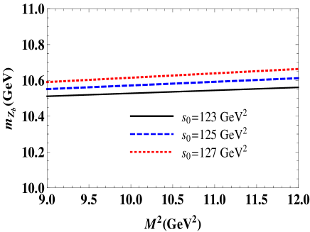
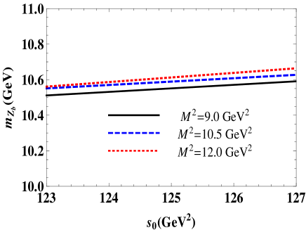
Figure 1: The mass of the $Z_{b}$ state vs Borel parameter $M^{2}$ at fixed $s_{0}$ (left panel), and continuum threshold $s_{0}$ at fixed $M^{2}$ (right panel).

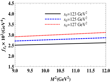
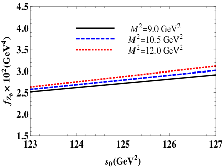
Figure 2: The dependence of the current coupling $f_{Z_{b}}$ of the $Z_{b}$ resonance on the Borel parameter at chosen values of $s_{0}$ (left panel), and on the $s_{0}$ at fixed $M^{2}$ (right panel).

III Decay channels $Z_{b}\to\Upsilon(nS)\pi,\ n=1,\ 2,\ 3.$

This section is devoted to the calculation of the width of $Z_{b}\rightarrow\Upsilon(nS)\pi,\,\ n=1,\,2,\,3$ decays. To this end we determine the strong couplings $g_{Z_{b}\Upsilon_{n}\pi},\ n=1,2,3$ (in formulas we utilize $\Upsilon_{n}\equiv\Upsilon(nS)$ ) using QCD sum rules on the light-cone in conjunction with ideas of a soft-meson approximation.

We start from analysis of the vertices $Z_{b}\Upsilon_{n}\pi$ aiming to calculate $g_{Z_{b}\Upsilon_{n}\pi}$, and therefore consider the correlation function

$$\Pi_{\mu\nu}(p,q)=i\int d^{4}xe^{ipx}\langle\pi(q)|\mathcal{T}\{J_{\mu}^{\Upsilon}(x)J_{\nu}^{Z_{b}\dagger}(0)\}|0\rangle,$$ (17)

where

$$J_{\mu}^{\Upsilon}(x)=\overline{b}_{i}(x)\gamma_{\mu}b_{i}(x),$$ (18)

is the interpolating current for mesons $\Upsilon(nS)$. Here $p$, $q$ and $p^{\prime}=p+q$ are the momenta of $\Upsilon(nS)$, $\pi$ and $Z_{b}$, respectively.

To derive sum rules for the couplings $g_{Z_{b}\Upsilon_{n}\pi}$, we calculate $\Pi_{\mu\nu}(p,q)$ in terms of the physical degrees of freedom. It is not difficult to obtain

$$\Pi_{\mu\nu}^{\mathrm{Phys}}(p,q)=\sum_{n=1}^{3}\frac{\langle 0|J_{\mu}^{\Upsilon}|\Upsilon_{n}\left(p\right)\rangle}{p^{2}-m_{\Upsilon(nS)}^{2}}\langle\Upsilon_{n}\left(p\right)\pi(q)|Z_{b}(p^{\prime})\rangle$$

$$\times\frac{\langle Z_{b}(p^{\prime})|J_{\nu}^{Z_{b}\dagger}|0\rangle}{p^{\prime 2}-m_{Z_{b}}^{2}}+\ldots,$$ (19)

where the dots denote contribution of the higher resonances and continuum states.

We introduce the matrix elements

$$\langle 0|J_{\mu}^{\Upsilon}|\Upsilon_{n}\left(p\right)\rangle=f_{\Upsilon_{n}}m_{\Upsilon_{n}}\varepsilon_{\mu},$$

$$\langle Z_{b}(p^{\prime})|J_{\nu}^{Z_{b}\dagger}|0\rangle=f_{Z_{b}}m_{Z_{b}}\varepsilon_{\nu}^{\prime\ast},$$

$$\langle\Upsilon_{n}\left(p\right)\pi(q)|Z_{b}(p^{\prime})\rangle=g_{Z_{b}\Upsilon_{n}\pi}\left[(p\cdot p^{\prime})\right.$$

$$\left.\times(\varepsilon^{\ast}\cdot\varepsilon^{\prime})-(p\cdot\varepsilon^{\prime})(p^{\prime}\cdot\varepsilon^{\ast})\right],$$ (20)

where $f_{\Upsilon_{n}},\,m_{\Upsilon_{n}},\,\varepsilon_{\mu}$ are the decay constant, mass and polarization vector of the $\Upsilon(nS)$ meson, and $\varepsilon_{\nu}^{\prime}$ is the polarization vector of the $Z_{b}$ state.

Having used Eq. (20) we rewrite the correlation function in the form

$$\Pi_{\mu\nu}^{\mathrm{Phys}}(p,q)=\sum_{n=1}^{3}\frac{g_{Z_{b}\Upsilon_{n}\pi}f_{\Upsilon_{n}}f_{Z_{b}}m_{Z_{b}}m_{\Upsilon_{n}}}{\left(p^{\prime 2}-m_{Z_{b}}^{2}\right)\left(p^{2}-m_{\Upsilon_{n}}^{2}\right)}$$

$$\times\left(\frac{m_{Z_{b}}^{2}+m_{\Upsilon_{n}}^{2}}{2}g_{\mu\nu}-p_{\mu}^{\prime}p_{\nu}\right)+\ldots.$$ (21)

For calculation of the strong couplings we choose to work with the structure $\sim g_{\mu\nu}$. To this end, we have to isolate the invariant function $\Pi^{\mathrm{Phys}}(p^{2},p^{\prime 2})$ corresponding to this structure and find its double Borel transformation. But, it is known that in the case of vertices involving a tetraquark and two conventional mesons one has to set $q=0$ Agaev:2016dev . This is connected with the fact that interpolating current for the tetraquark is composed of four quarks fields and after contracting two of them in the correlation function $\Pi_{\mu\nu}(p,q)$ with relevant quark fields from the heavy meson’s current we encounter a situation when remaining quarks are located at the same space-time point. These quarks fields, sandwiched between a light meson and vacuum instead of generating light meson’s distribution amplitudes create its local matrix elements. Then, in accordance with the four-momentum conservation at such vertices we have to set $q=0$. In QCD light-cone sum rules the limit $q\rightarrow 0$ when a light-cone expansion reduces to a short-distant expansion over local matrix elements is known as a ”soft-meson approximation”. The mathematical methods to handle soft-meson limit were elaborated in Refs. Belyaev:1994zk ; Ioffe:1983ju , and were successfully applied to tetraquark vertices in our works Agaev:2016ijz ; Agaev:2016dsg ; Agaev:2017foq ; Agaev:2017tzv . In soft limit $p^{\prime}=p$ and relevant invariant amplitudes in the correlation function depend only on one variable $p^{2}$. In the present work we use this approach which implies calculation of the correlation function with the equal initial and final momenta $p^{\prime}=p$, and dealing with the obtained double pole terms.

In fact, in the limit $p=p^{\prime}$ we replace in Eq. (21)

$$\frac{1}{\left(p^{\prime 2}-m_{Z_{b}}^{2}\right)\left(p^{2}-m_{\Upsilon_{n}}^{2}\right)}$$

by double pole factors

$$\frac{1}{\left(p^{2}-m_{n}^{2}\right)^{2}},$$

where $m_{n}^{2}=(m_{Z_{b}}^{2}+m_{\Upsilon_{n}}^{2})/2$, and carry out the Borel transformation over $p^{2}$. Then for the Borel transformation of $\Pi^{\mathrm{Phys}}(p^{2})$ we get

$$\mathcal{B}\Pi^{\mathrm{Phys}}(p^{2})=\sum_{n=1}^{3}g_{Z_{b}\Upsilon_{n}\pi}f_{\Upsilon_{n}}f_{Z_{b}}m_{Z_{b}}m_{\Upsilon_{n}}$$

$$\times m_{n}^{2}\frac{e^{-m_{n}^{2}/M^{2}}}{M^{2}}+\ldots.$$ (22)

Now one has to derive the correlation function in terms of the quark-gluon degrees of freedom and find the QCD side of the sum rules. Contracting of heavy quark fields in Eq. (17) yields

$$\Pi_{\mu\nu}^{\mathrm{QCD}}(p,q)=\int d^{4}xe^{ipx}\frac{\epsilon\widetilde{\epsilon}}{\sqrt{2}}\left[\gamma_{5}\widetilde{S}_{b}^{ib}(x){}\gamma_{\mu}\right.$$

$$\left.\times\widetilde{S}_{b}^{ei}(-x){}\gamma_{\nu}+\gamma_{\nu}\widetilde{S}_{b}^{ib}(x){}\gamma_{\mu}\widetilde{S}_{b}^{ei}(-x){}\gamma_{5}\right]_{\alpha\beta}$$

$$\times\langle\pi(q)|\overline{u}_{\alpha}^{a}(0)d_{\beta}^{d}(0)|0\rangle,$$ (23)

where $\alpha$ and $\beta$ are the spinor indices. We continue and use the expansion

$$\overline{u}_{\alpha}^{a}d_{\beta}^{d}\rightarrow\frac{1}{4}\Gamma_{\beta\alpha}^{j}\left(\overline{u}^{a}\Gamma^{j}d^{d}\right),$$ (24)

where $\Gamma^{j}$ is the full set of Dirac matrixes

$$\Gamma^{j}=\mathbf{1,\ }\gamma_{5},\ \gamma_{\lambda},\ i\gamma_{5}\gamma_{\lambda},\ \sigma_{\lambda\rho}/\sqrt{2}.$$

Replacing $\overline{u}_{\alpha}^{a}d_{\beta}^{d}$ in Eq. (23) by this expansion and performing summations over color indices it is not difficult to determine local matrix elements of pion which contribute to $\Pi_{\mu\nu}^{\mathrm{QCD}}(p,q)$ (see, Ref. Agaev:2016dev for details). It turns out that in soft limit the pion’s local matrix element which contributes to $\mathrm{Im}\Pi_{\mu\nu}^{\mathrm{QCD}}(p,q=0)$ is

$$\langle 0|\overline{d}(0)i\gamma_{5}u(0)|\pi(q)\rangle=f_{\pi}\mu_{\pi},$$ (25)

where

$$\mu_{\pi}=\frac{m_{\pi}^{2}}{m_{u}+m_{d}}.$$

After fixing in $\mathrm{Im}\Pi_{\mu\nu}^{\mathrm{QCD}}(p,q=0)$ the structure $\sim g_{\mu\nu}$ it is straightforward to extract $\rho_{\Upsilon}^{\mathrm{QCD}}(s)$ as a sum of the perturbative and nonperturbative components:

$$\rho_{\Upsilon}^{\mathrm{QCD}}(s)=\frac{f_{\pi}\mu_{\pi}}{12\sqrt{2}}\left[\rho^{\mathrm{pert.}}(s)+\rho^{\mathrm{n.-pert.}}(s)\right]$$ (26)

The $\rho_{\Upsilon}^{\mathrm{QCD}}(s)$ can be obtained after replacement $m_{c}\rightarrow m_{b}$ from the spectral density of $\ Z_{c}\rightarrow J/\psi\pi$ decay calculated in Refs. Agaev:2016dev ; Agaev:2017tzv . Its perturbative component $\rho^{\mathrm{pert.}}(s)$ has a simple form and reads

$$\rho^{\mathrm{pert.}}(s)=\frac{(s+2m_{b}^{2})\sqrt{s(s-4m_{b}^{2})}}{\pi^{2}s}.$$ (27)

The nonperturbative contribution $\rho^{\mathrm{n.-pert.}}(s)$ depends on the vacuum expectation values of the gluon operators and contains terms of four, six and eight dimensions. Its explicit expression was presented in Appendix of Ref. Agaev:2017tzv .

The continuum subtraction in the case under consideration can be done using the quark-hadron duality, which lead the desired sum rule for strong couplings. We get:

$$\sum_{n=1}^{3}g_{Z_{b}\Upsilon_{n}\pi}f_{\Upsilon_{n}}f_{Z_{b}}m_{Z_{b}}m_{\Upsilon_{n}}m_{n}^{2}\frac{e^{-m_{n}^{2}/M^{2}}}{M^{2}}$$ (28)

$$= \int_{4m_{b}^{2}}^{s_{0}}dse^{-s/M^{2}}\rho_{\Upsilon}^{\mathrm{QCD}}(s).$$

Here some comments are in order on obtained expression (28). It is known, that the soft limit considerably simplifies the QCD side of light-cone sum rule expressions Belyaev:1994zk . At the same time, in the limit $q\rightarrow 0$ the phenomenological side of the sum rules gains contributions which are not suppressed relative to a main term. In our case the main term corresponds to vertex $Z_{b}\Upsilon(1S)\pi$, where the tetraquark and mesons are ground-state particles. Additional contributions emerge due to vertices $Z_{b}\Upsilon\pi$ where some of particles (or all of them) are on their excited states. In Eq. (28) terms corresponding to vertices $Z_{b}\Upsilon(2S)\pi$ and $Z_{b}\Upsilon(3S)\pi$ belong to this class of contributions. When we are interested in extraction of parameters of a vertex built of only ground-state particles these additional contributions are undesired contaminations which may affect accuracy of calculations. A technique to eliminate them from sum rules is also well known Belyaev:1994zk ; Ioffe:1983ju . To this end, in accordance with elaborated recipies one has to act by the operator

$$\mathcal{P}(M^{2},m_{n}^{2})=\left(1-M^{2}\frac{d}{dM^{2}}\right)M^{2}e^{m_{n}^{2}/M^{2}},$$ (29)

to Eq. (28). In the present work we are going to evaluate three strong couplings $g_{Z_{b}\Upsilon_{n}\pi}$ and, therefore use the original form of the sum rule given by Eq. (28). But it provides only one equality for three unknown quantities. In order to get two additional equations we act by operators $d/d(-1/M^{2})$ and $d^{2}/d(-1/M^{2})^{2}$ to both sides of Eq. (28) and solve obtained equations to find $g_{Z_{b}\Upsilon_{n}\pi}$.

The width of the decays $Z_{b}\rightarrow\Upsilon(nS)\pi,\ n=1,2,3$ can be calculated applying the standard methods and has the same form as in the case of the decay $Z_{c}\rightarrow J/\psi\pi$. After evident replacements in corresponding formula we get:

$$\Gamma\left(Z_{b}\rightarrow\Upsilon_{n}\pi\right)=\frac{g_{Z_{b}\Upsilon_{n}\pi}^{2}m_{\Upsilon_{n}}^{2}}{24\pi}\lambda\left(m_{Z_{b}},\ m_{\Upsilon_{n}},m_{\pi}\right)$$

$$\times\left[3+\frac{2\lambda^{2}\left(m_{Z_{b}},\ m_{\Upsilon_{n}},m_{\pi}\right)}{m_{\Upsilon_{n}}^{2}}\right],$$ (30)

where

$$\lambda(a,\ b,\ c)=\frac{\sqrt{a^{4}+b^{4}+c^{4}-2\left(a^{2}b^{2}+a^{2}c^{2}+b^{2}c^{2}\right)}}{2a}.$$

The key component in Eq. (30) is the strong coupling $g_{Z_{b}\Upsilon_{n}\pi}$. Relevant sum rules contain spectroscopic parameters of the tetraquark $Z_{b}$, and mesons $\Upsilon(nS)$ and $\pi$. The mass and current coupling of the $Z_{b}$ resonance have been calculated in the previous section. For numerical computations we take masses $m_{\Upsilon_{n}}$ and decay constants $f_{\Upsilon_{n}}$ of the mesons $\Upsilon(nS)$ from Ref. Olive:2016xmw . The relevant information is shown in Table 1.

Parameters	Values (in ($\mathrm{MeV}$)
$m_{\Upsilon_{1}}$	$9460.30\pm 0.26$
$f_{\Upsilon_{1}}$	$708\pm 8$
$m_{\Upsilon_{2}}$	$10023.26\pm 0.31$
$f_{\Upsilon_{2}}$	$482\pm 10$
$m_{\Upsilon_{3}}$	$10355.2\pm 0.5$
$f_{\Upsilon_{3}}$	$346\pm 50$
$m_{\pi}$	$139.57061\pm 0.00024$
$f_{\pi}$	$131.5$

Table 1: Spectroscopic parameters of the mesons $\Upsilon_{nS}$ and $\pi$.

In calculations the Borel parameter $M^{2}$ and continuum threshold $s_{0}$ are varied within regions

$$M^{2}=10-13\ \mathrm{GeV}^{2},\ s_{0}=124-128\ \mathrm{GeV}^{2},$$ (31)

which are almost identical to similar working windows in the mass and current coupling calculations being slightly shifted towards larger values.

For the couplings $g_{Z_{b}\Upsilon_{n}\pi}$ we obtain (in $\mathrm{GeV}^{-1}$):

$$g_{Z_{b}\Upsilon_{1}\pi}=0.019\pm 0.005,\ \,g_{Z_{b}\Upsilon_{2}\pi}=0.090\pm 0.031,$$

$$g_{Z_{b}\Upsilon_{3}\pi}=0.104\pm 0.031.$$ (32)

For the width of the decays $Z_{b}\rightarrow\Upsilon(nS)\pi$ these couplings lead to predictions

$$\Gamma(Z_{b}\rightarrow\Upsilon(1S)\pi)=1.36\pm 0.43\ \mathrm{MeV},$$

$$\Gamma(Z_{b}\rightarrow\Upsilon(2S)\pi)=17.18\pm 5.01\ \mathrm{MeV},$$

$$\Gamma(Z_{b}\rightarrow\Upsilon(3S)\pi)=8.27\pm 2.69\ \mathrm{MeV}.$$ (33)

Obtained predictions for width of the decays $\Gamma(Z_{b}\rightarrow\Upsilon(nS)\pi)$ are final results of this section and will be used for comparison with the experimental data.

IV $Z_{b}\to h_{b}(1P)\pi$ and $Z_{b}\to h_{b}(2P)\pi$ decays

The second class of decays which we consider contains two processes $Z_{b}\rightarrow h_{b}(mP)\pi,\ m=1,2$. We follow the same prescriptions as in the case of $Z_{b}\rightarrow\Upsilon(nP)\pi$ decays and derive sum rules for the strong couplings $g_{Z_{b}h_{b}\pi}$ and $g_{Z_{b}h_{b}^{\prime}\pi}$ (hereafter we employ short-hand notations $h_{b}\equiv h_{b}(1P)$ and $h_{b}^{\prime}\equiv h_{b}(2P)$). From analysis performed in the previous section it is clear that corresponding sum rules will depend on numerous input parameters including mass and decay constant of the mesons $h_{b}(1P)$ and $h_{b}(2P)$. Information on the spectroscopic parameters of $h_{b}(1P)$ is available in the literature. Indeed, in the context of QCD sum rule method mass and decay constant of $h(1P)$ were calculated in Ref. Wang:2012gj . But decay constant $f_{h_{b}^{\prime}}$ of the meson $h_{b}(2P)$ was not evaluated, therefore in the present work we have first to find the parameters $m_{h_{b}^{\prime}}$ and $f_{h_{b}^{\prime}}$, and turn after that to our main task.

IV.1 Spectroscopic parameters of the mesons $h_{b}(1P)$ and $h_{b}(2P)$

The meson $h(1P)$ is the spin-singlet $P$-wave bottomonium with quantum numbers $J^{PC}=1^{+-}$, whereas $h(2P)$ is its first radial excitation. Parameters of the $h_{b}(1P)$ and $h_{b}(2P)$ mesons in the framework of QCD two-point sum rule method can be extracted from the correlation function

$$\Pi_{\mu\nu\alpha\beta}(p)=i\int d^{4}xe^{ipx}\langle 0|\mathcal{T}\left\{J_{\mu\nu}^{h}(x)J_{\alpha\beta}^{h\dagger}(0)\right\}|0\rangle,$$ (34)

where the interpolating current for $h_{b}(mP)$ mesons is chosen as

$$J_{\mu\nu}^{h}(x)=\overline{b}^{i}(x)\sigma_{\mu\nu}\gamma_{5}b^{i}(x).$$ (35)

It couples both to $h_{b}(1P)$ and $h_{b}(2P)$, and is convenient for analysis of $J^{PC}=1^{+-}$ mesons (see, Ref. Wang:2012gj ).

In order to find required sum rules we use ”ground-state+first radial excitation+continuum” scheme. Then, the physical side of the sum rule

$$\Pi_{\mu\nu\alpha\beta}^{\mathrm{Phys}}(p)=\frac{\langle 0|J_{\mu\nu}^{h}|h_{b}(p)\rangle\langle h_{b}(p)|J_{\alpha\beta}^{h\dagger}(0)|0\rangle}{m_{h_{b}}^{2}-p^{2}}$$

$$+\frac{\langle 0|J_{\mu\nu}^{h}|h_{b}^{\prime}(p)\rangle\langle h_{b}^{\prime}(p)|J_{\alpha\beta}^{h\dagger}(0)|0\rangle}{m_{h_{b}^{\prime}}^{2}-p^{2}}+\ldots,$$ (36)

contains two terms of interest and also contribution of higher resonances and continuum states denoted by dots. We continue by introducing the matrix elements

$$\langle 0|J_{\mu\nu}^{h}|h_{b}^{(\prime)}(p)\rangle=f_{h_{b}^{(\prime)}}(\varepsilon_{\mu}^{(\prime)}p_{\nu}-\varepsilon_{\nu}^{(\prime)}p_{\mu}),$$ (37)

and recast the correlation function $\Pi_{\mu\nu\alpha\beta}^{\mathrm{Phys}}(p)$ into the form

$$\Pi_{\mu\nu\alpha\beta}^{\mathrm{Phys}}(p)=\frac{f_{h_{b}}^{2}}{m_{h_{b}}^{2}-p^{2}}\left[\widetilde{g}_{\mu\alpha}p_{\nu}p_{\beta}-\widetilde{g}_{\mu\beta}p_{\nu}p_{\alpha}\right.$$

$$\left.-\widetilde{g}_{\nu\alpha}p_{\mu}p_{\beta}+\widetilde{g}_{\nu\beta}p_{\mu}p_{\alpha}\right]+\frac{f_{h_{b}^{\prime}}^{2}}{m_{h_{b}^{\prime}}^{2}-p^{2}}\left[\widetilde{g}_{\mu\alpha}^{\prime}p_{\nu}p_{\beta}\right.$$

$$\left.-\widetilde{g}_{\mu\beta}^{\prime}p_{\nu}p_{\alpha}-\widetilde{g}_{\nu\alpha}^{\prime}p_{\mu}p_{\beta}+\widetilde{g}_{\nu\beta}^{\prime}p_{\mu}p_{\alpha}\right],$$ (38)

where

$$\widetilde{g}_{\mu\alpha}^{(\prime)}=-g_{\mu\alpha}+\frac{p_{\mu}p_{\alpha}}{m_{h_{b}^{(\prime)}}^{2}}.$$

The Borel transformation of $\Pi_{\mu\nu\alpha\beta}^{\mathrm{Phys}}(p)$ can be obtained by simple replacements in Eq. (38)

$$\mathcal{B}\frac{f_{h_{b}^{(\prime)}}^{2}}{m_{h_{b}^{(\prime)}}^{2}-p^{2}}=f_{h_{b}^{(\prime)}}^{2}e^{-m_{h_{b}^{(\prime)}}^{2}/M^{2}}.$$

The obtained by this way expression contains numerous Lorentz structures which, in general, may be employed to derive sum rules for masses and decay constants: We choose a structure $\sim\widetilde{g}_{\mu\alpha}p_{\nu}p_{\beta}$ to extract sum rules. The term with the same structure should be isolated in the Borel transformation of $\Pi_{\mu\nu\alpha\beta}^{\mathrm{QCD}}(p)$, i. e. in expression of the correlation function calculated using quark-gluon degrees of freedom.

After simple computations for $\Pi_{\mu\nu\alpha\beta}^{\mathrm{QCD}}(p)$ we get

$$\Pi_{\mu\nu\alpha\beta}^{\mathrm{QCD}}(p) = i\int d^{4}xe^{ipx}\mathrm{Tr}\left[\gamma_{5}\sigma_{\alpha\beta}S_{b}^{ji}(-x)\right.$$ (39)

$$\left.\times\sigma_{\mu\nu}\gamma_{5}S_{b}^{ij}(x)\right].$$

The following operations are standard manipulations; they imply Borel transforming of $\Pi_{\mu\nu\alpha\beta}^{\mathrm{QCD}}(p)$, equating the structures $\sim\widetilde{g}_{\mu\alpha}p_{\nu}p_{\beta}$ in both the physical and QCD sides of obtained equality, and subtracting the continuum contribution. We obtain the second sum rule by acting on first one by $d/d(-1/M^{2})$. These two sum rules allow us to evaluate masses and decay constants of the $h_{b}(1P)$ and $h_{b}(2P)$ mesons. At the first stage we employ ”ground-state +continuum” scheme, which is commonly used in sum rule computations. This means that we include the excited $h_{b}(2P)$ meson into the ”higher resonances and continuum” part of sum rules and fix working windows for $M^{2}$ and $s_{0}$. From these sum rules we extract spectroscopic parameters of the $h_{b}(1P)$ meson $m_{h_{b}}$ and $f_{h_{b}}$. At the next step we employ the same sum rules with $s_{0}^{\ast}>s_{0}$ to embrace contribution arising from $h_{b}(2P)$, and treat $m_{h_{b}}$ and $f_{h_{b}}$ evaluated at the first stage as fixed parameters.

Numerical analysis restricts variation of the parameters $M^{2}$ and $s_{0}$ within the regions

$$M^{2}=10-12\ \mathrm{GeV}^{2},\ s_{0}=103-105\ \mathrm{GeV}^{2},$$

and we find

$$m_{h_{b}}=9886_{-78}^{+81}\ \mathrm{MeV,\ \ }f_{h_{b}}=325_{-57}^{+61}\ \ \mathrm{MeV}.$$ (40)

At the next step we use

$$\ s_{0}^{\ast}=109-111\ \mathrm{GeV}^{2},$$

and get

$$m_{h_{b}^{\prime}}=10331_{-117}^{+108}\ \mathrm{MeV,\ \ }f_{h_{b}^{\prime}}=286_{-53}^{+58}\ \ \mathrm{MeV}.$$ (41)

Parameters of the $h_{b}(2P)$ meson are among essentially new results of the present work, therefore in Figs. 3 and 4 we demonstrate $m_{h_{b}(2P)}$ and $f_{h_{b}(2P)}$ as functions of the Borel parameter $M^{2}$ and continuum threshold $s_{0}$.

Comparing our results with experimental information on masses of the $h_{b}(mP)$ mesons Olive:2016xmw

$$m_{h_{b}} = 9899.3\pm 0.8\ \mathrm{MeV},\$$

$$m_{h_{b}^{\prime}} = 10259.8\pm 1.2\ \mathrm{MeV},$$

we see a reasonable agreement between them.

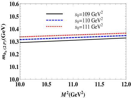
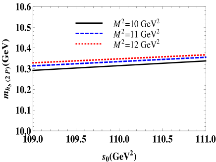
Figure 3: The mass of the meson $h_{b}(2P)$ as a function of the Borel parameter $M^{2}$ at fixed $s_{0}$ (left panel), and as a function of the continuum threshold $s_{0}$ at fixed $M^{2}$ (right panel).

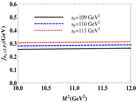
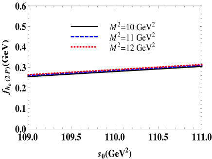
Figure 4: The dependence of the decay constant $f_{h_{b}(2P)}$ on the Borel parameter at chosen values of $s_{0}$ (left panel), and on the $s_{0}$ at fixed $M^{2}$ (right panel).

IV.2 Width of decays $Z_{b}\rightarrow h_{b}(1P)\pi$ and $Z_{b}\rightarrow h_{b}(2P)\pi$

Analysis of the vertices $Z_{b}h_{b}(mP)\pi$ does not differ from analogous investigation carried out in the previous section. We start here from the correlator

$$\Pi_{\mu\nu\lambda}(p,q)=i\int d^{4}xe^{ipx}\langle\pi(q)|\mathcal{T}\{J_{\mu\nu}^{h}(x)J_{\lambda}^{Z_{b}\dagger}(0)\}|0\rangle,$$

and for its phenomenological representation get

$$\Pi_{\mu\nu\lambda}^{\mathrm{Phys}}(p,q)=\frac{\langle 0|J_{\mu\nu}^{h}|h_{b}\left(p\right)\rangle}{p^{2}-m_{h_{b}}^{2}}\langle h_{b}\left(p\right)\pi(q)|Z_{b}(p^{\prime})\rangle$$

$$\times\frac{\langle Z_{b}(p^{\prime})|J_{\lambda}^{Z_{b}\dagger}|0\rangle}{p^{\prime 2}-m_{Z_{b}}^{2}}+\frac{\langle 0|J_{\mu\nu}^{h}|h_{b}^{\prime}\left(p\right)\rangle}{p^{2}-m_{h_{b}^{\prime}}^{2}}$$ (42)

$$\times\langle h_{b}^{\prime}\left(p\right)\pi(q)|Z_{b}(p^{\prime})\rangle\frac{\langle Z_{b}(p^{\prime})|J_{\lambda}^{Z_{b}\dagger}|0\rangle}{p^{\prime 2}-m_{Z_{b}}^{2}}\ldots.$$ (43)

The $\Pi_{\mu\nu\lambda}^{\mathrm{Phys}}(p,q)$ contains two terms of initerest and contributions coming from higher resonances and continuum shown above as dots. Using matrix elements of the currents $J_{\mu\nu}^{h}$ and $J_{\lambda}^{Z_{b}}$ and introducing the vertex

$$\langle h_{b}^{(\prime)}\left(p\right)\pi(q)|Z_{b}(p^{\prime})\rangle=g_{Z_{b}h_{b}^{(\prime)}\pi}\epsilon_{\alpha\beta\gamma\delta}\varepsilon_{\alpha}^{\ast}(p)\varepsilon_{\beta}^{\prime}(p^{\prime})p_{\gamma}p_{\delta}^{\prime},$$ (44)

we find

$$\Pi_{\mu\nu\lambda}^{\mathrm{Phys}}(p,q)=\frac{f_{Z_{b}}m_{Z_{b}}}{\left(p^{\prime 2}-m_{Z_{b}}^{2}\right)}\left[\frac{g_{Z_{b}h_{b}\pi}f_{h_{b}}}{\left(p^{2}-m_{h_{b}}^{2}\right)}+\frac{g_{Z_{b}h_{b}^{\prime}\pi}f_{h_{b}^{\prime}}}{\left(p^{2}-m_{h_{b}^{\prime}}^{2}\right)}\right]$$

$$\times\left(\epsilon_{\mu\lambda\gamma\delta}p_{\gamma}p_{\delta}^{\prime}p_{\nu}-\epsilon_{{}_{\nu}\lambda\gamma\delta}p_{\gamma}p_{\delta}^{\prime}p_{\mu}\right)+\ldots$$ (45)

The same correlation function expressed in terms of quark propagators takes the following form

$$\Pi_{\mu\nu\lambda}^{\mathrm{QCD}}(p,q)=\int d^{4}xe^{ipx}\frac{\epsilon\widetilde{\epsilon}}{\sqrt{2}}\left[\gamma_{5}\widetilde{S}_{b}^{ib}(x){}\gamma_{5}\sigma_{\mu\nu}\right.$$

$$\left.\times\widetilde{S}_{b}^{ei}(-x){}\gamma_{\lambda}+\gamma_{\lambda}\widetilde{S}_{b}^{ib}(x){}\gamma_{5}\sigma_{\mu\nu}\widetilde{S}_{b}^{ei}(-x){}\gamma_{5}\right]_{\alpha\beta}$$

$$\times\langle\pi(q)|\overline{u}_{\alpha}^{a}(0)d_{\beta}^{d}(0)|0\rangle.$$ (46)

Expanding $\overline{u}_{\alpha}^{a}d_{\beta}^{d}$ in accordance with Eq. (24) and substituting into Eq. (46) local matrix elements of the pion we obtain $\Pi_{\mu\nu\lambda}^{\mathrm{QCD}}(p,q)$ which can be matched to $\Pi_{\mu\nu\lambda}^{\mathrm{Phys}}(p,q)$ to fix same tensor structures. In order to derive sum rule we use structures $\sim\epsilon_{\mu\lambda\gamma\delta}p_{\gamma}p_{\delta}^{\prime}p_{\nu}$ from both sides of equality. The pion matrix element that contributes to this structure is

$$0|\overline{d}(0)\gamma_{5}\gamma_{\mu}u(0)|\pi(q)\rangle=if_{\pi}q_{\mu}.$$

In fact, it can be included into the chosen structure after replacement $q_{\mu}=p_{\mu}^{\prime}-p_{\mu}$ .

In obtained equality we apply the soft limit $q\rightarrow 0$ ($p=p^{\prime}$) and perform the Borel transformation on variable $p^{2}$. This operations leads to a sum rule for two strong couplings $g_{Z_{b}h_{b}\pi}$ and $g_{Z_{b}h_{b}^{\prime}\pi}$. The second expression is obtained from the first one by applying the operator $d/d(-1/M^{2})$ .

The principal output of these calculations, i.e. the spectral density $\rho_{\mathrm{h}}^{\mathrm{QCD}}(s)$ reads

$$\rho_{\mathrm{h}}^{\mathrm{QCD}}(s)=\frac{f_{\pi}}{12\sqrt{2}}\left[\rho^{\mathrm{pert.}}(s)+\rho^{\mathrm{n.-pert.}}(s)\right],$$ (47)

where its perturbative part is given by the formula

$$\rho^{\mathrm{pert.}}(s)=\frac{(s+2m_{b}^{2})\sqrt{s(s-4m_{b}^{2})}}{\pi^{2}s^{2}}.$$ (48)

The nonperturbative component of $\rho_{\mathrm{h}}^{\mathrm{QCD}}(s)$ includes contributions up to eight dimensions and has the form

$$\rho^{\mathrm{n.-pert.}}(s)=\Big{\langle}\frac{\alpha_{s}G^{2}}{\pi}\Big{\rangle}m_{b}^{2}\int_{0}^{1}f_{1}(z,s)dz$$

$$+\Big{\langle}g_{s}^{3}G^{3}\Big{\rangle}\int_{0}^{1}f_{2}(z,s)dz$$

$$-\Big{\langle}\frac{\alpha_{s}G^{2}}{\pi}\Big{\rangle}^{2}m_{b}^{4}\int_{0}^{1}f_{3}(z,s)dz.$$ (49)

Here the functions $f_{k}(z,s)$ are:

$$f_{1}(z,s)=\frac{1}{3}\frac{(1+3r)}{r^{2}}\delta^{(2)}(s-\Phi),$$

$$f_{2}(z,s)=\frac{1}{15\cdot 2^{6}}\frac{1}{r^{4}}\left\{4r^{2}(3+17r+21r^{2})\delta^{(2)}(s-\Phi)\right.$$

$$+2r\left[sr^{2}(4+13r)+3m_{b}^{2}(3+16r+18r^{2})\right]\delta^{(3)}(s-\Phi)$$

$$+\left[s^{2}r^{4}+6m_{b}^{2}sr^{2}(1+3r)-7m_{b}^{4}(1+5r+5r^{2})\right]$$

$$\left.\times\delta^{(4)}(s-\Phi)\right\},$$

$$f_{3}(z,s)=\frac{1}{54}\frac{\pi^{2}}{r^{2}}\delta^{(5)}(s-\Phi),$$

where

$$\ r=z(z-1),\ \Phi=\frac{m_{b}^{2}}{z(1-z)}.$$

In the expressions above the Dirac delta function $\ \delta^{(n)}(s-\Phi)$ is defined in accordance with

$$\delta^{(n)}(s-\Phi)=\frac{d^{n}}{ds^{n}}\delta(s-\Phi).$$ (50)

The width of the decays $Z_{b}\rightarrow h_{b}(1P)\pi$ and $Z_{b}\rightarrow h_{b}(2P)\pi$ are calculated using the formula

$$\Gamma(Z_{b}\rightarrow h_{b}(mP)\pi)=g_{Z_{b}h_{b}(mP)\pi}^{2}\frac{\lambda\left(m_{Z_{b}},\ m_{h(mP)},m_{\pi}\right)^{3}}{12\pi}.$$

In numerical computations we employ parameters of the $h_{b}(mP)$ mesons obtained in the previous subsection. The working regions of the Borel parameter $M^{2}$ and continuum threshold $s_{0}$ are the same as in analysis of $Z_{b}\rightarrow\Upsilon(nS)\pi$ decays. Below we provide our results for the strong couplings (in units $\mathrm{GeV}^{-1}$)

$$g_{Z_{b}h_{b}\pi}=0.94\pm 0.27,\ \,g_{Z_{b}h_{b}^{\prime}\pi}=3.43\pm 0.93.$$ (51)

In Fig. 5 we plot the coupling $g_{Z_{b}h_{b}^{\prime}\pi}$ as a function of the Borel parameter and continuum threshold to show its dependence on these auxiliary parameters. It is easy to see that theoretical errors are within limits accepted in sum rule calculations.

Using Eq. (51) it is not difficult we evaluate width of the decays:

$$\Gamma(Z_{b} \rightarrow h_{b}(1P)\pi)=6.30\pm 1.76\ \mathrm{MeV,}$$

$$\Gamma(Z_{b} \rightarrow h_{b}(2P)\pi)=7.35\pm 2.13\ \mathrm{MeV.}$$ (52)

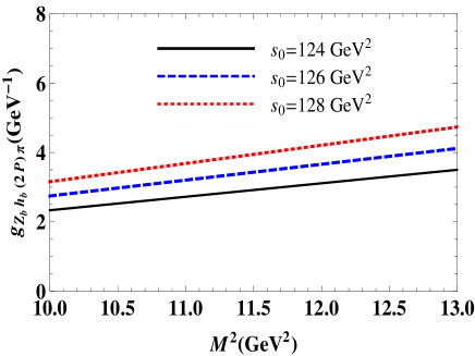
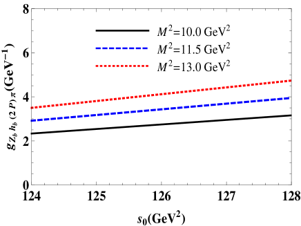
Figure 5: The coupling $g_{Z_{b}h_{b}^{\prime}\pi}$ vs Borel parameter $M^{2}$ (left panel), and continuum threshold $s_{0}$ (right panel).

V Analysis and concluding notes

The experimental data on decay channels of the $Z_{b}(10610)$ resonance were studied and presented in a rather detailed form in Refs. Belle:2011aa ; Garmash:2014dhx ; Garmash:2015rfd . Its full width was estimated as $\Gamma=18.4\pm 2.4\ \mathrm{MeV}$ essential part of which, i.e. approximately $86\%$ of $\Gamma$ is due to decay $Z_{b}\rightarrow B^{+}\overline{B}^{\ast 0}+B^{\ast+}\overline{B}^{0}$. The remaining part of the full width is formed by five decay channels investigated in the present work. It is clear that our results for width of decays $Z_{b}\rightarrow\Upsilon(nS)\pi$ and $Z_{b}\rightarrow h_{b}(nP)\pi$ overshoot the experimental data. Therefore, in the light of present studies we refain from interpretation of the $Z_{b}(10610)$ resonance as a pure diquark-antidiquark $[bu][\overline{b}\overline{d}]$ state.

Nevertheless, encouraging are theoretical predictions for the ratios

$$\mathcal{R(}n)\mathcal{=}\frac{\Gamma(Z_{b}\rightarrow\Upsilon(nS)\pi)}{\Gamma(Z_{b}\rightarrow\Upsilon(1S)\pi)},\mathcal{R(}m)\mathcal{=}\frac{\Gamma(Z_{b}\rightarrow h_{b}(mS)\pi)}{\Gamma(Z_{b}\rightarrow\Upsilon(1S)\pi)},$$ (53)

where we normalize widths of different decay channels to $\Gamma(Z_{b}\rightarrow\Upsilon(1S)\pi)$. The ratio $\mathcal{R}$ can be extracted from available experimental data and calculated from decay widths obtained in the present work. In order to fix existing similarities and differences between theoretical and experimental information on $\mathcal{R}$ we provide two sets of corresponding values in Table 2. It is worth to note that we use latest available experimental information from Ref. Olive:2016xmw .

It is seen that theoretical predictions follow pattern of experimental data: we observe the same hierarchy of theoretical and experimental decay widths. At the time, numerical differences between them are noticeable. Nevertheless, in a result of large errors in both sets, there are sizeable overlap regions for each pair of $\mathcal{R}$s, which demonstrate not only qualitative agreement between them but also quantitative compatibility of two sets.

These observations may help one to understand the nature of the $Z_{b}$ resonance. The Belle Collaboration discovered two $Z_{b}$ and $Z_{b}^{\prime}$ resonances with very close masses. We have calculated parameters of an axial-vector diquark-antidiquark state $[bu][\overline{b}\overline{d}]$, and interpreted it as $Z_{b}$. It is possible to model the second $Z_{b}^{\prime}$ resonance using alternative interpolating current, as it has been emphasized in Sec. II and explore its properties. The current with the same quantum numbers but different color organization may also play a role of such alternative (see, for example, Ref. Agaev:2017foq ). One of possible scenarios implies that observed resonances are admixtures of these tetraquarks, which may fit measured decay widths.

The diquark-antidiquark interpolating current used in the present work can be rewritten as a sum of molecular-type terms. In other words, some of molecular-type currents effectively contribute to our predictions, and by enhancing these components (i.e. by adding them to interpolating current with some coefficients) better agreement with experimental data may be achieved. In other words, the resonances $Z_{b}$ and $Z_{b}^{\prime}$ may ”contain” both the diquark-antidiquark and molecular components.

Finally, $Z_{b}$ and $Z_{b}^{\prime}$ states may have pure molecular structures. But pure molecular-type bound states of mesons are usually broader than diquark-antidiquarks with the same quantum numbers and quark contents. In any case, all these suggestions require additional and detailed investigations.

In the present study we have fulfilled only a part of this program. In the framework of QCD sum rule methods we have calculated the spectroscopic parameters of $Z_{b}$ state by modeling it as diquark-antidiquark state, and found widths five of its observed decay channels. We have also evaluated mass and decay constant of $h_{b}(2P)$ meson, which are necessary for analysis of $Z_{b}\rightarrow h_{b}(2P)\pi$ decay. Calculation of the $Z_{b}$ resonance’s dominant decay channel may be performed, for example, using QCD three-point sum rule approach, which is beyond the scope of the present work. Decays considered here involve excited mesons $\Upsilon(nS)$ and $h(mP)$, parameters of which require detailed analysis in a future. More precise measurements of $Z_{b}$ and $Z_{b}^{\prime}$ partial decays’ width can also help in making a choice between outlined scenarios.

$\mathcal{R}$	$n=2$	$n=3$	$m=1$	$m=2$
Exp. Olive:2016xmw	$6.67_{-2.37}^{+3.11}$	$3.89_{-1.55}^{+2.02}$	$6.48_{-2.45}^{+3.18}$	$8.70_{-3.41}^{+4.39}$
This work	$12.63\pm 5.43$	$6.08\pm 2.76$	$4.63\pm 1.95$	$5.40\pm 2.32$

Table 2: Experimental values and theoretical predictions for $\mathcal{R}$.

References

- (1) S. K. Choi et al. [Belle Collaboration], Phys. Rev. Lett. 100, 142001 (2008).
- (2) R. Aaij et al. [LHCb Collaboration], Phys. Rev. Lett. 112, 222002 (2014).
- (3) R. Aaij et al. [LHCb Collaboration], Phys. Rev. D 92, 112009 (2015).
- (4) R. Mizuk et al. [Belle Collaboration], Phys. Rev. D 78, 072004 (2008).
- (5) M. Ablikim et al. [BESIII Collaboration], Phys. Rev. Lett. 110, 252001 (2013).
- (6) M. Ablikim et al. [BESIII Collaboration], Phys. Rev. Lett. 111, 242001 (2013).
- (7) M. Ablikim et al. [BESIII Collaboration], Phys. Rev. Lett. 112, 132001 (2014).
- (8) K. Chilikin et al. [Belle Collaboration], Phys. Rev. D 90, 112009 (2014).
- (9) A. Bondar et al. [Belle Collaboration], Phys. Rev. Lett. 108, 122001 (2012).
- (10) A. Garmash et al. [Belle Collaboration], Phys. Rev. D 91, 072003 (2015).
- (11) A. Garmash et al. [Belle Collaboration], Phys. Rev. Lett. 116, 212001 (2016)
- (12) S. L. Olsen, T. Skwarnicki and D. Zieminska, arXiv:1708.04012 [hep-ph].
- (13) M. Karliner and H. J. Lipkin, arXiv:0802.0649 [hep-ph].
- (14) X. Liu, Z. G. Luo, Y. R. Liu and S. L. Zhu, Eur. Phys. J. C 61, 411 (2009).
- (15) A. E. Bondar, A. Garmash, A. I. Milstein, R. Mizuk and M. B. Voloshin, Phys. Rev. D 84, 054010 (2011).
- (16) M. B. Voloshin, Phys. Rev. D 84, 031502 (2011).
- (17) A. Ali, C. Hambrock and W. Wang, Phys. Rev. D 85, 054011 (2012).
- (18) A. Ali, L. Maiani, A. D. Polosa and V. Riquer, Phys. Rev. D 91, 017502 (2015).
- (19) L. Maiani, F. Piccinini, A. D. Polosa and V. Riquer, Phys. Rev. D 89, 114010 (2014).
- (20) J. R. Zhang, M. Zhong and M. Q. Huang, Phys. Lett. B 704, 312 (2011).
- (21) Y. Yang, J. Ping, C. Deng and H. S. Zong, J. Phys. G 39, 105001 (2012).
- (22) Z. F. Sun, J. He, X. Liu, Z. G. Luo and S. L. Zhu, Phys. Rev. D 84, 054002 (2011).
- (23) H. W. Ke, X. Q. Li, Y. L. Shi, G. L. Wang and X. H. Yuan, JHEP 1204, 056 (2012).
- (24) C. Y. Cui, Y. L. Liu and M. Q. Huang, Phys. Rev. D 85, 074014 (2012).
- (25) D. V. Bugg, Europhys. Lett. 96, 11002 (2011).
- (26) I. V. Danilkin, V. D. Orlovsky and Y. A. Simonov, Phys. Rev. D 85, 034012 (2012).
- (27) D. Y. Chen, X. Liu and S. L. Zhu, Phys. Rev. D 84, 074016 (2011).
- (28) D. Y. Chen and X. Liu, Phys. Rev. D 84, 094003 (2011).
- (29) M. Cleven, F. K. Guo, C. Hanhart and U. G. Meissner, Eur. Phys. J. A 47, 120 (2011).
- (30) M. Cleven, Q. Wang, F. K. Guo, C. Hanhart, U. G. Meissner and Q. Zhao, Phys. Rev. D 87, 074006 (2013).
- (31) T. Mehen and J. Powell, Phys. Rev. D 88, 034017 (2013).
- (32) Z. G. Wang and T. Huang, Eur. Phys. J. C 74, 2891 (2014).
- (33) Z. G. Wang, Eur. Phys. J. C 74, 2963 (2014).
- (34) Y. Dong, A. Faessler, T. Gutsche and V. E. Lyubovitskij, J. Phys. G 40, 015002 (2013).
- (35) W. Chen, T. G. Steele, H. X. Chen and S. L. Zhu, Phys. Rev. D 92, 054002 (2015).
- (36) X. W. Kang, Z. H. Guo and J. A. Oller, Phys. Rev. D 94, 014012 (2016).
- (37) A. Esposito, A. Pilloni and A. D. Polosa, Phys. Rept. 668, 1 (2017).
- (38) A. Ali, J. S. Lange and S. Stone, Prog. Part. Nucl. Phys. 97, 123 (2017).
- (39) S. S. Agaev, K. Azizi and H. Sundu, Phys. Rev. D 93, 074002 (2016).
- (40) V. M. Belyaev, V. M. Braun, A. Khodjamirian and R. Ruckl, Phys. Rev. D 51, 6177 (1995).
- (41) B. L. Ioffe and A. V. Smilga, Nucl. Phys. B 232, 109 (1984).
- (42) S. S. Agaev, K. Azizi and H. Sundu, Phys. Rev. D 93, 114007 (2016).
- (43) S. S. Agaev, K. Azizi and H. Sundu, Phys. Rev. D 95, 034008 (2017).
- (44) S. S. Agaev, K. Azizi and H. Sundu, Phys. Rev. D95, 114003 (2017).
- (45) S. S. Agaev, K. Azizi and H. Sundu, Phys. Rev. D 96, 034026 (2017).
- (46) C. Patrignani et al. [Particle Data Group], Chin. Phys. C 40, 100001 (2016).
- (47) Z. G. Wang, Eur. Phys. J. C 73, 2533 (2013).