The line shapes of the $Z_{b}(10610)$ and $Z_{b}(10650)$ in the elastic and inelastic channels revisited

Abstract

The most recent experimental data for all measured production and decay channels of the bottomonium-like states $Z_{b}(10610)$ and $Z_{b}(10650)$ are analysed simultaneously using solutions of the Lippmann-Schwinger equations which respect constraints from unitarity and analyticity. The interaction potential in the open-bottom channels $B^{(*)}\bar{B}^{*}+\mbox{c.c.}$ contains short-range interactions as well as one-pion exchange. It is found that the long-range interaction does not affect the line shapes as long as only $S$ waves are considered. Meanwhile, the line shapes can be visibly modified once $D$ waves, mediated by the strong tensor forces from the pion exchange potentials, are included. However, in the fit they get balanced largely by a momentum dependent contact term that appears to be needed also to render the results for the line shapes independent of the cut-off. The resulting line shapes are found to be insensitive to various higher-order interactions included to verify stability of the results. Both $Z_{b}$ states are found to be described by the poles located on the unphysical Riemann sheets in the vicinity of the corresponding thresholds. In particular, the $Z_{b}(10610)$ state is associated with a virtual state residing just below the $B\bar{B}^{*}/\bar{B}{B}^{*}$ threshold while the $Z_{b}(10650)$ state most likely is a shallow state located just above the $B^{*}\bar{B}^{*}$ threshold.

I Introduction

In the last decade, numerous new hadrons have been observed in the charmonium and bottomonium energy region. Of special interest are those that cannot be accommodated by the simple quark-model picture and which are, therefore, referred to as exotic hadrons. For example, the charged states $Z_{b}^{\pm}(10610)$, $Z_{b}^{\pm}(10650)$ Belle:2011aa , $Z_{c}^{\pm}(3900)$ Ablikim:2013mio ; Liu:2013dau , $Z_{c}^{\pm}(4020)$ Ablikim:2013wzq , $Z^{\pm}(4430)$ Choi:2007wga ; Mizuk:2009da ; Chilikin:2013tch ; Aaij:2014jqa which, amongst other channels, decay into quarkonium states and a pion, cannot be conventional $\bar{Q}Q$ (with $Q$ denoting the heavy quark) mesons as their minimal quark contents is four-quark.

The $Z_{b}^{\pm}(10610)$ and $Z_{b}^{\pm}(10650)$ bottomonium-like states were observed by the Belle Collaboration as peaks in the invariant mass distributions of the $\Upsilon(nS)\pi^{\pm}$ ($n=1,2,3$) and $h_{b}(mP)\pi^{\pm}$ ($m=1,2$) subsystems in the dipion transitions from the vector bottomonium $\Upsilon(10860)$ Belle:2011aa . Later, they were confirmed in the elastic $B\bar{B}^{*}$ and $B^{*}\bar{B}^{*}$ channels Adachi:2012cx ; Garmash:2015rfd . At present, both a tetraquark structure Ali:2011ug ; Esposito:2014rxa ; Maiani:2017kyi and a hadronic molecule interpretation Bondar:2011ev ; Cleven:2011gp ; Nieves:2011vw ; Zhang:2011jja ; Yang:2011rp ; Sun:2011uh ; Ohkoda:2011vj ; Li:2012wf ; Ke:2012gm ; Dias:2014pva are claimed to be consistent with the data for these two exotic states. Their proximity to the $B\bar{B}^{*}$ and $B^{*}\bar{B}^{*}$ thresholds together with the fact that those are by far the most dominant decay channels of the $Z_{b}^{\pm}(10610)$ and $Z_{b}^{\pm}(10650)$, respectively, provides a strong support for their molecular interpretation. While some works try to explain the $Z_{b}$’s as a simple kinematical cusps Swanson:2014tra , it was demonstrated in Ref. Guo:2014iya that the narrow structures in the elastic channels necessitate near-threshold poles. The general argument presented there was supported by the explicit analyses presented in Refs. Hanhart:2015cua ; Guo:2016bjq . Also the analysis presented in this work finds poles near the thresholds in conflict with the claims of Ref. Swanson:2014tra .

The literature on the hadronic molecule scenario for the $Z_{b}$ states is already very rich: hadronic and radiative decays are studied in Refs. Voloshin:2011qa ; Ohkoda:2012rj ; Li:2012uc ; Cleven:2013sq ; Dong:2012hc ; Li:2012as ; Ohkoda:2013cea , the contribution of the two $Z_{b}$ states to other processes are considered in Refs. Chen:2011zv ; Chen:2015jgl ; Chen:2016mjn , the heavy-quark spin partners of the $Z_{b}$’s are discussed in Refs. Mehen:2011yh ; Ohkoda:2011vj ; Valderrama:2012jv ; HidalgoDuque:2012pq ; Nieves:2012tt ; Guo:2013sya ; Karliner:2015ina ; Baru:2017gwo , the line shapes and poles position are addressed in Refs. Cleven:2011gp ; Hanhart:2015cua ; Guo:2016bjq ; Kang:2016ezb ; Nefediev:2017rfw , predictions of the QCD sum rules are presented in Refs. Wang:2013daa ; Wang:2014gwa ; Agaev:2017lmc and the problem of three-body universality in the $B$-meson sector is investigated in Ref. Wilbring:2017fwy . For a recent review of the theory of hadronic molecules we refer to Ref. Guo:2017jvc . Since both the $Z_{b}^{\pm}(10610)$ and $Z_{b}^{\pm}(10650)$ contain a heavy $b\bar{b}$ pair, it is commonly accepted that the constraints from the heavy-quark spin symmetry (HQSS) should be very accurate for these systems. For instance, HQSS allows one to explain naturally the interference pattern in the inelastic channels $\Upsilon(nS)\pi$ and $h_{b}(mP)\pi$ Bondar:2011ev . On the contrary, there is a long-lasting debate in the literature about the role of the one-pion exchange (OPE) interaction played in the formation of hadronic molecules. In a pioneering work Voloshin:1976ap a vector meson exchange was proposed as a key ingredient of the potential between a heavy meson and a heavy antimeson. In contrast to this the OPE was used in analogy to the deuteron in Refs. Tornqvist:1991ks ; Tornqvist:1993ng to predict the existence of the $X(3872)$. The model was further elaborated and extended to other channels in Refs. Liu:2008fh ; Thomas:2008ja , but it was criticised in Refs. Suzuki:2005ha ; Kalashnikova:2012qf ; Filin:2010se , where amongst other issues the potential importance of the three-body dynamics was stressed.

A more advanced approach for the $X(3872)$ and other molecular candidates is based on an effective field theory (EFT) treatment which incorporates both short-range interactions parameterised by a contact term and long-range interactions due to the OPE. There exist two competing EFT approaches: one that treats the pions as a perturbation on top of the nonperturbative contact interaction — the so-called X Effective Field Theory (X-EFT), see, for example, Refs. Voloshin:2003nt ; Fleming:2007rp , and the other in which both the contact and the OPE interactions appear at leading order in the potential which is iterated to all orders fully nonperturbatively Baru:2011rs . Both approaches can be generalised naturally to the $b$-quark sector. In particular, based on the relatively weak coupling of the pion to heavy fields in Refs. Fleming:2007rp ; Valderrama:2012jv a power counting scheme is proposed within the X-EFT framework to conclude that the central OPE can be included perturbatively in the heavy-quark sector. On the other hand, it was noticed in Refs. Baru:2016iwj ; Baru:2017gwo that the most prominent contribution from the OPE stems not from the $S$-$S$ but from the $S$-$D$ coupled-channel transitions generated by tensor forces and that reliable predictions for the spin partners of the $X$ and $Z_{b}$’s can only be made if the OPE interaction is included nonperturbatively.  For example, due to the OPE both the mass and the width of the $2^{++}$ partner of the $X(3872)$ experience a considerable shift as compared to the X-EFT based predictions made in Ref. Albaladejo:2015dsa and the properties of the spin partners of the $Z_{b}$’s are also quite sensitive to the pion exchange Baru:2017gwo although to a lesser extent than in the $c$-quark sector.

Within recent phenomenological studies, it was claimed in Ref. Voloshin:2015ypa that, near the $S$-wave open-bottom thresholds $B\bar{B}^{*}$ and $\bar{B}^{*}B^{*}$, the effect of the OPE on the line shapes of the $Z_{b}$’s can be as large as $30\%$. On the other hand, it was advocated in Ref. Aceti:2014kja that the OPE gets cancelled by the one-eta exchange (OEE), so that in practice it is irrelevant for the formation of the molecular states. Thus, we take all those controversies as a motivation to investigate in detail the role of the OPE for the properties of the $Z_{b}$ states. In particular, in this work we concentrate on the line shapes in the energy region from the $B^{*}\bar{B}$ threshold to a little above the $B^{*}\bar{B}^{*}$ threshold and extract the poles position of the $Z_{b}$’s. The fact that the full OPE has to be incorporated into a coupled-channel approach to the $B^{(*)}\bar{B}^{(*)}$ system is natural already from the momentum scales involved: For energies near the $B^{*}\bar{B}^{*}$ threshold, the on-shell relative momentum in the $B^{*}\bar{B}$ channel is as large as

$$p_{\rm typ}=\sqrt{m_{B}\,\delta}\simeq 500~{}\mbox{MeV},$$ (1)

where $\delta=m_{B^{*}}-m_{B}=45$ MeV denotes the $B^{*}$-$B$ mass difference, with $m_{B}$ and $m_{B^{*}}$ being the $B$ and $B^{*}$ meson mass, respectively. While the $D$ waves in the OPE are indeed suppressed for momenta much smaller than the pion mass ($p\ll m_{\pi}$), in the opposite regime of relevance here ($p_{\rm typ}\gtrsim m_{\pi}$), $S$-$D$ transitions mediated by the OPE turn out to be as important as $S$-$S$ transitions.

In this work we analyse the line shapes at leading order within an EFT approach, which is formulated based on an effective Lagrangian consistent with both chiral and heavy-quark spin symmetries of QCD. The longest range contribution in the chiral EFT emerges from the exchanges of the lightest member of the Goldstone-boson octet, the pion. Since all the other interactions are of a shorter range they are integrated out to the order we are working and included in the EFT Lagrangian via a series of contact interactions with the low-energy constants (LECs) adjusted to the data. This procedure is in full analogy to the treatment for few-nucleon systems, see e.g. Ref. Epelbaum:2008ga for a review. Thus, in this EFT we treat all the scales such as binding momenta, the pion mass as well as the momentum scale $p_{\rm typ}$ as soft while the hard scale $\Lambda_{h}$ represents a typical chiral EFT breaking scale of the order of $1$ GeV. The scattering (and production) amplitudes are obtained from the nonperturbative solutions of the Lippmann-Schwinger equations (LSEs) with the potential which at leading order consists of two momentum independent contact terms and OPE contributions. Note that the appearance of a scale as large as $p_{\rm typ}$ in the heavy meson EFT implies that the convergence of the proposed approach, which is controlled by the expansion parameter

$$\chi=\frac{p_{\rm typ}}{\Lambda_{h}}\simeq 0.5,$$ (2)

might be relatively slow. Therefore, in what follows we also investigate the impact of higher-order interactions such as exchanges of the other members of the SU(3) Goldstone boson octet (that is OEE), momentum-dependent ${\cal O}(p^{2})$ contact terms and HQSS violating contact interactions to understand if their impact on the line shapes is indeed subleading. In the course of this we find that the S-wave-to-D-wave ${\cal O}(p^{2})$ contact term is to be promoted to leading order to largely balance the strong modifications of the line shapes generated by the tensor S-wave-to-D-wave contributions from the OPE. It is demonstrated that this promotion is not only necessary to arrive at an acceptable description of the data but also to render the results cut off independent.

In Refs. Hanhart:2015cua ; Guo:2016bjq , the relevant data were analysed using a parameterisation for the line shapes in both elastic and inelastic channels consistent with unitarity and analyticity based on the leading (${\cal O}(1)$) $S$-wave short-range interactions only. In this paper, we re-analyse the same set of data using a direct numerical solution of the LSEs. This allows us not only to check the validity of the approximations made in Refs. Hanhart:2015cua ; Guo:2016bjq in order to derive self-consistent closed-form analytic expressions but also to include nonperturbatively the pion exchange and other contributions from the scattering potential.

The paper is organised as follows. In Sect. II we discuss the effective potentials in the system at hand. In particular, in Subsect. II.1, we start from the theory with purely contact transition potentials between the elastic and inelastic channels. Then, in Subsect. II.2, we discuss the one-pion and one-eta exchange interactions between the $B^{(*)}$ mesons and include them on top of the contact interactions. The resulting Lippmann-Schwinger equations are derived and solved numerically in Sect. III. Different fitting strategies and the results of the data analysis are presented in Sect. IV. Sect. V is devoted to searches of the poles in the complex plane which describe the $Z_{b}$ states. We summarise in Sect. VI.

II Effective potentials

The effective potentials between two heavy mesons, which enter LSEs, contain local contact terms and the contributions from the lightest pseudoscalar Goldstone boson octet. We start from a discussion of the short-range contributions parameterised by the contact potentials without derivatives and with two derivatives. Then we discuss in detail the one-pion and one-eta exchange potentials relevant for the study. In what follows, we stick to the labels introduced previously in Refs. Hanhart:2015cua ; Guo:2016bjq : The $N_{\text{e}}$ open-flavour channels $(\bar{q}b)(\bar{b}q)$ (here $q$ is a light quark) are denoted by greek letters $\alpha$, $\beta$ and the $N_{\text{in}}$ hidden-flavour channels $(\bar{b}b)(\bar{q}q)$ — by latin letters $i$, $j$. Elementary poles which would represent compact quark compounds are not considered because the minimal quark contents of the isovector $Z_{b}$ states is four-quark. In the system at hand, the elastic channels are $B\bar{B}^{*}$ and $B^{*}\bar{B}^{*}$ and the inelastic channels are $\Upsilon(nS)\pi$ and $h_{b}(mP)\pi$ with $n=1,2,3$ and $m=1,2$. Therefore, $N_{\text{e}}=2$ and $N_{\text{in}}=5$.

II.1 Short-range contributions

Following the notation introduced above, the full pionless potential takes the form of a $(2N_{\text{e}}+N_{\text{in}})\times(2N_{\text{e}}+N_{\text{in}})$ matrix,

$$V^{\rm pionless}=\begin{pmatrix}v_{\alpha\beta}(p,p^{\prime})&v_{\alpha i}(p,k_{i})\\ v_{j\beta}(k^{\prime}_{j},p^{\prime})&v_{ji}(k^{\prime}_{j},k_{i})\end{pmatrix},$$ (3)

where the basis vectors are denoted as

$$i=\Upsilon(1S)\pi,~{}\Upsilon(2S)\pi,~{}\Upsilon(3S)\pi,~{}h_{b}(1P)\pi,~{}h_{b}(2P)\pi$$ (4)

and

$$\alpha=B\bar{B}^{*}[S],~{}B\bar{B}^{*}[D],~{}B^{*}\bar{B}^{*}[S],~{}B^{*}\bar{B}^{*}[D],$$ (5)

with the letters $S$ or $D$ in square brackets standing for the orbital angular momentum $L$ in the corresponding elastic channel. Indeed, the $B\bar{B}^{*}$ and $B^{*}\bar{B}^{*}$ systems with the quantum numbers $J^{PC}=1^{+-}$ can be either in the ${}^{3}S_{1}$ or in the ${}^{3}D_{1}$ state.

In what follows we assume that all inelastic channels only couple to the $S$-wave elastic ones as their couplings to the $D$-wave elastic channels are suppressed by a factor $p_{\text{typ}}^{2}/m_{B}^{2}\ll 1$, since the transitions are driven by the exchange of a $B$ meson — for details we refer to App. B. Thus, we set $v_{i\alpha}=0$ for $\alpha=B\bar{B}^{*}[D]$ and $B^{*}\bar{B}^{*}[D]$. Furthermore, the transition potentials between the $\alpha$-th elastic channel in an $S$ wave and the $i$-th inelastic channel can be parameterised through the coupling constants $g_{i\alpha}$,

$$v_{i\alpha}(k_{i},p)=v_{\alpha i}(p,k_{i})=g_{i\alpha}k_{i}^{l_{i}},$$ (6)

where $k_{i}$ and $l_{i}$ are the momentum and the angular momentum in the $i$-th inelastic channel, respectively.

The nonvanishing ($S$-wave) couplings $g_{i\alpha}$ are subject to the HQSS constraints Guo:2016bjq ; Hanhart:2015cua ; Hanhart:2016eyl ,

$$\xi_{\Upsilon(nS)}\equiv\frac{g_{[\pi\Upsilon(nS)][B^{*}\bar{B}^{*}]}}{g_{[\pi\Upsilon(nS)][B\bar{B}^{*}]}}=-1,$$

(7)

$$\xi_{h_{b}(mP)}\equiv\frac{g_{[\pi h_{b}(mP)][B^{*}\bar{B}^{*}]}}{g_{[\pi h_{b}(mP)][B\bar{B}^{*}]}}=1,$$

where, as before, $n=1,2,3$ and $m=1,2$. Therefore, in what follows, as long as we discuss the results in the HQSS limit, only the coupling constants for the $B\bar{B}^{*}$ channel are quoted in the form

$$g_{\Upsilon(nS)}\equiv g_{[\pi\Upsilon(nS)][B\bar{B}^{*}]},$$

(8)

$$g_{h_{b}(mP)}\equiv g_{[\pi h_{b}(mP)][B\bar{B}^{*}]}.$$

Furthermore, following the arguments from Refs. Hanhart:2015cua ; Guo:2016bjq , we neglect the direct interactions in the inelastic channels, since their thresholds are located far away from the relevant energy region and the interaction of light states with $\bar{Q}Q$ states is suppressed, thus setting $v_{ji}(k^{\prime},k)=0$ for all $i$’s and $j$’s — see Eqs. (3) and (4) — that allows us to disentangle the inelastic channels from the elastic ones and to reduce the effect of the former to just an additional term in the effective elastic-to-elastic contact transition potential,

$$V^{\rm CT}_{\alpha\beta}(M,p,p^{\prime})=v_{\alpha\beta}-\mathcal{G}^{in}_{\alpha\beta},$$ (9)

where

$$\mathcal{G}^{in}_{\alpha\beta}=\frac{i}{2\pi M}\sum_{i}m_{H_{i}}m_{h_{i}}g_{i\alpha}g_{i\beta}k_{i}^{2l_{i}+1},$$ (10)

with $m_{H_{i}}$($m_{h_{i}}$) denoting the mass of the heavy(light) meson in the $i$-th inelastic channel and $M$ being the total energy of the system. Furthermore, the inelastic momentum is defined as

$$k_{i} = \frac{1}{2M}\lambda^{1/2}(M^{2},m_{H_{i}}^{2},m_{h_{i}}^{2}),$$

where $\lambda(m_{1}^{2},m_{2}^{2},m_{3}^{2})$ is the standard triangle function.

At leading order $O(p^{0})$ (LO), the short-range elastic potential $v_{\alpha\beta}$ in the strict HQSS limit consists of two momentum-independent contact interactions AlFiky:2005jd ; Bondar:2011ev ; Voloshin:2011qa ; Mehen:2011yh ; Nieves:2012tt (see also Appendix A for further details), so that for the basis vectors $\alpha$ (see Eq. (5)) it can be written as

$$v\left(p,p^{\prime}\right)=\left(\begin{array}[]{cccc}\mathcal{C}_{d}&0&\mathcal{C}_{f}&0\\ 0&0&0&0\\ \mathcal{C}_{f}&0&\mathcal{C}_{d}&0\\ 0&0&0&0\end{array}\right).$$ (15)

In what follows, we will also investigate the influence on the line shapes of HQSS violating corrections and next-to-leading order (NLO) contact interactions with two derivatives. To this end, we extend the elastic potential by including three additional contact terms proportional to $\mathcal{D}_{d}$, $\mathcal{D}_{f}$ and $\mathcal{D}_{SD}$ at the order ${\cal O}(p^{2})$ (see Appendix A for the corresponding Lagrangian densities), where the first two low-energy constants (LECs) give rise to the $S$-$S$ transitions while $\mathcal{D}_{SD}$ contributes to the $S$-$D$ (and $D$-$S$) ones. In addition, we introduce the leading HQSS violating contact interaction $\epsilon$ which contributes to the $S$-$S$ diagonal transitions, so that for the resulting elastic potential we arrive at

$$v\left(p,p^{\prime}\right)=\left(\begin{array}[]{cccc}\mathcal{C}_{d}(1+\epsilon)+\mathcal{D}_{d}(p^{2}+p^{\prime 2})&\mathcal{D}_{SD}p^{\prime 2}&\mathcal{C}_{f}+\mathcal{D}_{f}(p^{2}+p^{\prime 2})&\mathcal{D}_{SD}p^{\prime 2}\\ \mathcal{D}_{SD}p^{2}&0&\mathcal{D}_{SD}p^{2}&0\\ \mathcal{C}_{f}+\mathcal{D}_{f}(p^{2}+p^{\prime 2})&\mathcal{D}_{SD}p^{\prime 2}&\mathcal{C}_{d}(1-\epsilon)+\mathcal{D}_{d}(p^{2}+p^{\prime 2})&\mathcal{D}_{SD}p^{\prime 2}\\ \mathcal{D}_{SD}p^{2}&0&\mathcal{D}_{SD}p^{2}&0\end{array}\right).$$ (20)

II.2 One-pion and one-eta exchange potentials

The potentials for the OPE and the OEE at LO can be derived from the effective Lagrangian,

$$\mathcal{L}_{\Phi}=\frac{g_{\scriptscriptstyle Q}}{4}\mbox{Tr}\left(\bm{\sigma}\cdot\bm{u}_{ab}\bar{H}_{b}\bar{H}_{a}^{\dagger}\right)+\mbox{h.c.},$$ (21)

where the superfield $H_{a}$,

$$H_{a}=P_{a}+V_{a}^{i}\sigma^{i},$$ (22)

describes the heavy-light $\bar{q}Q$ mesons (its transformation properties are discussed in Appendix A), the axial current is $\bm{u}=-\bm{\nabla}\Phi/f_{\pi}+\mathcal{O}(\Phi^{3})$, the matrix for the pseudoscalars reads (here only the matrix responsible for the SU(2) subspace relevant here is retained for simplicity)

$$\Phi=\left(\begin{array}[]{cc}\pi^{0}+\sqrt{\frac{1}{3}}\eta&\sqrt{2}\pi^{+}\\ \sqrt{2}\pi^{-}&-\pi^{0}+\sqrt{\frac{1}{3}}\eta\end{array}\right)=\pi^{i}\sigma^{i}+\sqrt{\frac{1}{3}}\eta,$$ (23)

and the pion decay constant is $f_{\pi}=92.4$ MeV Patrignani:2016xqp .

Then, the Lagrangian of the $\Phi$-field coupling to a pair of heavy-light mesons reads, to leading order,

$$\mathcal{L}_{\Phi}^{(1)} = \frac{g_{\scriptscriptstyle Q}}{2f_{\pi}}(i\epsilon^{ijk}V_{a}^{j\dagger}V_{b}^{k}+V_{a}^{i\dagger}P_{b}+P_{a}^{\dagger}V_{b}^{i})\partial^{i}\Phi_{ba}$$

$$+ \frac{g_{\scriptscriptstyle Q}}{2f_{\pi}}(i\epsilon^{ijk}\bar{V}_{a}^{j\dagger}\bar{V}_{b}^{k}+\bar{P}_{a}^{\dagger}V_{b}^{i}+\bar{V}_{a}^{\dagger i}\bar{P}_{b})\partial^{i}\Phi_{ab}.$$

In the strict heavy-quark limit, the dimensionless coupling $g_{\scriptscriptstyle Q}$ does not depend on the heavy quark flavour $Q$, so that $g_{b}=g_{c}$. The latter can be extracted from the $D^{*}$ partial decay width,

$$\Gamma(D^{*+}\to D^{0}\pi^{+})=\frac{g_{c}^{2}m_{D}k^{3}}{12\pi f^{2}_{\pi}m_{D^{*}}},$$ (25)

where $k$ is the three-momentum in the final state measured in the rest frame of the decaying particle and $m_{D}$ and $m_{D^{*}}$ are the $D$- and $D^{*}$-meson mass, respectively. Then, from the width $\Gamma(D^{*+}\to D^{0}\pi^{+})=56.46~{}\mathrm{keV}$ Patrignani:2016xqp one extracts

$$g_{b}=g_{c}\approx 0.57,$$ (26)

which agrees within 10% with the recent lattice QCD determination of the $B^{*}B\pi$ coupling constant Bernardoni:2014kla and which will be used in all calculations below.

In this section only the OPE potential will be discussed in detail since the OEE potential can be obtained straightforwardly from the expressions for the OPE by replacing

• the flavour factor +1 (combining the isospin coefficient $-1$ for the OPE in the isovector channel and the negative C-parity factor $-1$) by $-1$ for the OEE;

• the pion mass, $m_{\pi}$, by the $\eta$ mass, $m_{\eta}$;

• the pion coupling constant $g_{b}$ by the $\eta$ coupling constant $g_{b}/\sqrt{3}$ — see, for example, Ref. Grinstein:1992qt and Eq. (23) above. Further details can be found in Appendix C.

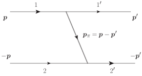
Figure 2: The pion exchange diagram in the $B^{(*)}\bar{B}^{*}$ channels. The solid and dashed line represent a heavy-light meson and the pion, respectively.

In the framework of the Time-Ordered Perturbation Theory (TOPT), the OPE potential acquires two contributions depicted in Fig. 1(a) and (b) where the thin vertical line pinpoints the three-body intermediate state. In Fig. 2, all relevant momenta are shown explicitly for the first ordering TOPT diagram — see Fig. 1(a). Notations for the second diagram depicted in Fig. 1(b) are analogous. Then, the OPE potentials at leading order can be written as Baru:2011rs

$$V_{a}^{nn^{\prime}}(M,{\bm{p}},{\bm{p}}^{\prime}) = -\left(\frac{g_{b}}{2f_{\pi}}\right)^{2}\frac{p_{\pi}^{n}p_{\pi}^{n^{\prime}}}{2E_{\pi}(p_{\pi})[E_{\pi}(p_{\pi})+E_{1^{\prime}}(p^{\prime})+E_{2}(p)-M]},$$ (27)

$$V_{b}^{nn^{\prime}}(M,{\bm{p}},{\bm{p}}^{\prime}) = -\left(\frac{g_{b}}{2f_{\pi}}\right)^{2}\frac{p_{\pi}^{n}p_{\pi}^{n^{\prime}}}{2E_{\pi}(p_{\pi})[E_{\pi}(p_{\pi})+E_{1}(p)+E_{2^{\prime}}(p^{\prime})-M]},$$ (28)

where

$$\displaystyle E_{i}(p)=m_{i}+\frac{p^{2}}{2m_{i}},\quad i=1^{(\prime)},2^{(\prime)},$$

(29)

$$E_{\pi}=\sqrt{\bm{p}_{\pi}^{2}+m_{\pi}^{2}},\quad\bm{p}_{\pi}={\bm{p}}-{\bm{p}}^{\prime},$$

with $M$ being the total energy of the system and $E_{x}$ being the energy of the particle $x$. The incoming and outgoing momenta are denoted as ${\bm{p}}$ and ${\bm{p}}^{\prime}$, and the Cartesian indices $n$ and $n^{\prime}$ contract with either the $B^{*}$ ($\bar{B}^{*}$) polarisation vectors or with the vector product of polarisation vectors, $B^{*}\times\bar{B}^{*}$.

In the presence of pions, no additional coupled-channel transitions but those discussed in Sect. II.1 are possible for the $B^{(*)}\bar{B}^{*}$ systems with the quantum numbers $1^{+-}$. Therefore, using the elastic basis vectors introduced in Sect. II.1 — see Eq. (5) — the OPE potential in this channel can be written as

$$V^{\pi}(M,p,p^{\prime})=\left(\begin{array}[]{cccc}V_{SS}^{\pi 11}&V_{SD}^{\pi 11}&V_{SS}^{\pi 12}&V_{SD}^{\pi 12}\\ V_{DS}^{\pi 11}&V_{DD}^{\pi 11}&V_{DS}^{\pi 12}&V_{DD}^{\pi 12}\\ V_{SS}^{\pi 21}&V_{SD}^{\pi 21}&V_{SS}^{\pi 22}&V_{SD}^{\pi 22}\\ V_{DS}^{\pi 21}&V_{DD}^{\pi 21}&V_{DS}^{\pi 22}&V_{DD}^{\pi 22}\end{array}\right),$$ (34)

where, in each matrix element $V^{\pi\,\lambda\lambda^{\prime}}_{LL^{\prime}}(M,p,p^{\prime})$, the index $\lambda(\lambda^{\prime})=1,2$ labels the particle channel ($B\bar{B}^{*}=1,B^{*}\bar{B}^{*}=2$) and $L(L^{\prime})$ stands for the angular momentum of the state $\lambda(\lambda^{\prime})$. The details of the partial wave decomposition of the OPE can be found in Ref. Baru:2017pvh ; see also Appendix B of Ref. Nieves:2012tt . Then,

$$V_{SS}^{\pi\,\lambda\lambda^{\prime}}(M,p,p^{\prime}) = \frac{g_{b}^{2}}{24f_{\pi}^{2}}\left(\begin{array}[]{cc}1&-2\\ -2&1\end{array}\right)^{\lambda\lambda^{\prime}}\Bigl{[}2pp^{\prime}\Delta_{1}^{\pi\,\lambda\lambda^{\prime}}\left(M,p,p^{\prime}\right)-\left(p^{2}+p^{\prime 2}\right)\Delta_{0}^{\pi\,\lambda\lambda^{\prime}}\left(M,p,p^{\prime}\right)\Bigr{]},$$ (37)

$$V_{SD}^{\pi\,\lambda\lambda^{\prime}}(M,p,p^{\prime}) = \frac{g_{b}^{2}}{24\sqrt{2}f_{\pi}^{2}}\left(\begin{array}[]{cc}1&1\\ 1&1\end{array}\right)^{\lambda\lambda^{\prime}}\Bigl{[}3p^{2}\Delta_{2}^{\pi\,\lambda\lambda^{\prime}}\left(M,p,p^{\prime}\right)-4pp^{\prime}\Delta_{1}^{\pi\,\lambda\lambda^{\prime}}\left(M,p,p^{\prime}\right)+\left(2p^{\prime 2}-p^{2}\right)\Delta_{0}^{\pi\,\lambda\lambda^{\prime}}\left(M,p,p^{\prime}\right)\Bigr{]},$$ (40)

$$V_{DS}^{\pi\,\lambda\lambda^{\prime}}(M,p,p^{\prime}) = V_{SD}^{\pi\,\lambda\lambda^{\prime}}(M,p^{\prime},p),$$

$$V_{DD}^{\pi\,\lambda\lambda^{\prime}}(M,p,p^{\prime}) = \frac{g_{b}^{2}}{24f_{\pi}^{2}}\left[\left(\begin{array}[]{cc}1&0\\ 0&1\end{array}\right)^{\lambda\lambda^{\prime}}V_{1}^{\pi\,\lambda\lambda^{\prime}}\left(M,p,p^{\prime}\right)-\left(\begin{array}[]{cc}0&1\\ 1&0\end{array}\right)^{\lambda\lambda^{\prime}}V_{2}^{\pi\,\lambda\lambda^{\prime}}\left(M,p,p^{\prime}\right)\right],$$ (46)

with

$$V_{1}^{\pi\,\lambda\lambda^{\prime}}\left(M,p,p^{\prime}\right) = \frac{9}{2}pp^{\prime}\Delta_{3}^{\pi\,\lambda\lambda^{\prime}}\left(M,p,p^{\prime}\right)-3\left(p^{2}+p^{\prime 2}\right)\Delta_{2}^{\pi\,\lambda\lambda^{\prime}}\left(M,p,p^{\prime}\right)$$ (47)

$$- \frac{1}{2}pp^{\prime}\Delta_{1}^{\pi\,\lambda\lambda^{\prime}}\left(M,p,p^{\prime}\right)+\left(p^{2}+p^{\prime 2}\right)\Delta_{0}^{\pi\,\lambda\lambda^{\prime}}\left(M,p,p^{\prime}\right),$$

$$V_{2}^{\pi\,\lambda\lambda^{\prime}}\left(M,p,p^{\prime}\right) = \frac{9}{2}pp^{\prime}\Delta_{3}^{\pi\,\lambda\lambda^{\prime}}\left(M,p,p^{\prime}\right)-\frac{3}{2}\left(p^{2}+p^{\prime 2}\right)\Delta_{2}^{\pi\,\lambda\lambda^{\prime}}\left(M,p,p^{\prime}\right)$$ (48)

$$- \frac{5}{2}pp^{\prime}\Delta_{1}^{\pi\,\lambda\lambda^{\prime}}\left(M,p,p^{\prime}\right)+\frac{1}{2}\left(p^{2}+p^{\prime 2}\right)\Delta_{0}^{\pi\,\lambda\lambda^{\prime}}\left(M,p,p^{\prime}\right).$$

The functions $\Delta_{k}^{\pi\,\lambda\lambda^{\prime}}$ ($k=0,1,2,3$) are defined as

$$\Delta_{k}^{\pi\,\lambda\lambda^{\prime}}(M,p,p^{\prime})=\int_{-1}^{1}dx\frac{x^{k}}{2E_{\pi}(p_{\pi})}\Bigl{[}D_{a}^{\pi\,\lambda\lambda^{\prime}}(p,p^{\prime},x)+D_{b}^{\pi\,\lambda\lambda^{\prime}}(p,p^{\prime},x)\Bigr{]},$$ (49)

with the contributions of the two TOPT orderings — see Fig. 1 — given by

$$D_{a}^{\pi\,\lambda\lambda^{\prime}}(p,p^{\prime},x) = \frac{1}{E_{\pi}(p_{\pi})+(E_{1^{\prime}}(p^{\prime})+E_{2}(p))^{\lambda\lambda^{\prime}}-M}$$ (50)

$$= \frac{1}{E_{\pi}(p_{\pi})+(m_{1^{\prime}}+m_{2}+p^{\prime 2}/(2m_{1^{\prime}})+p^{2}/(2m_{2}))^{\lambda\lambda^{\prime}}-M},$$

$$D_{b}^{\pi\,\lambda\lambda^{\prime}}(p,p^{\prime},x) = \frac{1}{E_{\pi}(p_{\pi})+(E_{1}(p)+E_{2^{\prime}}(p^{\prime}))^{\lambda\lambda^{\prime}}-M}$$ (51)

$$= \frac{1}{E_{\pi}(p_{\pi})+(m_{1}+m_{2^{\prime}}+p^{2}/(2m_{1})+p^{\prime 2}/(2m_{2^{\prime}}))^{\lambda\lambda^{\prime}}-M},$$

where $p_{\pi}=\sqrt{p^{2}+p^{\prime 2}-2pp^{\prime}x}$, and the mass matrices for the intermediate particles read

$$m_{1}=m_{2^{\prime}}=\left(\begin{array}[]{cc}m_{B^{*}}&m_{B^{*}}\\ m_{B^{*}}&m_{B^{*}}\end{array}\right),$$ (54)

$$m_{2}=\left(\begin{array}[]{cc}m_{B}&m_{B}\\[-5.69054pt] \\[-5.69054pt] m_{B^{*}}&m_{B^{*}}\end{array}\right),\quad m_{1^{\prime}}=\left(\begin{array}[]{cc}m_{B}&m_{B^{*}}\\ m_{B}&m_{B^{*}}\end{array}\right).$$ (60)

Note that, in the static limit, that is, when the recoil corrections are neglected, the functions $V_{1}^{\pi\,\lambda\lambda^{\prime}}$, $V_{2}^{\pi\,\lambda\lambda^{\prime}}$, and $D_{a}^{\pi\,\lambda\lambda^{\prime}}(p,p^{\prime},x)$, $D_{b}^{\pi\,\lambda\lambda^{\prime}}(p,p^{\prime},x)$ do not depend on the particle-channel indices ($\lambda$ and $\lambda^{\prime}$), so that in this approximation the dependence on the latter comes entirely from the coefficients in Eq. (37).

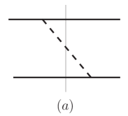
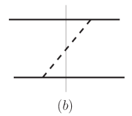
Figure 1: Diagrams in the Time-Ordered Perturbation Theory responsible for the two contributions to the OPE potential. The solid and dashed line represent a heavy-light meson and the pion, respectively.

III Numerical solutions of the coupled-channel Lippmann-Schwinger Equations

With the OPE and OEE interaction included and decomposed in partial waves, the full interaction potential in the elastic channels reads

$$V^{\rm eff}_{\alpha\beta}(M,p,p^{\prime})=V^{\rm CT}_{\alpha\beta}(M,p,p^{\prime}) + V^{\pi}_{\alpha\beta}(M,p,p^{\prime})$$

$$+ V^{\eta}_{\alpha\beta}(M,p,p^{\prime}),$$

where the effects of the inelastic channels are contained in $V^{\rm CT}_{\alpha\beta}(M,p,p^{\prime})$ as given by Eq. (9) and the channel indices are defined by Eqs. (4) and (5).

We work in terms of the production amplitudes rather than the scattering amplitudes which are more convenient given that we aim at fits for the invariant mass distributions measured in the $\Upsilon(10860)$ decays. Thus, the system of the LSEs reads

$$U_{\alpha}(M,p) = F_{\alpha}(M,p)$$

$$- \sum_{\beta}\int U_{\beta}(M,q)G_{\beta}(M,q)V_{\beta\alpha}^{\text{eff}}(M,q,p)\frac{d^{3}q}{(2\pi)^{3}}.$$

Here $F_{\alpha}(M,p)$ and $U_{\alpha}(M,p)$ denote the Born and the physical production amplitude of the $\alpha$-th elastic channel from a point-like source, respectively. We include those source terms in $S$ waves only. Note that a $D$ wave contribution to the source could be re-expressed as an additional energy dependence of the source, which, however, is not required by the data. This is also in line with the results of Ref. Mehen:2013mva from which one concludes that the two-step process $\Upsilon(10860)\to B^{*}B^{(*)}\to B^{*}B^{(*)}\pi$ with the pion emitted from the $B$-meson line, that provides the energy dependence, is suppressed as compared to a point-like source. The Green’s function for a two-heavy-meson intermediate state reads

$$G_{\alpha}(M,q)=\frac{2\mu_{\alpha}}{q^{2}-p_{\alpha}^{2}-i\epsilon},\quad p_{\alpha}^{2}\equiv 2\mu_{\alpha}(M-m_{\rm th}^{\alpha}),$$ (63)

where $m_{\rm th}^{\alpha}$ stands for the $\alpha$-th elastic threshold and $\mu_{\alpha}$ is the reduced mass in the channel $\alpha$. Other components of the multichannel amplitude responsible for the production of the inelastic channels in the final state can be obtained from $U_{\alpha}(M,p)$ algebraically which is a consequence of the omitted direct interactions in the inelastic channels Hanhart:2015cua ; Guo:2016bjq . In particular, for the $i$-th inelastic channel in the final state we have

$$U_{i}(M,p_{i})=-\int\frac{d^{3}q}{(2\pi)^{3}}U_{\alpha}(M,q)G_{\alpha}(M,q)v_{\alpha i}(M,q,p_{i}),$$ (64)

$$p_{i}=\frac{1}{2M}\lambda^{1/2}(M^{2},m_{1i}^{2},m_{2i}^{2}),$$

where $\lambda(m_{1}^{2},m_{2}^{2},m_{3}^{2})$ is the standard triangle function. Expression (64) is based on the assumption that the data are dominated by the $Z_{b}(10610)$ and $Z_{b}(10650)$ poles which emerge from $B^{(*)}\bar{B}^{*}$ dynamics, so that the Born amplitudes $F_{i}(M,p)$ coming from the inelastic sources can be safely neglected. While this is well justified for the $h_{b}(mP)\pi$ channels, since the $Z_{b}$ poles are necessary for the change in the heavy quark spin, it appears to be unjustified for the heavy-spin-conserving $\Upsilon(nS)\pi$ channels. However, to fully control the interplay of the source term and the resonance terms one would need to properly include the $\pi\pi$ interaction which goes beyond the scope of this work. This is why, in what follows, we do not include the line shapes in the $\Upsilon(nS)\pi$ channels into the fit.

In terms of the production amplitudes the expressions for the differential widths in the elastic and inelastic channels read (see Refs. Hanhart:2015cua ; Guo:2016bjq for the derivation)

$$\frac{d\Gamma_{\alpha}}{dM} \equiv y_{\alpha}^{\rm th}(M)=\frac{1}{3}\ \frac{2m_{B^{(*)}}2m_{B^{*}}2m_{\Upsilon(10860)}}{32\pi^{3}m_{\Upsilon(10860)}^{2}}\;p_{\pi}^{*}p_{\alpha}|U_{\alpha}|^{2},$$

$$\frac{d\Gamma_{i}}{dM} \equiv y_{i}^{\rm th}(M)=\frac{1}{3}\ \frac{2m_{h_{i}}2m_{H_{i}}2m_{\Upsilon(10860)}}{32\pi^{3}m_{\Upsilon(10860)}^{2}}\;p_{\pi}^{*}p_{i}|U_{i}|^{2},$$

respectively, where $p_{\pi}^{*}$ is the three-momentum of the spectator pion in the rest frame of the $\Upsilon(10860)$ and $p_{\alpha}(p_{i})$ is the three-momentum in the $\alpha$-th elastic ($i$-th inelastic) channel in the rest frame of the $B^{*}\bar{B}^{(*)}$ ($\Upsilon(nS)\pi/h_{b}(mP)\pi$) system. Then, the total branching in an elastic or inelastic channel $x$ is defined as

$$\mbox{Br}_{x}=\frac{\Gamma_{x}}{\sum_{\alpha=1}^{N_{\text{e}}}\Gamma_{\alpha}+\sum_{i=1}^{N_{\text{in}}}\Gamma_{i}},$$ (66)

where

$$\Gamma_{x}=\int_{M_{\rm min}}^{M_{\rm max}}y_{x}^{\rm th}(M)dM.$$ (67)

For simplicity, we define the branching fractions (BFs) relative to the $B\bar{B}^{*}\pi$ channel,

$$\mbox{BF}_{x}=\frac{\mbox{Br}_{x}}{\mbox{Br}_{B\bar{B}^{*}\pi}}=\frac{\Gamma_{x}}{\Gamma_{B\bar{B}^{*}\pi}}.$$ (68)

The $\chi^{2}$ function to be minimised in the fitting process is built as

$$\chi^{2} = \sum_{\alpha=B^{(*)}\bar{B}^{*}}\sum_{n_{\alpha}}\left(\frac{{\cal N}_{\alpha}y^{\rm th}_{\alpha}(M_{n_{\alpha}})-y^{\rm exp}_{\alpha}(M_{n_{\alpha}})}{\delta_{n_{\alpha}}}\right)^{2}+\left(\frac{\mbox{BF}_{B^{*}\bar{B}^{*}}^{\rm th}-\mbox{BF}_{B^{*}\bar{B}^{*}}^{\rm exp}}{\delta_{{\rm BF}_{B^{*}\bar{B}^{*}}}}\right)^{2}$$

$$+ \sum_{i=h_{b}(mP)\pi}\left\{\sum_{n_{i}}\left(\frac{{\cal N}_{i}y^{\rm th}_{i}(M_{n_{i}})-y^{\rm exp}_{i}(M_{n_{i}})}{\delta_{n_{i}}}\right)^{2}+\left(\frac{\mbox{BF}_{i}^{\rm th}-\mbox{BF}_{i}^{\rm exp}}{\delta_{{\rm BF}_{i}}}\right)^{2}\right\}$$

$$+ \sum_{j=\Upsilon(nS)\pi}\left(\frac{\mbox{BF}_{j}^{\rm th}-\mbox{BF}_{j}^{\rm exp}}{\delta_{{\rm BF}_{j}}}\right)^{2},$$

where $y^{\rm exp}$’s are the experimental distributions given in the form of histograms (the sums in $n$’s run over bins), $\delta$’s denote the errors, and the normalisation factors ${\cal N}_{x}$ are additional (auxiliary) fitting parameters since the data are presented in arbitrary units. Both line shapes and total branchings are used in the fit for the elastic $B^{(*)}\bar{B}^{*}$ and the inelastic $h_{b}\pi$ channels while for the inelastic channels $\Upsilon\pi$ only the total branchings can be used in the one-dimensional analysis.

Since the production proceeds via pion emission from the $\Upsilon(10860)$ bottomonium, the corresponding Born amplitudes are subject to a HQSS constraint similar to the one given in Eq. (7) for the coupling constants, that is, $\xi_{\Upsilon(10860)}\equiv F_{B^{*}\bar{B}^{*}}(M,p)/F_{B\bar{B}^{*}}(M,p)=-1$ Hanhart:2015cua ; Guo:2016bjq . Then, without loss of generality, one can set

$$F_{B\bar{B}^{*}}(M,p)=-F_{B^{*}\bar{B}^{*}}(M,p)=1,$$ (70)

to fix the overall normalisation of the amplitudes which in any case drops out from the branchings and can be absorbed by the unimportant factors ${\cal N}$ in the $\chi^{2}$ function — see Eqs. (66) and (III).

We may now perform the angular integrations in Eq. (LABEL:eq:LSE) to reduce the three-dimensional integral equation to a one-dimensional equation,

$$U_{\alpha}(M,p)=F_{\alpha}(M,p)-\frac{1}{\pi^{2}}\sum_{\beta}\mu_{\beta}\int_{0}^{\infty}\frac{q^{2}U_{\beta}(M,q)V_{\beta\alpha}^{\text{eff}}(M,q,p)}{q^{2}-p_{\beta}^{2}-i\epsilon}dq.$$ (71)

To render the integrals well defined we introduce a sharp ultraviolet cut-off $\Lambda$ which needs to be larger than all typical three-momenta related to the coupled-channel dynamics. Unless stated otherwise, for the results presented below we choose $\Lambda=1$ GeV. The cut-off dependence of our results will be discussed in Sect. IV.2. When the energy goes above the threshold of the intermediate channel $\beta$, the on-shell three-momentum $p_{\beta}$ is real allowing for a singular integrand at $q^{2}=p_{\beta}^{2}$. In this case one subtraction at the point $q=p_{\beta}$ is implemented to stabilise the numerical result,

$$U_{\alpha}(M,p) = F_{\alpha}(M,p)$$ (72)

$$- \frac{1}{\pi^{2}}\sum_{\beta}\mu_{\beta}\int_{0}^{\Lambda}\frac{q^{2}U_{\beta}(M,q)V_{\beta\alpha}^{\text{eff}}(M,q,p)-p_{\beta}^{2}U_{\beta}(M,p_{\beta})V^{\text{eff}}_{\beta\alpha}(M,p_{\beta},p)}{q^{2}-p_{\beta}^{2}-i\epsilon}dq$$

$$- \frac{1}{2\pi^{2}}\sum_{\beta}\mu_{\beta}p_{\beta}U_{\beta}(M,p_{\beta})V_{\beta\alpha}^{\text{eff}}(M,p_{\beta},p)\left(i\pi-\log\left(\frac{\Lambda+p_{\beta}}{\Lambda-p_{\beta}}\right)\right).$$

Since this equation is valid in the whole complex energy plane, it is also used to find the resonance poles in Sect. V.

The masses of particles used in the calculations are Patrignani:2016xqp

$$m_{B}=5279~{}{\rm MeV},$$

$$m_{B^{*}}=5324~{}{\rm MeV},$$

$$m_{\pi}=137.28~{}{\rm MeV},$$

$$m_{\Upsilon(10860)}=10860~{}{\rm MeV},$$

$$m_{\Upsilon(1S)}=9460~{}{\rm MeV},$$ (73)

$$m_{\Upsilon(2S)}=10023~{}{\rm MeV},$$

$$m_{\Upsilon(3S)}=10355.2~{}{\rm MeV},$$

$$m_{h_{b}(1P)}=9898.6~{}{\rm MeV},$$

$$m_{h_{b}(2P)}=10259.8~{}{\rm MeV}.$$

IV Fit schemes and results

In this section we fit the line shapes of the two $Z_{b}$ states in both elastic ($B^{(*)}\bar{B}^{*}$) and inelastic ($h_{b}(mP)\pi$, $m=1,2$) channels. As was already mentioned above, the line shapes in the inelastic $\Upsilon(nS)\pi$ ($n=1,2,3$) channels cannot be included into the fit yet, since the data contain a significant contribution driven by the two-pion final state interaction that we cannot include straightforwardly in the present approach. In addition, the analysis has to be multidimensional. Meanwhile, the partial branchings for all measured elastic and inelastic channels are included in our analysis — see Eq. (III) for the formula for $\chi^{2}$ and Table 1 where the branchings are quoted relative to the $B\bar{B}^{*}\pi$ channel. In the branching fractions the interference terms with crossed channels are effectively included via scaling factors gauged in test calculations. It turns out that those scaling factors are very close to 1 in the $h_{b}\pi$ channels, but are $5\%$, $10\%$, and $20\%$ for the partial BF’s in the $\Upsilon(1S)\pi$, $\Upsilon(2S)\pi$, and $\Upsilon(3S)\pi$ channels, respectively.

BF, %	$B^{*}\bar{B}^{*}\pi$	$\Upsilon(1S)\pi\pi$	$\Upsilon(2S)\pi\pi$	$\Upsilon(3S)\pi\pi$	$h_{b}(1P)\pi\pi$	$h_{b}(2P)\pi\pi$
Exp.	$50\pm 10$	$0.6\pm 0.3$	$4\pm 1$	$2\pm 1$	$9\pm 2$	$15\pm 3$
A	$58.04_{-5.83}^{+6.00}$	$0.55_{-0.24}^{+0.34}$	$3.34_{-1.29}^{+1.76}$	$1.72_{-0.82}^{+1.17}$	$8.25_{-2.37}^{+3.22}$	$11.52_{-3.73}^{+4.73}$
G	$54.13_{-18.07}^{+18.83}$	$0.55_{-0.26}^{+0.41}$	$3.51_{-1.48}^{+2.28}$	$1.83_{-0.95}^{+1.59}$	$9.18_{-2.40}^{+3.59}$	$14.92_{-4.09}^{+6.00}$

Table 1: The branching fractions (BFs), in per cent, for the elastic and inelastic channels in the $\Upsilon(10860)$ decays via the two $Z_{b}$ states relative to the $B\bar{B}^{*}\pi$ channel for which the BF is set to unity Garmash:2014dhx ; Belle:2011aa ; Garmash:2015rfd .

IV.1 The role of pion dynamics, HQSS violation and higher-order interactions

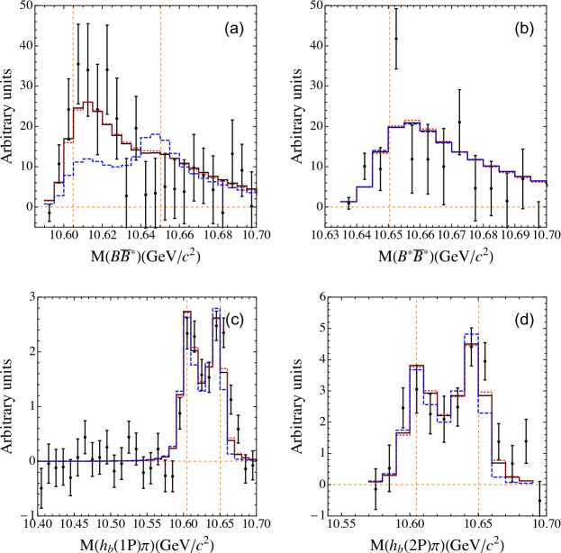
Figure 3: The fitted line shapes for Schemes A (solid black curves), B (red dotted curves) and C (blue dashed curves) in the elastic $B^{(*)}\bar{B}^{*}$ and in the inelastic $h_{b}(mP)\pi$ ($m=1,2$) channels. The vertical dashed orange lines indicate the position of the $B\bar{B}^{*}$ and $B^{*}\bar{B}^{*}$ thresholds. The experimental data are from Refs. Belle:2011aa ; Garmash:2015rfd .

In this section, we investigate the impact of various effects, included in this work for the first time, on the line shapes. To gain a proper insight on the role of these effects, we include them one by one. We, therefore, consider the following different schemes:

• Scheme A: Only the $\mathcal{O}(p^{0})$ $S$-wave contact potentials are considered.

• Scheme B: As Scheme A with OPE added, however, only in $S$ waves.

• Scheme C: As Scheme B, but with $D$-wave OPE included.

• Scheme D: As Scheme C but allowing for a sizeable HQSS violation.

• Scheme E: As Scheme C, but with the $\mathcal{O}(p^{2})$ $\mathcal{D}_{SD}$ contact potential.

• Scheme F: As Scheme C, but with the $\mathcal{O}(p^{2})$ $\mathcal{D}_{d}$, $\mathcal{D}_{f}$, $\mathcal{D}_{SD}$ contact potentials.

• Scheme G: As Scheme F, but with OEE included in addition.

Scheme	$|g_{\Upsilon(1S)}|$	$|g_{\Upsilon(2S)}|$	$|g_{\Upsilon(3S)}|$	$|g_{h_{b}(1P)}|$	$|g_{h_{b}(2P)}|$	$\chi^{2}/\text{d.o.f.}$
A	$0.30\pm 0.07$	$1.01\pm 0.20$	$1.28\pm 0.34$	$3.29\pm 0.38$	$11.38\pm 1.46$	$1.29$
B	$0.31\pm 0.07$	$1.05\pm 0.20$	$1.33\pm 0.35$	$3.19\pm 0.35$	$11.15\pm 1.40$	$1.23$
C	$0.30\pm 0.07$	$1.00\pm 0.20$	$1.22\pm 0.33$	$4.85\pm 0.64$	$16.24\pm 2.54$	$2.00$
D	$0.38\pm 0.55$	$1.35\pm 1.08$	$1.89\pm 0.52$	$3.94\pm 0.52$	$13.87\pm 1.98$	$1.54$
E	$0.30\pm 0.07$	$1.04\pm 0.20$	$1.43\pm 0.36$	$2.76\pm 0.29$	$9.99\pm 1.08$	$0.95$
F	$0.26\pm 0.06$	$0.88\pm 0.17$	$1.16\pm 0.29$	$1.89\pm 0.22$	$6.98\pm 0.81$	$0.83$
G	$0.25\pm 0.06$	$0.88\pm 0.17$	$1.15\pm 0.29$	$1.92\pm 0.22$	$7.07\pm 0.84$	$0.83$

Table 2: The fitted values of the coupling constants for Schemes A-H. The cut-off $\Lambda$ is set to 1 GeV as discussed in the text. The couplings $g_{\Upsilon(nS)}$ ($n=1,2,3$) are given in the units of $\mbox{GeV}^{-2}$ while the couplings $g_{h_{b}(mP)}$ ($m=1,2$) have the dimension of $\mbox{GeV}^{-3}$. Only the absolute values are presented since physical quantities are not sensitive to the couplings’ signs. To demonstrate the quality of each fit we quote the corresponding reduced $\chi^{2}/\text{d.o.f.}$ in the last column.

Scheme	$\mathcal{C}_{d}$	$\mathcal{C}_{f}$	$\mathcal{D}_{d}$	$\mathcal{D}_{SD}$
A	$-3.30\pm 0.11$	$-0.06\pm 0.13$	$0$	$0$
B	$-0.51\pm 0.11$	$-5.64\pm 0.13$	$0$	$0$
C	$0.80\pm 0.14$	$-4.50\pm 0.15$	$0$	$0$
D	$1.22\pm 0.20$	$-4.71\pm 0.21$	$0$	$0$
E	$-0.08\pm 0.30$	$-4.15\pm 0.59$	$0$	$-5.83\pm 0.57$
F	$1.63\pm 0.43$	$-5.28\pm 0.26$	$-2.99\pm 0.58$	$-3.93\pm 0.53$
G	$1.34\pm 0.40$	$-3.95\pm 0.27$	$-3.38\pm 0.54$	$-3.13\pm 0.61$

Table 3: The $\mathcal{O}(p^{0})$ ($\mathcal{C}_{d}$ and $\mathcal{C}_{f}$) and $\mathcal{O}(p^{2})$ ($\mathcal{D}_{d}$ and $\mathcal{D}_{SD}$) contact terms (in the units of $\mathrm{GeV}^{-2}$ and $\mathrm{GeV}^{-4}$, respectively) for each fit scheme. The contact term $\mathcal{D}_{f}$ is set to 0 because it is strongly correlated with $\mathcal{C}_{f}$, does not affect the value of $\chi^{2}/\text{d.o.f.}$ and is, therefore, redundant.

The parameters of the fits for all schemes described above are listed in Tables 2 and  3. In what follows, we discuss the quality of the fits and draw conclusions on the role played by various effects.

The fit results for Schemes A, B and C are shown in Fig. 3 by the solid black, red dotted and blue dashed curves, respectively. The line shapes of Scheme A are basically identical to those based on the parameterisation proposed in Refs. Guo:2016bjq ; Hanhart:2015cua ; Hanhart:2016eyl . In particular, also here the diagonal and off-diagonal matrix elements of the direct interaction potential satisfy the strong inequality $|\mathcal{C}_{f}|\ll|\mathcal{C}_{d}|$ which ensures that the transitions between the two elastic channels are suppressed. It has to be noticed, however, that the parameters in Scheme A of the present paper cannot be directly compared with those from Ref. Guo:2016bjq because of a different regularisation.

Scheme B, with the $S$-wave dynamic OPE included, provides a fit of the same quality as the one in Scheme A. The resulting line shapes are quite similar for both fits which is consistent with the claim made in Ref. Guo:2016bjq on a moderate role played by the OPE. On the contrary, the claim of Ref. Voloshin:2015ypa that already the $S$-wave OPE changes the line shape up to $30\%$ near threshold is not supported by our fit B. It is instructive to identify the most relevant differences between the approaches employed in Ref. Voloshin:2015ypa and in this work: First, the off-diagonal terms connecting the $B\bar{B}^{*}$ with the $B^{*}\bar{B}^{*}$ channel and neglected in Ref. Voloshin:2015ypa turn out to be large in the OPE potential and even exceed the diagonal terms by roughly a factor of 2 — see Eq. (37). Secondly, the argument of Ref. Voloshin:2015ypa is based on a perturbative treatment of the OPE while in this work the pions are treated nonperturbatively and all parameters are re-fitted to the data. Indeed, before drawing conclusions on the role of long-range interactions the short-range part of the OPE, intimately connected to the contact interactions Baru:2015nea , needs to be appropriately renormalised which is achieved in this work by refitting the contact terms to the line shapes. After the re-fit we find that the central $S$-wave OPE can be absorbed to a very large extent into a re-definition of the contact interactions which is in line with the observation made in Ref. Baru:2017gwo .

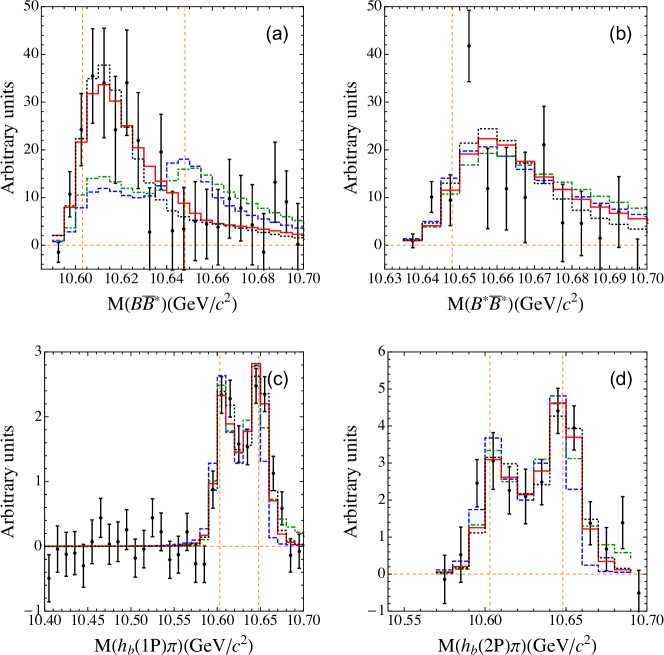
Figure 4: The fitted line shapes for Schemes C (blue dashed curves), D (green dot-dashed curves), E (red solid curves) and G (black dotted curves) in the elastic $B^{(*)}\bar{B}^{*}$ and in the inelastic $h_{b}(mP)\pi$ ($m=1,2$) channels. The experimental data are from Refs. Belle:2011aa ; Garmash:2015rfd .

The fit for Scheme C demonstrates that $D$ waves in the OPE can play a non-negligible role for the line shapes — this is most clearly visible in the $B\bar{B}^{*}$ spectra in Fig. 3 where now a bump appears around the $B^{*}\bar{B}^{*}$ threshold. This result should not come as a surprise given the large momentum scale $p_{\rm typ}$, defined in Eq. (1), introduced by the splitting between the elastic thresholds, which enhances the $D$ waves and, in particular, the contribution from the $S$-$D$ transitions. These findings are in line with the claims made in Refs. Baru:2016iwj ; Baru:2017gwo . Although the fit for Scheme C is essentially consistent with the $B^{*}\bar{B}^{*}$ distribution as well as with the distributions in the inelastic channels, the shape of the $B\bar{B}^{*}$ spectrum distorted by the $D$-wave OPE is not supported by the data. The observation that the experimental line shapes do not exhibit a hump structure around the $B^{*}\bar{B}^{*}$ threshold was related in Ref. Voloshin:2016cgm with a possible existence of the light-quark symmetry in QCD. In what follows, we investigate two different variations of the potential aiming at an improved description of the data.

In Fig. 4 we demonstrate the impact of various higher-order interactions on the line shapes. In particular, in the fit for Scheme D (green dot-dashed curves) we release the HQSS breaking parameters in the elastic and inelastic potentials as well as in the production vertex (that is, $\xi_{\Upsilon(nS)}$, $\xi_{h_{b}(mP)}$ and $\epsilon$) and allow them to deviate up to 50% from the HQSS predicted values. This gives

$$\xi_{\Upsilon(10860)}=-1.23\pm 0.07,$$

$$\xi_{\Upsilon(1S)}=-0.66\pm 0.82,$$

$$\xi_{\Upsilon(2S)}=-0.61\pm 0.52,$$

$$\xi_{\Upsilon(3S)}=-0.50\pm 0.54,$$ (74)

$$\xi_{h_{b}(1P)}=1.50\pm 0.07,$$

$$\xi_{h_{b}(2P)}=1.50\pm 0.63,$$

$$\epsilon=-0.50\pm 0.04.$$

However, in spite of a significant HQSS breaking allowed in the fit, the resulting distribution does not show a qualitative improvement leaving, in particular, the bump structure around the $B^{*}\bar{B}^{*}$ threshold nearly unchanged.

On the other hand, the inclusion of a single ${\cal O}(p^{2})$ contact interaction $\mathcal{D}_{SD}$ between the $S$-wave and $D$-wave elastic channels (Scheme E) improves the fit considerably (see the red solid curves in Fig. 4) yielding $\chi^{2}/\mbox{d.o.f}=0.95$, as given in Table 2. As required by the data, this term is fine-tuned to cancel a large portion of the $S$-$D$ contribution generated by the tensor part of the OPE. Further, the inclusion of the $\mathcal{O}(p^{2})$ counter terms $\mathcal{D}_{d}$ and $\mathcal{D}_{f}$ between the $S$-wave elastic channels in addition to the $\mathcal{D}_{SD}$ term results only in a very minor change in the fit with the $\chi^{2}/\mbox{d.o.f}=0.83$. In addition, we observe that the low-energy constant $\mathcal{D}_{f}$ is by almost 100% correlated with $\mathcal{C}_{f}$, so that by setting $\mathcal{D}_{f}=0$ one gets the fit with almost exactly the same $\chi^{2}/\mbox{d.o.f}$. By adding also the OEE interaction (Scheme G) one obtains results which lie on top of those for Scheme F (see the black dotted curves for Scheme G) in Fig. 4.

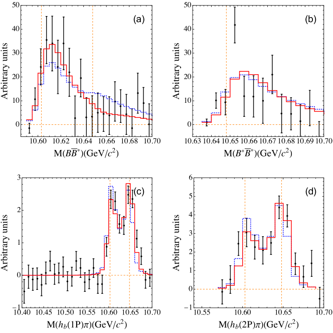
Figure 5: The fitted line shapes for Schemes A (blue dotted curves) and E (red solid curves) in the elastic $B^{(*)}\bar{B}^{*}$ and in the inelastic $h_{b}(mP)\pi$ ($m=1,2$) channels. The experimental data are from Refs. Belle:2011aa ; Garmash:2015rfd .

We are now in a position to re-analyse the net effect from the OPE. In Fig. 5, we compare the results of the fits for Scheme E (red solid curves) with those where pions are switched off (Scheme A — the blue dotted curves). The quantitative improvement that one observes when proceeding from fit A to fit E is related to the residual dynamics from the OPE. Indeed, we checked that the $\mathcal{D}_{SD}$ contact term added to fit A does not improve the quality of the fit. Meanwhile, an attempt to improve the pionless fit A by adding all ${\cal O}(p^{2})$ contact terms with no additional constraints fails: although the quality of the fit improves, the hierarchy of the resulting parameters is very unnatural, because the poles position in this fit is controlled by the NLO ${\cal O}(p^{2})$ terms rather than by the LO ${\cal O}(1)$ ones in conflict with the underlying assumption that higher derivative operators are suppressed. For this reason this fit is not used in what follows. It is important to notice, however, that the EFT expansion is restored once pions are included (fits E, F and G). In particular, the transition from fit E to fits F or G, which corresponds to the addition of the ${\cal O}(p^{2})$ $S$-$S$ contact terms, has a moderate (perturbative) impact on the line shapes as well as the poles.

Finally, in Fig. 6 we present the results for Scheme G including the uncertainties which correspond to a $1\sigma$ deviation in the parameters including correlations.

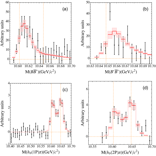
Figure 6: The fitted line shapes for Scheme G with the uncertainties corresponding to a $1\sigma$ deviation in the parameters of the fits. The experimental data are from Refs. Belle:2011aa ; Garmash:2015rfd .

In summary, the results presented in this section demonstrate that

• the data can be equally well described with or without the central $S$-wave OPE potential since the latter can be absorbed into a re-definition of the $S$-wave short-range contact terms;

• the inclusion of $D$ waves affects the line shapes noticeably which confirms the claims found in the literature that $D$ waves are important in the near-threshold charmonium-like and bottomonium-like systems Baru:2016iwj ; Baru:2017gwo . However, the current data call for the promotion of the $\mathcal{O}(p^{2})$ $S$-wave-to-$D$-wave counter term $\mathcal{D}_{SD}$ to lower order and for tuning this term to balance the $S$-$D$ dynamics from the OPE. The residual effect from the OPE on the line shapes is, however, still sizeable:

• the effect of the OEE interaction is negligibly small;

• the data are essentially consistent with HQSS constraints imposed on the potential;

• no indication for the importance of $\mathcal{O}(p^{2})$ contact interactions in the inelastic channels is seen in the data.

IV.2 Dependence of the results on the regulator

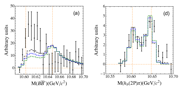
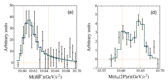
Figure 7: The fitted line shapes for Scheme C (upper panel) and Scheme G (lower panel) in the elastic $B\bar{B}^{*}$ and inelastic $\pi h_{b}(2P)$ channels with sharp cut-offs 800 MeV (black long-dashed), 1000 MeV (blue dashed) and 1200 MeV (green dot-dashed), respectively. The experimental data are from Refs. Belle:2011aa ; Garmash:2015rfd .

In this chapter, we investigate if the promotion of the $S$-$D$ counter term is called for by the renormalisation of the leading order amplitudes. In Fig. 7 we show the regulator dependence of the results corresponding to the fits G and C, that is, those fits with and without the $\mathcal{O}(p^{2})$ contact terms and OEE interactions in addition to the OPE. The results for fit C show a clearly visible cut-off dependence in the $B\bar{B}^{*}$ and $h_{b}(2P)\pi$ channels when the (sharp) cut-off in the LSEs, treated as a hard scale, is varied in a reasonable range from 800 to 1200 MeV (cf. black long-dashed, blue dashed and green dotted-dashed curves). Note that in an effective field theory where a potential, which is then iterated in a scattering equation, is expanded in terms of a given expansion parameter one cannot expect a complete regulator independence of observable quantities at a given order. This implies that the regulator should not be chosen too large and that regulator effects of sub-leading order are common. It is, therefore, difficult to judge, if the mentioned variations call for an additional counter term at LO or not. However, it is certainly interesting to observe that for the same cut-off variation the curves in fit G (as well as in fit F) remain unchanged indicating that the theory is fully renormalised. The same pattern is observed in the other channels which are therefore not shown.

V The poles position and the nature of the $Z_{b}$ states

In this section we discuss the extraction of the poles of the amplitude in the complex plane. In general, in order to search for the poles in a multi-channel problem a multi-sheet Riemann surface in the complex energy plane needs to be invoked. However, we consider the four-sheet Riemann surface corresponding to the two elastic channels only, because all inelastic thresholds are remote and their impact on the poles of interest, which are located near the elastic thresholds, is expected to be minor. Then, for two coupled channels with the thresholds split by the mass difference $\delta$, the four-sheeted Riemann surface can be mapped onto a single-sheeted plane of a variable which is traditionally denoted as $\omega$ kato and which, for a given energy $E=M-m_{B}-m_{B^{*}}$, is defined via

$$\displaystyle k_{1}=\sqrt{\frac{\mu_{1}\delta}{2}}\left(\omega+\frac{1}{\omega}\right),~{}k_{2}=\sqrt{\frac{\mu_{2}\delta}{2}}\left(\omega-\frac{1}{\omega}\right),$$

(75)

$$\displaystyle E=\frac{k_{1}^{2}}{2\mu_{1}}=\frac{k_{2}^{2}}{2\mu_{2}}+\delta=\frac{\delta}{4}\left(\omega^{2}+\frac{1}{\omega^{2}}+2\right),$$

where $\mu_{1}$ and $\mu_{2}$ are the reduced masses in the first ($B\bar{B}^{*}$) and in the second ($B^{*}\bar{B}^{*}$) elastic channel, respectively. Then the one-to-one correspondence between the four Riemann sheets in the $E$-plane (denoted as RS-N, where N=I, II, III, IV) and various regions in the $\omega$-plane reads

$$\mbox{RS-I}: \quad{\rm Im}~{}k_{1}>0,\quad{\rm Im}~{}k_{2}>0,$$

$$\mbox{RS-II}: \quad{\rm Im}~{}k_{1}<0,\quad{\rm Im}~{}k_{2}>0,$$

$$\mbox{RS-III}: \quad{\rm Im}~{}k_{1}<0,\quad{\rm Im}~{}k_{2}<0,$$

$$\mbox{RS-IV}: \quad{\rm Im}~{}k_{1}>0,\quad{\rm Im}~{}k_{2}<0.$$

The corresponding regions in the $\omega$-plane are depicted in the first plot in Fig. 8. The thick solid line corresponds to the real values of the energy lying on RS-I. It is easy to see that the physical region between the two thresholds corresponds to $|\omega|=1$, with both Re$(\omega)$ and Im$(\omega)$ positive, and the thresholds at $E=0$ and $E=\delta$ are mapped to the points $\omega=\pm i$ and $\omega=\pm 1$, respectively. The inelastic channels in the energy plane are interpreted as one additional effective remote channel with the momentum $k_{\rm in}$ and, in order to find all relevant poles, both possibilities with ${\rm Im}~{}k_{\rm in}>0$ and ${\rm Im}~{}k_{\rm in}<0$ are considered. As it is now effectively a three-channel problem, the number of Riemann sheets doubles and so does the number of poles representing the physics for each state. Hence, each pole has now its mirror partner located on a different sheet of the eight-sheeted Riemann surface but corresponding to the same physical state.

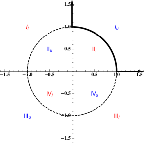
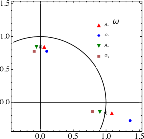
Figure 8: Left panel: The unitary-cut-free complex $\omega$-plane for the two elastic channels, $B\bar{B}^{*}$ and $B^{*}\bar{B}^{*}$, obtained from the four-Riemann-sheet complex energy plane by the conformal transformation (75). The eight regions separated by the unit circle and by the two axes correspond to the upper and lower half-planes [see the subscripts $u$ and $l$] in the four Riemann sheets of the energy plane denoted as RS-N with N=I, II, III, IV kato ; Dudek:2016cru . The bold line indicates the physical region of a real energy $E$ kato . Right panel: The poles position in the complex $\omega$ plane for the fit Schemes A and G described in the text. Only the poles closest to the physical region are given while the distant poles are not shown. The red triangle ($A_{-}$) and blue circle ($G_{-}$) stand for the poles for the fit Schemes A and G, respectively, with all the inelastic channels on their unphysical (${\rm Im}~{}k_{\rm in}<0$) Riemann sheets. The green inverted triangle ($A_{+}$) and pink box ($G_{+}$) are for the poles for the fit Schemes A and G, respectively, with all the inelastic channels on their physical (${\rm Im}~{}k_{\rm in}>0$) Riemann sheets. The crosses stand for the poles for fit A when all inelastic channels are switched off.

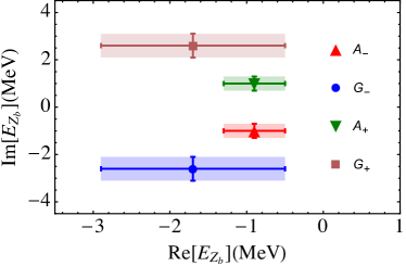
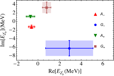
Figure 9: The real and the imaginary part of the $Z_{b}$ (left panel) and $Z_{b}^{\prime}$ (right panel) poles [see the definition in Eq. (76)] for fit Schemes A and G. For the notation of poles see Fig. 8.

The poles position in the $\omega$-plane for the fit Schemes A and G from the previous section is shown in the right panel of Fig. 8. As long as the inelastic channels are switched off, one is back to the two-channel problem with one relevant pole corresponding to each state. For example, the poles for the fit Scheme A but without inelastic channels are shown by the crosses (x) in Fig. 8: the cross on the imaginary axis on RS-II (close to $\omega=i$) corresponds to a virtual $B\bar{B}^{*}$ state pole associated with the $Z_{b}$ state while the other pole, residing on RS-IV (close to $\omega=1$), represents the physics related to the $Z_{b}^{\prime}$ — it is a virtual state in the $B^{*}\bar{B}^{*}$ channel slightly shifted to the complex plane due to coupled-channel effects. When the effective inelastic channel is on, one arrives at a pair of poles for each state: one for ${\rm Im}~{}k_{\rm in}>0$ and one for ${\rm Im}~{}k_{\rm in}<0$ — the corresponding solutions are labeled by “$+$” and “$-$”, respectively. For the $Z_{b}$, the two resulting poles on RS-II₊ and RS-II_- are symmetric with respect to the imaginary axis in the omega plane which results in complex-conjugate solutions for the energies (see Table 4). Unlike the $Z_{b}$, the poles for the $Z_{b}^{\prime}$ on RS-III_- and RS-IV₊ are slightly asymmetric due to coupled-channel effects. In any case, it is apparent that the poles obtained in the full calculation, including inelastic channels, reside in the vicinity of those found without inelastic channels, that implies that the role played by the inelastic channels is sub-leading in line with a molecular interpretation of the $Z_{b}$ states.

The corresponding energies evaluated relative to the relevant elastic threshold,

$$E_{Z_{b}}=M_{Z_{b}}^{\rm pole}-m_{B}-m_{B^{*}},\quad E_{Z_{b}^{\prime}}=M_{Z_{b}^{\prime}}^{\rm pole}-2m_{B^{*}},$$ (76)

are listed in Table 4 and are visualised in Figs. 8 and 9 (the errors in the poles position corresponds to a $1\sigma$ deviation for the whole parameter list). Note that the sign convention is such that positive energies refer to above-thresholds poles — see definition (76).

scheme	$E_{Z_{b}}(\mathrm{MeV})$	$E_{Z_{b}^{\prime}}(\mathrm{MeV})$
$A_{-}$	$(-0.9\pm 0.4)-i(1.0\pm 0.3)$	$(-0.6\pm 0.3)-i(1.2\pm 0.4)$
$G_{-}$	$(-1.7\pm 1.2)-i(2.6\pm 0.5)$	$(2.9\pm 2.3)-i(6.2\pm 1.8)$
$A_{+}$	$(-0.9\pm 0.4)+i(1.0\pm 0.3)$	$(-0.7\pm 0.4)+i(1.2\pm 0.3)$
$G_{+}$	$(-1.7\pm 1.2)+i(2.6\pm 0.5)$	$(0.8\pm 0.4)+i(3.3\pm 1.3)$

Table 4: The energies $E_{Z_{b}}$ and $E_{Z_{b}^{\prime}}$ (see the definition in Eq. (76)) for the fit Schemes A and G. The energies denoted as $A_{-}$ and $G_{-}$ stand for the poles for the fit Schemes A and G, respectively, with all the inelastic channels on their unphysical (${\rm Im}~{}k_{\rm in}<0$) Riemann sheets. The energies denoted as $A_{+}$ and $G_{+}$ are for the poles for the fit Schemes A and G, respectively, with all the inelastic channels on their physical (${\rm Im}~{}k_{\rm in}>0$) Riemann sheets. The errors correspond to a $1\sigma$ deviation in the fitted parameters.

The two poles for Fit A representing the results based on S-wave contact interactions (shown as an up- (red) and down-pointing (green) triangles in Figs. 8 and 9) are essentially consistent with those obtained in Ref. Guo:2016bjq — see Fig. 8 of the quoted paper. As one can see from Table 4 and from Figs. 8 and 9, the inclusion of the OEE and especially the OPE and ${\cal O}(p^{2})$ contact interactions in Fit G changes the poles position to some extent but all the poles reside in the vicinity of the corresponding thresholds. This result is consistent with the expectation that the line shapes are controlled predominantly by the poles position. Indeed, although the parameters of fits A and one of our best fits (fit G) are very different (see Tables 2 and 3), fit G provides a better but still comparable description of the data as fit A, as one can see from the line shapes shown in Fig. 5 and from the values of $\chi^{2}/\mbox{d.o.f.}$ quoted in Table 2. Thus, both fits describe the $Z_{b}$ state as a shallow virtual state located below the $B\bar{B}^{*}$ threshold. Meanwhile, the $Z_{b}^{\prime}$ state is consistent with both a virtual state and an above-threshold resonance interpretation, with the latter option preferred by the pionful fits (like fit G).

VI Summary

This work continues a series of papers aimed at a systematic description of the line shapes of near-threshold resonances in general and, in particular, at understanding the nature and properties of the $Z_{b}^{\pm}(10610)$ and $Z_{b}^{\pm}(10650)$ states in the spectrum of bottomonium. Unlike the previous papers in the series Hanhart:2015cua ; Guo:2016bjq , in this work, we do not resort to an analytic parameterisation for the line shapes but rely on an EFT approach to calculate the line shapes explicitly. In particular, in order to obtain the production and scattering amplitudes, we construct the effective potential to leading order in the chiral and heavy quark expansion and iterate it to all orders employing coupled-channel Lippmann-Schwinger equations. This allows us to verify the accuracy of the practical parameterisation suggested in Ref. Hanhart:2015cua and to estimate the role played by the $\pi$- and $\eta$-exchanges, which cannot be straightforwardly incorporated into the scheme of Refs. Hanhart:2015cua ; Guo:2016bjq because of their non-separable form.

The results of this work can be summarised as follows:

• We find that the distributions obtained from the direct numerical solution of the LSEs with just S-wave contact potentials provide a nearly identical description of the data to that achieved using the parameterisation derived in Refs. Guo:2016bjq ; Hanhart:2015cua ; Hanhart:2016eyl .

• We include the OPE interaction on top of the contact potentials in the elastic channels and demonstrate that the inclusion of the $S$-wave OPE affects the line shapes only marginally. After a re-fit to the data required to appropriately renormalise the short-range interactions, basically the whole $S$-wave OPE contribution can be absorbed to a re-definition of the $S$-wave contact interactions. Therefore, we do not support the claim of Ref. Voloshin:2015ypa that OPE changes the line shape of near threshold states by about 30%.

• For the actual value of the splitting of the two elastic thresholds, $\delta\approx 45$ MeV, the momentum scale $p_{\rm typ}\simeq 500$ MeV which controls the coupled-channel ($B\bar{B}^{*}$-$B^{*}\bar{B}^{*}$) dynamics is relatively large — see Eq. (1). For such momenta, the role played by the OPE in $D$ waves turns out to be significant even after a re-fit, so that one cannot neglect this effect in order to extract the resonance parameters with a sufficiently high accuracy. However, the resulting significant distortion of the line shapes from the OPE is not supported by the currently available experimental data in the $B\bar{B}^{*}$ channel: Indeed, a clear bump structure around the $B^{*}\bar{B}^{*}$ threshold unavoidably generated by the $S$-$D$ OPE transitions is not seen in the most recent data. In order to cure this, we include the additional contact term allowed by heavy quark symmetry and chiral symmetry at order $\mathcal{O}(p^{2})$ to find that the resulting line shapes are in a very good agreement with the data, with a reduced $\chi^{2}/\text{d.o.f.}$ around unity. The role played by various $\mathcal{O}(p^{2})$ contact interactions is different: on the one hand, the single contact term which contributes to the $S$-to-$D$-wave transitions absorbs a large part of the $S$-$D$ OPE piece and, in addition, brings an additional residual contribution — both effects together improve the quality of the fit considerably; on the other hand, two allowed $S$-$S$ contact interactions play a sub-leading role resulting only in a marginal change in the fits. Finally, we conclude that after the inclusion of the $\mathcal{O}(p^{2})$ contact interactions the residual effect from the OPE moderate.

• There are indications that the inclusion of the $S$-$D$ contact term at leading order is required by renormalisation. However, to make this statement more sound a complete calculation to next-to-leading order would be necessary. Since this would come with additional parameters that need to be fixed by data, we postpone this effort until improved data become available.

• We find that the data are consistent with HQSS symmetry constraints imposed on the potential.

• The data do not call for the inclusion of $\mathcal{O}(p^{2})$ contact interactions in the elastic-to-inelastic transitions.

• The effect from the $\eta$-exchange potential is negligible.

• We extract the position of the poles responsible for the $Z_{b}^{\pm}(10610)$ and $Z_{b}^{\pm}(10650)$ and find them to reside on the unphysical Riemann sheets just below ($Z_{b}$) or just above ($Z_{b}^{\prime}$) the corresponding elastic threshold.

Before closing, we would like to stress that the observed strong cancellation between the OPE and the additional ${\cal O}(p^{2})$ $S$-$D$ contact terms is very puzzling. The pion plays a very special role in QCD due to its intimate connection to the spontaneous breaking of chiral symmetry. In addition, since the $D^{*}D\pi$ coupling is known (see Eq. (26)), the OPE comes without adjustable parameters. Still, data demand a very large cancellation of this part of the potential. Whether or not this cancellation is accidental in the system at hand or if it has deeper reasons in QCD calls for further studies which, however, go beyond the scope of this work. Clearly, more accurate experimental data for the $Z_{b}$’s, especially in the elastic channels, and, hopefully, new data for their spin partner states would be of great relevance and importance for such studies.

In conclusion, the results presented provide a good understanding of the line shapes with the $\chi^{2}$/d.o.f. $\simeq 1$ for the best fit. Given stability of the results to various higher-order interactions included and the quality of the fits, it is unlikely that higher-order contributions not included explicitly in the current study, such as two-pion exchange contributions at next-to-leading order, affect the conclusions of the analysis. As a consequence, the LECs extracted from the presented fits can be used to make predictions for the molecular spin-partner states within the same theoretical framework and without introducing any additional parameters spinpartners . It remains to be seen if the strong cancellation of the one-pion exchange and the short-range contributions, which takes place for the $Z_{b}$’s, persists also for their spin partners.

Appendix A Effective Lagrangians

The effective Lagrangian describing isovector $B^{(*)}\bar{B}^{(*)}$ scattering at low energies reads

$${\cal L}={\rm Tr}\left[H^{\dagger}_{a}\left(i\partial_{0}+\frac{\bm{\nabla}^{2}}{2M}\right)_{ba}H_{b}\right]+\frac{\Delta}{4}{\rm Tr}[H^{\dagger}_{a}\sigma^{i}H_{a}\sigma^{i}]$$

$$+{\rm Tr}\left[\bar{H}^{\dagger}_{a}\left(i\partial_{0}+\frac{\bm{\nabla}^{2}}{2M}\right)_{ab}\bar{H}_{b}\right]+\frac{\Delta}{4}{\rm Tr}[\bar{H}^{\dagger}_{a}\sigma^{i}\bar{H}_{a}\sigma^{i}]$$

$$-\frac{C_{10}}{8}{\rm Tr}[\bar{H}^{\dagger}_{a}\tau^{A}_{aa^{\prime}}H^{\dagger}_{a^{\prime}}H_{b}\tau_{bb^{\prime}}^{A}\bar{H}_{b^{\prime}}]-\frac{C_{11}}{8}{\rm Tr}[\bar{H}^{\dagger}_{a}\tau^{A}_{aa^{\prime}}\sigma^{i}H^{\dagger}_{a^{\prime}}H_{b}\tau_{bb^{\prime}}^{A}\sigma^{i}\bar{H}_{b^{\prime}}]$$

$$-\frac{D_{10}}{8}\left\{{\rm Tr}[\nabla^{i}\bar{H}^{\dagger}_{a}\tau^{A}_{aa^{\prime}}\nabla^{i}H^{\dagger}_{a^{\prime}}H_{b}\tau_{bb^{\prime}}^{A}\bar{H}_{b^{\prime}}+{\rm Tr}[\bar{H}^{\dagger}_{a}\tau^{A}_{aa^{\prime}}H^{\dagger}_{a^{\prime}}\nabla^{i}H_{b}\tau_{bb^{\prime}}^{A}\nabla^{i}\bar{H}_{b^{\prime}}]\right\}$$ (77)

$$-\frac{D_{11}}{8}\left\{{\rm Tr}[\nabla^{i}\bar{H}^{\dagger}_{a}\tau^{A}_{aa^{\prime}}\sigma^{j}\nabla^{i}H^{\dagger}_{a^{\prime}}H_{b}\tau_{bb^{\prime}}^{A}\sigma^{j}\bar{H}_{b^{\prime}}+{\rm Tr}[\bar{H}^{\dagger}_{a}\tau^{A}_{aa^{\prime}}\sigma^{j}H^{\dagger}_{a^{\prime}}\nabla^{i}H_{b}\tau_{bb^{\prime}}^{A}\sigma^{j}\nabla^{i}\bar{H}_{b^{\prime}}]\right\}$$

$$-\frac{D_{12}}{8}\left\{{\rm Tr}[(\nabla^{i}\bar{H}^{\dagger}_{a}\tau^{A}_{aa^{\prime}}\sigma^{i}\nabla^{j}H^{\dagger}_{a^{\prime}}+\nabla^{j}\bar{H}^{\dagger}_{a}\tau^{A}_{aa^{\prime}}\sigma^{i}\nabla^{i}H^{\dagger}_{a^{\prime}}-\frac{2}{3}\delta^{ij}\nabla^{k}\bar{H}^{\dagger}_{a}\tau^{A}_{aa^{\prime}}\sigma^{i}\nabla^{k}H^{\dagger}_{a^{\prime}})H_{b}\tau_{bb^{\prime}}^{A}\sigma^{j}\bar{H}_{b^{\prime}}]\right.$$

$$+\left.{\rm Tr}[\bar{H}^{\dagger}_{a}\tau^{A}_{aa^{\prime}}\sigma^{i}H^{\dagger}_{a^{\prime}}(\nabla^{i}H_{b}\tau_{bb^{\prime}}^{A}\sigma^{j}\nabla^{j}\bar{H}_{b^{\prime}}+\nabla^{j}H_{b}\tau_{bb^{\prime}}^{A}\sigma^{j}\nabla^{i}\bar{H}_{b^{\prime}}-\frac{2}{3}\delta^{ij}\nabla^{k}H_{b}\tau_{bb^{\prime}}^{A}\sigma^{j}\nabla^{k}\bar{H}_{b^{\prime}})]\right\},$$

where the terms in the first row in Eq. (77) stand for the leading heavy hadron chiral perturbation theory Lagrangian of Refs. Wise:1992hn ; Burdman:1992gh ; Yan:1992gz , written in the two-component notation of Ref. Hu:2005gf . The terms in the second row represent the Lagrangian for anti-heavy mesons. The heavy mesons and anti-heavy mesons interact via the remaining terms in the Lagrangian: the third row in Eq. (77) corresponds to $O(p^{0})$ $S$-wave contact interactions Mehen:2011yh ; AlFiky:2005jd , while the last three rows represent the ${\cal O}(p^{2})$ contact terms with two derivatives. The contact terms $\propto D_{10}$ and $D_{11}$ contribute to $S$-wave interactions while the last term $\propto D_{12}$ is projected out to give rise to the $S$-$D$ transitions. Since we are only interested in the $S$-$S$ and $S$-$D$ transitions for the $B^{(*)}\bar{B}^{(*)}$ scattering, all the terms of the kind $\propto\nabla^{i}H^{\dagger}\nabla^{j}H$ contributing to $P$ waves were dropped. We also note here that the expansion in spatial derivatives employed in the Lagrangian (77) yields contributions to four-point vertices rather than to two-point vertices and propagators. This expansion is controlled by the scale provided by the range of forces (for example, by the mass of the lightest $t$-channel exchange particle and not by the heavy-quark mass), so that arbitrary coefficients $D$ in front of the terms with derivatives do not violate the reparametrisation invariance discussed in detail in Ref. Luke:1992cs .

In Eq. (77) $H_{a}=P_{a}+V_{a}^{i}\sigma^{i}$ stands for the heavy meson superfield combining a pseudoscalar ($P_{a}$) and a vector ($V_{a}$) meson, $a$ and $b$ are $SU(2)$ isospin indices, and the isospin matrices are normalised via the trace as $\tau^{A}_{ab}\tau^{B}_{ba}=2\delta^{AB}$.

The charge and Hermitian conjugate operators for the superfield $H_{a}$ read

$$\bar{H}_{a}=\sigma_{2}\mathcal{C}H_{a}^{T}\mathcal{C}^{-1}\sigma_{2}=\bar{P}_{a}-\bar{V}_{a}^{i}\sigma^{i},\quad H_{a}^{\dagger}=P_{a}^{\dagger}+V_{a}^{i\dagger}\sigma^{i},\quad\bar{H}_{a}^{\dagger}=\bar{P}_{a}^{\dagger}-\bar{V}_{a}^{i\dagger}\sigma^{i},$$ (78)

and they transform as

$$H_{a}\stackrel{{\scriptstyle\mathcal{P}}}{{\longrightarrow}}-H_{a},\quad H_{a}\stackrel{{\scriptstyle\mathcal{C}}}{{\rightarrow}}\sigma_{2}\bar{H}_{a}^{T}\sigma_{2},\quad H_{a}\stackrel{{\scriptstyle\mathcal{S}}}{{\rightarrow}}SH_{a},\quad H_{a}\stackrel{{\scriptstyle\mathcal{U}}}{{\rightarrow}}H_{b}U_{ba}^{\dagger},$$

$$\quad\bar{H}_{a}\stackrel{{\scriptstyle\mathcal{P}}}{{\longrightarrow}}-\bar{H}_{a},\quad\bar{H}_{a}\stackrel{{\scriptstyle\mathcal{C}}}{{\rightarrow}}\sigma_{2}H_{a}^{T}\sigma_{2},\quad\bar{H}_{a}\stackrel{{\scriptstyle\mathcal{S}}}{{\rightarrow}}\bar{H}_{a}\bar{S}^{\dagger},\quad\bar{H}_{a}\stackrel{{\scriptstyle\mathcal{U}}}{{\rightarrow}}U_{ab}\bar{H}_{b}$$ (79)

under the parity ($\mathcal{P}$), charge ($\mathcal{C}$), heavy-quark spin ($\mathcal{S}$), and chiral ($\mathcal{U}$) transformation. The isoscalar contributions in Lagrangian (77) can be easily restored if one makes a replacement of the isospin Pauli matrices by the corresponding Kronecker delta symbols, that is, for example, $\tau_{ab}\to\delta_{ab}$.

Deriving the Feynman rules from the interaction part of Lagrangian (77) one readily obtains the effective potential given in Eq. (20), where

$$\mathcal{C}_{d}=\displaystyle-C_{11}-C_{10},\quad\mathcal{C}_{f}=C_{10}-C_{11},$$

$$\mathcal{D}_{d}=\displaystyle-D_{11}-D_{10},\quad\mathcal{D}_{f}=D_{10}-D_{11},$$

$$\mathcal{D}_{SD}=\displaystyle\frac{2\sqrt{2}}{3}D_{12}.$$

Appendix B Scaling of higher partial waves in elastic-to-inelastic transitions

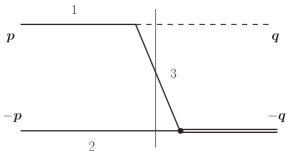
Figure 10: Diagram underlying the transitions from an elastic to an inelastic channel. Solid, dashed and double line denote $B^{(*)}$ mesons, the pion and a heavy quarkonium, respectively. The thin vertical line indicates the time slice of relevance for the discussion.

To understand a possible role of the $D$ waves in the transitions from an elastic to an inelastic channel one needs to study the diagram shown in Fig. 10. Taken as a time-ordered diagram it gives for the intermediate state pinpointed by the thin vertical line

$$G^{-1}_{\rm trans.}(M,{\bm{p}},\bm{q})=E_{\pi}(q)+\left(m_{3}+\frac{({\bm{p}}-\bm{q})^{2}}{2m_{3}}\right)+\left(m_{2}+\frac{{\bm{p}}^{2}}{2m_{2}}\right)-M.$$ (81)

Since the energy region of interest is located near the $Z_{b}$’s states, it is sufficient for the argument to estimate the on-shell transition potential which calls for the substitution $M=m_{1}+m_{2}+{\bm{p}}^{2}/(2\mu)$, where $\mu=m_{1}m_{2}/(m_{1}+m_{2})$ denotes the reduced mass. As an example (but without loss of generality for the argument), we now set $m_{1}=m_{B^{*}}$ and $m_{2}=m_{B}$ that implies $m_{3}=m_{B}$ and $p$ ranges from 0, at the $B\bar{B}^{*}$ threshold, to $p\sim p_{\rm typ}$ (defined in Eq. (1)), when the $B^{*}\bar{B}^{*}$ threshold is approached. Then we get

$$G^{-1}_{\rm trans.}(M,{\bm{p}},\bm{q})=E_{\pi}(q)+\frac{pq}{m_{B}}x+\frac{q^{2}}{2m_{B}}-\delta,$$ (82)

where $x=\cos(\hat{{\bm{p}}{\bm{q}}})$ and tiny corrections $\propto\delta\,p^{2}_{\rm typ}/2m_{B}$ were neglected. It is the term $\propto x$ that eventually supports higher partial waves in the elastic channel. Then the $D$ waves are suppressed relative to the $S$ waves by the factor

$$\left(\frac{p_{\rm typ}}{m_{B}}\right)^{2}\left(\frac{q}{E_{\pi}(q)+q^{2}/(2m_{B})-\delta}\right)^{2}.$$ (83)

The values of $q$ range from about 200 MeV, for the transition to the $\Upsilon(3S)\pi$ channel, to 1.1 GeV, for the transition to the $\Upsilon(1S)\pi$ channel. It is easy to verify that, for such values of $q$, the second factor in Eq. (83) is close to unity, that provides a justification for the estimate used in the main text — see the discussion above Eq. (6).

Appendix C Flavour symmetry and the pseudoscalar exchange potentials

In this appendix we discuss the pseudoscalar exchange potential between the heavy mesons. For definiteness, we stick to the $B\bar{B}^{*}$ channel as to an example. The flavour projector for a pseudoscalar ($P$ or $\bar{P}$) and a vector ($\bar{V}$ or $V$) for the $1^{+-}$ quantum numbers reads

$$\mathcal{P}_{B\bar{B^{*}}}(1^{+-})=\frac{1}{2}\left(P\tau^{A}\bar{V}-V\tau^{A}\bar{P}\right),$$ (84)

where the overall factor 1/2 ensures the proper normalisation of the projectors,

$$\mathcal{P}_{B\bar{B^{*}}}(1^{+-})^{\dagger}\mathcal{P}_{B\bar{B^{*}}}(1^{+-}) = \frac{1}{4}{\rm Tr}\left[\left(\bar{V}^{\dagger}\tau^{A}{P}^{\dagger}-\bar{P}^{\dagger}\tau^{A}V^{\dagger}\right)\left(P\tau^{B}\bar{V}-V\tau^{B}\bar{P}\right)\right]=\frac{1}{4}{\rm Tr}\left(2\tau^{A}\tau^{B}\right)=\delta^{AB}.$$

Here, like in Appendix A, the standard normalisation for the isospin matrices was used, ${\rm Tr}[\tau^{A}\tau^{B}]=2\delta^{AB}$.

Then, the flavour factor involving isospin and C-parity for the OPE diagram can be evaluated as

$$\frac{1}{4}{\rm Tr}\left[\left(\bar{V}^{\dagger}\tau^{A}{P}^{\dagger}-\bar{P}^{\dagger}\tau^{A}V^{\dagger}\right)\left(P^{\dagger}\tau^{a}V\right)\left(V\tau^{B}\bar{P}-P\tau^{B}\bar{V}\right)\left(\bar{V}^{\dagger}\tau^{a}\bar{P}\right)\right]$$

$$+ \frac{1}{4}{\rm Tr}\left[\left(\bar{V}^{\dagger}\tau^{A}{P}^{\dagger}-\bar{P}^{\dagger}\tau^{A}V^{\dagger}\right)\left(V^{\dagger}\tau^{a}P\right)\left(V\tau^{B}\bar{P}-P\tau^{B}\bar{V}\right)\left(\bar{P}^{\dagger}\tau^{a}\bar{V}\right)\right]$$

$$= \frac{1}{4}{\rm Tr}\left(-\tau^{A}\tau^{a}\tau^{B}\tau^{a}-\tau^{A}\tau^{a}\tau^{B}\tau^{a}\right)=\delta^{AB},$$

where at the last step above an easily verified relation

$${\rm Tr}\left[\tau^{A}\tau^{a}\tau^{B}\tau^{a}\right]=-2\delta^{AB}$$ (86)

was used. It is this part of the calculation which makes difference between the OPE and OEE potentials. Indeed, in the latter case the trace takes the form

$${\rm Tr}\left[\tau^{A}\hat{1}\tau^{B}\hat{1}\right]=2\delta^{AB},$$ (87)

where the unit matrices correspond to the $\eta$ emission/absorption vertices which substitute the Pauli matrices from the pion vertices — see Eq. (86).

Finally, considering an additional factor $1/\sqrt{3}$ which comes from the 8-th Gell-Mann matrix for the $SU(3)$ group — see Eq. (23) — and which, therefore, enters each $\eta$-vertex, one arrives at the following list of changes needed to proceed from the OPE potential to the OEE one: (i) the flavour factor +1, for the OPE in the isovector channel, should be replaced by $-1$, for the OEE; (ii) the pion mass $m_{\pi}$ should be replaced by the $\eta$ mass $m_{\eta}$, and (iii) the pion coupling constant $g_{b}$ should be replaced by the $\eta$ coupling constant $g_{b}/\sqrt{3}$.

Interestingly, if the flavour symmetry group $SU(3)$ is extended to $U(3)$ then the potentials from the $\pi$-, $\eta$-, and $\eta^{\prime}$-exchange cancel each other identically in the strict flavour symmetry limit Aceti:2014kja . However, because of the $U(1)$ anomaly, there are no reasons to expect the $\eta^{\prime}$ to possess properties of the Goldstone boson DiVecchia:1980yfw ; Rosenzweig:1979ay ; Kawarabayashi:1980dp ; Witten:1980sp .

References

- (1) A. Bondar et al. [Belle Collaboration], Phys. Rev. Lett. 108, 122001 (2012).
- (2) M. Ablikim et al. [BESIII Collaboration], Phys. Rev. Lett. 110, 252001 (2013).
- (3) Z. Q. Liu et al. [Belle Collaboration], Phys. Rev. Lett. 110, 252002 (2013).
- (4) M. Ablikim et al. [BESIII Collaboration], Phys. Rev. Lett. 111, 242001 (2013).
- (5) S. K. Choi et al. [Belle Collaboration], Phys. Rev. Lett. 100, 142001 (2008).
- (6) R. Mizuk et al. [Belle Collaboration], Phys. Rev. D 80, 031104 (2009).
- (7) K. Chilikin et al. [Belle Collaboration], Phys. Rev. D 88, 074026 (2013).
- (8) R. Aaij et al. [LHCb Collaboration], Phys. Rev. Lett. 112, 222002 (2014).
- (9) I. Adachi [Belle Collaboration], arXiv:1105.4583 [hep-ex].
- (10) I. Adachi et al. [Belle Collaboration], arXiv:1209.6450 [hep-ex].
- (11) A. Garmash et al. [Belle Collaboration], Phys. Rev. Lett. 116, 212001 (2016).
- (12) A. Ali, C. Hambrock and W. Wang, Phys. Rev. D 85, 054011 (2012).
- (13) A. Esposito, A. L. Guerrieri, F. Piccinini, A. Pilloni and A. D. Polosa, Int. J. Mod. Phys. A 30, 1530002 (2015).
- (14) L. Maiani, A. D. Polosa and V. Riquer, Phys. Lett. B 778, 247 (2018).
- (15) A. E. Bondar, A. Garmash, A. I. Milstein, R. Mizuk and M. B. Voloshin, Phys. Rev. D 84, 054010 (2011).
- (16) M. Cleven, F. K. Guo, C. Hanhart and U.-G. Meißner, Eur. Phys. J. A 47, 120 (2011).
- (17) J. Nieves and M. P. Valderrama, Phys. Rev. D 84, 056015 (2011).
- (18) J. R. Zhang, M. Zhong and M. Q. Huang, Phys. Lett. B 704, 312 (2011).
- (19) Y. Yang, J. Ping, C. Deng and H. S. Zong, J. Phys. G 39, 105001 (2012).
- (20) Z. F. Sun, J. He, X. Liu, Z. G. Luo and S. L. Zhu, Phys. Rev. D 84, 054002 (2011).
- (21) S. Ohkoda, Y. Yamaguchi, S. Yasui, K. Sudoh and A. Hosaka, Phys. Rev. D 86, 014004 (2012).
- (22) M. T. Li, W. L. Wang, Y. B. Dong and Z. Y. Zhang, J. Phys. G 40, 015003 (2013).
- (23) H. W. Ke, X. Q. Li, Y. L. Shi, G. L. Wang and X. H. Yuan, JHEP 1204, 056 (2012).
- (24) J. M. Dias, F. Aceti and E. Oset, Phys. Rev. D 91, 076001 (2015).
- (25) E. S. Swanson, Phys. Rev. D 91, 034009 (2015).
- (26) F. K. Guo, C. Hanhart, Q. Wang and Q. Zhao, Phys. Rev. D 91, 051504 (2015).
- (27) C. Hanhart, Y. S. Kalashnikova, P. Matuschek, R. V. Mizuk, A. V. Nefediev and Q. Wang, Phys. Rev. Lett. 115, 202001 (2015).
- (28) F.-K. Guo, C. Hanhart, Y. S. Kalashnikova, P. Matuschek, R. V. Mizuk, A. V. Nefediev, Q. Wang and J.-L. Wynen, Phys. Rev. D 93, 074031 (2016).
- (29) M. B. Voloshin, Phys. Rev. D 84, 031502 (2011).
- (30) S. Ohkoda, Y. Yamaguchi, S. Yasui and A. Hosaka, Phys. Rev. D 86, 117502 (2012).
- (31) X. Li and M. B. Voloshin, Phys. Rev. D 86, 077502 (2012).
- (32) M. Cleven, Q. Wang, F. K. Guo, C. Hanhart, U.-G. Meißner and Q. Zhao, Phys. Rev. D 87, 074006 (2013).
- (33) Y. Dong, A. Faessler, T. Gutsche and V. E. Lyubovitskij, J. Phys. G 40, 015002 (2013).
- (34) G. Li, F. l. Shao, C. W. Zhao and Q. Zhao, Phys. Rev. D 87, 034020 (2013).
- (35) S. Ohkoda, S. Yasui and A. Hosaka, Phys. Rev. D 89, 074029 (2014).
- (36) D. Y. Chen, X. Liu and S. L. Zhu, Phys. Rev. D 84, 074016 (2011).
- (37) Y. H. Chen, J. T. Daub, F. K. Guo, B. Kubis, U.-G. Meißner and B. S. Zou, Phys. Rev. D 93, 034030 (2016)
- (38) Y. H. Chen, M. Cleven, J. T. Daub, F. K. Guo, C. Hanhart, B. Kubis, U.-G. Meißner and B. S. Zou, Phys. Rev. D 95, 034022 (2017).
- (39) T. Mehen and J. W. Powell, Phys. Rev. D 84, 114013 (2011).
- (40) M. P. Valderrama, Phys. Rev. D 85, 114037 (2012).
- (41) C. Hidalgo-Duque, J. Nieves and M. P. Valderrama, Phys. Rev. D 87, 076006 (2013).
- (42) J. Nieves and M. P. Valderrama, Phys. Rev. D 86, 056004 (2012).
- (43) F. K. Guo, C. Hidalgo-Duque, J. Nieves and M. P. Valderrama, Phys. Rev. D 88, 054007 (2013).
- (44) M. Karliner and J. L. Rosner, Phys. Rev. Lett. 115, 122001 (2015).
- (45) V. Baru, E. Epelbaum, A. A. Filin, C. Hanhart and A. V. Nefediev, JHEP 1706, 158 (2017).
- (46) X. W. Kang, Z. H. Guo and J. A. Oller, Phys. Rev. D 94, 014012 (2016).
- (47) A. V. Nefediev, Phys. Atom. Nucl. 80, no. 5, 1006 (2017).
- (48) Z. G. Wang and T. Huang, Eur. Phys. J. C 74, 2891 (2014).
- (49) Z. G. Wang, Eur. Phys. J. C 74, 2963 (2014).
- (50) S. S. Agaev, K. Azizi and H. Sundu, Eur. Phys. J. C 77, 836 (2017).
- (51) E. Wilbring, H.-W. Hammer and U.-G. Meißner, arXiv:1705.06176 [hep-ph].
- (52) F. K. Guo, C. Hanhart, U.-G. Meißner, Q. Wang, Q. Zhao and B. S. Zou, Rev. Mod. Phys. 90, 015004 (2018).
- (53) M. B. Voloshin and L. B. Okun, JETP Lett. 23, 333 (1976) [Pisma Zh. Eksp. Teor. Fiz. 23, 369 (1976)].
- (54) N. A. Tornqvist, Phys. Rev. Lett. 67, 556 (1991).
- (55) N. A. Tornqvist, Z. Phys. C 61, 525 (1994).
- (56) Y. R. Liu, X. Liu, W. Z. Deng and S. L. Zhu, Eur. Phys. J. C 56, 63 (2008).
- (57) C. E. Thomas and F. E. Close, Phys. Rev. D 78, 034007 (2008).
- (58) M. Suzuki, Phys. Rev. D 72, 114013 (2005).
- (59) Y. S. Kalashnikova and A. V. Nefediev, Pisma Zh. Eksp. Teor. Fiz. 97, 76 (2013) [JETP Lett. 97, 70 (2013)].
- (60) A. A. Filin, A. Romanov, V. Baru, C. Hanhart, Y. S. Kalashnikova, A. E. Kudryavtsev, U.-G. Meißner and A. V. Nefediev, Phys. Rev. Lett. 105, 019101 (2010).
- (61) V. Baru, E. Epelbaum, A. A. Filin, F.-K. Guo, H.-W. Hammer, C. Hanhart, U.-G. Meißner and A. V. Nefediev, Phys. Rev. D 91, 034002 (2015).
- (62) M. B. Voloshin, Phys. Lett. B 579, 316 (2004).
- (63) S. Fleming, M. Kusunoki, T. Mehen and U. van Kolck, Phys. Rev. D 76, 034006 (2007).
- (64) V. Baru, A. A. Filin, C. Hanhart, Y. S. Kalashnikova, A. E. Kudryavtsev and A. V. Nefediev, Phys. Rev. D 84, 074029 (2011).
- (65) V. Baru, E. Epelbaum, A. A. Filin, C. Hanhart, U.-G. Meißner and A. V. Nefediev, Phys. Lett. B 763, 20 (2016).
- (66) S. Fleming, T. Mehen and I. W. Stewart, Nucl. Phys. A 677, 313 (2000).
- (67) M. Albaladejo, F.-K. Guo, C. Hidalgo-Duque, J. Nieves and M. P. Valderrama, Eur. Phys. J. C 75, 547 (2015).
- (68) M. B. Voloshin, Phys. Rev. D 92, 114003 (2015).
- (69) F. Aceti, M. Bayar, J. M. Dias and E. Oset, Eur. Phys. J. A 50, 103 (2014).
- (70) E. Epelbaum, H. W. Hammer and U.-G. Meißner, Rev. Mod. Phys. 81, 1773 (2009).
- (71) C. Hanhart, Y. S. Kalashnikova, P. Matuschek, R. V. Mizuk, A. V. Nefediev and Q. Wang, J. Phys. Conf. Ser. 675, 022016 (2016).
- (72) M. T. AlFiky, F. Gabbiani and A. A. Petrov, Phys. Lett. B 640, 238 (2006).
- (73) M. Tanabashi et al. [Particle Data Group], Phys. Rev. D 98, 030001 (2018).
- (74) F. Bernardoni et al. [ALPHA Collaboration], Phys. Lett. B 740, 278 (2015).
- (75) B. Grinstein, E. E. Jenkins, A. V. Manohar, M. J. Savage and M. B. Wise, Nucl. Phys. B 380, 369 (1992).
- (76) V. Baru, E. Epelbaum, A. A. Filin, C. Hanhart and A. V. Nefediev, EPJ Web Conf. 137, 06002 (2017).
- (77) T. Mehen and J. Powell, Phys. Rev. D 88, 034017 (2013).
- (78) A. Garmash et al. [Belle Collaboration], Phys. Rev. D 91, 072003 (2015).
- (79) M. B. Voloshin, Phys. Rev. D 93, 074011 (2016).
- (80) M. Kato, Annals Phys. 31, 130 (1965).
- (81) J. J. Dudek et al. [Hadron Spectrum Collaboration], Phys. Rev. D 93, 094506 (2016).
- (82) V. Baru, A. A. Filin, C. Hanhart, A. V. Nefediev, and Q. Wang, in preparation.
- (83) M. B. Wise, Phys. Rev. D 45, R2188 (1992).
- (84) G. Burdman and J. F. Donoghue, Phys. Lett. B 280, 287 (1992).
- (85) T. M. Yan, H. Y. Cheng, C. Y. Cheung, G. L. Lin, Y. C. Lin and H. L. Yu, Phys. Rev. D 46, 1148 (1992) Erratum: [Phys. Rev. D 55, 5851 (1997)].
- (86) J. Hu and T. Mehen, Phys. Rev. D 73, 054003 (2006).
- (87) M. E. Luke and A. V. Manohar, Phys. Lett. B 286, 348 (1992).
- (88) P. Di Vecchia and G. Veneziano, Nucl. Phys. B 171, 253 (1980).
- (89) C. Rosenzweig, J. Schechter and C. G. Trahern, Phys. Rev. D 21, 3388 (1980).
- (90) K. Kawarabayashi and N. Ohta, Nucl. Phys. B 175, 477 (1980).
- (91) E. Witten, Annals Phys. 128, 363 (1980).