Abstract

In this article, we distinguish the charge conjunctions of the interpolating currents, calculate the contributions of the vacuum condensates up to dimension-10 in a consistent way in the operator product expansion, study the masses and pole residues of the $J^{PC}=1^{+\pm}$ hidden charmed tetraquark states with the QCD sum rules, and explore the energy scale dependence in details for the first time. The predictions $M_{X}=3.87^{+0.09}_{-0.09}\,\rm{GeV}$ and $M_{Z}=3.91^{+0.11}_{-0.09}\,\rm{GeV}$ support assigning the $X(3872)$ and $Z_{c}(3900)$ (or $Z_{c}(3885)$) as the $1^{++}$ and $1^{+-}$ diquark-antidiquark type tetraquark states, respectively.

PACS number: 12.39.Mk, 12.38.Lg

Key words: Tetraquark state, QCD sum rules

1 Introduction

There are many candidates with the quantum numbers $J^{PC}=0^{++}$ below $2\,\rm{GeV}$, which cannot be accommodated in one $\bar{q}q$ nonet. The lowest scalar nonet mesons $f_{0}(600)$, $a_{0}(980)$, $K^{*}_{0}(800)$, $f_{0}(980)$ are usually taken as the tetraquark states [1], and have been studied as the diquark-antidiquark type tetraquark states with the QCD sum rules [2]. The QCD sum rules is a powerful theoretical tool in studying the ground state hadrons [3, 4]. For the light tetraquark states, it is difficult to satisfy the two criteria of the QCD sum rules:

$\bullet$ Pole dominance at the phenomenological side;

$\bullet$ Convergence of the operator product expansion [5].
For the hidden (or doubly) charmed (or bottom) tetraquark states (or molecular states), it is more easy to satisfy the two criteria.

In 2003, the Belle collaboration observed a narrow charmonium-like state $X(3872)$ in the $\pi^{+}\pi^{-}J/\psi$ mass spectrum in the exclusive decay processes $B^{\pm}\to K^{\pm}\pi^{+}\pi^{-}J/\psi$ [6]. The evidences for the decay modes $X(3872)\to\gamma J/\psi,\,\gamma\psi^{\prime}$ imply the positive charge conjunction $C=+$ [7]. Angular correlations between final state particles in the $\pi^{+}\pi^{-}J/\psi$ favor the $J^{PC}=1^{++}$ assignment [8]. L. Maiani et al tentatively identify the $X(3872)$ as the $J^{PC}=1^{++}$ tetraquark state with the symmetric spin distribution $[cq]_{S=1}[\bar{c}\bar{q}]_{S=0}+[cq]_{S=0}[\bar{c}\bar{q}]_{S=1}$ [9]. For other possible assignments, one can consult the reviews [10]. In Ref.[11], R. D. Matheus et al take the $X(3872)$ as the $J^{PC}=1^{++}$ diquark-antidiquark type tetraquark state, and study its mass with the QCD sum rules by taking the vacuum condensates up to dimension-8 in the operator product expansion. Thereafter the hidden charmed (or bottom) and doubly open charmed (or bottom) diquark-antidiquark type tetraquark states have been studied extensively with the QCD sum rules [12, 13, 14, 15]. For some articles on the QCD sum rules for the hidden charmed (or bottom) molecular states, one can consult the reviews [16].

In 2013, the BESIII collaboration studied the process $e^{+}e^{-}\to\pi^{+}\pi^{-}J/\psi$ at a center-of-mass energy of 4.260 GeV using a $525\,\rm{pb}^{-1}$ data sample collected with the BESIII detector, and observed a structure $Z_{c}(3900)$ in the $\pi^{\pm}J/\psi$ mass spectrum with a mass of $(3899.0\pm 3.6\pm 4.9)\,\rm{MeV}$ and a width of $(46\pm 10\pm 20)\,\rm{MeV}$ [17]. Then the structure $Z_{c}(3900)$ was confirmed by the Belle and CLEO collaborations [18, 19]. R. Faccini et al tentatively identify the $Z_{c}(3900)$ as the negative charge conjunction partner of the $X(3872)$ [20], other assignments, such as molecular state [21], tetraquark state [22], hadro-charmonium [23], rescattering effect [24], are also suggested. C. F. Qiao and L. Tang studied the $J^{PC}=1^{+-}$ hidden charmed tetraquark state with the QCD sum rules by taking the vacuum condensates up to dimension-8 in the operator product expansion, and obtained the mass $M_{Z}=(3912^{+106}_{-103})\,\rm{MeV}$ [15].

Recently, the BESIII collaboration studied the process $e^{+}e^{-}\to\pi D\bar{D}^{*}$ at $\sqrt{s}=4.26\,\rm{GeV}$ using a $525\,\rm{pb}^{-1}$ data sample collected with the BESIII detector at the BEPCII storage ring, and observed a distinct charged structure $Z_{c}(3885)$ in the $(D\bar{D}^{*})^{\pm}$ invariant mass distribution [25]. The measured mass and width are $(3883.9\pm 1.5\pm 4.2)\,\rm{MeV}$ and $(24.8\pm 3.3\pm 11.0)\,\rm{MeV}$, respectively, and the angular distribution of the $\pi Z_{c}(3885)$ system favors a $J^{P}=1^{+}$ assignment [25]. We tentatively identify the $Z_{c}(3900)$ and $Z_{c}(3885)$ as the same particle according to the uncertainties of the masses and widths. The $1^{+}$ hidden charmed tetraquark states can decay to both the $D\bar{D}^{*}$ and $\pi J/\psi$ final states.

In the QCD sum rules for the hidden charmed (or bottom) tetraquark states and molecular states, the integrals

$$\int_{4m_{Q}^{2}}^{s_{0}}ds\rho_{QCD}(s)\exp\left(-\frac{s}{T^{2}}\right)\,,$$ (1)

are sensitive to the heavy quark masses $m_{Q}$, where the $\rho_{QCD}(s)$ denotes the QCD spectral densities and the $T^{2}$ denotes the Borel parameters. Variations of the heavy quark masses lead to changes of integral ranges $4m_{Q}^{2}-s_{0}$ of the variable $\bf{ds}$ besides the QCD spectral densities, therefore changes of the Borel windows and predicted masses and pole residues. In calculations, we observe that small variations of the heavy quark masses $m_{Q}$ can lead to rather large changes of the predictions [13, 14, 26]. In previous works, the $\overline{MS}$ masses are taken, however, the energy scales at which the QCD spectral densities are calculated are either not shown explicitly (or not specified) [11, 12, 15] or shown explicitly at a special value [13, 14, 26], the energy scale dependence is not studied in details.

In previous works [14], we have studied the axial-vector hidden charmed and hidden bottom tetraquark states with the QCD sum rules, the charge conjunctions are not distinguished. In this article, we distinguish the charge conjunctions of the interpolating currents, calculate the contributions of the vacuum condensates up to dimension-10 in a consistent way in the operator product expansion and discard the perturbative corrections, study the masses and pole residues of the axial-vector hidden charmed tetraquark states, and explore the energy scale dependence in details, and make tentative assignments of the $X(3872)$ and $Z_{c}(3900)$ (or $Z_{c}(3885)$). In Refs.[11, 14, 15], some higher dimension vacuum condensates are neglected. The higher dimension vacuum condensates play an important role in determining the Borel windows, although they maybe play a less important role in the Borel windows. Different Borel windows lead to different ground state masses and pole residues.

The mass is a fundamental parameter in describing a hadron. In order to identify the $X(3872)$ and $Z_{c}(3900)$ (or $Z_{c}(3885)$) as the $J^{PC}=1^{++}$ and $1^{+-}$ hidden charmed tetraquark states, respectively, we must prove that their masses lie in the region $(3.8-4.0)\,\rm{GeV}$ in a consistent way, and there exists a small energy gap between the $C=+$ and $-$ axial-vector tetraquark states.

The article is arranged as follows: we derive the QCD sum rules for the masses and pole residues of the axial-vector tetraquark states in section 2; in section 3, we present the numerical results and discussions; section 4 is reserved for our conclusion.

2 QCD sum rules for the $J^{PC}=1^{+\pm}$ tetraquark states

In the following, we write down the two-point correlation functions $\Pi_{\mu\nu}(p)$ in the QCD sum rules,

$$\Pi_{\mu\nu}(p) = i\int d^{4}xe^{ip\cdot x}\langle 0|T\left\{J_{\mu}(x)J_{\nu}^{\dagger}(0)\right\}|0\rangle\,,$$ (2)

$$J_{\mu}(x) = \frac{\epsilon^{ijk}\epsilon^{imn}}{\sqrt{2}}\left\{u^{j}(x)C\gamma_{5}c^{k}(x)\bar{d}^{m}(x)\gamma_{\mu}C\bar{c}^{n}(x)+tu^{j}(x)C\gamma_{\mu}c^{k}(x)\bar{d}^{m}(x)\gamma_{5}C\bar{c}^{n}(x)\right\}\,,$$ (3)

$t=\pm 1$ denote the positive and negative charge conjunctions, respectively, the $i$, $j$, $k$, $m$, $n$ are color indexes, the $C$ is the charge conjunction matrix. We choose the currents $J_{\mu}(x)$ to interpolate the $J^{PC}=1^{+\pm}$ diquark-antidiquark type tetraquark states $X(3872)$ (to be more precise, the charged partner of the $X(3872)$) and $Z_{c}(3900)$ (or $Z_{c}(3885)$), respectively. Under charge conjunction transform $\widehat{C}$, the currents $J_{\mu}(x)$ have the properties,

$$\widehat{C}J_{\mu}(x)\widehat{C}^{-1} = \pm J_{\mu}(x)\,\,\,\,{\rm for}\,\,\,\,t=\pm 1\,,$$ (4)

which originate from the charge conjunction properties of the scalar and axial-vector diquark states,

$$\widehat{C}\left[\epsilon^{ijk}q^{j}C\gamma_{5}c^{k}\right]\widehat{C}^{-1} = \epsilon^{ijk}\bar{q}^{j}\gamma_{5}C\bar{c}^{k}\,,$$

$$\widehat{C}\left[\epsilon^{ijk}q^{j}C\gamma_{\mu}c^{k}\right]\widehat{C}^{-1} = \epsilon^{ijk}\bar{q}^{j}\gamma_{\mu}C\bar{c}^{k}\,.$$ (5)

We can insert a complete set of intermediate hadronic states with the same quantum numbers as the current operators $J_{\mu}(x)$ into the correlation functions $\Pi_{\mu\nu}(p)$ to obtain the hadronic representation [3, 4]. After isolating the ground state contributions from the pole terms, which are supposed to be tetraquark states $X(3872)$ and $Z_{c}(3900)$ (or $Z_{c}(3885)$), we get the following results,

$$\Pi_{\mu\nu}(p) = \frac{\lambda_{X/Z}^{2}}{M_{X/Z}^{2}-p^{2}}\left(-g_{\mu\nu}+\frac{p_{\mu}p_{\nu}}{p^{2}}\right)+\cdots\,\,,$$ (6)

where the pole residues (or couplings) $\lambda_{X/Z}$ are defined by

$$\langle 0|J_{\mu}(0)|X/Z(p)\rangle=\lambda_{X/Z}\,\varepsilon_{\mu}\,,$$ (7)

the $\varepsilon_{\mu}$ are the polarization vectors of the axial-vector mesons $X(3872)$ and $Z_{c}(3900)$ (or $Z_{c}(3885)$).

The currents $J_{\mu}(x)$ have non-vanishing couplings with the scattering states $DD^{\ast}$, $J/\psi\pi$, $J/\psi\rho$, etc [27]. In the following, we study the contributions of the intermediate meson-loops to the correlation functions $\Pi_{\mu\nu}(p)$,

$$\Pi_{\mu\nu}(p) = -\frac{\widehat{\lambda}_{X/Z}^{2}}{p^{2}-\widehat{M}_{X/Z}^{2}}\widetilde{g}_{\mu\nu}(p)-\frac{\widehat{\lambda}_{X/Z}}{p^{2}-\widehat{M}_{X/Z}^{2}}\widetilde{g}_{\mu\alpha}(p)\Sigma_{DD^{*}}(p)\widetilde{g}^{\alpha\beta}(p)\widetilde{g}_{\beta\nu}(p)\frac{\widehat{\lambda}_{X/Z}}{p^{2}-\widehat{M}_{X/Z}^{2}}$$ (8)

$$-\frac{\widehat{\lambda}_{X/Z}}{p^{2}-\widehat{M}_{X/Z}^{2}}\widetilde{g}_{\mu\alpha}(p)\Sigma_{J/\psi\pi}(p)\widetilde{g}^{\alpha\beta}(p)\widetilde{g}_{\beta\nu}(p)\frac{\widehat{\lambda}_{X/Z}}{p^{2}-\widehat{M}_{X/Z}^{2}}$$

$$-\frac{\widehat{\lambda}_{X/Z}}{p^{2}-\widehat{M}_{X/Z}^{2}}\widetilde{g}_{\mu\alpha}(p)\Sigma_{J/\psi\rho}^{\alpha\beta}(p)\widetilde{g}_{\beta\nu}(p)\frac{\widehat{\lambda}_{X/Z}}{p^{2}-\widehat{M}_{X/Z}^{2}}+\cdots\,,$$

$$= -\frac{\widehat{\lambda}_{X/Z}^{2}}{p^{2}-\widehat{M}_{X/Z}^{2}-\Sigma_{DD^{*}}(p)-\Sigma_{J/\psi\pi}(p)-\Sigma_{J/\psi\rho}(p)+\cdots}\widetilde{g}_{\mu\nu}(p)+\cdots\,,$$

where

$$\Sigma_{DD^{*}}(p) = i\int~{}{d^{4}q\over(2\pi)^{4}}\frac{G^{2}_{X/ZDD^{*}}}{\left[q^{2}-M_{D}^{2}\right]\left[(p-q)^{2}-M_{D^{*}}^{2}\right]}\,,$$ (9)

$$\Sigma_{J/\psi\pi}(p) = i\int~{}{d^{4}q\over(2\pi)^{4}}\frac{G^{2}_{X/ZJ/\psi\pi}}{\left[q^{2}-M_{J/\psi}^{2}\right]\left[(p-q)^{2}-M_{\pi}^{2}\right]}\,,$$ (10)

$$\Sigma_{J/\psi\rho}^{\alpha\beta}(p) = i\int~{}{d^{4}q\over(2\pi)^{4}}\frac{G^{2}_{X/ZJ/\psi\rho}\epsilon^{\alpha\theta\sigma\tau}\epsilon^{\beta\theta^{\prime}\sigma^{\prime}\tau^{\prime}}p_{\tau}p_{\tau^{\prime}}\widetilde{g}_{\theta\theta^{\prime}}(q)\widetilde{g}_{\sigma\sigma^{\prime}}(p-q)}{\left[q^{2}-M_{J/\psi}^{2}\right]\left[(p-q)^{2}-M_{\rho}^{2}\right]}\,,$$ (11)

$$= \Sigma_{J/\psi\rho}(p)\widetilde{g}^{\alpha\beta}(p)+\Sigma_{J/\psi\rho}^{1}(p)\frac{p^{\alpha}p^{\beta}}{p^{2}}\,,$$

$\widetilde{g}_{\mu\nu}(p)=-g_{\mu\nu}+\frac{p_{\mu}p_{\nu}}{p^{2}}$, the $G_{X/ZDD^{*}}$, $G_{X/ZJ/\psi\pi}$, $G_{X/ZJ/\psi\rho}$ are hadronic coupling constants, the $\widehat{\lambda}_{X/Z}$ and $\widehat{M}_{X/Z}$ are bare quantities to absorb the divergences in the self-energies $\Sigma_{DD^{*}}(p)$, $\Sigma_{J/\psi\pi}(p)$, $\Sigma_{J/\psi\rho}(p)$, etc. The renormalized self-energies contribute a finite imaginary part to modify the dispersion relation,

$$\Pi_{\mu\nu}(p) = -\frac{\lambda_{X/Z}^{2}}{p^{2}-M_{X/Z}^{2}+i\sqrt{p^{2}}\Gamma(p^{2})}\widetilde{g}_{\mu\nu}(p)+\cdots\,,$$ (12)

the physical widths $\Gamma_{Z_{c}(3900)}(M_{Z}^{2})=(46\pm 10\pm 20)\,\rm{MeV}$ and $\Gamma_{X(3872)}(M_{X}^{2})<1.2\,\rm{MeV}$ are small enough, the zero width approximation in the hadronic spectral densities works.

The contaminations of the intermediate meson-loops are expected to be small, we take a single pole approximation and approximate the continuum contributions as

$$\int_{4m_{c}^{2}}^{\infty}ds\,\frac{1}{s-p^{2}}\rho_{QCD}(s)\Theta(s-s_{0})\,,$$ (13)

the $\rho_{QCD}(s)$ denotes the full QCD spectral densities; the pole term embodies the net effects. Onset of the continuum states is not abrupt, the ground state, the first excited state, the second excited state, etc, the continuum states appear sequentially. The threshold parameter $s_{0}$ is postponed to large value, where the spectral densities can be well approximated by the contributions of the asymptotic quarks and gluons, in other words, the perturbative contributions. If only the ground state is taken, the $s_{0}$ is not large enough to warrant that the hadronic spectral densities above the $s_{0}$ can be approximated by the perturbative contributions, the $\rho_{QCD}(s)$ should include the contributions of the vacuum condensates besides the perturbative terms.

In the following, we briefly outline the operator product expansion for the correlation functions $\Pi_{\mu\nu}(p)$ in perturbative QCD . We contract the quark fields in the correlation functions $\Pi_{\mu\nu}(p)$ with Wick theorem, obtain the results:

$$\Pi_{\mu\nu}(p) = -\frac{i\epsilon^{ijk}\epsilon^{imn}\epsilon^{i^{\prime}j^{\prime}k^{\prime}}\epsilon^{i^{\prime}m^{\prime}n^{\prime}}}{2}\int d^{4}xe^{ip\cdot x}$$ (14)

$$\left\{{\rm Tr}\left[\gamma_{5}C^{kk^{\prime}}(x)\gamma_{5}CU^{jj^{\prime}T}(x)C\right]{\rm Tr}\left[\gamma_{\nu}C^{n^{\prime}n}(-x)\gamma_{\mu}CD^{m^{\prime}mT}(-x)C\right]\right.$$

$$+{\rm Tr}\left[\gamma_{\mu}C^{kk^{\prime}}(x)\gamma_{\nu}CU^{jj^{\prime}T}(x)C\right]{\rm Tr}\left[\gamma_{5}C^{n^{\prime}n}(-x)\gamma_{5}CD^{m^{\prime}mT}(-x)C\right]$$

$$\mp{\rm Tr}\left[\gamma_{\mu}C^{kk^{\prime}}(x)\gamma_{5}CU^{jj^{\prime}T}(x)C\right]{\rm Tr}\left[\gamma_{\nu}C^{n^{\prime}n}(-x)\gamma_{5}CD^{m^{\prime}mT}(-x)C\right]$$

$$\left.\mp{\rm Tr}\left[\gamma_{5}C^{kk^{\prime}}(x)\gamma_{\nu}CU^{jj^{\prime}T}(x)C\right]{\rm Tr}\left[\gamma_{5}C^{n^{\prime}n}(-x)\gamma_{\mu}CD^{m^{\prime}mT}(-x)C\right]\right\}\,,$$

where the $\mp$ correspond the positive and negative charge conjunctions, respectively, the $U_{ij}(x)$, $D_{ij}(x)$ and $C_{ij}(x)$ are the full $u$, $d$ and $c$ quark propagators, respectively (the $U_{ij}(x)$ and $D_{ij}(x)$ can be written as $S_{ij}(x)$ for simplicity),

$$S_{ij}(x) = \frac{i\delta_{ij}\!\not\!{x}}{2\pi^{2}x^{4}}-\frac{\delta_{ij}\langle\bar{q}q\rangle}{12}-\frac{\delta_{ij}x^{2}\langle\bar{q}g_{s}\sigma Gq\rangle}{192}-\frac{ig_{s}G^{a}_{\alpha\beta}t^{a}_{ij}\left(\!\not\!{x}\sigma^{\alpha\beta}+\sigma^{\alpha\beta}\!\not\!{x}\right)}{32\pi^{2}x^{2}}-\frac{i\delta_{ij}x^{2}\!\not\!{x}g_{s}^{2}\langle\bar{q}q\rangle^{2}}{7776}$$ (15)

$$-\frac{\delta_{ij}x^{4}\langle\bar{q}q\rangle\langle g_{s}^{2}GG\rangle}{27648}-\frac{1}{8}\langle\bar{q}_{j}\sigma^{\mu\nu}q_{i}\rangle\sigma_{\mu\nu}-\frac{1}{4}\langle\bar{q}_{j}\gamma^{\mu}q_{i}\rangle\gamma_{\mu}+\cdots\,,$$

$$C_{ij}(x) = \frac{i}{(2\pi)^{4}}\int d^{4}ke^{-ik\cdot x}\left\{\frac{\delta_{ij}}{\!\not\!{k}-m_{c}}-\frac{g_{s}G^{n}_{\alpha\beta}t^{n}_{ij}}{4}\frac{\sigma^{\alpha\beta}(\!\not\!{k}+m_{c})+(\!\not\!{k}+m_{c})\sigma^{\alpha\beta}}{(k^{2}-m_{c}^{2})^{2}}\right.$$

$$\left.+\frac{g_{s}D_{\alpha}G^{n}_{\beta\lambda}t^{n}_{ij}(f^{\lambda\beta\alpha}+f^{\lambda\alpha\beta})}{3(k^{2}-m_{c}^{2})^{4}}-\frac{g_{s}^{2}(t^{a}t^{b})_{ij}G^{a}_{\alpha\beta}G^{b}_{\mu\nu}(f^{\alpha\beta\mu\nu}+f^{\alpha\mu\beta\nu}+f^{\alpha\mu\nu\beta})}{4(k^{2}-m_{c}^{2})^{5}}+\cdots\right\}\,,$$

$$f^{\lambda\alpha\beta} = (\!\not\!{k}+m_{c})\gamma^{\lambda}(\!\not\!{k}+m_{c})\gamma^{\alpha}(\!\not\!{k}+m_{c})\gamma^{\beta}(\!\not\!{k}+m_{c})\,,$$

$$f^{\alpha\beta\mu\nu} = (\!\not\!{k}+m_{c})\gamma^{\alpha}(\!\not\!{k}+m_{c})\gamma^{\beta}(\!\not\!{k}+m_{c})\gamma^{\mu}(\!\not\!{k}+m_{c})\gamma^{\nu}(\!\not\!{k}+m_{c})\,,$$ (17)

and $t^{n}=\frac{\lambda^{n}}{2}$, the $\lambda^{n}$ is the Gell-Mann matrix, $D_{\alpha}=\partial_{\alpha}-ig_{s}G^{n}_{\alpha}t^{n}$ [4], then compute the integrals both in the coordinate and momentum spaces, and obtain the correlation functions $\Pi_{\mu\nu}(p)$ therefore the spectral densities at the level of quark-gluon degrees of freedom. The condensates $g_{s}^{2}\langle\bar{q}q\rangle^{2}$ and $\langle\bar{q}q\rangle\langle g_{s}^{2}GG\rangle$ in the full light-quark propagators $S_{ij}(x)$ come from the Taylor expansion in terms of the covariant derivatives,

$$q(x) = \sum_{n=0}^{\infty}\frac{1}{n!}\,x^{\mu_{1}}x^{\mu_{2}}\cdots x^{\mu_{n}}\,D_{\mu_{1}}D_{\mu_{2}}\cdots D_{\mu_{n}}\,q(0)\,,$$

$$\bar{q}(x) = \sum_{n=0}^{\infty}\frac{1}{n!}\,x^{\mu_{1}}x^{\mu_{2}}\cdots x^{\mu_{n}}\,\bar{q}(0)\,D^{\dagger}_{\mu_{1}}D^{\dagger}_{\mu_{2}}\cdots D^{\dagger}_{\mu_{n}}\,,$$ (18)

with $n=3$ and $n=4$, respectively. In Eq.(15), we retain the terms $\langle\bar{q}_{j}\sigma_{\mu\nu}q_{i}\rangle$ and $\langle\bar{q}_{j}\gamma_{\mu}q_{i}\rangle$ originate from the Fierz re-ordering of the $\langle q_{i}\bar{q}_{j}\rangle$ to absorb the gluons emitted from the heavy quark lines to form $\langle\bar{q}_{j}g_{s}G^{a}_{\alpha\beta}t^{a}_{mn}\sigma_{\mu\nu}q_{i}\rangle$ and $\langle\bar{q}_{j}\gamma_{\mu}q_{i}g_{s}D_{\nu}G^{a}_{\alpha\beta}t^{a}_{mn}\rangle$ so as to extract the mixed condensate and four-quark condensates $\langle\bar{q}g_{s}\sigma Gq\rangle$ and $g_{s}^{2}\langle\bar{q}q\rangle^{2}$, respectively, see the typical Feynman diagrams shown in Fig.1.

Figure 1: The typical Feynman diagrams contribute to the mixed condensates and four-quark condensates, where the solid and dashed lines denote the light and heavy quark propagators, respectively.

Once analytical results are obtained, we can take the quark-hadron duality and perform Borel transform with respect to the variable $P^{2}=-p^{2}$ to obtain the following QCD sum rules:

$$\lambda_{X/Z}^{2}\,\exp\left(-\frac{M_{X/Z}^{2}}{T^{2}}\right)=\int_{4m_{c}^{2}}^{s_{0}}ds\,\rho(s)\,\exp\left(-\frac{s}{T^{2}}\right)\,,$$ (19)

where

$$\rho(s) = \rho_{0}(s)+\rho_{3}(s)+\rho_{4}(s)+\rho_{5}(s)+\rho_{6}(s)+\rho_{7}(s)+\rho_{8}(s)+\rho_{10}(s)\,,$$ (20)

$$\rho_{0}(s) = \frac{1}{3072\pi^{6}}\int_{y_{i}}^{y_{f}}dy\int_{z_{i}}^{1-y}dz\,yz(1-y-z)^{3}\left(s-\overline{m}_{c}^{2}\right)^{2}\left(35s^{2}-26s\overline{m}_{c}^{2}+3\overline{m}_{c}^{2}\right)\,,$$

$$\rho_{3}(s) = -\frac{m_{c}\langle\bar{q}q\rangle}{64\pi^{4}}\int_{y_{i}}^{y_{f}}dy\int_{z_{i}}^{1-y}dz\,(y+z)(1-y-z)\left(s-\overline{m}_{c}^{2}\right)\left(7s-3\overline{m}_{c}^{2}\right)\,,$$

$$\rho_{4}(s) = -\frac{m_{c}^{2}}{2304\pi^{4}}\langle\frac{\alpha_{s}GG}{\pi}\rangle\int_{y_{i}}^{y_{f}}dy\int_{z_{i}}^{1-y}dz\left(\frac{z}{y^{2}}+\frac{y}{z^{2}}\right)(1-y-z)^{3}\left\{8s-3\overline{m}_{c}^{2}+\overline{m}_{c}^{4}\delta\left(s-\overline{m}_{c}^{2}\right)\right\}$$

$$+\frac{1}{1536\pi^{4}}\langle\frac{\alpha_{s}GG}{\pi}\rangle\int_{y_{i}}^{y_{f}}dy\int_{z_{i}}^{1-y}dz(y+z)(1-y-z)^{2}\,s\,(5s-4\overline{m}_{c}^{2})$$

$$-t\frac{m_{c}^{2}}{1152\pi^{4}}\langle\frac{\alpha_{s}GG}{\pi}\rangle\int_{y_{i}}^{y_{f}}dy\int_{z_{i}}^{1-y}dz\left(s-\overline{m}_{c}^{2}\right)\left\{1-\left(\frac{1}{y}+\frac{1}{z}\right)(1-y-z)\right.$$

$$\left.+\frac{(1-y-z)^{2}}{2yz}-\frac{1-y-z}{2}+\left(\frac{1}{y}+\frac{1}{z}\right)\frac{(1-y-z)^{2}}{4}-\frac{(1-y-z)^{3}}{12yz}\right\}\,,$$

$$\rho_{5}(s) = \frac{m_{c}\langle\bar{q}g_{s}\sigma Gq\rangle}{128\pi^{4}}\int_{y_{i}}^{y_{f}}dy\int_{z_{i}}^{1-y}dz(y+z)\left(5s-3\overline{m}_{c}^{2}\right)$$

$$-\frac{m_{c}\langle\bar{q}g_{s}\sigma Gq\rangle}{128\pi^{4}}\int_{y_{i}}^{y_{f}}dy\int_{z_{i}}^{1-y}dz\left(\frac{y}{z}+\frac{z}{y}\right)(1-y-z)\left(2s-\overline{m}_{c}^{2}\right)$$

$$-t\frac{m_{c}\langle\bar{q}g_{s}\sigma Gq\rangle}{1152\pi^{4}}\int_{y_{i}}^{y_{f}}dy\int_{z_{i}}^{1-y}dz\left(\frac{y}{z}+\frac{z}{y}\right)(1-y-z)\left(5s-3\overline{m}_{c}^{2}\right)\,,$$

$$\rho_{6}(s) = \frac{m_{c}^{2}\langle\bar{q}q\rangle^{2}}{12\pi^{2}}\int_{y_{i}}^{y_{f}}dy+\frac{g_{s}^{2}\langle\bar{q}q\rangle^{2}}{648\pi^{4}}\int_{y_{i}}^{y_{f}}dy\int_{z_{i}}^{1-y}dz\,yz\left\{8s-3\overline{m}_{c}^{2}+\overline{m}_{c}^{4}\delta\left(s-\overline{m}_{c}^{2}\right)\right\}$$

$$-\frac{g_{s}^{2}\langle\bar{q}q\rangle^{2}}{2592\pi^{4}}\int_{y_{i}}^{y_{f}}dy\int_{z_{i}}^{1-y}dz(1-y-z)\left\{\left(\frac{z}{y}+\frac{y}{z}\right)3\left(7s-4\overline{m}_{c}^{2}\right)\right.$$

$$\left.+\left(\frac{z}{y^{2}}+\frac{y}{z^{2}}\right)m_{c}^{2}\left[7+5\overline{m}_{c}^{2}\delta\left(s-\overline{m}_{c}^{2}\right)\right]-(y+z)\left(4s-3\overline{m}_{c}^{2}\right)\right\}$$

$$-\frac{g_{s}^{2}\langle\bar{q}q\rangle^{2}}{3888\pi^{4}}\int_{y_{i}}^{y_{f}}dy\int_{z_{i}}^{1-y}dz(1-y-z)\left\{\left(\frac{z}{y}+\frac{y}{z}\right)3\left(2s-\overline{m}_{c}^{2}\right)\right.$$

$$\left.+\left(\frac{z}{y^{2}}+\frac{y}{z^{2}}\right)m_{c}^{2}\left[1+\overline{m}_{c}^{2}\delta\left(s-\overline{m}_{c}^{2}\right)\right]+(y+z)2\left[8s-3\overline{m}_{c}^{2}+\overline{m}_{c}^{4}\delta\left(s-\overline{m}_{c}^{2}\right)\right]\right\}\,,$$

$$\rho_{7}(s) = \frac{m_{c}^{3}\langle\bar{q}q\rangle}{576\pi^{2}}\langle\frac{\alpha_{s}GG}{\pi}\rangle\int_{y_{i}}^{y_{f}}dy\int_{z_{i}}^{1-y}dz\left(\frac{y}{z^{3}}+\frac{z}{y^{3}}+\frac{1}{y^{2}}+\frac{1}{z^{2}}\right)(1-y-z)$$

$$\left(1+\frac{2\overline{m}_{c}^{2}}{T^{2}}\right)\delta\left(s-\overline{m}_{c}^{2}\right)$$

$$-\frac{m_{c}\langle\bar{q}q\rangle}{64\pi^{2}}\langle\frac{\alpha_{s}GG}{\pi}\rangle\int_{y_{i}}^{y_{f}}dy\int_{z_{i}}^{1-y}dz\left(\frac{y}{z^{2}}+\frac{z}{y^{2}}\right)(1-y-z)\left\{1+\frac{2\overline{m}_{c}^{2}}{3}\delta\left(s-\overline{m}_{c}^{2}\right)\right\}$$

$$-\frac{m_{c}\langle\bar{q}q\rangle}{192\pi^{2}}\langle\frac{\alpha_{s}GG}{\pi}\rangle\int_{y_{i}}^{y_{f}}dy\int_{z_{i}}^{1-y}dz\left\{1+\frac{2\overline{m}_{c}^{2}}{3}\delta\left(s-\overline{m}_{c}^{2}\right)\right\}$$

$$-t\frac{m_{c}\langle\bar{q}q\rangle}{288\pi^{2}}\langle\frac{\alpha_{s}GG}{\pi}\rangle\int_{y_{i}}^{y_{f}}dy\int_{z_{i}}^{1-y}dz\left\{1-\left(\frac{1}{y}+\frac{1}{z}\right)\frac{1-y-z}{2}\right\}\left\{1+\frac{2\overline{m}_{c}^{2}}{3}\delta\left(s-\overline{m}_{c}^{2}\right)\right\}$$

$$-\frac{m_{c}\langle\bar{q}q\rangle}{384\pi^{2}}\langle\frac{\alpha_{s}GG}{\pi}\rangle\int_{y_{i}}^{y_{f}}dy\left\{1+\frac{2\widetilde{m}_{c}^{2}}{3}\delta\left(s-\widetilde{m}_{c}^{2}\right)\right\}\,,$$

$$\rho_{8}(s) = -\frac{m_{c}^{2}\langle\bar{q}q\rangle\langle\bar{q}g_{s}\sigma Gq\rangle}{24\pi^{2}}\int_{0}^{1}dy\left(1+\frac{\widetilde{m}_{c}^{2}}{T^{2}}\right)\delta\left(s-\widetilde{m}_{c}^{2}\right)$$

$$+\frac{m_{c}^{2}\langle\bar{q}q\rangle\langle\bar{q}g_{s}\sigma Gq\rangle}{96\pi^{2}}\int_{0}^{1}dy\left(\frac{1}{y}+\frac{1}{1-y}\right)\delta\left(s-\widetilde{m}_{c}^{2}\right)$$

$$+t\frac{\langle\bar{q}q\rangle\langle\bar{q}g_{s}\sigma Gq\rangle}{288\pi^{2}}\int_{y_{i}}^{y_{f}}dy\left\{1+\frac{2\widetilde{m}_{c}^{2}}{3}\delta\left(s-\widetilde{m}_{c}^{2}\right)\right\}\,,$$

$$\rho_{10}(s) = \frac{m_{c}^{2}\langle\bar{q}g_{s}\sigma Gq\rangle^{2}}{192\pi^{2}T^{6}}\int_{0}^{1}dy\widetilde{m}_{c}^{4}\delta\left(s-\widetilde{m}_{c}^{2}\right)$$ (21)

$$-\frac{m_{c}^{4}\langle\bar{q}q\rangle^{2}}{216T^{4}}\langle\frac{\alpha_{s}GG}{\pi}\rangle\int_{0}^{1}dy\left\{\frac{1}{y^{3}}+\frac{1}{(1-y)^{3}}\right\}\delta\left(s-\widetilde{m}_{c}^{2}\right)$$

$$+\frac{m_{c}^{2}\langle\bar{q}q\rangle^{2}}{72T^{2}}\langle\frac{\alpha_{s}GG}{\pi}\rangle\int_{0}^{1}dy\left\{\frac{1}{y^{2}}+\frac{1}{(1-y)^{2}}\right\}\delta\left(s-\widetilde{m}_{c}^{2}\right)$$

$$-t\frac{\langle\bar{q}q\rangle^{2}}{1296}\langle\frac{\alpha_{s}GG}{\pi}\rangle\int_{0}^{1}dy\left(1+\frac{2\widetilde{m}_{c}^{2}}{T^{2}}\right)\delta\left(s-\widetilde{m}_{c}^{2}\right)$$

$$-\frac{m_{c}^{2}\langle\bar{q}g_{s}\sigma Gq\rangle^{2}}{384\pi^{2}T^{4}}\int_{0}^{1}dy\left(\frac{1}{y}+\frac{1}{1-y}\right)\widetilde{m}_{c}^{2}\delta\left(s-\widetilde{m}_{c}^{2}\right)$$

$$-t\frac{\langle\bar{q}g_{s}\sigma Gq\rangle^{2}}{1728\pi^{2}}\int_{0}^{1}dy\left(1+\frac{3\widetilde{m}_{c}^{2}}{2T^{2}}+\frac{\widetilde{m}_{c}^{4}}{T^{4}}\right)\delta\left(s-\widetilde{m}_{c}^{2}\right)$$

$$-t\frac{\langle\bar{q}g_{s}\sigma Gq\rangle^{2}}{2304\pi^{2}}\int_{0}^{1}dy\left(1+\frac{2\widetilde{m}_{c}^{2}}{T^{2}}\right)\delta\left(s-\widetilde{m}_{c}^{2}\right)$$

$$+\frac{m_{c}^{2}\langle\bar{q}q\rangle^{2}}{216T^{6}}\langle\frac{\alpha_{s}GG}{\pi}\rangle\int_{0}^{1}dy\widetilde{m}_{c}^{4}\delta\left(s-\widetilde{m}_{c}^{2}\right)\,,$$

the subscripts $0$, $3$, $4$, $5$, $6$, $7$, $8$, $10$ denote the dimensions of the vacuum condensates, $y_{f}=\frac{1+\sqrt{1-4m_{c}^{2}/s}}{2}$, $y_{i}=\frac{1-\sqrt{1-4m_{c}^{2}/s}}{2}$, $z_{i}=\frac{ym_{c}^{2}}{ys-m_{c}^{2}}$, $\overline{m}_{c}^{2}=\frac{(y+z)m_{c}^{2}}{yz}$, $\widetilde{m}_{c}^{2}=\frac{m_{c}^{2}}{y(1-y)}$, $\int_{y_{i}}^{y_{f}}dy\to\int_{0}^{1}dy$, $\int_{z_{i}}^{1-y}dz\to\int_{0}^{1-y}dz$ when the $\delta$ functions $\delta\left(s-\overline{m}_{c}^{2}\right)$ and $\delta\left(s-\widetilde{m}_{c}^{2}\right)$ appear. In calculating the Feynman diagrams, we encounter the terms containing $\langle\bar{q}\gamma_{\mu}t^{a}qg_{s}D_{\eta}G^{a}_{\lambda\tau}\rangle$, $\langle\bar{q}^{j^{\prime}}g_{s}G^{a}_{\alpha\beta}t^{a}_{kk^{\prime}}\sigma_{\lambda\tau}q^{j}\rangle$, $\langle\bar{q}^{m}g_{s}G^{a}_{\alpha\beta}t^{a}_{kk^{\prime}}\sigma_{\lambda\tau}q^{m^{\prime}}\rangle$ and deal them with the following tricks:

$$\langle\bar{q}\gamma_{\mu}t^{a}qg_{s}D_{\eta}G^{a}_{\lambda\tau}\rangle = \frac{g_{\eta\lambda}g_{\tau\mu}-g_{\eta\tau}g_{\lambda\mu}}{12}\langle\bar{q}\gamma_{\rho}t^{a}qg_{s}D_{\sigma}G^{a}_{\sigma\rho}\rangle\,,$$ (22)

$$= -\frac{g_{\eta\lambda}g_{\tau\mu}-g_{\eta\tau}g_{\lambda\mu}}{12}g_{s}^{2}\langle\bar{q}\gamma_{\rho}t^{a}q\sum{}_{\psi=u,d,s}\bar{\psi}\gamma^{\rho}t^{a}\psi\rangle\,,$$

$$= \frac{g_{\eta\lambda}g_{\tau\mu}-g_{\eta\tau}g_{\lambda\mu}}{27}g_{s}^{2}\langle\bar{q}q\rangle^{2}\,,$$

according to the equation of motion $D^{\nu}G_{\mu\nu}^{a}=\sum_{\psi=u,d,s}g_{s}\bar{\psi}\gamma_{\mu}t^{a}\psi$, and

$$\langle\bar{q}^{j^{\prime}}g_{s}G^{a}_{\alpha\beta}t^{a}_{kk^{\prime}}\sigma_{\lambda\tau}q^{j}\rangle\epsilon^{ijk}\epsilon^{i^{\prime}j^{\prime}k^{\prime}}\epsilon^{imn}\epsilon^{i^{\prime}m^{\prime}n^{\prime}} = \frac{\langle\bar{q}g_{s}G_{\alpha\beta}\sigma_{\lambda\tau}q\rangle}{6}\epsilon^{ijk}\epsilon^{i^{\prime}j^{\prime}k^{\prime}}\epsilon^{imn}\epsilon^{i^{\prime}m^{\prime}n^{\prime}}\delta^{kj^{\prime}}\delta^{jk^{\prime}}\,,$$

$$\langle\bar{q}^{m}g_{s}G^{a}_{\alpha\beta}t^{a}_{kk^{\prime}}\sigma_{\lambda\tau}q^{m^{\prime}}\rangle\epsilon^{ijk}\epsilon^{i^{\prime}j^{\prime}k^{\prime}}\epsilon^{imn}\epsilon^{i^{\prime}m^{\prime}n^{\prime}} = \frac{\langle\bar{q}g_{s}G_{\alpha\beta}\sigma_{\lambda\tau}q\rangle}{9}\epsilon^{ijk}\epsilon^{i^{\prime}j^{\prime}k^{\prime}}\epsilon^{imn}\epsilon^{i^{\prime}m^{\prime}n^{\prime}}\delta^{km}\delta^{k^{\prime}m^{\prime}}\,,$$

according to antisymmetry property of the three colors.

In this article, we carry out the operator product expansion to the vacuum condensates adding up to dimension-10 and discard the perturbative corrections, and take the assumption of vacuum saturation for the higher dimension vacuum condensates. The condensates $\langle\frac{\alpha_{s}}{\pi}GG\rangle$, $\langle\bar{q}q\rangle\langle\frac{\alpha_{s}}{\pi}GG\rangle$, $\langle\bar{q}q\rangle^{2}\langle\frac{\alpha_{s}}{\pi}GG\rangle$, $\langle\bar{q}g_{s}\sigma Gq\rangle^{2}$ and $g_{s}^{2}\langle\bar{q}q\rangle^{2}$ are the vacuum expectations of the operators of the order $\mathcal{O}(\alpha_{s})$. The four-quark condensate $g_{s}^{2}\langle\bar{q}q\rangle^{2}$ comes from the terms $\langle\bar{q}\gamma_{\mu}t^{a}qg_{s}D_{\eta}G^{a}_{\lambda\tau}\rangle$, $\langle\bar{q}_{j}D^{\dagger}_{\mu}D^{\dagger}_{\nu}D^{\dagger}_{\alpha}q_{i}\rangle$ and $\langle\bar{q}_{j}D_{\mu}D_{\nu}D_{\alpha}q_{i}\rangle$, rather than comes from the perturbative corrections of $\langle\bar{q}q\rangle^{2}$. The condensates $\langle g_{s}^{3}GGG\rangle$, $\langle\frac{\alpha_{s}GG}{\pi}\rangle^{2}$, $\langle\frac{\alpha_{s}GG}{\pi}\rangle\langle\bar{q}g_{s}\sigma Gq\rangle$ have the dimensions 6, 8, 9 respectively, but they are the vacuum expectations of the operators of the order $\mathcal{O}(\alpha_{s}^{3/2})$, $\mathcal{O}(\alpha_{s}^{2})$, $\mathcal{O}(\alpha_{s}^{3/2})$ respectively, and discarded. We take the truncations $n\leq 10$ and $k\leq 1$ in a consistent way, the operators of the orders $\mathcal{O}(\alpha_{s}^{k})$ with $k>1$ are discarded. Furthermore, the values of the condensates $\langle g_{s}^{3}GGG\rangle$, $\langle\frac{\alpha_{s}GG}{\pi}\rangle^{2}$, $\langle\frac{\alpha_{s}GG}{\pi}\rangle\langle\bar{q}g_{s}\sigma Gq\rangle$ are very small, and they can be neglected safely.

Differentiate Eq.(19) with respect to $\frac{1}{T^{2}}$, then eliminate the pole residues $\lambda_{X/Z}$, we obtain the QCD sum rules for the masses of the $X(3872)$ and $Z_{c}(3900)$ (or $Z_{c}(3885)$),

$$M^{2}_{X/Z}=\frac{\int_{4m_{c}^{2}}^{s_{0}}ds\frac{d}{d\left(-1/T^{2}\right)}\,\rho(s)\exp\left(-\frac{s}{T^{2}}\right)}{\int_{4m_{c}^{2}}^{s_{0}}ds\,\rho(s)\exp\left(-\frac{s}{T^{2}}\right)}\,.$$ (24)

3 Numerical results and discussions

The input parameters are taken to be the standard values $\langle\bar{q}q\rangle=-(0.24\pm 0.01\,\rm{GeV})^{3}$, $\langle\bar{q}g_{s}\sigma Gq\rangle=m_{0}^{2}\langle\bar{q}q\rangle$, $m_{0}^{2}=(0.8\pm 0.1)\,\rm{GeV}^{2}$, $\langle\frac{\alpha_{s}GG}{\pi}\rangle=(0.33\,\rm{GeV})^{4}$ at the energy scale $\mu=1\,\rm{GeV}$ [3, 4, 29, 30]. The quark condensate and mixed quark condensate evolve with the renormalization group equation, $\langle\bar{q}q\rangle(\mu^{2})=\langle\bar{q}q\rangle(Q^{2})\left[\frac{\alpha_{s}(Q)}{\alpha_{s}(\mu)}\right]^{\frac{4}{9}}$ and $\langle\bar{q}g_{s}\sigma Gq\rangle(\mu^{2})=\langle\bar{q}g_{s}\sigma Gq\rangle(Q^{2})\left[\frac{\alpha_{s}(Q)}{\alpha_{s}(\mu)}\right]^{\frac{2}{27}}$.

In the article, we take the $\overline{MS}$ mass $m_{c}(m_{c}^{2})=(1.275\pm 0.025)\,\rm{GeV}$ from the Particle Data Group [27], and take into account the energy-scale dependence of the $\overline{MS}$ mass from the renormalization group equation,

$$m_{c}(\mu^{2}) = m_{c}(m_{c}^{2})\left[\frac{\alpha_{s}(\mu)}{\alpha_{s}(m_{c})}\right]^{\frac{12}{25}}\,,$$

$$\alpha_{s}(\mu) = \frac{1}{b_{0}t}\left[1-\frac{b_{1}}{b_{0}^{2}}\frac{\log t}{t}+\frac{b_{1}^{2}(\log^{2}{t}-\log{t}-1)+b_{0}b_{2}}{b_{0}^{4}t^{2}}\right]\,,$$ (25)

where $t=\log\frac{\mu^{2}}{\Lambda^{2}}$, $b_{0}=\frac{33-2n_{f}}{12\pi}$, $b_{1}=\frac{153-19n_{f}}{24\pi^{2}}$, $b_{2}=\frac{2857-\frac{5033}{9}n_{f}+\frac{325}{27}n_{f}^{2}}{128\pi^{3}}$, $\Lambda=213\,\rm{MeV}$, $296\,\rm{MeV}$ and $339\,\rm{MeV}$ for the flavors $n_{f}=5$, $4$ and $3$, respectively [27].

Now, we take a short digression to discuss the energy scale dependence of the $c\bar{q}$ and $c\bar{c}$ systems, and write down the QCD sum rules for the $D$ and $J/\psi$ mesons,

$$\frac{f_{D}^{2}M_{D}^{4}}{m_{c}^{2}}\exp\left(-\frac{M_{D}^{2}}{T^{2}}\right) = \frac{3}{8\pi^{2}}\int_{m_{c}^{2}}^{s_{0}}dss\left(1-\frac{m_{c}^{2}}{s}\right)^{2}\exp\left(-\frac{s}{T^{2}}\right)-m_{c}\langle\bar{q}q\rangle\exp\left(-\frac{m_{c}^{2}}{T^{2}}\right)$$ (26)

$$-\frac{m_{c}\langle\bar{q}g_{s}\sigma Gq\rangle}{2T^{2}}\left(1-\frac{m_{c}^{2}}{2T^{2}}\right)\exp\left(-\frac{m_{c}^{2}}{T^{2}}\right)+\frac{1}{12}\langle\frac{\alpha_{s}GG}{\pi}\rangle\exp\left(-\frac{m_{c}^{2}}{T^{2}}\right)$$

$$-\frac{16\pi\alpha_{s}\langle\bar{q}q\rangle^{2}}{27T^{2}}\left(1+\frac{m_{c}^{2}}{2T^{2}}-\frac{m_{c}^{4}}{12T^{4}}\right)\exp\left(-\frac{m_{c}^{2}}{T^{2}}\right)\,,$$

$$f_{J/\psi}^{2}M_{J/\psi}^{2}\exp\left(-\frac{M_{J/\psi}^{2}}{T^{2}}\right) = \frac{3}{4\pi^{2}}\int_{4m_{c}^{2}}^{s_{0}}ds\int_{y_{i}}^{y_{f}}dy\left\{y(1-y)\left(2s-\widetilde{m}_{c}^{2}\right)+3m_{c}^{2}\right\}\exp\left(-\frac{s}{T^{2}}\right)$$ (27)

$$+\frac{m_{c}^{2}}{24T^{2}}\langle\frac{\alpha_{s}GG}{\pi}\rangle\int_{0}^{1}dy\left(1-\frac{\widetilde{m}_{c}^{2}}{T^{2}}\right)\left\{\frac{1-y}{y^{2}}+\frac{y}{(1-y)^{2}}\right\}\exp\left(-\frac{\widetilde{m}_{c}^{2}}{T^{2}}\right)$$

$$-\frac{m_{c}^{4}}{24T^{4}}\langle\frac{\alpha_{s}GG}{\pi}\rangle\int_{0}^{1}dy\left\{\frac{1}{y^{3}}+\frac{1}{(1-y)^{3}}\right\}\exp\left(-\frac{\widetilde{m}_{c}^{2}}{T^{2}}\right)$$

$$+\frac{m_{c}^{2}}{8T^{2}}\langle\frac{\alpha_{s}GG}{\pi}\rangle\int_{0}^{1}dy\left\{\frac{1}{y^{2}}+\frac{1}{(1-y)^{2}}\right\}\exp\left(-\frac{\widetilde{m}_{c}^{2}}{T^{2}}\right)$$

$$-\frac{1}{12}\langle\frac{\alpha_{s}GG}{\pi}\rangle\int_{0}^{1}dy\left(1+\frac{\widetilde{m}_{c}^{2}}{2T^{2}}\right)\exp\left(-\frac{\widetilde{m}_{c}^{2}}{T^{2}}\right)\,,$$

$y_{f}=\frac{1+\sqrt{1-4m_{c}^{2}/s}}{2}$, $y_{i}=\frac{1-\sqrt{1-4m_{c}^{2}/s}}{2}$, $\widetilde{m}_{c}^{2}=\frac{m_{c}^{2}}{y(1-y)}$. We derive Eqs.(26-27) with respect to $1/T^{2}$, then eliminate the decay constants $f_{D}$ and $f_{J/\psi}$ to obtain the QCD sum rules for the masses $M_{D}$ and $M_{J/\psi}$. We carry out the operator product expansion to the vacuum condensates up to dimension-6 in a consistent way and discard the perturbative corrections, assume vacuum saturation for the four-quark condensates [31] and neglect the three gluon condensate so as to be consistent with the truncations in the operator product expansion in the QCD sum rules for the tetraquark states.

The threshold parameters are chosen as $s_{0}=6.2\,\rm{GeV}^{2}$ and $13\,\rm{GeV}^{2}$ for the $D$ and $J/\psi$ respectively according to the first radial excited states $D(2550)$ (or $D_{J}(2580)$) and $\psi^{\prime}(3686)$ [27, 32]. We usually take the flavor $n_{f}=3$ and energy scale $\mu=\sqrt{m_{D}^{2}-m_{c}^{2}}\approx 1\,\rm{GeV}$ to study the $D$ meson. If larger energy scales are taken, for example, $\mu=(1.0-1.7)\,\rm{GeV}$, the experimental value $M_{D}=1.87\,\rm{GeV}$ can be reproduced approximately with suitable Borel parameters $T^{2}$ in the region $(1.6-2.3)\,\rm{GeV}^{2}$. For the $J/\psi$, if the energy scales $\mu=(1.1-1.6)\,\rm{GeV}$ are taken, the experimental value $M_{J/\psi}=3.1\,\rm{GeV}$ can be reproduced approximately with suitable Borel parameters $T^{2}$ in the region $(1.5-5.5)\,\rm{GeV}^{2}$. We have to bear in mind that such energy scales and truncations in the operator product expansion cannot reproduce the experimental values of the decay constants $f_{D}$ and $f_{J/\psi}$ [31]. If we only concern for the masses, the acceptable energy scales of the QCD sum rules for the hidden and open charmed mesons are about $\mu=(1.1-1.6)\,\rm{GeV}$. For the tetraquark states, it is more reasonable to refer to the $\lambda_{X/Z}$ as the pole residues or couplings (not the decay constants). We cannot obtain the true values of the pole residues $\lambda_{X/Z}$ by measuring the leptonic decays as in the cases of the $D_{s}(D)$ and $J/\psi(\Upsilon)$, $D_{s}(D)\to\ell\nu$ and $J/\psi(\Upsilon)\to e^{+}e^{-}$, and have to calculate the $\lambda_{X/Z}$ using some theoretical methods, for example, the lattice QCD. It is hard to obtain the true values. In this article, we focus on the masses to study the tetraquark states, and the predictions of the pole residues maybe not as robust.

The threshold parameters of the axial-vector tetraquark states $X(3872)$ and $Z_{c}(3900)$ (or $Z_{c}(3885)$) are taken as $\sqrt{s_{0}}=(4.3-4.5)\,\rm{GeV}$ tentatively to avoid the contaminations of the higher resonances and continuum states, here we have assumed that the energy gap between the ground states and the first radial excited states is about $(0.4-0.6)\,\rm{GeV}$, just like that of the conventional mesons.

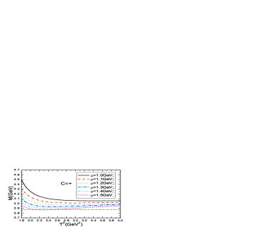
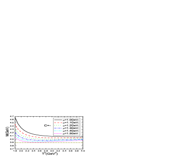
Figure 2: The masses with variations of the Borel parameters $T^{2}$ and energy scales $\mu$, where the horizontal lines denote the experimental values.

In Fig.2, the masses are plotted with variations of the Borel parameters $T^{2}$ and energy scales $\mu$ for the threshold parameter $\sqrt{s_{0}}=4.4\,\rm{GeV}$. From the figure, we can see that the masses decrease monotonously with increase of the energy scales. The energy scale $\mu=1.5\,\rm{GeV}$ is the lowest energy scale to reproduce the experimental data.

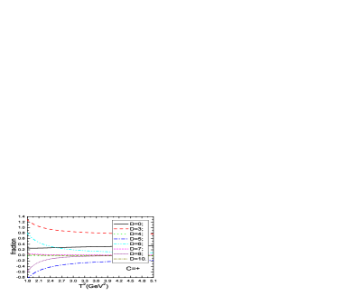
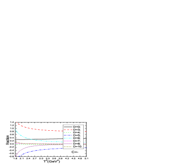
Figure 3: The contributions of different terms in the operator product expansion with variations of the Borel parameters $T^{2}$, where the $D$ denotes the dimensions of the vacuum condensates.

In Fig.3, the contributions of different terms in the operator product expansion are plotted with variations of the Borel parameters $T^{2}$ for the threshold parameter $\sqrt{s_{0}}=4.4\,\rm{GeV}$ and energy scale $\mu=1.5\,\rm{GeV}$. From the figure, we can see that the contributions change quickly with variations of the Borel parameters at the region $T^{2}<2.1\,\rm{GeV}^{2}$, which does not warrant platforms for the masses. At the value $T^{2}=2.2\,\rm{GeV}^{2}$, the $D_{0}$, $D_{3}$, $D_{4}$, $D_{5}$, $D_{6}$, $D_{7}$, $D_{8}$, $D_{10}$ are $0.266$, $1.000$, $-0.017$, $-0.495$, $0.406$, $0.032$, $-0.194$, $0.006$ respectively for the $C=+$ tetraquark state; $0.294$, $1.106$,$-0.013$, $-0.617$, $0.450$, $0.028$, $-0.279$, $0.036$ respectively for the $C=-$ tetraquark state, where the $D_{i}$ with $i=0,\,3,\,4,\,5,\,6,\,7,\,8,\,10$ denote the contributions of the vacuum condensates of dimensions $D=i$, and the total contributions are normalized to be $1$. Although the contributions of the condensates do not decrease monotonously with increase of dimensions, the $D_{4}$, $D_{7}$, $D_{10}$ play a less important role, $D_{3}\gg|D_{5}|>D_{6}\gg D_{8}$, the $D_{6}$, $D_{8}$, $D_{10}$ decrease monotonously and quickly with increase of the Borel parameters. The convergence of the operator product expansion does not mean that the perturbative terms make dominant contributions, as the continuum hadronic spectral densities are approximated by $\rho_{QCD}(s)\Theta(s-s_{0})$ in the QCD sum rules for the tetraquark states, where the $\rho_{QCD}(s)$ denotes the full QCD spectral densities; the contributions of the quark condensate $\langle\bar{q}q\rangle$ (of dimension-3) can be very large. In this article, the value $T^{2}\geq 2.2\,\rm{GeV}^{2}$ is taken tentatively, and the convergent behavior in the operator product expansion is very good.

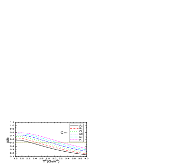
Figure 4: The pole contributions with variations of the Borel parameters $T^{2}$ and threshold parameters $s_{0}$, where the $A$, $B$, $C$, $D$, $E$, $F$ denote the threshold parameters $\sqrt{s_{0}}=4.1$, $4.2$, $4.3$, $4.4$, $4.5$, $4.6\,\rm{GeV}$, respectively.

In Fig.4, the contributions of the pole terms are plotted with variations of the threshold parameters $s_{0}$ and Borel parameters $T^{2}$ at the energy scale $\mu=1.5\,\rm{GeV}$. From the figure, we can see that the values $\sqrt{s_{0}}\leq 4.2\,\rm{GeV}$ are too small to satisfy the pole dominance condition and result in reasonable Borel platforms. If we take the values $\sqrt{s_{0}}=(4.3-4.5)\,\rm{GeV}$ and $T^{2}=(2.2-2.8)\,\rm{GeV}^{2}$, the pole contributions are about $(49-75)\%$ and $(48-73)\%$ for the $C=+$ and $-$ tetraquark states respectively. The pole dominance condition is well satisfied.

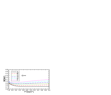
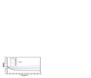
Figure 5: The masses with variations of the Borel parameters $T^{2}$ and threshold parameters $s_{0}$, where the $A$, $B$, $C$, $D$, $E$, $F$ denote the threshold parameters $\sqrt{s_{0}}=4.1$, $4.2$, $4.3$, $4.4$, $4.5$, $4.6\,\rm{GeV}$, respectively, and the horizontal lines denote the experimental values.

In Fig.5, the predicted masses are plotted with variations of the threshold parameters $s_{0}$ and Borel parameters $T^{2}$ at the energy scale $\mu=1.5\,\rm{GeV}$. From the figure, we can see that the value $\sqrt{s_{0}}=4.4\,\rm{GeV}$ is the optimal value to reproduce the experimental data. In this article, the parameters $\sqrt{s_{0}}=(4.3-4.5)\,\rm{GeV}$, $T^{2}=(2.2-2.8)\,\rm{GeV}^{2}$ and $\mu=1.5\,\rm{GeV}$ are taken.

Taking into account all uncertainties of the input parameters, finally we obtain the values of the masses and pole residues of the $X(3872)$ and $Z_{c}(3900)$ (or $Z_{c}(3885)$), which are shown explicitly in Figs.6-7,

$$M_{X} = 3.87^{+0.09}_{-0.09}\,\rm{GeV}\,,$$

$$M_{Z} = 3.91^{+0.11}_{-0.09}\,\rm{GeV}\,,$$

$$\lambda_{X} = 2.15^{+0.36}_{-0.27}\times 10^{-2}\,\rm{GeV}^{5}\,,$$

$$\lambda_{Z} = 2.20^{+0.36}_{-0.29}\times 10^{-2}\,\rm{GeV}^{5}\,.$$ (28)

The uncertainties of the masses are very small, about $2.5\%$, as the uncertainties induced by the input parameters are canceled out to some extents between the numerators and denominators, see Eq.(24); on the other hand, the uncertainties of the pole residues are much large, about $15\%$, as no cancelation occurs among the induced uncertainties, see Eq.(19). The prediction $M_{X}=3.87^{+0.09}_{-0.09}\,\rm{GeV}$ is consistent with the experimental data $M_{X(3872)}=(3871.68\pm 0.17)\,\rm{MeV}$ [27], and the prediction $M_{Z}=3.91^{+0.11}_{-0.09}\,\rm{GeV}$ is also consistent with the experimental data $M_{Z_{c}(3900)}=(3899.0\pm 3.6\pm 4.9)\,\rm{MeV}$ [17] and $M_{Z_{c}(3885)}=(3883.9\pm 1.5\pm 4.2)\,\rm{MeV}$ [25] within uncertainties. The present predictions favor identifying the $X(3872)$ and $Z_{c}(3900)$ (or $Z_{c}(3885)$) as the $J^{PC}=1^{++}$ and $1^{+-}$ diquark-antidiquark type tetraquark states, respectively. There is a small energy gap less than $40\,\rm{MeV}$ between the central values of the masses of the $C=+$ and $C=-$ axial-vector tetraquark states, which is consistent with the value $10\,\rm{MeV}$ from the constituent diquark model [9, 20]. The central values originate from the central values of all the input parameters. We should bear in mind that the masses alone cannot qualify the assignments ambiguously, furthermore, the $M_{X}$ and $M_{Z}$ degenerate according to the uncertainties.

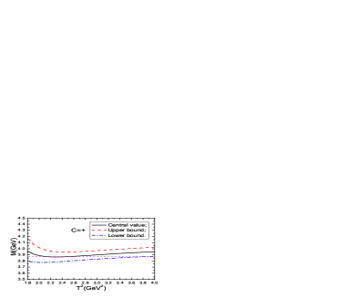
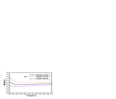
Figure 6: The masses with variations of the Borel parameters $T^{2}$, where the horizontal lines denote the experimental values.

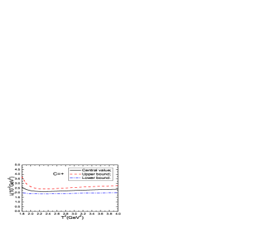
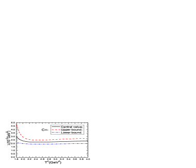
Figure 7: The pole residues with variations of the Borel parameters $T^{2}$.

4 Conclusion

In this article, we distinguish the charge conjunctions of the interpolating currents, calculate the contributions of the vacuum condensates up to dimension-10 in a consistent way in the operator product expansion and discard the perturbative corrections, and take into account the higher dimensional vacuum condensates neglected in previous works, as they play an important role in determining the Borel windows. Then we study the $J^{PC}=1^{+\pm}$ diquark-antidiquark type hidden charmed tetraquark states with the QCD sum rules, explore the energy scale dependence in details for the first time, and make reasonable predictions of the masses $M_{X}=3.87^{+0.09}_{-0.09}\,\rm{GeV}$, $M_{Z}=3.91^{+0.11}_{-0.09}\,\rm{GeV}$ and pole residues $f_{X}=2.15^{+0.36}_{-0.27}\times 10^{-2}\,\rm{GeV}^{5}$, $f_{Z}=2.20^{+0.36}_{-0.29}\times 10^{-2}\,\rm{GeV}^{5}$. In calculations, we observe that the tetraquark masses decrease monotonously with increase of the energy scales, $\mu=1.5\,\rm{GeV}$ is the lowest energy scale to reproduce the experimental data. The energy scale $\mu=1.5\,\rm{GeV}$ can also lead to reasonable masses for the charmed mesons $D$ and $J/\psi$, and serves as an acceptable energy scale for the charmed mesons in the QCD sum rules. The predictions support identifying the $X(3872)$ and $Z_{c}(3900)$ (or $Z_{c}(3885)$) as the $1^{++}$ and $1^{+-}$ diquark-antidiquark type tetraquark states, respectively. The pole residues can be taken as basic input parameters to study relevant processes of the $X(3872)$ and $Z_{c}(3900)$ (or $Z_{c}(3885)$) with the three-point QCD sum rules.

References

[1] F. E. Close and N. A. Tornqvist, J. Phys. G28 (2002) R249;
R. L. Jaffe, Phys. Rept. 409 (2005) 1;
C. Amsler and N. A. Tornqvist, Phys. Rept. 389 (2004) 61;
E. Klempt and A. Zaitsev, Phys. Rept. 454 (2007) 1.
[2] T. V. Brito, F. S. Navarra, M. Nielsen and M. E. Bracco, Phys. Lett. B608 (2005) 69;
Z. G. Wang and W. M. Yang, Eur. Phys. J. C42 (2005) 89;
Z. G. Wang, W. M. Yang and S. L. Wan, J. Phys. G31 (2005) 971;
H. J. Lee and N. I. Kochelev, Phys. Lett. B642 (2006) 358;
A. Zhang, T. Huang and T. G. Steele, Phys. Rev. D76 (2007) 036004;
A. Zhang, T. Huang and T. Steele, Prog. Theor. Phys. Suppl. 168 (2007) 198;
H. X. Chen, A. Hosaka and S. L. Zhu, Phys. Rev. D76 (2007) 094025;
Z. G. Wang, Int. J. Theor. Phys. 51 (2012) 507.
[3] M. A. Shifman, A. I. Vainshtein and V. I. Zakharov, Nucl. Phys. B147 (1979) 385.
[4] L. J. Reinders, H. Rubinstein and S. Yazaki, Phys. Rept. 127 (1985) 1.
[5] Z. G. Wang, Nucl. Phys. A791 (2007) 106.
[6] S. K. Choi et al, Phys. Rev. Lett. 91 (2003) 262001.
[7] K. Abe et al, hep-ex/0505037; B. Aubert et al, Phys. Rev. D74 (2006) 071101;
B. Aubert et al, Phys. Rev. Lett. 102 (2009) 132001.
[8] K. Abe et al, hep-ex/0505038; A. Abulencia et al, Phys. Rev. Lett. 98 (2007) 132002;
S. K. Choi et al, Phys. Rev. D84 (2011) 052004; R Aaij et al, Phys. Rev. Lett. 110 (2013) 222001.
[9] L. Maiani, F. Piccinini, A. D. Polosa and V. Riquer, Phys. Rev. D71 (2005) 014028.
[10] E. S. Swanson, Phys. Rept. 429 (2006) 243;
S. Godfrey and S. L. Olsen, Ann. Rev. Nucl. Part. Sci. 58 (2008) 51;
M. B. Voloshin, Prog. Part. Nucl. Phys. 61 (2008) 455;
N. Drenska, R. Faccini, F. Piccinini, A. Polosa, F. Renga and C. Sabelli, Riv. Nuovo Cim. 033 (2010) 633.
[11] R. D. Matheus, S. Narison, M. Nielsen and J. M. Richard, Phys. Rev. D75 (2007) 014005.
[12] F. S. Navarra, M. Nielsen and S. H. Lee, Phys. Lett. B649 (2007) 166;
S. H. Lee, A. Mihara, F. S. Navarra and M. Nielsen, Phys. Lett. B661 (2008) 28;
R. M. Albuquerque and M. Nielsen, Nucl. Phys. A815 (2009) 53;
M. E. Bracco, S. H. Lee, M. Nielsen and R. Rodrigues da Silva, Phys. Lett. B671 (2009) 240;
W. Chen and S. L. Zhu , Phys. Rev. D81 (2010) 105018;
J. R. Zhang and M. Q. Huang, JHEP 1011 (2010) 057;
J. R. Zhang and M. Q. Huang, Phys. Rev. D83 (2011) 036005;
S. Narison, F. S. Navarra and M. Nielsen, Phys. Rev. D83 (2011) 016004;
W. Chen and S. L. Zhu, Phys. Rev. D83 (2011) 034010;
C. Y. Cui, Y. L. Liu, G. B. Zhang and M. Q. Huang, Commun. Theor. Phys. 57 (2012) 1033;
J. M. Dias, R. M. Albuquerque, M. Nielsen and C. M. Zanetti, Phys. Rev. D86 (2012) 116012;
M. L. Du, W. Chen, X. L. Chen and S. L. Zhu, Phys. Rev. D87 (2013) 014003;
C. F. Qiao and L. Tang, arXiv:1308.3439.
[13] Z. G. Wang, Eur. Phys. J. C59 (2009) 675;
Z. G. Wang, Eur. Phys. J. C62 (2009) 375;
Z. G. Wang, Phys. Rev. D79 (2009) 094027;
Z. G. Wang, J. Phys. G36 (2009) 085002;
Z. G. Wang, Eur. Phys. J. C67 (2010) 411;
Z. G. Wang, Y. M. Xu and H. J. Wang, Commun. Theor. Phys. 55 (2011) 1049.
[14] Z. G. Wang, Eur. Phys. J. C70 (2010) 139.
[15] C. F. Qiao and L. Tang, arXiv:1307.6654.
[16] N. Brambilla et al Eur. Phys. J. C71 (2011) 1534.
[17] M. Ablikim et al, Phys. Rev. Lett. 110 (2013) 252001.
[18] Z. Q. Liu et al, Phys. Rev. Lett. 110 (2013) 252002.
[19] T. Xiao, S. Dobbs, A. Tomaradze and K. K. Seth, Phys. Lett. B727 (2013) 366.
[20] R. Faccini, L. Maiani, F. Piccinini, A. Pilloni, A. D. Polosa and V. Riquer, Phys. Rev. D87 (2013) 111102(R).
[21] F. K. Guo, C. Hidalgo-Duque, J. Nieves and M. P. Valderrama, Phys. Rev. D88 (2013) 054007;
C. Y. Cui, Y. L. Liu, W. B. Chen and M. Q. Huang, arXiv:1304.1850;
J. R. Zhang, Phys. Rev. D87 (2013) 116004;
Y. Dong, A. Faessler, T. Gutsche and V. E. Lyubovitskij, Phys. Rev. D88 (2013) 014030;
H. W. Ke, Z. T. Wei and X. Q. Li, Eur. Phys. J. C73 (2013) 2561;
S. Prelovsek and L. Leskovec, Phys. Lett. B727 (2013) 172.
[22] M. Karliner and S. Nussinov, JHEP 1307 (2013) 153;
N. Mahajan, arXiv:1304.1301;
J. M. Dias, F. S. Navarra, M. Nielsen and C. M. Zanetti, Phys. Rev. D88 (2013) 016004;
E. Braaten, arXiv:1305.6905.
[23] M. B. Voloshin, Phys. Rev. D87 (2013) 091501.
[24] D. Y. Chen, X. Liu and T. Matsuki, Phys. Rev. Lett. 110 (2013) 232001;
Q. Wang, C. Hanhart and Q. Zhao, Phys. Rev. Lett. 111 (2013) 132003;
Q. Wang, C. Hanhart and Q. Zhao, Phys. Lett. B725 (2013) 106;
X. H. Liu and G. Li, Phys. Rev. D88 (2013) 014013.
[25] M. Ablikim et al, Phys. Rev. Lett. 112 (2014) 022001.
[26] Z. G. Wang, Eur. Phys. J. C63 (2009) 115;
Z. G. Wang, Z. C. Liu and X. H. Zhang, Eur. Phys. J. C64 (2009) 373;
Z. G. Wang, Phys. Lett. B690 (2010) 403;
Z. G. Wang and X. H. Zhang, Commun. Theor. Phys. 54 (2010) 323.
[27] J. Beringer et al, Phys. Rev. D86 (2012) 010001.
[28] W. Hubschmid and S. Mallik, Nucl. Phys. B207 (1982) 29;
V. A. Novikov, M. A. Shifman, A. I. Vainshtein and V. I. Zakharov, Fortsch. Phys. 32 (1984) 585.
[29] B. L. Ioffe, Prog. Part. Nucl. Phys. 56 (2006) 232.
[30] P. Colangelo and A. Khodjamirian, hep-ph/0010175.
[31] Z. G. Wang, JHEP 1310 (2013) 208.
[32] Z. G. Wang, Phys. Rev. D83 (2011) 014009; B. Chen, L. Yuan and A. Zhang, Phys. Rev. D83 (2011) 114025;
A. M. Badalian and B. L. G. Bakker, Phys. Rev. D84 (2011) 034006;
P. Colangelo, F. De Fazio, F. Giannuzzi and S. Nicotri, Phys. Rev. D86 (2012) 054024;
Z. G. Wang, Phys. Rev. D88 (2013) 114003.