$Z_{c}(3900)$: Confronting theory and lattice simulations

Abstract

We consider a recent $T$-matrix analysis by Albaladejo et al., [Phys. Lett. B 755, 337 (2016)] which accounts for the $J/\psi\pi$ and $D^{\ast}\bar{D}$ coupled–channels dynamics, and that successfully describes the experimental information concerning the recently discovered $Z_{c}(3900)^{\pm}$. Within such scheme, the data can be similarly well described in two different scenarios, where the $Z_{c}(3900)$ is either a resonance or a virtual state. To shed light into the nature of this state, we apply this formalism in a finite box with the aim of comparing with recent Lattice QCD (LQCD) simulations. We see that the energy levels obtained for both scenarios agree well with those obtained in the single-volume LQCD simulation reported in Prelovsek et al. [Phys. Rev. D 91, 014504 (2015)], making thus difficult to disentangle between both possibilities. We also study the volume dependence of the energy levels obtained with our formalism, and suggest that LQCD simulations performed at several volumes could help in discerning the actual nature of the intriguing $Z_{c}(3900)$ state.

I Introduction

Since the discovery of the $X(3872)$ in 2003 Choi:2003ue , the charmonium and charmonium-like spectrum are being continuously enlarged with new so-called $XYZ$ states Olsen:2014qna ; Chen:2016qju ; Hosaka:2016pey , many of which do not fit properly in the conventional quark models Godfrey:1985xj . The relevance of meson-meson channels can be grasped from the fact that all the charmonium states predicted below the lowest hidden-charm threshold ($D\bar{D}$) have been experimentally confirmed, but above this energy most of the observed states cannot be unambiguously identified with any of the predicted charmonium $c\bar{c}$ states.

Amongst the $XYZ$ states, the $Z_{c}(3900)^{\pm}$ was simultaneously discovered by the BESIII and Belle collaborations Ablikim:2013mio ; Liu:2013dau in the $e^{+}e^{-}\to Y(4260)\to J/\psi\pi^{+}\pi^{-}$ reaction, where a clear peak very close to the $D^{\ast}\bar{D}$ threshold, around $3.9\ \text{GeV}$, is seen in the $J/\psi\pi$ spectrum. Later on, an analysis Xiao:2013iha based on CLEO-c data for a different reaction, $e^{+}e^{-}\to\psi(4160)\to J/\psi\pi^{+}\pi^{-}$, confirmed the presence of this resonant structure as well, although with a somewhat lower mass. The BESIII collaboration Ablikim:2013xfr ; Ablikim:2015swa has also reported a resonant-like structure in the $\bar{D}^{\ast}D$ spectrum for the reaction $e^{+}e^{-}\to\bar{D}^{*}D\pi$ at different $e^{+}e^{-}$ center-of-mass (c.m.) energies [including the production of $Y(4260)$]. This structure, with quantum numbers favored to be $J^{P}=1^{+}$, has been cautiously called $Z_{c}(3885)^{\pm}$, because its fitted mass and width showed some differences with those attributed to the $Z_{c}(3900)^{\pm}$. Whether both set of observations correspond to the same state needs to be confirmed, though there is a certain consensus that this is indeed the case, and the peaks reported as the $Z_{c}(3885)^{\pm}$ and $Z_{c}(3900)^{\pm}$ are originated by the same state seen in different channels. Moreover, evidence for its neutral partner, $Z_{c}(3900)^{0}$, has also been reported Xiao:2013iha ; Ablikim:2015tbp .

The nature of the $Z_{c}\left(3900\right)^{\pm}$ is intriguing. On one hand, it couples to $D^{\ast}\bar{D}$ and $J/\psi\pi$, and therefore one assumes it should contain a constituent $c\bar{c}$ quark–anti-quark pair. On the other hand, it is charged and hence it must also have another constituent quark–anti-quark pair, namely $u\bar{d}$ (for $Z_{c}^{+}$). Its minimal structure would be then $c\bar{c}u\bar{d}$, which automatically qualifies it as a non-$q\bar{q}$ (exotic) meson. Being a candidate for an exotic hidden charm state, it has triggered much theoretical interest. An early discussion of possible structures for the $Z_{c}\left(3900\right)^{\pm}$ was given in Ref. Voloshin:2013dpa . The suggested interpretations cover a wide range: a $\bar{D}^{\ast}D$ molecule Wang:2013cya ; Guo:2013sya ; Wilbring:2013cha ; Dong:2013iqa ; Zhang:2013aoa ; Ke:2013gia ; Aceti:2014uea ; He:2015mja , a tetraquark Braaten:2013boa ; Wang:2013vex ; Dias:2013xfa ; Deng:2014gqa ; Qiao:2013raa ; Esposito:2014rxa ; Maiani:2014aja , an object originated from an attractive $\bar{D}^{\ast}D^{\ast}$ interaction Zhou:2015jta , a simple kinematical effect Chen:2013coa ; Swanson:2014tra , a cusp enhancement due to a triangle singularity Szczepaniak:2015eza , or a radially excited axial meson Coito:2016ads . In Ref. Guo:2014iya , it was argued that this structure cannot be a kinematical effect and that it must necessarily be originated from a nearby pole. Consequences from some of these models have been discussed in Ref. Cleven:2015era . The non-compatibility (partial or total) of the properties of the $Z_{c}$ deduced in different approaches clearly hints why the actual nature of this state has attracted so much attention.

In Ref. Albaladejo:2015lob , theoretical basis of the present manuscript, a $J/\psi\pi$–$D^{\ast}\bar{D}$ coupled-channels scheme was proposed to describe the observed peaks associated to the $Z_{c}(3900)$, which is assumed to have $I(J^{PC})=1(1^{+-})$ quantum numbers. Within this coupled channel scheme, it was possible to successfully describe simultaneously the BESIII $J\psi\pi$ Ablikim:2013mio and $D^{\ast}\bar{D}$ Ablikim:2015swa invariant mass spectra, in which the $Z_{c}(3900)^{\pm}$ structure has been seen. Interestingly, two different fits with similar quality were able to reproduce the data. In each of them, the origin of the $Z_{c}(3900)^{\pm}$ was different. In the first scenario, it corresponded to a resonance originated from a pole above the $D^{\ast}\bar{D}$ threshold, whereas in the second one the structure was produced by a virtual pole below the threshold (see Ref. Albaladejo:2015lob for more details).

Hadron interactions are governed by the non-perturbative regime of QCD and, for this reason, Lattice QCD (LQCD) is an essential theoretical tool in hadron physics. In particular, one of the aims of LQCD is to obtain the hadron spectrum from quarks and gluons and their interactions (see e.g. Ref.Fodor:2012gf for a review focused on the light sector, and Refs. Dudek:2007wv ; Bali:2011rd ; Liu:2012ze ; Lang:2015sba for results concerning the charmonium sector). For such a purpose the Lüscher method Luscher:1986pf ; Luscher:1990ux is widely used. It relates the discrete energy levels of a two-hadron system in a finite box with the phase shifts and/or binding energies of that system in an infinite volume. Appropriate generalizations relevant for our work can be found in Refs. Liu:2005kr ; Lage:2009zv ; Bernard:2010fp ; Doring:2011vk .

LQCD simulations devoted to find the $Z_{c}(3900)$ state are still scarce Prelovsek:2013xba ; Prelovsek:2014swa ; Chen:2014afa ; Liu:2014mfy ; Lee:2014uta ; Ikeda:2016zwx . Exploratory theoretical studies for hidden charm molecules have been performed in Refs. Albaladejo:2013aka ; Garzon:2013uwa , while actual LQCD simulations Prelovsek:2013xba ; Prelovsek:2014swa ; Chen:2014afa ; Liu:2014mfy ; Lee:2014uta find energy levels showing a weak interaction in the $Z_{c}(3900)^{\pm}$ quantum-numbers sector (either attractive or repulsive), and no evidence is found for its existence. The work of Ref. Ikeda:2016zwx employs LQCD to obtain a coupled-channel $S$-matrix, which shows an interaction dominated by off-diagonal terms, and, according to Ref. Ikeda:2016zwx , this does not support a usual resonance picture for the $Z_{c}(3900)$. This $S$-matrix contains a pole located well below threshold in an unphysical Riemann sheet, i.e., a virtual pole. It is worth to note that this possibility could be in agreement with the second scenario advocated in Ref. Albaladejo:2015lob , and mentioned above.

Our objective in the present manuscript is to implement the coupled channel $T$-matrix fitted to data in Ref. Albaladejo:2015lob in a finite volume and study its spectrum. Thus, we will be able to compare the energy levels obtained with this finite volume $T$-matrix with those obtained in LQCD simulations, in particular those reported in Ref. Prelovsek:2014swa . This work is organized as follows. The formalism is presented in Sec. II, while the $T$-matrix of Ref. Albaladejo:2015lob is briefly discussed in Subsec. II.1, and its extension for a finite volume is outlined in Subsec. II.2. Results are presented and discussed in Sec. III, and the conclusions of this work, together with a brief summary are given in Sec. IV.

II Formalism

Table 1: Values of the parameters employed in Eq. (8), taken from Ref. Albaladejo:2015lob , together with the $Z_{c}$ pole positions found in that work. The errors account for statistical (first) and systematic (second) uncertainties (see Ref. Albaladejo:2015lob for details).

$\displaystyle\frac{a}{b}$ $\Lambda_{2}\ (\text{GeV})$	$C_{1Z}\ (\text{fm}^{2})$	$b\ (\text{fm}^{3})$	$\widetilde{C}\ (\text{fm}^{2})$	$M_{Z_{c}}\ (\text{MeV})$	$\Gamma_{Z_{c}}/2\ (\text{MeV})$
$1.0$	$-0.19\pm 0.08\pm 0.01$	$-2.0\pm 0.7\pm 0.4$	$0.39\pm 0.10\pm 0.02$	$3894\pm 6\pm 1$	$30\pm 12\pm 6$
$0.5$	$\hphantom{+}0.01\pm 0.21\pm 0.03$	$-7.0\pm 0.4\pm 1.4$	$0.64\pm 0.16\pm 0.02$	$3886\pm 4\pm 1$	$22\pm\hphantom{1}6\pm 4$
$1.0$	$-0.27\pm 0.08\pm 0.07$	$0$ (fixed)	$0.34\pm 0.14\pm 0.01$	$3831\pm 26^{+\hphantom{1}7}_{-28}$	virtual state
$0.5$	$-0.27\pm 0.16\pm 0.13$	$0$ (fixed)	$0.54\pm 0.16\pm 0.02$	$3844\pm 19^{+12}_{-21}$	virtual state

II.1 Infinite volume

We first briefly review the model of Ref. Albaladejo:2015lob (where the reader is referred for more details) that we are going to employ here. There, the $Y(4260)$ decays to $D\bar{D}^{\ast}\pi$ and $J/\psi\pi\pi$ are studied with a model shown diagrammatically in Fig. 1 of that reference. Final state interactions among the outgoing $D\bar{D}^{\ast}$ and $J/\psi\pi$ produce the peaks observed by the BESIII collaboration, which are associated to the $Z_{c}(3900)$ state. The two channels involved in the $1(1^{+})$ $T$-matrix are denoted as $1\equiv J/\psi\pi$ and $2\equiv D\bar{D}^{\ast}$. Solving the on-shell version of the factorized Bethe-Salpeter equation (BSE) allows to write:

$$T^{-1}(E)=V^{-1}(E)-G(E),$$ (1)

where $E$ is the c.m. energy of the system. The symmetric $V$ matrix is the potential kernel, whose matrix elements have the following form:

$$V_{ij}=4\sqrt{m_{i,1}m_{i,2}m_{j,1}m_{j,2}}\ C_{ij}\ e^{-k^{2}_{i}/\Lambda^{2}_{i}}e^{-k^{2}_{j}\,/\Lambda^{2}_{j}}.$$ (2)

with $m_{i,1}$ and $m_{i,2}$ the masses of the particles of the $i$th channel and $k_{i}^{2}$, the relative three-momenta squared in the c.m. frame, implicitly defined through:

$$E =\omega_{\psi}(k_{1})+\omega_{\pi}(k_{1}),$$ (3)

$$E =\omega_{D^{\ast}\bar{D}}(k_{2})~{},$$ (4)

where:

$$\omega_{\psi}(q) =\sqrt{m_{J/\psi}^{2}+q^{2}}~{},$$ (5)

$$\omega_{\pi}(q) =\sqrt{m_{\pi}^{2}+q^{2}}~{},$$ (6)

$$\omega_{D^{\ast}\bar{D}}(q) =m_{D}+m_{D^{\ast}}+\frac{m_{D}+m_{D^{\ast}}}{2m_{D}m_{D^{\ast}}}q^{2}~{}.$$ (7)

with $q\equiv|\vec{q}\,|$. The Gaussian form factors $e^{-k^{2}_{i}/\Lambda^{2}_{i}}$ are introduced to regularize the BSE, and thus, for each channel, an ultraviolet (UV) cut-off $\Lambda_{i}$ is introduced. In this work, we have used $\Lambda_{1}=1.5\ \text{GeV}$ and two values for $\Lambda_{2}=0.5$ and 1 GeV Nieves:2012tt ; HidalgoDuque:2012pq . The $C_{ij}$ matrix stands for the $S$-wave interaction in the coupled-channels space, and it is given by Albaladejo:2015lob :

$$C =\begin{bmatrix}0&\tilde{C}\\ \tilde{C}&C_{22}\left(E\right)\\ \end{bmatrix}.$$ (8)

In Eq. (8) the $J/\psi\pi\to J/\psi\pi$ interaction is neglected, $C_{11}=0$, the inelastic transition one is approximated by a constant, $\tilde{C}$, while the $D^{\ast}\bar{D}\to D^{\ast}\bar{D}$ potential $C_{22}(E)$ is parametrized as:

$$C_{22}(E)=C_{1Z}+b\left(E-m_{D}-m_{D^{\ast}}\right).$$ (9)

In a momentum expansion, the lowest order contact potential for this elastic transition would be simply a constant, $C_{22}\equiv C_{1Z}$. However, it is easy to prove that two coupled channels with contact potentials cannot generate a resonance above threshold. Thus and for the sake of generality, the model of Ref. Albaladejo:2015lob allows for an energy dependence in Eq. (9), driven by the $b$ parameter. The $G$ matrix in Eq. (1) is diagonal, and its matrix elements are the $J/\psi\pi$ and $D^{\ast}\bar{D}$ loop functions,

$$G_{11}(E) =\int_{\mathbb{R}^{3}}\frac{{\rm d}^{3}q}{\left(2\pi\right)^{3}}\frac{\omega_{\psi}(q)+\omega_{\pi}(q)}{2\omega_{\psi}(q)\omega_{\pi}(q)}\frac{e^{-2\left(q^{2}-k_{1}^{2}\right)/\Lambda_{1}^{2}}}{E^{2}-\left(\omega_{\psi}(q)+\omega_{\pi}(q)\right)^{2}+i\epsilon}~{},$$ (10)

$$G_{22}(E) =\frac{1}{4m_{D}m_{D^{\ast}}}\int_{\mathbb{R}^{3}}\frac{{\rm d}^{3}q}{\left(2\pi\right)^{3}}\frac{e^{-2\left(q^{2}-k_{2}^{2}\right)/\Lambda_{2}^{2}}}{E-\omega_{D\bar{D}^{\ast}}(q)+i\epsilon}~{},$$ (11)

which account for the right-hand cut of the $T$-matrix, that satisfies in this way the optical theorem. The $D^{\ast}\bar{D}$ channel loop function $G_{22}$ is computed in the non-relativistic approximation.

The free parameters in the interaction matrix $C$ ($\tilde{C}$, $C_{1Z}$ and $b$) were fitted in Ref. Albaladejo:2015lob to the experimental $J/\psi\pi^{-}$ and $D^{+}D^{\ast-}$ invariant mass distributions in the $Y(4260)\to J/\psi\pi\pi$ and $Y(4260)\to D\bar{D}^{\ast}\pi$ decays Ablikim:2013mio ; Ablikim:2015swa . The fitted parameters are compiled here in Table 1, where we can see the two different scenarios investigated in Ref. Albaladejo:2015lob . In the first one, $b\neq 0$, the $Z_{c}$ appears as a $D^{\ast}\bar{D}$ resonance, i.e., a pole above the $D^{\ast}\bar{D}$ threshold in a Riemann sheet connected with the physical one above this energy. In the second one, where $b=0$, a pole appeared below the $D\bar{D}^{\ast}$ threshold in an unphysical Riemann sheet, which gives rise to the $Z_{c}(3900)$ structure, peaking exactly at the $D^{\ast}\bar{D}$ threshold in this case Albaladejo:2015lob (see also Ref. Albaladejo:2015dsa ).

II.2 Finite volume

In this subsection, we study the previous coupled channel $T$-matrix in a finite volume. The consequence of putting the interaction in a box of size $L$ with periodic boundary conditions is that the three-momentum is no longer a continuous variable, but a discrete one. For each value of $L$, we have the infinite set of momenta $\vec{q}=\frac{2\pi}{L}\vec{n}$, $\vec{n}\in\mathbb{Z}^{3}$. The integrals in Eqs. (10) and (11) will be replaced by sums over all the possible values of $\vec{q}$:

$$\tilde{G}_{11}(E) =\frac{1}{L^{3}}\sum_{\vec{n}}\frac{\omega_{\psi}(q)+\omega_{\pi}(q)}{2\omega_{\psi}(q)\omega_{\pi}(q)}\frac{e^{-2\left(q^{2}-k_{1}^{2}\right)/\Lambda_{1}^{2}}}{E^{2}-\left(\omega_{\psi}(q)+\omega_{\pi}(q)\right)^{2}}~{},$$ (12)

$$\tilde{G}_{22}(E) =\frac{1}{4\left(m_{D}m_{D^{\ast}}\right)}\frac{1}{L^{3}}\sum_{\vec{n}}\frac{e^{-2\left(q^{2}-k_{2}^{2}\right)/\Lambda_{2}^{2}}}{E-\omega_{D\bar{D}^{\ast}}(q)}~{},$$ (13)

(see Ref. Albaladejo:2013aka for further details). The $T$-matrix in a finite volume is then:

$$\tilde{T}^{-1}(E)=V^{-1}(E)-\tilde{G}(E)~{},$$ (14)

where the $\tilde{G}$ matrix elements are given by Eqs. (12) and (13). The discrete energy levels in the finite box are given by the poles of the $\tilde{T}$-matrix. If the interaction is switched off, $V\to 0$, the free (or non-interacting) energy levels are given by the poles of the $\tilde{G}_{ii}$ functions,

$$E_{J/\psi\pi}^{(\vec{n}\,^{2})} =\omega_{\psi}(q_{L}n)+\omega_{\pi}(q_{L}n)~{},$$ (15)

$$E_{D^{\ast}\bar{D}}^{(\vec{n}\,^{2})} =\omega_{D\bar{D}^{\ast}}(q_{L}n)~{},$$ (16)

where we use the shorthand $q_{L}=2\pi/L$, and $n=\sqrt{\vec{n}\,^{2}}$. The effect of the interaction is to shift these non-interacting energy levels.

Our purpose is to make contact with the results reported in the LQCD simulation of Ref. Prelovsek:2014swa , and hence we will employ the masses and the energy-momentum dispersion relations used in that work. For the $J/\psi\pi$ channel the dispersion relation in Eq. (3) is still appropriate, but for the case of the $D^{\ast}\bar{D}$ channel, in Eqs. (4) and (7), $\omega_{D\bar{D}^{\ast}}(q)$ must be replaced by Prelovsek:2014swa ; Lang:2014yfa :

$$\omega^{\text{lat}}_{D\bar{D}^{\ast}}(q)=m_{D,1}+m_{D^{\ast},1}+\frac{m_{D,2}+m_{D^{\ast},2}}{2m_{D,2}m_{D^{\ast},2}}q^{2}-\frac{m_{D,4}^{3}+m_{D^{\ast},4}^{3}}{8m_{D,4}^{3}m_{D^{\ast},4}^{3}}q^{4}~{}.$$ (17)

This lattice energy of the $D^{\ast}\bar{D}$ pair suffers from discretization errors and it must be used in Eq. (13). The non-interacting energy levels in Eq. (16) should be also modified accordingly. Notice that, because of the factor $e^{-q^{2}/\Lambda^{2}}$, the sum in Eq. (13) is exponentially suppressed in $\vec{n}\,^{2}$. For the range of energies considered in this work, it is sufficient to add terms up to $\vec{n}\,^{2}=6$.

Table 2: Lattice parameters taken from Refs. Prelovsek:2014swa ; Lang:2014yfa , and employed in this work.

Lengths (fm)
	$a$	$0.1239(13)$
	$L=16a$	$1.982(21)$
Masses (lattice units)
	$am_{\pi}$	$0.1673(16)$
	$am_{J/\psi}$	$1.54171(43)$
	$am_{\eta_{c}}$	$1.47392(31)$
	$am_{D,1}$	$0.9801(10)$
	$am_{D,2}$	$1.107(12)$
	$am_{D,4}$	$1.107(27)$
	$am_{D^{\ast},1}$	$1.0629(13)$
	$am_{D^{\ast},2}$	$1.267(21)$
	$am_{D^{\ast},4}$	$1.325(68)$

Finally, the discrete, interacting energy levels reported in Ref. Prelovsek:2014swa are actually the result of applying the following shift:

$$E\to E^{\ast}=E-m^{\text{lat}}_{\text{s.a.}}+m^{\text{exp}}_{\text{s.a.}}~{},$$ (18)

where the spin-average mass $m_{\text{s.a.}}$ is given by $m_{\text{s.a.}}=\frac{1}{4}(m_{\eta_{c}}+3m_{J/\psi})$. For this reason, we will also present our energy levels shifted as in Eq. (18). The parameters involved in our calculations, taken from Refs. Prelovsek:2014swa ; Lang:2014yfa , are collected in Table 2. In particular, one has $m_{\pi}=266\pm 4\ \text{MeV}$ and $L=16\,a=1.98\pm 0.02\ \text{fm}$, being $a$ the lattice spacing.

II.3 Further comments

With all the ingredients presented in Subsec. II.2, we can compare our predictions for the energy levels in a box with those reported in Ref. Prelovsek:2014swa . But before presenting our results we would like to discuss some technical details concerning two differences that could affect the comparison.

First, we would like to note that the LQCD simulation in Ref. Prelovsek:2014swa includes the $J/\psi\pi$ and $D^{\ast}\bar{D}$ channels that are present in our $T$-matrix analysis, but it also includes other channels (like $\eta_{c}\rho$ or $D^{\ast}\bar{D}^{\ast}$). However, according to Ref. Albaladejo:2015lob , it is sufficient to include the $J/\psi\pi$ and $D^{\ast}\bar{D}$ channels to achieve a good reproduction of the experimental information concerning the $Z_{c}(3900)$. For this reason, we expect that, in first approximation, these other channels could be safely neglected in the calculations.

The second point to be noted is that we are ignoring the possible $m_{\pi}$ dependence of the parameters in the potential, Eq. (8). Nonetheless, the LQCD simulation of Ref. Prelovsek:2014swa is performed for a relatively low pion mass, $m_{\pi}=266\pm 4\ \text{MeV}$, and we thus expect the eventual dependence to be mild. Furthermore, we are going to compare several sets of these parameters (presented in Table 1), which somewhat compensates this effect.

III Results and discussion

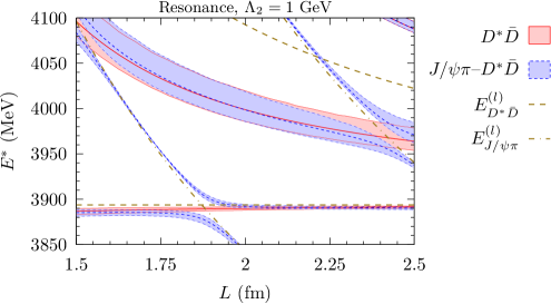
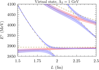
Figure 1: Volume dependence of some energy levels located close to the $D^{\ast}\bar{D}$ threshold, and obtained when the $Z_{c}$ is described as a resonance (left) or as a virtual state (right) in the $L\to\infty$ limit. The blue dashed lines have been obtained from the $J/\psi\pi$–$D^{\ast}\bar{D}$ coupled channel analysis, and the red solid lines show the single elastic channel ($D^{\ast}\bar{D}$) case, in both cases $\Lambda_{2}$ has been fixed to 1 GeV. The error bands are obtained from the uncertainties of the parameters introduced in the theoretical model of Ref. Albaladejo:2015lob (Table 1), adding in quadratures the statistical and systematic errors. The green dashed (dotted-dashed) lines are the free $D^{\ast}\bar{D}$ ($J/\psi\pi$) energy levels $E^{(l\,)}_{D^{\ast}\bar{D}}$ ($E^{(l\,)}_{J/\psi\pi}$).

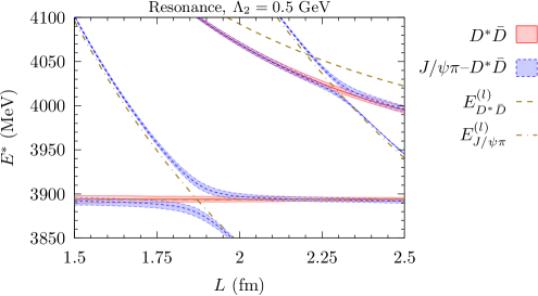
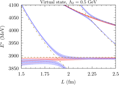
Figure 2: Same as in Fig. 1, but for the case $\Lambda_{2}=0.5\ \text{GeV}$.

In Fig. 1, we show the $L$ dependence of some energy levels close to the $D^{\ast}\bar{D}$ threshold. They have been computed from the poles of the finite volume $\tilde{T}$-matrix, Eq. (14), by using the parameters of Table 1 for $\Lambda_{2}=1\ \text{GeV}$, and the lattice setup given in Table 2. The levels obtained in the $Z_{c}(3900)^{\pm}$ resonance (virtual) scenario, calculated using the entries of the first (third) row of Table 1, are displayed in the left (right) panel. The blue dashed lines stand for the $J/\psi\pi$–$D^{\ast}\bar{D}$ coupled-channel-analysis results, and the red solid lines show the energy levels obtained when the inelastic $J/\psi\pi$–$D^{\ast}\bar{D}$ transition is neglected ($\tilde{C}=0$). This latter case corresponds to consider a single, elastic channel ($D^{\ast}\bar{D}$). The error bands account for the uncertainties on the energy levels inherited from the errors in the parameters of Ref. Albaladejo:2015lob , quoted in Table 1 (statistical and systematical errors are added in quadrature for the calculations). The green dashed (dotted-dashed) lines stand for the non-interacting $D^{\ast}\bar{D}$ ($J/\psi\pi$) energy levels. In Fig. 2, the same results are shown but for the case $\Lambda_{2}=0.5\ \text{GeV}$. The qualitative $L$ behavior of both Figs. 1 and 2 is similar, so we discuss first Fig. 1 and, later on, the specific differences between them will be outlined.

For both resonant and virtual scenarios, there is always an energy level very close to a free energy of the $J/\psi\pi$ state, $E^{(l\,)}_{J/\psi\pi}$, which reveals that the interaction driven by this meson pair is weak. Furthermore, the energy levels for the coupled–channel $\tilde{T}$-matrix basically follow those obtained within the elastic $D^{\ast}\bar{D}$ approximation, except in the neighborhood of the $J/\psi\pi$ free energies. This also corroborates that the role of the $J/\psi\pi$ is not essential.

Let us pay attention to the levels placed in the vicinity of the $D^{\ast}\bar{D}$ threshold. For simplicity, we first look at the single elastic channel case. There appears always a state just below threshold, as it should occur since we are putting an attractive interaction in a finite box. As the size of the box increases, and since there is no bound state in the infinite volume limit (physical case), this level approaches to threshold. When the $J/\psi\pi$ channel is switched on, the $L-$behaviour of this level will be modified, specially when it is close to a discrete $J/\psi\pi$ free energy. Note that the slopes of the $J/\psi\pi$ free levels, in the range of energies considered here, are larger (in absolute value) than those of the $D\bar{D}^{\ast}$ ones, because the threshold of the $J/\psi\pi$ channel is far from the region studied.

From the above discussion, one realizes that the next coupled channel energy level, located between the two $D^{\ast}\bar{D}$ free ones ($E^{\,(0)}_{D^{\ast}\bar{D}}$ and $E^{\,(1)}_{D^{\ast}\bar{D}}$), could be more convenient to extract details of the $Z_{c}(3900)^{\pm}$ dynamics. Indeed, in the resonance scenario, this second energy level is very shifted downwards with respect to $E^{\,(1)}_{D^{\ast}\bar{D}}$, since it is attracted towards the $Z_{c}$ resonance energy. In this context, it should be noted that the presence of $Z_{c}(3900)^{\pm}$ does not induce the appearance of an additional energy level, but a sizeable shift of the energy levels with respect to the non-interacting ones. Therefore, even if no extra energy level appears, it would not be possible to completely discard the existence of a physical state (resonance). The energy shift, however, can be quite large and, only in this sense, one might speak of the appearance of an additional energy level. The correction of the second energy level in the virtual state scenario is much less pronounced. We should note here that the elastic phase shift computed with the $T$-matrix in Ref. Albaladejo:2015lob does not follow the pattern of a standard Breit-Wigner distribution associated to a narrow resonance. Indeed, the phase shift does not change quickly from $0$ to $\pi$ in the vicinity of the $Z_{c}(3900)$ mass, and actually it does not even reach $\pi/2$. This is mostly due to a sizeable background in the amplitude.

We now compare the cases $\Lambda_{2}=1\ \text{GeV}$ (Fig. 1) and $\Lambda_{2}=0.5\ \text{GeV}$ (Fig. 2). For $\Lambda_{2}=0.5\ \text{GeV}$, the relevant (second) energy level is more shifted with respect to $E^{(1)}_{D^{\ast}\bar{D}}$ in the resonance scenario (Fig. 2, left) than in the virtual scenario (Fig. 2, right). This is the same behaviour already discussed for $\Lambda_{2}=1\ \text{GeV}$. However, the shift for the resonance scenario is smaller in the $\Lambda_{2}=0.5\ \text{GeV}$ case (Fig. 2, left) than in the $\Lambda_{2}=1\ \text{GeV}$ one (Fig. 1, left). This is due to the fact that the $Z_{c}(3900)^{\pm}$ is closer to the threshold and the coupling to $D^{\ast}\bar{D}$ is smaller for the $\Lambda_{2}=0.5\ \text{GeV}$ case. Another important difference between the $\Lambda_{2}=1\ \text{GeV}$ and $\Lambda_{2}=0.5\ \text{GeV}$ results is that the error band of the relevant energy level is smaller when the lighter cutoff is used. This is due to the different relative errors in both cases, and the fact that for $\Lambda_{2}=0.5\ \text{GeV}$, the relevant level is closer to the $E^{(1)}_{D^{\ast}\bar{D}}$ free energy than in the $\Lambda_{2}=1\ \text{GeV}$ case.

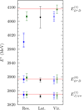
Figure 3: Comparison of the energy levels of Ref. Prelovsek:2014swa , shown with black squares, with our results for $L\simeq 2\ \text{fm}$. Full (empty) circles stand for the energy levels obtained in the resonance (virtual state) scenario for the $Z_{c}(3900)$ state. On the other hand, the energy levels for the $\Lambda_{2}=1\ \text{GeV}$ ($0.5\ \text{GeV}$) case are shown by blue (green) circles. The energy levels calculated in this work are displayed with two types of error bars: the smaller ones have been obtained considering only the errors of the parameters entering in the $T$-matrix (Table 1), whereas the larger ones additionally take into account the errors of the lattice parameters (Table 2).

After having explored the volume dependence of the energy levels predicted with our $\tilde{T}$-matrix and scrutinized its physical meaning, we can now compare our results with those reported in Ref. Prelovsek:2014swa . The energy levels in the latter work are obtained from a single volume simulation, $L=1.98\pm 0.02\ \text{fm}$, and are shown in Fig. 3 with black squares. In the figure, we also show the results obtained in this work for $L=2\ \text{fm}$, for both the resonance (filled circles) and virtual state (empty circles) scenarios for the $Z_{c}(3900)$. Besides, the energy levels calculated with $\Lambda_{2}=1\ \text{GeV}$ and $\Lambda_{2}=0.5\ \text{GeV}$ are represented in blue and green, respectively. We provide two different error bars for our results, considering only the uncertainties of the parameters entering in the $T$-matrix (Table 1), or additionally taking into account the errors of the lattice parameters (Table 2). We clearly see three distinct regions, the lowest energies are very close to the $D\bar{D}^{\ast}$ threshold ($E_{D^{\ast}\bar{D}}^{(0)}$) and to the first $J/\psi\pi$ free energy level ($E^{(1)}_{J/\psi\pi}$). These free energies are shown in Fig. 3 with red solid horizontal lines. As expected, the two lowest lattice levels agree well with our results for both cutoffs and the two $Z_{c}(3900)$ state interpretations examined in this work. The higher energy levels are the relevant ones, and, as already mentioned, our results are significantly shifted to lower energies with respect to $E^{(1)}_{D^{\ast}\bar{D}}$ for the resonant scenario, while this shift is much smaller for the virtual state one. In general, the lattice results are in very good agreement with the virtual state scenario level for both $\Lambda_{2}=0.5\ \text{GeV}$ and $\Lambda_{2}=1\ \text{GeV}$ cases, whereas in the resonance scenario the agreement is also very good for $\Lambda_{2}=0.5\ \text{GeV}$, and it is not so good for $\Lambda_{2}=1\ \text{GeV}$. However, in the latter case, we find $E_{\text{th}}=4000^{+24}_{-13}\ \text{MeV}$, while the lattice energy is $E_{\text{lat}}=4070\pm 30\ \text{MeV}$ Prelovsek:2014swa , and hence this non-compatibility is small, the difference being $E_{\text{lat}}-E_{\text{th}}=70\pm 40\ \text{MeV}$. The comparison of our results with those of Ref. Prelovsek:2014swa support the conclusions given in the latter work: from the energy levels found in that LQCD simulation one cannot deduce the existence of a resonance (a truly physical state, instead of a virtual state), namely $Z_{c}(3900)$. But also from this comparison, putting this conclusion in the other way around, one cannot discard its existence either.

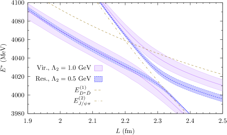
Figure 4: Comparison of the relevant energy level for the $\Lambda_{2}=1\ \text{GeV}$ virtual state (solid purple lines) and the $\Lambda_{2}=0.5\ \text{GeV}$ resonance scenarios (dashed blue lines) around $L\simeq 2\ \text{fm}$. The green dashed and dashed-dotted lines represent $E_{D^{\ast}\bar{D}}^{(1)}$ and $E_{J/\psi\pi}^{(2)}$ non-interacting energies, respectively.

Finally, as can be seen in Fig. 3, a comparison of the relevant energy level obtained in the resonance scenario for $\Lambda_{2}=0.5\ \text{GeV}$ (green filled circle) with that obtained in the virtual scenario for $\Lambda_{2}=1\ \text{GeV}$ (blue empty circle) shows that, within theoretical uncertainties (the smallest error bars), both cases are indistinguishable. This fact can already be seen by comparing the left panel of Fig. 2 and the right panel of Fig. 1 around $L\simeq 2\ \text{fm}$. These energy levels are shown together in Fig. 4. It can be seen that, although these two scenarios cannot be distinguished at $L\simeq 2\ \text{fm}$ (the volume used in Ref. Prelovsek:2014swa ), they lead to appreciably different energies already at $L\simeq 2.5\ \text{fm}$. This means that one cannot elucidate the nature of this intriguing $Z_{c}(3900)$ state with LQCD simulations performed in a single volume. Rather, it would be useful to perform simulations at different values of the box size, to properly study the volume dependence of the energy levels. Of course, as discussed in Ref. Prelovsek:2014swa , this would bring in a technical problem –the appearance of more $J/\psi\pi$ free energy levels in the energy region of interest, as can be seen in Fig. 4 ($E_{J/\psi\pi}^{(2)}$). Notwithstanding these difficulties, our work should stimulate this kind of studies.

IV Summary

With the aim of shedding light into the nature of the $Z_{c}(3900)$ state, we have implemented the $J/\psi\pi$, $D^{\ast}\bar{D}$ coupled channel $T$-matrix of Ref. Albaladejo:2015lob in a finite volume, and we have compared our predictions with the results obtained in the LQCD simulation of Ref. Prelovsek:2014swa . The model of Ref. Albaladejo:2015lob provides a similar good description of the experimental information concerning the $Z_{c}(3900)$ structure in two different scenarios. In the first one, the $Z_{c}(3900)$ structure is due to a resonance originating from the $D^{\ast}\bar{D}$ interaction, while in the second one it is produced by the existence of a virtual state. We have studied the dependence of the energy levels on the size of the finite box for both scenarios. For the volume used in Ref. Prelovsek:2014swa , our results compare well with the energy levels obtained in the LQCD simulation of Ref. Prelovsek:2014swa . However, the agreement is similar in both scenarios (resonant and virtual) and hence it is not possible to privilege one over the other. Therefore and in order to clarify the nature of the $Z_{c}(3900)$ state, we suggest performing further LQCD simulations at different volumes to study the volume dependence of the energy levels.

- [1] S. K. Choi et al. [Belle Collaboration], Phys. Rev. Lett. 91, 262001 (2003).
- [2] S. L. Olsen, Front. Phys. 10, 101401 (2015).
- [3] H. X. Chen, W. Chen, X. Liu and S. L. Zhu, arXiv:1601.02092 [hep-ph].
- [4] A. Hosaka, T. Iijima, K. Miyabayashi, Y. Sakai and S. Yasui, arXiv:1603.09229 [hep-ph].
- [5] S. Godfrey and N. Isgur, Phys. Rev. D 32, 189 (1985).
- [6] M. Ablikim et al. [BESIII Collaboration], Phys. Rev. Lett. 110, 252001 (2013).
- [7] Z. Q. Liu et al. [Belle Collaboration], Phys. Rev. Lett. 110, 252002 (2013).
- [8] T. Xiao, S. Dobbs, A. Tomaradze and K. K. Seth, Phys. Lett. B 727, 366 (2013).
- [9] M. Ablikim et al. [BESIII Collaboration], Phys. Rev. Lett. 112, 022001 (2014).
- [10] M. Ablikim et al. [BESIII Collaboration], Phys. Rev. D 92, 092006 (2015).
- [11] M. Ablikim et al. [BESIII Collaboration], Phys. Rev. Lett. 115, 112003 (2015).
- [12] M. B. Voloshin, Phys. Rev. D 87, 091501 (2013).
- [13] Q. Wang, C. Hanhart and Q. Zhao, Phys. Rev. Lett. 111, 132003 (2013).
- [14] F. K. Guo, C. Hidalgo-Duque, J. Nieves and M. P. Valderrama, Phys. Rev. D 88, 054007 (2013).
- [15] E. Wilbring, H.-W. Hammer and U.-G. Meißner, Phys. Lett. B 726, 326 (2013).
- [16] Y. Dong, A. Faessler, T. Gutsche and V. E. Lyubovitskij, Phys. Rev. D 88, 014030 (2013).
- [17] J. R. Zhang, Phys. Rev. D 87, 116004 (2013).
- [18] H. W. Ke, Z. T. Wei and X. Q. Li, Eur. Phys. J. C 73, 2561 (2013).
- [19] F. Aceti et al., Phys. Rev. D 90, 016003 (2014).
- [20] J. He, Phys. Rev. D 92, 034004 (2015).
- [21] E. Braaten, Phys. Rev. Lett. 111, 162003 (2013).
- [22] J. M. Dias, F. S. Navarra, M. Nielsen and C. M. Zanetti, Phys. Rev. D 88, 016004 (2013).
- [23] L. Maiani, F. Piccinini, A. D. Polosa and V. Riquer, Phys. Rev. D 89, 114010 (2014).
- [24] A. Esposito, A. L. Guerrieri, F. Piccinini, A. Pilloni and A. D. Polosa, Int. J. Mod. Phys. A 30, 1530002 (2015).
- [25] C. F. Qiao and L. Tang, Eur. Phys. J. C 74, 3122 (2014).
- [26] Z. G. Wang and T. Huang, Phys. Rev. D 89, 054019 (2014).
- [27] C. Deng, J. Ping and F. Wang, Phys. Rev. D 90, 054009 (2014).
- [28] Z. Y. Zhou and Z. Xiao, Phys. Rev. D 92, 094024 (2015).
- [29] D. Y. Chen, X. Liu and T. Matsuki, Phys. Rev. D 88, 036008 (2013).
- [30] E. S. Swanson, Phys. Rev. D 91, 034009 (2015).
- [31] A. P. Szczepaniak, Phys. Lett. B 747, 410 (2015).
- [32] S. Coito, arXiv:1602.07821 [hep-ph].
- [33] F. K. Guo, C. Hanhart, Q. Wang and Q. Zhao, Phys. Rev. D 91, 051504, (2015).
- [34] M. Cleven, F. K. Guo, C. Hanhart, Q. Wang and Q. Zhao, Phys. Rev. D 92, 014005 (2015).
- [35] M. Albaladejo, F. K. Guo, C. Hidalgo-Duque and J. Nieves, Phys. Lett. B 755, 337 (2016).
- [36] Z. Fodor and C. Hoelbling, Rev. Mod. Phys. 84, 449 (2012).
- [37] J. J. Dudek, R. G. Edwards, N. Mathur and D. G. Richards, Phys. Rev. D 77, 034501 (2008).
- [38] G. S. Bali, S. Collins and C. Ehmann, Phys. Rev. D 84, 094506 (2011).
- [39] L. Liu et al. [Hadron Spectrum Collaboration], JHEP 1207, 126 (2012).
- [40] C. B. Lang, L. Leskovec, D. Mohler and S. Prelovsek, JHEP 1509, 089 (2015).
- [41] M. Luscher, Commun. Math. Phys. 105, 153 (1986)
- [42] M. Luscher, Nucl. Phys. B 354, 531 (1991).
- [43] C. Liu, X. Feng and S. He, Int. J. Mod. Phys. A 21, 847 (2006).
- [44] M. Lage, U. G. Meissner and A. Rusetsky, Phys. Lett. B 681, 439 (2009).
- [45] V. Bernard, M. Lage, U.-G. Meissner and A. Rusetsky, JHEP 1101, 019 (2011).
- [46] M. Doring, U. G. Meissner, E. Oset and A. Rusetsky, Eur. Phys. J. A 47, 139 (2011).
- [47] S. Prelovsek and L. Leskovec, Phys. Lett. B 727, 172 (2013).
- [48] S. Prelovsek, C. B. Lang, L. Leskovec and D. Mohler, Phys. Rev. D 91, 014504 (2015).
- [49] Y. Chen et al., Phys. Rev. D 89, 094506 (2014).
- [50] L. Liu et al., PoS LATTICE 2014, 117 (2014).
- [51] S. H. Lee et al. [Fermilab Lattice and MILC Collaborations], arXiv:1411.1389 [hep-lat].
- [52] Y. Ikeda et al., arXiv:1602.03465 [hep-lat].
- [53] M. Albaladejo, C. Hidalgo-Duque, J. Nieves and E. Oset, Phys. Rev. D 88, 014510 (2013).
- [54] E. J. Garzon, R. Molina, A. Hosaka and E. Oset, Phys. Rev. D 89, 014504 (2014).
- [55] J. Nieves and M. P. Valderrama, Phys. Rev. D 86, 056004 (2012).
- [56] C. Hidalgo-Duque, J. Nieves and M. P. Valderrama, Phys. Rev. D 87, 076006 (2013).
- [57] M. Albaladejo, F.-K. Guo, C. Hidalgo-Duque, J. Nieves and M. P. Valderrama, Eur. Phys. J. C 75, 547 (2015).
- [58] C. B. Lang, L. Leskovec, D. Mohler, S. Prelovsek and R. M. Woloshyn, Phys. Rev. D 90, 034510 (2014).