Analysis of constrained 2-body problem

Abstract

We consider the system of two material points that interact by elastic forces according to Hooke’s law and their motion is restricted to certain curves lying on the plane. The nonintegrability of this system and idea of the proof are communicated. Moreover, the analysis of global dynamics by means of Poincaré cross sections is given and local analysis in the neighborhood of an equilibrium is performed by applying the Birkhoff normal form. Conditions of linear stability are determined and some particular periodic solutions are identified.

Key words: pendulum; non-integrability; Morales–Ramis theory; differential Galois theory; Poincaré sections; chaotic Hamiltonian systems; Birkhoff normalization; stability analysis.

1 Introduction

Seeking exact solutions of nonlinear dynamical systems is a task to which physicists, engineers and mathematicians have devoted much of their time over the centuries. But to date, only a few particular examples of real importance have been found. In a typical situation, nonlinear equations of motion are nonintegrable and hence we have little or no information about qualitative and quantitative behavior of their solutions. However, a very useful tool to overcome these difficulties is the so-called Birkhoff normalization. The idea of this treatment, which is used in Hamiltonian systems, goes back to Poincaré and it was broadly investigated by Birkhoff in [1]. It is mainly based on the simplification of the Hamiltonian expanded as a Taylor series in the neighborhood of an equilibrium position by means of successive canonical transformations. Using the Birkhoff normalization one can: determine stability of equilibrium solutions; find approximation of analytic solutions of Hamiltonian equations; and identify families of periodic solutions with given winding numbers.

The aim of this paper is the analysis of dynamics of the system of two material points that interact by elastic force and can only move on some curves lying on the plane. At first in order to get a quick insight into the global dynamics of the considered system, we make a few Poincaré cross sections for generic values of parameters. Moreover, we communicate the nonintegrability result and give the idea of their proof. Next, we look for equilibria of the system and we make the local analysis in their neighborhood by means of Birkhoff normal form. In particular we look for values of parameters for which equilibrium is linearly stable, we plot resonance curves and look for periodic solutions corresponding to them.

2 Description of the system and its dynamics

Figure 1: Geometry of the system

In Fig. 1 the geometry of the system is shown. It consists of two masses $m_{1}$ and $m_{2}$ connected by a spring with elasticity coefficient $k$. The first mass, $m_{1}$, moves on an ellipse parametrized by $\boldsymbol{r}=(a\cos\varphi,b\sin\varphi)^{T}$, while the second one, $m_{2}$, moves along the straight line parallel to the $x$-axis and shifted from it by the distance $d$. The Lagrange function corresponding to this model is as follows

$$L=\frac{1}{2}m_{1}\left(b^{2}\cos^{2}\varphi+a^{2}\sin^{2}\varphi\right)\dot{\varphi}^{2}+\frac{1}{2}m_{2}\dot{x}^{2}-\frac{1}{2}k\left[(x-a\cos\varphi)^{2}+\left(d-b\sin\varphi\right){}^{2}\right].$$ (2.1)

In order to have invertible Legendre transformation we assume that the condition $m_{1}m_{2}\neq 0$ is always satisfied. Thus, the Hamiltonian function can be written as

$$H=\frac{p_{\varphi}^{2}}{2m_{1}(b^{2}\cos^{2}\varphi+a^{2}\sin^{2}\varphi)}+\frac{p_{x}^{2}}{2m_{2}}+\frac{1}{2}k\left[(x-a\cos\varphi)^{2}+(d-b\sin\varphi)^{2}\right],$$ (2.2)

and the equations of motion are given by

$$\dot{x} =\frac{p_{x}}{m_{2}},\quad\dot{p}_{x}=-kx+ak\cos\varphi,\quad\dot{\varphi}=\frac{p_{\varphi}}{m_{1}(b^{2}\cos^{2}\varphi+a^{2}\sin^{2}\varphi)},$$ (2.3)

$$\dot{p}_{\varphi} =\frac{(a^{2}-b^{2})\sin(2\varphi)p_{\varphi}^{2}}{2m_{1}(b^{2}\cos^{2}\varphi+a^{2}\sin^{2}\varphi)^{2}}+[bd+(a^{2}-b^{2})\sin\varphi]k\cos\varphi-akx\sin\varphi.$$

In order to present the dynamics of the considered model we made several Poincaré cross sections which are presented in Figs. 2-3.

Figure 2: Poincaré cross-section on the surface $\varphi=0$ with $p_{\varphi}>0$ for the values of parameters: $E=0.28,\ m_{1}=1,\ m_{2}=1.5,\ k=1,\ a=1.5,\ b=1,\ d=0$

Figure 3: Poincaré cross-section on the surface $\varphi=0$ with $p_{\varphi}>0$ for the values of parameters: $E=3.2,\ m_{1}=1,\ m_{2}=2,\ k=1,\ a=1,\ b=1.5,\ d=2$

As we can see, they show that for generic values of parameters and sufficiently large energies the system exhibits chaotic behavior. In fact we can prove the following theorem.

Theorem 2.1.

The system of two point masses $m_{1}$ and $m_{2}$, such that $ab(m_{1}-m_{2})\neq 0$, one moving on an ellipse and the other on the straight line containing a semi-axis of the ellipse, is not integrable in the class of functions meromorphic in coordinates and momenta.

The proof of the above theorem consists in the direct application of the so-called Morales–Ramis theory that is based on analysis of the differential Galois group of variational equations. They are obtained by lineralization of the equations of motion along a particular solution that is not an equilibrium position. For the precise formulation of the Morales–Ramis theory and the definition of the differential Galois group see e.g., [5, 8]. The main theorem of this theory states that if the system is integrable in the Liouville sense, then the identity component of the differential Galois group of variational equations is Abelian, so in particular it is solvable. The technical details of the proof of this theorem are given in [7], where the authors show that for this system these necessary integrability conditions are not satisfied.

3 Stability analysis - Birkhoff normalisation

Although Hamiltonian (2.2) turned out to be not integrable we can deduce some important information about the dynamics from its Birkhoff normal form. But first, in order to minimize the number of parameters and thus simplify our calculations as much as possible, we rescale the variables in $H$ (2.2) in the following way

$$q_{1}=\frac{\pi}{2}-\varphi,\quad p_{1}=\frac{\tau}{b^{2}m_{2}}p_{\varphi},\quad q_{2}=\frac{x}{b},\quad p_{2}=\frac{\tau}{bm_{2}}p_{x},\quad e=\frac{\tau^{2}}{m_{2}b^{2}}E.$$ (3.1)

Choosing $\tau=\omega_{0}^{-1}$, where $\omega_{0}=\sqrt{k/m_{2}}$, the dimensionless Hamiltonian takes the form

$$H=\frac{1}{2}\left(\frac{p_{1}^{2}}{\alpha(\beta^{2}\cos^{2}q_{1}+\sin^{2}q_{1})}+p_{2}^{2}+\left(x-\beta\sin q_{1}\right)^{2}+\left(\delta-\cos q_{1}\right)^{2}\right).$$ (3.2)

The new dimensionless parameters $(\alpha,\beta,\delta)$ are defined by

$$\alpha=\frac{m_{1}}{m_{2}},\qquad\beta=\frac{a}{b},\qquad\delta=\frac{d}{b}-1.$$ (3.3)

Let us denote $\boldsymbol{x}=(q_{1},q_{2},p_{1},p_{2})^{T}$, and let $\dot{\boldsymbol{x}}=\boldsymbol{v}_{H}(\boldsymbol{x})=\boldsymbol{J}\nabla H$ be the Hamiltonian vector field generated by the Hamiltonian (3.2), then it is easy to verify that the equilibrium $\dot{\boldsymbol{x}}=0$ is localized at the origin. Thus, if we assume that $H$ is analytic in the neighborhood of $\boldsymbol{x}=0$, then we can represent it as a Taylor series

$$H=H_{2}+H_{3}+H_{4}+\cdots+H_{j}+\cdots,$$ (3.4)

where $H_{j}$ is a homogeneous polynomial of order $j$ with respect to variables $\boldsymbol{x}$. In our case the second term $H_{2}$ is as follows

$$H_{2}=\frac{p_{1}^{2}}{2\alpha\beta^{2}}+\frac{p_{2}^{2}}{2}+\frac{1}{2}(\beta^{2}+\delta)q_{1}^{2}-\beta q_{1}q_{2}+\frac{q_{2}^{2}}{2}.$$ (3.5)

Since $H_{2}$ is quadratic form of $\boldsymbol{x}$ it can be written as

$$H_{2}=\frac{1}{2}\boldsymbol{x}^{T}\hat{\boldsymbol{H}}\boldsymbol{x},$$ (3.6)

where $\hat{\boldsymbol{H}}$ is the symmetric matrix

$$\hat{\boldsymbol{H}}=\begin{pmatrix}\beta^{2}+\delta&-\beta&0&0\\ -\beta&1&0&0\\ 0&0&(\alpha\beta^{2})^{-1}&0\\ 0&0&0&1\\ \end{pmatrix}.$$ (3.7)

The Hamilton equations generated by $H_{2}$ are a linear system with constant coefficients of the following form

$$\dot{\boldsymbol{x}}=\boldsymbol{A}\boldsymbol{x},\quad\text{where}\quad\boldsymbol{A}=\boldsymbol{J}\hat{\boldsymbol{H}}.$$ (3.8)

Here $\boldsymbol{J}$ is the standard symplectic form satisfying $\boldsymbol{J}=-\boldsymbol{J}^{T}$. Considering the eigenvalues of the matrix $\boldsymbol{A}$ we can obtain information about the stability of the linear system (3.8) near the equilibrium $\boldsymbol{x}=0$. Following e.g., [3], the necessary and sufficient condition for stability of linear Hamiltonian system is that the matrix $\boldsymbol{A}$ has distinct and purely imaginary eigenvalues, i.e., $\lambda_{i}=\mathrm{i}\mspace{1.0mu}\omega_{i},\ \lambda_{j+i}=-\mathrm{i}\mspace{1.0mu}\omega_{i},\ i=1,\dots j,$ and $\omega_{i}\in\mathbb{R}$. In our case the characteristic polynomial of $\boldsymbol{A}$ takes the form

$$p(\lambda)=\det[\boldsymbol{A}-\lambda\boldsymbol{I}]=\lambda^{4}+\frac{(\alpha+1)\beta^{2}+\delta}{\alpha\beta^{2}}\lambda^{2}+\frac{\delta}{\alpha\beta^{2}}.$$ (3.9)

Because $p(\lambda)$ is an even function of $\lambda$ we can substitute $\sigma=\omega^{2}=-\lambda^{2}$, that gives

$$p(\sigma)=\sigma^{2}-\frac{(\alpha+1)\beta^{2}+\delta}{\alpha\beta^{2}}\sigma+\frac{\delta}{\alpha\beta^{2}}.$$ (3.10)

It is easy to verify that the roots $\sigma_{1,2}$ of equation $\eqref{eq:char11}$ are distinct real and positive only for $\delta>0$. This implies that the equilibrium is linearly stable for $d>b$, and in this paper we restrict the value of $\delta$ to greater than zero.

Next, we want to make the canonical transformation

$$\boldsymbol{x}=\boldsymbol{M}\boldsymbol{X},\qquad\boldsymbol{M}^{T}\boldsymbol{J}\boldsymbol{M}=\boldsymbol{J},$$ (3.11)

such that the Hamiltonian $H_{2}$ in the new variables $\boldsymbol{X}=(Q_{1},Q_{2},P_{1},P_{2})^{T}$ takes the form of the sum of two Hamiltonians for two independent harmonic oscillators

$$\begin{split}{\mathcal{H}}_{2}=\frac{1}{2}\omega_{1}\left(Q_{1}^{2}+P_{1}^{2}\right)+\frac{1}{2}\omega_{2}\left(Q_{2}^{2}+P_{2}^{2}\right)=\frac{1}{2}\boldsymbol{X}^{T}\hat{\boldsymbol{K}}\boldsymbol{X},\quad\hat{\boldsymbol{K}}=\operatorname{diag}(\omega_{1},\omega_{2},\omega_{1},\omega_{2}).\end{split}$$ (3.12)

From equations  (3.8) and (3.11) we have the following condition for the matrix $\boldsymbol{M}$

$$\boldsymbol{M}\boldsymbol{J}\hat{\boldsymbol{K}}=\boldsymbol{J}\hat{\boldsymbol{H}}\boldsymbol{M}.$$ (3.13)

Then, we look for $\boldsymbol{M}$ as a product $\boldsymbol{M}=\boldsymbol{N}\boldsymbol{L}$, where $\boldsymbol{N}$ transforms $\boldsymbol{A}=\boldsymbol{J}\hat{\boldsymbol{H}}$ into its Jordan form, and $\boldsymbol{L}$ is given by

$$\boldsymbol{L}=\begin{pmatrix}\mathrm{i}\mspace{1.0mu}\mathbb{I}_{2\times 2}&\mathbb{I}_{2\times 2}\\ -\mathrm{i}\mspace{1.0mu}\mathbb{I}_{2\times 2}&\mathbb{I}_{2\times 2}\\ \end{pmatrix},$$ (3.14)

where $\mathbb{I}$ is the unit matrix. Matrix $\boldsymbol{N}$ is built from the eigenvectors of the matrix $\boldsymbol{A}$ corresponding to eigenvalues $\omega_{1,2}$. Choosing appropriate order of eigenvectors in $\boldsymbol{A}$ as well as its lengths we can obtain the real transformation $\boldsymbol{M}=\boldsymbol{N}\boldsymbol{L}$ satisfying the canonical condition $\boldsymbol{M}^{T}\boldsymbol{J}\boldsymbol{M}=\boldsymbol{J}$, see e.g., [3]. After such transformation $H_{2}$ takes the form (3.12) with characteristic frequencies

$$\begin{split}\omega_{1}&=\frac{\sqrt{2}\sqrt{(\alpha+1)\beta^{2}+\sqrt{(\alpha+1)^{2}\beta^{4}-2(\alpha-1)\beta^{2}\delta+\delta^{2}}+\delta}}{2\beta\sqrt{\alpha}},\\ \omega_{2}&=\frac{\sqrt{2}\sqrt{(\alpha+1)\beta^{2}-\sqrt{(\alpha+1)^{2}\beta^{4}-2(\alpha-1)\beta^{2}\delta+\delta^{2}}+\delta}}{2\beta\sqrt{\alpha}}.\end{split}$$ (3.15)

As we can notice these frequencies are different in general. However, it is easy to verify that for some specific values of parameters $(\alpha,\beta,\delta)$ thy become linearly dependent over the rational numbers. We say that the eigenfrequences $\omega_{1,2}$ satisfy a resonance relation of order $k$ if there exist integers $(m,n)$ such that

$$m\omega_{1}+n\omega_{2}=0,\qquad|m|+|n|=k.$$ (3.16)

Figure 4 presents examples of the resonance curves plotted on the parameter plane $(\delta,\alpha)$ for the fixed $\beta=1$. In this figure we use the notation

$$\omega_{n:m}:=\left\{(\alpha,\beta,\delta)\in\mathbb{R}\ \Big{|}\ \frac{\omega_{1}}{\omega_{2}}=\frac{n}{m}\right\}.$$ (3.17)

In fact we can obtain the explicit formulae for the resonance. Namely, substituting (3.15) into (3.16) and solving with respect to $\delta$, we obtain

$$\delta=\frac{\beta^{2}\left(\alpha+\alpha l^{4}-2l^{2}\pm\sqrt{\alpha}\left(l^{2}+1\right)\sqrt{\alpha+\alpha l^{4}-2(\alpha+2)l^{2}}\right)}{2l^{2}},\quad l=\frac{n}{m}.$$ (3.18)

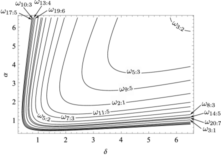
Figure 4: Examples of resonance curves plotted on the parameter plane for fixed $\beta=1$

Limiting the normalization of the Hamiltonian $H$ (3.2) only to the quadratic part ${\mathscr{H}}_{2}$, does not give in general sufficient accuracy of solutions of Hamilton’s equations of the original untruncated $H$. Thus, in order to improve the accuracy we need to take into account the higher order terms of $H$, and normalize them so that the Hamiltonian and the dynamics become especially simple. We can do this by means of a sequence of nonlinear canonical transformations with some appropriately chosen generating function

$$S=\boldsymbol{P}^{T}\boldsymbol{q}+W(\boldsymbol{q},\boldsymbol{P}),\qquad W=W_{3}+\dots+W_{K},$$ (3.19)

where

$$W_{K}=\sum_{\nu_{1}+\dots+\mu_{n}=K}w_{\nu_{1},\dots\mu_{n}}q_{1}^{\nu_{1}}\cdots q_{n}^{\nu_{n}}P_{1}^{\mu_{1}}\cdots P_{n}^{\mu_{n}},$$

for details consult e.g., [3, 2]. Let

$$\boldsymbol{Q}=\dfrac{\partial S}{\partial\boldsymbol{P}}=\boldsymbol{q}+\dfrac{\partial W(\boldsymbol{q},\boldsymbol{P})}{\partial\boldsymbol{P}},\qquad\boldsymbol{p}=\dfrac{\partial S}{\partial\boldsymbol{q}}=\boldsymbol{P}+\dfrac{\partial W(\boldsymbol{q},\boldsymbol{P})}{\partial\boldsymbol{q}}$$ (3.20)

be the canonical transformation generated by (3.19). Then, from the implicit function theorem, in the neighborhood on the equilibrium $\boldsymbol{X}=0$ we can express $(\boldsymbol{q},\boldsymbol{p})$ as a functions of $(\boldsymbol{Q},\boldsymbol{P})$. Namely, one can solve (3.20) for $\boldsymbol{q}$ and $\boldsymbol{p}$, treating the derivatives as known, and then recursively substitute those expressions into themselves. Because $W$ contains polynomials of degree 3 or higher, the Taylor series is recovered, with the first terms

$$\boldsymbol{q}=\boldsymbol{Q}-\dfrac{\partial W(\boldsymbol{Q},\boldsymbol{P})}{\partial\boldsymbol{P}}+\dots,\qquad\boldsymbol{p}=\boldsymbol{P}+\dfrac{\partial W(\boldsymbol{Q},\boldsymbol{P})}{\partial\boldsymbol{Q}}+\dots.$$ (3.21)

The Hamiltonian function in the new variables is reduced to the Birkhoff normal form ${\mathcal{H}}_{K}(\boldsymbol{X})$ of order $K$, i.e., with all homogeneous terms of degrees up to $K$ normalized so that they Poisson commute with the quadratic part

$$H(\boldsymbol{x})={\mathcal{H}}_{K}(\boldsymbol{X})+{\mathcal{O}}(\boldsymbol{X}^{K+1}),\quad\{{\mathcal{H}}_{K},{\mathcal{H}}_{2}\}=0.$$ (3.22)

Introducing the action-angle variables as the symplectic polar coordinates $(I_{i},\phi_{i})$ defined by

$$Q_{i}=\sqrt{2I_{i}}\sin\phi_{i},\qquad P_{i}=\sqrt{2I_{i}}\cos\phi_{i},\qquad i=1,\dots,n$$

and discarding the non-normalized terms in (3.22) we obtain the integrable system whose Hamiltonian ${\mathcal{H}}_{K}(\boldsymbol{I})$ depends only on actions and whose trajectories will round the tori $\boldsymbol{I}=\operatorname{const}$ with frequencies $\boldsymbol{\Omega}=\partial_{\boldsymbol{I}}{\mathcal{H}}_{K}$. Since ${\mathcal{H}}_{K}(\boldsymbol{X})$ consist of homogeneous terms of degrees up to $K$ its Birkhoff normal form can be written in action-angle variables as a polynomial of degree $[K/2]$ in $\boldsymbol{I}$. We can transform $H$ to such form by a sequence of canonical transformations provided eigenfrequences $\omega_{i}$ do not satisfy any resonance relation of order $K$ or less.

The Birkhoff normal form of degree four is given by

$${\mathcal{H}}_{4}=\omega_{1}I_{1}+\omega_{2}I_{2}+h_{20}I_{1}^{2}+h_{11}I_{1}I_{2}+h_{02}I_{2}^{2},$$ (3.23)

where the coefficients $h_{20},h_{11},h_{02}$ related to our system have the form

$$\begin{split}h_{20}&=\frac{\omega_{1}^{2}\omega_{2}^{4}\left(\omega_{1}^{2}-1\right)\left(3\delta\left(\omega_{1}^{2}-1\right)\left(\omega_{2}^{2}-1\right)+\left(3\omega_{2}^{2}+1\right)\omega_{1}^{2}-3\omega_{2}^{2}+3\right)}{16\delta^{2}\left(\omega_{1}^{2}-\omega_{2}^{2}\right)^{2}\left(\omega_{2}^{2}-1\right)},\\ h_{11}&=\frac{\omega_{1}^{3}\omega_{2}^{3}\left(\left(1-3\omega_{2}^{2}\right)\omega_{1}^{2}+\omega_{2}^{2}-3-3\delta\left(\omega_{1}^{2}-1\right)\left(\omega_{2}^{2}-1\right)\right)}{4\delta^{2}\left(\omega_{1}^{2}-\omega_{2}^{2}\right)^{2}},\\ h_{02}&=\frac{\omega_{1}^{4}\omega_{2}^{2}\left(\omega_{2}^{2}-1\right)\left(3\delta\left(\omega_{1}^{2}-1\right)\left(\omega_{2}^{2}-1\right)+3\left(\omega_{2}^{2}-1\right)\omega_{1}^{2}+\omega_{2}^{2}+3\right)}{16\delta^{2}\left(\omega_{1}^{2}-1\right)\left(\omega_{1}^{2}-\omega_{2}^{2}\right)^{2}}.\end{split}$$ (3.24)

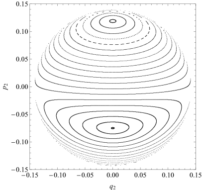
(a) Numerical

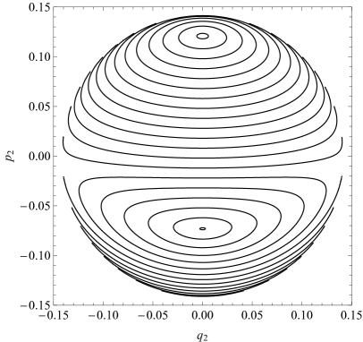
(b) Analytical

Figure 5: Poincaré sections on the surface $q_{1}=0$, with $p_{1}>0$

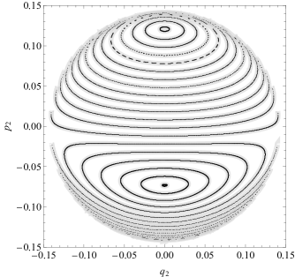
Figure 6: Superposition of Figs. 5(a)-(b)

Now let us try to deduce some interesting information from the normalized Hamiltonian (3.23). First of all, in order to check that the normalization up to order four gives sufficiently good accuracy, we have to compare solutions of Hamilton equations governed by Hamiltonian (3.23) with (3.2). We can do this easily for example by comparison of Poincaré cross sections for original Hamiltonian system and its normal form of degree four. Let us note that action variables $(I_{1},I_{2})$ are the first integrals of the normalized Hamiltonian ${\mathcal{H}}_{4}$. We can chose one of them, for example $I_{1}$ and make the inverse canonical transformation in order to go back to the original variables $(q_{1},q_{2},p_{1},p_{2})^{T}$. Then for the chosen energy level we make the contour plot of $I_{1}$ restricted to the plane $(q_{2},p_{2})$ with $q_{1}=0$. Figure 5 presents numerical and analytical Poincaré cross sections constructed for chosen values of parameters belonging to the stability region, namely: $\omega_{1}=\omega_{1}=1.75,\ \omega_{2}=0.5,\ \delta=0.75,$ with cross-section plane $q_{1}=0$ and $p_{1}>0$, on the energy level $E=E_{\text{min}}+0.01$. As expected, for $E$ close to the energy minimum corresponding to an equilibrium both the images are very regular. In fact each of them can be divided into two regions filled by invariant tori around two stable particular periodic solutions. As we can notice, the differences between numerical and analytical computations are not visible. See especially the Figure 6 showing the superposition of Figures 5(a)-(b), where for better readability the analytical loops have been plotted in bold gray lines.

As we mentioned previously, the Birkhoff normalization can be also very effective in finding families of periodic solutions. Figures 7-9 present contour plots showing examples of such families

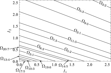
Figure 7: Contour plot showing the resonance curves on the $(I_{1},I_{2})$ plane for the fixed values of parameters: $\omega_{1}=1.75,\ \omega_{2}=0.5,\ \delta=0.75$

• on the $(I_{1},I_{2})$ plane,

• on the $(q_{1},q_{2})$ plane with $p_{1}=p_{2}=0$,

• on the $(q_{2},p_{2})$ plane with $q_{1}=p_{1}=0$,

respectively, where $(\Omega_{1},\Omega_{2})$ are defined by

$$\begin{split}\Omega_{1}=\dfrac{\partial{\mathcal{H}}_{4}}{\partial I_{1}}&=\omega_{1}+2h_{20}I_{1}+h_{11}I_{2},\quad\Omega_{2}=\dfrac{\partial{\mathcal{H}}_{4}}{\partial I_{2}}=\omega_{1}+2h_{02}I_{2}+h_{11}I_{1},\\ &\quad\text{and}\quad\Omega_{n:m}:=\left\{(I_{1},I_{2})\in\mathbb{R}^{2}\ \Big{|}\ \frac{\Omega_{1}}{\Omega_{2}}=\frac{n}{m}\right\}.\end{split}$$ (3.25)

These figures are very helpful because from them we can read initial conditions conditions for which the motion of the system is periodic. For example, Figure 10 presents periodic orbits in the configuration space given by the numerical computations with the initial values related to resonances $\Omega_{17:5}$ and $\Omega_{10:3}$ respectively.

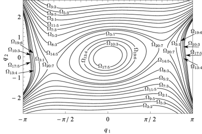
Figure 8: Contour plot showing the resonance curves on the $(q_{1},q_{2})$ plane with $p_{1}=p_{2}=0$ for the fixed values of parameters: $\omega_{1}=1.75,\ \omega_{2}=0.5,\ \delta=0.75$

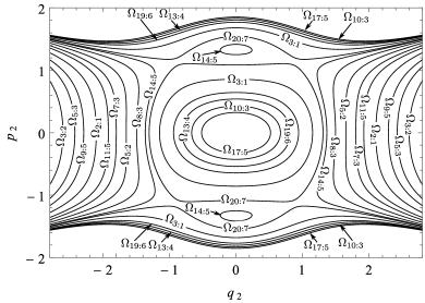
Figure 9: Contour plot showing the resonance curves on the $(q_{2},p_{2})$ plane with $q_{1}=p_{1}=0$ for the fixed values of parameters: $\omega_{1}=1.75,\ \omega_{2}=0.5,\ \delta=0.75$

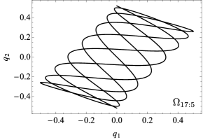
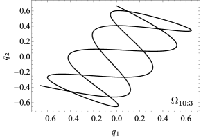
Figure 10: Examples of trajectories in the configuration space given by the numerical computations with the initial values related to certain resonances presented in Figs. 8-9

4 Conclusions

As we have seen, in order to determine stability of equilibrium solution, detect families of periodic solutions as well as find approximation of analytic solutions of equations of motion the Birkhoff normalization proves very useful. However, it is worth mentioning certain inconveniences associated with this method. Namely, it gives us opportunity to investigate behavior of the system over large time intervals, with sufficiently good accuracy, only in the neighborhood of equilibrium. Furthermore, it should be emphasized that the linear stability of the equilibrium $\boldsymbol{x}=0$ does not imply its stability in the Lyapunov sense. This is due to the fact that the discarded parts of the series can destroy the stability in the long timescale. It would seem that the higher degree normalization should gives us a better approximation of reality. However, in general there does not exist a convergent Birkhoff transformation, see e.g., [6], so the estimation of those terms is not straightforward. To check the non-linear stability of equilibrium for Hamiltonian vector field $\boldsymbol{v}_{H}(\boldsymbol{x})$ more involved analysis is necessary, e.g., application of the second Lyapunov method or the Arnold-Moser theorem, which itself relies on normal form, see [4].

Despite these limitations, the Birkhoff normalization is still a very useful source of important information about dynamics and often the starting point of further analysis.

References

• [1] Birkhoff, G. D.: Dynamical Systems. American Math Society (1927)
• [2] Jorba, Á.: A Methodology for the Numerical Computation of Normal Forms, Centre Manifolds and First Integrals of Hamiltonian Systems. Experimental Mathematics. 8, 155–195 (1999)
• [3] Markeev, A. P.: Libration Points in Celestial Mechanics and Cosmodynamics, Nauka, Moscow (1978), In Russian
• [4] Merkin, D. R.: Introduction to the Theory of Stability, Texts in Applied Mathematics, 24, Springer-Verlag, New York (1997)
• [5] Morales-Ruiz, J. J.: Differential Galois Theory and Non-Integrability of Hamiltonian Systems, Progress in Mathematics, Birkhauser Verlag, Basel (1999)
• [6] Perez-Marco, R.: Convergence or generic divergence of the Birkhoff normal form. Ann. of Math. 157, 557–574 (2003)
• [7] Szumiński, W., Przybylska, M.: Non-integrability of constrained n-body problems with Newton and Hooke interactions. Work in progress
• [8] Van der Put, M., Singer, M. F.: Galois theory of linear differential equations, Springer-Verlag, Berlin (2003)