Comprehending Isospin breaking effects of $X(3872)$ in a Friedrichs-model-like scheme

Abstract

Recently, we have shown that the $X(3872)$ state can be naturally generated as a bound state by incorporating the hadron interactions into the Godfrey-Isgur quark model using the Friedrichs-like model combined with the QPC model, in which the wave function for the $X(3872)$ as a combination of the bare $c\bar{c}$ state and the continuum states can also be obtained. Under this scheme, we now investigate the isospin breaking effect of $X(3872)$ in its decays to $J/\psi\pi^{+}\pi^{-}$ and $J/\psi\pi^{+}\pi^{-}\pi^{0}$. By Considering its dominant continuum parts coupling to $J/\psi\rho$ and $J/\psi\omega$ through the quark rearrangement process, one could obtain the reasonable ratio of $\mathcal{B}(X(3872)\rightarrow J/\psi\pi^{+}\pi^{-}\pi^{0})/\mathcal{B}(X(3872)\rightarrow J/\psi\pi^{+}\pi^{-})\simeq(0.58\sim 0.92)$. It is also shown that the $\bar{D}D^{*}$ invariant mass distributions in the $B\rightarrow\bar{D}D^{*}K$ decays could be understood qualitatively at the same time. This scheme may provide more insight to understand the enigmatic nature of the $X(3872)$ state.

I Introduction

The enigmatic $X(3872)$ state has been highlighted for more than one decade, after it was first discovered by Belle Choi et al. (2003) and confirmed by CDF, D0, and BABAR Acosta et al. (2004); Abazov et al. (2004); Aubert et al. (2005). The mass of the $X(3872)$ is at $3871.69\pm 0.17$ MeV Patrignani et al. (2016), almost degenerate with the $D^{*0}\bar{D}^{0}$ threshold, which is the most intriguing feature. Its width is also very narrow, with an upper limit $1.2\ \mathrm{MeV}$. Its quantum number is determined to be $J^{PC}=1^{++}$ by LHCb Aaij et al. (2013), which is consistent with its radiative decay Bhardwaj et al. (2011); Aubert et al. (2006); Bhardwaj et al. (2011) and multi-pion transitions Abulencia et al. (2006); del Amo Sanchez et al. (2010). The negative result in searching for its charged partner in $B$ decays Aubert et al. (2005) implies that it should be an isoscalar state. Nevertheless, the dominant $\rho$ contribution of dipion mass spectrum in $X(3872)\rightarrow J/\psi\pi^{+}\pi^{-}$ Acosta et al. (2004) suggests a large isospin breaking effect. Compared with its decay to $J/\psi\pi^{+}\pi^{-}\pi^{0}$ through the I=0 $\omega$ resonance, the ratio is measured to be

$$\frac{\Gamma(X(3872)\rightarrow J/\psi\pi^{+}\pi^{-}\pi^{0})}{\Gamma(X(3872)\rightarrow J/\psi\pi^{+}\pi^{-})}=1.0\pm 0.4\pm 0.3$$ (1)

by Belle Abe et al. (2005) and

$$\frac{\Gamma(X(3872)\rightarrow J/\psi\pi^{+}\pi^{-}\pi^{0})}{\Gamma(X(3872)\rightarrow J/\psi\pi^{+}\pi^{-})}=0.8\pm 0.3$$ (2)

by BABAR del Amo Sanchez et al. (2010). These characteristics and other properties as discussed in the literatures (see refs. Guo et al. (2017); Chen et al. (2016); Esposito et al. (2017); Lebed et al. (2017) for example) suggest an exotic nature of the $X(3872)$ .

The proximity of the $X(3872)$ to the $D^{*0}\bar{D}^{0}$ threshold leads to a direct interpretation of it as a hadronic molecular state. In fact, Törnqvist predicted a similar $D\bar{D}^{*}$ bound state around $3870$MeV about ten years before the discovery of the $X(3872)$Tornqvist (1994), using a pion exchange model similar to the discussion of the Deuteron in the $pn$ system, and named the state as a “deuson”. However, this picture may not explain the production cross section of $X(3872)$ in $p\bar{p}$ annihilation Bignamini et al. (2009) and also can not explain its large decay rate to $\gamma\psi^{\prime}$ Swanson (2004); Dong et al. (2011). This meson-exchange model is also extended to include other intermediate hadronic states like $\sigma$, $\rho$ and $\omega$ in Ref. Liu et al. (2008, 2009); Li and Chao (2009). The tetraquark model is also introduced to explain its existence and the other exotic statesMaiani et al. (2005). However, this explanation also meets the large $\gamma\psi^{\prime}$ decay rate problem. This bound state can also be reproduced by other models, such as the effective Lagrangian approach AlFiky et al. (2006); Fleming et al. (2007), chiral unitary calculation Wang and Wang (2013), screened potential model Li and Chao (2009) and coupled-channel model Zhou and Xiao (2014). It was also pointed out in Braaten and Lu (2007); Coito et al. (2013) that $X(3872)$ could be a mixture of a $c\bar{c}$ and the molecule-like $D\bar{D}^{*}$ components which may provide both solution to the production and the radiative decay problem. In our recent work Zhou and Xiao (2017), we discussed the first exited $P$-wave charmonium states using a Friedrichs-like model combined with the quark pair creation (QPC) model Micu (1969); Blundell and Godfrey (1996) to incorporate the hadron interaction effect into the Godfrey-Isgur (GI) quark model. We found that in the $2^{3}P_{1}$ channel the $X(3872)$ could be naturally generated as a bound state just below the $D^{0}\bar{D}^{0*}$ threshold in this framework, while another resonance pole at around $3.934\pm 0.040i$GeV on the Riemann sheet attached to the physical region above the $\bar{D}D^{*}$ threshold is found to be generated from the bare $\chi_{c1}(2P)$, which might be related to the observed $X(3940)$ state in the experiment. Compared to the above “deuson” picture, in this scheme, similar to Ref. Braaten and Lu (2007); Coito et al. (2013), the $X(3872)$ is dynamically generated by the coupling of the bare ${2}^{3}P_{1}$ $c\bar{c}$ state with the continuum, not from the pion exchange. The wave function of $X(3872)$ can also be explicitly written down as a linear combination of $c\bar{c}$ and the continuum states. With this information, more properties of the $X(3872)$ can be studied. In this paper, we will mainly focus on the isospin breaking effect based on this result.

The ratio ${\Gamma(X(3872)\rightarrow J/\psi\pi^{+}\pi^{-}\pi^{0})}/{\Gamma(X(3872)\rightarrow J/\psi\pi^{+}\pi^{-})}$ seems to imply a significant isospin breaking effect, but it is first pointed out by Suzuki that it might be misleading Suzuki (2005). Because the central mass value of $J/\psi\omega$ is about 7 MeV higher than the $X(3872)$ mass, while the central value of $J/\psi\rho$ energy is lower than the $X(3872)$ mass, the $\pi^{+}\pi^{-}\pi^{0}$ in the $J/\psi\pi^{+}\pi^{-}\pi^{0}$ final state comes from the far tail of the $\omega$ resonance and the kinematical phase space of the isospin-conserved process is highly suppressed. Considering this kinematical constraint, the production amplitude ratio $\frac{A(X(3872)\rightarrow J/\psi\rho)}{A(X(3872\rightarrow J/\psi\omega))}$ is estimated to be $0.27\pm 0.02$ to produce a comparable result with the experiment. Meng and Chao addressed this problem by considering the rescattering effect in an effective lagrangian method Meng and Chao (2007). They treated the $X(3872)$ as an elementary field and introduced the effective interactions among the $X$ state, the pseudoscalar, and the vector mesons. By calculating the imaginary and real part of the rescattering amplitudes, they found a consistent value of the ratio in their parameter space. Li and Zhu Li and Zhu (2012) investigated the probability in the framework of one-meson-exchange with considering the S-D wave mixing and they obtained the ratio of these two modes to be 0.42. Gammermann and Oset Gamermann and Oset (2009) used the on-mass-shell Lippmann-Shwinger equation method and found a branch ratio of 1.4.

In the present paper, as stated above, we will discuss the isospin-breaking effect from the starting point of our previous paper Zhou and Xiao (2017). The Friedrichs-like model is exactly solvable and the interactions between the bare $c\bar{c}$ and the Okubo-Zweig-Iizuka (OZI) allowed continuum states are approximated by the QPC model using the wave functions for bare states from the GI model. This just provides a general scheme to make corrections to the well-accepted GI model by including the hadron interactions. The experimentally observed first excited $P$-wave charmonium states can be reasonably produced simultaneously. The wave functions for these states in terms of the bare $c\bar{c}$ and continuum states can also be explicitly written down. Once the wave function of the $X(3872)$ is explicitly given in this scheme, we are able to insert an interaction Hamiltonian between the $X(3872)$ wave function and the final states $J/\psi\omega$ or $J/\psi\rho$ and calculate the related transition amplitudes and the branching fraction. If the OZI suppressed couplings are omitted, the $c\bar{c}$ contribution would be neglected and only the continuum components will contribute to the amplitude. The couplings between the final states and the continuum parts could then be described by the quark rearrangement model developed by Barnes and Swanson (BS model) Barnes and Swanson (1992). The merit of this choice is that the BS model considers the spin-spin hyperfine, color Coulomb, and linear confinement interactions among the quarks between different mesons, which respects the same spirit as the GI model and no new parameter needs to be introduced. By a standard derivation of the representation of transition amplitude and numerical calculations, our final result of $\frac{\Gamma(X(3872)\rightarrow J/\psi\pi^{+}\pi^{-}\pi^{0})}{\Gamma(X(3872)\rightarrow J/\psi\pi^{+}\pi^{-})}$ turns out to be in good agreement with the experiment value. Our method may have some similarity with the widely used coupled-channel formalism such as Eichten et al. (1978); Kalashnikova (2005); Ortega et al. (2010); Takizawa and Takeuchi (2013). However, we are using the well-accepted GI’s wave function in the QPC model and the quark rearrangement model in our calculation, which provides more solid theoretical basis and makes our result more convincing.

This paper is organized as follows: The theoretical foundations are introduced in Section II, which include the Friedrichs model, its extended scheme, and the quark rearrangement model by Barnes and Swanson. The numerical calculations of the isospin breaking effect are given in Section III. Section IV is the final conclusion and discussions.

II Theoretical model

In this section, we will briefly introduce the theoretical basis of our discussion which includes the main results of the Friedrichs model and its extended version, the quark rearrangement model by Barnes and Swanson, and the derivations of the transition amplitudes of $X(3872)$ to $J/\psi\omega$ or $J/\psi\rho$.

II.1 The Friedrichs model

In 1948, Friedrichs proposed an exactly solvable model to understand an unstable state Friedrichs (1948). The simplest form of Friedrichs model includes a free Hamiltonian $H_{0}$ and an interaction part $V$. The free Hamiltonian $H_{0}$ has a bare continuous spectrum $[E_{th},\infty)$, and a discrete eigenvalue $E_{0}$ imbedded in this continuous spectrum ($E_{0}>E_{th}$). The interaction part describes the coupling between the bare continuous state and discrete states of $H_{0}$ so that the discrete state is dissolved in the continuous state and a resonance is produced.

In the energy representation, the free Hamiltonian can be expressed as

$$H_{0}=E_{0}|0\rangle\langle 0|+\int_{E_{th}}^{\infty}E|E\rangle\langle E|\mathrm{d}E,$$ (3)

where $|0\rangle$ denotes the bare discrete state and $|E\rangle$ denotes the bare continuum state. The normalization conditions for the bare states are

$$\langle 0|0\rangle=1,\langle E|E^{\prime}\rangle=\delta(E-E^{\prime}),\langle 0|E\rangle=\langle E|0\rangle=0.$$ (4)

The interaction part serves to couple the bare discrete state and the bare continuous state as

$$V=\lambda\int_{E_{th}}^{\infty}\big{[}f(E)|E\rangle\langle 0|+f^{*}(E)|0\rangle\langle E|\big{]}\mathrm{d}E,$$ (5)

where $f(E)$ function denotes the coupling function and $\lambda$ the coupling strength. This eigenvalue problem $H\Psi(x)=x\Psi(x)$, with the full Hamiltonian $H=H_{0}+V$, can be exactly solved and the final continuum state is

$$|\Psi_{\pm}(x)\rangle = |x\rangle+\lambda\frac{f^{*}(x)}{\eta^{\pm}(x)}\Big{[}|0\rangle+\lambda\int_{E_{th}}^{\infty}\frac{f(E)}{x-E\pm i\epsilon}|E\rangle\mathrm{d}E\Big{]},$$ (6)

in which the resolvent $\eta^{\pm}(x)$ is defined as

$$\eta^{\pm}(x)=x-E_{0}-\lambda^{2}\int_{E_{th}}^{\infty}\frac{|f(E)|^{2}}{x-E\pm i\epsilon}\mathrm{d}E\,.$$ (7)

The normalization is $\langle\Psi_{\pm}(E)|\Psi_{\pm}(E^{\prime})\rangle=\delta(E-E^{\prime})$ and the subscript $\pm$ denotes the in-states ($+$) and out-states ($-$), respectively. The scattering $S$-matrix can also be obtained as

$$S(E,E^{\prime})=\delta(E-E^{\prime})\Big{(}1-2\pi i\frac{\lambda f(E)f^{*}(E)}{\eta^{+}(E)}\Big{)}.$$ (8)

The $\eta^{\pm}$ functions can be analytically continued to the complex $z$-plane to be one complex function $\eta(z)$ for $z\in\mathbb{C}$ with its boundary values $\eta(x\pm i\epsilon)=\eta^{\pm}(x)$ on the real axis. Since there is only one threshold for the continuum, there is only one cut for this function, and the $\eta(z)$ function is defined on a two-sheeted Riemann surface. The zero points for the $\eta(z)=0$ will be the poles for the $S$-matrix. The zero points of $\eta(z)$ or the poles of the $S$-matrix will represent the generalized complex-valued eigenstates (called Gamow state) for the full Hamiltonian, which satisfy $H|z\rangle=z|z\rangle$ with $z\in\mathbb{C}$ as described in the Rigged-Hilbert-Space (RHS) formulation of the quantum mechanics developed by Bohm and Gadella Bohm and Gadella (1989); Civitarese and Gadella (2004). By summing all the perturbation series, Prigogine and his collaborators also obtained a similar mathematical description Petrosky et al. (1991). In general, the different kinds of the generalized eigenstates are summarized in the following:

1. Bound state:

   The solution of $\eta(z)=0$ on the first-sheet real axis below $E_{th}$ represents a bound state. Its wave function is written down as

   $$|z_{B}\rangle=N_{B}\Big{(}|0\rangle+\lambda\int_{E_{th}}^{\infty}\frac{f(E)}{z_{B}-E}|E\rangle\mathrm{d}E\Big{)},$$ (9)

   This solution has a finite norm and can be normalized as $\langle z_{B}|z_{B}\rangle=1$ where

   $$N_{B}=(\eta^{\prime}(z_{B}))^{-1/2}=\Big{(}1+\lambda^{2}\int\mathrm{d}E\frac{|f(E)|^{2}}{(z_{B}-E)^{2}}\Big{)}^{-1/2}.$$ (10)

   Then, it is straightforward to define the so-called “elementariness” $Z$ and “compositeness” $X$ as

   $$Z=\frac{1}{N_{B}^{2}},\,\,\,\,X=\frac{\lambda^{2}}{N_{B}^{2}}\int\mathrm{d}E\frac{|f(E)|^{2}}{(z_{B}-E)^{2}}$$ (11)

   similar to the ones in the Weinberg’s pioneering work in studying the compositeness of deuteron Weinberg (1963). The physical meanings of the “elementariness” and “compositeness” are the probabilities of finding the bare discrete and the bare continuum states in the bound state respectively.

2. Virtual state:

   The solution lying on the real axis of the second Riemann sheet below the threshold represents a virtual state. Its wave function is expressed as

   $$|z^{\pm}_{V}\rangle=N_{V}\Big{(}|0\rangle+\lambda\int_{E_{th}}^{\infty}\frac{f(E)}{z_{V}^{\pm}-E}|E\rangle\mathrm{d}E\Big{)},$$ (12)

   where the superscript $\pm$ denotes the two kinds of integration contours which are continued from the first sheet to the second sheet to enclose the virtual state pole from the upper side (+) or the lower side (-) of the first sheet cut Xiao and Zhou (2016). Unlike the bound state, a virtual state does not have a well-defined norm as the usual state in the Hilbert space. Thus the compositeness and the elementariness for a virtual state can not be mathematically rigorously defined. However, we can define a normalization such that $\langle z_{V}^{-}|z_{V}^{+}\rangle=1$, by choosing

   $$N_{V}=(\eta^{\prime}(z_{V}))^{-1/2}=\Big{(}1+\lambda^{2}\int\mathrm{d}E\frac{|f(E)|^{2}}{(z_{V}-E)^{2}}\Big{)}^{-1/2}.$$ (13)

   One typical example is the virtual state in the singlet neutron-proton scattering, which serves to contribute to the unusually large scattering length.

3. Resonant state:

   The real analyticity of the $\eta(z)$ function requires the solutions of $\eta(z)=0$ on the second complex energy plane to appear as a conjugate pair. This pair of poles of $S$-matrix represents a resonance since it will be unstable for its finite imaginary part of the energy eigenvalue. The pole position on the lower-half energy plane of the second Riemann sheet is related to the mass $M$ and width $\Gamma$ as $z_{R}=M-i\frac{\Gamma}{2}$. The wave functions for them is written as

   $$|z_{R}\rangle=N_{R}\Big{(}|0\rangle+\lambda\int_{E_{th}}^{\infty}\mathrm{d}E\frac{f(E)}{[z_{R}-E]_{+}}|E\rangle\Big{)},$$

   $$|z_{R}^{*}\rangle=N_{R}^{*}\Big{(}|0\rangle+\lambda\int_{E_{th}}^{\infty}\mathrm{d}E\frac{f^{*}(E)}{[z_{R}^{*}-E]_{-}}|E\rangle\Big{)},$$ (14)

   where $z_{R}$ is on the lower half plane and $z_{R}^{*}$ is its complex conjugate. The $[\cdots]_{\pm}$ means the analytical continuations of the integrations from upper or lower edge of the first sheet cut Xiao and Zhou (2016). Similar to the virtual state, the wave function of a resonant state can not be normalized as usual, and thus is not the normal state vector in the Hilbert space. However we can choose

   $$N_{R}=(\eta^{\prime+}(z_{R}))^{-1/2}=\Big{(}1+\lambda^{2}\int\mathrm{d}E\frac{|f(E)|^{2}}{[(z_{R}-E)_{+}]^{2}}\Big{)}^{-1/2}$$ (15)

   to normalize the state as $\langle z_{R}^{*}|z_{R}\rangle=1$ and similarly for the $|z_{R}^{*}\rangle$. The normalization factor $N_{R}$ will be complex in general and one might define “elementariness” and “compositeness” parameters as in Ref. Xiao and Zhou (2017), but their physical meanings are not clear because they are complex numbers too. However, some other physical approximate definitions proposed in Ref. Sekihara et al. (2015); Guo and Oller (2016) might be used to describe these quantities.

It is worth emphasizing that these discrete spectrum solutions may or may not be generated from the bare discrete state of the free Hamiltonian. If the state is generated from the bare discrete state, it will move back to the bare state as one decreases the coupling strength to zero. Besides, the discrete state could also be dynamically generated from the singularities of the form factor. In this occasion, if the coupling strength is tuned to be zero, the positions of this kind of state may move towards the singularity of the form factor on the unphysical sheets Xiao and Zhou (2016, 2017). It is also worth mentioning that the Friedrichs model has several variants such as the Fano model Fano (1961), the Lee model Lee (1954), the Anderson model Anderson (1961) in other physics areas.

II.2 The extended Friedrichs model and the QPC model

In the original Friedrichs model, the states are labeled only by the energy quantum number which seems to be unrelated to the states in the three dimensional space. In fact, after partial-wave decomposition of the three dimensional states, the similar model in terms of the angular momentum eigenstate is reduced to a Friedrichs-like model Xiao and Zhou (2017). Consider the coupling of a bare discrete state $|0,JM\rangle$ with a spin quantum number $J$ and the magnetic quantum number $M$ and the bare continuum momentum eigenstate $|\vec{p},S,S_{z}\rangle$ with a total spin $S$, $z$-component $S_{z}$, and $\pm\vec{p}$ the c.m. momentum for the two particles composing the continuum state for example. The discrete state denoted by the total Hamiltonian for fixed $JM$ can be recast into

$$H= M_{0}|0\rangle\langle 0|+\sum_{L}\int\mathrm{d}E\,E|E,L\rangle\langle E,L|+\sum_{L}\int\mathrm{d}Ef_{L}(E)|0\rangle\langle E,L|+h.c.$$ (16)

in which $|0\rangle=|0;JM\rangle$, $|E,L\rangle=\sqrt{\mu p}|p;JM;LS\rangle$ with $\mu$ the reduced mass of the two-particle state in its $c.m.$ frame and $f(E)$ the coupling form factor, as derived in Ref. Xiao and Zhou (2017). This is just similar to the original Friedrichs model but with more continuum and the similar exact solution can be obtained.

We can make more generalization by adding more discrete states and more continuum states, and the interactions between continuum states can also be introduced. The most general Hamiltonian with $D$ discrete states, $|i\rangle$ ($i=1,\dots,D$), and $C$ continuum states, $|E_{j},j\rangle$ ($j=1,\dots,C$), can be expressed as

$$H= \sum_{i=1}^{D}M_{i}|0;i\rangle\langle 0;i|+\sum_{i=1}^{C}\int_{M_{i,th}}^{\infty}\mathrm{d}E_{i}E_{i}|E_{i};i\rangle\langle E_{i};i|$$

$$+\sum_{i_{2},i_{1}}\int_{M_{i_{1},th}}\mathrm{d}E^{\prime}\,\int_{M_{i_{2},th}}\mathrm{d}E\,g_{i_{2},i_{1}}(E^{\prime},E)|E^{\prime};i_{2}\rangle\langle E;i_{1}|+h.c.$$

$$+\sum^{D}_{i=1}\sum_{j=1}^{C}\int_{M_{j,th}}\mathrm{d}Ef_{i,j}(E)|0;i\rangle\langle E;j|+h.c.$$ (17)

where $f_{i,j}(E)$ is the form factor describing the interaction between the $i$th discrete state and the $j$th continuum state, and $g_{ij}$ describes the interaction between the $i$th continuum and the $j$th continuum. For general interactions $g_{ij}$, the model is not solvable, but if $g_{ij}(E^{\prime},E)=v_{ij}f_{i}(E^{\prime})f_{j}(E)$ and $f_{ij}=u_{ij}f_{j}(E)$, where $u_{ij}$ and $v_{ij}$ are constant, the model can also be exactly solved. See Ref. Xiao and Zhou (2017) for details.

In the present study, we only consider the case where only one discrete states is coupled with several continuum states without the interactions between the continuum states. The solutions differ from the ones previously described by simply adding more similar continuum integrals in Eqs. (7), (9), (12), (14).

We will restrict our study on the properties of mesons. The next problem is to determine the interaction between one meson state and the two meson continuum states, $i.e.$ the coupling form factor in the Friedrichs model. A simple method is to use the QPC model Micu (1969); Blundell and Godfrey (1996) to describe the interaction of one meson and two-meson continuum states.

In this model, the meson coupling $A\rightarrow BC$ can be defined as the transition matrix element

$$\langle BC|T|A\rangle=\delta^{3}(\vec{P_{f}}-\vec{P_{i}})\mathcal{M}^{ABC}$$ (18)

where the transition operator $T$ in the QPC model is defined as

$$T=-3\gamma\sum_{m}\langle 1m1-m|00\rangle\int\mathrm{d}^{3}\vec{p_{3}}\mathrm{d}^{3}\vec{p_{4}}\delta^{3}(\vec{p_{3}}+\vec{p_{4}})\mathcal{Y}_{1}^{m}(\frac{\vec{p_{3}}-\vec{p_{4}}}{2})\chi_{1-m}^{34}\phi_{0}^{34}\omega_{0}^{34}b_{3}^{\dagger}(\vec{p_{3}})d_{4}^{\dagger}(\vec{p_{4}}),$$ (19)

describing a quark-antiquark pair generated by the $b^{\dagger}_{3}$ and $d^{\dagger}_{4}$ creation operators from the vacuum. $\phi_{0}^{34}=(u\bar{u}+d\bar{d}+s\bar{s})/\sqrt{3}$ is the $SU(3)$ flavor wave function for the quark-antiquark pair. $\chi^{34}_{1-m}$ and $\omega^{34}_{0}$ are the spin wave function and the color wave function, respectively. $\mathcal{Y}_{1}^{m}$ is the solid Harmonic function. $\gamma$ parameterizes the production strength of the quark-antiquark pair from the vacuum. The definition of the meson state here is different from the one in Ref. Hayne and Isgur (1982) by omitting the factor $\sqrt{2E}$ to ensure the correct normalizations in the Friedrichs-like model, as

$$|A(n,{}^{2S+1}L_{J,M})(\vec{P})\rangle= \sum_{M_{L},M_{S}}\langle LM_{L}SM_{S}|JM\rangle\int\mathrm{d}^{3}p\,\psi_{nLM_{L}}(\vec{p})\,\chi^{12}_{SM_{S}}\,\phi^{12}\,\omega^{12}$$

$$\times\Big{|}q_{1}\Big{(}\frac{m_{1}}{m_{1}+m_{2}}\vec{P}+\vec{p}\Big{)}\bar{q}_{2}\Big{(}\frac{m_{2}}{m_{1}+m_{2}}\vec{P}-\vec{p}\Big{)}\Big{\rangle}.$$

$\chi^{12}$, $\phi^{12}$ and $\omega^{12}$ are the spin wavefunction, flavor wave function and the color wave function, respectively. $p_{1}$ ($p_{2}$) and $m_{1}$ ($m_{2}$) are the momentum and mass of the quark (anti-quark). $\vec{P}=\vec{p}_{1}+\vec{p}_{2}$ is the momentum of the center of mass, and $\vec{p}=\frac{m_{2}\vec{p}_{1}-m_{1}\vec{p}_{2}}{m_{1}+m_{2}}$ is the relative momentum. $\psi_{nLM_{L}}$ is the wave function for the meson, $n$ being the radial quantum number.

By the standard derivation one can obtain the amplitude $\mathcal{M}^{ABC}$ defined by Eq. (18) and the partial-wave amplitude $\mathcal{M}^{SL}(P(E))$ as in Ref. Blundell and Godfrey (1996). Then the form factor $f_{SL}$ which describes the interaction between $|A\rangle$ and $|BC\rangle$ in the Friedrichs model can be obtained as

$$f_{SL}(E)=\sqrt{\mu P(E)}\mathcal{M}^{SL}(P(E)),$$ (20)

where $P(E)=$$\sqrt{\frac{2M_{B}M_{C}(E-M_{B}-M_{C})}{M_{B}+M_{C}}}$ is the c.m. momentum, $M_{B}$ and $M_{C}$ being the masses of meson $B$ and $C$ respectively.

Now, the full Hamiltonian $H$ can be expressed as

$$H= E_{0}|0\rangle\langle 0|+\sum_{n,S,L}\int_{E_{th,n}}^{\infty}\mathrm{d}E\,E|E;n,SL\rangle\langle E;n,SL|\,$$

$$+ \sum_{n,S,L}\int_{E_{th,n}}^{\infty}\mathrm{d}Ef^{n}_{SL}(E)|0\rangle\langle E;n,SL|+h.c.$$ (21)

where $E_{0}$ denotes the bare mass of the discrete state, $n$ the $n$-th continuum state, $E_{th,n}$ the energy threshold of $n$-th continuum state, $S$ and $L$ the total spin and the angular momentum of the continuum states, $f^{n}_{SL}$ the coupling functions between the bare state and the $n$-th continuum state with particular $S,L$ quantum numbers. The eigenvalue problem of the full Hamiltonian in Eq. (II.2) is exactly solvable as mentioned above. The final eigenlvalues of bound states, virtual states or resonant states could be obtained by solving the resolvent function $\eta(z)=0$ on the complex energy plane where

$$\eta(z)=z-E_{0} - \sum_{n}\int_{E_{th,n}}^{\infty}\frac{\sum_{S,L}|f_{SL}^{n}(E)|^{2}}{z-E}\mathrm{d}E.$$ (22)

In Ref. Zhou and Xiao (2017), the $X(3872)$ and other first excited charmonium-like states could be generated based on the parameters and the wave functions of the GI model. $\gamma\sim 4.0$ is chosen such that the $X(3872)$ state emerges as a bound state pole at around $3871.4$MeV, just below the $D^{0}\bar{D}^{0*}$ threshold, which is not generated from the bare discrete state. This value is reasonable because the $\chi_{c2}(2P)$, the $X(3872)$ in both channels match the experimental value simultaneously and a state around $3933$MeV which is generated from $\chi_{c1}(2P)$ can also be assigned to the experimental observed $X(3940)$. These information provides the starting point for discussing the isospin breaking property in the decays of the $X(3872)$ state. In this setup, the wave function of the $X(3872)$ is expressed explicitly as

$$|X(3872)\rangle= N_{B}\Big{(}|c\bar{c}\rangle+\int_{M_{00V}}^{\infty}\mathrm{d}E\sum_{S,L}\frac{f^{00V}_{SL}(E)}{z_{X}-E}(|E;D^{0}\bar{D}^{0*},SL\rangle+|E;D^{0*}\bar{D}^{0},SL\rangle)$$

$$+ \int_{M_{+-V}}^{\infty}\mathrm{d}E\sum_{S,L}\frac{f^{+-V}_{SL}(E)}{z_{X}-E}(|E;D^{+}D^{-*},SL\rangle+|E;D^{+*}D^{-},SL\rangle)$$

$$+ \int_{M_{0V0V}}^{\infty}\mathrm{d}E\sum_{S,L}\frac{f^{0V0V}_{SL}(E)}{z_{X}-E}|E;D^{0*}\bar{D}^{0*},SL\rangle+\int_{M_{+V-V}}^{\infty}\mathrm{d}E\sum_{S,L}\frac{f^{+V-V}_{SL}(E)}{z_{X}-E}|E;D^{+*}D^{-*},SL\rangle\Big{)},$$ (23)

where $N_{B}=\eta^{\prime}(z_{X})^{-1/2}$ is the normalization factor. The continuum states include $D^{0}\bar{D}^{0*}$,${D}^{0*}\bar{D}^{0}$, $D^{\pm}D^{\mp*}$, $D^{0*}\bar{D}^{0*}$, $D^{+*}D^{-*}$ and the corresponding thresholds and form factors are denoted using subscript and superscripts ${00V}$, ${+-V}$, ${0V0V}$, and ${+V-V}$ respectively, with charge conjugate states sharing the same quantities. The $D_{s}^{\pm}D_{s}^{*\mp}$ and $D_{s}^{*\pm}D_{s}^{*\mp}$ continuum states are not considered because it is much more difficult to produce the $s\bar{s}$ from the vacuum. The coupling form factor represents the interaction between bare $c\bar{c}(2^{3}P_{1})$ state from the GI model and the continuum states.

Since the process from $c\bar{c}$ to $J/\psi\rho$ and $J/\psi\omega$ are OZI-suppressed, we do not include $J/\psi\rho$ and $J/\psi\omega$ in Eq. (17). However, the processes from $D\bar{D}^{*}$ and $D^{*}\bar{D}^{*}$ to $J/\psi\rho$ and $J/\psi\omega$ are not OZI suppressed. Furthermore, the relative ratio of finding $D\bar{D}^{*}$ in the X(3872) state is dominant over that of finding $c\bar{c}$ in our previous study Zhou and Xiao (2017). Thus, the contribution to the transition amplitude from $X(3872)$ to $J/\psi\rho$ and $J/\psi\omega$ is expected to come mainly from the continuum components, and the contribution from the $c\bar{c}$ component can be ignored.

Thus, the next task is to compute the transition amplitude from the continuum components to final states $|\rho J/\psi\rangle$ and $|\omega J/\psi\rangle$. This will be the main topic of the next section.

II.3 The quark rearrangement model

To evaluate the transition amplitude of the continuum component to the $J/\psi\omega$ and $J/\psi\rho$ states, a simple approach is to use the quark rearrangement method developed by Barnes and Swanson Barnes and Swanson (1992). One of the merit of applying the BS model in our scheme is that the interaction in this model contains the one-gluon-exchange color Coulomb and spin-spin interaction and linear scalar confinement terms, which are the nonrelativistic approximation of the GI model used here in determining the wave functions of the bare states. The interaction Hamiltonian of the BS model in the coordinate space is

$$H_{I}=\sum_{ij}\big{\{}\frac{\alpha_{s}}{r_{ij}}-\frac{8\pi\alpha_{s}}{3m_{i}m_{j}}\vec{S}_{i}\cdot\vec{S}_{j}\delta(\vec{r}_{ij})-\frac{3b}{4}r_{ij}\big{\}}\mathbf{F_{i}}\cdot\mathbf{F_{j}}$$ (24)

where the sum runs over all pairs $(i,j)$ of quarks and antiquarks in the hadrons. The $\mathbf{F_{i}}$ denotes the color generator, and $\alpha_{s}$ the running coupling constant, $b$ the coupling strength of the linear potential. However, it is more convenient to make calculations in the momentum representation in accord with the extended Friedrichs model.

The main spirit in this model in calculating the meson-meson scattering amplitude is to evaluate the lowest order Born diagrams of the interchange processes of two constituent quarks, with the others being considered as spectators. The main formulas are summarized in the following and the details can be found in Refs. Barnes and Swanson (1992); Barnes et al. (1999). The momenta for the initial and final constituent quarks are denoted as $\vec{a}$, $\vec{b}$, $\vec{a}^{\prime}$, and $\vec{b}^{\prime}$ as shown in Fig.1 and one can define the linear combinations $\vec{q}$, $\vec{p}_{1}$, and $\vec{p}_{2}$ as $\vec{q}=\vec{a}^{\prime}-\vec{a}=\vec{b}-\vec{b}^{\prime}$, $\vec{p}_{1}=(\vec{a}+\vec{a}^{\prime})/2$, and $\vec{p}_{2}=(\vec{b}+\vec{b}^{\prime})/2$.

Figure 1: Momentum definitions in the quark-quark transition amplitude.

In the meson-meson transition amplitude of $AB\rightarrow CD$, conservation of three-momentum implies that the matrix element is of the form

$$\langle CD|H_{I}|AB\rangle={(2\pi)^{-3}}T_{fi}\delta(\vec{A}+\vec{B}-\vec{C}-\vec{D}).$$ (25)

The spin indices of $A$, $B$, $C$, and $D$ mesons are not written out explicitly. Four kinds of scattering diagrams, “capture₁”$(C_{1})$, “capture₂”$(C_{2})$, “transfer₁”$(T_{1})$, “transfer₂”$(T_{1})$ are considered as shown in Fig.2, according to which pair of the constituents are involved in the interaction Barnes and Swanson (1992).

Figure 2: The four quark rearrangement diagrams of $AB\rightarrow CD$ meson-meson scatterings. The arrows represent the quark line directions.

The $T$-matrix element of every diagram could be represented as the product of signature, flavor, color, spin, and space factors. The signature factor is $(-1)$ for all diagrams. The color factor is $(-4/9)$ for two capture diagram ($C_{1}$ and $C_{2}$) and $(4/9)$ for two transfer diagram ($T_{1}$ and $T_{2}$). The flavor factor is obtained by the overlap of the flavor wave functions of the initial and final states. The spin factors for $C_{1}$, $C_{2}$, $T_{1}$, and $T_{2}$ diagrams in different interaction terms are listed in Table. 1.

Table 1: Compilation of the spin factors for $C_{1}$, $C_{2}$, $T_{1}$, and $T_{2}$ diagram in the spin-spin hyperfine, color Coulomb, and linear potential terms with the total spin of two mesons being 1 Barnes and Swanson (1992).

$(S_{A},S_{B})\rightarrow(S_{C},S_{D})$	$(0,1)\rightarrow(1,1)$				$(1,1)\rightarrow(1,1)$
	$C_{1}$	$C_{2}$	$T_{1}$	$T_{2}$	$C_{1}$	$C_{2}$	$T_{1}$	$T_{2}$
spin-spin	$\frac{1}{4\sqrt{2}}$	$\ \ \frac{1}{4\sqrt{2}}$	$-\frac{1}{4\sqrt{2}}$	$-\frac{1}{4\sqrt{2}}$	$0$	$0$	$-\frac{1}{2}$	$\frac{1}{2}$
Coulomb	$\frac{1}{\sqrt{2}}$				$0$
linear	$\frac{1}{\sqrt{2}}$				$0$

The space overlap factor is obtained by

$$I_{fi}^{space}(AB\rightarrow CD)=\int\int\mathrm{d}^{3}q\mathrm{d}^{3}p\Phi_{C}^{*}(\vec{k}_{C})\Phi_{D}^{*}(\vec{k}_{D})T^{pot}_{fi}(\vec{q})\Phi_{A}(\vec{k}_{A})\Phi_{B}(\vec{k}_{B})$$ (26)

where the $\vec{k}_{i}=\frac{m_{1}\vec{k}_{2}-m_{2}\vec{k}_{1}}{m_{1}+m_{2}}$ denotes the relative momentum of the quark-antiquark pair in the meson. $\vec{q}$ and $\vec{p}=\vec{p}_{1}$ are the only two independent variables, and the $T^{pot}_{fi}(\vec{q})$ refer to the interaction potential due to color Coulomb, spin-spin hyperfine and scalar confinement interaction in the momentum representation as

$$T^{pot}_{fi}(\vec{q})=\left\{\begin{array}[]{ll}4\pi\alpha_{s}(q)/q^{2}\,,&\mathrm{color\ \ Coulomb}\\ -8\pi\alpha_{s}(q)/3m_{i}m_{j}\,,&\mathrm{spin-spin\ \ hyperfine}\\ 6\pi b/q^{4}\,,&\mathrm{linear\ \ confinement}\end{array}\right.$$ (30)

where the $m_{i}$ and $m_{j}$ are the constituent quark masses of the two interacting constituents. If the wave functions of the mesons are described as the simple harmonic oscillator (SHO) wave functions, the integrations could be simplified and the analytical transition amplitudes of all four diagrams could be expressed explicitly in terms of confluent hypergeometric functions Barnes and Swanson (1992); Barnes et al. (1999). However, the meson wave function of the GI model are represented in a large number of SHO wave function basis, so the analytical expressions can hardly be obtained and we can only calculate the integrations numerically in a practical manner. In calculating the terms of the linear confinement interaction in the momentum space, the Hadamard regularization is used to regularize the divergent integrals to obtain the finite parts.

II.4 Transition amplitude of X(3872) to $J/\psi\rho$ and $J/\psi\omega$

The BS model gives the transition amplitudes represented by the individual spins and the momenta of the initial and final mesons, and partial wave decomposition must be made to obtain the matrix elements in term of the angular momentum eigenstates $\langle J/\psi\rho,S^{\prime}L^{\prime}|H_{I}|E;D^{0}\bar{D}^{0*},SL\rangle$. The $J/\psi\rho$ and $J/\psi\omega$ two-particle states are also decomposed in partial waves with total spin $S^{\prime}$ and angular momentum $L^{\prime}$. So, the transition amplitudes of the $X(3872)$ to $J/\psi\rho$ with particular $S^{\prime}$ and $L^{\prime}$ is expressed as

$$M_{S^{\prime}L^{\prime}}(X(3872)\rightarrow J/\psi\rho)= \langle J/\psi\rho,S^{\prime}L^{\prime}|H_{I}|X(3872)\rangle$$

$$= N_{B}\Big{(}\langle J/\psi\rho,S^{\prime}L^{\prime}|H_{I}|c\bar{c}\rangle$$

$$+ \int\mathrm{d}E\sum_{S,L}\frac{f^{00V}_{SL}(E)}{z_{X}-E}\Big{(}\langle J/\psi\rho,S^{\prime}L^{\prime}|H_{I}|E;D^{0}\bar{D}^{0*},SL\rangle+\langle J/\psi\rho,S^{\prime}L^{\prime}|H_{I}|E;D^{0*}\bar{D}^{0},SL\rangle\Big{)}$$

$$+ \int\mathrm{d}E\sum_{S,L}\frac{f^{+-V}_{SL}(E)}{z_{X}-E}\Big{(}\langle J/\psi\rho,S^{\prime}L^{\prime}|H_{I}|E;D^{+}D^{-*},SL\rangle+\langle J/\psi\rho,S^{\prime}L^{\prime}|H_{I}|E;D^{+*}D^{-},SL\rangle\Big{)}$$

$$+ \int\mathrm{d}E\sum_{S,L}\frac{f^{0V0V}_{SL}(E)}{z_{X}-E}\langle J/\psi\rho,S^{\prime}L^{\prime}|H_{I}|E;D^{0*}\bar{D}^{0*},SL\rangle$$

$$+ \int\mathrm{d}E\sum_{S,L}\frac{f^{+V-V}_{SL}(E)}{z_{X}-E}\langle J/\psi\rho,S^{\prime}L^{\prime}|H_{I}|E;D^{+*}D^{-*},SL\rangle\Big{)}$$ (31)

where the transition of $\langle J/\psi\rho|H_{I}|c\bar{c}\rangle$ will be omitted due to the OZI suppression, as mentioned above. A similar expression could be obtained for the $J/\psi\omega$ case.

Attention must be paid to the isospin difference of $\rho$ and $\omega$ whose flavor wave functions are $\rho=\frac{1}{\sqrt{2}}(u\bar{u}-d\bar{d})$ and $\omega=\frac{1}{\sqrt{2}}(u\bar{u}+d\bar{d})$ in ideal mixing, respectively, which lead to opposite signs in the flavor factors in the terms involving $d$ quarks interchanges in the quark rearrangement model by Barnes and Swanson.

The observed final states of the $X(3872)$ decays are $J/\psi\pi^{+}\pi^{-}$ through $\rho$ resonance and $J/\psi\pi^{+}\pi^{-}\pi^{0}$ through $\omega$ resonance. For simplicity, we describe the $\rho$ and $\omega$ resonances by their Breit-Wigner distribution functions Zhang et al. (2009), then obtain

$$\Gamma(X\rightarrow J/\psi\rho(\pi^{+}\pi^{-}))=\frac{1}{2\pi}\int_{2m_{\pi}}^{m_{X}-m_{J/\psi}}\frac{|M(X\rightarrow J/\psi\rho)|^{2}\Gamma_{\rho}}{(E-m_{\rho})^{2}+\Gamma_{\rho}^{2}/4}\mathrm{d}E,$$

$$\Gamma(X\rightarrow J/\psi\omega(\pi^{+}\pi^{-}\pi^{0}))=\frac{1}{2\pi}\int_{3m_{\pi}}^{m_{X}-m_{J/\psi}}\frac{|M(X\rightarrow J/\psi\omega)|^{2}\Gamma_{\omega}}{(E-m_{\omega})^{2}+\Gamma_{\omega}^{2}/4}\mathrm{d}E,$$ (32)

in which the lower limits of the integration are chosen at the experiment cutoffs as in Ref. Abe et al. (2005); del Amo Sanchez et al. (2010).

III Numerical results and discussions

In the numerical calculation, as in Zhou and Xiao (2017), we first reproduced the meson wave functions in the GI model Godfrey and Isgur (1985) in a large number of SHO basis, and apply them in the QPC model to obtain the coupling functions in the Friedrichs-like model. Then, the generalized energy eigenvalues of Gamow states and their wave functions could be obtained by solving the Friedrichs-like model. The $X(3872)$ appears as a bound state pole below the $\bar{D}^{0}D^{0*}$ threshold and its wave function is obtained. Using the BS model and Eq.(31) one can then calculate the transition amplitudes of the $X(3872)$ to the final states, and the branch ratio is thus obtained.

The parameters used in our calculation include all the parameters in the GI model, BS model and the $\gamma$ parameter in the QPC model. All the parameters in GI model are fixed using the original GI’s values in order to obtain the meson wave functions including the bare $c\bar{c}$ state, the charmed mesons and $\rho$, $\omega$. The same parameters are used in the BS without introducing any new parameter since these two models share similar interaction terms. The values of the two-particle thresholds in the Friedrichs-like model are chosen as their physical masses. Thus, all the parameters except for $\gamma$, symbolizing the quark pair production rate from the vacuum, are fixed at the values in the GI model Godfrey and Isgur (1985). The $\gamma$ parameter is chosen around $4.0$ to produce a $X(3872)$ mass in $3.8710\sim 3.8717$ MeV in order to be consistent with the experiment. There is also no cufoff parameter since the higher energy effects are suppressed in the integration by the form factor and the denominator, and thus the energies in the integration are integrated up to infinity. In this calculation, an explicit isospin breaking effect is caused by considering the mass difference of $u$ and $d$ quarks with $(m_{u}+m_{d})/2=220\ \mathrm{MeV}$ and $m_{d}-m_{u}=5\ \mathrm{MeV}$ Godfrey and Isgur (1985). The isospin breaking effects can also be introduced into the production rate parameter through this mass difference by $\gamma=\frac{m_{u}+m_{d}}{2m_{q}}\gamma_{0}$, where $m_{q}$ is the constituent quark mass of the produced pair Ackleh et al. (1996).

GI’s wave functions of the bare meson states are approximately solved by expanding them in $30$ SHO wave function basis. The wave function of the $X(3872)$ state as a bound state is also expressed as in Eq. (23). Then we can evaluate the partial-wave transition amplitudes of neutral or charged $D\bar{D}^{*}$ to $J/\psi\rho$ or $J/\psi\omega$. In the BS quark rearrangement model, the spin and angular momentum are conserved separately, so the partial $L$-wave of the $J/\psi\rho,\omega$ states can only coupled to the same partial $L$-wave part in the $D\bar{D}^{*}$ continuum term. Since the vector-vector $D^{*}\bar{D}^{*}$ could only have the $D$-wave continuum in the QPC coupling, they will only contribute to the $D$-wave $J/\psi\rho$ or $J/\psi\omega$. The magnitudes of the $D$-wave scattering amplitudes of $D^{*}\bar{D}^{*}$ to $J/\psi\rho$ or $J/\psi\omega$ are highly suppressed and they are several orders of magnitude lower than that of $S$-wave $\bar{D}D^{*}$ amplitudes. So, the main contributions are from the $D\bar{D}^{*}$ continuum parts. Furthermore, the $D^{*}D^{*}$ continuum component in $X(3872)$ is very small. The ratio of “elementariness” and “compositeness” of the different components in the $X(3872)$ is about $Z_{c\bar{c}}:X_{\bar{D}^{0}D^{0*}}:X_{D^{+}D^{-*}}:X_{\bar{D}^{*}D^{*}}=1:(2.67\sim 8.85):(0.45\sim 0.46):0.04$ according to Eq. (11) as $\gamma$ is tuned to obtain the $X(3872)$ mass in $3.8710\sim 3.8717$ MeV. It is natural that the compositeness is sensitive to the closeness of the pole to the $\bar{D}^{0}D^{0*}$ threshold due to the denominator in the integrand in Eq. (11). This denominator will amplify the form factor near the threshold, and thus the integral is sensitive to the near-threshold behaviors of coupling form factor $f_{SL}(E)$. Since the form factor is calculated using the wave function, different choices of the wave functions may also affect the behavior of the form factor near the threshold. Here, we choose the well-accepted GI’s wave functions as the input, which is more accurate than just using a phenomenological monopole form factor like in Takizawa and Takeuchi (2013); Meng and Chao (2007).

The isospin breaking effect is caused by the mass difference of the constituent $u$ and $d$ quark. This leads to two consequences in the calculation. First, it causes the mass difference of the $\bar{D}^{0}D^{*0}$ and $\bar{D}^{+}D^{*-}$. If the isospin symmetry is respected, the $\bar{D}^{0}D^{*0}$ and $\bar{D}^{+}D^{*-}$ will be degenerate and their contributions to the scattering amplitude to $J/\psi\rho$ from corresponding terms in Eq. (31) will be totally canceled but not in the scattering amplitude to $J/\psi\omega$. Now that the threshold for $\bar{D}^{0}D^{*0}$ is lower than $\bar{D}^{+}D^{*-}$ by about $8$ MeV, $\bar{D}^{0}D^{*0}$ will give a nonzero contribution to the amplitude to $J/\psi\rho$ below $\bar{D}^{+}D^{*-}$ threshold. Above $\bar{D}^{+}D^{*-}$ threshold, in general, the nearer it is to the threshold, the larger the difference between the two amplitudes due to the mass difference is. In addition, the $\gamma$ symbolizing the quark pair creation strength from the vacuum also depends on the quark masses, which also leads to a smaller coupling to the $\bar{D}^{+}D^{-*}$ continuum than to the $\bar{D}^{0}D^{0*}$ continuum. It is natural that the heavier components are more difficult to produce. These two effects caused by the explicit isospin-breaking of $u$ and $d$ quark masses are still quite tiny since $m_{d}-m_{u}$ is about 5 MeV in the GI model. However, it is greatly amplified by the denominators of $\frac{1}{z_{X}-E}$ in Eq. (31) because the mass of $X(3872)$ is very close to the $\bar{D}^{0}D^{*0}$ threshold. To demonstrate this mechanism clearly, we plot the numerator part in the integrand and the whole integrand of neutral and charged $\bar{D}D^{*}$ terms in Eq. (31), respectively, for the amplitude to $J/\psi\rho$ in Fig. 3 for comparison. The left figure shows the absolute values of the numerators of neutral (solid) and charged (dashed) $\bar{D}D^{*}$ contributions in Eq. (31), which are slightly different. However, the whole integrand with the $\frac{1}{z_{X}-E}$ denominator shown in the right figure are totally different. We see that near the threshold the differences between the two integrand are greatly enhanced by the denominator and hence give a sizable contribution the the amplitude.

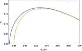
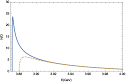
Figure 3: Comparison of the integrand of Eq. (31) for charged and neutral channels without or with the denominators (N or N/D) respectively. The solid line represents the neutral $\bar{D}D^{*}$ channel and the dashed one the charged channel. The left figure shows the contributions of the numerator only and the right figure shows the whole integrand with the denominators.

After the amplitudes are calculated by integrating up to infinity in (31), one could obtain the relative ratio of the transition amplitudes, $\frac{M(X\rightarrow J/\psi\omega)/\sqrt{P_{J/\psi\omega}}}{M(X\rightarrow J/\psi\rho)/\sqrt{P_{J/\psi\rho}}}=3.24\sim 2.43$, with $X(3872)$ mass ranging from 3871.0 MeV to 3871.7 MeV, which is consistent with the expectation of SuzukiSuzuki (2005) to produce a reasonable isospin breaking. In principle, to obtain the decay widths using Eq. (32), the $\rho,\omega$ masses in the scattering amplitudes of $\bar{D}D^{*}\rightarrow J/\psi\rho,\omega$ should be regarded as variables. However, since the numerical calculation of the scattering amplitudes involve six-dimension integration, the integration would be difficult and costs too much computer time. We have checked that the numerical values of the scattering amplitudes changes very slowly when the masses of $\rho,\omega$ changes. Thus, in a practical manner, we did not calculate the integration directly but approximately calculated the scattering amplitudes with the $\rho,\omega$ masses fixed at their central values in PDG and product the phase space kinematic factors. If we cut off the $\pi^{+}\pi^{-}$ invariant mass at $0.45$ GeV and the $\pi^{+}\pi^{-}\pi^{0}$ invariant mass at 0.75 GeV as chosen by Belle and BABAR Abe et al. (2005); del Amo Sanchez et al. (2010), the kinematic space ratio will be

$$\frac{\int_{3m_{\pi}}^{m_{X}-m_{J/\psi}}\frac{|P_{J/\psi\omega}|\Gamma_{\omega}}{(E-m_{\omega})^{2}+\Gamma_{\omega}^{2}/4}\mathrm{d}E}{\int_{2m_{\pi}}^{m_{X}-m_{J/\psi}}\frac{|P_{J/\psi\rho}|\Gamma_{\rho}}{(E-m_{\rho})^{2}+\Gamma_{\rho}^{2}/4}\mathrm{d}E}=0.088\sim 0.098$$ (33)

as the mass of $X(3872)$ ranges from 3871.0 MeV to 3871.7 MeV and the branch fraction will be

$$\frac{\Gamma_{J/\psi\pi^{+}\pi^{-}\pi^{0}}}{\Gamma_{J/\psi\pi^{+}\pi^{-}}}=(3.24\sim 2.43)^{2}\times(0.088\sim 0.098)=0.92\sim 0.58.$$ (34)

This numerical results are consistent with the measured ratio $1.0\pm 0.4\pm 0.3$ by Belle Abe et al. (2005) and $0.8\pm 0.3$ by BABAR del Amo Sanchez et al. (2010). If the lower limits are chosen at $2m_{\pi}$ and $3m_{\pi}$ physical masses respectively, the ratio of kinematic factors will be $0.161\sim 0.169$ and

$$\frac{\Gamma_{J/\psi\pi^{+}\pi^{-}\pi^{0}}}{\Gamma_{J/\psi\pi^{+}\pi^{-}}}=(3.24\sim 2.43)^{2}\times(0.161\sim 0.169)=1.69\sim 0.99.$$ (35)

As a byproduct, this scheme can also provide a qualitative interpretation to the $\bar{D}^{0}D^{0*}$ mass distribution in $B\rightarrow\bar{D}^{0}D^{0*}K$ processes by Belle and BABAR Aubert et al. (2008); Aushev et al. (2010). Since the multi-channel scattering amplitudes could be obtained similar to Eq. (8) as in Ref. Xiao and Zhou (2017), the $T$-matrix of $\bar{D}^{0}D^{0*}$ scatterings could be obtained as

$$T_{SL}(\bar{D}^{0}D^{0*}\rightarrow\bar{D}^{0}D^{0*})=\frac{|f^{\bar{D}^{0}D^{0*}}_{SL}(E)|^{2}}{\eta^{+}(E)}.$$ (36)

If the weak interaction vertex in $B\rightarrow X(\bar{D}^{0}D^{0*})K$ decays is supposed to be a smooth mildly changing factor and could be simulated by a constant, the mass distribution of the $\bar{D}^{0}D^{0*}$ final states is proportional to the $|T(\bar{D}^{0}D^{0*}\rightarrow\bar{D}^{0}D^{0*})|^{2}$ and the phase space factors. A qualitative agreement could be found between the calculations and the experiment data up to a rescaling factor, as shown in Fig. 4. The dotted, solid, and dashed lines in Fig. 4 represent the $X(3872)$ mass at 3.8710, 3.8714, and 3.8717 GeV, respectively, up to a rescaling factor.

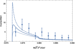
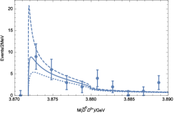
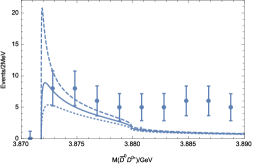
Figure 4: The experimental $\bar{D}^{0}D^{0*}$ mass distributions in $B\rightarrow X(\bar{D}^{0}D^{0*})K$ decays of BABAR (left) Aushev et al. (2010) and Belle (middle and right) Aubert et al. (2008) compared with $r|T(\bar{D}^{0}D^{0*}\rightarrow\bar{D}^{0}D^{0*})|^{2}\cdot phasespace$, where $r$ is a rescaling factor chosen by hand. The dotted, solid, and dashed lines represent the curves with $X(3872)$ mass at 3.8710, 3.8714, and 3.8717 GeV, respectively.

IV Summary

In this paper, we perform a calculation on the branching ratio of $X(3872)$ transition to $J/\psi\pi^{+}\pi^{-}\pi^{0}$ and $J/\psi\pi^{+}\pi^{-}$ based on the Friedrichs-like scheme combined with the quark rearrangement model and QPC model. In our previous work Zhou and Xiao (2017), the first excited $P$-wave charmonium state spectrum is reproduced using the same Friedrichs scheme combined with QPC with GI’s bare spectrum as input, and the results are consistent with the experiment, which demonstrates the reasonability of this scheme. In fact, this scheme provides a general way to incorporate the hadron interactions into the GI quark model. The $X(3872)$ is dynamically generated as a bound state just below the $D^{*0}\bar{D}^{0}$, composed of a dominant $\bar{D}^{0}D^{0*}$ continuum component of about $64\sim 85\%$, a $c\bar{c}$ component of about $10\sim 24\%$, and other continuum. The $X(3872)$ wave function can be explicitly expressed. Based on these information, in present paper we studied the isospin breaking effect within this framework. Since the $X(3872)$ is mostly composed of continuum and the $c\bar{c}$ contribution is also suppressed by OZI rule, we can only consider the continuum contributions to the decay amplitude. In the spirit of the quark rearrangement model, by considering the spin-spin, color Coulomb, and linear potential interactions among the quarks in different mesons, one can obtain the transition amplitudes for $X(3872)$ to $J/\psi\omega$ and $J/\psi\rho$, using the wave function obtained from the Friedrichs-scheme. By taking into account the mass difference of the final states, we obtain the numerical result $\frac{\Gamma_{J/\psi\pi^{+}\pi^{-}\pi^{0}}}{\Gamma_{J/\psi\pi^{+}\pi^{-}}}=0.92\sim 0.58$ as the $X(3872)$ mass changes from 3871.0 MeV to 3871.7 MeV, which is comparable to the experiments. We notice that to provide a reasonable magnitude of the isospin breaking amplitude, the proximity of the $X(3872)$ position to the $D^{0}D^{0*}$ plays an important role. It greatly amplifies the amplitude to $D^{0}\bar{D}^{0*}$ near threshold which causes a large isospin breaking effect in the amplitude as shown in Figure 3. This amplification effect also presents in the integration in the compositeness calculation. Thus, the precise near-threshold behavior of the form factor is important for this result to be solid. Since our calculations are based on GI’s wave functions, which supposedly are the de facto standard in the literature, they presumably provide a more precise form factor which makes our results more solid and convincing.

In this calculation, because the interaction Hamiltonian between the quarks of different meson in the quark rearrangement model is similar to GI’s quark potential model, there is no new parameters introduced in the calculation. All the model parameters except the quark production rate from the vacuum, $\gamma$, are fixed at the well-accepted GI model. The $\gamma$ parameter is also chosen such that the $X(3872)$ is around the experimental mass and all the other observed first excited $P$-wave states are reproduced well as in Zhou and Xiao (2017). One of the merits of using our scheme is that the high energy contribution in the integration in calculating the decay amplitudes is naturally suppressed by the form factor obtained from QPC model based on the wave function from GI’s relativized quark model. Thus, unlike in Suzuki (2005) and Meng and Chao (2007) where the result is cutoff dependent, here no cutoff is introduced and thus the result is more robust.