Quantum Monte Carlo Calculations of Light Nuclei

Abstract

Accurate quantum Monte Carlo calculations of ground and low-lying excited states of light p-shell nuclei are now possible for realistic nuclear Hamiltonians that fit nucleon-nucleon scattering data. At present, results for more than 30 different $(J^{\pi};T)$ states, plus isobaric analogs, in $A\leq 8$ nuclei have been obtained with an excellent reproduction of the experimental energy spectrum. These microscopic calculations show that nuclear structure, including both single-particle and clustering aspects, can be explained starting from elementary two- and three-nucleon interactions. Various density and momentum distributions, electromagnetic form factors, and spectroscopic factors have also been computed, as well as electroweak capture reactions of astrophysical interest.

With permission from the Annual Review of Nuclear and Particle Science. Final version of this material is scheduled to appear in the Annual Review of Nuclear and Particle Science Vol. 51, to be published in December 2001 by Annual Reviews, http://AnnualReviews.org.

1 INTRODUCTION

A major goal of nuclear physics is to understand the stability, structure, and reactions of nuclei as a consequence of the interactions between individual nucleons. This is an extremely challenging many-body problem, exacerbated by the fact that we do not know in detail what the interactions are. Quantum chromodynamics, the fundamental theory for strong interactions, is so difficult to solve in the nonperturbative regime of low-energy nuclear physics that no one is currently able to quantitatively describe the interactions between two nucleons from first principles. However, we do have a tremendous amount of experimental data on nucleon-nucleon ($N\!N$) scattering and we can construct accurate representations of $N\!N$ interactions by means of two-body potentials. These potentials are complicated, depending on the relative positions, spins, isospins, and momenta of the nucleons, which makes the problem of finding accurate quantum-mechanical solutions of many-nucleon bound and scattering states a demanding task. Nevertheless, a variety of precise calculations have been carried out for the three- and four-nucleon systems which reveal an additional complication: two-nucleon forces alone are inadequate to quantitatively explain either the bound-state properties or a variety of $Nd$ and $Nt$ scattering data. This is not surprising, because meson-exchange theory and the composite nature of nucleons indicate that many-nucleon forces, at least three-nucleon forces, are important. However, these are even more difficult to construct from first principles. In like manner, meson-exchange introduces two-body charge and current operators, and calculations of electroweak transitions show that these are also necessary to achieve agreement with data.

Despite these difficulties, tremendous progress has been made in the past decade, both in the characterization of nuclear forces and currents, and in the development of accurate many-body techniques for evaluating them. A multienergy partial-wave analyses of elastic $N\!N$ scattering data below $T_{lab}=350$ MeV was produced by the Nijmegen group in 1993 (?), which demonstrated that over 4300 data points could be fit with a $\chi^{2}$ per datum $\approx$ 1. This was achieved by careful attention to the known long-range part of the $N\!N$ interaction and a rigorous winnowing of inconsistent data. Their work inspired the construction of a number of new $N\!N$ potential models which gave comparably good fits to the database.

Concurrently, several essentially exact methods have been developed for the study of few-nucleon ($A$ = 3,4) systems with such realistic $N\!N$ potentials. The first accurate, converged calculations of three-nucleon ($N\!N\!N$) bound states were obtained by configuration-space Faddeev methods in 1985 (?), while the first accurate ⁴He bound states were obtained by the Green’s function Monte Carlo method in 1987 (?). Other methods of comparable accuracy have been developed since then for both $A$ = 3,4 bound states and for $N\!N\!N$ scattering. A comprehensive review of many aspects of the few-nucleon problem can be found in the article by Carlson and Schiavilla (?). The result of all the progress in the last decade is that we have obtained an excellent understanding of few-nucleon systems, including both structure and reactions, although a few unanswered problems remain.

Until recently, nuclei larger than $A=4$ have been described within the framework of the nuclear shell model or mean-field pictures such as Skyrme models. The classic description of p-shell ($5\leq A\leq 16$) nuclei was developed by Cohen and Kurath in the 1960s (?). In that work, a large number of experimental levels were fit in terms of a relatively small number of two-body matrix elements, but no direct connection was made to the underlying $N\!N$ force. Beginning with the work of Kuo and Brown (?), approximate methods for relating the shell-model matrix elements to the underlying forces were developed and applied to even larger nuclei. However, in most calculations, only the valence nucleons, i.e., the nucleons in the last unfilled shell, are treated as active, while the core is inert. Recently the first ”no-core” shell model calculations, in which all the nucleons are active, have been made in the p-shell with effective interactions that have been derived by a G-matrix procedure from a realistic underlying $N\!N$ force (?). These calculations agree with the other exact methods for the $A=3,4$ nuclei, but fully-converged calculations for larger systems have not yet been obtained.

The present article focuses on recent developments in quantum Monte Carlo methods that are making the light p-shell nuclei accessible at a level of accuracy close to that obtained for the s-shell ($A\leq 4$) nuclei. The quantum Monte Carlo methods include variational Monte Carlo (VMC) and Green’s function Monte Carlo (GFMC) methods. The VMC is an approximate method (?, ?, ?, ?) that is used as a starting point for the more accurate GFMC calculations. Because of its relative simplicity, the VMC has also been used to make first studies of various reactions, such as the nuclear response to electron (?, ?) or pion scattering (?), and for electroweak capture reactions of astrophysical interest (?, ?). The GFMC is exact in the sense that binding energies can be calculated with an accuracy of better than 2%; it has been used to compute ground states and low-lying excitations of all the $A\leq 8$ nuclei (?, ?, ?, ?). These studies of light p-shell nuclei have shown that nuclear structure can be predicted from the elementary nuclear forces. As presently implemented, both the VMC and GFMC methods require significant additional computer resources for every nucleon added, so they probably will be limited to systems of $A\leq 12$ nuclei. A new method, whose accuracy lies between that of the VMC and GFMC methods, is auxiliary-field diffusion Monte Carlo (AFDMC); it has been implemented for large pure neutron systems (?) and with further development should be capable of handling nuclei above $A=12$.

Most of the calculations discussed here have been made using Hamiltonians containing the Argonne $v_{18}$ $N\!N$ potential (?) alone or with one of the Urbana (?) or Illinois (?) series of $N\!N\!N$ potentials. Argonne $v_{18}$ (AV18) is representative of the modern $N\!N$ potentials that give accurate fits to scattering data, while the Urbana and Illinois models are modern $N\!N\!N$ potentials based on meson-exchange interactions and fit to the binding energies of light nuclei. These models are described in some detail in Section 2 to show the complexity of modern nuclear forces, and the consequent challenge for many-body theory. The VMC method is presented in Section 3; it starts with the construction of a variational wave function of specified angular momentum, parity and isospin, $\Psi_{V}(J^{\pi};T)$, using products of two- and three-body correlation operators acting on a fully antisymmetrized set of one-body basis states coupled to specific quantum numbers. Metropolis Monte Carlo integration (?) is used to evaluate $\langle\Psi_{V}|H|\Psi_{V}\rangle$, giving an upper bound to the energy of the state. The GFMC method, described in Section 4, is a stochastic method that systematically improves on $\Psi_{V}$ by projecting out excited state contamination using the Euclidean propagation $\Psi(\tau)=\exp[-(H-E_{0})\tau]\Psi_{V}$. In the limit $\tau\rightarrow\infty$, this leads to the exact $\langle|H|\rangle$.

Energy results for the ground states and many low-lying excited states of the $A\leq 8$ nuclei are presented in Section 5. With the new Hamiltonians, the excitation spectra are reproduced very well, including the relative stability of different nuclei and the splittings between excited states. Energy differences between isobaric analog states and isospin-mixing matrix elements have also been computed to study the charge-independence-breaking of the strong and electromagnetic forces. A variety of density and momentum distributions, electromagnetic moments and form factors, transition densities, spectroscopic factors, and intrinsic deformation are presented in Section 6. One of the chief benefits of this approach is that absolute normalizations can be computed, and effective charges so commonly needed in traditional shell-model calculations of electroweak transitions are not required.

While the quantum Monte Carlo methods have been used primarily for stationary states, it is also possible to study scattering states, as discussed in Section 7. Some first calculations of astrophysical radiative capture reactions in the p-shell are presented in Section 8. Both of these applications are in their early stages, but promise to be major fields of endeavor for future work. In Section 9 we discuss neutron drops, systems of interacting neutrons confined in an artificial external well, that can serve as reference points for the development of Skyrme interactions for use in very large neutron-rich nuclei. Finally, in Section 10, we consider the outlook for future developments.

2 HAMILTONIAN AND CURRENTS

The Hamiltonian used in this review use includes nonrelativistic kinetic energy, the AV18 $N\!N$ potential (?) and either the Urbana IX (?) or one of the new Illinois series of $N\!N\!$ potential (?):

$$H=\sum_{i}K_{i}+\sum_{i<j}v_{ij}+\sum_{i<j<k}V_{ijk}\ .$$ (1)

The kinetic energy operator has charge-independent (CI) and charge-symmetry-breaking (CSB) components, the latter due to the difference between proton and neutron masses,

$$K_{i}=K^{CI}_{i}+K^{CSB}_{i}\equiv-\frac{\hbar^{2}}{4}(\frac{1}{m_{p}}+\frac{1}{m_{n}})\nabla^{2}_{i}-\frac{\hbar^{2}}{4}(\frac{1}{m_{p}}-\frac{1}{m_{n}})\tau_{zi}\nabla^{2}_{i}~{},$$ (2)

where $\mbox{\boldmath$\tau$}_{i}$ is the isospin of nucleon $i$.

The AV18 potential is written as a sum of electromagnetic and one-pion-exchange terms and a shorter-range phenomenological part,

$$v_{ij}=v^{\gamma}_{ij}+v^{\pi}_{ij}+v^{R}_{ij}\ .$$ (3)

The electromagnetic terms include one- and two-photon-exchange Coulomb interaction, vacuum polarization, Darwin-Foldy, and magnetic moment terms, all with appropriate proton and neutron form factors. The one-pion-exchange part of the potential includes the charge-dependent (CD) terms due to the difference in neutral and charged pion masses. It can be written as

$$v^{\pi}_{ij}=f^{2}\left(\frac{m}{m_{s}}\right)^{2}\textstyle{1\over 3}mc^{2}\left[X_{ij}\mbox{\boldmath$\tau$}_{i}\cdot\mbox{\boldmath$\tau$}_{j}+\tilde{X}_{ij}T_{ij}\right]\ ,$$ (4)

where $T_{ij}=3\tau_{zi}\tau_{zj}-\mbox{\boldmath$\tau$}_{i}\cdot\mbox{\boldmath$\tau$}_{j}$ is the isotensor operator and

$$X_{ij}=\textstyle{1\over 3}\left(X^{0}_{ij}+2X^{\pm}_{ij}\right),$$ (5)

$$\tilde{X}_{ij}=\textstyle{1\over 3}\left(X^{0}_{ij}-X^{\pm}_{ij}\right),$$ (6)

$$X^{m}_{ij}=\left[Y(mr_{ij})\mbox{\boldmath$\sigma$}_{i}\cdot\mbox{\boldmath$\sigma$}_{j}+T(mr_{ij})S_{ij}\right]\ .$$ (7)

Here $Y(x)$ and $T(x)$ are the normal Yukawa and tensor functions:

$$Y(x) = \frac{e^{-x}}{x}\ \xi_{Y}(r)\ ,$$ (8)

$$T(x) = \left(\frac{3}{x^{2}}+\frac{3}{x}+1\right)Y(x)\ \xi_{T}(r)\ .$$ (9)

with short-range cutoff functions $\xi_{Y}(r)$ and $\xi_{T}(r)$, and the $X^{\pm,0}$ are calculated with $m=m_{\pi^{\pm}}$ and $m_{\pi^{0}}$. The coupling constant in Eq.(4) is $f^{2}=0.075$ and the scaling mass $m_{s}=m_{\pi^{\pm}}$.

The remaining terms are of intermediate (two-pion-exchange) and short range, with some 40 adjustable parameters. The one-pion-exchange and the remaining phenomenological part of the potential can be written as a sum of eighteen operators,

$$v^{\pi}_{ij}+v^{R}_{ij}=\sum_{p=1,18}v_{p}(r_{ij})O^{p}_{ij}\ .$$ (10)

The first fourteen are CI operators,

$$O^{p=1,14}_{ij}=[1,\mbox{\boldmath$\sigma$}_{i}\cdot\mbox{\boldmath$\sigma$}_{j},S_{ij},{\bf L\cdot S},{\bf L}^{2},{\bf L}^{2}(\mbox{\boldmath$\sigma$}_{i}\cdot\mbox{\boldmath$\sigma$}_{j}),({\bf L\cdot S})^{2}]\otimes[1,\mbox{\boldmath$\tau$}_{i}\cdot\mbox{\boldmath$\tau$}_{j}]~{},$$ (11)

while the last four,

$$O^{p=15,18}_{ij}=[1,\mbox{\boldmath$\sigma$}_{i}\cdot\mbox{\boldmath$\sigma$}_{j},S_{ij}]\otimes T_{ij}\ ,{\rm and}\ (\tau_{zi}+\tau_{zj})\ ,$$ (12)

are CD and CSB terms. The potential was fit directly to the Nijmegen $N\!N$ scattering data base (?) containing 1787 $pp$ and 2514 $np$ data in the range 0–350 MeV, to the $nn$ scattering length, and to the deuteron binding energy, with a $\chi^{2}$ per datum of 1.09.

While the CD and CSB terms are small, there is a clear need for their presence. The Nijmegen group studied many $N\!N$ potentials from the 1980s and before, and found that potentials fit to $np$ data in $T=1$ states did not fit $pp$ data well even after allowing for standard Coulomb effects, and vice versa (?). All five modern $N\!N$ potentials, Reid93, Nijm I and II (?), CD Bonn (?), and AV18, which fit $pp$ and $np$ scattering data with a $\chi^{2}/$point near 1, have CD components. The CSB term is required to fit the difference between the $pp$ and $nn$ scattering lengths, and is consistent with the mass difference between ³H and ³He, as shown below. The identification of the proper CI, CD, and CSB $N\!N$ force components is important in setting the proper baseline for the introduction of $N\!N\!N$ forces, which are required to fit the ³H and ³He binding energies as a primary constraint.

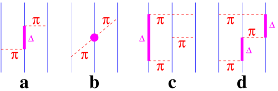
Figure 1: Three-body force Feynman diagrams: a is the Fujita-Miyazawa or two-pion P-wave, b is two-pion S-wave, c and d are three-pion rings with one $\Delta$ in intermediate states.

The Urbana series of three-nucleon potentials is written as a sum of two-pion-exchange P-wave and remaining shorter-range phenomenological terms,

$$V_{ijk}=V^{2\pi,P}_{ijk}+V^{R}_{ijk}~{}.$$ (13)

The structure of the two-pion P-wave exchange term with an intermediate $\Delta$ excitation (Fig. 1a) was originally written down by Fujita and Miyazawa (?); it can be expressed simply as

$$V^{2\pi,P}_{ijk}=\sum_{cyc}\left(A^{P}_{2\pi}\{X^{\pi}_{ij},X^{\pi}_{jk}\}\{\mbox{\boldmath$\tau$}_{i}\cdot\mbox{\boldmath$\tau$}_{j},\mbox{\boldmath$\tau$}_{j}\cdot\mbox{\boldmath$\tau$}_{k}\}+C^{P}_{2\pi}[X^{\pi}_{ij},X^{\pi}_{jk}][\mbox{\boldmath$\tau$}_{i}\cdot\mbox{\boldmath$\tau$}_{j},\mbox{\boldmath$\tau$}_{j}\cdot\mbox{\boldmath$\tau$}_{k}]\right)\ ,$$ (14)

where $X^{\pi}_{ij}$ is constructed with an average pion mass, $m_{\pi}=\textstyle{1\over 3}m_{\pi^{0}}+\textstyle{2\over 3}m_{\pi^{\pm}}$, and $\sum_{cyc}$ is a sum over the three cyclic exchanges of nucleons $i,j,k$. For the Urbana models $C^{P}_{2\pi}=\textstyle{1\over 4}A^{P}_{2\pi}$, as in the original Fujita-Miyazawa model (?), while other potentials like the Tucson-Melbourne (?) and Brazil (?) models, have a ratio slightly larger than $\textstyle{1\over 4}$. The shorter-range phenomenological term is given by

$$V^{R}_{ijk}=\sum_{cyc}A_{R}T^{2}(m_{\pi}r_{ij})T^{2}(m_{\pi}r_{jk})\ .$$ (15)

For the Urbana IX (UIX) model, the parameters were determined by fitting the binding energy of ³H and the density of nuclear matter in conjunction with AV18.

As shown below, while the combined AV18/UIX Hamiltonian reproduces the binding energies of s-shell nuclei, it does not do so well for light p-shell nuclei. Recently a new class of $N\!N\!N$ potentials, called the Illinois models, has been developed to address this problem (?). These potentials contain the Urbana terms and two additional terms, resulting in a total of four coupling constants that can be adjusted to fit the data.

One term, $V^{2\pi,S}_{ijk}$, is due to $\pi N$ S-wave scattering as illustrated in Fig. 1b. It has been included in a number of $N\!N\!N$ potentials like the Tucson-Melbourne (?) and Brazil (?) models. The Illinois models use the form recommended in the latest Texas model (?), where chiral symmetry is used to constrain the structure of the interaction. However, in practice, this term is much smaller than the $V^{2\pi,P}_{ijk}$ contribution and behaves similarly in light nuclei, so it is difficult to establish its strength independently just from calculations of energy levels.

A more important addition is a simplified form for three-pion rings containing one or two deltas (Fig. 1c,d). As discussed in Ref. (?), these diagrams result in a large number of terms, the most important of which are used to construct the Illinois models:

$$V^{3\pi,\Delta R}_{ijk}=A_{3\pi}^{\Delta R}\left[\textstyle{50\over 3}S^{I}_{\tau}S^{I}_{\sigma}+\textstyle{26\over 3}A^{I}_{\tau}A^{I}_{\sigma}\right]\ .$$ (16)

Here the $S^{I}_{x}$ and $A^{I}_{x}$ are operators that are symmetric or antisymmetric under any exchange of the three nucleons, and the subscript $x=\sigma$ or $\tau$ indicates that the operators act on, respectively, spin and space or just isospin degrees of freedom.

The $S^{I}_{\tau}$ is a projector onto isospin-$\textstyle{3\over 2}$ triples:

$$S^{I}_{\tau}=2+\textstyle{2\over 3}\left(\mbox{\boldmath$\tau$}_{i}\cdot\mbox{\boldmath$\tau$}_{j}+\mbox{\boldmath$\tau$}_{j}\cdot\mbox{\boldmath$\tau$}_{k}+\mbox{\boldmath$\tau$}_{k}\cdot\mbox{\boldmath$\tau$}_{i}\right)=4P_{T=3/2}\ .$$ (17)

To the extent isospin is conserved, there are no such triples in the s-shell nuclei, and so this term does not affect them. It is also zero for $Nd$ scattering. However, the $S^{I}_{\tau}S^{I}_{\sigma}$ term is attractive in all the p-shell nuclei studied. The $A^{I}_{\tau}$ has the same structure as the isospin part of anticommutator part of $V^{2\pi,P}$, but the $A^{I}_{\tau}A^{I}_{\sigma}$ term is repulsive in all nuclei studied so far. In p-shell nuclei, the magnitude of the $A^{I}_{\tau}A^{I}_{\sigma}$ term is smaller than that of the $S^{I}_{\tau}S^{I}_{\sigma}$ term, so the net effect of the $V^{3\pi,\Delta R}_{ijk}$ is slight repulsion in s-shell nuclei and larger attraction in p-shell nuclei. The reader is referred to Ref. (?), and its appendix, for the complete structure of $V^{3\pi,\Delta R}_{ijk}$.

Relativistic corrections to the Hamiltonian of Eq.(1) have been studied in three- and four-body nuclei (?, ?, ?). We only briefly outline the results here. If a square-root kinetic energy,

$$K^{rel}_{i}=\sqrt{p^{2}_{i}+m^{2}_{i}}-m_{i}\ ,$$ (18)

where $p_{i}$ is the momentum of nucleon $i$, is introduced into the Hamiltonian, then the $N\!N$ potential must be readjusted to refit the $N\!N$ data. This can be done for AV18 with only small adjustments of the parameters, to produce a $v^{rel}$. VMC calculations show that the resulting $\langle K^{rel}+v^{rel}\rangle\sim\langle K+v\rangle$ for ³H and ⁴He; thus the square-root kinetic energy may be neglected in light nuclei.

A second relativistic correction, the so-called “boost correction,” arises from the fact that the two-nucleon interaction $v_{ij}$ depends both on the relative momentum ${\bf p}=({\bf p}_{i}-{\bf p}_{j})/2$ and the total momentum ${\bf P}={\bf p}_{i}+{\bf p}_{j}$ of the interacting nucleons,

$$v_{ij}({\bf p},{\bf P})=\tilde{v}_{ij}({\bf p})+\delta v_{ij}({\bf p},{\bf P})\ ,$$ (19)

where $\delta v_{ij}({\bf p},{\bf P}=0)=0$. Fitting the two-body potential to two-nucleon scattering data determines only $\tilde{v}_{ij}$. The $\delta v_{ij}$ can be determined from $\tilde{v}_{ij}$; a suitable approximation (?, ?, ?) is

$$\delta{v_{ij}}({\bf P})=-\frac{P^{2}}{8m^{2}}\tilde{v}_{ij}+\frac{1}{8m^{2}}\,\left[\ {\bf P}\cdot{\bf r}\;{\bf P}\cdot\mbox{\boldmath$\nabla$},\tilde{v}_{ij}\ \right]\ ,$$ (20)

where only the first six terms (the static terms) of $\tilde{v}_{ij}$ are retained and the gradient operators do not act on $\tilde{v}_{ij}$. The $\delta v_{ij}$ is meant to be used only in first-order perturbation in a non-relativistic wave function. Its expectation values in light nuclei are nearly proportional to $\langle V^{R}_{ijk}\rangle$ (?), and thus one can consider that part of $A_{R}$, Eq.(15), comes from $\delta v_{ij}$. This proportionality does not, however, extend to nuclear matter or pure neutron systems. There one must use a reduced $A_{R}^{*}$ that does not contain the part ascribable to $\delta v_{ij}$, and explicitly evaluate $\langle\delta v_{ij}\rangle$; doing so results in a softer equation of state for dense matter.

3 VARIATIONAL MONTE CARLO

The variational method can be used to obtain approximate solutions to the many-body Schrödinger equation, $H\Psi=E\Psi$, for a wide range of nuclear systems, including few-body nuclei, light closed-shell nuclei, nuclear matter, and neutron stars (?). A suitably parameterized wave function, $\Psi_{V}$, is used to calculate an upper bound to the exact ground-state energy,

$$E_{V}=\frac{\langle\Psi_{V}|H|\Psi_{V}\rangle}{\langle\Psi_{V}|\Psi_{V}\rangle}\geq E_{0}\ .$$ (21)

The parameters in $\Psi_{V}$ are varied to minimize $E_{V}$, and the lowest value is taken as the approximate solution. Upper bounds to excited states are also obtainable, if they have different quantum numbers from the ground state, or from small-basis diagonalizations if they have the same quantum numbers. The corresponding $\Psi_{V}$ can be used to calculate other properties, such as particle density or electromagnetic moments, or to start a Green’s function Monte Carlo calculation. In this section we describe the ansatz for $\Psi_{V}$ for light nuclei and briefly review how the expectation value is evaluated and the parameters of $\Psi_{V}$ are fixed.

The best variational wave function has the form (?)

$$|\Psi_{V}\rangle=\left[1+\sum_{i<j<k}(U_{ijk}+U^{TNI}_{ijk})+\sum_{i<j}U^{LS}_{ij}\right]|\Psi_{P}\rangle\ ,$$ (22)

where the pair wave function, $\Psi_{P}$, is given by

$$|\Psi_{P}\rangle=\left[{\cal S}\prod_{i<j}(1+U_{ij})\right]|\Psi_{J}\rangle\ .$$ (23)

The $U_{ij}$, $U^{LS}_{ij}$, $U_{ijk}$, and $U^{TNI}_{ijk}$ are noncommuting two- and three-nucleon correlation operators, and ${\cal S}$ is a symmetrization operator. The form of the antisymmetric Jastrow wave function, $\Psi_{J}$, depends on the nuclear state under investigation. For the s-shell nuclei the simple form

$$|\Psi_{J}\rangle=\left[\prod_{i<j<k}f^{c}_{ijk}({\bf r}_{ik},{\bf r}_{jk})\prod_{i<j}f_{c}(r_{ij})\right]|\Phi_{A}(JMTT_{3})\rangle\$$ (24)

is used. Here $f_{c}(r_{ij})$ and $f^{c}_{ijk}$ are central (spin-isospin independent) two- and three-body correlation functions and $\Phi_{A}$ is an antisymmetrized spin-isospin state, e.g.,

$$|\Phi_{3}(\textstyle{1\over 2}\textstyle{1\over 2}\textstyle{1\over 2}\textstyle{1\over 2})\rangle={\cal A}|\uparrow p\downarrow p\uparrow n\rangle\ ,$$ (25)

$$|\Phi_{4}(0000)\rangle={\cal A}|\uparrow p\downarrow p\uparrow n\downarrow n\rangle\ ,$$ (26)

with ${\cal A}$ the antisymmetrization operator.

The two-body correlation operators $U_{ij}$ and $U^{LS}_{ij}$ are sums of spin, isospin, tensor, and spin-orbit terms:

$$U_{ij} = \sum_{p=2,6}\left[\prod_{k\not=i,j}f^{p}_{ijk}({\bf r}_{ik},{\bf r}_{jk})\right]u_{p}(r_{ij})O^{p}_{ij}\ ,$$ (27)

$$U^{LS}_{ij} = \sum_{p=7,8}\left[\prod_{k\not=i,j}f^{p}_{ijk}({\bf r}_{ik},{\bf r}_{jk})\right]u_{p}(r_{ij})O^{p}_{ij}\ ,$$ (28)

where the $O^{p}_{ij}$ were introduced in Eq.(11). The spin-orbit correlations are only summed in Eq.(22) because of the extra computational expense of evaluating powers of ${\bf L\cdot S}$ that would occur if it was inserted in the symmetrized product of Eq.(23).

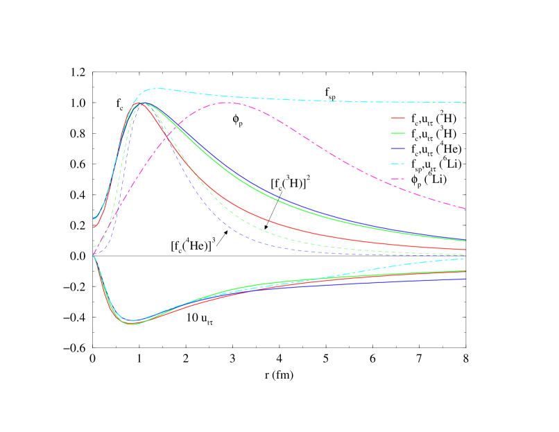
Figure 2: Correlation functions in light nuclei: the central pair correlation, $f_{c}$, and tensor-isospin correlation, $u_{t\tau}$, for s-shell nuclei are shown with solid lines. The dashed lines show $f_{c}^{2}(^{3}$H) and $f_{c}^{3}(^{4}$He) to illustrate the long-range separation behavior. The dot-dashed lines show the central correlation between s- and p-shell nucleons, $f_{sp}$, the $u_{t\tau}$, and the one-body wave function, $\phi^{LS[n]}_{p}$, for ⁶Li.

The central $f_{c}(r)$ and noncentral $u_{p}(r)$ pair correlation functions reflect the influence of the two-body potential at short distances, while satisfying asymptotic boundary conditions of cluster separability. Reasonable functions are generated by minimizing the two-body cluster energy of a somewhat modified $N\!N$ interaction; this results in a set of eight coupled, Schrödinger-like, differential equations corresponding to linear combinations of the first eight operators i of $v_{ij}$, with a number of embedded variational parameters (?). The $f_{c}(r)$ is small at short distances, to reduce the contribution of the repulsive core of $v_{ij}$, and peaks at an intermediate distance corresponding to the maximum attraction of $v_{ij}$, as illustrated in Fig. 2 for several nuclei. For the s-shell nuclei, $f_{c}(r)$ falls off at larger distances to keep the system confined. For example, in ⁴He, $[f_{c}(r)]^{3}\sim{\rm{exp}}(-\kappa r)/r$ at large r, as shown by the dashed line in Fig. 2, where $\kappa$ corresponds to an $\alpha\rightarrow t+p$ separation energy. The noncentral $u_{p}(r)$ are all relatively small; the most important is the long-range tensor-isospin part $u_{t\tau}(r)$, also shown in Fig. 2 for several nuclei, which is mainly induced by the one-pion-exchange part of $v_{ij}$.

The $f^{c}_{ijk}$, $f^{p}_{ijk}$, and $U_{ijk}$ are three-nucleon correlations also induced by $v_{ij}$ (?). The $U^{TNI}_{ijk}$ are three-body correlations induced by the three-nucleon interaction, which have the form suggested by perturbation theory:

$$U^{TNI}_{ijk}=\sum_{x}\epsilon_{x}V_{ijk}(\tilde{r}_{ij},\tilde{r}_{jk},\tilde{r}_{ki})\ ,$$ (29)

with $\tilde{r}=yr$, $y$ a scaling parameter, and $\epsilon_{x}$ a (small negative) strength parameter. A somewhat simpler wave function to evaluate than $\Psi_{V}$ is given by:

$$|\Psi_{T}\rangle=\left[1+\sum_{i<j<k}\tilde{U}^{TNI}_{ijk}\right]|\Psi_{P}\rangle\ ,$$ (30)

where $\tilde{U}^{TNI}_{ijk}$ is a slightly truncated TNI correlation. The $\Psi_{T}$ gives about $1-2$ MeV less binding than the full $\Psi_{V}$, but costs less than half as much to construct, making it a more efficient starting point for the GFMC calculation (?).

The Jastrow wave function for the light p-shell nuclei is more complicated, as a number of nucleons must be placed in the unfilled p-shell. The $LS$ coupling scheme is used to obtain the desired $JM$ value of a given state, as suggested by the shell-model studies of light p-shell nuclei (?). Different possible $LS$ combinations lead to multiple components in the Jastrow wave function. The possibility that the central correlations $f_{c}(r_{ij})$ could depend upon the shells (s or p) occupied by the particles and on the $LS$ coupling is also allowed for:

$$|\Psi_{J}\rangle = {\cal A}\left\{\prod_{i<j<k}f^{c}_{ijk}\prod_{i<j\leq 4}f_{ss}(r_{ij})\prod_{k\leq 4<l\leq A}f_{sp}(r_{kl})\right.$$

$$\left.\sum_{LS[n]}\Big{(}\beta_{LS[n]}\prod_{4<l<m\leq A}f^{LS[n]}_{pp}(r_{lm})|\Phi_{A}(LS[n]JMTT_{3})_{1234:56\ldots A}\rangle\Big{)}\right\}\ .$$

The operator ${\cal A}$ indicates an antisymmetric sum over all possible partitions of the $A$ particles into 4 s-shell and $(A-4)$ p-shell ones. The central correlation $f_{ss}(r)$ is the $f_{c}(r)$ from the ⁴He wave function. The $f_{sp}(r)$, shown in Fig. 2 for Li nuclei, is similar to the $f_{c}(r)$ at short range, but with a long-range tail going to unity; this helps the wave function factorize to a cluster structure like $\alpha+d$ in ⁶Li or $\alpha+t$ in ⁷Li at large cluster separations. The $f^{LS[n]}_{pp}(r)$ is similar to the deuteron (triton) $f_{c}(r)$ in the case of ⁶Li (⁷Li).

The $LS$ components of the single-particle wave function are given by:

$$|\Phi_{A}(LS[n]JMTT_{3})_{1234:56\ldots A}\rangle=|\Phi_{\alpha}(0000)_{1234}\rangle\prod_{4<l\leq A}\phi^{LS[n]}_{p}(R_{\alpha l})$$ (32)

$$\left\{[\prod_{4<l\leq A}Y_{1m_{l}}(\Omega_{\alpha l})]_{LM_{L}[n]}\times[\prod_{4<l\leq A}\chi_{l}(\textstyle{1\over 2}m_{s})]_{SM_{S}}\right\}_{JM}\times[\prod_{4<l\leq A}\nu_{l}(\textstyle{1\over 2}t_{3})]_{TT_{3}}\rangle\ .$$

The $\phi^{LS[n]}_{p}(R_{\alpha k})$ are p-wave solutions of a particle in an effective $\alpha+N$ potential and are functions of the distance between the center of mass of the $\alpha$ core and nucleon $k$; they may be different for different $LS[n]$ components. A Woods-Saxon potential well,

$$V_{\alpha N}(r)=V^{LS}_{p}[1+exp(\frac{r-R_{p}}{a_{p}})]^{-1}\ ,$$ (33)

where $V^{LS}_{p}$, $R_{p}$, and $a_{p}$ are variational parameters, and a Coulomb term if appropriate is used.

For $A\geq 7$ nuclei, with three or more p-shell particles there are multiple ways of coupling the orbital angular momentum, $L$, spin, $S$, and isospin, $T$, to obtain the total $(J^{\pi};T)$ of the system. The spatial permutation symmetry, denoted by the Young pattern $[n]$, is used to enumerate the different possible terms, as discussed in Appendix 1C of Ref. (?). The different possible contributions to $A$ = 6–8 nuclei are given in Table 1, with the corresponding spin states of highest spatial symmetry for each nucleus.

Table 1: Permutation symmetry terms for $LS$-coupling in $A=6-8$ nuclei and corresponding spin states.

$A$	$[n]$	$L$	$(T,S)$	highest symmetry states
$6$	$[2]$	$0,2$	$(1,0)(0,1)$	6He$(0^{+},2^{+})$, 6Li$(1^{+},2^{+},3^{+})$
	$[11]$	$1$	$(1,1)(0,0)$	6He$(1^{+})$
$7$	$[3]$	$1,3$	$(\textstyle{1\over 2},\textstyle{1\over 2})$	7Li$(\textstyle{1\over 2}^{-},\textstyle{3\over 2}^{-},\textstyle{5\over 2}^{-},\textstyle{7\over 2}^{-})$
	$[21]$	$1,2$	$(\textstyle{3\over 2},\textstyle{1\over 2})(\textstyle{1\over 2},\textstyle{3\over 2})(\textstyle{1\over 2},\textstyle{1\over 2})$	7He$(\textstyle{1\over 2}^{-},\textstyle{3\over 2}^{-},\textstyle{5\over 2}^{-})$
	$[111]$	$0$	$(\textstyle{3\over 2},\textstyle{3\over 2})(\textstyle{1\over 2},\textstyle{1\over 2})$
$8$	$[4]$	$0,2,4$	$(0,0)$	8Be$(0^{+},2^{+},4^{+})$
	$[31]$	$1,2,3$	$(1,1)(1,0)(0,1)$	8Li$(0^{+}-4^{+})$, 8Be$(1^{+},3^{+})$
	$[22]$	$0,2$	$(2,0)(1,1)(0,2)(0,0)$	8He$(0^{+},2^{+})$
	$[211]$	$1$	$(2,1)(1,2)(1,1)(1,0)(0,1)$	8He$(1^{+})$

After other parameters in the trial function have been optimized, a series of calculations are made in which the $\beta_{LS[n]}$ of Eq.(3) may be different in the left- and right-hand-side wave functions to obtain the diagonal and off-diagonal matrix elements of the Hamiltonian and the corresponding normalizations and overlaps. The resulting N$\times$N matrices are diagonalized to find the $\beta_{LS[n]}$ eigenvectors, using generalized eigenvalue routines because the correlated $\Psi_{V}$ are not orthogonal. This allows us to project out not only the ground states, but excited states of the same $(J^{\pi};T)$ quantum numbers. For example, the ground states of ⁶Li, ⁷Li, and ⁸Li are obtained from 3$\times$3, 5$\times$5, and 7$\times$7 diagonalizations, respectively.

The energy expectation value of Eq.(21) is evaluated using Monte Carlo integration. A detailed technical description of the methods used can be found in Refs. (?, ?). Monte Carlo sampling is done both in configuration space and in the order of operators in the symmetrized product of Eq.(23) by following a Metropolis random walk. The expectation value for an operator $O$ is computed with the expression

$$\langle O\rangle=\frac{\sum_{p,q}\int d{\bf R}\left[\Psi_{p}^{\dagger}({\bf R})O\Psi_{q}({\bf R})/W_{pq}({\bf R})\right]W_{pq}({\bf R})}{\sum_{p,q}\int d{\bf R}\left[\Psi_{p}^{\dagger}({\bf R})\Psi_{q}({\bf R})/W_{pq}({\bf R})\right]W_{pq}({\bf R})}\ ,$$ (34)

where samples are drawn from a probability distribution, $W_{pq}({\bf R})$. The subscripts $p$ and $q$ specify the order of operators in the left- and right-hand-side wave functions, while the integration runs over the particle coordinates ${\bf R}=({\bf r}_{1},{\bf r}_{2},\ldots,{\bf r}_{A})$. The probability distribution is constructed from the $\Psi_{P}$ of Eq.(23):

$$W_{pq}({\bf R})=|{\rm Re}(\langle\Psi_{P,p}^{\dagger}({\bf R})\Psi_{P,q}({\bf R})\rangle)|\ .$$ (35)

This is much less expensive to compute than using the full wave function of Eq.(22) with its spin-orbit and operator-dependent three-body correlations, but it typically has a norm within 1–2% of the full wave function.

Expectation values have a statistical error which can be estimated by the standard deviation $\sigma$:

$$\sigma=\left[\frac{\langle O^{2}\rangle-\langle O\rangle^{2}}{N-1}\right]^{1/2}\ ,$$ (36)

where $N$ is the number of statistically independent samples. Block averaging schemes can also be used to estimate the autocorrelation times and determine the statistical error.

The wave function $\Psi$ can be represented by an array of $2^{A}\times(^{A}_{Z})$ complex numbers,

$$\Psi({\bf R})=\sum_{\alpha}\psi_{\alpha}({\bf R})|\alpha\rangle\ ,$$ (37)

where the $\psi_{\alpha}({\bf R})$ are the complex coefficients of each state $|\alpha\rangle$ with specific third components of spin and isospin. This gives vectors with 96, 1280, 4480, and 14336 complex numbers for ⁴He, ⁶Li, ⁷Li, and ⁸Li, respectively. The spin, isospin, and tensor operators $O^{p=2,6}_{ij}$ contained in the two-body correlation operator $U_{ij}$, and in the Hamiltonian are sparse matrices in this basis. For forces that are largely charge-independent, as is the case here, this charge-conserving basis can be replaced with an isospin-conserving basis that has $N(A,T)=2^{A}\times I(A,T)$ components, where

$$I(A,T)=\frac{2T+1}{\textstyle{1\over 2}A+T+1}\left(\begin{array}[]{c}A\\ \textstyle{1\over 2}A+T\end{array}\right)\ .$$ (38)

This reduces the number of vector elements to 32, 320, 1792, and 7168 for the cases given above — a significant savings. In practice, isospin operators are more expensive to evaluate in this basis, but the overall savings in computation is still large. Furthermore, if for even-$A$ nuclei the $M=0$ state is computed, only half the spin components need to be evaluated; the other ones can be found by time-reversal invariance.

Expectation values of the kinetic energy and spin-orbit potential require the computation of first derivatives and diagonal second derivatives of the wave function. These are obtained by evaluating the wave function at $6A$ slightly shifted positions of the coordinates ${\bf R}$ and taking finite differences, as discussed in Ref. (?). Potential terms quadratic in L require mixed second derivatives, which can be obtained by additional wave function evaluations and finite differences.

The rapid growth in the size of $\Psi$ as $A$ increases is the chief limitation, both in computer time and memory requirements, on extending the current method to larger nuclei. The cost of an energy calculation for a given configuration also increases as the number of pairs, $P=\textstyle{1\over 2}A(A-1)$, because of the number of pair operations required to construct $\Psi$, and roughly as the number of particles, $A$, due to the number of wave function evaluations required to compute the kinetic energy by finite differences. These factors are shown in Table 2 for a number of nuclei, with a final overall product showing the cost relative to that for an ⁸Be calculation. Some initial $A=9,10$ calculations have been made, but are at the limit of current computer resources, so while ¹²C should be reached in a few years, it may be the practical limit for this approach. Calculations of nuclei like ¹⁶O or ⁴⁰Ca, will require other methods such as auxiliary-field diffusion Monte Carlo, which samples the spin and isospin components of the wave function by introducing auxiliary fields, as the plain Monte Carlo samples the spatial part. Also shown in the table is the cost for several pure neutron problems, such as an eight-body drop (with external confining potential) or 14 or 38 neutrons in a box (with periodic boundary conditions) as neutron matter simulations. The ⁸n drop has been calculated (?, ?) by VMC and GFMC, and initial box simulations have been done for 14 neutrons by GFMC (?) and up to 54 neutrons by AFDMC (?).

Table 2: Approximate scaling of VMC and GFMC calculations with system size. The number of pairs is $P$, the state-vector size is the product of the number of spin states and number of isospin states, $I(A,T)$; as is discussed in the text, these numbers may be halved for even-$A$ nuclei. The last column is the relative difficulty scaled to ⁸Be, assuming $M=0$ states are computed for even-$A$ nuclei.

	$A$	$P$	$2^{A}\times I(A,T)$	$\prod/\prod(^{8}$Be)
3H	3	3	8$\times$2	0.0004
4He	4	6	16$\times$2	0.001
5He	5	10	32$\times$5	0.020
6Li	6	15	64$\times$5	0.036
7Li	7	21	128$\times$14	0.66
8Be	8	28	256$\times$14	1.
9Be	9	36	512$\times$42	17.
10B	10	45	1024$\times$42	24.
12C	12	66	4096$\times$132	530.
16O	16	120	65536$\times$1430	$2\times 10^{5}$
40Ca	40	780	7$\times 10^{21}$	$3\times 10^{20}$
8n	8	28	256$\times$1	0.071
14n	14	91	16384$\times$1	26.
38n	38	703	3$\times 10^{11}$	$9\times 10^{9}$

A major problem arises in minimizing the variational energy for p-shell nuclei using the above wave functions: there is no variational minimum that gives reasonable rms radii. For example, the variational energy for ⁶Li is slightly more bound than for ⁴He, but is not more bound than for separated ⁴He and ²H nuclei, so the wave function is not stable against breakup into $\alpha+d$ subclusters. Consequently, the energy can be lowered toward the sum of ⁴He and ²H energies by making the wave function more and more diffuse. Such a diffuse wave function would not be useful for computing other nuclear properties, or as a starting point for the GFMC calculation, so the search for variational parameters is constrained by requiring the resulting point proton rms radius, $r_{p}$, to be close to the experimental values for ⁶Li and ⁷Li ground states. For other $A$ = 6–8 ground states, and all the excited states, the trial functions contain minimal changes to the ⁶Li and ⁷Li wave functions, with the added requirement that excited states should not have smaller radii than the ground states. The final step is always the diagonalization of the Hamiltonian in the $\beta_{LS[n]}$ mixing parameters.

4 GREEN’S FUNCTION MONTE CARLO

The GFMC method (?, ?) projects out the exact lowest-energy state, $\Psi_{0}$, for a given set of quantum numbers, using $\Psi_{0}=\lim_{\tau\rightarrow\infty}\exp[-(H-E_{0})\tau]\Psi_{T}$, where $\Psi_{T}$ is an initial trial function. If the maximum $\tau$ actually used is large enough, the eigenvalue $E_{0}$ is calculated exactly while other expectation values are generally calculated neglecting terms of order $|\Psi_{0}-\Psi_{T}|^{2}$ and higher (?). In contrast, the error in the variational energy, $E_{V}$, is of order $|\Psi_{0}-\Psi_{T}|^{2}$, and other expectation values calculated with $\Psi_{T}$ have errors of order $|\Psi_{0}-\Psi_{T}|$. In the following we present a brief overview of modern nuclear GFMC methods; much more detail may be found in Refs. (?, ?).

We start with the $\Psi_{T}$ of Eq.(30) and define the propagated wave function $\Psi(\tau)$

$$\Psi(\tau)=e^{-({H}-E_{0})\tau}\Psi_{T}=\left[e^{-({H}-E_{0})\triangle\tau}\right]^{n}\Psi_{T}\ ,$$ (39)

where we have introduced a small time step, $\tau=n\triangle\tau$; obviously $\Psi(\tau=0)=\Psi_{T}$ and $\Psi(\tau\rightarrow\infty)=\Psi_{0}$. The $\Psi(\tau)$ is represented by a vector function of $\bf R$ using Eq.(37), and the Green’s function, $G_{\alpha\beta}({\bf R},{\bf R}^{\prime})$ is a matrix function of $\bf R$ and ${\bf R}^{\prime}$ in spin-isospin space, defined as

$$G_{\alpha\beta}({\bf R},{\bf R}^{\prime})=\langle{\bf R},\alpha|e^{-({H}-E_{0})\triangle\tau}|{\bf R}^{\prime},\beta\rangle\ .$$ (40)

It is calculated with leading errors of order $(\triangle\tau)^{3}$. Omitting the spin-isospin indices $\alpha$, $\beta$ for brevity, $\Psi({\bf R}_{n},\tau)$ is given by

$$\Psi({\bf R}_{n},\tau)=\int G({\bf R}_{n},{\bf R}_{n-1})\cdots G({\bf R}_{1},{\bf R}_{0})\Psi_{T}({\bf R}_{0})d{\bf R}_{n-1}\cdots d{\bf R}_{1}d{\bf R}_{0}\ ,$$ (41)

with the integral being evaluated stochastically.

The short-time propagator should allow as large a time step $\triangle\tau$ as possible, because the total computational time for propagation is proportional to $1/\triangle\tau$. Earlier calculations (?, ?, ?) used the propagator obtained from the Feynman formulae in which the kinetic and potential energy terms of $H$ are separately exponentiated. The main error in this approximation to $G_{\alpha,\beta}$ comes from terms in $e^{-{H}\triangle\tau}$ having multiple $v_{ij}$, like $v_{ij}Kv_{ij}(\triangle\tau)^{3}$, where $K$ is the kinetic energy, which can become large when particles $i$ and $j$ are very close due to the large repulsive core in $v_{ij}$. This requires a rather small $\triangle\tau\sim 0.1$ GeV^-1.

It has been found in studies of bulk helium atoms (?) that including the exact two-body propagator allows much larger time steps. This short-time propagator is

$$G_{\alpha\beta}({\bf R},{\bf R}^{\prime}) = G_{0}({\bf R},{\bf R}^{\prime})\langle\alpha|\left[{\cal S}\prod_{i<j}\frac{g_{ij}({\bf r}_{ij},{\bf r}_{ij}^{\prime})}{g_{0,ij}({\bf r}_{ij},{\bf r}_{ij}^{\prime})}\right]|\beta\rangle\ ,$$ (42)

where

$$G_{0}({\bf R},{\bf R}^{\prime}) = \langle{\bf R}|e^{-{K}\triangle\tau}|{\bf R}^{\prime}\rangle=\left[\sqrt{\frac{m}{2\pi\hbar^{2}\triangle\tau}}\,\right]^{3A}\exp\left[\frac{-({\bf R}-{\bf R}^{\prime})^{2}}{2\hbar^{2}\triangle\tau/m}\right]\ ,$$ (43)

$g_{ij}$ is the exact two-body propagator,

$$g_{ij}({\bf r}_{ij},{\bf r}_{ij}^{\prime})=\langle{\bf r}_{ij}|e^{-H_{ij}\triangle\tau}|{\bf r}_{ij}^{\prime}\rangle\ ,$$ (44)

and $g_{0,ij}$ is the free two-body propagator. All terms containing any number of the same $v_{ij}$ and $K$ are treated exactly in this propagator, as we have included the imaginary-time equivalent of the full two-body scattering amplitude. It still has errors of order $(\triangle\tau)^{3}$, however they are from commutators of terms like $v_{ij}Kv_{ik}(\triangle\tau)^{3}$ which become large only when both pairs $ij$ and $ik$ are close. Because this is a rare occurrence, a five times larger time step, $\triangle\tau\sim 0.5$ GeV^-1, can be used (?).

Including the three-body forces and the $E_{0}$ in Eq.(40), the complete propagator is given by

$$G_{\alpha\beta}({\bf R},{\bf R}^{\prime}) = e^{E_{o}\triangle\tau}G_{0}({\bf R},{\bf R}^{\prime})\exp[{-\sum(V^{R}_{ijk}({\bf R})+V^{R}_{ijk}({\bf R^{\prime}}))\frac{\triangle\tau}{2}}]$$ (45)

$$\langle\alpha|I_{3}({\bf R})|\gamma\rangle\langle\gamma|\left[{\cal S}\prod_{i<j}\frac{g_{ij}({\bf r}_{ij},{\bf r}_{ij}^{\prime})}{g_{0,ij}({\bf r}_{ij},{\bf r}_{ij}^{\prime})}\right]|\delta\rangle\langle\delta|I_{3}({\bf R}^{\prime})|\beta\rangle~{},$$

where

$$I_{3}({\bf R})=\left[1-\frac{\triangle\tau}{2}\sum V^{\pi}_{ijk}({\bf R})\right]~{}.$$ (46)

and $V^{\pi}_{ijk}=V^{2\pi}_{ijk}+V^{3\pi}_{ijk}$ represents, in general, all non-central $V_{ijk}$ terms. With the exponential of $V^{\pi}_{ijk}$ expanded to first order in $\triangle\tau$, there are additional error terms of the form $V^{\pi}_{ijk}V^{\pi}_{i^{\prime}j^{\prime}k^{\prime}}(\triangle\tau)^{2}$. However, they have negligible effect because $V^{\pi}_{ijk}$ has a magnitude of only a few MeV.

Quantities of interest are evaluated in terms of a “mixed” expectation value between $\Psi_{T}$ and $\Psi(\tau)$:

$$\langle O\rangle_{\rm Mixed} = \frac{\langle\Psi_{T}|O|\Psi(\tau)\rangle}{\langle\Psi_{T}|\Psi(\tau)\rangle}$$ (47)

$$= \frac{\int d{\bf P}_{n}\Psi_{T}^{\dagger}({\bf R}_{n})OG({\bf R}_{n},{\bf R}_{n-1})\cdots G({\bf R}_{1},{\bf R}_{0})\Psi_{T}({\bf R}_{0})}{\int d{\bf P}_{n}\Psi_{T}^{\dagger}({\bf R}_{n})G({\bf R}_{n},{\bf R}_{n-1})\cdots G({\bf R}_{1},{\bf R}_{0})\Psi_{T}({\bf R}_{0})}~{},$$

where ${\bf P}_{n}={\bf R}_{0},{\bf R}_{1},\cdots,{\bf R}_{n}$ denotes the ‘path’, and $d{\bf P}_{n}=d{\bf R}_{0}d{\bf R}_{1}\cdots d{\bf R}_{n}$ with the integral over the paths being carried out stochastically. The desired expectation values would, of course, have $\Psi(\tau)$ on both sides; by writing $\Psi(\tau)=\Psi_{T}+\delta\Psi(\tau)$ and neglecting terms of order $[\delta\Psi(\tau)]^{2}$, we obtain the approximate expression

$$\langle O(\tau)\rangle=\frac{\langle\Psi(\tau)|O|\Psi(\tau)\rangle}{\langle\Psi(\tau)|\Psi(\tau)\rangle}\approx\langle O(\tau)\rangle_{\rm Mixed}+[\langle O(\tau)\rangle_{\rm Mixed}-\langle O\rangle_{T}]~{},$$ (48)

where $\langle O\rangle_{T}$ is the variational expectation value. More accurate evaluations of $\langle O(\tau)\rangle$ are possible (?), essentially by measuring the observable at the mid-point of the path. However, such estimates require a propagation twice as long as the mixed estimate and require separate propagations for every $\langle O\rangle$ to be evaluated. The nuclear calculations published to date use the approximation of Eq.(48).

A special case is the expectation value of the Hamiltonian. The $\langle{H}(\tau)\rangle_{\rm Mixed}$ can be re-expressed as (?)

$$\langle{H}(\tau)\rangle_{\rm Mixed}=\frac{\langle\Psi_{T}|e^{-({H}-E_{0})\tau/2}{H}e^{-({H}-E_{0})\tau/2}|\Psi_{T}\rangle}{\langle\Psi_{T}|e^{-({H}-E_{0})\tau/2}e^{-({H}-E_{0})\tau/2}|\Psi_{T}\rangle}\geq E_{0}~{},$$ (49)

since the propagator $\exp[-(H-E_{0})\tau]$ commutes with the Hamiltonian. Thus $\langle{H}(\tau)\rangle_{\rm Mixed}$ approaches $E_{0}$ in the limit $\tau\rightarrow\infty$, and the expectation value obeys the variational principle for all $\tau$.

The AV18 interaction contains terms that are quadratic in orbital angular momentum, $L$. These terms are, in essence, state- and position-dependent modifications of the mass of the nucleons. If they are included in the calculation of $g_{ij}$, then the ratio $g_{ij}/g_{0,ij}$ in Eq.(43) becomes unbounded for large $|{\bf r}_{ij}|$ or $|{\bf r}_{ij}^{\prime}|$ and the Monte Carlo statistical error will also be unbounded. Hence the GFMC propagator is constructed with a simpler isoscalar interaction, $H^{\prime}$, with a $v^{\prime}_{ij}$ that has only eight operator terms, $[1,\mbox{\boldmath$\sigma$}_{i}\cdot\mbox{\boldmath$\sigma$}_{j},S_{ij},{\bf L\cdot S}]\otimes[1,\mbox{\boldmath$\tau$}_{i}\cdot\mbox{\boldmath$\tau$}_{j}]$, chosen such that it equals the CI part of the full interaction in all S- and P-waves and in the deuteron. The $v^{\prime}_{ij}$ is a little more attractive than $v_{ij}$, so a $V^{\prime}_{ijk}$ adjusted so that $\langle H^{\prime}\rangle\approx\langle H\rangle$ is also used. This ensures the GFMC algorithm will not propagate to excessively large densities due to overbinding. Consequently, the upper bound property applies to $\langle{H}^{\prime}(\tau)\rangle$, and $\langle H-H^{\prime}\rangle$ must be evaluated perturbatively.

Another complication that arises in the GFMC algorithm is the “fermion sign problem”. This arises from the stochastic evaluation of the matrix elements in Eq.(47). The $G({\bf R}_{i},{\bf R}_{i-1})$ is a local operator and can mix in the boson solution. This has a (much) lower energy than the fermion solution and thus is exponentially amplified in subsequent propagations. In the final integration with the antisymmetric $\Psi_{T}$, the desired fermionic part is projected out, but in the presence of large statistical errors that grow exponentially with $\tau$. Because the number of pairs that can be exchanged grows with $A$, the sign problem also grows exponentially with increasing $A$. For $A{\geq}8$, the errors grow so fast that convergence in $\tau$ cannot be achieved.

For simple scalar wave functions, the fermion sign problem can be controlled by not allowing the propagation to move across a node of the wave function. Such “fixed-node” GFMC provides an approximate solution which is the best possible variational wave function with the same nodal structure as $\Psi_{T}$. However, a more complicated solution is necessary for the spin- and isospin-dependent wave functions of nuclei. In the last few years a suitable “constrained path” approximation has been developed and extensively tested, first for condensed matter systems (?) and more recently for nuclei (?). The basic idea of the constrained-path method is to discard those configurations that, in future generations, will contribute only noise to expectation values. If the exact ground state $|\Psi_{0}\rangle$ were known, any configuration for which

$$\Psi({\bf P}_{n})^{\dagger}\Psi_{0}({\bf R}_{n})=0\ ,$$ (50)

where a sum over spin-isospin states is implied, could be discarded. Here ${\bf P}_{n}$ designates the complete path, $({\bf R}_{0},...,{\bf R}_{n})$ that has led to ${\bf R}_{n}$. The sum of these discarded configurations can be written as a state $|\Psi_{d}\rangle$, which obviously has zero overlap with the ground state. The $\Psi_{d}$ contains only excited states and should decay away as $\tau\rightarrow\infty$, thus discarding it is justified. Of course the exact $\Psi_{0}$ is not known, and so configurations are discarded with a probability such that the average overlap with the trial wave function,

$$\langle\Psi_{d}|\Psi_{T}\rangle=0\ .$$ (51)

Many tests of this procedure have been made (?) and it usually gives results that are consistent with unconstrained propagation, within statistical errors. However a few cases in which the constrained propagation converges to the wrong energy (either above or below the correct energy) have been found. Therefore a small number, $n_{u}=10$ to 20, unconstrained steps are made before evaluating expectation values. These few unconstrained steps, out of typically 400 total steps, appear to be enough to damp out errors introduced by the constraint, but do not greatly increase the statistical error.

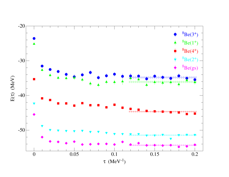
Figure 3: GFMC $E(\tau)$ using AV18/UIX for various states of ⁸Be. Averages with their standard errors are shown by the solid and dashed lines.

Figure 3 shows the progress with increasing $\tau$ of typical constrained GFMC calculations, in this case for various states of ⁸Be. The values shown at $\tau=0$ are the VMC values using $\Psi_{T}$; VMC values with the best known $\Psi_{V}$ are about 1.5 MeV below these. The GFMC very rapidly makes a large improvement on these energies; by $\tau=0.01$ MeV^-1, the $\Psi_{T}$ energies have been reduced by 6.5 to 8 MeV. This rapid improvement corresponds to the removal of small admixtures of states with excitation energies $\sim~{}1$ GeV from $\Psi_{T}$. Averages over typically the last nine $\tau$ values are used as the GFMC energy. The standard deviation, computed using block averaging, of all of the individual energies for these $\tau$ values is used to compute the corresponding statistical error. The solid lines show these averages; the corresponding dashed lines show the statistical errors. The g.s., $1^{+}$, and $3^{+}$ states of ⁸Be have widths less than 250 keV and their $E(\tau)$ appear to be converged and constant over the averaging regime. The $2^{+}$ state has a width of 1.5 MeV and the $4^{+}$ state’s width is 3.5 MeV; the $E(\tau)$ for the $2^{+}$ state might be converged, but that of the $4^{+}$ state is clearly steadily decreasing. Reliable estimates of the energies of broad resonances requires the use of scattering-state boundary conditions (see Sec. 7) which have not yet been implemented for more than five nucleons.

Tests with different $\Psi_{T}$ as starting points for the GFMC calculation are described in Ref. (?). The most crucial aspect in choosing $\Psi_{T}$ is that it have the correct mix of spatial symmetries, i.e., the $\beta_{LS[n]}$ admixtures. This is because the limited propagation time is not sufficient for the GFMC algorithm to filter out low-lying excitations with the same quantum numbers. This issue is unimportant in ⁴He, where the first 0⁺ excited state is near 20 MeV, but in ⁶Li, the first 1⁺ excited state is at only 5.65 MeV; other $p$-shell nuclei have similar low-lying excitations. Otherwise, the GFMC algorithm is able to rapidly correct for some very poor $\Psi_{T}$ whose variational energies are actually positive. However, a good $\Psi_{T}$ helps to keep the error bars small at larger $\tau$. The most efficient balance between speed of construction of $\Psi_{T}$ and smallest number of samples needed to achieve a given error bar seems to be given by Eq.(30). A number of other tests of the GFMC algorithm and its ability to determine nuclear radii are described in Refs. (?, ?).

The calculations described here are computationally intense, and would not have been possible without the advent of parallel supercomputers. The initial studies (?) of ⁶Li required $\sim 2,000$ node hours on an IBM SP1 to propagate 10,000 configurations to $\tau$ = 0.06 MeV^-1. Today, with improvements in the algorithm and after much effort to optimize the computer codes, the same calculation requires about 15 node hours on a third generation IBM SP. However, a present calculation for ⁸Li, requiring 10,000 configurations to get a reasonable error bar, takes 1,000 node hours, so forefront computer resources remain essential for this program.

5 ENERGY RESULTS

There are a number of accurate many-body methods for evaluating the binding energy of the s-shell nuclei, ³H, ³He, and ⁴He, using realistic nuclear forces. These include Faddeev in configuration space (?) (FadR), Faddeev and Faddeev-Yakubovsky in momentum space (?) (FadQ), and hyperspherical harmonics (?) (HH), correlated hyperspherical harmonics (?) (CHH) and pair-correlated hyperspherical harmonics (?) (PHH). Some results of these methods for the AV18 and AV18/UIX Hamiltonians are shown in Table 3. We observe that the VMC upper bounds are generally 1.5–2.0% above the GFMC energies, which in turn are 0.25–1.0% above the Faddeev results. The disagreement between GFMC and the other methods may be attributable to the fact that GFMC is propagated with an $H^{\prime}$ and a small piece of the Hamiltonian is computed in perturbation. At this fine level of comparison, one needs to worry about how features such as $T=\textstyle{3\over 2}$ admixtures and $n-p$ mass differences in the trinucleon ground state are treated in each calculation.

Table 3 also shows the necessity of including (at least) a three-nucleon potential in the Hamiltonian in order to reproduce the A=3,4 experimental binding energies. This is true for all the other modern $N\!N$ potentials, as shown in Refs. (?, ?). The local potentials AV18, Reid93, and Nijm II, give very similar results, while the slightly nonlocal Nijm I gives 1–3% more binding, and the more nonlocal CD-Bonn gives 5–8% more binding, or about halfway between the local potential values and experiment. At present, no two- plus three-nucleon potential combination gives an exact fit to both trinucleon and ⁴He energies, but several combinations, like AV18/UIX, come quite close. It also appears that it may be easier to fit ³He and ⁴He simultaneously, rather than ³H and ⁴He, perhaps because of the better data constraints on the $pp$ interaction compared to the $nn$ interaction (?). In principle, there should also be four-body forces, but their contribution must be quite small, and it is impossible to unambiguously identify a need for such terms until a more thorough survey of possible three-nucleon potentials is made and the discrepancies between the various many-body methods are resolved.

Table 3: Energies of ³H and ⁴He in MeV, computed by VMC and GFMC compared to momentum-space Faddeev (?), configuration-space Faddeev (?) and various hyperspherical harmonics methods (?). The HH column values are PHH for ³H; HH for ⁴He, AV18; and CHH for ⁴He, AV18/UIX

Hamiltonian	nucleus	VMC	GFMC	FadQ	FadR	HH	Expt.
AV18	3H	–7.50(1)	–7.61(1)	–7.623	–7.62	–7.618	8.482
	4He	–23.72(3)	–24.07(4)	–24.28		–24.18	28.296
AV18/UIX	3H	–8.32(1)	–8.46(1)	–8.478		–8.475	8.482
	4He	–27.78(3)	–28.33(2)	–28.50		–28.1	28.296

Figure 4 compares VMC (using the full $\Psi_{V}$ of Eq.(22)) and GFMC calculations for the AV18/UIX Hamiltonian, and also shows experimental energies. All GFMC energies in this review are from Ref. (?); VMC energies are from Refs. (?, ?). All particle-stable or narrow-width ($\Gamma<150$ keV) states for $4\leq{A}\leq 8$ are shown, except isobaric analogs. We see that the VMC calculations get progressively worse in the p-shell compared to the s-shell, being on the order of 10–15% above the final GFMC results, for nuclei with $N\sim Z$. In absolute terms, $\Psi_{V}$ misses roughly an extra 1.5 MeV of binding for each p-shell nucleon that is added. The VMC results also fail to reproduce important qualitative features of the GFMC calculations; for example ⁶Li is stable against breakup into $\alpha$+d for this Hamiltonian but the VMC calculation shows it unbound by $\sim$2 MeV (the black dashed lines show the indicated thresholds computed using the sub-cluster energies appropriate to each calculation or experiment). Clearly, there is some significant feature of light p-shell nuclei that is not yet included in the trial wave functions.

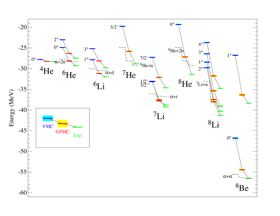
Figure 4: VMC and GFMC energies using AV18/UIX compared to experiment. Black dashed lines show the indicated breakup thresholds for each method. The Monte Carlo statistical errors are shown by the light blue and yellow bands.

Table 4 shows the GFMC energy values for several Hamiltonians. The table and Fig. 4 show that the AV18/UIX Hamiltonian, which gives excellent energies, compared to experiment, for the s-shell nuclei, significantly underbinds the p-shell nuclei. The Li isotopes are stable against breakup into subclusters with AV18/UIX, but progressively more underbound as $A$ increases. There is also an isospin problem, in that the He isotopes are even further off from the experimental values, and in fact do not show stability against breakup into subclusters.

Table 4: GFMC and experimental energies of $A$=3–8 ground states in MeV. Energies of artificially confined 7- and 8-neutron drops are also shown. The experimental values are from Refs. (?, ?, ?).

	AV18	AV18/UIX	AV18/IL2	Expt.
3H($\textstyle{1\over 2}^{+}$)	$-$7.61(1)	$-$8.46(1)	$-$8.43(1)	$-$8.48
4He(0+)	$-$24.07(4)	$-$28.33(2)	$-$28.37(3)	$-$28.30
6He(0+)	$-$23.9(1)	$-$28.1(1)	$-$29.4(1)	$-$29.27
6Li(1+)	$-$26.9(1)	$-$31.1(1)	$-$32.3(1)	$-$31.99
7He($\textstyle{3\over 2}^{-}$)	$-$21.2(2)	$-$25.8(2)	$-$29.2(3)	$-$28.82
7Li($\textstyle{3\over 2}^{-}$)	$-$31.6(1)	$-$37.8(1)	$-$39.6(2)	$-$39.24
8He(0+)	$-$21.6(2)	$-$27.2(2)	$-$31.3(3)	$-$31.41
8Li(2+)	$-$31.8(3)	$-$38.0(2)	$-$42.2(2)	$-$41.28
8Be(0+)	$-$45.6(3)	$-$54.4(2)	$-$56.6(4)	$-$56.50
7n($\textstyle{1\over 2}^{-}$)	$-$33.47(5)	$-$33.2(1)	$-$35.8(2)
8n(0+)	$-$39.21(8)	$-$37.8(1)	$-$41.1(3)

The new Illinois three-nucleon potentials were constructed to solve the p-shell binding problems. Figure 5 and Table 4 compare GFMC calculations for AV18 with no $V_{ijk}$ and AV18/IL2 to the same experimental energies shown in Fig. 4. The AV18/IL2 Hamiltonian does a good job of reproducing these energies; the rms deviation from experiment for these levels is only 360 keV, while it is 2.3 MeV for AV18/UIX. The AV18 values with no $V_{ijk}$ show the large contribution that three-nucleon potentials make to these binding energies; for $A=8$ the IL2 increases the binding energy by more than 10 MeV.

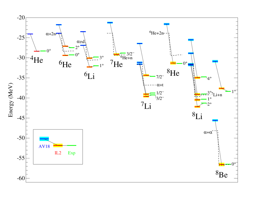
Figure 5: GFMC energies using AV18 and AV18/IL2 compared to experiment.

Table 5 shows some splittings for states that in a simple shell-model picture have the same $L$ and $S$ but different total $J$. In all cases the lowest state for each $J$ is used. Some of the states, particularly the ⁵He states, have large experimental widths; calculations such as those described in Sec. 7 would be more reliable. The splittings are computed for the AV18, AV18/UIX, and AV18/IL2 Hamiltonians and are compared to experimental values. The AV18 with no $V_{ijk}$ significantly underpredicts all the splittings except the $\textstyle{1\over 2}^{-}-\textstyle{3\over 2}^{-}$ doublet in ⁷Li; however in this case the relatively large statistical error for the small splitting makes any conclusion difficult (the computed splittings are the difference of two independent GFMC calculations whose statistical errors must be added in quadrature). The AV18/UIX Hamiltonian substantially improves the ⁵He splitting, and a VMC study showed that an earlier Urbana $V_{ijk}$ significantly increased the computed splitting in ¹⁵N, resulting in much better agreement with experiment (?). However the other splittings in the table are still underpredicted with AV18/UIX. The AV18/IL2 results in good predictions of all the splittings except for the 1${}^{+}-2^{+}$ doublet in ⁸Li which is overpredicted.

Table 5: GFMC and experimental (?, ?) splittings of states with the same $L$ and $S$ but different $J$, in MeV.

		$L$	$S$	AV18	AV18/UIX	AV18/IL2	Expt.
5He	$\textstyle{1\over 2}^{-}-\textstyle{3\over 2}^{-}$	1	$\textstyle{1\over 2}$	0.6(1)	1.1(2)	1.3(2)	1.20
6Li	2${}^{+}-3^{+}$	2	1	0.8(1)	0.9(1)	2.2(2)	2.12
7Li	$\textstyle{1\over 2}^{-}-\textstyle{3\over 2}^{-}$	1	$\textstyle{1\over 2}$	0.5(2)	0.3(2)	0.6(3)	0.47
7Li	$\textstyle{5\over 2}^{-}-\textstyle{7\over 2}^{-}$	3	$\textstyle{1\over 2}$	0.7(2)	0.8(2)	2.2(3)	2.05
8Li	1${}^{+}-2^{+}$	1	1	0.2(4)	0.6(2)	1.7(4)	0.98
7n	$\textstyle{3\over 2}^{-}-\textstyle{1\over 2}^{-}$	1	$\textstyle{1\over 2}$	1.65(7)	1.5(1)	2.8(3)

A detailed breakdown of the GFMC ground-state energies for AV18/IL2 into kinetic, two- and three-nucleon interactions is given in Table 6. Because of the extrapolation of the mixed expectation values, Eq.(48), these components are not as accurate as the total energy, and do not add up to the full amount; indeed the sum of the individual kinetic and potential energies differs from $\langle H\rangle$ by the same amount that the GFMC has improved the $\Psi_{T}$ energy. Nevertheless, they give a good idea about the relative size of the different terms involved. There is a big cancellation between the kinetic and two-body potential terms. Consequently, while $V_{ijk}$ is less than 8% of $v_{ij}$ in magnitude, its expectation value is up to 50% of the net binding (however the net effect of the IL2 $V_{ijk}$, defined as the difference of the binding energies computed without and with $V_{ijk}$, is at most 30%, as can be seen in Table 4). This difference between expectation value and net effect is due to the large change that $V_{ijk}$ induces in $\langle K+v_{ij}\rangle$.

Table 6: Kinetic, $K$, and potential energy contributions in MeV. Shown are the total NN and NNN potential energies, $v_{ij}$ and $V_{ijk}$; the electromagnetic, $v^{\gamma}_{ij}$, and one-pion, $v^{\pi}_{ij}$, parts of $v_{ij}$; and the two- and three-pion parts of $V_{ijk}$.

	$K$	$v_{ij}$	$V_{ijk}$	$v^{\gamma}_{ij}$	$v^{\pi}_{ij}$	$V^{2\pi}_{ijk}$	$V^{3\pi}_{ijk}$
3H	51.	$-$59.	$-$1.5	0.04	$-$45.	$-$3.0	0.18(1)
4He	115.(1)	$-$136.(1)	$-$8.4(1)	0.86	$-$105.	$-$16.3(1)	0.63(1)
6He	147.(2)	$-$171.(2)	$-$11.5(3)	0.87	$-$127.(1)	$-$20.3(4)	$-$0.91(6)
6Li	160.(2)	$-$187.(2)	$-$11.1(3)	1.73	$-$150.(1)	$-$19.8(4)	$-$0.44(5)
7He	175.(3)	$-$199.(3)	$-$16.3(4)	0.89	$-$145.(2)	$-$25.(1)	$-$3.1(1)
7Li	199.(3)	$-$232.(3)	$-$14.5(4)	1.80	$-$178.(2)	$-$25.6(6)	$-$1.1(1)
8He	190.(3)	$-$218.(3)	$-$16.3(5)	0.89	$-$153.(1)	$-$25.6(6)	$-$4.0(1)
8Li	242.(2)	$-$278.(2)	$-$20.6(4)	1.93	$-$211.(1)	$-$34.2(5)	$-$3.8(1)
8Be	256.(4)	$-$303.(3)	$-$21.(1)	3.32	$-$234.(2)	$-$38.5(9)	$-$0.9(2)
7n	105.(1)	$-$59.(1)	$-$3.6(3)	0.07	$-$10.	$-$0.1(1)	$-$5.4(3)
8n	122.(1)	$-$73.(1)	$-$3.0(3)	0.09	$-$12.	0.3(1)	$-$5.9(4)

Among the subcomponents of $v_{ij}$, the one-pion exchange dominates, being 70–80% of the total $v_{ij}$ for $A\geq 3$ nuclei. Similarly, the two-pion exchange is the dominant component of $V_{ijk}$. The three-pion exchange term is small and repulsive in s-shell nuclei, but attractive in the p-shell nuclei, which have $T=\textstyle{3\over 2}$ triples. It is this term which results in the large improvement of the Illinois models over the Urbana models for p-shell nuclei; however its contributions are always less than 15% of the two-pion $V_{ijk}$. Finally, we note that the electromagnetic $v^{\gamma}_{ij}$ is dominated by the Coulomb interaction between protons, but about 17% (8%) of its total contribution comes from the magnetic moment and other terms in He (Li) isotopes.

Table 7: GFMC isovector and isotensor energy coefficients, $a_{n}(A,T)$, [Eq. (52)] computed using AV18/IL2, in keV. The contributions shown are kinetic energy, $K^{CSB}$; Coulomb potential, $v_{C1}(pp)$; other electromagnetic, $v^{\gamma,R}$; and nuclear potential, $v^{CSB}+v^{CD}$. The experimental value for $a_{2}(8,1)$ is extracted using 16.80 MeV as the excitation of the pure $T=1$ isobaric analog state in ⁸Be (?).

$a_{n}(A,T)$	$K^{CSB}$	$v_{C1}(pp)$	$v^{\gamma,R}$	$v^{CSB}+v^{CD}$	Total	Expt.
$a_{1}(3,\textstyle{1\over 2})$	14	649(1)	29	64(0)	757(1)	764
$a_{1}(6,1)$	16	1091(5)	18	47(1)	1172(6)	1173
$a_{2}(6,1)$		166(1)	19	107(13)	293(13)	223
$a_{1}(7,\textstyle{1\over 2})$	22	1447(6)	40	79(2)	1588(7)	1644
$a_{1}(7,\textstyle{3\over 2})$	18	1337(6)	12	52(1)	1420(8)	1373
$a_{2}(7,\textstyle{3\over 2})$		137(1)	7	36(6)	180(7)	175
$a_{1}(8,1)$	23	1686(5)	24	76(1)	1810(6)	1770
$a_{2}(8,1)$		141(1)	4	$-$3(8)	143(8)	128
$a_{1}(8,2)$	18	1528(7)	17	59(1)	1622(8)	1659
$a_{2}(8,2)$		136(1)	6	38(5)	180(5)	153

Energy differences among isobaric analog states are probes of the charge-indepen-dence-breaking parts of the Hamiltonian. The understanding of these “Nolen-Schiffer energies” has been a theoretical problem for 30 years (?). The energies for a given isomultiplet of states can be expanded as

$$E_{A,T}(T_{z})=\sum_{n\leq 2T}a_{n}(A,T)Q_{n}(T,T_{z})\ ,$$ (52)

where $Q_{0}=1$, $Q_{1}=T_{z}$, and $Q_{2}=\textstyle{1\over 2}(3T_{z}^{2}-T^{2})$ are isoscalar, isovector, and isotensor terms (?). The isovector and isotensor coefficients $a_{n}(A,T)$, and various contributions to them, are given in Table 7. These were calculated as expectation values in the $T_{z}=-T$ GFMC wave functions for AV18/IL2. The individual terms are: 1) the effect of the neutron-proton mass difference on the kinetic energy, $K^{CSB}$; 2) the proton-proton Coulomb potential, including the AV18 form factor, $v_{C1}(pp)$; 3) all other electromagnetic terms such as vacuum polarization and magnetic-moment terms, $v^{\gamma,R}$; and 4) the strong-interaction contributions, $v^{CSB}$ which contributes to the isotensor coefficients and $v^{CD}$ which contributes to the isovector coefficients.

The ³H–³He mass difference is 757 keV with the AV18/IL2 Hamiltonian, in excellent agreement with the experimental value of 764 keV. The bulk of the difference is the $pp$ Coulomb energy, but 108 keV comes from the other terms. Because of its very long range, the $v_{C1}(pp)$ dominates the $a_{1}(A,T)$ of heavier nuclei even more and small errors in the rms radius of the nucleus can result in changes in the $v_{C1}(pp)$ contribution that can totally mask the effects of the other, much smaller, terms.

Table 8: VMC isospin-mixing matrix elements for ⁸Be in keV computed using AV18/UIX. Experimental values are from Ref. (?)

$J^{\pi}$	$K^{CSB}$	$v_{C1}(pp)$	$v^{\gamma,R}$	$v^{CSB}$	$E_{01}$	Expt.
2+	2	62	19	26	109(4)	149
1+	1	39	0	15	55(2)	120
3+	1	33	15	13	62(2)	63

Two (2⁺;0+1) states occur very close together in the spectrum of ⁸Be at 16.6 and 16.9 MeV excitation; these isospin-mixed states come from blending the (2⁺;1) isobaric analog of the ⁸Li ground state with the second (2⁺;0) excited state. There are also fairly close (1⁺;0,1) and (3⁺;0,1) pairs at slightly higher energies in the ⁸Be spectrum. The isospin-mixing matrix elements that connect these pairs of states,

$$E_{01}(J)=\langle\Psi(J^{+};0)|H|\Psi(J^{+};1)\rangle\ ,$$ (53)

have been computed using VMC wave functions for the AV18/UIX Hamiltonian. Results for the $E_{01}(J)$ are given in Table 8. The experimental values are determined from the observed decay widths and energies (?). The dominant contribution, from the Coulomb potential, typically accounts for less than half of the matrix element. We see that the remaining part of the electromagnetic interaction and the strong CSB interaction can provide a significant boost, although the experimental mixing is still underpredicted by $\sim$20%. It appears that these mixing elements are a more sensitive test of the small CSB components of the Hamiltonian than are the isobaric analog energy differences.

6 DENSITY AND MOMENTUM DISTRIBUTIONS

The one- and two-nucleon distributions of light $p$-shell nuclei are interesting in a variety of experimental settings. For example, the Borromean ⁶He and ⁸He nuclei are popular candidates for study as ‘halo’ nuclei whose last neutrons are weakly bound. In addition, the polarization densities of ⁶Li and ⁷Li are important because of possible applications in polarized targets.

Table 9: GFMC values for point proton rms radii (in fm) and quadrupole moments (in fm²) in impulse approximation, computed with AV18/IL2. Experimental values are from Refs. (?, ?, ?, ?)

	$\langle r^{2}_{p}\rangle^{1/2}$		$Q$
	GFMC	Expt.	GFMC	Expt.
3H	1.59(0)	1.60
3He	1.76(0)	1.77
4He	1.45(0)	1.47
6He	1.91(1)
6Li	2.39(1)	2.43	–0.32(6)	–0.083
7Li	2.25(1)	2.27	–3.6(1)	–4.06
7Be	2.44(1)		–6.1(1)
8He	1.88(1)
8Li	2.09(1)		3.2(1)	3.11(5)
8B	2.45(1)		6.4(1)	6.8(2)

Point proton rms radii and quadrupole moments are shown in Table 9, as computed by GFMC for the AV18/IL2 model, along with experimental values. The experimental charge radii have been converted to point proton radii by removing the proton and neutron $\langle r^{2}\rangle$ of 0.743 and –0.116 fm², respectively. The radii are in good agreement with experiment, thanks at least in part to the fact that the AV18/IL2 model reproduces the binding energies of these nuclei very well. The quadrupole moments have been calculated in impulse approximation; two-body charge contributions are expected to provide only a few percent correction. The agreement with experiment is again fairly good, with the exception of the ⁶Li quadrupole moment, which involves a delicate cancellation between the contributions from the deuteron quadrupole moment and the D-wave part of the $\alpha$+$d$ relative wave function. In general, quadrupole moments are difficult to calculate accurately with quantum Monte Carlo methods because they are dominated by the long-range parts of the wave functions, which contribute very little to the total energy that VMC and GFMC are both designed to optimize.

Table 10: GFMC values for isoscalar and isovector magnetic moments (in $\mu_{N}$) in impulse approximation using AV18/IL2. Experimental values are from Refs. (?, ?, ?, ?)

	T	Isoscalar		Isovector
		GFMC	Expt.	GFMC	Expt.
3He$-^{3}$H	$\textstyle{1\over 2}$	0.403(0)	0.426	$-$4.330(1)	$-$5.107
6Li	0	0.817(1)	0.822
7Be$-^{7}$Li	$\textstyle{1\over 2}$	0.894(1)	0.929	$-$3.93(1)	$-$4.654
8B$-^{8}$Li	1	1.276(1)	1.345	0.369(9)	$-$0.309

Calculated and experimental isoscalar and isovector magnetic moments are shown in Table 10, as defined with the convention used in Eq.(52); thus the isovector values for the $T=\textstyle{1\over 2}$ cases are $-$2 times those often quoted in the literature. (For the $A=8$, $T=1$ nuclei the experimental isoscalar and isovector moments are obtained from the sum and difference of the values for B and Li, since the magnetic moment of the $T=1$ $J^{\pi}=2^{+}$ state in Be is not measured.) The moments were calculated as expectation values in the GFMC wave functions with $T_{z}=-T$ in impulse approximation. These impulse isoscalar moments are quite close to experiment and it is expected that two-body current contributions are small (?). For isovector moments, however, there can be significant corrections from meson-exchange contributions. We note that the corrections needed for the $A$=7,8 isovector moments are the same sign and magnitude as for $A$=3, so an exchange-current model that fixes the s-shell (?) is likely to work for the light p-shell nuclei also.

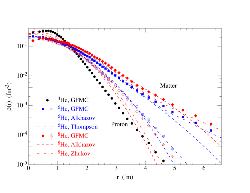
Figure 6: Proton and matter densities in ⁴He, ⁶He, and ⁸He. Analyses of ^6,8He-proton scattering are shown by the dashed (Ref. (?)) and dot-dashed (Ref. (?)) curves.

In Fig. 6, we present proton and matter (proton$+$neutron) densities for the stable helium isotopes, as calculated with GFMC for AV18/IL2. Nucleon densities are calculated as simple $\delta$-function expectation values, with possible spin and/or isospin projectors: for example, the proton density is given by

$$\rho_{p}(r)\ =\ \frac{1}{4\pi r^{2}}\langle\Psi|\sum_{i}\ \ \frac{1+\tau_{zi}}{2}\ \delta(r-|{\bf r}_{i}-{\bf R}_{cm}|)\ |\Psi\rangle\ .$$ (54)

The blue symbols and curves show results for ⁶He, red ones for ⁸He; open symbols give the proton distributions which are also interpreted as the alpha “core” density, full symbols are the total matter densities. It can be seen that, as more neutrons are added, the tails of the matter distributions broaden considerably because of the relatively weak binding of the p-shell neutrons. In addition, the central neutron and proton densities decrease rather dramatically. This effect does not necessarily require any changes to the $\alpha$ core, but can be understood at least partially from the fact that the $\alpha$ no longer sits at the center of mass of the entire system. The motion relative to the center of mass spreads out the mass distribution relative to that of ⁴He.

The figure also shows two attempts to extract the densities of ^6,8He from scattering of beams of these short-lived nuclei from proton targets (?). The analysis of Alkhazov, et al. (dashed curves) used Glauber theory and assumed proton (core) and matter density distributions which were varied to fit the measured cross sections. The later work of Al-Khalili and Tostevin (?) (dot-dashed curves) improved on this by doing the Glauber theory using model wave functions which contained correlations between the valence neutrons. The GFMC calculations definitely prefer the latter analysis.

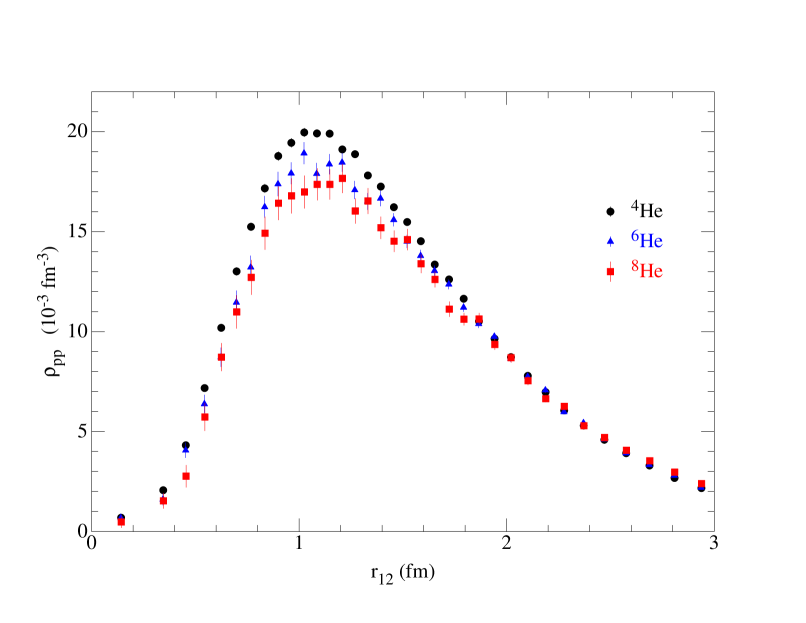
Figure 7: Proton-proton distribution functions in helium isotopes

The proton-proton distribution function is defined by

$$\rho_{pp}(r)=\frac{1}{4\pi r^{2}}\langle\Psi|\sum_{i<j}\ \frac{1+\tau_{zi}}{2}\ \frac{1+\tau_{zj}}{2}\ \delta(r-|{\bf r}_{i}-{\bf r}_{j}|)|\Psi\rangle\ .$$ (55)

These distributions are directly related to the Coulomb sum measured in inclusive longitudinal electron scattering; such measurements in ³He have been used to put constraints on the $\rho_{pp}(r_{ij})$, and realistic calculations agree with the experimental results(?). The behavior of $\rho_{pp}(r)$ at short distances is largely determined by the repulsive core of the $N\!N$ potential and is nearly independent of the nucleus, but at larger distances it is determined by the size of the nucleus.

It is interesting to compare $\rho_{pp}$ for ⁴He to that of ⁶He and ⁸He. These distribution functions are shown in Fig. 7, again calculated with GFMC for the AV18/IL2 model. These nuclei each have just one $pp$ pair which presumably is in the “alpha core” of ^6,8He. Unlike the one-body densities, these distributions are not sensitive to center of mass effects, and thus if the alpha core of ^6,8He is not distorted by the surrounding neutrons, all three $\rho_{pp}$ distributions in the figure should be the same. We see that the $pp$ distribution spreads out slightly with neutron number in the helium isotopes, with an increase of the pair rms radius of approximately 4% in going from ⁴He to ⁶He, and 8% to ⁸He. While this could be interpreted as a swelling of the alpha core, it might also be due to the charge-exchange ($\tau_{i}\cdot\tau_{j}$) correlations which can transfer charge from the core to the valence nucleons. Since these correlations are rather long-ranged, they can have a significant effect on the $pp$ distribution. VMC calculations of ⁴He with wave functions modified to give $\rho_{pp}$ distributions close to those of ^6,8He suggest that the alpha cores of ^6,8He are excited by $\sim 80$ and $\sim 350$ keV, respectively.

In general, VMC calculations give one-body densities very similar to the GFMC results, although the two-body densities may differ by up to 10% in the peak, with the GFMC having a somewhat sharper structure. Because the VMC wave functions are simpler and less expensive to construct they have been used in a number of applications where the single-particle structure is dominant. All these calculations were carried out with wave functions for the AV18/UIX Hamiltonian, but we expect that GFMC calculations with the improved AV18/IL2 model will not qualitatively alter the results. (Remember that the VMC wave functions are constrained to reproduce available experimental rms radii.)

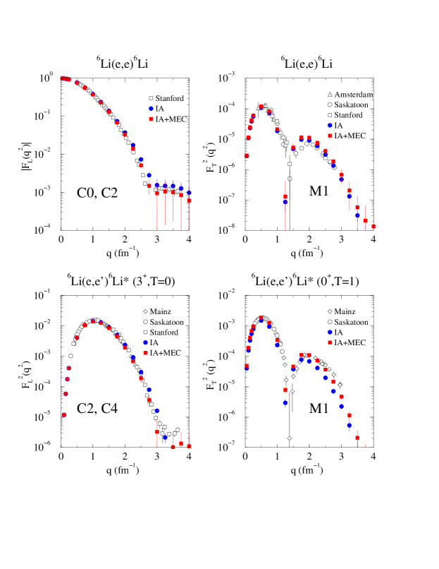
Figure 8: Calculated and experimental elastic and transition form factors in ⁶Li. Experimental data are from Refs. (?, ?, ?, ?, ?, ?, ?).

VMC calculations of elastic and inelastic electromagnetic form factors for ⁶Li are shown in Fig. 8. These have been made in impulse approximation (IA) and with meson-exchange contributions (MEC) to the charge and density operators (?). The comparison with data for the elastic longitudinal form factor, $F_{L}(q^{2})$, is excellent, as is the E2 transition to the 3⁺ first excited state. The MEC corrections are small, but stand out noticeably in the first minimum where they significantly improve the fit to data. The elastic transverse form factor, $F_{T}(q^{2})$, is good up to the first zero, but is a little too large in the region of the second maximum. The M1 transition to the 0⁺ isobaric analog state is also reproduced reasonably well. This kind of quantitative agreement with data has not been achieved in the past with either shell model or $\alpha$+$d$ cluster wave functions. In fact, shell model calculations normally require the introduction of effective charges, typically adding a charge of $\sim 0.5e$ to both the proton and neutron, to obtain reasonable transition rates (?). No effective charges are used in the VMC calculations.

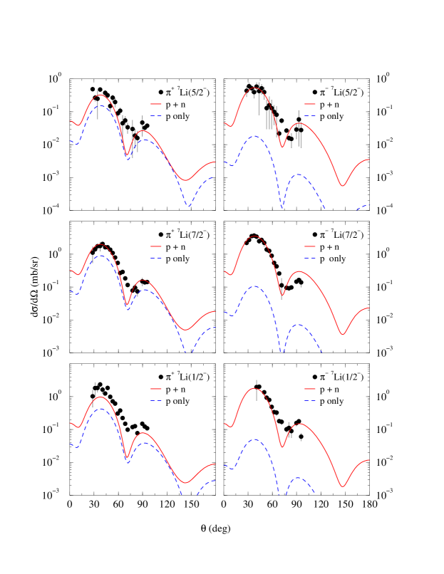
Figure 9: Differential cross sections for ⁷Li$(\pi,\pi^{\prime})$ scattering at $E_{\pi}=164$ MeV. Data are from Ref. (?).

While electron scattering from nuclei is primarily sensitive to the proton distributions in nuclei, $\pi^{-}$ scattering is most sensitive to the neutron distributions. Pion inelastic scattering at medium energy ($80\leq E_{lab}\leq 300$ MeV) is dominated by strong absorption due to excitation of the $\Delta$ resonance, and is well described in distorted-wave impulse approximation (DWIA). An analysis of meson factory data for p-shell nuclei based on the Cohen-Kurath shell model (?) showed that reasonable agreement with data could be achieved if the quadrupole excitation operator was enhanced by a factor $\sim$ 1.75–2.5 (?). Figure 9 shows a calculation of the differential cross sections for ⁷Li($\pi,\pi^{\prime}$) scattering to the first three excited states using VMC transition densities as input, with no enhancement factors (?). Solid red lines show the full results, which are in good agreement with the data, while the dashed blue lines give the contribution coming from protons only. Because of the strong isospin dependence of the $\pi N$ scattering $t$-matrix, this reaction can be a stringent test of the neutron densities predicted by the quantum Monte Carlo calculations.

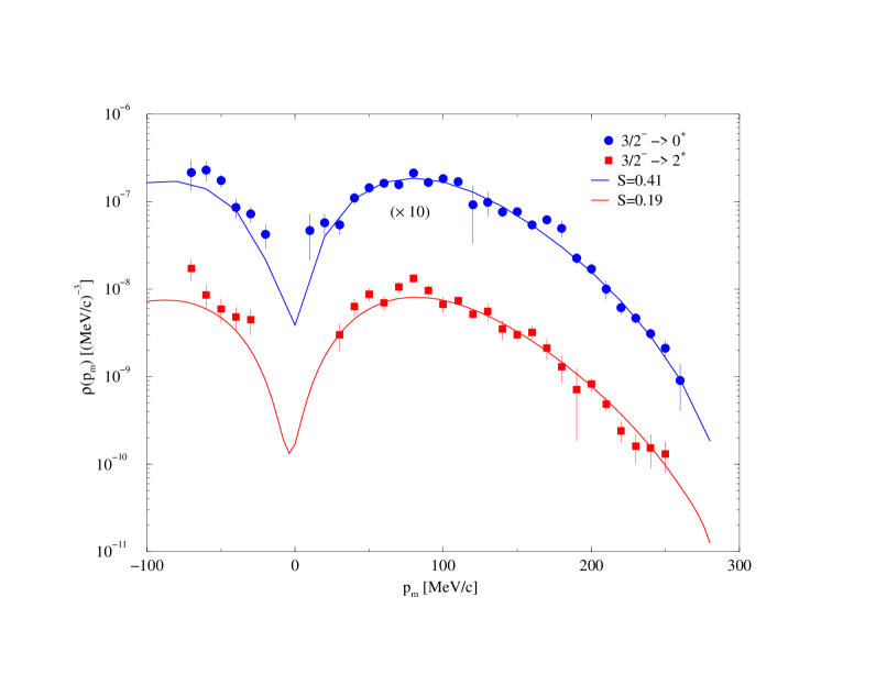
Figure 10: Experimental (?) momentum distributions for the transitions to the ground state (circles) and first excited state (squares) in the reaction ⁷Li$(e,e^{\prime}p)^{6}$He, compared to CDWIA calculations with the VMC wave functions (solid lines) for AV18/UIX.

The VMC wave functions for the AV18/UIX model have also been used to calculate single-nucleon momentum distributions in many nuclei, and a variety of cluster-cluster overlap wave functions, such as $\langle dp|t\rangle$, $\langle dd|\alpha\rangle$, and $\langle\alpha d|^{6}{\rm Li}\rangle$ (?, ?). Recently the overlaps $\langle^{6}{\rm He}(J^{\pi})+p(\ell_{j})|^{7}{\rm Li}\rangle$ for all possible p-shell states in ⁶He were studied (?). The spectroscopic factors obtained from these overlaps are 0.41 to the ground state of ⁶He and 0.19 to the 2⁺ first excited state. These factors are significantly smaller than the predictions of the Cohen-Kurath shell model (?), which gives values of 0.59 and 0.40, respectively. The CK shell model requires that the possible ⁶He$+p$ states sum to unity within the p-shell, whereas in the VMC calculation, the correlations in the wave function push significant strength to higher momenta that cannot be represented as a ⁶He state plus p-wave proton. The VMC overlaps were used as input to a Coulomb DWIA analysis of recent ⁷Li$(e,e^{\prime}p)^{6}$He data taken at NIKHEF (?) and found to give an excellent fit to the data, as shown in Fig. 10.

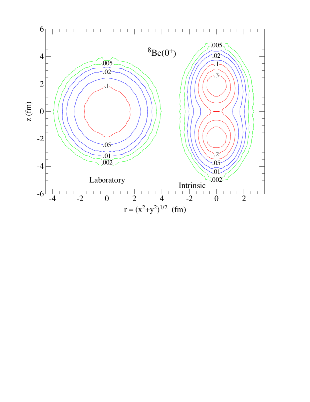
Figure 11: Calculated density contours of ⁸Be in the lab frame (left) and the intrinsic frame (right), labeled with densities in fm^-3

The VMC wave functions are based on one-body parts that have a shell-model structure, namely four nucleons in an $\alpha$ core coupled to $(A-4)$ one-body $\ell=1$ wave functions. However the low-lying states of ⁸Be exhibit a rotational spectrum and are believed to be well approximated as two $\alpha$’s rotating around their common center of mass. It is possible to recover this picture from the VMC wave functions by a modified Monte Carlo density calculation (?).

The standard Monte Carlo method for computing one-body densities, $\rho({\bf r})$, is to make a random walk that samples $|\Psi({\bf r}_{1},{\bf r}_{2},\cdots,{\bf r}_{A})|^{2}$ and to bin ${\bf r}_{1},{\bf r}_{2},\cdots,{\bf r}_{A}$ for each configuration in the walk. The density is then proportional to the number of samples in each bin. In the case of a $J$ = 0 nucleus, this “laboratory” density will necessarily be spherically symmetric.

The intrinsic density in body-fixed coordinates can be approximated by computing the moment of inertia matrix, ${\cal M}$, of the $A$ positions for each configuration. The eigenvalues and eigenvectors of ${\cal M}$, are found and a rotation to those principal axes is made. The resulting ${\bf r}_{1}^{\prime},{\bf r}_{2}^{\prime},\cdots,{\bf r}_{A}^{\prime}$ is then binned. The eigenvector with the largest eigenvalue is chosen as the ${\bf z}^{\prime}$ axis. This procedure will not produce a spherically symmetric distribution, even if there is no underlying deformed structure, because almost every random configuration will have principal axes of different lengths and the rotation will always orient the longest principal axis in the ${\bf z}^{\prime}$ direction. However no artificial structure is introduced (?).

When the above procedure is applied to the three lowest ⁸Be states, a dramatic intrinsic structure is revealed, as shown in Fig. 11 for the ground state. The figure shows contours of constant density plotted in cylindrical coordinates. The left side of the figure shows the standard, lab frame, density calculation. For the $J$ = 0 ground state, this is spherically symmetric as shown. The right side of the figure shows the intrinsic density. It is clear that the intrinsic density has two peaks, with the neck between them having only one-third the peak density; we regard these as two $\alpha$’s. This assignment is strengthened by making the same construction for the $J=2^{+}$ and $4^{+}$ states; although the laboratory densities for these states (in $M=J$ states) are quite different, the intrinsic densities are, within statistical errors, the same as the $J=0$ intrinsic density (?).

If the $0^{+}$, $2^{+}$, and $4^{+}$ states are generated by rotations of a common deformed structure, then their electromagnetic moments and transition strengths should all be related to the intrinsic moments which can be computed by integrating over the projected body-fixed densities. This is explored in Ref. (?) and a generally consistent picture is shown.

7 LOW-ENERGY NUCLEON-NUCLEUS SCATTERING

The calculations presented so far have treated resonant nuclear states as if they were particle stable; that is the VMC trial wave functions decay exponentially at large distances and the GFMC propagation does not impose a scattering-state boundary condition. As was shown in Fig. 3, this GFMC propagation converges for unstable states that are narrow, but for wide states, such as ⁸Be(4⁺), the $E(\tau)$ keeps decreasing for increasing $\tau$. Such states should be computed using scattering-wave boundary conditions.

The ⁵He($\textstyle{1\over 2}^{-}$, $\textstyle{3\over 2}^{-}$) states have been studied in VMC (?) and GFMC (?) using scattering-wave boundary conditions. The VMC calculations use a trial function that is a straight-forward generalization of the $\Psi_{V}$ given in Sec. 3. In it the $\Psi_{J}$ contains one p-wave single-particle function that goes to zero at a specified (large) radius, $R_{n}$. The variational energy is minimized subject to this boundary condition. The phase shift at the resulting scattering energy, $E_{s}=E(^{5}\mbox{He}(R_{n}))-E(^{4}\mbox{He})$ is then obtained from

$$\tan(\delta_{l})=\frac{j_{l}(kR_{n})}{n_{l}(kR_{n})},$$ (56)

where $k=(2\mu E_{s})^{1/2}/\hbar$, $\mu$ is the $\alpha$+$n$ reduced mass, and $j_{l}$ and $n_{l}$ are the spherical Bessel functions (in this case $l=1$). It is possible to generalize this formulation by specifying a logarithmic-derivative at $R_{n}$, rather than having the wave function go to zero there. This method requires the computation of the energy difference, $E_{s}$. If this is done with two different VMC calculations, one for ⁵He with the specified boundary condition, and one for ⁴He, then the statistical errors of these two calculations must be added in quadrature. Instead one can directly evaluate the energy difference in a VMC random walk that is controlled by the ⁵He wave function. In practice this gives $E_{s}$ with a smaller statistical error than either of the separate statistical errors (?). The GFMC calculations start with the scattering-state trial function and use a modified propagator that preserves the boundary condition (?). Both methods result in a phase shift and energy corresponding to a given boundary condition. By repeating the calculations for different boundary conditions, the phase shift as a function of energy can be mapped out.

The VMC calculations of Ref. (?) used older two- and three-nucleon potentials than have been used for the other calculations reported in this review. They reproduced the qualitative features of the experimental $\alpha$+$n$ $\textstyle{1\over 2}^{-}$ and $\textstyle{3\over 2}^{-}$ phase shifts, but, in particular, gave a spin-orbit splitting about 1 MeV too small. The GFMC calculations (?) used a different, but still somewhat old Hamiltonian and obtained values that are closer to experiment. These calculations need to be repeated with the modern Hamiltonians described in this review, and for other systems such as $\alpha$+$d$, ⁶He+$n$, and $\alpha$+$\alpha$.

8 ASTROPHYSICAL ELECTROWEAK REACTIONS

Most of the key nuclear reactions in primordial nucleosynthesis (?) and solar neutrino production (?) involve only the $A\leq 8$ nuclei. Many of these are electroweak capture reactions that are difficult or impossible to measure in the laboratory. With the high-precision few-body methods, such as PHH and Faddeev, or new effective field theory treatments, the reactions to s-shell final states have been calculated with unprecedented accuracy in the last few years. These include the ¹H$(p,e^{+}\nu_{e})^{2}$H (?) and ³He$(p,e^{+}\nu_{e})^{4}$He (?) weak capture reactions, and the ¹H$(n,\gamma)^{2}$H (?), ²H$(n,\gamma)^{3}$H and ²H$(p,\gamma)^{3}$He (?) radiative capture reactions.

Recently, the VMC method has been applied to some of the radiative captures to p-shell final states, including ²H($\alpha,\gamma)^{6}$Li, ³H($\alpha,\gamma)^{7}$Li, and ³He($\alpha,\gamma)^{7}$Be (?, ?). As discussed in the previous section, many-nucleon scattering states can be constructed within the quantum Monte Carlo framework, but it has not yet been done for $A\geq 6$ nuclei. Thus for these first studies, the appropriate electromagnetic matrix elements (primarily E1 and E2) are evaluated between a VMC six- or seven-nucleon final state, and a correlated cluster-cluster scattering state which is not variationally improved.

Since much of the capture takes place at long range, an important ingredient in these calculations is an asymptotically-correct description of the six- or seven-body final state. This feature has to be implemented in the initial variational wave function because, as remarked before, the VMC and GFMC methods find their best wave functions by optimizing the energy, which is not sensitive to the long-range behavior. The asymptotic behavior can be imposed by requiring the one-body wave function in Eq.(3) to satisfy the condition:

$$[\phi^{LS[n]}_{p}(r\rightarrow\infty)]^{n}\propto W_{km}(2\gamma r)/r\ ,$$ (57)

where $W_{km}(2\gamma r)$ is the Whittaker function for bound-state wave functions in a Coulomb potential and $n$ is the number of p-shell nucleons. Here $\gamma^{2}=2\mu_{4n}B_{4n}/\hbar^{2}$, with $\mu_{4n}$ and $B_{4n}$ the appropriate two-cluster effective mass and binding energy. For ⁶Li, $B_{42}=1.47$ MeV; for ⁷Li or ⁷Be, capture can be to the $\textstyle{3\over 2}^{-}$ ground or $\textstyle{1\over 2}^{-}$ excited state with corresponding values for $B_{43}$.

The initial-state wave functions are taken as elastic-scattering states of the form

$$|\psi_{\alpha\tau};LSJM\rangle={\cal A}\left\{\phi_{\alpha\tau}^{JL}(r_{\alpha\tau})Y_{LM_{L}}({\bf\hat{r}}_{\alpha\tau})\prod_{ij}G_{ij}|\psi_{\alpha}\psi_{\tau}^{m_{S}}\rangle\right\}_{LSJM},$$ (58)

where curly braces indicate angular momentum coupling, $\cal{A}$ antisymmetrizes between clusters, $\psi_{\alpha}$ is the ⁴He ground state, and $\psi_{\tau}^{m_{S}}$ is the deuteron or trinucleon ground state in spin orientation $m_{S}$. The $G_{ij}$ are identity operators if the nucleons $i$ and $j$ are in the same cluster, else, they are a set of pair correlation operators, including both central and spin-isospin dependent terms, which introduce distortions in each cluster, under the influence of individual nucleons from the other cluster. They are similar to the correlations discussed in Sec. 3, except that they revert to the identity operator at pair separations beyond about 2 fm. The correlations $\phi_{\alpha\tau}^{JL}$ are generated from optical potentials that describe the experimental phase shifts in cluster-cluster scattering; see Refs. (?, ?) for details. Because the $G_{ij}$ go to unity, the $\psi_{\alpha\tau}$ has the same phase shifts as those generated by the optical potential.

Evaluation of electromagnetic matrix elements between the initial scattering and final bound states can be split into two parts by noting that all of the energy dependence is contained in the relative wave function $\phi_{\alpha\tau}^{JL}$ and the transition operators. Thus, using a technique first applied in a VMC calculation of $d$+$d$ radiative capture (?), the matrix element for a given scattering partial wave can be written as

$$T^{LSJ_{i}J_{f}}_{\ell}(q) = \int_{0}^{\infty}dx\,x^{2}\,\phi_{\alpha\tau}^{J_{i}L}(x)$$

$$\times \langle\psi_{A}^{J_{f}m_{f}}|T_{\ell\lambda}(q){\cal A}\left\{\delta(x-r_{\alpha\tau})Y_{L}^{M_{L}}({\bf\hat{r}}_{\alpha\tau}))\prod_{ij}G_{ij}|\psi_{\alpha}\psi_{\tau}^{m_{S}}\rangle\right\}_{LSJ_{i}M_{i}}\ ,$$

where $T_{\ell\lambda}$ denotes any of the standard $E_{\ell}$ or $M_{\ell}$ operators. The integration over all coordinates except $x$ can be calculated just once for each partial wave by Monte Carlo sampling, and the result can then be used to compute the full integral for as many energies as desired by recomputing $\phi_{\alpha\tau}^{J_{i}L}(x)$ only.

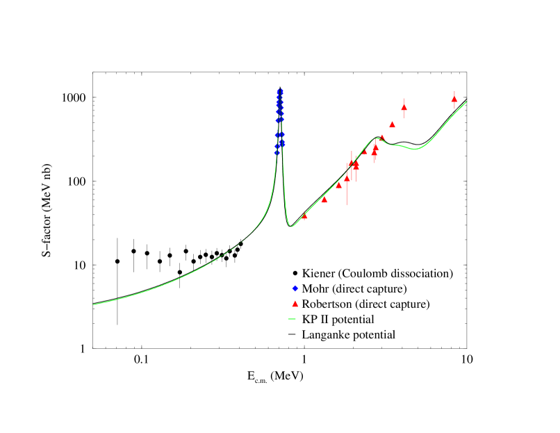
Figure 12: The total $S$-factor for $\alpha$+$d$ radiative capture calculated for two different optical potentials with the AV18/UIX nuclear wave functions, compared to experimental data (?, ?, ?).

The result for the ²H($\alpha,\gamma)^{6}$Li capture $S$-factor is shown in Fig. 12, where it is compared to a collection of direct and indirect data. The $S$-factor falls rapidly at low-energy because a pseudo-orthogonality between the initial and final states suppresses normal S-wave capture. Whenever there is such a suppression, it is important to consider higher-order terms that might contribute, including relativistic corrections and two-body charge and current operators (?). This is possible with the VMC calculation because of the fully correlated $A$-body wave functions that are used. In this case, a relativistic center-of-energy correction leads to an E1 contribution that dominates at low energy, while the resonance region and above is primarily E2. Results for ³H($\alpha,\gamma)^{7}$Li, and ³He($\alpha,\gamma)^{7}$Be can be found in Ref. (?)

This kind of VMC calculation is only a first investigation into the p-shell astrophysical reactions, and should be improved in the future by using the more exact GFMC wave functions for both bound and scattering states, and the Hamiltonians with improved $N\!N\!N$ potentials.

9 NEUTRON DROPS

Neutron-rich nuclei are interesting both because of their importance in various astrophysical contexts, such as the r-process or neutron-star crusts, and the current interest in experiments with radioactive beams. These nuclei are often studied within the framework of mean-field models using Skyrme or other potential models. The parameters of these models are fit to experimentally known binding energies, that is for situations with $N{\sim}Z$. In particular the isospin dependence of the spin-orbit component of such potentials is considered to be not strongly constrained. Neutron drops offer the possibility of theoretical guidance for the isotopic dependence of such parameters.

Neutron drops are systems of interacting neutrons confined in an artificial external well. Eight neutrons form a closed shell and single-particle spin-orbit splittings can be studied in drops of seven or nine neutrons. Pairing energies can be studied if six-neutron drops are also computed. Calculations of systems of seven and eight neutrons interacting with AV18/UIX were used as a basis for comparing Skyrme models of neutron-rich systems with microscopic calculations based on realistic interactions (?). The external one-body well used is a Woods-Saxon:

$$V_{1}(r)=\sum_{i}\frac{V_{0}}{1+\exp[-(r_{i}-r_{0})/a_{0}]}\ ;$$ (60)

the parameters are $V_{0}=-20$ MeV, $r_{0}=3.0$ fm, and $a_{0}=0.65$ fm. Neither the external well nor the total internal potential ($v_{ij}+V_{ijk}$) are individually attractive enough to produce bound states of seven or eight neutrons; however the combination does produce binding.

Tables 4-6 show results for the neutron drops with this external well. The $T=\textstyle{3\over 2}$ nature of the $S^{I}_{\tau}S^{I}_{\sigma}$ term of $V^{3\pi}$ results in large contributions in the neutron drops. As a result the seven-neutron drops computed with AV18/IL2 have double the spin-orbit splitting predicted by AV18/UIX. Thus the spin-orbit splitting in neutron-rich systems depends strongly on the Hamiltonian used.

10 CONCLUSIONS AND OUTLOOK

Quantum Monte Carlo methods can now be used to obtain accurate (within 2%) energies for light p-shell nuclei up to $A$ = 8. Initial calculations of $A$=9,10 nuclei have been made by the authors, and studies of $A$=11,12 nuclei should be feasible in the next few years by variational and Green’s function Monte Carlo methods. This progress in the nuclear many-body problem is due both to the rapid growth of computational power and the continuing evolution of algorithms. The new auxiliary-field diffusion Monte Carlo method, which samples spins and isospins by auxiliary fields, and space by standard diffusion Monte Carlo, may be the key to doing even larger nuclear systems (?).

Studies of the p-shell nuclei allow us to test nuclear forces in new ways not accessible in s-shell nuclei, particularly the odd partial waves of $N\!N$ scattering and the $T=\textstyle{3\over 2}$ triples for $N\!N\!N$ forces. They also give us many more cases in which to examine charge-dependent and charge-symmetry-breaking interactions. With these calculations of nuclear spectra, we see for the first time that nuclear structure, including both single-particle and clustering aspects, really can be explained directly in terms of bare nuclear forces that fit $N\!N$ data. A crucial ingredient for quantitative agreement is the addition of realistic $N\!N\!N$ forces, including at least two terms beyond the standard long-range two-pion-exchange potential (?).

Many aspects of nuclear structure and reactions are described quantitatively in these studies. The energy differences between isobaric analog states are explained well once the complete electromagnetic and strong charge-independence-breaking forces deduced from $N\!N$ scattering are included. Charge radii and quadrupole moments agree with experiment, and we expect magnetic moments will also once the important two-body exchange currents are included, as they have been in s-shell nuclei (?). Elastic and transition form factors measured in electron scattering, and transition densities that are tested in pion scattering, are accurately predicted without the introduction of effective charges. Spectroscopic factors are naturally quenched by the correlations in $A$-body wave functions and we see that those correlations build up intrinsic cluster structure, as in the case of ⁸Be.

Initial calculations of nucleon-nucleus scattering states and electroweak capture reactions are encouraging. These two related problems will be a major activity for the quantum Monte Carlo studies over the next several years, with studies of scattering states in nuclei like ⁷He and ⁹He, and of the cluster-cluster scattering states that enter into the astrophysical capture reactions. Additional reactions like ⁷Be$(p,\gamma)^{8}$B and even ⁸Be$(\alpha,\gamma)^{12}$C should become feasible. Still other projects will include the study of weak decays and, going beyond the p-shell, looking at the unnatural-parity intruder states which start to dip into the low-energy spectrum with the $A=9$ nuclei, and can be particle stable by $A=10$.

Refining the nuclear Hamiltonian will remain a major aspect of future work. Extensive new $N\!N$ scattering data taken since the Nijmegen partial-wave analysis has increased the database to more than 6000 points, and a new CD-Bonn 2000 potential has been constructed that again achieves a $\chi^{2}/$datum $\approx 1$ (?). Also, intensive searches are being made to look for $N\!N\!N$ force signatures in $N+d$ scattering experiments (?, ?), which may well indicate a need for additional terms beyond those contained in the Illinois models. Our ability to test new force models, as they become available, in light nuclei by accurate quantum Monte Carlo methods will continue to be an important tool for nuclear physics.

References

- 1. Stoks VGJ, Klomp RAM, Rentmeester MCM, de Swart JJ. Phys. Rev. C 48:792 (1993)
- 2. Chen CR, Payne GL, Friar JL, Gibson BF. Phys. Rev. C 31:2266 (1985)
- 3. Carlson J. Phys. Rev. C 36:2026 (1987)
- 4. Carlson J, Schiavilla R. Rev. Mod. Phys. 70:743 (1998)
- 5. Cohen S, Kurath D. Nucl. Phys. 73:1 (1965)
- 6. Kuo TTS, Brown GE. Nucl. Phys. 85:40 (1966)
- 7. Navratil P, Vary JP, Barrett BR. Phys. Rev. Lett. 84:5728 (2000)
- 8. Lomnitz-Adler J, Pandharipande VR, Smith RA. Nucl. Phys. A361:399 (1981)
- 9. Carlson J, Pandharipande VR, Wiringa RB. Nucl. Phys. A401:86 (1983)
- 10. Wiringa RB. Phys. Rev. C 43:1585 (1991)
- 11. Arriaga A, Pandharipande VR, Wiringa RB. Phys. Rev. C 52:2362 (1995)
- 12. Wiringa RB, Schiavilla R. Phys. Rev. Lett. 81:4317 (1998)
- 13. Lapikás L, Wesseling J, Wiringa RB. Phys. Rev. Lett. 82:4404 (1999)
- 14. Lee T-SH, Wiringa RB. Phys. Rev. C 63:014006 (2001)
- 15. Nollett KM, Wiringa RB, Schiavilla R. Phys. Rev. C 63:024003 (2001)
- 16. Nollett KM. nucl-th/0102022, submitted to Phys. Rev. C
- 17. Pudliner BS, Pandharipande VR, Carlson J, Wiringa RB. Phys. Rev. Lett. 74:4396 (1995)
- 18. Pudliner BS, et al. Phys. Rev. C 56:1720 (1997)
- 19. Wiringa RB, Pieper SC, Carlson J, Pandharipande VR. Phys. Rev. C 62:014001 (2000)
- 20. Schmidt KE, Fantoni S. Phys. Lett. B 446:99 (1999)
- 21. Wiringa RB, Stoks VGJ, Schiavilla R. Phys. Rev. C 51:38 (1995)
- 22. Pieper SC, Pandharipande VR, Wiringa RB, Carlson J, nucl-th/0102004, submitted to Phys. Rev. C
- 23. Metropolis N, et al. J. Chem. Phys. 21:1087 (1953)
- 24. Stoks VGJ, de Swart JJ. Phys. Rev. C 47:761 (1993); Phys. Rev. C 52:1698 (1995)
- 25. Stoks VGJ, Klomp RAM, Terheggen CPF, de Swart JJ. Phys. Rev. C 49:2950 (1994)
- 26. Machleidt R, Sammarruca F, Song Y. Phys. Rev. C 53:R1483 (1996)
- 27. Fujita J, Miyazawa H. Prog. Theor. Phys. 17:360 (1957)
- 28. Coon SA, et al. Nucl. Phys. A317:242 (1979)
- 29. Coelho HT, Das TK, Robilotta MR. Phys. Rev. C 28:1812 (1983)
- 30. Friar JL, Hüber D, van Kolck U. Phys. Rev. C 59:53 (1999)
- 31. Carlson J, Pandharipande VR, Schiavilla R. Phys. Rev. C 47:484 (1993)
- 32. Forest JL, Pandharipande VR, Carlson J, Schiavilla R. Phys. Rev. C 52:576 (1995)
- 33. Forest JL, Pandharipande VR, Arriaga A. Phys. Rev. C 60:014002 (1999)
- 34. Forest JL, Pandharipande VR, Friar JL. Phys. Rev. C 52:568 (1995)
- 35. Friar JL. Phys. Rev. C 12:695 (1975)
- 36. Wiringa RB. Rev. Mod. Phys. 65:231 (1993)
- 37. Bohr A, Mottelson BR. Nuclear Structure Volume I. New York: W. A. Benjamin (1969)
- 38. Carlson JA, Wiringa RB. Computational Nuclear Physics 1, ed. K Langanke, JA Maruhn, SE Koonin. Berlin: Springer (1991)
- 39. Pudliner BS, et al. Phys. Rev. Lett. 76:2416 (1996)
- 40. Smerzi A, Ravenhall DG, Pandharipande VR. Phys. Rev. C 56:2549 (1997)
- 41. Carlson J. private communication
- 42. Carlson J. Phys. Rev. C 38:1879 (1988)
- 43. Ceperley DM. Rev. Mod. Phys. 67:279 (1995)
- 44. Kalos MH. J. Comp. Phys. 2:257 (1967)
- 45. Ceperley DM, Kalos MH. Monte Carlo Methods in Statistical Physics, ed. K. Binder. Heidelberg: Springer (1979)
- 46. Zhang S, Carlson J, Gubernatis JE. Phys. Rev. Lett. 74:3652 (1995)
- 47. Friar JL, Payne GL, Stoks VGJ, de Swart JJ. Phys. Lett. B 311:4 (1993)
- 48. Nogga A, Kamada H, Glöckle W. Phys. Rev. Lett. 85:944 (2000)
- 49. Kievsky A, Marcucci LE, Rosati S, Viviani M. Few-Body Syst. 22:1 (1997)
- 50. Viviani M, Kievsky A, Rosati S. Few-Body Syst. 18:25 (1995)
- 51. Kievsky A, Viviani M, Rosati S. Nucl. Phys. A551:241 (1993)
- 52. Kievsky A. private communication
- 53. Tilley DR, Weller HR, Hasan HH. Nucl. Phys. A474:1 (1987)
- 54. Tilley DR, Weller HR, Hale GM. Nucl. Phys. A541:1 (1992)
- 55. Ajzenberg-Selove F. Nucl. Phys. A490:1 (1988)
- 56. Pieper SC, Pandharipande VR. Phys. Rev. Lett. 70:2541 (1993)
- 57. Tilley DR, et al. TUNL preprint “Energy Levels of Light Nuclei A = 5,6,7” (2001)
- 58. Nolen JA, Schiffer, JP. Ann. Rev. Nucl. Sci. 19:471 (1969)
- 59. Peshkin M. Phys. Rev. 121:636 (1960)
- 60. Barker FC. Nucl. Phys. 83:418 (1966)
- 61. De Vries H, De Jager CW, De Vries C. At. Data Nucl. Data Tables 36:495 (1987)
- 62. Shiner D, Dixson R, Vedantham V. Phys. Rev. Lett. 74:3553 (1995)
-
63.
Raghavan P.
At. Data Nucl. Data Tables 42:189 (1989);
Stone N. www.nndc.bnl.gov/nndc/stone_moments/moments.html (1997) - 64. Schiavilla R, Pandharipande VR, Riska DO. Phys. Rev. C 40:2294 (1989)
- 65. Marcucci LE, Riska DO, Schiavilla R. Phys. Rev. C 58:3069 (1998)
- 66. Alkhazov GD, et al.. Phys. Rev. Lett. 78:2313 (1997)
- 67. Al-Khalili JS, Tostevin JA. Phys. Rev. C 57:1846 (1998)
- 68. Schiavilla R, Wiringa RB, Carlson J. Phys. Rev. Lett. 70:3856 (1993)
- 69. Li GC, Sick I, Whitney RR, Yearian MR. Nucl. Phys. A162:583 (1971)
- 70. Lapikás L. Proceedings of the Conference on Modern Trends in Elastic Electron Scattering, ed. C De Vries. Amsterdam:NIKHEF-K (1978)
- 71. Bergstrom JC, Kowalski SB, Neuhausen R. Phys. Rev. C 25:1156 (1982)
- 72. Rand RE, Frosch R, Yearian MR. Phys. Rev. 144:859 (1966)
- 73. Bergstrom JC, Deutschmann U, Neuhausen R. Nucl. Phys. A327:439 (1979)
- 74. Bergstrom JC, Tomusiak EL. Nucl. Phys. A262:196 (1976)
- 75. Bergstrom JC, Auer IP, Hicks RS. Nucl. Phys. A251:401 (1975)
- 76. Poletti AR, Warburton EK, Kurath D. Phys. Rev. 155:1096 (1967)
- 77. Bolger J, et al. Meson-Nuclear Physics 1979; AIP Conf. Proc. No. 54, ed. EV Hungerford III. New York:AIP (1979)
- 78. Lee T-SH, Kurath D. Phys. Rev. C 21:293 (1980); Phys. Rev. C 21:1670 (1980)
- 79. Schiavilla R, Pandharipande VR, Wiringa RB. Nucl. Phys. A449:219 (1986)
- 80. Forest JL, et al. Phys. Rev. C 54:646 (1996)
- 81. Cohen S, Kurath D. Nucl. Phys. A101:1 (1967)
- 82. Carlson J, Schmidt KE, Kalos MH. Phys. Rev. C 36:27 (1987)
- 83. Carlson J, Schiavilla R. Few-Body Syst. Suppl. 7:349, ed. BLG Bakker, R van Dantzig. Wien: Springer (1994)
- 84. Nollett KM, Burles S. Phys. Rev. D 62:123505 (2000)
- 85. Adelberger E, et al. Rev. Mod. Phys. 70:1265 (1998)
- 86. Schiavilla R, et al. Phys. Rev. C 58:1263 (1998)
- 87. Marcucci LE, et al. Phys. Rev. C 63:015801 (2000)
- 88. Rupak G. Nucl. Phys. A678:405 (2000)
- 89. Viviani M, Schiavilla R, Kievsky A. Phys. Rev. C 54:534 (1996)
- 90. Arriaga A, Pandharipande VR, Schiavilla R. Phys. Rev. C 43:983 (1991)
- 91. Robertson R, et al. Phys. Rev. Lett. 47:1867 (1981)
- 92. Mohr P, et al. Phys. Rev. C 50:1543 (1994)
- 93. Kiener J, et al. Phys. Rev. C 44:2195 (1991)
- 94. Machleidt R. Phys. Rev. C 63:024001 (2001)
- 95. Kievsky A, et al. Phys. Rev. C 63:024005 (2001)
- 96. Witała H, et al. Phys. Rev. C 63:024007 (2001)