Low-energy Scattering of $(D\bar{D}^{*})^{\pm}$ System And the Resonance-like Structure $Z_{c}(3900)$

Abstract

In this exploratory lattice study, low-energy scattering of the $(D\bar{D}^{*})^{\pm}$ meson system is analyzed using lattice QCD with $N_{f}=2$ twisted mass fermion configurations with three pion mass values. The calculation is performed within single-channel Lüscher’s finite-size formalism. The threshold scattering parameters, namely the scattering length $a_{0}$ and the effective range $r_{0}$, for the $s$-wave scattering in $J^{P}=1^{+}$ channel are extracted. For the cases in our study, the interaction between the two charmed mesons is weakly repulsive. Our lattice results therefore do not support the possibility of a shallow bound state for the two mesons for the pion mass values we studied. This calculation provides some useful information on the nature of the newly discovered resonance-like structure $Z_{c}(3900)$ by various experimental groups.

I Introduction

Recently, a charged resonance-like structure $Z^{\pm}_{c}(3900)$ has been observed at BESIII in the $\pi^{\pm}J/\psi$ invariant mass spectrum from the $Y(4260)$ decays Ablikim et al. (2013). The same structure was confirmed shortly by the Belle Liu et al. (2013) and CLEO collaborations Xiao et al. (2013). This discovery has triggered many theoretical investigations on the nature of this structure, see e.g. Ref. Wang et al. (2013) and references therein. It is readily observed that the invariant mass of the structure is close to the $DD^{*}$ threshold, one possible interpretation is a molecular bound state formed by the $\bar{D}^{*}$ and $D$ mesons. Other possibilities have also been discussed. To further investigate these possibilities, the interaction between $\bar{D}^{*}$ and $D$ mesons (or the conjugated systems under $C$-parity or $G$-parity, e.g. $\bar{D}^{0}D^{*\pm}$, $D^{\pm}\bar{D}^{*0}$, etc.) becomes important. All these possible meson systems will be generically denoted as $(D\bar{D}^{*})^{\pm}$ systems in what follows. As is known, the interaction of two hadrons can be studied via the scattering process of the relevant hadrons. Since the energy being considered here is very close to the threshold of the $(D\bar{D}^{*})^{\pm}$ system, only threshold scattering parameters, i.e. scattering length $a_{0}$ and effective range $r_{0}$, are relevant for this particular study. In phenomenological studies, the interaction between the mesons can be computed by assuming meson exchanges models. However, since the interaction between the charmed mesons at low-energies is non-perturbative in nature, it is tempting to study the problem using a genuine non-perturbative method like lattice QCD.

In this paper, we study the scattering threshold parameters of $(D\bar{D}^{*})^{\pm}$ system using lattice QCD within the single-channel Lüscher’s formalism, a finite-size technique developed to study scattering processes in a finite volume Lüscher (1986a, b); Lüscher and Wolff (1990); Lüscher (1991a, b). In this exploratory study, $N_{f}=2$ twisted mass gauge field configurations are utilized. Since the binding (or unbinding) nature of the state can depend sensitively on the value of the pion mass, as is the case for baryon-baryon systems, we have utilized three different values of pion mass corresponding to $m_{\pi}=485,420,300MeV$, respectively, allowing us to investigate the pion mass dependence of our results. The size of the lattices is $32^{3}\times 64$ with a lattice spacing of about $0.067fm$. The computation is carried out in the $J^{P}=1^{+}$ channel. We find that, in this particular channel, the interaction between the two constituent mesons is weakly repulsive in nature and our results therefore do not support a bound state of the two mesons. This is in agreement with a similar recent lattice study using two flavor improved Wilson fermions Prelovsek and Leskovec (2013a); Prelovsek et al. (2013), which is carried out with one pion mass value and a smaller lattice. In a different channel ($J^{PC}=1^{++}$), the authors of the previous references have also found interesting evidence for the puzzling $X(3872)$ Prelovsek and Leskovec (2013b).

This paper is organized as follows. In Section II, we briefly introduce Lüscher’s formalism. In Section III, one-particle and two-particle interpolating operators and their correlation matrices are defined. In section IV, simulation details are given and the results for the single- and two-meson systems are analyzed. By applying Lüscher’s formula the scattering phases are extracted for various lattice momenta. When fitted to the known low-energy behavior, the threshold parameters of the system, i.e. the inverse scattering length $a^{-1}_{0}$ and the effective range $r_{0}$ are obtained. We also discuss possible multi-channel effects that might affect our results. In Section V, we will conclude with some general remarks.

II Strategies for the computation

Within Lüscher’s formalism, the exact energy eigenvalue of a two-particle system in a finite box of size $L$ is related to the elastic scattering phase of the two particles in the infinite volume. Consider two interacting particles with mass $m_{1}$ and $m_{2}$ enclosed in a cubic box of size $L$, with periodic boundary conditions applied in all three directions. The spatial momentum ${\mathbf{k}}$ is quantized according to:

$${\mathbf{k}}=\left({2\pi\over L}\right){\bf n}\;,$$ (1)

with ${\bf n}$ being a three-dimensional integer. Now consider the two-particle system in this finite box and let us take the center-of-mass frame of the system so that the two particles have opposite three-momentum ${\mathbf{k}}$ and $-{\mathbf{k}}$ respectively. The exact energy of the two-particle system in this finite volume is denoted as: $E_{1\cdot 2}({\mathbf{k}})$. We now define a variable $\bar{{\mathbf{k}}}^{2}$ via:

$$E_{1\cdot 2}({\mathbf{k}})=\sqrt{m^{2}_{1}+\bar{{\mathbf{k}}}^{2}}+\sqrt{m^{2}_{2}+\bar{{\mathbf{k}}}^{2}}\;.$$ (2)

Note that due to interaction between the two particles, the value of $\bar{{\mathbf{k}}}^{2}$ differs from its free counter-part ${\mathbf{k}}^{2}$ with ${\mathbf{k}}$ being quantized according to Eq. (1). It is also convenient to further define a variable $q^{2}$ as:

$$q^{2}=\bar{{\mathbf{k}}}^{2}L^{2}/(2\pi)^{2}\;.$$ (3)

which differs from ${\bf n}^{2}$ due to the interaction between the two mesons. What Lüscher’s formula tells us is a direct relation of $q^{2}$ and the elastic scattering phase shift $\tan\delta(q)$ in the infinite volume. In the simplest case of $s$-wave elastic scattering, it reads: Lüscher (1991a)

$$q\cot\delta_{0}(q)={1\over\pi^{3/2}}{\mathcal{Z}}_{00}(1;q^{2})\;,$$ (4)

where ${\mathcal{Z}}_{00}(1;q^{2})$ is the zeta-function which can be evaluated numerically once its argument $q^{2}$ is given. Therefore, if we could obtain the exact two-particle energy $E_{1\cdot 2}({\mathbf{k}})$ from numerical simulations, we could infer the elastic scattering phase shift by applying Lüscher’s formula given above. Here we would like to point out that, the above relation is in fact only valid under certain assumptions. For example, the size of the box cannot be too small. In particular, it has to be large enough to accommodate free single-particle states. Therefore, in a practical simulation, one should check whether this is indeed realized in the simulation. Polarization effects are also neglected which are suppressed exponentially by ${\mathcal{O}}(e^{-mL})$ where $m$ being the single-particle mass gap. Also neglected are mixtures from higher angular momenta.

In the case of attractive interaction, the lowest two-particle energy level might be lower than the threshold which then renders the quantity $q^{2}<0$. The phase shift in the continuum, $\delta(q)$, is only defined for positive $q^{2}$, i.e. energies above the threshold. When $q^{2}<0$, it is related to yet another phase $\sigma(q)$ via:

$$\tan\sigma_{0}(q)={\pi^{3/2}(-iq)\over{\mathcal{Z}}_{00}(1;q^{2})}\;,$$ (5)

where $(-iq)>0$ and the phase $\sigma_{0}(q)$ for pure imaginary $q$ is obtained from $\delta_{0}(q)$ by analytic continuation: $\tan\sigma_{0}(q)=-i\tan\delta_{0}(q)$ Lüscher (1991a); Sasaki and Yamazaki (2006). The phase $\sigma_{0}(q)$ for pure imaginary $q$ is of physical significance since if there exists a true bound state at that particular energy, we have $\cot\sigma_{0}(q)=-1$ in the infinite volume and continuum limit. In the finite volume, however, the relation $\cot\sigma_{0}(q)=-1$ is modified to: Sasaki and Yamazaki (2006)

$$\cot\sigma_{0}(q)=-1+{6\over 2\pi\sqrt{-q^{2}}}e^{-2\pi\sqrt{-q^{2}}}+\cdots\;,$$ (6)

where the finite-volume corrections are assumed to be small. Therefore, for $q^{2}<0$, we could compute $\tan\sigma(q)$ from Monte Carlo simulations and check the possibility of a bound state at that energy. Note that the quantity $\cot\sigma(q)$ differs from its continuum value $(-1)$ by corrections that decay like $(1/p_{B}L)e^{-2\pi p_{B}L}$ with $p_{B}=2\pi\sqrt{-q^{2}}/L$ being the binding momentum. Therefore, if the state is loosely bound, i.e. $(-q^{2})$ being positive but close to zero, the finite volume correction goes to zero very slowly. This makes this criterion rather difficult to apply directly. For example, in the case of the deuteron, the binding is only a few MeV resulting in a length scale that is prohibitively large for practical lattice volumes.

In order to increase the resolution in momentum space, particularly close to the threshold, we have adopted the so-called twisted boundary conditions (TBC) Bedaque (2004); Sachrajda and Villadoro (2005) for the valence quark fields. The strategy follows that in Ref. Ozaki and Sasaki (2013). Basically, the quark field $\psi_{\mbox{\boldmath$\theta$}}({\bf x},t)$, when transported by an amount of $L$ along the spatial direction $i$ (designated by unit vector ${\bf e}_{i}$), $i=1,2,3$, will change a phase $e^{i\theta_{i}}$:

$$\psi_{\mbox{\boldmath$\theta$}}({\bf x}+L{\bf e}_{i},t)=e^{i\theta_{i}}\psi_{\mbox{\boldmath$\theta$}}({\bf x},t)\;,$$ (7)

where ${\mbox{\boldmath$\theta$}}=(\theta_{1},\theta_{2},\theta_{3})$ is the twisted angle (vector) for the quark field in spatial directions. The conventional periodic boundary conditions corresponds to ${\mbox{\boldmath$\theta$}}=(0,0,0)$ and, without loss of generality, one can restrict to the case $0\leq\theta_{i}\leq\pi$ for the twisting case.

Note that one has the choice of the twisted angles for different flavors of quarks involved in the calculation. Strictly speaking, the same twisted angle vector $\theta$ should be applied to the valence and the sea quark fields. This is also referred to as the full twisting case which is a well-defined unitary approach. At the moment, however, all of the available gauge field configurations are generated without twisting, i.e. with $\theta_{i}=0$ for all quark flavors in the sea. Therefore, if we apply twisted boundary conditions only to a particular valence flavor, the theory is in principle not unitary. This is known as partial twisting. It has been shown recently that, in some cases, partial twisting is equivalent to full twisting Agadjanov et al. (2014). In the other cases, however, the corrections due to partially twisted boundary conditions are shown to be exponentially suppressed if the size of the box is large Sachrajda and Villadoro (2005). We will assume that these corrections are small. In this calculations, we only twist the light quarks while the charm quark fields remain un-twisted. This avoids possible problems due to annihilation diagrams in this process as suggested in Ref. Agadjanov et al. (2014).

If we introduce the new quark fields

$$\psi^{\prime}({\bf x},t)=e^{-i{\mbox{\boldmath$\theta$}}\cdot{\bf x}/L}\psi_{\mbox{\boldmath$\theta$}}({\bf x},t)\;,$$ (8)

it is then easy to verify that $\psi^{\prime}({\bf x},t)$ satisfy the conventional periodic boundary conditions along all spatial directions: $\psi^{\prime}({\bf x}+L{\bf e}_{i},t)=\psi({\bf x},t)$ for $i=1,2,3$ if the un-primed field $\psi_{\mbox{\boldmath$\theta$}}({\bf x},t)$ satisfies the twisted boundary conditions (7). For Wilson-type fermions, this transformation is equivalent to the replacement of the gauge link:

$$U_{\mu}(x)\Rightarrow U^{\prime}_{\mu}(x)=e^{i\theta_{\mu}a/L}U_{\mu}(x)\;,$$ (9)

for $\mu=0,1,2,3$ and $\theta_{\mu}=(0,{\mbox{\boldmath$\theta$}})$. In other words, each spatial gauge link is modified by a $U(1)$-phase.

Normal hadronic operators are constructed using the primed fields. For example, a quark bilinear operator ${\mathcal{O}}_{\Gamma}({\bf x},t)=\bar{\psi}^{\prime}_{f}\Gamma\psi^{\prime}_{f^{\prime}}({\bf x},t)$, after summing over the spatial index ${\bf x}$, will carry a non-vanishing momenta: ${\mathbf{p}}=({\mbox{\boldmath$\theta$}}_{f}-{\mbox{\boldmath$\theta$}}_{f^{\prime}})/L$. The allowed momenta on the lattice are thus modified to:

$${\mathbf{k}}={2\pi\over L}\left({\bf n}+{{\mbox{\boldmath$\theta$}}\over 2\pi}\right)$$ (10)

where ${\bf n}\in\mathbb{Z}^{3}$ is the three-dimensional integer, the same as in the case without twisted boundary conditions. By choosing different values of $\theta$, we could obtain more values of $\bar{{\mathbf{k}}}^{2}$, or $q^{2}$ that are substituted into the Lüscher formula.

Another issue that should be addressed in the case of twisted boundary conditions is the change of symmetries. It is known that the original Lüscher formula in the $s$-wave has a nice feature that only $s$-wave scattering phase shift $\delta_{0}(k)$ enters the game. The next-order corrections come from $l=4$ $g$-wave contaminations which are usually quite small when the scattering close to the threshold is considered. This fact comes about due to the property of the cubic group. With twisted boundary conditions applied, however, the symmetry of the system is reduced to subgroups of the cubic group and the mixing of lower waves with the $s$-wave will generally show up. Note that, for generic values of $\theta$, the symmetry of parity is even lost. Parity is a good symmetry only for special values $\theta_{i}=0$ or $\pi$. In these cases, the mixing of $p$-wave with $s$-wave in Lüscher formula would not occur since parity is a good symmetry. To circumvent this problem, following Ref. Ozaki and Sasaki (2013), we have chosen to simulate both parity-conserving points with: ${\mbox{\boldmath$\theta$}}=(0,0,0)$, ${\mbox{\boldmath$\theta$}}=(0,0,\pi)$, ${\mbox{\boldmath$\theta$}}=(\pi,\pi,0)$, whose symmetry group being $O_{h}$, $D_{4h}$, $D_{2h}$, respectively and parity-mixing points with: ${\mbox{\boldmath$\theta$}}=(0,0,\pi/4)$ and ${\mbox{\boldmath$\theta$}}=(0,0,\pi/8)$ whose symmetry group being $C_{4v}$. In the former case, Lüscher formula is simply Eq. (4) if we neglecting higher partial waves. In the latter case, $s$-wave and $p$-wave will show up and the formula looks like

$$[q\cot\delta_{0}(q^{2})-m_{00}][q^{3}\cot\delta_{1}(q^{2})-m_{11}]=m^{2}_{01}\;,$$ (11)

where $m_{00}$, $m_{11}$ and $m_{01}$ are known functions (involving the so-called zeta functions) of $q^{2}$.

III One- and two-particle operators and correlators

Single-particle and two-particle energies are measured in Monte Carlo simulations by measuring corresponding correlation functions, which are constructed from appropriate interpolating operators with definite symmetries.

III.1 One- and two-particle operators for non-twisted case

Let us first construct the single meson operators for $D^{\ast}$ and $D$ whose quantum numbers $J^{P}$ being $1^{-}$ and $0^{-}$. For the pseudo-scalar charmed mesons, we utilize the following local interpolating fields in real space:

$$[D^{+}]:\ {\mathcal{P}}^{(d)}({\bf x},t)=[\bar{d}\gamma_{5}c]({\bf x},t)\;,$$ (12)

together with the interpolating operator for its anti-particle ($D^{-}$): $\bar{{\mathcal{P}}}^{(d)}({\bf x},t)=[\bar{c}\gamma_{5}d]({\bf x},t)=[{\mathcal{P}}^{(d)}({\bf x},t)]^{\dagger}$. In the above equation, we have also indicated the quark flavor content of the operator in front of the definition inside the square bracket. So, for example, the operator in Eq. (12) will create a $D^{+}$ meson when acting on the QCD vacuum. Similarly, one defines ${\mathcal{P}}^{(u)}$ and $\bar{{\mathcal{P}}}^{(u)}$ with the quark fields $d({\bf x},t)$ in Eq. (12) replaced by $u({\bf x},t)$. In an analogous manner, a set of operators ${\mathcal{V}}^{(u/d)}_{i}$ are constructed for the vector charmed mesons $D^{*\pm}$ with the $\gamma_{5}$ in ${\mathcal{P}}^{(u/d)}$ replaced by $\gamma_{i}$. A single-particle state with definite three-momentum ${\mathbf{k}}$ is defined accordingly via Fourier transform, see e.g. Ref. Meng et al. (2009):

$${\mathcal{P}}^{(u/d)}({\mathbf{k}},t)=\sum_{\bf x}{\mathcal{P}}^{(u/d)}({\bf x},t)e^{-i{\mathbf{k}}\cdot{\bf x}}.$$ (13)

The conjugate of the above operator is:

$$[{\mathcal{P}}^{(u/d)}({\mathbf{k}},t)]^{\dagger}=\sum_{\bf x}[{\mathcal{P}}^{(u/d)}({\bf x},t)]^{\dagger}e^{+i{\mathbf{k}}\cdot{\bf x}}\equiv\bar{{\mathcal{P}}}^{(u/d)}(-{\mathbf{k}},t).$$ (14)

Similar relations also hold for ${\mathcal{V}}^{(u/d)}_{i}$ and $\bar{{\mathcal{V}}}^{(u/d)}_{i}$.

To form the two-particle operators, one has to consider the corresponding internal quantum numbers. Since the newly discovered $Z^{\pm}_{c}(3900)$ state is charged, showing that the isospin of the state is $I=1$. For the $I^{G}(J^{PC})$ quantum numbers of interest and expressing in terms of particle contents explicitly, we have:

$$1^{+}(1^{+c}):\ \left\{\begin{aligned} &D^{*+}\bar{D}^{0}+c\bar{D}^{*0}D^{+}\\ &D^{*-}\bar{D}^{0}+c\bar{D}^{*0}D^{-}\\ &[D^{*0}\bar{D}^{0}-D^{*+}D^{-}]+c[\bar{D}^{*0}D^{0}-D^{*-}D^{+}]\end{aligned}\right.$$ (15)

where $c=\pm 1$ corresponds to the charge parity of the neutral state $C(Z^{0}_{c})=\mp$ respectively Liu et al. (2008). Since $Z^{\pm}_{c}(3900)$ was observed in $J/\psi\pi^{\pm}$ final states, according to $G$-parity, we expect that the combination with $c=+1$ to yield the signal for $Z_{c}(3900)$. Therefore, in terms of the operators defined in Eq. (12), we have used

$${\mathcal{V}}^{(d)}_{i}({\mathbf{k}},t)\bar{{\mathcal{P}}}^{(u)}(-{\mathbf{k}},t)+\bar{{\mathcal{V}}}^{(u)}_{i}({\mathbf{k}},t){\mathcal{P}}^{(d)}(-{\mathbf{k}},t)\;,$$ (16)

for a pair of mesons with back-to-back momentum ${\mathbf{k}}$. In this paper, we refer to this system of two mesons as $(D\bar{D}^{*})^{\pm}$ system.

On the lattice, the rotational symmetry group $SO(3)$ is broken down to the corresponding point group. For the two-particle system formed by a $D^{*}$ and a $D$ meson, the quantum number $J^{P}$ of the two-particle system can only be $1^{+}$ which transform according to $T_{1}$ of the cubic group. To avoid complicated Fierz rearrangement terms, we have put the two mesons on two neighboring time-slices. Thus, we use the following operator to create the two charmed meson state from the vacuum,

$${\mathcal{O}}^{i}_{\alpha}(t)=\sum_{R\in G}\left[{\mathcal{V}}^{(d)}_{i}(R\circ{\mathbf{k}}_{\alpha},t+1)\bar{{\mathcal{P}}}^{(u)}(-R\circ{\mathbf{k}}_{\alpha},t)+\bar{{\mathcal{V}}}^{(u)}_{i}(R\circ{\mathbf{k}}_{\alpha},t+1){\mathcal{P}}^{(d)}(-R\circ{\mathbf{k}}_{\alpha},t)\right]\;,$$ (17)

where ${\mathbf{k}}_{\alpha}$ is a chosen three-momentum mode. The index $\alpha=1,\cdots,N$ with $N$ being the number of momentum modes considered in the calculation. In this particular case, we have $N=6$. In the above equation, $G=O(\mathbb{Z})$ designates the cubic group and $R\in G$ is an element of the group and we have used the notation $R\circ{\mathbf{k}}_{\alpha}$ to represent the momentum obtained from ${\mathbf{k}}_{\alpha}$ by applying the operation $R$ on ${\mathbf{k}}_{\alpha}$.

Note that in the above constructions, we have not included relative orbital angular momentum of the two particles, i.e. we are only studying the $s$-wave scattering of the two mesons. This is justified for this particular case since close to the threshold the scattering is always dominated by $s$-wave contributions.

III.2 One- and two-particle operators for the case of twisted boundary conditions

We choose to apply the twisted boundary conditions on the up and the down quark fields while the charm quark fields remain un-twisted. The single-meson operators are constructed similar to Eq. (13), using the primed fields for the up/down quark fields. The only difference now is the discrete version of the rotational symmetry. It has been reduced from $O_{h}$ to one of its subgroups: $D_{4h}$, $D_{2h}$ or $C_{4v}$, depending on the particular choice of $\theta$. The other structures (flavor, parity when applicable etc.) of the operators remain unchanged. The property of the pseudo-scalar operators ${\mathcal{P}}^{\prime(u/d)}$ remains unchanged, the operators ${\mathcal{V}}^{\prime(u/d)}_{i}$, however, which used to form a basis for the $T_{1}$ irrep of $O_{h}$ now have to be decomposed into new irreps of the corresponding subgroups:

$$\begin{array}[]{ll}T_{1}\mapsto A_{2}\oplus E&D_{4h}\\ T_{1}\mapsto B_{1}\oplus B_{2}\oplus B_{3}&D_{2h}\\ T_{1}\mapsto A_{1}\oplus E&C_{4v}\end{array}$$ (18)

Take the first line of Eq. (18), for example, which corresponds to the case of ${\mbox{\boldmath$\theta$}}=(0,0,\pi)$, the original operator triplet $({\mathcal{V}}^{\prime(u/d)}_{1},{\mathcal{V}}^{\prime(u/d)}_{2},{\mathcal{V}}^{\prime(u/d)}_{3})$ should be decomposed into a singlet ${\mathcal{V}}^{\prime(u/d)}_{3}$ and a doublet $({\mathcal{V}}^{\prime(u/d)}_{1},{\mathcal{V}}^{\prime(u/d)}_{2})$ which forms the basis for $A_{2}$ and $E$ irreps, respectively.

The construction of the two-particle operators in the case of twisted boundary conditions is analogous. Taking the case of ${\mbox{\boldmath$\theta$}}=(0,0,\pi)$ as an example, the corresponding operators are

$${\mathcal{O}}^{(A_{2})}_{\alpha}(t) = \sum_{R\in G}\left[{\mathcal{V}}^{\prime(d)}_{3}(R\circ{\mathbf{k}}_{\alpha},t+1)\bar{{\mathcal{P}}}^{\prime(u)}(-R\circ{\mathbf{k}}_{\alpha},t)+\bar{{\mathcal{V}}}^{\prime(u)}_{3}(R\circ{\mathbf{k}}_{\alpha},t+1){\mathcal{P}}^{\prime(d)}(-R\circ{\mathbf{k}}_{\alpha},t)\right]\;,$$ (19)

$${\mathcal{O}}^{(E)}_{i,\alpha}(t) = \sum_{R\in G}\left[{\mathcal{V}}^{\prime(d)}_{i}(R\circ{\mathbf{k}}_{\alpha},t+1)\bar{{\mathcal{P}}}^{\prime(u)}(-R\circ{\mathbf{k}}_{\alpha},t)+\bar{{\mathcal{V}}}^{\prime(u)}_{i}(R\circ{\mathbf{k}}_{\alpha},t+1){\mathcal{P}}^{\prime(d)}(-R\circ{\mathbf{k}}_{\alpha},t)\right]\;.$$ (20)

The two-particle operators for the other cases are constructed similarly.

III.3 Correlation functions

One-particle correlation function, with a definite three-momentum ${\mathbf{k}}$, for the vector and pseudo-scalar charmed mesons are defined respectively as,

$$C^{\mathcal{V}}(t,{\mathbf{k}}) = \langle{\mathcal{V}}^{(u/d)}_{i}({\mathbf{k}},t)\bar{{\mathcal{V}}}^{(u/d)}_{i}(-{\mathbf{k}},0)\rangle\;,$$

$$C^{\mathcal{P}}(t,{\mathbf{k}}) = \langle{\mathcal{P}}^{(u/d)}({\mathbf{k}},t)\bar{{\mathcal{P}}}^{(u/d)}(-{\mathbf{k}},0)\rangle\;.$$ (21)

From these correlation functions, it is straightforward to obtain the single particle energies $E_{D}({\mathbf{k}})$ and $E_{D^{*}}({\mathbf{k}})$ for various lattice momenta ${\mathbf{k}}$.

We now turn to more complicated two-particle correlation functions. Generally speaking, we need to evaluate a (hermitian) correlation matrix of the form:

$$C_{\alpha\beta}(t)=\langle{\mathcal{O}}^{i\dagger}_{\alpha}(t){\mathcal{O}}^{i}_{\beta}(0)\rangle,$$ (22)

where ${\mathcal{O}}^{i}_{\alpha}(t)$ represents the two-particle operator defined in Eq. (17). Similar correlation matrix is defined for the twisted case with operators properly replaced by its primed counterparts. Two particle energies that are to be substituted into Lüscher’s formula are obtained from this correlation matrix by solving the so-called generalized eigenvalue problem (GEVP):

$$C(t)\cdot v_{\alpha}(t,t_{0})=\lambda_{\alpha}(t,t_{0})C(t_{0})\cdot v_{\alpha}(t,t_{0})\;,$$ (23)

with $\alpha=1,2,\cdots,N$ and $t>t_{0}$. The eigenvalues $\lambda_{\alpha}(t,t_{0})$ can be shown to behave like Lüscher and Wolff (1990)

$$\lambda_{\alpha}(t,t_{0})\simeq e^{-E_{\alpha}(t-t_{0})}+\cdots\;,$$ (24)

where $E_{\alpha}$ being the eigenvalue of the Hamiltonian for the system. This is the quantity we need from the simulation. This quantity, when converted into $q^{2}$, is then substituted into Lüscher’s formula for the extraction of the scattering information. The parameter $t_{0}$ is tunable and one could optimize the calculation by choosing $t_{0}$ such that the correlation function is more or less dominated by the desired eigenvalues at that particular $t_{0}$ (preferring a larger $t_{0}$) with an acceptable signal to noise ratio (preferring a smaller $t_{0}$).

The eigenvectors $v_{\alpha}(t,t_{0})$ are orthonormal with respect to the metric $C(t_{0})$, $v^{\dagger}_{\alpha}C(t_{0})v_{\beta}=\delta_{\alpha\beta}$ and they contain the information of the overlaps of the original operators with the eigenvectors. In fact, if we make a Cholesky decomposition of Hermitian matrix $C(t_{0})=LL^{\dagger}$, the GEVP turns into an ordinary eigenvalue problem:

$$L^{-1}C(t)L^{\dagger-1}\cdot(L^{\dagger}v)_{\alpha}=\lambda_{\alpha}(t,t_{0})(L^{\dagger}v)_{\alpha}\;.$$ (25)

with the new eigenvectors: $u_{\alpha}=(L^{\dagger}v)_{\alpha}$. It is then easy to see that these eigenvectors form a $N\times N$ unitary matrix which transforms the original operators into the optimal linear combinations of operators that create the eigenstate of the Hamiltonian.

Depending on different cases, we have chosen different number of two-particle operators in each symmetry sector. To be specific, for the non-twisted case, we have used $N=4$ in $T_{1}$, corresponding to ${\bf n}^{2}=0,1,2,3$; for the twisted case of $\theta=\pi/4$ or $\theta=\pi/8$, we have used $N=3$ in $A_{1}$ and $E$, corresponding to ${\bf n}^{2}=0,1,2$; for the case of ${\mbox{\boldmath$\theta$}}=(0,0,\pi)$ and ${\mbox{\boldmath$\theta$}}=(\pi,\pi,0)$ we have used only ${\mathbf{k}}_{\alpha}=(0,0,0)$ in each of the irreps. These information are listed in Table 1.

Table 1: Information about the two-particle operators used in this calculation together with the corresponding symmetries. Note that the last column lists the generic case of twisted BC for which we have taken $\theta=\pi/8,\pi/4$, respectively. The generic case distinguish itself from the rest since, in this case, parity is lost which causes $s$-wave $p$-wave mixing.

	${\mbox{\boldmath$\theta$}}={\bf 0}$	${\mbox{\boldmath$\theta$}}=(0,0,\pi)$	${\mbox{\boldmath$\theta$}}=(\pi,\pi,0)$	${\mbox{\boldmath$\theta$}}=(0,0,\theta)$
Symmetry	$O_{h}$	$D_{4h}$	$D_{2h}$	$C_{4v}$
irreps	$T_{1}$	$A_{2}$, $E$	$B_{1}$, $B_{2}$, $B_{3}$	$A_{1}$, $E$
Number of ${\mathbf{k}}_{\alpha}$	4	1,1	1,1,1	3,3

Let us briefly comment on the multi-channel effects from $J/\psi\pi$ states. In principle, with the set of operators that we are using, which are $D-\bar{D}^{*}$ interpolating operators, do have certain overlap with the $J/\psi\pi$ states with the same quantum numbers. Note that this has nothing to do with the nature of the $Z_{c}(3900)$ state. Whatever nature it is, it couples to $J/\psi\pi$ and $D\bar{D}^{*}$ states simultaneously. Phenomenologically, the process $D+\bar{D}^{*}\rightarrow J/\psi\pi$ can be schematically viewed as a $D$ meson exchange, which should be small as long as the coupling is not outrageously large since the mass of the $D$ meson is rather heavy. Experimentally, there is also indications Ablikim et al. (2014) that this mixing is small, namely $Z_{c}(3900)$ mainly couples to $DD^{*}$ states instead of $J/\psi\pi$ states although it was discovered in the $J/\psi\pi$ channel first. For the moment, we simply ignore this contribution and assume that a single-channel analysis is adequate. To really consider this multi-channel effect, one would need a coupled channel analysis involving both the $D\bar{D}^{*}$ operators and the $J/\psi\pi$ operators. What is more, one also needs the two-channel Lüscher’s formula instead of the single-channel Lüscher formula Song He (2005); Liu et al. (2006); Lage et al. (2009); Bernard et al. (2011); Döring et al. (2011, 2012). In that case, the $S$-matrix elements require $3$ parameters, all are functions of the energy. A more sophisticated two-channel analysis involving both $D\bar{D}^{*}$ and $J/\psi\pi$ operator is in progress and will be reported elsewhere Li et al. (2014).

IV Simulation details and results

In this paper, we have utilized $N_{f}=2$ twisted mass gauge field configurations generated by European Twisted Mass Collaboration (ETMC) at $\beta=4.05$ for three different pion mass values. Details of the relevant parameters are summarized in the following table.

Table 2: Simulation parameters in this study. All lattices used are of the size $32^{3}\times 64$ with lattice spacing $a\simeq 0.067$fm (or $\beta=4.05$).

	$\mu=0.008$	$\mu=0.006$	$\mu=0.003$
$N_{\rm conf}$	201	214	200
$m_{\pi}$[MeV]	485	420	300
$m_{\pi}L$	5.3	4.6	3.3

For the valence charm quark, we have used the Osterwalder-Seiler action Frezzotti and Rossi (2004). The up and down quark mass are fixed to the values of the sea-quark values while that for the charm quark is fixed using the mass of spin-averaged value of $J/\psi$ and $\eta_{c}$ on the lattice. The relevant quark propagators, in both single-meson and two-meson correlation functions discussed in the previous section, are computed using the corresponding wall sources without any smearing of the gauge links, for details see e.g. Ref. Meng et al. (2009).

We have checked the single particle dispersion relations for the $D^{\pm}$ and $\bar{D}^{0*}$ mesons, with both periodic boundary conditions and twisted boundary conditions. For the twisted boundary conditions, its equivalent small momentum points offer us a more stringent test for the dispersion close to zero momentum. We have performed fits for the dispersion relations for these mesons using both the usual continuum dispersion relation

$$E^{2}_{\mathbf{p}}=m^{2}+Z_{\rm con.}{\mathbf{p}}^{2}\;,$$ (26)

and its lattice counterpart

$$4\sinh^{2}{E_{\mathbf{p}}\over 2}=4\sinh^{2}{m\over 2}+Z_{\rm latt.}\sum^{3}_{i=1}4\sin^{2}{p_{i}\over 2}\;,$$ (27)

where $Z_{\rm con.}$ and $Z_{\rm latt.}$ being the corresponding speed of light squared parameter in the continuum and on the lattice, respectively. As we are interested only in the close to threshold scattering in this study, it suffices to check only the low momentum part of these dispersion relations where the difference of the two is negligible. This is indeed what we find for our charmed and anti-charmed mesons. The situation is illustrated in Fig. 1 at $\mu=0.008$ for the $D^{+}$ and $\bar{D}^{*0}$ mesons. In this figure, we have taken only the six lowest momentum modes close to ${\mathbf{p}}={\bf 0}$. The upper-panel in the figure corresponds to the continuum dispersion relation while the lower panel to that on the lattice. In each panel, the upper data and the straight line corresponds to $\bar{D}^{*0}$ while the lower data and the straight line corresponds to $D^{+}$. The fitted values of $Z_{\rm con.}$, $Z_{\rm latt.}$ and the corresponding values for $\chi^{2}/d.o.f$ are also indicated.

Figure 1: Dispersion relation for the $\bar{D}^{*0}$ (upper lines and data in each panel) and $D^{+}$ (lower lines and data in each panel) meson at $\mu=0.008$. The points with error bars are lattice data while the straight lines are the corresponding fits to the continuum (upper panel) and lattice (lower panel) dispersion relations. The values of $\chi^{2}/d.o.f$ for the fits are also shown in each panel.

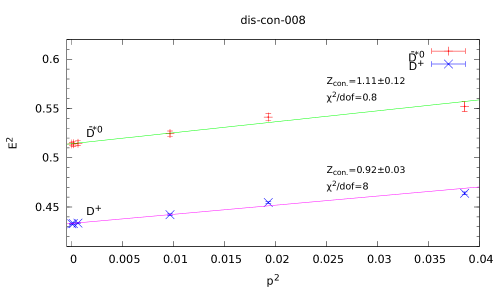
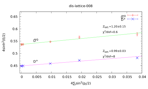
It is seen that the two dispersion relations yields compatible results which indicates that even for objects like charmed mesons, lattice artifacts are quite small. This is consistent with our previous experiences and might be due to one or several of the following reasons: the automatic $O(a)$ improvement of the twisted mass fermions, the smallness of our lattice spacing, and that we are studying low-energy scattering with small momenta.

Apart from the single-particle dispersion relations, it has also been suggested in previous lattice studies that it might be advantageous to also modify the two-particle dispersion relation in Eq. (2), see e.g. Refs. Lang et al. (2011); Mohler et al. (2013). We have also checked this possibility and found that, in our case, all $q^{2}$ values which eventually enter Lüscher’s formula (i.e. those values in Table  3) are consistent within errors with those obtained from the continuum dispersion relation, i.e. Eq. (2). We therefore simply take the values obtained from the continuum dispersion.

IV.1 Extraction of two-particle energy levels

To extract the two-particle energy eigenvalues, we adopt the usual Lüscher-Wolff method Lüscher and Wolff (1990). For this purpose, a new matrix $\Omega(t,t_{0})$ is defined as:

$$\Omega(t,t_{0})=C(t_{0})^{-{1\over 2}}C(t)C(t_{0})^{-{1\over 2}},$$ (28)

where $t_{0}$ is a reference time-slice. Normally one picks a $t_{0}$ such that the signal is good and stable. The energy eigenvalues for the two-particle system are then obtained by diagonalizing the matrix $\Omega(t,t_{0})$. The eigenvalues of the matrix have the usual exponential decay behavior as described by Eq. (24) and therefore the exact energy $E_{\alpha}$ can be extracted from the effective mass plateau of the eigenvalue $\lambda_{\alpha}$.

The real signal for the eigenvalue in our simulation turns out to be somewhat noisy. To enhance the signal, the following ratio was attempted:

$${\mathcal{R}}_{\alpha}(t,t_{0})={\lambda_{\alpha}(t,t_{0})\over C^{{\mathcal{V}}}(t-t_{0},{\bf 0})C^{{\mathcal{P}}}(t-t_{0},{\bf 0})}\propto e^{-\Delta E_{\alpha}\cdot(t-t_{0})}\;,$$ (29)

where $C^{{\mathcal{V}}}(t-t_{0},{\bf 0})$ and $C^{{\mathcal{P}}}(t-t_{0},{\bf 0})$ are one-particle correlation functions with zero momentum for the corresponding mesons defined in Eq. (III.3). Therefore, $\Delta E_{\alpha}$ is the difference of the two-particle energy measured from the threshold of the two mesons:

$$\Delta E_{\alpha}=E_{\alpha}-m_{D^{\ast}}-m_{D}\;.$$ (30)

The energy difference $\Delta E_{\alpha}$ can be extracted from the plateau behavior of the effective mass function $\Delta E_{\rm eff}(t)$ constructed from the ratio ${\mathcal{R}}_{\alpha}(t,t_{0})$ as usual. For all of the fits, the resulting $\chi^{2}$ per degree of freedom is around or less than one and the range is searched for by minimizing the $\chi^{2}$ per degree of freedom. The final results for $\Delta E_{\alpha}$, together with the corresponding ranges from which the $\Delta E_{\alpha}$’s are obtained, are summarized in Table 3. We only list the lowest two energy levels for the non-twisted case and the twisted cases of ${\mbox{\boldmath$\theta$}}=(0,0,\pi/8)$ and ${\mbox{\boldmath$\theta$}}=(0,0,\pi/4)$, since we are not going to use those higher energy levels to extract the scattering parameters in the following analysis.

Figure 2: Effective mass plots for the energy shift $\Delta E_{\alpha}$ at $\mu=0.003$ in the $A_{1}$ channel for ${\mbox{\boldmath$\theta$}}={\bf 0}$ (top), ${\mbox{\boldmath$\theta$}}=(0,0,\pi/8)$ (middle) and ${\mbox{\boldmath$\theta$}}=(0,0,\pi/4)$ (bottom). Two different colors indicate two lowest energy levels obtained from the variational calculation using $N=4$ (top) or $N=3$ (middle and bottom) different two-particle operators constructed using different ${\mathbf{k}}_{\alpha}$ as described in Eq. (19). The grey horizontal bars indicate the fitted values for $\Delta E_{\alpha}$’s and the fitting ranges.

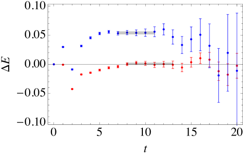
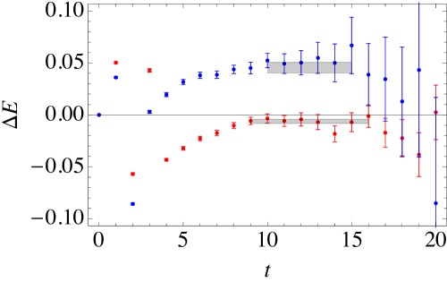
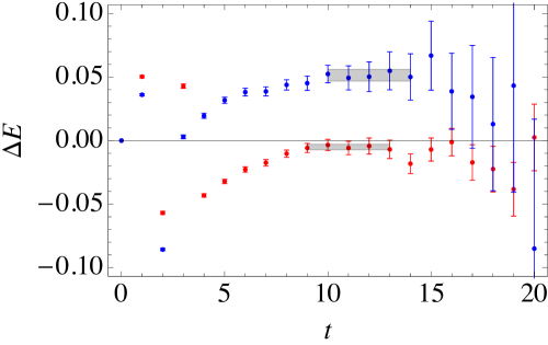
As an illustration, in Fig. 2, we have shown the effective mass plots and the fitted $\Delta E$’s at $\mu=0.003$ in the $A_{1}$ channel for three different values of $\theta$: ${\mbox{\boldmath$\theta$}}={\bf 0}$, ${\mbox{\boldmath$\theta$}}=(0,0,\pi/8)$ and ${\mbox{\boldmath$\theta$}}=(0,0,\pi/4)$. In these cases, we have chosen $N=3$ different two-particle operators and only the two lowest energy levels obtained from the (GEVP) process (23) are shown using red and blue points. Effective mass plots for other cases are similar. With the energy difference $\Delta E_{\alpha}$ extracted from the simulation data, one utilizes the definition:

$$\sqrt{m_{D^{\ast}}^{2}+\bar{\bf k}^{2}}+\sqrt{m_{D_{1}}^{2}+\bar{\bf k}^{2}}=\Delta E_{\alpha}+m_{D^{\ast}}+m_{D}\;.$$ (31)

to solve for $\bar{{\mathbf{k}}}^{2}\equiv(2\pi/L)^{2}q^{2}$ which is then plugged into Lüscher’s formula to obtain the information about the scattering phase shift.

$\theta$	Irrep	$\Delta E[t_{\min},t_{\max}](\mu=0.003)$		$\Delta E[t_{\min},t_{\max}](\mu=0.006)$		$\Delta E[t_{\min},t_{\max}](\mu=0.008)$
${\bf 0}$	$T_{1}$	0.001(1)[8,13]	0.054(2)[7,11]	-0.000(1)[10,14]	0.059(2)[7,11]	0.005(2)[13,17]	0.046(1)[7,11]
$(0,0,\frac{\pi}{8})$	$A_{1}$	-0.006(2)[9,16]	0.046(5)[10,15]	-0.005(2)[11,16]	0.051(2)[9,14]	0.005(4)[17,23]	0.056(4)[12,18]
	$E$	0.005(2)[10,15]	0.061(2)[6,11]	0.016(5)[18,23]	0.064(2)[9,14]	-0.002(1)[4,10]	0.061(4)[14,20]
$(0,0,\frac{\pi}{4})$	$A_{1}$	-0.005(2)[9,13]	0.051(5)[10,14]	-0.004(2)[11,16]	0.052(2)[9,14]	0.006(2)[13,20]	0.056(4)[12,18]
	$E$	0.005(2)[10,15]	0.061(2)[7,11]	0.022(8)[20,25]	0.065(2)[9,14]	-0.001(1)[4,12]	0.065(5)[14,20]
$(0,0,\pi)$	$A_{2}$	-0.015(5)[14,19]		0.014(7)[19,24]		0.021(5)[18,24]
	$E$	-0.003(10)[17,25]		0.043(9)[20,27]		0.028(6)[19,26]
$(\pi,\pi,0)$	$B_{1}$	0.003(10)[17,22]		0.026(6)[18,26]		0.059(8)[19,26]
	$B_{2}$	0.025(5)[12,17]		0.031(1)[6,12]		0.026(5)[16,22]
	$B_{3}$	0.029(1)[5,10]		0.020(4)[14,21]		0.029(1)[6,12]

Table 3: Results for the energy shifts $\Delta E$ obtained in our calculations for various cases. The time interval $[t_{\min},t_{\max}]$ from which we extract the values of $\Delta E$ are also listed. These ranges are relevant for the estimation of the error for the zeta functions as described in the text.

IV.2 Extraction of scattering information

It is well-known that, close to the scattering threshold, the quantity $k\cot\delta(k)$ has the following effective range expansion:

$${k^{2l+1}\cot\delta_{l}(k)}=a^{-1}_{l}+{1\over 2}r_{l}k^{2}+\cdots\;,$$ (32)

where $a_{l}$ is the so-called scattering length, $r_{l}$ is the effective range for partial wave $l$ while $\cdots$ represents terms that are higher order in $k^{2}$. We will call $a_{l}$ and $r_{l}$ the low-energy scattering parameters in the following. It is more convenient to express this formulae in terms of $q^{2}$:

$${q^{2l+1}\cot\delta_{l}(q^{2})}=B_{l}+{1\over 2}R_{l}q^{2}+\cdots\;,$$ (33)

with $B_{l}=[L/(2\pi)]^{2l+1}a^{-1}_{l}$ and $R_{l}=[L/(2\pi)]^{2l-1}r_{l}$. Our task is to extract the parameters $B_{l}$ and $R_{l}$ from the simulation data.

It is also well-known that, close to the threshold, scattering is dominated by phase shifts coming from lower partial waves as long as they are non-vanishing. We therefore will ignore all $l\geq 2$ partial waves in the Lüscher formula for this study. Thus to extract these low-energy scattering parameters from the lattice data, we have to distinguish two different scenarios: the parity-conserving scenario, which corresponds to the non-twisting case and twisting case with special angles (i.e. those with $\theta=\pi$), and the parity-mixing scenario (those with values of $\theta\neq 0$ or $\pi$). Accordingly, the values of $q^{2}$ obtained are also categorized into two classes: the parity-conserving case and the parity-mixing case. The number of data points (i.e. number of $q^{2}$ values) in the two case is denoted as $N_{0}$ and $N_{1}$, respectively. So altogether we have $N_{0}+N_{1}$ points for $q^{2}$ values which are exactly those listed in Table 3.

The major difference between the parity-conserving data and parity-mixing data is as follows. As we have neglected all contributions from $l\geq 2$ partial waves, the parity-conserving data is only relevant for the $s$-wave scattering parameters $B_{0}$ and $R_{0}$ while parity-mixing data is relevant for both $s$-wave and $p$-wave scattering parameters: $B_{0}$, $R_{0}$, $B_{1}$ and $R_{1}$. In previous studies like Ref. Ozaki and Sasaki (2013), the authors first used only the parity-conserving data to extract the $s$-wave scattering parameters. Then, the obtained scattering information for the $s$-wave is substituted into the fit for the $p$-wave parameters using the parity-mixing data. In this study, we attempt to simultaneously fit for all scattering parameters, both $s$-wave and $p$-wave, from all of our data points (both parity-conserving and parity-mixing).

Just to make comparisons, we have attempted the following methods for the extraction of the scattering parameters: we could use only the parity-conserving data ($N_{0}$ data points) or all of our data ($N_{0}+N_{1}$ data points). In either of these cases, we could perform either the correlated fit or the uncorrelated fit. The detailed process will be described below with the correlated fit using all data as an example, which is more involved than other methods and yields the most reliable results. We regard these as our final results in this paper. However, for comparison purposes, the results for other cases are also tabulated for reference in Table 4 and Table 5.

To be specific, in the parity-conserving case, we define

$$y_{0}(q^{2})=q\cot\delta_{0}(q^{2})\;.$$ (34)

According to Lüscher’s formula (4), this should be equal to

$$m_{00}(q^{2})={1\over\pi^{3/2}}{\mathcal{Z}}_{00}(1;q^{2})\;,$$ (35)

for the non-twisted case while for the twisted case of ${\mbox{\boldmath$\theta$}}=(0,0,\pi)$ and ${\mbox{\boldmath$\theta$}}=(\pi,\pi,0)$ one simply replace the corresponding zeta function by ${\mathcal{Z}}^{{\mbox{\boldmath$\theta$}}}_{00}(1;q^{2})$. In the parity-mixing case, however, things are more complicated. Apart from the $s$-wave phase shift $\delta_{0}(q^{2})$, Lüscher formula will also involve $\delta_{1}(q^{2})$ and maybe written as Eq. (11). We therefore define

$$y_{1}(q^{2})=\left[q\cot\delta_{0}-m_{00}\right]\left[q^{3}\cot\delta_{1}-m_{11}\right]\;.$$ (36)

which, according to Lüscher formula, should be equal to $m^{2}_{01}(q^{2})$. Note that in either case, the functions $m_{00}$, $m_{01}$, $m_{11}$ are all known functions of $q^{2}$ that involve various zeta-functions Ozaki and Sasaki (2013). In the following, these functions will be generally denoted as $Z(q^{2})$ for convenience. In other words, $Z(q^{2})$ stands for $m_{00}(q^{2})$ and $m^{2}_{01}(q^{2})$ in the parity-conserving and parity-mixing case, respectively.

One subtlety that concerns us is the estimation of errors for $Z(q^{2})$ which are rapidly oscillating functions of $q^{2}$. These functions can also become divergent at specific values. The naive way of estimating the errors would be for each $q^{2}_{I}$ value and its error $\Delta q^{2}_{I}$, one simply substitutes $Z(q^{2}_{I})$ for the central value and using $Z(q^{2}_{I}\pm\Delta q^{2}_{I})$ for the estimation of the error. This is fine for some of our $q^{2}$ values but for $q^{2}$ values that are close to the divergent points of these functions, this results in extraordinarily large (and asymmetric) errors. We therefore attempted to estimate the errors for these functions directly from the data using the jack-knife method.

To do this, recall that our values of $q^{2}_{I}$, with $I=1,\cdots,N_{0}+N_{1}$, are obtained from the corresponding energy shifts $\delta E_{\alpha}$ as described in the previous section and then using Eq. (31) to convert into values of $\bar{{\mathbf{k}}}^{2}$, or equivalently, $q^{2}$. In this process, we have obtained a set of jack-knifed, (Euclidean) time-dependent values for $q^{2}$: $q^{2}_{I,a}(t)$, where $t$ denotes the time slice and $a$ indicates the corresponding value with the configuration numbered by $a$ left out. By searching an appropriate plateau in $t\in[t_{\min},t_{\max}]$, say by minimizing the $\chi^{2}$ per degree of freedom, we have obtained the values of $q^{2}_{I}$ using all of our configurations. These $q^{2}_{I}$ values are equivalent to the values of $\Delta E$ listed in Table 3 with the help of Eq. (31). The corresponding ranges $[t_{\min},t_{\max}]$ are also tabulated in Table 3. Within the same temporal ranges that determine various values of $q^{2}_{I}$, we could define a (Euclidean) time-dependent zeta-function using the jack-knifed data sets $q^{2}_{I,a}(t)$ via

$$Y^{a}_{I}(t)=Z(q^{2}_{I,a}(t))\;,\;\;t\in[t_{\min},t_{\max}]\;.$$ (37)

and also its average value:

$$\bar{Y}_{I}(t)={1\over N}\sum^{N}_{a=1}Y^{a}_{I}(t)\;.$$ (38)

We then estimate the errors of $\bar{Y}_{I}(t)$ using conventional jackknife:

$$\Delta Y_{I}(t)=\sqrt{{N-1\over N}\sum^{N}_{a=1}[Y^{a}_{I}(t)-\bar{Y}_{I}(t)]^{2}}\;.$$ (39)

In the next step, we define the weighted-average $Y^{a}_{I}$ over the temporal slices:

$$Y^{a}_{I}=\sum_{t}p_{I}(t)Y^{a}_{I}(t)\;,$$ (40)

with the probability $p(t)$ for time slice $t$ given by

$$p_{I}(t)={[\Delta Y_{I}(t)]^{-2}\over\sum_{t}[\Delta Y_{I}(t)]^{-2}}\;,$$ (41)

where the summation is within the corresponding range of $[t_{\min},t_{\max}]$ for that particular $q^{2}_{I}$. Note that the weighted average $Y^{a}_{I}$ in Eq. (40) is equivalent to searching the plateau of $Y^{a}_{I}(t)$ in $t$, except that we demand that the range of this average should coincide with the range that we determined for the corresponding $q^{2}$ value. We can then define the expectation value

$$\bar{Y}_{I}={1\over N}\sum_{a}Y^{a}_{I}\;,$$ (42)

and the corresponding covariance matrix,

$$C_{IJ}={N-1\over N}\sum_{a}(Y^{a}_{I}-\bar{Y}_{I})(Y^{a}_{J}-\bar{Y}_{J})\;.$$ (43)

Thus, $C$ is an $(N_{0}+N_{1})\times(N_{0}+N_{1})$ matrix which incorporates also the correlations among $y_{0}$’s and $y_{1}$’s. This covariance matrix is estimated using our data sample and the corresponding inverse matrix $C^{-1}$ can also be obtained numerically. We stress that, though in some cases the matrix has rather large condition number (see below for further discussion), we had no practical problem in obtaining $C^{-1}$ using the standard methods.

For later convenience, we introduce an index function as follows,

$$ind(I)=\left\{\begin{aligned} 0\;\;&\mbox{for $1\leq I\leq N_{0}$}\\ 1\;\;&\mbox{for $N_{0}+1\leq I\leq N_{0}+N_{1}$}\end{aligned}\right.$$ (44)

In other words, $ind(I)=0$ for the first $N_{0}$ parity-conserving data points while $ind(I)=1$ for the next $N_{1}$ parity-mixing data points. So our previous definitions of $y_{0}(q^{2})$ and $y_{1}(q^{2})$ may be written collectively as $y_{ind(I)}(q^{2}_{I})$ with $I=1,2,\cdots,(N_{0}+N_{1})$.

Figure 3: Results for the correlated fits as described in the text. Each panel, from top to bottom, corresponds to $\mu=0.003,0.006$ and $0.008$, respectively. The quantity $q\cot\delta_{0}(q^{2})$ is plotted versus $q^{2}$ for all our data points, both parity-conserving (blue) case and parity-mixing case (green). The straight lines and the bands indicate the fitted result for $F_{0}(q^{2})=B_{0}+(R_{0}/2)q^{2}$ and the corresponding uncertainties in $B_{0}$ and $R_{0}$.

Finally, we can construct the $\chi^{2}$ function as usual

$$\chi^{2}=\sum^{N_{0}+N_{1}}_{I,J=1}\left[F_{ind(I)}(q^{2}_{I};\alpha)-y_{ind(I)}(q^{2}_{I})\right]C^{-1}_{IJ}\left[F_{ind(J)}(q^{2}_{J};\alpha)-y_{ind(J)}(q^{2}_{J})\right]\;.$$ (45)

where for $ind(I)=0,1$ the corresponding functions are (using the symbol $\alpha$ to collectively denote all the relevant parameters $B_{0}$, $R_{0}$, $B_{1}$ and $R_{1}$):

$$\!\!\!\!\!\!F_{0}(q^{2};\alpha)=B_{0}+{1\over 2}R_{0}q^{2}\;,$$ (46)

$$\!\!\!\!\!\!F_{1}(q^{2};\alpha)=[B_{0}+{R_{0}\over 2}q^{2}-m_{00}][B_{1}+{R_{1}\over 2}q^{2}-m_{11}].$$ (47)

Minimizing the target $\chi^{2}$ function in Eq. (45), one could obtain all the parameters, namely $B_{0}$, $R_{0}$, $B_{1}$ and $R_{1}$, in a single step with all of our data. This completes the process of correlated fit using all of our data.

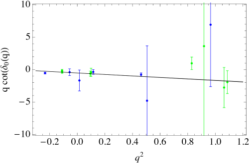
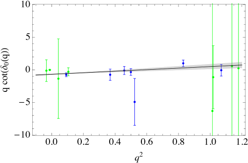
To get a feeling of the quality of the fits, we plot the quantity $q\cot\delta_{0}(q^{2})$ vs. $q^{2}$ in Fig. 3. This figure illustrates the situation for all three pion masses in our simulation. From top to bottom, each panel corresponds to $\mu=0.003$, $\mu=0.006$ and $\mu=0.008$, respectively. The data points obtained from our simulation are also plotted in these figures. The blue points are the data points from the parity-conserving case while the green points are the data for the parity-mixing case. For the former case, the errors for the data points are estimated using jack-knife method, i.e. the diagonal matrix element of the covariance matrix. In the latter case, the values of $q\cot\delta_{0}(q^{2})$ are obtained via the relation

$$q\cot\delta_{0}=m_{00}+{m^{2}_{01}\over q^{3}\cot\delta_{1}(q^{2})-m_{11}}\;,$$ (48)

where the quantity $q^{3}\cot\delta_{1}(q^{2})$ on the r.h.s of the equation is replaced by $B_{1}+(R_{1}/2)q^{2}$ with the fitted values for $B_{1}$ and $R_{1}$. The errors for these points are estimated by the jack-knife method using the r.h.s. of the above equation. The straight lines and the grey shaded bands in the figure illustrates the function $F_{0}(q^{2};\alpha)=B_{0}+(R_{0}/2)q^{2}$ and the uncertainties in the parameter ($B_{0}$ and $R_{0}$), respectively. As is seen from the figure, we get a reasonable fit for all three pion mass values.

Figure 4: The quantity $q^{3}\cot\delta_{1}(q^{2})$ vs. $q^{2}$ for the parity-mixing data at $\mu=0.003$.

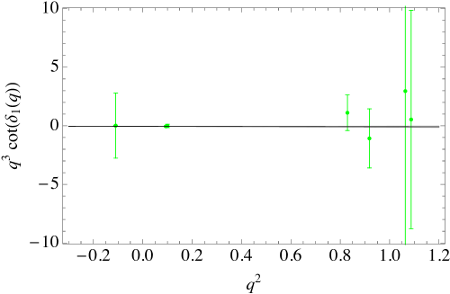
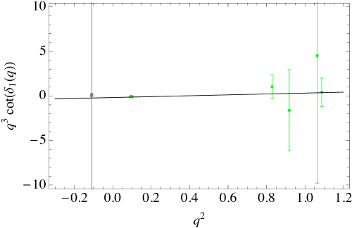
In a similar fashion, we could also plot the quantity $q^{3}\cot\delta_{1}(q^{2})$ vs. $q^{2}$ for the parity-mixing data. This is shown in Fig. 4 for $\mu=0.003$ as an example.

Note that, as far as the $s$-wave scattering parameters $B_{0}$ and $R_{0}$ are concerned, although they are most directly derived from the parity-conserving points (i.e. the blue points in Fig. 3), the parity-mixing points (the green points in Fig. 3) also help to reduce the uncertainties in these parameters substantially. The effects coming from these points are folded in through the covariance matrix defined in Eq. (43). To see this effect, one has to compare these results with the results obtained without the parity-mixing points. With the results listed in Table 4 and Table 5, it is seen that the parity-mixing points do indeed help to reduce the uncertainties in $B_{0}$ and $B_{1}$ in most cases.

		$B_{0}$	$R_{0}$	$B_{1}$	$R_{1}$	$\chi^{2}/dof$
003	Uncorrelated	-0.50(0.02)	-2.1(0.3)	-0.02(0.01)	-0.5(0.2)	39.8/11
	Correlated	-0.513(0.008)	-2.3(0.1)	-0.047(0.006)	-0.1(0.2)	47.0/11
	Correlated (omitted)	-0.35(0.12)	0.8(0.6)	-0.17(0.04)	1.00(0.09)	24.7/8
006	Uncorrelated	-0.176(0.005)	-1.1(0.1)	0.4(0.1)	-3.1(0.5)	15.8/11
	Correlated	-0.16(0.01)	-0.8(0.2)	0.29(0.05)	-2.6(0.3)	28.1/ 11
	Correlated (omitted)	0.6(0.3)	-3.8(1.6)	-9.3(2.3)	17.8(5.0)	7.8/ 8
008	Uncorrelated	-0.6(0.1)	1.8(0.7)	-0.02(0.01)	0.4(0.5)	9.6/11
	Correlated	-0.67(0.09)	2.4(0.8)	-0.037(0.008)	-0.1(0.2)	17.0/11
	Correlated (omitted)	-0.71(0.08)	2.3(0.7)	0.02(0.03)	-0.2(0.2)	13.5/9

Table 4: Fit results with parity-conserving and parity-mixing points.

		$B_{0}$	$R_{0}$	$\chi^{2}/dof$
003	Uncorrelated	-0.6(0.1)	-0.5(0.8)	2.1/5
	Correlated	-0.6(0.1)	-0.6(0.8)	2.7/5
006	Uncorrelated	0.6(0.7)	-4.2(2.1)	6.4/5
	Correlated	1.0(0.7)	-4.5(1.8)	6.5/ 5
008	Uncorrelated	-0.9(0.3)	3.4(1.2)	4.6/5
	Correlated	-0.8(0.3)	3.8(1.1)	5.5/5

Table 5: Fit results with parity-conserving data only.

Figure 5: The same as Fig. 3 except that the grey data points are omitted in the $\chi^{2}$ fitting process for stability reasons as explained in the text.

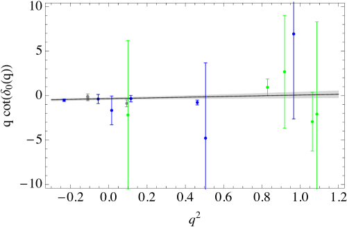
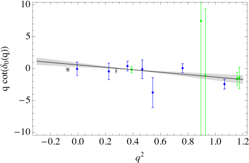
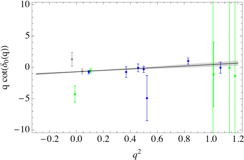
In the course of inverting the covariance matrix $C$, it is found that in some cases the matrix is close to singular. This might bring up some potential worry about the stability of the fits. We studied this situation using the singular value decomposition method. We found that this close to singularity was caused by some of our $q^{2}$ values in some of the irreps in our calculation. To be specific, these correspond mainly to the lowest energy levels in irrep $A_{1}$ and $E$ at ${\mbox{\boldmath$\theta$}}=(0,0,\pi/8)$ from the parity-mixing data. Therefore, we have attempted the same fits as before except that with these data points omitted in the $\chi^{2}$ fitting process. This results in omitting $3$, $3$ and $2$ data points from $\mu=0.003$, $0.006$ and $0.008$, respectively. There is no well-established cut as to which points should be neglected in general but this procedure helps to give us some idea when compared with the results obtained with all the data. However, just to offer an idea where these omitted data points actually go, they are still plotted in the Fig. 5 and Fig. 6 using grey data points. It is seen that the $B_{0}$ results for $\mu=0.003$ and $\mu=0.008$ do not change much except that the errors are larger. For $\mu=0.006$, the central values of $B_{0}$ and $R_{0}$ changed substantially with the corresponding errors are also much larger. For example, the estimate of $B_{0}$ changes from $-0.16(1)$ to $0.6(3)$, making the original value some $2.5\sigma$ below the new value. This is understandable from the middle panel in Fig. 5 where it is clearly seen that the three grey data points (the omitted ones) all lie significantly below the fitted straight line. This result is in fact in accordance with (consistent within errors) the results using only the parity-conserving data as listed in Table 5. Since there are no good reasons why these data points should be neglected in the first place and that they result in much larger errors, we think our original fits with all the data being more reasonable. However, the results with grey data points neglected are also tabulated for comparison.

Figure 6: The same as Fig. 4 except that the grey data points are omitted in the fit.

The fitted values for the scattering parameters are summarized in Table 4 for three values of $m^{2}_{\pi}$ in our simulation. As is said, we have performed both the correlated fits and uncorrelated fits. In the case of uncorrelated fits, we do not construct the covariance matrix as in Eq. (43). We simply estimate the diagonal matrix elements $[\Delta Y_{I}]^{-2}$ using the conventional jackknife method. In the same table, under the title “correlated (omitted)” for each parameter $\mu$, we have also listed the results with the grey data points omitted in the $\chi^{2}$ fitting process as explained above. Finally, we could also do our fits using only the parity-conserving data, as is done in previous studies Ozaki and Sasaki (2013). The results for the $s$-wave scattering parameters are listed in Table 5 for comparison. As the correlation among different $Y_{I}$’s are quite substantial, especially those among $y_{0}$’s and $y_{1}$’s, as we observed from our covariance matrices, we regard our correlated fits with all of our data as being more reliable and they are taken as our final results.

IV.3 Physical values for the scattering parameters

It is straightforward to convert the fitted values of $B_{0}$, $R_{0}$, $B_{1}$ and $R_{1}$ obtained in the previous subsection into physical units using the relation

$$a_{l}=\left({L\over 2\pi}\right)^{2l+1}\left({1\over B_{l}}\right)\;,\;\;r_{l}=R_{l}\left({2\pi\over L}\right)^{2l-1}\;.$$ (49)

Then, if we take the numbers in Table 4, we get for the $s$-wave scattering length $a_{0}$: $-0.67(1)$fm, $-2.13(13)$fm, $-0.51(7)$fm for $\mu=0.003$, $0.006$, $0.008$, respectively. The values for $r_{0}$ are also obtained accordingly. These numbers are summarized in Table. 6

It is observed that the values we get for $a_{0}$ do not seem to follow a simple regular chiral extrapolation within the range that we have studied. We therefore kept the individual values for $a_{0}$ and $r_{0}$ for each case. This irregularity might be caused by the smallness of the value $m_{\pi}L\sim 3.3$ for $\mu=0.003$. To circumvent this, one has to study a larger lattice.

The negative values of the parameter $B_{0}$ (hence the scattering length $a_{0}$) indicates that the two constituent mesons for the $(D\bar{D}^{*})^{\pm}$ system have weak repulsive interactions at low energies. Therefore, our result does not support the bound state scenario for these two mesons. Recall that for an infinitely shallow bound state, we should have $B_{0}\sim 0^{+}$ but our values of $B_{0}$ are all negative for all three pion mass values, as can be seen from Table 4 and Table 5. The exceptions are the $\mu=0.006$ data sample using only the parity-conserving data or the correlated fit using all data but with three data points omitted. All these contradicts the possibility of a bound state, at least for the pion mass values we studied.

	$\mu=0.003$	$\mu=0.006$	$\mu=0.008$
$a_{0}$[fm]	-0.67(1)	-2.1(1)	-0.51(7)
$r_{0}$[fm]	-0.78(3)	-0.27(7)	0.82(27)

Table 6: The values for $a_{0}$ and $r_{0}$ in physical units obtained from the numbers for the correlated fit in Table 4.

Another check for the possible bound state would be to look for those negative $q^{2}$ values we obtained which corresponds to the negative values of $\delta E$ listed in Table 3. However, one has to keep in mind that a negative value of $q^{2}$ does not necessarily signal a bound state in the infinite volume limit. Instead, for a finite volume, one has to check the condition in Eq. (6). The second term on the r.h.s of this equation indicates the size of the finite volume correction. This correction has to be small enough to justify the usage of this criterion since other higher order terms are neglected. We have checked all our data points with negative $q^{2}$ and they do not seem to satisfy this condition. Therefore, our conclusion is that there is no indication of a bound state in this channel below the threshold, as far as we can tell from our data. This conclusion is consistent with a recent lattice study using Wilson fermions Prelovsek et al. (2013). Since the cases we are studying is still far from the physical pion mass case, we therefore still cannot rule out the possibility the appearance of a bound state once the pion mass is lowered (and the lattice size $L$ is also increased accordingly to control the finite volume corrections). Such scenarios do occur in lattice studies of two nucleons.

V Conclusions

In this paper, we present an exploratory lattice study for the low-energy scattering of $(D\bar{D}^{*})^{\pm}$ two meson system near the threshold using single-channel Lüscher’s finite-size technique. The calculation was based on $N_{f}=2$ twisted mass fermion configurations of size $32^{3}\times 64$ with a lattice spacing of about $0.067$fm. To investigate the pion mass dependence, three pion mass values are studied which corresponds to $m_{\pi}=300$MeV, 420MeV and 485MeV, respectively. To enhance the momentum resolution close to the threshold, twisted boundary conditions are also utilized together with the conventional periodic boundary conditions. Twisted boundary conditions also causes the mixing of $p$-wave with the $s$-wave scattering phase due to reduced symmetry. We have performed a combined analysis, using both the parity-conserving data and the parity-mixing data to obtain the scattering parameters. Our study mainly focuses on the $s$-wave scattering in the channel $J^{P}=1^{+}$ and the scattering threshold parameters, i.e. scattering length $a_{0}$ and effective range $r_{0}$ are obtained. An estimate for the $p$-wave scattering parameters are also obtained as a by-product.

Our result indicates that the scattering lengths are negative, indicating a weak repulsive interaction between the the two mesons ($D$ and $\bar{D}^{*}$ or its conjugated systems under $C$-parity or $G$-parity). This is true for all three pion mass values that we simulated. We have also checked the possibility of the bound state for those negative energy shifts. None of those is consistent with a bound state. Our conclusion is that, based on our current lattice result, we do not support a bound state in this channel. Similar conclusion has been reached in a recent lattice study using Wilson fermions on a smaller lattice Prelovsek and Leskovec (2013a); Prelovsek et al. (2013). However, as we pointed out already, we cannot rule out the possible appearance of a bound state for the two charmed mesons if the pion mass is lowered and the volume is increased accordingly. This requires further more systematic lattice studies. Furthermore, it is also possible the the quantum numbers of the observed $Z_{c}(3900)$ is not $1^{+}$ or more complete set of interpolation operators and a coupled channel study is required. Thus, this lattice study has shed some light on the nature of $Z^{\pm}_{c}(3900)$ however it remains to be clarified by future studies.

References

- Ablikim et al. (2013) M. Ablikim et al. (BESIII Collaboration), Phys.Rev.Lett. 110, 252001 (2013), arXiv:1303.5949 [hep-ex] .
- Liu et al. (2013) Z. Liu et al. (Belle Collaboration), Phys.Rev.Lett. 110, 252002 (2013), arXiv:1304.0121 [hep-ex] .
- Xiao et al. (2013) T. Xiao, S. Dobbs, A. Tomaradze, and K. K. Seth, Phys.Lett. B727, 366 (2013), arXiv:1304.3036 [hep-ex] .
- Wang et al. (2013) Q. Wang, C. Hanhart, and Q. Zhao, Phys.Rev.Lett. 111, 132003 (2013), arXiv:1303.6355 [hep-ph] .
- Lüscher (1986a) M. Lüscher, Commun. Math. Phys. 104, 177 (1986a).
- Lüscher (1986b) M. Lüscher, Commun. Math. Phys. 105, 153 (1986b).
- Lüscher and Wolff (1990) M. Lüscher and U. Wolff, Nucl. Phys. B 339, 222 (1990).
- Lüscher (1991a) M. Lüscher, Nucl. Phys. B 354, 531 (1991a).
- Lüscher (1991b) M. Lüscher, Nucl. Phys. B 364, 237 (1991b).
- Prelovsek and Leskovec (2013a) S. Prelovsek and L. Leskovec, Phys.Lett. B727, 172 (2013a), arXiv:1308.2097 [hep-lat] .
- Prelovsek et al. (2013) S. Prelovsek, L. Leskovec, and D. Mohler, (2013), arXiv:1310.8127 [hep-lat] .
- Prelovsek and Leskovec (2013b) S. Prelovsek and L. Leskovec, Phys.Rev.Lett. 111, 192001 (2013b), arXiv:1307.5172 [hep-lat] .
- Sasaki and Yamazaki (2006) S. Sasaki and T. Yamazaki, Phys.Rev. D74, 114507 (2006), arXiv:hep-lat/0610081 [hep-lat] .
- Bedaque (2004) P. F. Bedaque, Phys.Lett. B593, 82 (2004), arXiv:nucl-th/0402051 [nucl-th] .
- Sachrajda and Villadoro (2005) C. Sachrajda and G. Villadoro, Phys.Lett. B609, 73 (2005), arXiv:hep-lat/0411033 [hep-lat] .
- Ozaki and Sasaki (2013) S. Ozaki and S. Sasaki, Phys.Rev. D87, 014506 (2013), arXiv:1211.5512 [hep-lat] .
- Agadjanov et al. (2014) D. Agadjanov, U.-G. Meissner, and A. Rusetsky, JHEP 1401, 103 (2014), arXiv:1310.7183 [hep-lat] .
- Meng et al. (2009) G.-Z. Meng et al. (CLQCD Collaboration), Phys.Rev. D80, 034503 (2009), arXiv:0905.0752 [hep-lat] .
- Liu et al. (2008) Y.-R. Liu, X. Liu, W.-Z. Deng, and S.-L. Zhu, Eur.Phys.J. C56, 63 (2008), arXiv:0801.3540 [hep-ph] .
- Ablikim et al. (2014) M. Ablikim et al. (BESIII Collaboration), Phys.Rev.Lett. 112, 022001 (2014), arXiv:1310.1163 [hep-ex] .
- Song He (2005) C. L. Song He, Xu Feng, JHEP 0507, 011 (2005).
- Liu et al. (2006) C. Liu, X. Feng, and S. He, Int.J.Mod.Phys. A21, 847 (2006), arXiv:hep-lat/0508022 [hep-lat] .
- Lage et al. (2009) M. Lage, U.-G. Meißner, and A. Rusetsky, Phys.Lett. B681, 439 (2009), arXiv:0905.0069 [hep-lat] .
- Bernard et al. (2011) V. Bernard, M. Lage, U.-G. Meißner, and A. Rusetsky, JHEP 1101, 019 (2011), arXiv:1010.6018 [hep-lat] .
- Döring et al. (2011) M. Döring, U.-G. Meißner, E. Oset, and A. Rusetsky, Eur.Phys.J. A47, 139 (2011), arXiv:1107.3988 [hep-lat] .
- Döring et al. (2012) M. Döring, U. Meißner, E. Oset, and A. Rusetsky, Eur.Phys.J. A48, 114 (2012), arXiv:1205.4838 [hep-lat] .
- Li et al. (2014) N. Li et al., (2014), work in progress.
- Frezzotti and Rossi (2004) R. Frezzotti and G. Rossi, JHEP 0410, 070 (2004), arXiv:hep-lat/0407002 [hep-lat] .
- Lang et al. (2011) C. Lang, D. Mohler, S. Prelovsek, and M. Vidmar, Phys.Rev. D84, 054503 (2011), arXiv:1105.5636 [hep-lat] .
- Mohler et al. (2013) D. Mohler, S. Prelovsek, and R. Woloshyn, Phys.Rev. D87, 034501 (2013), arXiv:1208.4059 [hep-lat] .