Hidden-charm and bottom meson-baryon molecules coupled with five-quark states

Abstract

In this paper, we investigate the hidden-charm pentaquarks as $\bar{D}^{(\ast)}\Lambda_{\rm c}$ and $\bar{D}^{(\ast)}\Sigma^{(\ast)}_{\rm c}$ molecules coupled to the five-quark states. Furthermore, we extend our calculations to the hidden-bottom sector. The coupling to the five-quark states is treated as the short range potential, where the relative strength for the meson-baryon channels is determined by the structure of the five-quark states. We found that resonant and/or bound states appear in both the charm and bottom sectors. The five-quark state potential turned out to be attractive and, for this reason, it plays an important role to produce these states. In the charm sector, we need the five-quark potential in addition to the pion exchange potential in producing bound and resonant states, whereas, in the bottom sector, the pion exchange interaction is strong enough to produce states. Thus, from this investigation, it emerges that the hidden-bottom pentaquarks are more likely to form than their hidden-charm counterparts; for this reason, we suggest that the experimentalists should look for states in the bottom sector.

I Introduction

The study of the exotic hadrons has aroused great interest in nuclear and hadron physics. In 2015, the Large Hadron Collider beauty experiment (LHCb) collaboration observed two hidden-charm pentaquarks, $P^{+}_{c}(4380)$ and $P^{+}_{c}(4450)$, in $\Lambda^{0}_{b}\rightarrow J/\psi K^{-}p$ decay Aaij:2015tga ; Aaij:2016phn ; Aaij:2016ymb . These two pentaquark states are found to have masses of $4380\pm 8\pm 28\;$ MeV and $4449.8\pm 1.7\pm 2.5\;$ MeV, with corresponding widths of $205\pm 18\pm 86\;$ MeV and $39\pm 5\pm 19\;$ MeV. The spin-parity $J^{P}$ of these states has not yet been determined. The parities of these states are preferred to be opposite, and one state has $J=3/2$ and the other $J=5/2$. $(J^{P}_{P^{+}_{c}(4380)},J^{P}_{P^{+}_{c}(4450)})=(3/2^{-},5/2^{+})$ gives the best fit solution, but $(3/2^{+},5/2^{-})$ and $(5/2^{-},3/2^{+})$ are also acceptable. The $P^{+}_{\rm c}$ resonances are one of topics of great interest as the candidates of the exotic multiquark state, and many discussions have been done so far Chen:2016qju ; Ali:2017jda ; Esposito:2016noz .

Hidden-charm pentaquark states, such as $uudc\bar{c}$ and $udsc\bar{c}$ compact structures, have been studied so far. Before $P^{+}_{\rm c}$ observed by LHCb, Yuan et al. in Yuan:2012wz studied the $uudc\bar{c}$ and $udsc\bar{c}$ systems by the non-relativistic harmonic oscillator Hamiltonian with three kinds of the schematic interactions: a chromomagnetic interaction, a flavor-spin-dependent interaction and an instanton-induced interaction. In Santopinto:2016pkp , Santopinto et al. investigated the hidden-charm pentaquark states as five-quark compact states in the $S-$wave by using a constituent quark model approach. The hidden-charm and hidden-bottom pentaquark masses have been calculated by Wu et al. in Wu:2017weo , by means of a color-magnetic interaction between the three light quarks and the $c\bar{c}$ ($b\bar{b}$) pair in a color octet state. Takeuchi et al. Takeuchi:2016ejt has also investigated the hidden-charm pentaquark states by the quark cluster model, and discussed the structure of the five-quark states which appears in the scattering states. To investigate the compact five-quark state, the diquark model has also been applied Maiani:2015vwa ; Li:2015gta ; Ali:2016dkf ; Lebed:2015tna ; Zhu:2015bba ; Zhu:2015bba . The quantum chromodynamics (QCD) sum rules with the diquark picture were applied in Refs. Wang:2015epa ; Wang:2015ava . However, these authors do not provide any information about the pentaquark widths. Despite many theoretical works and implications, there is so far no clear evidence of such compact multiquark states.

By contrast, it is widely accepted that there are candidates for hadronic molecular states. A long-standing and well-known example is $\Lambda(1405)$, which is considered to be a molecule of $\bar{K}N$ and $\pi\Sigma$ coupled channels. A general review of $\Lambda(1405)$ can be found in Hyodo:2011ur . In the heavy quark sector, $X(3872)$ Choi:2003ue , $Z_{b}(10610)$, and $Z_{b}(10650)$ Collaboration:2011gja are considered to be, respectively, $D\bar{D}^{\ast}$ Tornqvist:2004qy ; Close:2003sg ; Braaten:2003he ; Wong:2003xk ; Swanson:2003tb ; Swanson:2004pp and $B^{(\ast)}\bar{B}^{\ast}$ molecules Bondar:2011ev ; Ohkoda:2011vj . Now, the $P^{+}_{c}$ pentaquarks have been found just below the $\bar{D}\Sigma^{\ast}_{\rm c}$ and $\bar{D}^{\ast}\Sigma_{\rm c}$ thresholds. Thus, the $\bar{D}\Sigma^{\ast}_{\rm c}$ and $\bar{D}^{\ast}\Sigma_{\rm c}$ molecular components are expected to be dominant Wu:2010jy ; Wu:2010vk ; Garcia-Recio:2013gaa ; Karliner:2015ina ; Chen:2015loa ; Roca:2015dva ; He:2015cea ; Meissner:2015mza ; Chen:2015moa ; Uchino:2015uha ; Burns:2015dwa ; Shimizu:2016rrd ; Yamaguchi:2016ote ; Shimizu:2017xrg . Moreover, the baryocharmonium structure as the composite of $J/\psi$ and the excited nucleon $N^{\ast}$ is also discussed Kubarovsky:2015aaa .

In the formation of the hadronic molecules, the one pion exchange potential (OPEP) would be a key ingredient to bind the composite hadrons. In nuclear physics, it has been well-known that the pion-exchange is a driving force to bind atomic nuclei Ikeda:2010aq . Moreover, it was also applied to the deuteronlike bound states of two hadrons, which is called deusons Tornqvist:1993ng . Specifically in the heavy quark sector, the role of the pion-exchange would be enhanced by the heavy quark spin symmetry. The important property of this symmetry is that in the heavy quark mass limit, the spin of heavy (anti)quarks, $s_{Q}$, is decoupled from the total angular momentum of the light degrees of freedom, $j$, which is carried by light quarks and gluons Isgur:1989vq ; Isgur:1989ed ; Isgur:1991wq ; Neubert:1993mb ; Manohar:2000dt ; Yasui:2013vca ; Yamaguchi:2014era ; Hosaka:2016ypm . Thus, the heavy quark spin (HQS) multiplet emerges, where hadrons in the multiplet have the same mass, even though the hadrons have different total angular momenta given by $s_{Q}\otimes j$. In the charm (bottom) mesons, a $\bar{D}$ ($B$) meson as a pseudoscalar meson is regarded as the member of the HQS doublet whose pair is a $\bar{D}^{\ast}$ ($B^{\ast}$) meson as a vector meson. In fact, the mass difference of $\bar{D}$ and $\bar{D}^{\ast}$ mesons ($B$ and $B^{\ast}$ mesons) is small, $m_{\bar{D}^{\ast}}-m_{\bar{D}}\sim 140$ MeV ($m_{B^{\ast}}-m_{B}\sim 45$ MeV). In contrast, the mass differences in the light flavor sectors are given by $m_{\rho}-m_{\pi}\sim 630$ MeV and $m_{K^{\ast}}-m_{K}\sim 390$ MeV. The approximate mass degeneracy enhances the attraction due to the mixing of the $\bar{D}$ ($B$) meson and the $\bar{D}^{\ast}$ ($B^{\ast}$) meson caused by the pion-exchange. We note that the heavy meson is coupled to the pion through the $\bar{D}^{\ast}\bar{D}\pi$ and $\bar{D}^{\ast}\bar{D}^{\ast}\pi$ couplings, while the $\bar{D}\bar{D}\pi$ coupling is absent due to the parity and angular momentum conservation. In the systems of the heavy meson and nucleon, the attraction of the pion-exchange via the process $\bar{D}N\leftrightarrow\bar{D}^{\ast}N$ ($BN\leftrightarrow B^{\ast}N$) was discussed (See review in Ref. Hosaka:2016ypm and references therein).

Similarly, in the heavy-light baryons, $\Sigma_{\rm c}$ ($\Sigma_{\rm b}$) and $\Sigma^{\ast}_{\rm c}$ ($\Sigma^{\ast}_{\rm b}$) belong to the HQS doublet, where the mass difference of the baryons is given by $m_{\Sigma^{\ast}_{\rm c}}-m_{\Sigma_{\rm c}}\sim 65$ MeV ($m_{\Sigma^{\ast}_{\rm b}}-m_{\Sigma_{\rm b}}\sim 20$ MeV). On the other hand, a $\Lambda_{\rm c}$ ($\Lambda_{\rm b}$) baryon belongs to the HQS singlet, because the spin of the light diquark is zero. The heavy quark spin symmetry yields that the thresholds of $\bar{D}\Sigma_{\rm c}$, $\bar{D}\Sigma^{\ast}_{\rm c}$, $\bar{D}^{\ast}\Sigma_{\rm c}$, and $\bar{D}^{\ast}\Sigma^{\ast}_{\rm c}$ are close to each other. In addition, the $\bar{D}\Lambda_{\rm c}$ and $\bar{D}^{\ast}\Lambda_{\rm c}$ thresholds are also located just below the $\bar{D}^{(\ast)}\Sigma^{(\ast)}_{\rm c}$. Thus, the meson-baryon system should be a coupled-channel system, and the spin-dependent operator of the pion-exchange potential has a role to mix the above various channels.

Among these molecular candidates, the most explored $X(3872)$ is also known to be produced by high-energy $p\bar{p}$ collisions Acosta:2003zx ; Abazov:2004kp , which implies an admixture of a compact and a molecular component Hosaka:2016pey . The admixture structure of hadrons is eventually a rather conceptual problem of compositeness of hadrons as discussed long ago in Weinberg:1965zz ; Weinberg:1962hj ; Lurie:1964ab and recently in Nagahiro:2013hba ; Nagahiro:2014mba ; Yamaguchi:2016kxa ; Sekihara:2014kya ; Kamiya:2016oao . However, it provides a useful framework to solve efficiently complicated problems when using quarks and gluons of QCD directly. Indeed, the nontrivial properties of $X(3872)$ may be explained by this admixture picture of a $c\bar{c}$ core plus higher Fock components due to the coupling to the meson-meson continuum Hosaka:2016pey ; Kalashnikova:2005ui ; Suzuki:2005ha ; Barnes:2007xu ; Zhang:2009bv ; Matheus:2009vq ; Kalashnikova:2009gt ; Ortega:2010qq ; Danilkin:2010cc ; Coito:2010if ; Coito:2012vf ; Ferretti:2013faa ; Chen:2013pya ; Takizawa:2012hy ; Takeuchi:2014rsa . For those interested in $X$, $Y$, and $Z$ exotic states, a general review can be found in Hosaka:2016pey . In general, if more than one state is allowed for a given set of quantum numbers, the hadronic resonant states are unavoidably mixtures of these states. Therefore, an important issue is to clarify how these components are mixed in physical hadrons.

One of the best approaches to gaining insight into the nature of the pentaquark states consists of producing these states in a different reaction. In particular, the case of prompt production is important because a positive answer will indicate that the pentaquark has a compact nature, while a negative answer will not exclude the pentaquark as a molecular state. For example, a particular kind of prompt production is photoproduction, which was first proposed by Wang in Wang:2015jsa to investigate the nature of the pentaquark states. A search for LHCb-pentaquark will be carried out at Jefferson Lab in exclusive $J/\psi$ production off protons by real (Hall A/C) Meziani:2016lhg and quasi-real (Hall-B) J-LAB_E12-12-001 ; J-LAB_Hall_B_proposals photons. Moreover, two electroproduction experiments have been proposed in the same facility. Prompt production experiments may also be proposed at CERN, KEK, GSI-FAIR, and J-PARC. There have also been theoretical discussions about the pentaquark productions via the photoproduction Huang:2013mua ; Huang:2016tcr , the pion-nucleon collision Garzon:2015zva ; Liu:2016dli ; Kim:2016cxr , and the $p\bar{p}$ collision Wu:2010jy ; Wu:2010vk . The studies from both experimental and theoretical sides are also important to know that the LHCb data shows whether a resonance structure or a kinematic effect as discussed in Refs. Guo:2015umn ; Liu:2015fea ; Mikhasenko:2015vca .

Those discussions of the hidden-charm pentaquarks can be extended to those of the hidden-bottom partners. The hidden-bottom partner would be easy to be formed, because the kinetic term should be suppressed due to the large hadron masses. Moreover, we expect that the small mass splittings of $B$ and $B^{\ast}$, and $\Sigma_{\rm b}$ and $\Sigma^{\ast}_{\rm b}$ induce the strong coupled channel effect. The mass and production of the hidden-bottom pentaquarks have been studied in Refs. Chen:2016qju ; Wu:2017weo ; Shimizu:2016rrd ; Wu:2010rv ; Xiao:2013jla ; Azizi:2017bgs ; Cheng:2016ddp .

In this paper, we investigate the hidden-charm pentaquarks as $\bar{D}^{(\ast)}\Lambda_{\rm c}$ and $\bar{D}^{(\ast)}\Sigma^{(\ast)}_{\rm c}$ molecules coupled to the five-quark states. The inclusion of the five-quark state is inspired by the recent work of Takeuchi et al. Takeuchi:2016ejt by means of the quark cluster model. Moreover, we extend our calculations to the hidden-bottom sector. We provide predictions for hidden-bottom pentaquarks as ${B}^{(\ast)}\Lambda_{\rm b}$ and ${B}^{(\ast)}\Sigma^{(\ast)}_{\rm b}$ molecules coupled to the five-quark states. Here, $\bar{D}^{(\ast)}$ ($\Sigma^{(\ast)}_{\rm c}$) stands for $\bar{D}$ and $\bar{D}^{\ast}$ ($\Sigma_{\rm c}$ and $\Sigma^{\ast}_{\rm c}$), while ${B}^{(\ast)}$ ($\Sigma^{(\ast)}_{\rm b}$) stands for ${B}$ and ${B}^{\ast}$ ($\Sigma_{\rm b}$ and $\Sigma^{\ast}_{\rm b}$). Coupling to the five-quark states is described as the short-range potential between the meson and the baryon. We also introduce the long-range force given by the one-pion exchange potential. By solving the coupled channel Schrödinger equation, we study the bound and resonant hidden-charm and hidden-bottom pentaquark states for $J^{P}=\frac{1}{2}^{-}$, $\frac{3}{2}^{-}$, and $\frac{5}{2}^{-}$ with isospin $I=\frac{1}{2}$.

This paper is organized as follows. In Section II, we introduce our coupled-channel model. Specifically, in Section II.1, the meson-baryon and the five-quark channels are introduced, while in Sections II.2 and II.3, respectively, the OPEP as the long-range force, and the five-quark state as the short-range force are presented. The model parameters, the numerical methods, and the results for the hidden-charm and the hidden-bottom sectors are discussed in Sections III.1, III.2, III.3, and III.5, respectively, while in Section III.4, we compare, for the hidden-charm sector, our numerical results with those of the quark cluster model by Takeuchi Takeuchi:2016ejt , and find that they are similar to each other. In Section III.5, we discuss the idea that in the hidden-bottom sector, we expect to provide reliable predictions for the hidden-bottom pentaquark masses and widths, which will be useful for future experiments. We also discuss that the hidden-bottom pentaquarks are more likely to form than their hidden-charm counterparts; for this reason, we suggest that the experimentalists should look for these states. Finally, Section IV summarizes the work as a whole.

II Model setup

II.1 Meson-baryon and $5q$ channels

So far many studies for exotic states have been performed by using various models such as hadronic molecules, compact multi-quark states, hybrids with gluons and so on. Strictly in QCD, definitions of these model states are not trivial, while the physical exotic states appear as resonances in scatterings of hadrons. Therefore, the issue is related to the question of the compositeness of resonances, which has been discussed for a long time Weinberg:1965zz ; Weinberg:1962hj ; Lurie:1964ab , and recently in the context of hadron resonances (see for instance Nagahiro:2013hba ; Nagahiro:2014mba and references therein). In nuclear physics a similar issue has been discussed in the context of clustering phenomena of nuclei Funaki:2009zz . In the end, it comes down to the question of efficiency in solving the complex many-body systems. In the current problem of pentaquark $P_{c}$, there are two competing sets of channels: the meson-baryon ($MB$) channels and the five-quark ($5q$) channels.

The meson-baryon channels describe the dynamics at long distances. The base states may be formed by open-charm hadrons, such as $\bar{D}^{*}\Sigma_{c}$, and hidden ones, such as $J/\psi N$. Considering the mass of the observed $P_{c}$, which is much closer to the open-charm channels than to the hidden ones, we may neglect the hidden-charm channels at the first attempt. However, the hidden-charm channels become important when discussing decays of possible pentaquark states, such as the $J/\psi N$ observed in the LHCb experiment. For the hidden-bottom sector, however, the thresholds between the open-bottom meson-baryon channel and the $\Upsilon(1S)N$ are rather different, the order of 500 MeV. Therefore, the $\Upsilon(1S)N$ component seems to be suppressed in the hidden-bottom pentaquarks. On the other hand, the threshold of $\Upsilon(2S)N$ is close to the open-bottom thresholds. Experimentally, the measurement in the open-bottom meson-baryon and $\Upsilon(2S)N$ decays is preferred rather than that in the $\Upsilon(1S)N$ decay. Our model space for open charm hadrons are summarized in Table 1. For the interaction between them, we employ the one-pion exchange potential, which is the best established interaction due to chiral symmetry and its spontaneous breaking. Explicit forms of the potential are given in Appendix A.

The $5q$ part describes the dynamics at short distances, which we consider to be in the order of 1 fm or less. Inspired by the recent discussion Takeuchi:2016ejt , we consider $5q$ compact states formed by color-octet light quarks ($3q$) and color octet $c\bar{c}$. The relevant channels are summarized in Table 2. Notations are $[q^{3}D_{C},S_{3q}]S_{c\bar{c}}$ where $D_{C}=8$ indicates that $qqq$ form the color octet, $S_{3q}$ is the spin of the light quarks $qqq=uud$, and $S_{c\bar{c}}$ the spin of $c\bar{c}$. This $5q$ channel is considered to be the lowest eigenstate, for example, of the breathing mode of the five-quarks, which has the overlap with the meson-baryon channel but should be included separately in the system.

Table 1: Various channels of open-charm meson-baryons of total spin parity $J^{P}$ with ${}^{2S+1}L$.

${\rm Channels}$	$\bar{D}\Lambda_{\rm c}$	$\bar{D}^{\ast}\Lambda_{\rm c}$	$\bar{D}\Sigma_{\rm c}$	$\bar{D}\Sigma^{\ast}_{\rm c}$	$\bar{D}^{\ast}\Sigma_{\rm c}$	$\bar{D}^{\ast}\Sigma^{\ast}_{\rm c}$
$J^{P}$
$1/2^{-}$	${}^{2}S$	${}^{2}S,\ ^{4}D$	${}^{2}S$	${}^{4}D$	${}^{2}S,\ ^{4}D$	${}^{2}S,\ ^{4}D,\ ^{6}D$
$3/2^{-}$	${}^{2}D$	${}^{4}S,\ ^{2}D,\ ^{4}D$	${}^{2}D$	${}^{4}S,\ ^{4}D$	${}^{4}S,\ ^{2}D,\ ^{4}D$	${}^{4}S,\ ^{2}D,\ ^{4}D,\ ^{6}D,\ ^{6}G$
$5/2^{-}$	${}^{2}D$	${}^{2}D,\ ^{4}D,\ ^{4}G$	${}^{2}D$	${}^{4}D,\ ^{4}G$	${}^{2}D,\ ^{4}D,^{4}G$	${}^{6}S,\ ^{2}D,\ ^{4}D,^{6}D,\ ^{4}G,\ ^{6}G$

Table 2: Channels of 5$q$’s with color octet $qqq$ and $c\bar{c}$ with possible total spin $J$. For notations, see text.

Channel	$[q^{3}8,\frac{1}{2}]0$	$[q^{3}8,\frac{1}{2}]1$	$[q^{3}8,\frac{3}{2}]0$	$[q^{3}8,\frac{3}{2}]1$
$J$	1/2	1/2, 3/2	3/2	1/2, 3/2, 5/2

Thus, our model Hamiltonian, expanded by the open-charm $MB$ and $5q$ channels, is written as

$$H=\left(\begin{array}[]{c c }H^{MB}&V\\ V^{\dagger}&H^{5q}\end{array}\right)$$ (3)

where the $MB$ part $H^{MB}$ contains $K_{i}$; the kinetic energy of each $MB$ channel $i$ and $V^{\pi}_{ij}$; the OPEP potential, and $H^{5q}$ stands for the $5q$ channels. For simplicity, we consider that $H^{5q}$ is diagonalized by the $5q$ channels (denoted by $\alpha$) of Table 2 and its eigenvalue is expressed by $M_{\alpha}$. The off-diagonal part in (3), $V$, represents the transition between the $MB$ and $5q$ channels. In the quark cluster model, such interactions are modeled by quark exchanges accompanied by gluon exchanges. In the present paper, we shall make a simple assumption that ratios of transitions between various channels $i\sim MB$ and $\alpha\sim 5q$ are dominated by the spectroscopic factors, overlaps $\braket{i}{\alpha}$. The absolute strengths are then assumed to be determined by a single parameter. Various components of the Hamiltonian are then written as

$$\left(H^{MB}_{ij}\right)=\left(\begin{array}[]{c c c}K_{1}+V_{11}^{\pi}&V_{12}^{\pi}&\cdots\\ V_{21}^{\pi}&K_{2}+V_{22}^{\pi}&\cdots\\ \cdots&\cdots&\cdots\end{array}\right)\,,\;\;\;(H^{5q}_{\alpha\beta})=\left(\begin{array}[]{c c c}M_{1}&0&\cdots\\ 0&M_{2}&\cdots\\ \cdots&\cdots&\cdots\end{array}\right)$$ (10)

and

$$(V_{i\alpha})=(\braket{i}{\alpha})=\left(\begin{array}[]{c c c}V_{11}&V_{12}&\cdots\\ V_{21}&V_{22}&\cdots\\ \cdots&\cdots&\cdots\end{array}\right).$$ (14)

Now let us consider the coupled equation for the $MB$ and $5q$ channels, $H\psi=E\psi$, where $\psi=(\psi^{MB},\psi^{5q})$,

$$H^{MB}\psi^{MB}+V\psi^{5q} = E\psi^{MB},$$

$$V^{\dagger}\psi^{MB}+H^{5q}\psi^{5q} = E\psi^{5q}.$$

Solving the second equation for $\psi^{5q}$, $\psi^{5q}={(E-H^{5q})^{-1}}V^{\dagger}\psi^{MB}$ and substituting for the first equation, we find the equation for $\psi^{MB}$,

$$\left(K^{MB}+V^{\pi}+V\frac{1}{E-H^{5q}}V^{\dagger}\right)\psi^{MB}=E\psi^{MB}.$$ (15)

The last term on the left-hand side is due to the elimination of the $5q$ channels, and is regarded as an effective interaction for the $MB$ channels. Thus, the total interaction for the $MB$ channels is defined by

$$U=V^{\pi}+V\frac{1}{E-H^{5q}}V^{\dagger}.$$ (16)

We then insert the assumed $5q$ eigenstates into the second term of (16),

$$U_{ij}=V^{\pi}_{ij}+\sum_{\alpha}\Braket{i}{V}{\alpha}\frac{1}{E-E^{5q}_{\alpha}}\Braket{\alpha}{V^{\dagger}}{j}$$ (17)

where $E^{5q}_{\alpha}$ is the eigenenergy of a $5q$ channel. In this equation, we have indicated the meson-baryon channel by $i,j$, and $5q$ channels by $\alpha$. In this way, the effects of the $5q$ channels are included in the form of effective short range interaction. The corresponding diagram of this equation is shown in Fig. 1. The computations for the OPEP and the short range interactions are discussed in the next sections.

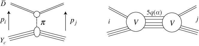
Figure 1: One pion exchange potential (left) and the effective interaction due to the coupling to the 5$q$ channel (right). The meson-baryon channels are generally represented by $\bar{D}$ and $Y_{c}$, respectively, and $i$ is for the initial and $j$ the final channels. A $5q$ channel is denoted by $\alpha$.

II.2 One pion exchange potential

In this subsection, we derive the one pion exchange potential (OPEP) between $\bar{D}^{(\ast)}$ and $Y_{\rm c}$ in the first term of Eq. (17). Hereafter, we use the notation $\bar{D}^{(\ast)}$ to stand for a $\bar{D}$ meson, or a $\bar{D}^{\ast}$ meson, and $Y_{c}$ to stand for $\Lambda_{\rm c}$, $\Sigma_{\rm c}$, or $\Sigma^{\ast}_{\rm c}$.

The OPEP is obtained by the effective Lagrangians for heavy mesons (baryons) and the Nambu-Goldstone boson, satisfying the heavy quark and chiral symmetries. The Lagrangians for heavy mesons and the Nambu-Goldstone bosons are given by Wise:1992hn ; Burdman:1992gh ; Yan:1992gz ; Falk:1992cx ; Casalbuoni:1996pg ; Manohar:2000dt

$${\cal L}_{\pi HH}=g_{\pi}{\rm Tr}\left[H_{b}\gamma_{\mu}\gamma_{5}A^{\mu}_{ba}\bar{H}_{a}\right].$$ (18)

The trace ${\rm Tr}\left[\cdots\right]$ is taken over the gamma matrix. The heavy meson fields $H$ and $\bar{H}$ are represented by

$$H_{a}=\frac{1+{v/}}{2}\left[\bar{D}^{\ast}_{a\mu}\gamma^{\mu}-\bar{D}_{a}\gamma_{5}\right],$$ (19)

$$\bar{H}_{a}=\gamma_{0}H^{\dagger}_{a}\gamma_{0},$$ (20)

where the fields are constructed by the heavy pseudoscalar meson $\bar{D}$ and the vector meson $\bar{D}^{\ast}$ belonging to the heavy quark spin (HQS) doublet. $v_{\mu}$ is a four-velocity of a heavy quark, and satisfies $v^{\mu}v_{\mu}=1$ and $v^{0}>0$. The subscripts $a,b$ are for the light flavor $u,d$. The axial vector current for the pion, $A_{\mu}$, is given by

$$A_{\mu}=\frac{i}{2}\left[\xi^{\dagger}(\partial_{\mu}\xi)+(\partial_{\mu}\xi)\xi^{\dagger}\right],$$ (21)

where $\xi=\exp\left(\frac{i\hat{\pi}}{2f_{\pi}}\right)$ with the pion decay constant $f_{\pi}=92.3$ MeV. The pion field $\hat{\pi}$ is given by

$$\hat{\pi}=\sqrt{2}\left(\begin{array}[]{cc}\frac{\pi^{0}}{\sqrt{2}}&\pi^{+}\\ \pi^{-}&-\frac{\pi^{0}}{\sqrt{2}}\\ \end{array}\right).$$ (24)

The coupling constant $g_{\pi}$ is determined by the strong decay of $D^{\ast}\rightarrow D\pi$ as $g_{\pi}=0.59$ Casalbuoni:1996pg ; Manohar:2000dt ; Olive:2016xmw .

The Lagrangians for heavy baryons and Nambu-Goldstone bosons are given by Yan:1992gz ; Liu:2011xc

$${\cal L}_{\pi BB} =\frac{3}{2}g_{1}(iv_{\kappa})\varepsilon^{\mu\nu\lambda\kappa}{\rm tr}\left[\bar{S_{\mu}}A_{\nu}S_{\lambda}\right]+g_{4}{\rm tr}\left[\bar{S}^{\mu}A_{\mu}B_{\bar{3}}\right]+{\rm H.c.}$$ (25)

The trace ${\rm tr}\left[\cdots\right]$ is for the flavor space. The superfields $S_{\mu}$ and $\bar{S}_{\mu}$ are represented by

$$S_{\mu}=\hat{\Sigma}^{\ast}_{{\rm c}\mu}+\frac{\delta}{\sqrt{3}}\left(\gamma_{\mu}+v_{\mu}\right)\gamma_{5}\hat{\Sigma}_{\rm c},$$ (26)

$$\bar{S}_{\mu}=\gamma_{0}S^{\dagger}_{\mu}\gamma_{0},$$ (27)

with the $\hat{\Sigma}_{\rm c}$ and $\hat{\Sigma}^{\ast}_{\rm c}$ fields in the HQS multiplet. The phase factor $\delta$ is set at $\delta=-1$, as discussed in Ref. Liu:2011xc . The heavy baryon fields $\hat{\Lambda}_{\rm c}$ and $\hat{\Sigma}^{(\ast)}_{\rm c(\mu)}$ are expressed by

$$\hat{\Lambda}_{\rm c}=\left(\begin{array}[]{cc}0&\Lambda^{+}_{\rm c}\\ -\Lambda^{+}_{\rm c}&0\\ \end{array}\right),\quad\hat{\Sigma}^{(\ast)}_{\rm c(\mu)}=\left(\begin{array}[]{cc}\Sigma^{(\ast)++}_{\rm c(\mu)}&\frac{1}{\sqrt{2}}\Sigma^{(\ast)+}_{\rm c(\mu)}\\ \frac{1}{\sqrt{2}}\Sigma^{(\ast)+}_{\rm c(\mu)}&\Sigma^{(\ast)0}_{\rm c(\mu)}\\ \end{array}\right).$$ (32)

The coupling constants $g_{1}$ and $g_{4}$, given as $g_{1}=(\sqrt{8}/3)g_{4}=1$, are used, which are obtained by the quark model estimation discussed in Ref. Liu:2011xc . For the coupling $g_{4}$, this value can also be fixed by the $\Sigma^{(\ast)}_{\rm c}\to\Lambda_{\rm c}\pi$ decay, and agrees with the one obtained by the quark model Liu:2011xc .

For the hidden-bottom sector, these effective Lagrangians are also applied by replacing the charmed hadron fields by the bottom hadron fields, while the same coupling constants are used.

In order to parametrize the internal structure of hadrons, we introduce the dipole form factor at each vertex:

$$F(\Lambda,\vec{q}\,)=\frac{\Lambda^{2}-m^{2}_{\pi}}{\Lambda^{2}+\vec{q}\,^{2}},$$ (33)

with the pion mass $m_{\pi}$ and the three-momentum $\vec{q}$ of an incoming pion. As discussed in Refs. Yasui:2009bz ; Yamaguchi:2011xb ; Yamaguchi:2011qw , the cutoffs of heavy hadrons are fixed by the ratio between the sizes of the heavy hadron and nucleon, $\Lambda_{N}/\Lambda_{H}=r_{H}/r_{N}$ with the cutoff and size of the heavy hadron being $\Lambda_{H}$ and $r_{H}$, respectively. The nucleon cutoff is determined to reproduce the deuteron-binding energy by the OPEP as $\Lambda_{N}=837$ MeV Yasui:2009bz ; Yamaguchi:2011xb ; Yamaguchi:2011qw . The ratios are computed by the means of constituent quark model with the harmonic oscillator potential Oh:2009zj , where the frequency is evaluated by the hadron charge radii in Refs. Hwang:2001th ; SilvestreBrac:1996bg . For the heavy meson Yasui:2009bz , we obtain $\Lambda_{\bar{D}}=1.35\Lambda_{N}$ and $\Lambda_{B}=1.29\Lambda_{N}$ for the $\bar{D}^{(\ast)}$ meson and the $B$ meson, respectively. For the heavy baryon Oh:2009zj , we obtain $\Lambda_{\Lambda_{\rm c}}\sim\Lambda_{\Sigma_{\rm c}}\sim\Lambda_{N}$ for the charmed baryon, and $\Lambda_{\Lambda_{\rm b}}\sim\Lambda_{\Sigma_{\rm b}}\sim\Lambda_{N}$ for the bottom baryon. We note that values of these cutoffs are smaller than those used in other studies, e.g. $\Lambda=2.35$ GeV and $\Lambda=1.77$ GeV in Ref. Chen:2015loa .

From these Lagrangians (18) and (25), and the form factor (33), we obtain the OPEP as the Born term of the scattering amplitude. The explicit form of the OPEP is summarized in Appendix A. The OPEP is also used for the hidden-bottom sector, $B^{(\ast)}Y_{b}$, by employing the cutoff parameters $\Lambda_{B}$, $\Lambda_{\Lambda_{\rm b}}$, and $\Lambda_{\Sigma_{\rm b}}$, where $B^{(\ast)}$ stands for $B$ or $B^{\ast}$, and $Y_{b}$ stands for $\Lambda_{\rm b}$, $\Sigma_{\rm b}$ or $\Sigma^{\ast}_{\rm b}$. Let us remark about the contact term of the OPEP. In this study, it is neglected as shown in Eq. (71) as is in the conventional nuclear physics. We assume that the OPEP appears only in the long range hadronic region. As discussed above, the cutoff parameters of the OPEP are determined from the ratio of sizes of the relevant hadron and nucleon. The cutoff of the nucleon is determined so as to reproduce the deuteron binding energy without the contact term Yasui:2009bz .

II.3 Couplings to $5q$ states

In this subsection, we derive the effective short-range interaction, the 2nd term of (17). To do so, we need to know the matrix elements $\Braket{i}{V}{\alpha}$ and the eigenenergies, $E^{5q}_{\alpha}$. As discussed in the previous section II.1, the matrix elements are assumed to be proportional to the spectroscopic factor, the overlap $\Braket{i}{\alpha}$,

$$\Braket{i}{V}{\alpha}=f\Braket{i}{\alpha}$$ (34)

where $f$ is the only parameter to determine the overall strength of the matrix elements. As we will discuss later, the approximation (34) turns out to be rather good in comparison with the quark cluster model calculations Takeuchi:2016ejt .

For the computation of the spectroscopic factor, let us construct the $MB$ and 5$q$ wave functions explicitly. We employ the standard non-relativistic quark model with a harmonic oscillator confining potential. The wave functions are written as the products of color, spin, flavor and orbital wave functions. Let us introduce the notation $\Ket{\bar{D}Y_{c}(\vec{p}_{i})}$ for the open-charm meson-baryon channel $i$ of relative momentum $\vec{p}_{i}$. Thus, we can write the wave function for $\Ket{\bar{D}Y_{c}(\vec{p}_{i})}$ as Hosaka:2004bn

$$\Braket{\vec{\rho},\vec{\lambda},\vec{r},\vec{x}}{\bar{D}Y_{c}(\vec{p}_{i})}=\psi^{int}_{\bar{D}}(\vec{r})\psi^{int}_{Y_{c}}(\vec{\rho},\vec{\lambda})e^{i\vec{p}_{i}\cdot\vec{x}}\times\phi_{\bar{D}Y_{c}}(CSF).$$ (35)

In (35), we indicate only the spatial coordinates explicitly, while the other coordinates for the color, spin and flavor are summarized in $\phi_{\bar{D}Y_{c}}(CSF)$. These coordinates are shown in Fig. 2. The spatial wave functions $\psi^{int}_{\bar{D}}(\vec{r}\,)\psi^{int}_{\Lambda_{c}}(\vec{\rho},\vec{\lambda}\,)$ are then written by those of harmonic oscillator.

Figure 2: Jacobi coordinates of “$\bar{D}$ meson” and “$Y_{c}$ baryon” in the $5q$ configuration. $q_{i}$ $(i=1,2,3)$ stands for the light quark, and $c_{4}$ ($\bar{c}_{5}$) stands for the (anti)charm quark. The coordinate $\vec{\rho}$ is the relative coordinate of $q_{1}q_{2}$, $\vec{\lambda}$ the relative coordinate between the center of mass of $q_{1}q_{2}$ and $c_{4}$, $\vec{r}$ the relative coordinate of $q_{3}\bar{c}_{5}$, and $\vec{x}$ the relative coordinate between the centers of mass of $q_{1}q_{2}c_{4}$ and $\bar{c}_{5}q_{3}$. Though we do not use the total center-of-mass coordinate $\vec{X}$ in the present paper explicitly, it is also shown in the figure.

For the five-quark state, we assume that the quarks move independently in a single confined region, and hence the $\vec{x}$ motion is also confined. Therefore, by introducing $\Ket{5q\,(\alpha)}$, we have

$$\Braket{\vec{\rho},\vec{\lambda},\vec{r},\vec{x}}{5q\,(\alpha)}=\psi^{int}_{5q}(\vec{\rho},\vec{\lambda},\vec{r})\left(\frac{2A}{\pi}\right)^{3/4}e^{-A^{2}x^{2}}\times\phi_{5q}(CSF),$$ (36)

where the index $\alpha$ is for the $5q$ configurations, as shown in Table 2 for a given spin. The parameter $A$ represents the inverse of the spatial separation of $\vec{x}$-motion, corresponding to the $qqc$ and $q\bar{c}$ clusters, which is in the order of 1 fm, or less. Again, the color, spin and flavor part is summarized in $\phi_{5q}(CSF)$.

Now the spectroscopic factor is the overlap of (35) and (36). Assuming that the spatial wave functions $\psi^{int}_{\bar{D}}(\vec{r}\,)\psi^{int}_{\Lambda_{c}}(\vec{\rho},\vec{\lambda}\,)$ and $\psi^{int}_{5q}(\vec{\rho},\vec{\lambda},\vec{r})$ are the same, the overlap is given by the color, spin and flavor parts, as labeled by $CSF$ below, and by the Fourie transform of the Gaussian function,

$$\Braket{\bar{D}Y_{c}(\vec{p}_{i})}{5q\,(\alpha)} = \Braket{\phi_{\bar{D}Y_{c}}(CSF)}{\phi_{5q}(CSF)}\int d^{3}x\left(\frac{2A}{\pi}\right)^{3/4}e^{-Ax^{2}}e^{i\vec{p_{i}}\cdot\vec{x}}$$ (37)

$$= \Braket{\phi_{\bar{D}Y_{c}}(CSF)}{\phi_{5q}(CSF)}\left(\frac{2\pi}{A}\right)^{3/4}e^{-p^{2}_{i}/4A}\equiv S^{\alpha}_{i}g(\vec{p}_{i}),$$

where $S^{\alpha}_{i}$ is the spectroscopic factor for the color, flavor and spin parts of the wave function, and $g(\vec{p}_{i})$ the form factor for the transition $\bar{D}Y_{c}(\vec{p}_{i})\to 5q(\alpha)$. The method how to compute $S^{\alpha}_{i}$ is presented in Appendix B, and the results for various meson-baryon channels $i$ and the $5q$ channels are summarized in Table 3.

Table 3: Spectroscopic factor of the $5q$ potential. $J$ is the total angular momentum of the system, $S_{c\bar{c}}$ is the total spin of $c\bar{c}$, and $S_{3q}$ is the total spin of the three light quarks.

$J$	$S_{c\bar{c}}$	$S_{3q}$	$\bar{D}\Lambda_{\rm c}$	$\bar{D}^{\ast}\Lambda_{\rm c}$	$\bar{D}\Sigma_{\rm c}$	$\bar{D}\Sigma^{\ast}_{\rm c}$	$\bar{D}^{\ast}\Sigma_{\rm c}$	$\bar{D}^{\ast}\Sigma^{\ast}_{\rm c}$
$\frac{1}{2}$	$0$	$\frac{1}{2}$	$0.35$	$0.61$	$-0.35$	—	$0.20$	$-0.58$
	$1$	$\frac{1}{2}$	$0.61$	$-0.35$	$0.20$	—	$-0.59$	$-0.33$
	$1$	$\frac{3}{2}$	$0.00$	$0.00$	$-0.82$	—	$-0.47$	$0.33$
$\frac{3}{2}$	$0$	$\frac{3}{2}$	—	$0.00$	—	$-0.50$	$0.58$	$-0.65$
	$1$	$\frac{1}{2}$	—	$0.71$	—	$0.41$	$-0.24$	$-0.53$
	$1$	$\frac{3}{2}$	—	$0.00$	—	$-0.65$	$-0.75$	$-0.17$
$\frac{5}{2}$	$1$	$\frac{3}{2}$	—	—	—	—	—	$-1.00$

The wave functions should reflect the antisymmetric nature (a quark exchange effect) under the permutation among all light quarks especially in different clusters $\bar{D}Y_{c}$. This is neglected in $\Ket{\bar{D}Y_{c}(\vec{p}_{i})}$. The effect, however, is introduced in the present model at least partially by considering the above overlap, because the $\psi^{int}_{5q}\phi_{5q}$ is totally antisymmetric over the quarks. Such quark exchange effect is suppressed, as the two color-singlet clusters $\bar{D}Y_{c}$ are further apart for larger $x$ and therefore the above overlap is suppressed.

Finally, the transition amplitude from $i$ to $j$ of $\bar{D}Y_{c}$ channels is expressed by

$$T_{ij}=f^{\prime}\sum_{\alpha}S^{\alpha}_{i}S^{\alpha}_{j}g(\vec{p}_{i})g(\vec{p}_{j})\frac{1}{E-E^{5q}_{\alpha}}.$$ (38)

The overall strength $f^{\prime}$ of this amplitude is not determined, and is treated as a parameter, while the relative strengths of various channels $i,j$ are determined by the factors $S^{\alpha}_{i}$ and $S^{\alpha}_{j}$.

The transition amplitude $T_{ij}$ in (38) has been given in a separable form. To use it in the Schrödinger equation, it is convenient to express it in the form of local potential, which is a function of the momentum transfer $\vec{q}=\vec{p}_{i}-\vec{p}_{f}$. We attempt to set

$$g(\vec{p}_{i})g(\vec{p}_{j})=e^{-({p}^{2}_{i}+{p}^{2}_{j})/4\alpha}\sim e^{-\beta{q}^{2}}.$$ (39)

On ignoring the angle-dependent term of ${q}^{2}=(\vec{p}_{i}-\vec{p}_{f})^{2}={p}^{2}_{i}+{p}^{2}_{j}-2\vec{p}_{i}\cdot\vec{p}_{j}$, it is reasonable to set $\beta=1/4A$. Therefore, the transition amplitude is parametrized as

$$T_{ij}\sim\sum_{\alpha}S^{\alpha}_{i}S^{\alpha}_{j}e^{-q^{2}/4A}\frac{1}{E-E^{\alpha}_{5q}}.$$ (40)

This gives an energy dependent local potential

$$V^{5q}_{ij}(E;r)\sim\sum_{\alpha}S^{\alpha}_{i}S^{\alpha}_{j}e^{-Ar^{2}}\frac{1}{E-E^{\alpha}_{5q}},$$ (41)

with the relative coordinate $r$ between the heavy meson and baryon.

Now, if we further expect that the compact five-quark configuration $\Ket{5q\,(\alpha)}$ is located sufficiently above the energy region in which we are interested, namely $E^{\alpha}_{5q}\gg m_{\bar{D}}+m_{Y_{c}}$, then we may further approximate

$$V^{5q}_{ij}(r)=-f\sum_{\alpha}S^{\alpha}_{i}S^{\alpha}_{j}e^{-Ar^{2}},$$ (42)

where $f$ is a positive overall coupling strength. As shown in Table 4, in a simple quark model estimation, the $qqqc{\bar{c}}$ five-quark masses with the color-octet three light quarks are about 400 MeV larger than the threshold energies of $\bar{D}Y_{c}$ in the present study. The masses of hidden-bottom five-quarks are similarly higher than the $\bar{B}Y_{b}$ thresholds. This makes the potential (42) attractive for both of the hidden-charm and hidden-bottom sectors. As we will discuss later in this paper, especially this attraction turns out to be the driving force for abundant $P_{c}$ states.

Table 4: Masses of the hidden-charm five-quark states with the color-octet three light quarks, $E^{\alpha}_{5q}$, calculated by using parameters in Ref. Takeuchi:2016ejt . All the entries are listed in MeV. $J$ stands for the total spin of the five-quarks, [$q^{3}8s]S$ stands for the five-quark state, which consists of the $uud$ quarks with a spin of $s$ and the $c\overline{c}$ pair with a spin of $S$.

$J$	$[q^{3}8\frac{1}{2}]0$	$[q^{3}8\frac{1}{2}]1$	$[q^{3}8\frac{3}{2}]0$	$[q^{3}8\frac{3}{2}]1$
$\frac{1}{2}$	4816.2	4759.1	-	4772.2
$\frac{3}{2}$	-	4822.3	4892.5	4835.4
$\frac{5}{2}$	-	-	-	4940.7

III Numerical results

III.1 Model parameters

To start with, let us fix the two parameters, $f$ and $A$, in the $5q$ potential (42). The Gaussian range $A=\mu\omega/2$ originates the frequency of the harmonic oscillator potential $V(x)=\frac{1}{2}\mu\omega^{2}x^{2}$ of a “meson” and a “baryon” in the $5q$ state, as shown in Fig. 2. Hence, $A$ is expressed by the relative distance $\Braket{x^{2}}\equiv\Braket{\psi}{x^{2}}{\psi}$ of the “meson” and “baryon” as

$$A=\frac{3}{4\Braket{x^{2}}},$$ (43)

with the harmonic oscillator wave function

$$\psi(x)=\left(\frac{2A}{\pi}\right)^{3/4}e^{-Ax^{2}}\,.$$ (44)

In this study, we assume that $\sqrt{\Braket{x^{2}}}$ is less than 1 fm, namely $A\geq\frac{3}{4}$ fm^-2, and employ $A=1$ fm^-2.

The overall strength $f$ is a free parameter, and we will show our numerical results for various $f$. It is then convenient to set a reference value $f_{0}$. Here we use the $\bar{D}^{\ast}\Sigma_{\rm c}$ diagonal term of the OPEP,

$$f_{0}=\left|C^{\pi}_{\bar{D}^{\ast}\Sigma_{\rm c}}(r=0)\right|\sim 6\text{ MeV},$$ (45)

where $C^{\pi}_{\bar{D}^{\ast}\Sigma_{\rm c}}(r)\equiv-\frac{gg_{1}}{3f_{\pi}^{2}}C(r)$ is the central force of $V^{\pi}_{\bar{D}^{\ast}\Sigma_{\rm c}-\bar{D}^{\ast}\Sigma_{\rm c}}(r)$ without the spin-dependent operator $\vec{S}\cdot\vec{\sigma}$, as shown in Eq. (65).

When $f_{0}=6$ MeV and $A=1$ fm^-2 are used, the short range interaction is not as strong as what we expect from the $NN$ force. To see this point, we compare the volume integrals of the potentials 

$$\left|\int d^{3}rf_{0}e^{-Ar^{2}}\right|=4.3\times 10^{-6}\text{ MeV}^{-2},$$ (46)

$$\left|\int d^{3}rC^{\pi}_{\bar{D}^{\ast}\Sigma_{\rm c}}(r)\right|=1.8\times 10^{-5}\text{ MeV}^{-2},$$ (47)

$$\left|\int d^{3}rV^{\pi}_{NN}(r)\right|=6.3\times 10^{-5}\text{ MeV}^{-2},$$ (48)

$$\left|\int d^{3}rV^{\sigma}_{NN}(r)\right|=3.8\times 10^{-3}\text{ MeV}^{-2},$$ (49)

with the central force of the OPEP and the $\sigma$ exchange, $V^{\pi}_{NN}$ and $V^{\sigma}_{NN}$, in the Bonn potential Machleidt:1987hj . From Eqs. (46)-(49), we obtain

$$\left|\int d^{3}rf_{0}e^{-Ar^{2}}(r)\right|\sim\frac{1}{4}\left|\int d^{3}rC^{\pi}_{\bar{D}^{\ast}\Sigma_{\rm c}}(r)\right|\sim\frac{1}{15}\left|\int d^{3}rV^{\pi}_{NN}(r)\right|\sim\frac{1}{880}\left|\int d^{3}rV^{\sigma}_{NN}(r)\right|.$$ (50)

We find that the volume integral of the $5q$ potential with $f=f_{0}$ (46) is smaller than that of the $NN$ potentials (48) and (49). In particular, the volume integral in Eq. (46) is much smaller than in Eq. (49) for the $\sigma$ exchange potential in the $NN$ interaction. In Section III, we will see that the non-trivial bound and resonant states are produced, when $f\sim 25f_{0}$ (or larger), whose volume integral is still much smaller than that in Eq. (49). In Fig. 3, we show the $5q$ potential with the fixed parameters $f_{0}$ and $A$, where the obtained $5q$ potential is compared with $C^{\pi}_{\bar{D}^{\ast}\Sigma_{\rm c}}(r)$.

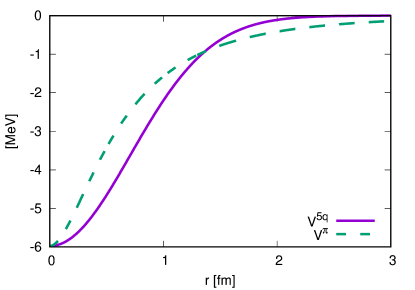
Figure 3: (Color online) The plot of the $5q$ potential, $V^{5q}$, (solid line) and the central force of the OPEP in the diagonal $\bar{D}^{\ast}\Sigma_{\rm c}-\bar{D}^{\ast}\Sigma_{\rm c}$ term, $V^{\pi}$, (dashed line).

III.2 Numerical methods

The bound and resonant states are obtained by solving the coupled-channel Schrödinger equation with the OPEP, $V^{\pi}(r)$, and $5q$ potential, $V^{5q}(r)$,

$$\left(K+V^{\pi}(r)+V^{5q}(r)\right)\Psi(r)=E\Psi(r),$$ (51)

with the kinetic term $K$. The OPEP and kinetic terms are summarized in Appendix A.

The Schrödinger equation (51) is solved by using the variational method. The trial function $\Psi_{JM,IM_{I}}(\vec{r}\,)$ with the total angular momentum $J$, total isospin $I$, and their $z$-components $M$ and $M_{I}$ is expressed by the Gaussian expansion method Hiyama:2003cu as

$$\Psi_{JM,IM_{I}}(\vec{r}\,) =\sum_{i=1}^{i_{max}}\sum_{L,S}C_{iLS}\left[\psi_{iLM_{L}}(\vec{r}\,)\otimes\left[\chi_{s_{1}m_{s_{1}}}\chi_{s_{2}m_{s_{2}}}\right]_{SM_{S}}\right]_{JM}\left[\eta_{I_{1}m_{I_{1}}}\eta_{I_{2}m_{I_{2}}}\right]_{IM_{I}},$$ (52)

$$\psi_{iLM_{L}}(\vec{r}\,) =\sqrt{\frac{2}{\Gamma(L+3/2)b^{3}_{i}}}\left(\frac{r}{b_{i}}\right)^{L}\exp\left(-\frac{r^{2}}{2b^{2}_{i}}\right)Y_{LM_{L}}(\hat{r}).$$ (53)

In the Gaussian expansion method, the wave function is expanded in terms of Gaussian basis functions, as shown in Eq. (53). The coefficients $C_{iLS}$ are determined by diagonalizing the Hamiltonian, and $\psi_{iLM_{L}}(\vec{r}\,)$ are the radial wave function of the meson-baryon with the orbital angular momentum $L$ and the $z$-component $M_{L}$. The (iso)spin wave functions $\chi_{s_{k}m_{s_{k}}}$ ($\eta_{I_{k}m_{I_{k}}}$) with $k=1,2$ are for the (iso)spin $s_{k}$ ($I_{k}$) of the hadron $k$, with the $z$-component $m_{s_{k}}$ ($m_{I_{k}}$). The total (iso)spin is given by $S$ ($I$) with the $z$-component $M_{S}$ ($M_{I}$). The angular part of the radial wave function is represented by the spherical harmonics $Y_{LM_{L}}(\hat{r})$. The Gaussian ranges $b_{i}$ are given by the form of geometric series as

$$b_{i}=b_{1}a^{i-1}\quad(i=1,\cdots,i_{max}),$$ (54)

with the variational parameters $b_{1}$ and $b_{i_{max}}$, and $a=(b_{i_{max}}/b_{1})^{1/({i_{max}-1})}$.

In order to find not only bound states, but also resonances, the complex scaling method Aguilar1971_269 ; Blaslev1971_22 ; Simon1972_27 ; Prog.Theor.Phys11620061Aoyama is employed. By diagonalizing the complex scaled Hamiltonian with $r\rightarrow re^{i\theta}$ and $p\rightarrow pe^{-i\theta}$, binding energies and resonance energies with decay widths are obtained as the eigenenergy of the complex scaled Schrödinger equation.

III.3 Numerical results of the hidden-charm sector

$J^{P}=1/2^{-}$
(i) $(S_{c\bar{c}},S_{3q})=(0,\frac{1}{2})$	(ii) $(S_{c\bar{c}},S_{3q})=(1,\frac{1}{2})$	(iii) $(S_{c\bar{c}},S_{3q})=(1,\frac{3}{2})$

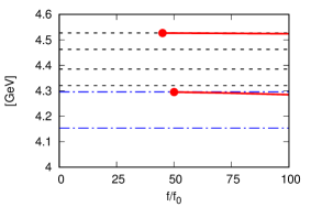
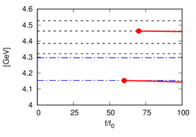
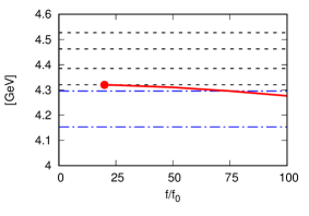
Figure 4: (Color online) Bound and resonant state energies of the hidden-charm molecules (solid lines) with various coupling constants $f$ for $J^{P}=1/2^{-}$, using the OPEP and one of the three $5q$ potentials derived from the configuration (i) $(S_{c\bar{c}},S_{3q})=(0,1/2)$, (ii) $(1,1/2)$, or (iii) $(1,3/2)$. The horizontal axis shows the ratio $f/f_{0}$, where $f_{0}$ is the reference value defined in Sec. III.1. Filled circle is the starting point where the states appear. Dashed lines are the $\bar{D}\Sigma_{\rm c}$, $\bar{D}\Sigma^{\ast}_{\rm c}$, $\bar{D}^{\ast}\Sigma_{\rm c}$, and $\bar{D}^{\ast}\Sigma^{\ast}_{\rm c}$ thresholds. Dot-dashed lines are the $\bar{D}\Lambda_{\rm c}$ and $\bar{D}^{\ast}\Lambda_{\rm c}$ thresholds.

$J^{P}=1/2^{-}$

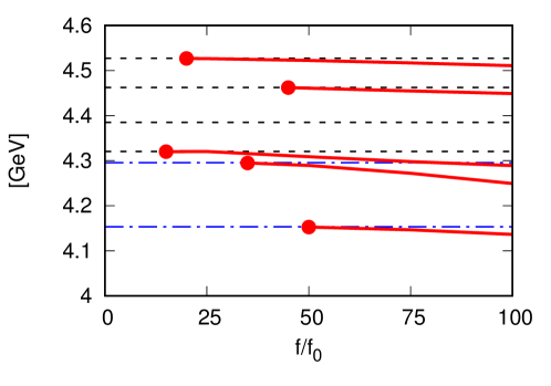
Figure 5: (Color online) The same as Fig. 4 for the bound and resonant states of the hidden-charm molecules for $J^{P}=1/2^{-}$ using the OPEP and the sum of the three $5q$ potentials.

Let us show the numerical results of the hidden-charm meson-baryon molecules. The coupling strength $f$ dependence of the energy spectrum is summarized in Figs. 4-5 and Tables 5-6 for $J^{P}=1/2^{-}$, in Figs. 6-7 and Tables 7-8 for $J^{P}=3/2^{-}$, and in Fig. 8 and Table 9 for $J^{P}=5/2^{-}$.

Figure 4 shows the strength $f$ dependence of the obtained energy spectra for $J^{P}=1/2^{-}$ by employing the OPEP and one of the three $5q$ potentials derived from the configurations (i) $(S_{c\bar{c}},S_{3q})=(0,1/2)$, (ii) $(1,1/2)$, or (iii) $(1,3/2)$. We obtain no state only with the OPEP, corresponding to the result at $f/f_{0}=0$, while the bound and resonant states appear by increasing the strength $f$ of the $5q$ potential. The filled circle in figures shows the starting point where the state is found. In Fig. 4 (i), two resonances appear below $\bar{D}^{\ast}\Lambda_{\rm c}$ and $\bar{D}^{\ast}\Sigma^{\ast}_{\rm c}$ thresholds for $f$ larger than $f/f_{0}=50$ and $45$, respectively. In Fig. 4 (ii), the bound state and resonance are obtained below $\bar{D}\Lambda_{\rm c}$ and $\bar{D}^{\ast}\Sigma_{\rm c}$ thresholds for $f$ larger than $f/f_{0}=60$ and $70$, respectively. In Fig. 4 (iii), the resonance below the $\bar{D}\Sigma_{\rm c}$ threshold appears at and above $f/f_{0}=20$ which is smaller than the strength in other channels. Thus, the $5q$ potential from the configuration with $S_{3q}={3}/{2}$ produces the strong attraction rather than the potential from the configuration with $S_{3q}={1}/{2}$, corresponding to the results in Figs. 4 (i) and (ii).

As shown in Fig. 4, the energy spectra appear just below the meson-baryon thresholds. The obtained spectrum structure can be explained by the spectroscopic factor ($S$-factor) of the $5q$ potential in Table 3. Since the $S$-factor gives the relative strength of the $5q$ potential among $\bar{D}^{(\ast)}\Lambda_{\rm c}$ and $\bar{D}^{(\ast)}\Sigma^{(\ast)}_{\rm c}$ channels, the channels with a large $S$-factor play an important role to produce bound and resonant states. For (i) $(S_{c\bar{c}},S_{3q})=(0,1/2)$, the large $S$-factors are obtained for the $\bar{D}^{\ast}\Lambda_{\rm c}$ and $\bar{D}^{\ast}\Sigma^{\ast}_{\rm c}$ channels and indeed, the resonances are obtained below the $\bar{D}^{\ast}\Lambda_{\rm c}$ and $\bar{D}^{\ast}\Sigma^{\ast}_{\rm c}$ thresholds. In (ii) $(S_{c\bar{c}},S_{3q})=(1,1/2)$, the bound and resonant states below $\bar{D}\Lambda_{\rm c}$ and $\bar{D}^{\ast}\Sigma_{\rm c}$ are obtained, where the large $S$-factors are obtained in the $\bar{D}\Lambda_{\rm c}$ and $\bar{D}^{\ast}\Sigma_{\rm c}$ channels. In (iii) $(S_{c\bar{c}},S_{3q})=(1,3/2)$, one resonance below the $\bar{D}\Sigma_{\rm c}$ threshold is found, where the large $S$-factor is obtained in the $\bar{D}\Sigma_{\rm c}$ channel.

In Fig. 5, we show the energy spectra with the full potential including OPEP and the sum of the three $5q$ potentials with the same weight. As expected, the result is a combination of the three results in Fig. 4 with some more attraction. As $f/f_{0}$ is increased, the resonance appear even for $f/f_{0}=15$, which would corresponds to the state found in Fig. 4 (iii). We see that the $5q$ potential produces many states when the strength $f/f_{0}$ is increased.

$J^{P}=3/2^{-}$
(i) $(S_{c\bar{c}},S_{3q})=(0,\frac{3}{2})$	(ii) $(S_{c\bar{c}},S_{3q})=(1,\frac{1}{2})$	(iii) $(S_{c\bar{c}},S_{3q})=(1,\frac{3}{2})$

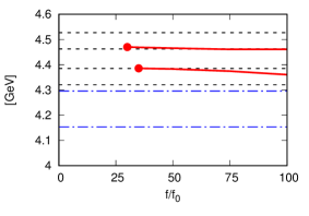
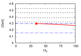
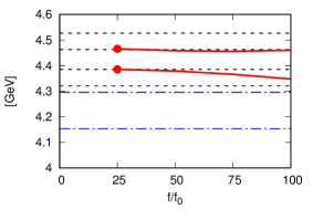
Figure 6: (Color online) The same as Fig. 4 for the resonant states of the hidden-charm molecules for $J^{P}=3/2^{-}$ using the OPEP and one of the three $5q$ potentials derived from the configuration (i) $(S_{c\bar{c}},S_{3q})=(0,3/2)$, (ii) $(1,1/2)$, or (iii) $(1,3/2)$.

$J^{P}=3/2^{-}$

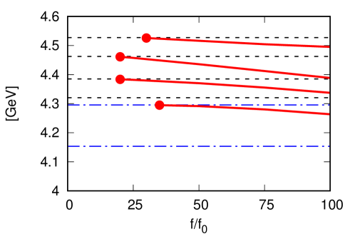
Figure 7: (Color online) The same as Fig. 4 for the resonant states of the hidden-charm molecules for $J^{P}=3/2^{-}$ using the OPEP and the sum of the three $5q$ potentials.

The states are also obtained in $J^{P}=3/2^{-}$ and $5/2^{-}$ as well as $1/2^{-}$, where the structure of the energy spectra is explained by the $S$-factor. In Figs. 6 and 7, the strength $f$ dependence of the energies for $J^{P}=3/2^{-}$ is shown. We also obtain no state only with the OPEP, corresponding to the results at $f/f_{0}=0$, but the states appear when the strength of the $5q$ potential is increased as seen in $J^{P}=1/2^{-}$. There are three $5q$ potentials derived from the quark configurations (i) $(S_{c\bar{c}},S_{3q})=(0,3/2)$, (ii) $(1,1/2)$, and (iii) $(1,3/2)$. In Fig. 6 (i), two resonances are obtained near the $\bar{D}\Sigma^{\ast}_{\rm c}$ and $\bar{D}^{\ast}\Sigma_{\rm c}$ thresholds, where the large $S$-factors are obtained in the $\bar{D}\Sigma^{\ast}_{\rm c}$, $\bar{D}^{\ast}\Sigma_{\rm c}$, and $\bar{D}^{\ast}\Sigma^{\ast}_{\rm c}$ components. In Fig. 6 (ii), one resonance is found near the $\bar{D}^{\ast}\Lambda_{\rm c}$ threshold for $f/f_{0}\geq 35$, where the $S$-factor of the $\bar{D}^{\ast}\Lambda_{\rm c}$ is also large. In Fig. 6 (iii), the two resonances are found near the $\bar{D}\Sigma^{\ast}_{\rm c}$ and $\bar{D}^{\ast}\Sigma_{\rm c}$ thresholds, and the large $S$-factors are also obtained in the $\bar{D}\Sigma^{\ast}_{\rm c}$ and $\bar{D}^{\ast}\Sigma_{\rm c}$ channels. In Fig. 7, the results with the summation of the three $5q$ potentials are shown. The four resonances appear below the $\bar{D}\Lambda^{\ast}_{\rm c}$ threshold for $f/f_{0}\geq 35$, below the $\bar{D}\Sigma^{\ast}_{\rm c}$ threshold for $f/f_{0}\geq 20$, below the $\bar{D}^{\ast}\Sigma_{\rm c}$ threshold for $f/f_{0}\geq 20$, and below the $\bar{D}^{\ast}\Sigma^{\ast}_{\rm c}$ threshold for $f/f_{0}\geq 30$, respectively.

The obtained energy spectra for $J^{P}=5/2-$ are shown in Fig. 8. There is only one $5q$ potential from the quark configuration $(S_{c\bar{c}},S_{3q})=(1,3/2)$, which appears only in the $\bar{D}^{\ast}\Sigma^{\ast}_{\rm c}$ channel. No state is found only by employing the OPEP, while one resonance below the $\bar{D}^{\ast}\Sigma^{\ast}_{\rm c}$ threshold is obtained for $f/f_{0}\geq 25$.

The obtained results in the hidden-charm sector should be compared to the $P^{+}_{\rm c}$ pentaquarks. The LHCb collaboration reported that the two $P^{+}_{\rm c}$ pentaquarks were found close to the $\bar{D}\Sigma^{\ast}_{\rm c}$ and $\bar{D}^{\ast}\Sigma_{\rm c}$ thresholds, and the preferred spins are $J=3/2$ and $5/2$. In the numerical results, we also obtain the resonances close to the $\bar{D}\Sigma^{\ast}_{\rm c}$ and $\bar{D}^{\ast}\Sigma_{\rm c}$ thresholds for $J^{P}=3/2^{-}$, as shown in Figs. 6-7, and Tables 7-8. The obtained resonances close to the $\bar{D}^{\ast}\Sigma_{\rm c}$ have the mass around 4460 MeV and the width around 20 MeV, and these values are in good agreement with the observed $P^{+}_{\rm c}$, while the spin-parity of the obtained state $J^{P}=3/2^{-}$ is not the suggested one by the LHCb collaboration. For the resonance close to the $\bar{D}\Sigma^{\ast}_{\rm c}$ threshold, the obtained mass around 4380 MeV agrees with the reported $P^{+}_{\rm c}$ mass. However, the obtained width around 6 MeV is very different from the reported width 205 MeV. In comparison to the observed $P^{+}_{\rm c}$ states, the $J^{P}=3/2^{-}$ state could be a candidate of the upper $P^{+}_{\rm c}$ state.

$J^{P}=5/2^{-}$

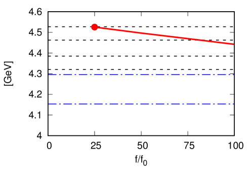
Figure 8: (Color online) The same as Fig. 4 for the resonant states of the hidden-charm molecules for $J^{P}=5/2^{-}$ using the OPEP and the $5q$ potential from the configuration $(S_{c\bar{c}},S_{3q})=(1,\frac{3}{2})$.

Table 5: Energy spectra of the hidden-charm molecules for $J^{P}=1/2^{-}$ using the OPEP and one of the $5q$ potentials from the configuration (i) $(S_{c\bar{c}},S_{3q})=(0,1/2)$, (ii) $(1,1/2)$, or (iii) $(1,3/2)$. The energy $E$ and half decay width $\Gamma/2$ in the various coupling constants $f/f_{0}$ are shown. The third row is for the point, where the state appears. The fourth, fifth, sixth and seventh rows show the obtained values with $f=25f_{0}$, $50f_{0}$, $75f_{0}$, and $100f_{0}$, respectively. The values are given in units of MeV. The lowest threshold $\bar{D}\Lambda_{\rm c}$ is at 4153.46 MeV, and the state whose energy is lower than the threshold is a bound state.

(i) $(0,1/2)$	$f/f_{0}$	45	25	50	75	100
	$E$ [MeV]	4527	—	4527	4526	4524
	$\Gamma/2$ [MeV]	0.87	—	0.98	1.77	2.53
	$f/f_{0}$	50	25	50	75	100
	$E$ [MeV]	4295	—	4295	4291	4285
	$\Gamma/2$ [MeV]	0.22	—	0.22	1.42	4.33
(ii) $(1,1/2)$	$f/f_{0}$	70	25	50	75	100
	$E$ [MeV]	4463	—	—	4462	4459
	$\Gamma/2$ [MeV]	1.44	—	—	1.66	2.37
	$f/f_{0}$	60	—	—	75	100
	$E$ [MeV]	4153	—	—	4151	4144
	$\Gamma/2$ [MeV]	—	—	—	—	—
(iii) $(1,3/2)$	$f/f_{0}$	20	25	50	75	100
	$E$ [MeV]	4320	4319	4310	4295	4276
	$\Gamma/2$ [MeV]	0.33	0.35	0.15	$3.90\times 10^{-3}$	$8.21\times 10^{-2}$

Table 6: The same as Table 5 for the energy spectra of the hidden-charm molecules for $J^{P}=1/2^{-}$ using the OPEP and the sum of the three $5q$ potentials.

SUM	$f/f_{0}$	20	25	50	75	100
	$E$ [MeV]	4527	4526	4523	4517	4511
	$\Gamma/2$ [MeV]	0.63	0.85	2.00	2.79	3.33
	$f/f_{0}$	45	25	50	75	100
	$E$ [MeV]	4462	—	4461	4455	4449
	$\Gamma/2$ [MeV]	3.27	—	3.93	6.54	8.66
	$f/f_{0}$	15	25	50	75	100
	$E$ [MeV]	4320	4320	4309	4298	4289
	$\Gamma/2$ [MeV]	0.45	1.70	3.40	2.34	2.57$\times 10^{-2}$
	$f/f_{0}$	35	25	50	75	100
	$E$ [MeV]	4295	—	4290	4272	4249
	$\Gamma/2$ [MeV]	2.01$\times 10^{-2}$	—	6.17$\times 10^{-2}$	9.23$\times 10^{-2}$	7.93$\times 10^{-2}$
	$f/f_{0}$	50	25	50	75	100
	$E$ [MeV]	4153	—	4153	4147	4136
	$\Gamma/2$ [MeV]	—	—	—	—	—

Table 7: The same as Table 5 for the energy spectra of the hidden-charm molecules for $J^{P}=3/2^{-}$ using the OPEP and one of the three $5q$ potentials from the configuration (i) $(S_{c\bar{c}},S_{3q})=(0,3/2)$, (ii) $(1,1/2)$, or (iii) $(1,3/2)$.

(i) $(0,3/2)$	$f/f_{0}$	30	25	50	75	100
	$E$ [MeV]	4470	—	4466	4461	4461
	$\Gamma/2$ [MeV]	10.49	—	17.16	26.61	38.75
	$f/f_{0}$	35	25	50	75	100
	$E$ [MeV]	4386	—	4383	4374	4360
	$\Gamma/2$ [MeV]	2.21	—	3.33	4.08	3.66
(ii) $(1,1/2)$	$f/f_{0}$	35	25	50	75	100
	$E$ [MeV]	4295	—	4292	4281	4265
	$\Gamma/2$ [MeV]	2.64$\times 10^{-2}$	—	4.47$\times 10^{-2}$	8.92$\times 10^{-4}$	0.109
(iii) $(1,3/2)$	$f/f_{0}$	25	25	50	75	100
	$E$ [MeV]	4466	4466	4459	4456	4460
	$\Gamma/2$ [MeV]	9.96	9.96	16.51	23.50	28.94
	$f/f_{0}$	25	25	50	75	100
	$E$ [MeV]	4385	4385	4379	4366	4348
	$\Gamma/2$ [MeV]	1.85	1.85	2.96	2.45	1.57

Table 8: The same as Table 5 for the energy spectra of the hidden-charm molecules for $J^{P}=3/2^{-}$ using the OPEP and the sum of the three $5q$ potentials.

SUM	$f/f_{0}$	30	25	50	75	100
	$E$ [MeV]	4526	—	4516	4505	4495
	$\Gamma/2$ [MeV]	9.58	—	13.52	17.60	22.34
	$f/f_{0}$	20	25	50	75	100
	$E$ [MeV]	4461	4457	4436	4412	4389
	$\Gamma/2$ [MeV]	11.61	12.83	14.70	13.17	10.56
	$f/f_{0}$	20	25	50	75	100
	$E$ [MeV]	4384	4382	4370	4355	4338
	$\Gamma/2$ [MeV]	3.11	3.62	4.69	4.86	4.59
	$f/f_{0}$	35	25	50	75	100
	$E$ [MeV]	4295	—	4291	4280	4264
	$\Gamma/2$ [MeV]	1.41$\times 10^{-2}$	—	5.09$\times 10^{-2}$	7.71$\times 10^{-2}$	8.15$\times 10^{-2}$

Table 9: The same as Table 5 for the energy spectra of the hidden-charm molecules for $J^{P}=5/2^{-}$ using the OPEP and the $5q$ potential from the configuration $(S_{c\bar{c}},S_{3q})=(1,3/2)$.

$(1,3/2)$	$f/f_{0}$	25	25	50	75	100
	$E$ [MeV]	4526	4526	4496	4470	4442
	$\Gamma/2$ [MeV]	28.04	28.04	27.15	22.61	17.54

III.4 Comparison with the Quark Cluster Model

It is interesting to compare our results with those of the quark model Takeuchi:2016ejt . Because of the color confinement, the quark degrees of freedom affect only when the relevant hadrons come close to each other. Investigating $q^{4}\overline{q}~{}(0s)^{5}$ states will give a clue to the short-range part of the hadron interaction arising quark degrees of freedom.

The number of allowed states $q^{4}\overline{q}$ $(0s)^{5}$ is smaller than that of the meson-baryon states. As shown in Table 2, the configuration of the isospin-1/2 three light quarks is either color-singlet spin-1/2, color-octet spin-1/2, or color-octet spin-3/2. Together with the spin-0 or -1 $c\overline{c}$ pair, there exist five spin-1/2, four spin-3/2, and one spin-5/2 $q^{4}\overline{q}$ $(0s)^{5}$ states. The number of $S$-wave meson-baryon states is seven for $J=1/2$, five for $J=3/2$, and one for $J=5/2$. So, there are two [one] forbidden states for the $J=1/2$ [$3/2$] system, where a certain combination of the meson-baryon states is forbidden to exist as a $(0s)^{5}$ configuration. The normalization of such states reduces to zero. This leads to a strong repulsion to that particular combination of the meson-baryon states. On the other hand, there are channels where the normalization is larger than 1, which brings the system an attraction. The five quark states listed in Table 4 have a normalization of 4/3.

Moreover, the color magnetic interaction (CMI) between quarks can contribute to the hadron interaction. In Ref. Takeuchi:2016ejt , the CMI, especially, in the color-octet spin-3/2 configuration of three light quarks brings to an attraction between $\bar{D}Y_{c}$.

It was reported in Ref. Takeuchi:2016ejt that the quark cluster model gives a very shallow bound state for $J=5/2$ (4519.9 MeV), a cusp and a resonance for $3/2$ (4379.3, 4457.8 MeV), and a resonance for $J=1/2$ channels (4317.0 MeV). Energy of each of the structures is close to the meson-baryon threshold, and the widths of the resonances are as narrow as a few MeV.

In the present work, a bound state appears in the $J^{P}=5/2^{-}$ channel when the strength of the short-range interaction is about $f/f_{0}=25$ (Fig. 8). We may consider that this strength roughly corresponds to that of the quark cluster model because there is a shallow bound state in the channel. Suppose the strength determined in the $J^{P}=5/2^{-}$ channel can also apply to the other channels, then there are two resonances in the $J^{P}=3/2^{-}$ channels at around the same energies as those of the quark cluster model (Fig. 7). In the $J^{P}=1/2^{-}$ channel, there are two resonances at $f/f_{0}=25$; one of them corresponds to the quark model results, but additional resonance appears at around $\bar{D}^{\ast}\Sigma^{\ast}_{\rm c}$ threshold (Fig. 5). With this exception, the results of the present work are similar to the quark model one. In the present approach, coupling to the five-quark states gives an attraction to the meson-baryon channel, which plays the same role as the ones from the above mentioned attraction in the quark model.

III.5 Numerical results of the hidden-bottom sector

We discuss the hidden-bottom meson-baryon molecules in this section. The basic features of the potentials are unchanged from those of the hidden-charm, except that the cutoff parameters of the OPEP are different as summarized in Sec. II.2. However, the hadron masses in the bottom sector are larger than those in the charm sector, and the mass splittings of the HQS multiplet ($B$ and $B^{\ast}$, and $\Sigma_{\rm b}$ and $\Sigma^{\ast}_{\rm b}$) are small. Because of these facts, more states are expected for the bottom sector. As a matter of fact, we find that only the OPEP provides sufficiently strong attraction to generate several bound and resonant states. The obtained energies only with the OPEP are summarized in Table. 10. Since the OPEP yields the strong attraction, we will see that both the OPEP and the $5q$ potentials have an important role to produce the energy spectra, while the $S$-factor of the $5q$ potential designs the spectra in the hidden-charm sector.

Table 10: Energy spectra of the hidden-bottom molecules only with the OPEP. The energy $E$ and the half decay width $\Gamma/2$ are given in units of MeV. The lowest threshold $B\Lambda_{\rm b}$ is at 10898.51 MeV.

$J^{P}=1/2^{-}$	$E$ [MeV]	$10898$	$10943$	$11151$
	$\Gamma/2$ [MeV]	—	$1.80\times 10^{-2}$	$2.01$
$J^{P}=3/2^{-}$	$E$ [MeV]	$10942$
	$\Gamma/2$ [MeV]	$3.08\times 10^{-2}$

In Fig. 9 and Tables 11-13, the strength $f$ dependence of the energy spectra obtained for $J^{P}=1/2^{-}$ by using the OPEP and one of the three $5q$ potentials is shown. The three $5q$ potentials are from the configurations (i) $(S_{b\bar{b}},S_{3q})=(0,1/2)$, (ii) $(1,1/2)$, and (iii) $(1,3/2)$ which are the same as discussed in the hidden-charm sector. In Fig. 9 (i), we find three states appearing for $f/f_{0}\geq 0$ below the three thresholds of $B\Lambda_{\rm b}$, $B^{\ast}\Lambda_{\rm b}$, and $B^{\ast}\Sigma^{\ast}_{\rm b}$. These states originate in those obtained only by using the OPEP in Table 10. As $f$ is increased, and reaches around $f/f_{0}\sim 100$, another state appears below the $B\Sigma^{\ast}_{\rm b}$ threshold. Here, we find that the $S$-factor of the $5q$ potential is zero in the $B\Sigma^{\ast}_{\rm b}$ component, while the large $S$-factor is obtained in the $B^{\ast}\Lambda_{\rm b}$ and $B^{\ast}\Sigma^{\ast}_{\rm b}$ components. In producing the state, not only the $5q$ potential, but also the OPEP have the important role.

In Figs. 9 (ii) and (iii), and Tables 12 and 13, we show the energy spectra for using the $5q$ potentials from the other quark configurations (ii) and (iii). These energy spectra also show the three states for $f/f_{0}\geq 0$ originating in those produced only by the OPEP. In Fig. 9 (ii) , one resonance appears below the $B\Sigma^{\ast}_{\rm b}$, as $f$ is increased. In Fig. 9 (iii), two resonances appear below the $B\Sigma_{\rm b}$ threshold, where the large $S$-factor of the $5q$ potential is obtained in the $B\Sigma_{\rm b}$ component.

In Fig. 10 and Table 14, the results are shown with the full potential including OPEP and the sum of the three $5q$ potentials for $J^{P}=1/2^{-}$. The three states appearing below the $B\Lambda_{\rm b}$, $B^{\ast}\Lambda_{\rm b}$ and $B^{\ast}\Sigma_{\rm b}$ thresholds for $f/f_{0}\geq 0$ originate those obtained only by using the OPEP. Moreover, we obtain three resonances as $f$ is increased.

The states are also found in $J^{P}=3/2^{-}$. Fig. 11 and Tables 15-17 show the results with the OPEP and one of the $5q$ potentials derived from the quark configurations (i) $(S_{b\bar{b}},S_{3q})=(0,3/2)$, (ii) $(1,1/2)$, and (iii) $(1,3/2)$. In Figs. 11 (i), (ii), and (iii), one state appears below the $B^{\ast}\Lambda_{\rm b}$ threshold for $f/f_{0}\geq 0$, which originates in the state obtained only by using the OPEP in Table 10. In addition, we obtain the states as $f$ is increased. In Fig. 11 (i), two resonances appear below the $B\Sigma^{\ast}_{\rm b}$ and $B^{\ast}\Sigma_{\rm b}$ thresholds, where the large $S$-factors of the $5q$ potential are obtained in the $B\Sigma^{\ast}_{\rm b}$, $B^{\ast}\Sigma_{\rm b}$, and $B^{\ast}\Sigma^{\ast}_{\rm b}$ components. In Fig. 11 (ii), two resonances appear below the $B^{\ast}\Lambda_{\rm b}$ and $B^{\ast}\Sigma_{\rm b}$ thresholds, where the large $S$-factor is obtained in the $B^{\ast}\Lambda_{\rm b}$ component. In Fig. 11 (ii), three resonances appear near the $B\Sigma^{\ast}_{\rm b}$, $B^{\ast}\Sigma_{\rm b}$, and $B^{\ast}\Sigma^{\ast}_{\rm b}$ thresholds, where the large $S$-factors are obtained in the $B\Sigma^{\ast}_{\rm b}$ and $B^{\ast}\Lambda_{\rm b}$ components. In the results obtained for $J^{P}=3/2^{-}$, several spectra can be explained by the large $S$-factors of the $5q$ potential, while both the OPEP and $5q$ potential are important in producing the other states. The energy spectra with the full potential including the OPEP and the sum of the three $5q$ potentials for $J^{P}=3/2^{-}$ are displayed in Fig. 12 and Tables 18-19. The state below the $B^{\ast}\Lambda_{\rm b}$ threshold for $f/f_{0}\geq 0$ originates the state obtained only by using the OPEP. Moreover, many states appear, when the $5q$ potential is switched on.

Figure 13 and Table 20 give the strength $f$ dependence of the energy spectra for $J^{P}=5/2^{-}$ with the OPEP and the $5q$ potential from the quark configuration $(S_{b\bar{b}},S_{3q})=(1,3/2)$. For $J^{P}=5/2^{-}$, we do not obtain any state when only the OPEP is employed. The three resonances are obtained, as $f$ of the $5q$ potential is increased. Two resonances appear near the $B^{\ast}\Sigma_{\rm b}$ threshold. The state obtained for $20\leq f/f_{0}\leq 50$ disappears as $f$ is increased, whose width becomes large. Moreover, one resonance appears above the $B^{\ast}\Lambda_{\rm b}$ threshold for $f/f_{0}\geq 50$.

In the hidden-bottom sector, the OPEP is strong enough to produce states due to the mixing effect enhanced by the small mass splitting between $B$ and $B^{\ast}$, and $\Sigma_{\rm b}$ and $\Sigma^{\ast}_{\rm b}$. Thus, both the OPEP and the $5q$ potential play the important role to produce many states, while the $5q$ potential has the dominant role to yield the states in the hidden-charm sector. Since the attraction from the OPEP is enhanced and the kinetic term is suppressed due to the large hadron masses, the hidden-bottom pentaquarks are more likely to form rather than the hidden-charm pentaquarks.

$J^{P}=1/2^{-}$
(i) $(S_{b\bar{b}},S_{3q})=(0,\frac{1}{2})$	(ii) $(S_{b\bar{b}},S_{3q})=(1,\frac{1}{2})$	(iii) $(S_{b\bar{b}},S_{3q})=(1,\frac{3}{2})$

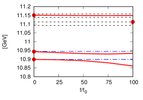
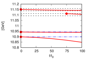
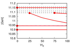
Figure 9: (Color online) Bound and resonant states of the hidden-bottom molecules with various coupling constants $f$ for $J^{P}=1/2^{-}$, using the OPEP and one of the three $5q$ potentials derived from the configuration (i) $(S_{b\bar{b}},S_{3q})=(0,1/2)$, (ii) $(1,1/2)$, or (iii) $(1,3/2)$. The horizontal axis shows the ratio $f/f_{0}$, where $f_{0}$ is the reference value defined in Sec. III.1. Solid line shows the obtained state. Filled circle is the starting point where the states appear. Dashed lines are the $B\Sigma_{\rm b}$, $B\Sigma^{\ast}_{\rm b}$, $B^{\ast}\Sigma_{\rm b}$, and $B^{\ast}\Sigma^{\ast}_{\rm b}$ thresholds. Dot-dashed lines are the $B\Lambda_{\rm b}$ and $B^{\ast}\Lambda_{\rm b}$ thresholds.

$J^{P}=1/2^{-}$

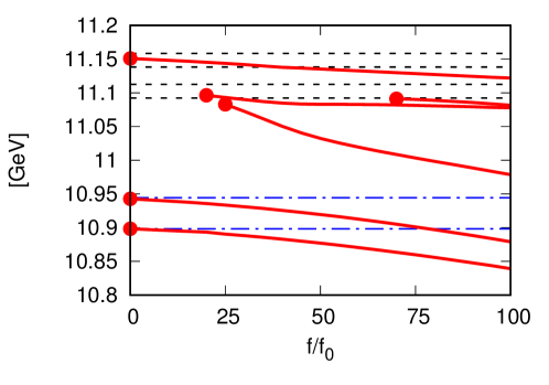
Figure 10: The same as Fig. 9 for the bound and resonant states of the hidden-bottom molecules for $J^{P}=1/2^{-}$ using the OPEP and the sum of the three $5q$ potentials.

$J^{P}=3/2^{-}$
(i) $(S_{b\bar{b}},S_{3q})=(0,\frac{3}{2})$	(ii) $(S_{b\bar{b}},S_{3q})=(1,\frac{1}{2})$	(iii) $(S_{b\bar{b}},S_{3q})=(1,\frac{3}{2})$

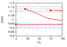
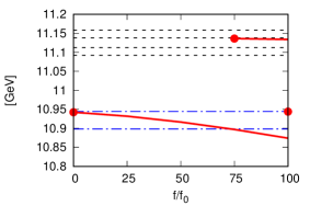
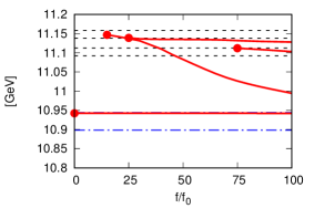
Figure 11: (Color online) The same as Fig. 9 for the bound and resonant states of the hidden-bottom molecules for $J^{P}=3/2^{-}$ using the OPEP and one of the three $5q$ potentials derived from the configuration (i) $(S_{b\bar{b}},S_{3q})=(0,3/2)$, (ii) $(1,1/2)$, or (iii) $(1,3/2)$.

$J^{P}=3/2^{-}$

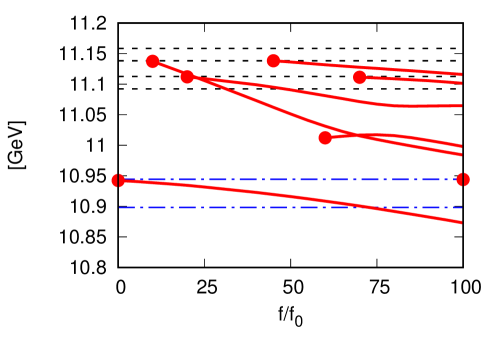
Figure 12: (Color online) The same as Fig. 9 for the bound and resonant states of the hidden-bottom molecules for $J^{P}=3/2^{-}$ using the OPEP and the sum of the three $5q$ potentials.

$J^{P}=5/2^{-}$

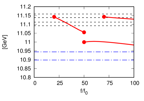
Figure 13: (Color online) The same as Fig. 9 for the resonant states of the hidden-bottom molecules for $J^{P}=5/2^{-}$ using the OPEP and the $5q$ potential from the configuration $(S_{b\bar{b}},S_{3q})=(1,\frac{3}{2})$.

Table 11: Energy spectra of the hidden-bottom molecules for $J^{P}=1/2^{-}$ using the OPEP and the $5q$ potential from the configuration (i) $(S_{b\bar{b}},S_{3q})=(0,1/2)$. The energy $E$ and half decay width $\Gamma/2$ in the various coupling constants $f/f_{0}$ are shown. The third row is for the point, where the state appears. The fourth, fifth, sixth and seventh rows show the obtained values with $f=25f_{0}$, $50f_{0}$, $75f_{0}$, and $100f_{0}$, respectively. The values are given in units of MeV. The lowest threshold $B\Lambda_{\rm b}$ is at 10898.51 MeV, and the state whose energy is lower than the threshold is a bound state.

(i) $(0,1/2)$	$f/f_{0}$	0	25	50	75	100
	$E$ [MeV]	11151	11150	11149	11149	11149
	$\Gamma/2$ [MeV]	2.01	3.05	4.25	5.32	6.08
	$f/f_{0}$	100	25	50	75	100
	$E$ [MeV]	11113	—	—	—	11113
	$\Gamma/2$ [MeV]	6.43	—	—	—	6.43
	$f/f_{0}$	0	25	50	75	100
	$E$ [MeV]	10943	10937	10932	10929	10933
	$\Gamma/2$ [MeV]	1.80$\times 10^{-2}$	0.55	2.92	7.13	7.89
	$f/f_{0}$	0	25	50	75	100
	$E$ [MeV]	10898	10897	10891	10879	10861
	$\Gamma/2$ [MeV]	—	—	—	—	—

Table 12: The same as Table 11 for the energy spectra of the hidden-bottom molecules for $J^{P}=1/2^{-}$ using the OPEP and the $5q$ potential from the configuration (ii) $(S_{b\bar{b}},S_{3q})=(1,1/2)$.

(ii) $(1,1/2)$	$f/f_{0}$	0	25	50	75	100
	$E$ [MeV]	11151	11147	11145	11143	11142
	$\Gamma/2$ [MeV]	2.01	1.75	2.76	4.22	5.52
	$f/f_{0}$	75	25	50	75	100
	$E$ [MeV]	11112	—	—	11112	11106
	$\Gamma/2$ [MeV]	7.68	—	—	7.68	5.25
	$f/f_{0}$	0	25	50	75	100
	$E$ [MeV]	10943	10941	10941	10940	10939
	$\Gamma/2$ [MeV]	1.80$\times 10^{-2}$	0.19	0.31	0.33	0.22
	$f/f_{0}$	0	25	50	75	100
	$E$ [MeV]	10898	10893	10882	10867	10848
	$\Gamma/2$ [MeV]	—	—	—	—	—

Table 13: The same as Table 11 for the energy spectra of the hidden-bottom molecules for $J^{P}=1/2^{-}$ using the OPEP and the $5q$ potential from the configuration (iii) $(S_{b\bar{b}},S_{3q})=(1,3/2)$.

(iii) $(1,3/2)$	$f/f_{0}$	0	25	50	75	100
	$E$ [MeV]	11151	11151	11151	11151	11151
	$\Gamma/2$ [MeV]	2.01	2.63	2.89	2.92	2.91
	$f/f_{0}$	75	25	50	75	100
	$E$ [MeV]	11090	—	—	11090	11082
	$\Gamma/2$ [MeV]	0.37	—	—	0.37	0.30
	$f/f_{0}$	25	25	50	75	100
	$E$ [MeV]	11089	11089	11036	11002	10976
	$\Gamma/2$ [MeV]	29.54	29.54	26.93	12.38	4.35
	$f/f_{0}$	0	25	50	75	100
	$E$ [MeV]	10943	10943	10943	10943	10942
	$\Gamma/2$ [MeV]	1.80$\times 10^{-2}$	0.13	0.13	0.13	0.17
	$f/f_{0}$	0	25	50	75	100
	$E$ [MeV]	10898	10898	10898	10898	10898
	$\Gamma/2$ [MeV]	—	—	—	—	—

Table 14: The same as Table 11 for the energy spectra of the hidden-bottom molecules for $J^{P}=1/2^{-}$ using the OPEP and the sum of the three $5q$ potentials.

SUM	$f/f_{0}$	0	25	50	75	100
	$E$ [MeV]	11151	11144	11135	11129	11122
	$\Gamma/2$ [MeV]	2.01	2.67	0.60	0.58	0.60
	$f/f_{0}$	70	25	50	75	100
	$E$ [MeV]	11091	—	—	11090	11082
	$\Gamma/2$ [MeV]	0.36	—	—	0.44	0.75
	$f/f_{0}$	20	25	50	75	100
	$E$ [MeV]	11096	11093	11083	11081	11078
	$\Gamma/2$ [MeV]	44.69	11.35	14.15	31.45	39.32
	$f/f_{0}$	25	25	50	75	100
	$E$ [MeV]	11083	11083	11033	11003	10979
	$\Gamma/2$ [MeV]	78.77	78.77	40.76	14.49	4.03
	$f/f_{0}$	0	25	50	75	100
	$E$ [MeV]	10943	10934	10920	10901	10879
	$\Gamma/2$ [MeV]	1.80$\times 10^{-2}$	1.91$\times 10^{-2}$	5.80$\times 10^{-2}$	0.12	—
	$f/f_{0}$	0	25	50	75	100
	$E$ [MeV]	10898	10891	10877	10860	10839
	$\Gamma/2$ [MeV]	—	—	—	—	—

Table 15: The same as Table 11 for the energy spectra of the hidden-bottom molecules for $J^{P}=3/2^{-}$ using the OPEP and the $5q$ potential from the configuration (i) $(S_{b\bar{b}},S_{3q})=(0,3/2)$.

(i) $(0,3/2)$	$f/f_{0}$	75	25	50	75	100
	$E$ [MeV]	11112	—	—	11112	11107
	$\Gamma/2$ [MeV]	1.13	—	—	1.13	1.13
	$f/f_{0}$	20	25	50	75	100
	$E$ [MeV]	11129	11120	11062	11011	10987
	$\Gamma/2$ [MeV]	57.15	59.69	64.94	34.53	16.76
	$f/f_{0}$	0	25	50	75	100
	$E$ [MeV]	10942	10942	10942	10942	10941
	$\Gamma/2$ [MeV]	3.08$\times 10^{-2}$	0.15	0.17	0.16	0.23

Table 16: The same as Table 11 for the energy spectra of the hidden-bottom molecules for $J^{P}=3/2^{-}$ using the OPEP and the $5q$ potential from the configuration (ii) $(S_{b\bar{b}},S_{3q})=(1,1/2)$.

(ii) $(1,1/2)$	$f/f_{0}$	75	25	50	75	100
	$E$ [MeV]	11136	—	—	11136	11134
	$\Gamma/2$ [MeV]	19.45	—	—	19.45	11.86
	$f/f_{0}$	100	25	50	75	100
	$E$ [MeV]	10944	—	—	—	10944
	$\Gamma/2$ [MeV]	0.11	—	—	—	0.11
	$f/f_{0}$	0	25	50	75	100
	$E$ [MeV]	10942	10932	10917	10897	10874
	$\Gamma/2$ [MeV]	3.08$\times 10^{-2}$	0.13	0.11	—	—

Table 17: The same as Table 11 for the energy spectra of the hidden-bottom molecules for $J^{P}=3/2^{-}$ using the OPEP and the $5q$ potential from the configuration (iii) $(S_{b\bar{b}},S_{3q})=(1,3/2)$.

(iii) $(1,3/2)$	$f/f_{0}$	25	25	50	75	100
	$E$ [MeV]	11139	11139	11135	11132	11128
	$\Gamma/2$ [MeV]	22.58	22.58	16.00	11.53	12.61
	$f/f_{0}$	75	25	50	75	100
	$E$ [MeV]	11112	—	—	11112	11103
	$\Gamma/2$ [MeV]	1.91	—	—	1.91	1.15
	$f/f_{0}$	15	25	50	75	100
	$E$ [MeV]	11147	11137	11083	11027	10995
	$\Gamma/2$ [MeV]	47.21	45.51	40.07	28.14	11.19
	$f/f_{0}$	0	25	50	75	100
	$E$ [MeV]	10942	10942	10942	10942	10942
	$\Gamma/2$ [MeV]	3.08$\times 10^{-2}$	8.92$\times 10^{-3}$	1.01$\times 10^{-2}$	1.21$\times 10^{-2}$	1.68$\times 10^{-2}$

Table 18: The same as Table 11 for the energy spectra of the hidden-bottom molecules for $J^{P}=3/2^{-}$ using the OPEP and the sum of the three $5q$ potentials.

SUM	$f/f_{0}$	45	25	50	75	100
	$E$ [MeV]	11138	—	11136	11126	11116
	$\Gamma/2$ [MeV]	5.13	—	5.71	3.78	1.94
	$f/f_{0}$	70	25	50	75	100
	$E$ [MeV]	11111	—	—	11110	11101
	$\Gamma/2$ [MeV]	0.27	—	—	0.35	0.70
	$f/f_{0}$	20	25	50	75	100
	$E$ [MeV]	11112	11109	11091	11067	11065
	$\Gamma/2$ [MeV]	4.40	5.57	11.82	28.88	51.60
	$f/f_{0}$	60	25	50	75	100
	$E$ [MeV]	11012	—	—	11017	10998
	$\Gamma/2$ [MeV]	53.76	—	—	37.95	10.85

Table 19: Continued from Table 18.

SUM	$f/f_{0}$	10	25	50	75	100
	$E$ [MeV]	11137	11106	11051	11010	10984
	$\Gamma/2$ [MeV]	52.77	58.70	54.22	29.71	12.94
	$f/f_{0}$	100	25	50	75	100
	$E$ [MeV]	10944	—	—	—	10944
	$\Gamma/2$ [MeV]	4.70$\times 10^{-3}$	—	—	—	4.70$\times 10^{-3}$
	$f/f_{0}$	0	25	50	75	100
	$E$ [MeV]	10942	10932	10916	10896	10873
	$\Gamma/2$ [MeV]	3.08$\times 10^{-2}$	7.83$\times 10^{-3}$	1.97$\times 10^{-3}$	—	—

Table 20: The same as Table 11 for the energy spectra of the hidden-bottom molecules for $J^{P}=5/2^{-}$ using the OPEP and the $5q$ potential from the configuration $(S_{b\bar{b}},S_{3q})=(1,3/2)$.

$(1,3/2)$	$f/f_{0}$	70	25	50	75	100
	$E$ [MeV]	11142.84	—	—	11139.85	11129.35
	$\Gamma/2$ [MeV]	15.89	—	—	12.66	5.15
	$f/f_{0}$	20	25	50	75	100
	$E$ [MeV]	11142.42	11128.79	11055.16	—	—
	$\Gamma/2$ [MeV]	123.11	125.94	153.98	—	—
	$f/f_{0}$	50	25	50	75	100
	$E$ [MeV]	10999.46	—	10999.46	10998.89	10983.33
	$\Gamma/2$ [MeV]	71.82	—	71.82	36.75	17.97

IV Summary

In this paper, we have studied hidden-charm and hidden-bottom pentaquark states. Since the observed $P_{c}$’s are in the open-charm threshold region, we have performed a coupled channel analyses with various meson-baryon states which may generate bound and resonant states. In such an analysis, the hadronic interaction is the most important input. At long distances, we employ the one-pion exchange potential which is best known among various hadron interactions. As discussed and emphasized in many works, the OPEP provides attraction when the tensor force is at work through the $SD$ coupled channels. This is crucially important for the formation of the exotic pentaquark states.

Contrary, for short range interaction which is far less known, we inferred from a recent quark cluster model analysis pointing out the importance of the colorful $5q$ configurations. We have included these $5q$ configurations in the coupled channel problems as one-particle states. By eliminating them we have derived an effective interaction at short distances. Since all the expected $5q$ states locate above the meson-baryon threshold region, the resulting effective interaction is attractive, which can be another driving force for the generation of the pentaquark states. The coupling of this interaction to various meson-baryon channels is estimated by the spectroscopic factor. Therefore, our model contains essentially only one parameter which is the overall strength of the short range interaction $f$. Then results are shown for various $f$ up to the maximum strength which we expect from our current knowledge of the hadron interaction.

For the charm sector, when the $5q$ interaction is turned on, bound and resonant states are generated for various spins, $1/2^{-}$, $3/2^{-}$, and $5/2^{-}$. Among them, $3/2^{-}$ state with mass around 4460 MeV and width around 25 MeV (see Table 7) is a candidate of the observed $P_{c}$, though the spin parity identification is not the suggested one. Therefore, in this paper, we have further concentrated on the mechanism how the pentaquark states are generated.

For the bottom sector, due to the suppression of the kinetic energy, we have seen abundant pentaquark states even only by the OPEP. These are the rather robust predictions of our analysis. Therefore, with possible further attractions from the short range interaction, we indeed expect many exotic pentaquark states. In this way, we suggest experimental analysis to search for further states in the bottom region.

We have also compared our present analysis with the previous quark cluster model one. We have found similarities between them, and therefore, our approach provides a good method to make physical interpretations for the results of the quark cluster model.

In the present analysis we have studied negative parity states dominated by the $S$-wave configurations of open charm channels. For more complete analysis, it is needed to include hidden-charm channels such as $J/\psi p$. In the case of the $Z_{c}(3900)$, the importance of the mixing of $\bar{D}D^{\ast}-J/\psi\pi$ has been indicated by a lattice QCD simulation Ikeda:2016zwx . It is also interesting to study positive parity states. For this, we need $P$-wave excitations for both meson-baryon and for 5q states. Moreover, couplings to such as $\bar{D}\Lambda_{\rm c}(2595)$ channel can be important because of their very close threshold to the $\bar{D}\Lambda_{\rm c}(2595)$ threshold, and to the reported $P_{\rm c}(4450)$ state Burns:2015dwa . As discussed in Ref. Geng:2017hxc , such a coupling may show up a unique feature of the universal phenomena caused by the almost on-shell pion decaying from the $\Lambda_{c}(2595)$. All these issues may be studied as interesting future investigations.

Appendix A Explicit form of the one-pion exchange potential

The OPEP is given by the effective Lagrangians in Eqs. (18) and (25). We use the static approximation where the energy transfer is neglected as compared to the momentum transfer. The OPEP for isospon $I=1/2$ is obtained by

$$V^{\pi}_{\bar{D}^{\ast}\Sigma_{\rm c}-\bar{D}\Lambda_{\rm c}}(r)=-\frac{gg_{4}}{3\sqrt{2}f^{2}_{\pi}}\left[\vec{\varepsilon}\,^{\dagger}\cdot\vec{\sigma}C(r)+S_{\varepsilon{\sigma}}(\hat{r})T(r)\right],$$ (55)

$$V^{\pi}_{\bar{D}^{\ast}\Sigma^{\ast}_{\rm c}-\bar{D}\Lambda_{\rm c}}(r)=\frac{gg_{4}}{\sqrt{6}f^{2}_{\pi}}\left[\vec{\varepsilon}\,^{\dagger}\cdot\vec{\bar{\Sigma}}C(r)+S_{\varepsilon\bar{\Sigma}}(\hat{r})T(r)\right],$$ (56)

$$V^{\pi}_{\bar{D}\Sigma_{\rm c}-\bar{D}^{\ast}\Lambda_{\rm c}}(r)=-\frac{gg_{4}}{3\sqrt{2}f^{2}_{\pi}}\left[\vec{\varepsilon}\cdot\vec{\sigma}C(r)+S_{\varepsilon{\sigma}}(\hat{r})T(r)\right],$$ (57)

$$V^{\pi}_{\bar{D}\Sigma^{\ast}_{\rm c}-\bar{D}^{\ast}\Lambda_{\rm c}}(r)=\frac{gg_{4}}{\sqrt{6}f^{2}_{\pi}}\left[\vec{\varepsilon}\cdot\vec{\bar{\Sigma}}C(r)+S_{\varepsilon\bar{\Sigma}}(\hat{r})T(r)\right],$$ (58)

$$V^{\pi}_{\bar{D}^{\ast}\Sigma_{\rm c}-\bar{D}^{\ast}\Lambda_{\rm c}}(r)=-\frac{gg_{4}}{3\sqrt{2}f^{2}_{\pi}}\left[\vec{S}\cdot\vec{\sigma}C(r)+S_{S{\sigma}}(\hat{r})T(r)\right],$$ (59)

$$V^{\pi}_{\bar{D}^{\ast}\Sigma^{\ast}_{\rm c}-\bar{D}^{\ast}\Lambda_{\rm c}}(r)=\frac{gg_{4}}{\sqrt{6}f^{2}_{\pi}}\left[\vec{S}\cdot\vec{\bar{\Sigma}}^{\dagger}C(r)+S_{S\bar{\Sigma}}(\hat{r})T(r)\right],$$ (60)

$$V^{\pi}_{\bar{D}^{\ast}\Sigma_{\rm c}-\bar{D}\Sigma_{\rm c}}(r)=\frac{gg_{1}}{3f^{2}_{\pi}}\left[\vec{\varepsilon}\,^{\dagger}\cdot\vec{\sigma}C(r)+S_{\varepsilon{\sigma}}(\hat{r})T(r)\right],$$ (61)

$$V^{\pi}_{\bar{D}^{\ast}\Sigma^{\ast}_{\rm c}-\bar{D}\Sigma_{\rm c}}(r)=\frac{gg_{1}}{2\sqrt{3}f^{2}_{\pi}}\left[\vec{\varepsilon}\,^{\dagger}\cdot\vec{\bar{\Sigma}}\,^{\dagger}C(r)+S_{\varepsilon\bar{\Sigma}}(\hat{r})T(r)\right],$$ (62)

$$V^{\pi}_{\bar{D}^{\ast}\Sigma_{\rm c}-\bar{D}\Sigma^{\ast}_{\rm c}}(r)=\frac{gg_{1}}{2\sqrt{3}f^{2}_{\pi}}\left[\vec{\varepsilon}\,^{\dagger}\cdot\vec{\bar{\Sigma}}C(r)+S_{\varepsilon\bar{\Sigma}}(\hat{r})T(r)\right],$$ (63)

$$V^{\pi}_{\bar{D}^{\ast}\Sigma^{\ast}_{\rm c}-\bar{D}\Sigma^{\ast}_{\rm c}}(r)=\frac{gg_{1}}{3f^{2}_{\pi}}\left[\vec{\varepsilon}\,^{\dagger}\cdot\vec{\Sigma}C(r)+S_{\varepsilon\Sigma}(\hat{r})T(r)\right],$$ (64)

$$V^{\pi}_{\bar{D}^{\ast}\Sigma_{\rm c}-\bar{D}^{\ast}\Sigma_{\rm c}}(r)=-\frac{gg_{1}}{3f^{2}_{\pi}}\left[\vec{S}\cdot\vec{\sigma}C(r)+S_{S\sigma}(\hat{r})T(r)\right],$$ (65)

$$V^{\pi}_{\bar{D}^{\ast}\Sigma^{\ast}_{\rm c}-\bar{D}^{\ast}\Sigma_{\rm c}}(r)=\frac{gg_{1}}{2\sqrt{3}f^{2}_{\pi}}\left[\vec{S}\cdot\vec{\bar{\Sigma}}^{\dagger}C(r)+S_{S\bar{\Sigma}}(\hat{r})T(r)\right],$$ (66)

$$V^{\pi}_{\bar{D}^{\ast}\Sigma^{\ast}_{\rm c}-\bar{D}^{\ast}\Sigma^{\ast}_{\rm c}}(r)=\frac{gg_{1}}{3f^{2}_{\pi}}\left[\vec{S}\cdot\vec{\Sigma}C(r)+S_{S\Sigma}(\hat{r})T(r)\right].$$ (67)

The tensor operator $S_{{\cal O}_{\bar{D}}{\cal O}_{Y_{c}}}(\hat{r})$ is defined by $S_{{\cal O}_{\bar{D}}{\cal O}_{Y_{c}}}(\hat{r})=3\vec{\cal O}_{\bar{D}}\cdot\hat{r}\vec{\cal O}_{Y_{c}}\cdot\hat{r}-\vec{\cal O}_{\bar{D}}\cdot\vec{\cal O}_{Y_{c}}$ with the spin operators ${\cal O}_{\bar{D}}=\varepsilon,S$ for the meson vertex and ${\cal O}_{Y_{c}}=\sigma,\bar{\Sigma},\Sigma$ for the baryon vertex. The polarization vector is defined by $\vec{\varepsilon}\,^{(\pm)}=(\mp 1/\sqrt{2},\pm i/\sqrt{2},0)$ and $\vec{\varepsilon}\,^{(0)}=(0,0,1)$. The spin-one operator is $\vec{S}=i\vec{\varepsilon}\times\vec{\varepsilon}\,^{\dagger}$, $\vec{\sigma}$ is the Pauli matrices, $\bar{\Sigma}^{\mu}$ is given by

$$\bar{\Sigma}^{\mu}=\left(\begin{array}[]{cccc}\vec{\varepsilon}\,^{(+)}&\sqrt{2/3}\vec{\varepsilon}\,^{(0)}&\sqrt{1/3}\vec{\varepsilon}\,^{(-)}&0\\ 0&\sqrt{1/3}\vec{\varepsilon}\,^{(+)}&\sqrt{2/3}\vec{\varepsilon}\,^{(0)}&\vec{\varepsilon}\,^{(-)}\\ \end{array}\right)^{\mu},$$ (70)

and $\vec{\Sigma}$ is defined by $\vec{\Sigma}=\frac{3}{2}i\vec{\bar{\Sigma}}\times\vec{\bar{\Sigma}}\,^{\dagger}$. The functions $C(r)$ and $T(r)$ are given by

$$C(r)=\int\frac{d^{3}q}{(2\pi)^{3}}\frac{m^{2}_{\pi}}{\vec{q}\,^{2}+m^{2}_{\pi}}e^{i\vec{q}\cdot\vec{r}}F(\Lambda,\vec{q}\,),$$ (71)

$$S_{\cal O}(\hat{r})T(r)=\int\frac{d^{3}q}{(2\pi)^{3}}\frac{-\vec{q}\,^{2}}{\vec{q}\,^{2}+m^{2}_{\pi}}S_{\cal O}(\hat{q})e^{i\vec{q}\cdot\vec{r}}F(\Lambda,\vec{q}\,),$$ (72)

with the form factor (33). We note that the contact term of the central force (71) is neglected as discussed in the nucleon-nucleon meson exchange potential Machleidt:1987hj .

The kinetic terms are give by

$$K_{i}=-\frac{1}{2\mu_{i}}\triangle_{L_{i}}+\Delta m_{i},$$ (73)

of the channel $i$ given in Table 1. We define the reduced mass $\mu_{i}=m_{M_{i}}m_{B_{i}}/(m_{M_{i}}+m_{B_{i}})$ of the meson $M_{i}(=\bar{D},\bar{D}^{\ast})$ and baryon $B_{i}(=\Lambda_{\rm c},\Sigma_{\rm c},\Sigma^{\ast}_{\rm c})$, $\triangle_{L_{i}}=\partial^{2}/\partial r^{2}+(2/r)\partial/\partial r+L_{i}(L_{i}+1)/r^{2}$ with the orbital angular momentum $L_{i}$, and $\Delta m_{i}=(m_{M_{i}}+m_{B_{i}})-(m_{\bar{D}}+m_{\Lambda_{\rm c}})$.

Appendix B Computation of spectroscopic factor

The wave function of the hidden-charm five-quark ($5q$) state is written by three light quarks $uud$ and charm and anti-charm quarks $c\bar{c}$ as $\Ket{5q}=\Ket{u(1)u(2)d(3)c(4)\bar{c}(5)}$ with the particle number assignment. The wave function can also be decomposed into various meson-baron components as

$$\Ket{5q} =a\Ket{\left(u(1)u(2)c(4)\right)^{\frac{1}{2}}\left(d(3)\bar{c}(5)\right)^{0}}+\dots\equiv a\Ket{\Sigma^{++}_{\rm c}\bar{D}^{-}}+\dots,$$ (74)

where $a$ is the definition of the spectroscopic factor Hosaka:2004bn , and the superscript is the total spin of three quarks or quark-antiquark. Assuming that $\Ket{\left(u(1)u(2)c(4)\right)^{\frac{1}{2}}\left(d(3)\bar{c}(5)\right)^{0}}$ is exactly the same as the hadronic wave function of $\Sigma^{++}_{\rm c}\bar{D}^{-}$, the spectroscopic factor for the $\Sigma^{++}_{\rm c}\bar{D}^{-}$ channel is obtained by the overlap

$$a =\Braket{\Sigma^{++}_{\rm c}\bar{D}^{-}}{5q}.$$ (75)

In this Appendix, we will focus on the color-flavor-spin wave function of the $5q$ states, in which the $uud$ ($3q$) system and the $c\bar{c}$ system are both in the color octet, and the total color wave function is in the color-singlet. Moreover, the light quarks are assumed to be the $S-$wave state, that is, the orbital wave function is totally symmetric. Since the total wave function of the three light quarks must be antisymmetric, it is represented in Young tableaux as

$$\hbox{}\vbox{\vbox{\offinterlineskip\vbox{\hrule height=0.3pt\hbox{\vrule height=8.74669pt,width=0.3pt,depth=2.18663pt\hbox to10.93333pt{\hfil}\vrule height=8.74669pt,width=0.3pt,depth=2.18663pt} \hrule height=0.3pt}\vspace{-\y@linethick} \vbox{\hrule height=0.3pt\hbox{\vrule height=8.74669pt,width=0.3pt,depth=2.18663pt\hbox to10.93333pt{\hfil}\vrule height=8.74669pt,width=0.3pt,depth=2.18663pt} \hrule height=0.3pt}\vspace{-\y@linethick} \vbox{\hrule height=0.3pt\hbox{\vrule height=8.74669pt,width=0.3pt,depth=2.18663pt\hbox to10.93333pt{\hfil}\vrule height=8.74669pt,width=0.3pt,depth=2.18663pt} \hrule height=0.3pt}\vspace{-\y@linethick} }}\,\raisebox{-19.91692pt}{$csfo$}\;\;=\;\;\hbox{}\vbox{\vbox{\offinterlineskip\vbox{\hrule height=0.3pt\hbox{\vrule height=8.74669pt,width=0.3pt,depth=2.18663pt\hbox to10.93333pt{\hfil}\vrule height=8.74669pt,width=0.3pt,depth=2.18663pt} \hrule height=0.3pt}\vspace{-\y@linethick} \vbox{\hrule height=0.3pt\hbox{\vrule height=8.74669pt,width=0.3pt,depth=2.18663pt\hbox to10.93333pt{\hfil}\vrule height=8.74669pt,width=0.3pt,depth=2.18663pt} \hrule height=0.3pt}\vspace{-\y@linethick} \vbox{\hrule height=0.3pt\hbox{\vrule height=8.74669pt,width=0.3pt,depth=2.18663pt\hbox to10.93333pt{\hfil}\vrule height=8.74669pt,width=0.3pt,depth=2.18663pt} \hrule height=0.3pt}\vspace{-\y@linethick} }}\,\raisebox{-19.91692pt}{$csf$}\;\;\cdot\;\;\hbox{}\vbox{\vbox{\offinterlineskip\vbox{\hrule height=0.3pt\hbox{\vrule height=8.74669pt,width=0.3pt,depth=2.18663pt\hbox to10.93333pt{\hfil}\vrule height=8.74669pt,width=0.3pt,depth=2.18663pt\hbox to10.93333pt{\hfil}\vrule height=8.74669pt,width=0.3pt,depth=2.18663pt\hbox to10.93333pt{\hfil}\vrule height=8.74669pt,width=0.3pt,depth=2.18663pt} \hrule height=0.3pt}\vspace{-\y@linethick} }}\,\raisebox{-8.53581pt}{$o$}\;\;\;\;,$$ (76)

where the subscripts $c$, $s$, $f$, and $o$ denote color, spin, flavor, and orbital wave functions, respectively. The center dot “ $\cdot$ ” denotes the inner product of wave functions in different functional space.

The $csf$ wave function is decomposed into color and spin-flavor parts. In the Young tableaux with the particle number assignment, one obtains (see, e.g., Ref. Chen:2002gd )

  $$1 2 3 csf =\frac{1}{\sqrt{2}}\left(\;\hbox{}\vbox{\vbox{\offinterlineskip \vbox{ \hrule height=0.3pt\hbox{\vrule height=8.74669pt,width=0.3pt,depth=2.18663pt\hbox to10.93333pt{\hfil$1$\hfil}\vrule height=8.74669pt,width=0.3pt,depth=2.18663pt\hbox to10.93333pt{\hfil$2$\hfil}\vrule height=8.74669pt,width=0.3pt,depth=2.18663pt}\hrule height=0.3pt}\vspace{-\y@linethick} \vbox{ \hrule height=0.3pt\hbox{\vrule height=8.74669pt,width=0.3pt,depth=2.18663pt\hbox to10.93333pt{\hfil$3$\hfil}\vrule height=8.74669pt,width=0.3pt,depth=2.18663pt} \hrule height=0.3pt}\vspace{-\y@linethick} }}\,\raisebox{-14.22636pt}{$c$}\cdot\,\hbox{}\vbox{\vbox{\offinterlineskip \vbox{ \hrule height=0.3pt\hbox{\vrule height=8.74669pt,width=0.3pt,depth=2.18663pt\hbox to10.93333pt{\hfil$1$\hfil}\vrule height=8.74669pt,width=0.3pt,depth=2.18663pt\hbox to10.93333pt{\hfil$3$\hfil}\vrule height=8.74669pt,width=0.3pt,depth=2.18663pt}\hrule height=0.3pt}\vspace{-\y@linethick} \vbox{ \hrule height=0.3pt\hbox{\vrule height=8.74669pt,width=0.3pt,depth=2.18663pt\hbox to10.93333pt{\hfil$2$\hfil}\vrule height=8.74669pt,width=0.3pt,depth=2.18663pt} \hrule height=0.3pt}\vspace{-\y@linethick} }}\,\raisebox{-14.22636pt}{$sf$}-\hbox{}\vbox{\vbox{\offinterlineskip \vbox{ \hrule height=0.3pt\hbox{\vrule height=8.74669pt,width=0.3pt,depth=2.18663pt\hbox to10.93333pt{\hfil$1$\hfil}\vrule height=8.74669pt,width=0.3pt,depth=2.18663pt\hbox to10.93333pt{\hfil$3$\hfil}\vrule height=8.74669pt,width=0.3pt,depth=2.18663pt}\hrule height=0.3pt}\vspace{-\y@linethick} \vbox{ \hrule height=0.3pt\hbox{\vrule height=8.74669pt,width=0.3pt,depth=2.18663pt\hbox to10.93333pt{\hfil$2$\hfil}\vrule height=8.74669pt,width=0.3pt,depth=2.18663pt} \hrule height=0.3pt}\vspace{-\y@linethick} }}\,\raisebox{-14.22636pt}{$c$}\cdot\,\hbox{}\vbox{\vbox{\offinterlineskip \vbox{ \hrule height=0.3pt\hbox{\vrule height=8.74669pt,width=0.3pt,depth=2.18663pt\hbox to10.93333pt{\hfil$1$\hfil}\vrule height=8.74669pt,width=0.3pt,depth=2.18663pt\hbox to10.93333pt{\hfil$2$\hfil}\vrule height=8.74669pt,width=0.3pt,depth=2.18663pt}\hrule height=0.3pt}\vspace{-\y@linethick} \vbox{ \hrule height=0.3pt\hbox{\vrule height=8.74669pt,width=0.3pt,depth=2.18663pt\hbox to10.93333pt{\hfil$3$\hfil}\vrule height=8.74669pt,width=0.3pt,depth=2.18663pt} \hrule height=0.3pt}\vspace{-\y@linethick} }}\,\raisebox{-14.22636pt}{$sf$}\;\right).$$           (77)

In Eq. (77), the color wave functions in the first and second terms have different types of symmetry for exchanges,

$$\hbox{}\vbox{\vbox{\offinterlineskip \vbox{ \hrule height=0.3pt\hbox{\vrule height=8.74669pt,width=0.3pt,depth=2.18663pt\hbox to10.93333pt{\hfil$1$\hfil}\vrule height=8.74669pt,width=0.3pt,depth=2.18663pt\hbox to10.93333pt{\hfil$2$\hfil}\vrule height=8.74669pt,width=0.3pt,depth=2.18663pt}\hrule height=0.3pt}\vspace{-\y@linethick} \vbox{ \hrule height=0.3pt\hbox{\vrule height=8.74669pt,width=0.3pt,depth=2.18663pt\hbox to10.93333pt{\hfil$3$\hfil}\vrule height=8.74669pt,width=0.3pt,depth=2.18663pt} \hrule height=0.3pt}\vspace{-\y@linethick} }}\,\raisebox{-14.22636pt}{$c$}\equiv([21]1)_{c},$$ (78)

and

$$\hbox{}\vbox{\vbox{\offinterlineskip \vbox{ \hrule height=0.3pt\hbox{\vrule height=8.74669pt,width=0.3pt,depth=2.18663pt\hbox to10.93333pt{\hfil$1$\hfil}\vrule height=8.74669pt,width=0.3pt,depth=2.18663pt\hbox to10.93333pt{\hfil$3$\hfil}\vrule height=8.74669pt,width=0.3pt,depth=2.18663pt}\hrule height=0.3pt}\vspace{-\y@linethick} \vbox{ \hrule height=0.3pt\hbox{\vrule height=8.74669pt,width=0.3pt,depth=2.18663pt\hbox to10.93333pt{\hfil$2$\hfil}\vrule height=8.74669pt,width=0.3pt,depth=2.18663pt} \hrule height=0.3pt}\vspace{-\y@linethick} }}\,\raisebox{-14.22636pt}{$c$}\equiv([21]2)_{c},$$ (79)

where $c$ means that the permutations $[21]1$ and $[21]2$ are performed in the color space. The difference between (78) and (79) lies in the permutation symmetry for exchange: in Eq. (78), particles 1 and 2 are symmetric for exchange, while particle 1 and 2 are antisymmetric in Eq. (79). The wave function of the $5q$ state is given by the direct product between the $3q$ and $c\bar{c}$ wave functions. For this reason, the color part of the total $5q$ state wave function also contains these two permutation symmetries, the $([21]1)_{c}$ and the $([21]2)_{c}$, and so in the calculations of the spectroscopic factors, both permutations will be considered.

Since the spin of the $c\bar{c}$ pair can be $S_{c\bar{c}}=0$ or 1, there are two $5q$ state wave functions denoted with $\Ket{5q,\mathbb{S_{c\bar{c}}=0}}$ and $\Ket{5q,\mathbb{S_{c\bar{c}}=1}}$. In the case of $S_{c\bar{c}}=0$, the $c\bar{c}$ wave function $\psi^{s=0}_{c\bar{c}}$ is

$$\psi_{c\bar{c}}^{s=0}\sim\hbox{}\vbox{\vbox{\offinterlineskip \vbox{ \hrule height=0.3pt\hbox{\vrule height=8.74669pt,width=0.3pt,depth=2.18663pt\hbox to10.93333pt{\hfil$5$\hfil}\vrule height=8.74669pt,width=0.3pt,depth=2.18663pt\hbox to10.93333pt{\hfil$4$\hfil}\vrule height=8.74669pt,width=0.3pt,depth=2.18663pt}\hrule height=0.3pt}\vspace{-\y@linethick} \vbox{ \hrule height=0.3pt\hbox{\vrule height=8.74669pt,width=0.3pt,depth=2.18663pt\hbox to10.93333pt{\hfil$5$\hfil}\vrule height=8.74669pt,width=0.3pt,depth=2.18663pt} \hrule height=0.3pt}\vspace{-\y@linethick} }}\,\raisebox{-14.22636pt}{$c$}\;\;\cdot\;\;\hbox{}\vbox{\vbox{\offinterlineskip \vbox{ \hrule height=0.3pt\hbox{\vrule height=8.74669pt,width=0.3pt,depth=2.18663pt\hbox to10.93333pt{\hfil$4$\hfil}\vrule height=8.74669pt,width=0.3pt,depth=2.18663pt} \hrule height=0.3pt}\vspace{-\y@linethick} \vbox{ \hrule height=0.3pt\hbox{\vrule height=8.74669pt,width=0.3pt,depth=2.18663pt\hbox to10.93333pt{\hfil$5$\hfil}\vrule height=8.74669pt,width=0.3pt,depth=2.18663pt} \hrule height=0.3pt}\vspace{-\y@linethick} }}\,\raisebox{-14.22636pt}{$s$},$$ (80)

and the $5q$ state wave function $\Ket{5q,\mathbb{S_{c\bar{c}}=0}}$ is given by

$$\Ket{5q,\mathbb{S_{c\bar{c}}=0}}\;\sim \frac{1}{\sqrt{2}}\left(\;\hbox{}\vbox{\vbox{\offinterlineskip \vbox{ \hrule height=0.3pt\hbox{\vrule height=8.74669pt,width=0.3pt,depth=2.18663pt\hbox to10.93333pt{\hfil$1$\hfil}\vrule height=8.74669pt,width=0.3pt,depth=2.18663pt\hbox to10.93333pt{\hfil$2$\hfil}\vrule height=8.74669pt,width=0.3pt,depth=2.18663pt}\hrule height=0.3pt}\vspace{-\y@linethick} \vbox{ \hrule height=0.3pt\hbox{\vrule height=8.74669pt,width=0.3pt,depth=2.18663pt\hbox to10.93333pt{\hfil$3$\hfil}\vrule height=8.74669pt,width=0.3pt,depth=2.18663pt} \hrule height=0.3pt}\vspace{-\y@linethick} }}\,\raisebox{-14.22636pt}{$c$}\;\;\cdot\;\;\hbox{}\vbox{\vbox{\offinterlineskip \vbox{ \hrule height=0.3pt\hbox{\vrule height=8.74669pt,width=0.3pt,depth=2.18663pt\hbox to10.93333pt{\hfil$1$\hfil}\vrule height=8.74669pt,width=0.3pt,depth=2.18663pt\hbox to10.93333pt{\hfil$3$\hfil}\vrule height=8.74669pt,width=0.3pt,depth=2.18663pt}\hrule height=0.3pt}\vspace{-\y@linethick} \vbox{ \hrule height=0.3pt\hbox{\vrule height=8.74669pt,width=0.3pt,depth=2.18663pt\hbox to10.93333pt{\hfil$2$\hfil}\vrule height=8.74669pt,width=0.3pt,depth=2.18663pt} \hrule height=0.3pt}\vspace{-\y@linethick} }}\,\raisebox{-14.22636pt}{$sf$}-\hbox{}\vbox{\vbox{\offinterlineskip \vbox{ \hrule height=0.3pt\hbox{\vrule height=8.74669pt,width=0.3pt,depth=2.18663pt\hbox to10.93333pt{\hfil$1$\hfil}\vrule height=8.74669pt,width=0.3pt,depth=2.18663pt\hbox to10.93333pt{\hfil$3$\hfil}\vrule height=8.74669pt,width=0.3pt,depth=2.18663pt}\hrule height=0.3pt}\vspace{-\y@linethick} \vbox{ \hrule height=0.3pt\hbox{\vrule height=8.74669pt,width=0.3pt,depth=2.18663pt\hbox to10.93333pt{\hfil$2$\hfil}\vrule height=8.74669pt,width=0.3pt,depth=2.18663pt} \hrule height=0.3pt}\vspace{-\y@linethick} }}\,\raisebox{-14.22636pt}{$c$}\;\;\cdot\;\;\hbox{}\vbox{\vbox{\offinterlineskip \vbox{ \hrule height=0.3pt\hbox{\vrule height=8.74669pt,width=0.3pt,depth=2.18663pt\hbox to10.93333pt{\hfil$1$\hfil}\vrule height=8.74669pt,width=0.3pt,depth=2.18663pt\hbox to10.93333pt{\hfil$2$\hfil}\vrule height=8.74669pt,width=0.3pt,depth=2.18663pt}\hrule height=0.3pt}\vspace{-\y@linethick} \vbox{ \hrule height=0.3pt\hbox{\vrule height=8.74669pt,width=0.3pt,depth=2.18663pt\hbox to10.93333pt{\hfil$3$\hfil}\vrule height=8.74669pt,width=0.3pt,depth=2.18663pt} \hrule height=0.3pt}\vspace{-\y@linethick} }}\,\raisebox{-14.22636pt}{$sf$}\;\right)$$

$$\;\;\cdot\;\;\left(\;\;\;\hbox{}\vbox{\vbox{\offinterlineskip \vbox{ \hrule height=0.3pt\hbox{\vrule height=8.74669pt,width=0.3pt,depth=2.18663pt\hbox to10.93333pt{\hfil$5$\hfil}\vrule height=8.74669pt,width=0.3pt,depth=2.18663pt\hbox to10.93333pt{\hfil$4$\hfil}\vrule height=8.74669pt,width=0.3pt,depth=2.18663pt}\hrule height=0.3pt}\vspace{-\y@linethick} \vbox{ \hrule height=0.3pt\hbox{\vrule height=8.74669pt,width=0.3pt,depth=2.18663pt\hbox to10.93333pt{\hfil$5$\hfil}\vrule height=8.74669pt,width=0.3pt,depth=2.18663pt} \hrule height=0.3pt}\vspace{-\y@linethick} }}\,\raisebox{-14.22636pt}{$c$}\;\;\cdot\;\;\hbox{}\vbox{\vbox{\offinterlineskip \vbox{ \hrule height=0.3pt\hbox{\vrule height=8.74669pt,width=0.3pt,depth=2.18663pt\hbox to10.93333pt{\hfil$4$\hfil}\vrule height=8.74669pt,width=0.3pt,depth=2.18663pt} \hrule height=0.3pt}\vspace{-\y@linethick} \vbox{ \hrule height=0.3pt\hbox{\vrule height=8.74669pt,width=0.3pt,depth=2.18663pt\hbox to10.93333pt{\hfil$5$\hfil}\vrule height=8.74669pt,width=0.3pt,depth=2.18663pt} \hrule height=0.3pt}\vspace{-\y@linethick} }}\,\raisebox{-14.22636pt}{$s$}\;\;\;\right).$$ (81)

Similarly, the $c\bar{c}$ wave function with spin-triplet, $\psi^{s=1}_{c\bar{c}}$, and the $5q$ state wave function, $\Ket{5q,\mathbb{S_{c\bar{c}}=1}}$, are written by

$$\psi_{c\bar{c}}^{s=1}\sim\hbox{}\vbox{\vbox{\offinterlineskip \vbox{ \hrule height=0.3pt\hbox{\vrule height=8.74669pt,width=0.3pt,depth=2.18663pt\hbox to10.93333pt{\hfil$5$\hfil}\vrule height=8.74669pt,width=0.3pt,depth=2.18663pt\hbox to10.93333pt{\hfil$4$\hfil}\vrule height=8.74669pt,width=0.3pt,depth=2.18663pt}\hrule height=0.3pt}\vspace{-\y@linethick} \vbox{ \hrule height=0.3pt\hbox{\vrule height=8.74669pt,width=0.3pt,depth=2.18663pt\hbox to10.93333pt{\hfil$5$\hfil}\vrule height=8.74669pt,width=0.3pt,depth=2.18663pt} \hrule height=0.3pt}\vspace{-\y@linethick} }}\,\raisebox{-14.22636pt}{$c$}\;\;\cdot\;\;\hbox{}\vbox{\vbox{\offinterlineskip \vbox{ \hrule height=0.3pt\hbox{\vrule height=8.74669pt,width=0.3pt,depth=2.18663pt\hbox to10.93333pt{\hfil$4$\hfil}\vrule height=8.74669pt,width=0.3pt,depth=2.18663pt\hbox to10.93333pt{\hfil$5$\hfil}\vrule height=8.74669pt,width=0.3pt,depth=2.18663pt}\hrule height=0.3pt}\vspace{-\y@linethick} }}\,\raisebox{-8.53581pt}{$s$},$$ (82)

and

$$\Ket{5q,\mathbb{S_{c\bar{c}}=1}}\;\sim \frac{1}{\sqrt{2}}\left(\;\hbox{}\vbox{\vbox{\offinterlineskip \vbox{ \hrule height=0.3pt\hbox{\vrule height=8.74669pt,width=0.3pt,depth=2.18663pt\hbox to10.93333pt{\hfil$1$\hfil}\vrule height=8.74669pt,width=0.3pt,depth=2.18663pt\hbox to10.93333pt{\hfil$2$\hfil}\vrule height=8.74669pt,width=0.3pt,depth=2.18663pt}\hrule height=0.3pt}\vspace{-\y@linethick} \vbox{ \hrule height=0.3pt\hbox{\vrule height=8.74669pt,width=0.3pt,depth=2.18663pt\hbox to10.93333pt{\hfil$3$\hfil}\vrule height=8.74669pt,width=0.3pt,depth=2.18663pt} \hrule height=0.3pt}\vspace{-\y@linethick} }}\,\raisebox{-14.22636pt}{$c$}\;\;\cdot\;\;\hbox{}\vbox{\vbox{\offinterlineskip \vbox{ \hrule height=0.3pt\hbox{\vrule height=8.74669pt,width=0.3pt,depth=2.18663pt\hbox to10.93333pt{\hfil$1$\hfil}\vrule height=8.74669pt,width=0.3pt,depth=2.18663pt\hbox to10.93333pt{\hfil$3$\hfil}\vrule height=8.74669pt,width=0.3pt,depth=2.18663pt}\hrule height=0.3pt}\vspace{-\y@linethick} \vbox{ \hrule height=0.3pt\hbox{\vrule height=8.74669pt,width=0.3pt,depth=2.18663pt\hbox to10.93333pt{\hfil$2$\hfil}\vrule height=8.74669pt,width=0.3pt,depth=2.18663pt} \hrule height=0.3pt}\vspace{-\y@linethick} }}\,\raisebox{-14.22636pt}{$sf$}-\hbox{}\vbox{\vbox{\offinterlineskip \vbox{ \hrule height=0.3pt\hbox{\vrule height=8.74669pt,width=0.3pt,depth=2.18663pt\hbox to10.93333pt{\hfil$1$\hfil}\vrule height=8.74669pt,width=0.3pt,depth=2.18663pt\hbox to10.93333pt{\hfil$3$\hfil}\vrule height=8.74669pt,width=0.3pt,depth=2.18663pt}\hrule height=0.3pt}\vspace{-\y@linethick} \vbox{ \hrule height=0.3pt\hbox{\vrule height=8.74669pt,width=0.3pt,depth=2.18663pt\hbox to10.93333pt{\hfil$2$\hfil}\vrule height=8.74669pt,width=0.3pt,depth=2.18663pt} \hrule height=0.3pt}\vspace{-\y@linethick} }}\,\raisebox{-14.22636pt}{$c$}\;\;\cdot\;\;\hbox{}\vbox{\vbox{\offinterlineskip \vbox{ \hrule height=0.3pt\hbox{\vrule height=8.74669pt,width=0.3pt,depth=2.18663pt\hbox to10.93333pt{\hfil$1$\hfil}\vrule height=8.74669pt,width=0.3pt,depth=2.18663pt\hbox to10.93333pt{\hfil$2$\hfil}\vrule height=8.74669pt,width=0.3pt,depth=2.18663pt}\hrule height=0.3pt}\vspace{-\y@linethick} \vbox{ \hrule height=0.3pt\hbox{\vrule height=8.74669pt,width=0.3pt,depth=2.18663pt\hbox to10.93333pt{\hfil$3$\hfil}\vrule height=8.74669pt,width=0.3pt,depth=2.18663pt} \hrule height=0.3pt}\vspace{-\y@linethick} }}\,\raisebox{-14.22636pt}{$sf$}\;\right)$$

$$\otimes\left(\;\;\;\hbox{}\vbox{\vbox{\offinterlineskip \vbox{ \hrule height=0.3pt\hbox{\vrule height=8.74669pt,width=0.3pt,depth=2.18663pt\hbox to10.93333pt{\hfil$5$\hfil}\vrule height=8.74669pt,width=0.3pt,depth=2.18663pt\hbox to10.93333pt{\hfil$4$\hfil}\vrule height=8.74669pt,width=0.3pt,depth=2.18663pt}\hrule height=0.3pt}\vspace{-\y@linethick} \vbox{ \hrule height=0.3pt\hbox{\vrule height=8.74669pt,width=0.3pt,depth=2.18663pt\hbox to10.93333pt{\hfil$5$\hfil}\vrule height=8.74669pt,width=0.3pt,depth=2.18663pt} \hrule height=0.3pt}\vspace{-\y@linethick} }}\,\raisebox{-14.22636pt}{$c$}\;\;\cdot\;\;\hbox{}\vbox{\vbox{\offinterlineskip \vbox{ \hrule height=0.3pt\hbox{\vrule height=8.74669pt,width=0.3pt,depth=2.18663pt\hbox to10.93333pt{\hfil$4$\hfil}\vrule height=8.74669pt,width=0.3pt,depth=2.18663pt\hbox to10.93333pt{\hfil$5$\hfil}\vrule height=8.74669pt,width=0.3pt,depth=2.18663pt}\hrule height=0.3pt}\vspace{-\y@linethick} }}\,\raisebox{-8.53581pt}{$s$}\;\;\;\right).$$ (83)

First, let us focus on the term with permutation $([21]1)_{c}$. The part of the $5q$ state wave function which contains the permutation $([21]1)_{c}$ is

$$\frac{1}{\sqrt{2}}\left(\;\hbox{}\vbox{\vbox{\offinterlineskip \vbox{ \hrule height=0.3pt\hbox{\vrule height=8.74669pt,width=0.3pt,depth=2.18663pt\hbox to10.93333pt{\hfil$1$\hfil}\vrule height=8.74669pt,width=0.3pt,depth=2.18663pt\hbox to10.93333pt{\hfil$2$\hfil}\vrule height=8.74669pt,width=0.3pt,depth=2.18663pt}\hrule height=0.3pt}\vspace{-\y@linethick} \vbox{ \hrule height=0.3pt\hbox{\vrule height=8.74669pt,width=0.3pt,depth=2.18663pt\hbox to10.93333pt{\hfil$3$\hfil}\vrule height=8.74669pt,width=0.3pt,depth=2.18663pt} \hrule height=0.3pt}\vspace{-\y@linethick} }}\,\raisebox{-14.22636pt}{$c$}\;\;\cdot\;\;\hbox{}\vbox{\vbox{\offinterlineskip \vbox{ \hrule height=0.3pt\hbox{\vrule height=8.74669pt,width=0.3pt,depth=2.18663pt\hbox to10.93333pt{\hfil$1$\hfil}\vrule height=8.74669pt,width=0.3pt,depth=2.18663pt\hbox to10.93333pt{\hfil$3$\hfil}\vrule height=8.74669pt,width=0.3pt,depth=2.18663pt}\hrule height=0.3pt}\vspace{-\y@linethick} \vbox{ \hrule height=0.3pt\hbox{\vrule height=8.74669pt,width=0.3pt,depth=2.18663pt\hbox to10.93333pt{\hfil$2$\hfil}\vrule height=8.74669pt,width=0.3pt,depth=2.18663pt} \hrule height=0.3pt}\vspace{-\y@linethick} }}\,\raisebox{-14.22636pt}{$sf$}\;\right)\;\;\cdot\;\;\left(\;\;\;\hbox{}\vbox{\vbox{\offinterlineskip \vbox{ \hrule height=0.3pt\hbox{\vrule height=8.74669pt,width=0.3pt,depth=2.18663pt\hbox to10.93333pt{\hfil$5$\hfil}\vrule height=8.74669pt,width=0.3pt,depth=2.18663pt\hbox to10.93333pt{\hfil$4$\hfil}\vrule height=8.74669pt,width=0.3pt,depth=2.18663pt}\hrule height=0.3pt}\vspace{-\y@linethick} \vbox{ \hrule height=0.3pt\hbox{\vrule height=8.74669pt,width=0.3pt,depth=2.18663pt\hbox to10.93333pt{\hfil$5$\hfil}\vrule height=8.74669pt,width=0.3pt,depth=2.18663pt} \hrule height=0.3pt}\vspace{-\y@linethick} }}\,\raisebox{-14.22636pt}{$c$}\;\;\cdot\;\;(S_{c\bar{c}})\;\;\;\right),$$ (84)

where the $c\bar{c}$ spin part $(S_{c\bar{c}})$ is    $4$        $5$      $s$ or    $4$   $5$     $s$. The spin-flavor wave function of the three light quark part in Eq. (84) can be decomposed into

$$\hbox{}\vbox{\vbox{\offinterlineskip\vbox{\hrule height=0.3pt\hbox{\vrule height=8.74669pt,width=0.3pt,depth=2.18663pt\hbox to10.93333pt{\hfil}\vrule height=8.74669pt,width=0.3pt,depth=2.18663pt\hbox to10.93333pt{\hfil}\vrule height=8.74669pt,width=0.3pt,depth=2.18663pt} \hrule height=0.3pt}\vspace{-\y@linethick} \vbox{\hrule height=0.3pt\hbox{\vrule height=8.74669pt,width=0.3pt,depth=2.18663pt\hbox to10.93333pt{\hfil}\vrule height=8.74669pt,width=0.3pt,depth=2.18663pt} \hrule height=0.3pt}\vspace{-\y@linethick} }}\,\raisebox{-14.22636pt}{$sf$}=\, \hbox{}\vbox{\vbox{\offinterlineskip\vbox{\hrule height=0.3pt\hbox{\vrule height=8.74669pt,width=0.3pt,depth=2.18663pt\hbox to10.93333pt{\hfil}\vrule height=8.74669pt,width=0.3pt,depth=2.18663pt\hbox to10.93333pt{\hfil}\vrule height=8.74669pt,width=0.3pt,depth=2.18663pt\hbox to10.93333pt{\hfil}\vrule height=8.74669pt,width=0.3pt,depth=2.18663pt} \hrule height=0.3pt}\vspace{-\y@linethick} }}\,\raisebox{-8.53581pt}{$f$}\;\;\cdot\;\;\hbox{}\vbox{\vbox{\offinterlineskip\vbox{\hrule height=0.3pt\hbox{\vrule height=8.74669pt,width=0.3pt,depth=2.18663pt\hbox to10.93333pt{\hfil}\vrule height=8.74669pt,width=0.3pt,depth=2.18663pt\hbox to10.93333pt{\hfil}\vrule height=8.74669pt,width=0.3pt,depth=2.18663pt} \hrule height=0.3pt}\vspace{-\y@linethick} \vbox{\hrule height=0.3pt\hbox{\vrule height=8.74669pt,width=0.3pt,depth=2.18663pt\hbox to10.93333pt{\hfil}\vrule height=8.74669pt,width=0.3pt,depth=2.18663pt} \hrule height=0.3pt}\vspace{-\y@linethick} }}\,\raisebox{-14.22636pt}{$s$}+\hbox{}\vbox{\vbox{\offinterlineskip\vbox{\hrule height=0.3pt\hbox{\vrule height=8.74669pt,width=0.3pt,depth=2.18663pt\hbox to10.93333pt{\hfil}\vrule height=8.74669pt,width=0.3pt,depth=2.18663pt\hbox to10.93333pt{\hfil}\vrule height=8.74669pt,width=0.3pt,depth=2.18663pt} \hrule height=0.3pt}\vspace{-\y@linethick} \vbox{\hrule height=0.3pt\hbox{\vrule height=8.74669pt,width=0.3pt,depth=2.18663pt\hbox to10.93333pt{\hfil}\vrule height=8.74669pt,width=0.3pt,depth=2.18663pt} \hrule height=0.3pt}\vspace{-\y@linethick} }}\,\raisebox{-14.22636pt}{$f$}\;\;\cdot\;\;\hbox{}\vbox{\vbox{\offinterlineskip\vbox{\hrule height=0.3pt\hbox{\vrule height=8.74669pt,width=0.3pt,depth=2.18663pt\hbox to10.93333pt{\hfil}\vrule height=8.74669pt,width=0.3pt,depth=2.18663pt\hbox to10.93333pt{\hfil}\vrule height=8.74669pt,width=0.3pt,depth=2.18663pt\hbox to10.93333pt{\hfil}\vrule height=8.74669pt,width=0.3pt,depth=2.18663pt} \hrule height=0.3pt}\vspace{-\y@linethick} }}\,\raisebox{-8.53581pt}{$s$}+\hbox{}\vbox{\vbox{\offinterlineskip\vbox{\hrule height=0.3pt\hbox{\vrule height=8.74669pt,width=0.3pt,depth=2.18663pt\hbox to10.93333pt{\hfil}\vrule height=8.74669pt,width=0.3pt,depth=2.18663pt\hbox to10.93333pt{\hfil}\vrule height=8.74669pt,width=0.3pt,depth=2.18663pt} \hrule height=0.3pt}\vspace{-\y@linethick} \vbox{\hrule height=0.3pt\hbox{\vrule height=8.74669pt,width=0.3pt,depth=2.18663pt\hbox to10.93333pt{\hfil}\vrule height=8.74669pt,width=0.3pt,depth=2.18663pt} \hrule height=0.3pt}\vspace{-\y@linethick} }}\,\raisebox{-14.22636pt}{$f$}\;\;\cdot\;\;\hbox{}\vbox{\vbox{\offinterlineskip\vbox{\hrule height=0.3pt\hbox{\vrule height=8.74669pt,width=0.3pt,depth=2.18663pt\hbox to10.93333pt{\hfil}\vrule height=8.74669pt,width=0.3pt,depth=2.18663pt\hbox to10.93333pt{\hfil}\vrule height=8.74669pt,width=0.3pt,depth=2.18663pt} \hrule height=0.3pt}\vspace{-\y@linethick} \vbox{\hrule height=0.3pt\hbox{\vrule height=8.74669pt,width=0.3pt,depth=2.18663pt\hbox to10.93333pt{\hfil}\vrule height=8.74669pt,width=0.3pt,depth=2.18663pt} \hrule height=0.3pt}\vspace{-\y@linethick} }}\,\raisebox{-14.22636pt}{$s$}+\hbox{}\vbox{\vbox{\offinterlineskip\vbox{\hrule height=0.3pt\hbox{\vrule height=8.74669pt,width=0.3pt,depth=2.18663pt\hbox to10.93333pt{\hfil}\vrule height=8.74669pt,width=0.3pt,depth=2.18663pt} \hrule height=0.3pt}\vspace{-\y@linethick} \vbox{\hrule height=0.3pt\hbox{\vrule height=8.74669pt,width=0.3pt,depth=2.18663pt\hbox to10.93333pt{\hfil}\vrule height=8.74669pt,width=0.3pt,depth=2.18663pt} \hrule height=0.3pt}\vspace{-\y@linethick} \vbox{\hrule height=0.3pt\hbox{\vrule height=8.74669pt,width=0.3pt,depth=2.18663pt\hbox to10.93333pt{\hfil}\vrule height=8.74669pt,width=0.3pt,depth=2.18663pt} \hrule height=0.3pt}\vspace{-\y@linethick} }}\,\raisebox{-19.91692pt}{$f$}\;\;\cdot\;\;\hbox{}\vbox{\vbox{\offinterlineskip\vbox{\hrule height=0.3pt\hbox{\vrule height=8.74669pt,width=0.3pt,depth=2.18663pt\hbox to10.93333pt{\hfil}\vrule height=8.74669pt,width=0.3pt,depth=2.18663pt\hbox to10.93333pt{\hfil}\vrule height=8.74669pt,width=0.3pt,depth=2.18663pt} \hrule height=0.3pt}\vspace{-\y@linethick} \vbox{\hrule height=0.3pt\hbox{\vrule height=8.74669pt,width=0.3pt,depth=2.18663pt\hbox to10.93333pt{\hfil}\vrule height=8.74669pt,width=0.3pt,depth=2.18663pt} \hrule height=0.3pt}\vspace{-\y@linethick} }}\,\raisebox{-14.22636pt}{$s$}.$$ (85)

Assuming that the $3q$ state belongs to the flavor octet $[21]_{8}$, there are two possible spin wave functions, $[21]_{s}$ and $[3]_{s}$, from Eq. (85). In the Young tableaux with particle assignment, Eq. (85) can be expressed as

$$\hbox{}\vbox{\vbox{\offinterlineskip \vbox{ \hrule height=0.3pt\hbox{\vrule height=8.74669pt,width=0.3pt,depth=2.18663pt\hbox to10.93333pt{\hfil$1$\hfil}\vrule height=8.74669pt,width=0.3pt,depth=2.18663pt\hbox to10.93333pt{\hfil$3$\hfil}\vrule height=8.74669pt,width=0.3pt,depth=2.18663pt}\hrule height=0.3pt}\vspace{-\y@linethick} \vbox{ \hrule height=0.3pt\hbox{\vrule height=8.74669pt,width=0.3pt,depth=2.18663pt\hbox to10.93333pt{\hfil$2$\hfil}\vrule height=8.74669pt,width=0.3pt,depth=2.18663pt} \hrule height=0.3pt}\vspace{-\y@linethick} }}\,\raisebox{-14.22636pt}{$sf$}=-\frac{1}{\sqrt{2}}\;\left(\hbox{}\vbox{\vbox{\offinterlineskip \vbox{ \hrule height=0.3pt\hbox{\vrule height=8.74669pt,width=0.3pt,depth=2.18663pt\hbox to10.93333pt{\hfil$1$\hfil}\vrule height=8.74669pt,width=0.3pt,depth=2.18663pt\hbox to10.93333pt{\hfil$2$\hfil}\vrule height=8.74669pt,width=0.3pt,depth=2.18663pt}\hrule height=0.3pt}\vspace{-\y@linethick} \vbox{ \hrule height=0.3pt\hbox{\vrule height=8.74669pt,width=0.3pt,depth=2.18663pt\hbox to10.93333pt{\hfil$3$\hfil}\vrule height=8.74669pt,width=0.3pt,depth=2.18663pt} \hrule height=0.3pt}\vspace{-\y@linethick} }}\,\raisebox{-14.22636pt}{$f$}\;\;\cdot\;\;\hbox{}\vbox{\vbox{\offinterlineskip \vbox{ \hrule height=0.3pt\hbox{\vrule height=8.74669pt,width=0.3pt,depth=2.18663pt\hbox to10.93333pt{\hfil$1$\hfil}\vrule height=8.74669pt,width=0.3pt,depth=2.18663pt\hbox to10.93333pt{\hfil$3$\hfil}\vrule height=8.74669pt,width=0.3pt,depth=2.18663pt}\hrule height=0.3pt}\vspace{-\y@linethick} \vbox{ \hrule height=0.3pt\hbox{\vrule height=8.74669pt,width=0.3pt,depth=2.18663pt\hbox to10.93333pt{\hfil$2$\hfil}\vrule height=8.74669pt,width=0.3pt,depth=2.18663pt} \hrule height=0.3pt}\vspace{-\y@linethick} }}\,\raisebox{-14.22636pt}{$s$}+\hbox{}\vbox{\vbox{\offinterlineskip \vbox{ \hrule height=0.3pt\hbox{\vrule height=8.74669pt,width=0.3pt,depth=2.18663pt\hbox to10.93333pt{\hfil$1$\hfil}\vrule height=8.74669pt,width=0.3pt,depth=2.18663pt\hbox to10.93333pt{\hfil$3$\hfil}\vrule height=8.74669pt,width=0.3pt,depth=2.18663pt}\hrule height=0.3pt}\vspace{-\y@linethick} \vbox{ \hrule height=0.3pt\hbox{\vrule height=8.74669pt,width=0.3pt,depth=2.18663pt\hbox to10.93333pt{\hfil$2$\hfil}\vrule height=8.74669pt,width=0.3pt,depth=2.18663pt} \hrule height=0.3pt}\vspace{-\y@linethick} }}\,\raisebox{-14.22636pt}{$f$}\;\;\cdot\;\;\hbox{}\vbox{\vbox{\offinterlineskip \vbox{ \hrule height=0.3pt\hbox{\vrule height=8.74669pt,width=0.3pt,depth=2.18663pt\hbox to10.93333pt{\hfil$1$\hfil}\vrule height=8.74669pt,width=0.3pt,depth=2.18663pt\hbox to10.93333pt{\hfil$2$\hfil}\vrule height=8.74669pt,width=0.3pt,depth=2.18663pt}\hrule height=0.3pt}\vspace{-\y@linethick} \vbox{ \hrule height=0.3pt\hbox{\vrule height=8.74669pt,width=0.3pt,depth=2.18663pt\hbox to10.93333pt{\hfil$3$\hfil}\vrule height=8.74669pt,width=0.3pt,depth=2.18663pt} \hrule height=0.3pt}\vspace{-\y@linethick} }}\,\raisebox{-14.22636pt}{$s$}\right),$$ (86)

for the three light quark with spin $\frac{1}{2}$, and

$$\hbox{}\vbox{\vbox{\offinterlineskip \vbox{ \hrule height=0.3pt\hbox{\vrule height=8.74669pt,width=0.3pt,depth=2.18663pt\hbox to10.93333pt{\hfil$1$\hfil}\vrule height=8.74669pt,width=0.3pt,depth=2.18663pt\hbox to10.93333pt{\hfil$3$\hfil}\vrule height=8.74669pt,width=0.3pt,depth=2.18663pt}\hrule height=0.3pt}\vspace{-\y@linethick} \vbox{ \hrule height=0.3pt\hbox{\vrule height=8.74669pt,width=0.3pt,depth=2.18663pt\hbox to10.93333pt{\hfil$2$\hfil}\vrule height=8.74669pt,width=0.3pt,depth=2.18663pt} \hrule height=0.3pt}\vspace{-\y@linethick} }}\,\raisebox{-14.22636pt}{$sf$}=\hbox{}\vbox{\vbox{\offinterlineskip \vbox{ \hrule height=0.3pt\hbox{\vrule height=8.74669pt,width=0.3pt,depth=2.18663pt\hbox to10.93333pt{\hfil$1$\hfil}\vrule height=8.74669pt,width=0.3pt,depth=2.18663pt\hbox to10.93333pt{\hfil$3$\hfil}\vrule height=8.74669pt,width=0.3pt,depth=2.18663pt}\hrule height=0.3pt}\vspace{-\y@linethick} \vbox{ \hrule height=0.3pt\hbox{\vrule height=8.74669pt,width=0.3pt,depth=2.18663pt\hbox to10.93333pt{\hfil$2$\hfil}\vrule height=8.74669pt,width=0.3pt,depth=2.18663pt} \hrule height=0.3pt}\vspace{-\y@linethick} }}\,\raisebox{-14.22636pt}{$f$}\;\;\cdot\;\;\hbox{}\vbox{\vbox{\offinterlineskip \vbox{ \hrule height=0.3pt\hbox{\vrule height=8.74669pt,width=0.3pt,depth=2.18663pt\hbox to10.93333pt{\hfil$1$\hfil}\vrule height=8.74669pt,width=0.3pt,depth=2.18663pt\hbox to10.93333pt{\hfil$2$\hfil}\vrule height=8.74669pt,width=0.3pt,depth=2.18663pt\hbox to10.93333pt{\hfil$3$\hfil}\vrule height=8.74669pt,width=0.3pt,depth=2.18663pt}\hrule height=0.3pt}\vspace{-\y@linethick} }}\,\raisebox{-8.53581pt}{$s$},$$ (87)

for the three light quark with spin $\frac{3}{2}$.

Finally, the $5q$ state wave function is obtained by combining the $3q$ and $c\bar{c}$ wave functions. Since there are different spin configurations for $3q$ and $c\bar{c}$, namely $S_{3q}=\frac{1}{2}$ or $\frac{3}{2}$, and $S_{c\bar{c}}=0$ or $1$, there are several allowed configurations.

• $(S_{c\bar{c}},S_{3q})=(0,\frac{1}{2})$ for $S_{tot}=\frac{1}{2}$

By the substitution of Eq. (86) into Eq. (84), we get

$$\Ket{5q\,([21]1,1)}= \frac{1}{\sqrt{2}}\left[\;\hbox{}\vbox{\vbox{\offinterlineskip \vbox{ \hrule height=0.3pt\hbox{\vrule height=8.74669pt,width=0.3pt,depth=2.18663pt\hbox to10.93333pt{\hfil$1$\hfil}\vrule height=8.74669pt,width=0.3pt,depth=2.18663pt\hbox to10.93333pt{\hfil$2$\hfil}\vrule height=8.74669pt,width=0.3pt,depth=2.18663pt}\hrule height=0.3pt}\vspace{-\y@linethick} \vbox{ \hrule height=0.3pt\hbox{\vrule height=8.74669pt,width=0.3pt,depth=2.18663pt\hbox to10.93333pt{\hfil$3$\hfil}\vrule height=8.74669pt,width=0.3pt,depth=2.18663pt} \hrule height=0.3pt}\vspace{-\y@linethick} }}\,\raisebox{-14.22636pt}{$c$}\;\;\cdot\;\;\left(-\frac{1}{\sqrt{2}}\;\left(\hbox{}\vbox{\vbox{\offinterlineskip \vbox{ \hrule height=0.3pt\hbox{\vrule height=8.74669pt,width=0.3pt,depth=2.18663pt\hbox to10.93333pt{\hfil$1$\hfil}\vrule height=8.74669pt,width=0.3pt,depth=2.18663pt\hbox to10.93333pt{\hfil$2$\hfil}\vrule height=8.74669pt,width=0.3pt,depth=2.18663pt}\hrule height=0.3pt}\vspace{-\y@linethick} \vbox{ \hrule height=0.3pt\hbox{\vrule height=8.74669pt,width=0.3pt,depth=2.18663pt\hbox to10.93333pt{\hfil$3$\hfil}\vrule height=8.74669pt,width=0.3pt,depth=2.18663pt} \hrule height=0.3pt}\vspace{-\y@linethick} }}\,\raisebox{-14.22636pt}{$f$}\;\;\cdot\;\;\hbox{}\vbox{\vbox{\offinterlineskip \vbox{ \hrule height=0.3pt\hbox{\vrule height=8.74669pt,width=0.3pt,depth=2.18663pt\hbox to10.93333pt{\hfil$1$\hfil}\vrule height=8.74669pt,width=0.3pt,depth=2.18663pt\hbox to10.93333pt{\hfil$3$\hfil}\vrule height=8.74669pt,width=0.3pt,depth=2.18663pt}\hrule height=0.3pt}\vspace{-\y@linethick} \vbox{ \hrule height=0.3pt\hbox{\vrule height=8.74669pt,width=0.3pt,depth=2.18663pt\hbox to10.93333pt{\hfil$2$\hfil}\vrule height=8.74669pt,width=0.3pt,depth=2.18663pt} \hrule height=0.3pt}\vspace{-\y@linethick} }}\,\raisebox{-14.22636pt}{$s$}+\hbox{}\vbox{\vbox{\offinterlineskip \vbox{ \hrule height=0.3pt\hbox{\vrule height=8.74669pt,width=0.3pt,depth=2.18663pt\hbox to10.93333pt{\hfil$1$\hfil}\vrule height=8.74669pt,width=0.3pt,depth=2.18663pt\hbox to10.93333pt{\hfil$3$\hfil}\vrule height=8.74669pt,width=0.3pt,depth=2.18663pt}\hrule height=0.3pt}\vspace{-\y@linethick} \vbox{ \hrule height=0.3pt\hbox{\vrule height=8.74669pt,width=0.3pt,depth=2.18663pt\hbox to10.93333pt{\hfil$2$\hfil}\vrule height=8.74669pt,width=0.3pt,depth=2.18663pt} \hrule height=0.3pt}\vspace{-\y@linethick} }}\,\raisebox{-14.22636pt}{$f$}\;\;\cdot\;\;\hbox{}\vbox{\vbox{\offinterlineskip \vbox{ \hrule height=0.3pt\hbox{\vrule height=8.74669pt,width=0.3pt,depth=2.18663pt\hbox to10.93333pt{\hfil$1$\hfil}\vrule height=8.74669pt,width=0.3pt,depth=2.18663pt\hbox to10.93333pt{\hfil$2$\hfil}\vrule height=8.74669pt,width=0.3pt,depth=2.18663pt}\hrule height=0.3pt}\vspace{-\y@linethick} \vbox{ \hrule height=0.3pt\hbox{\vrule height=8.74669pt,width=0.3pt,depth=2.18663pt\hbox to10.93333pt{\hfil$3$\hfil}\vrule height=8.74669pt,width=0.3pt,depth=2.18663pt} \hrule height=0.3pt}\vspace{-\y@linethick} }}\,\raisebox{-14.22636pt}{$s$}\right)\right)\right]$$

$$\;\;\cdot\;\;\left(\;\;\;\hbox{}\vbox{\vbox{\offinterlineskip \vbox{ \hrule height=0.3pt\hbox{\vrule height=8.74669pt,width=0.3pt,depth=2.18663pt\hbox to10.93333pt{\hfil$5$\hfil}\vrule height=8.74669pt,width=0.3pt,depth=2.18663pt\hbox to10.93333pt{\hfil$4$\hfil}\vrule height=8.74669pt,width=0.3pt,depth=2.18663pt}\hrule height=0.3pt}\vspace{-\y@linethick} \vbox{ \hrule height=0.3pt\hbox{\vrule height=8.74669pt,width=0.3pt,depth=2.18663pt\hbox to10.93333pt{\hfil$5$\hfil}\vrule height=8.74669pt,width=0.3pt,depth=2.18663pt} \hrule height=0.3pt}\vspace{-\y@linethick} }}\,\raisebox{-14.22636pt}{$c$}\;\;\cdot\;\;\hbox{}\vbox{\vbox{\offinterlineskip \vbox{ \hrule height=0.3pt\hbox{\vrule height=8.74669pt,width=0.3pt,depth=2.18663pt\hbox to10.93333pt{\hfil$4$\hfil}\vrule height=8.74669pt,width=0.3pt,depth=2.18663pt} \hrule height=0.3pt}\vspace{-\y@linethick} \vbox{ \hrule height=0.3pt\hbox{\vrule height=8.74669pt,width=0.3pt,depth=2.18663pt\hbox to10.93333pt{\hfil$5$\hfil}\vrule height=8.74669pt,width=0.3pt,depth=2.18663pt} \hrule height=0.3pt}\vspace{-\y@linethick} }}\,\raisebox{-14.22636pt}{$s$}\;\;\;\right)$$

$$= -\frac{1}{2}\left[\;\hbox{}\vbox{\vbox{\offinterlineskip \vbox{ \hrule height=0.3pt\hbox{\vrule height=8.74669pt,width=0.3pt,depth=2.18663pt\hbox to10.93333pt{\hfil$1$\hfil}\vrule height=8.74669pt,width=0.3pt,depth=2.18663pt\hbox to10.93333pt{\hfil$2$\hfil}\vrule height=8.74669pt,width=0.3pt,depth=2.18663pt}\hrule height=0.3pt}\vspace{-\y@linethick} \vbox{ \hrule height=0.3pt\hbox{\vrule height=8.74669pt,width=0.3pt,depth=2.18663pt\hbox to10.93333pt{\hfil$3$\hfil}\vrule height=8.74669pt,width=0.3pt,depth=2.18663pt\hbox to10.93333pt{\hfil$5$\hfil}\vrule height=8.74669pt,width=0.3pt,depth=2.18663pt}\hrule height=0.3pt}\vspace{-\y@linethick} \vbox{ \hrule height=0.3pt\hbox{\vrule height=8.74669pt,width=0.3pt,depth=2.18663pt\hbox to10.93333pt{\hfil$4$\hfil}\vrule height=8.74669pt,width=0.3pt,depth=2.18663pt\hbox to10.93333pt{\hfil$5$\hfil}\vrule height=8.74669pt,width=0.3pt,depth=2.18663pt}\hrule height=0.3pt}\vspace{-\y@linethick} }}\,\raisebox{-19.91692pt}{$c$}\;\;\cdot\;\;\left(\hbox{}\vbox{\vbox{\offinterlineskip \vbox{ \hrule height=0.3pt\hbox{\vrule height=8.74669pt,width=0.3pt,depth=2.18663pt\hbox to10.93333pt{\hfil$1$\hfil}\vrule height=8.74669pt,width=0.3pt,depth=2.18663pt\hbox to10.93333pt{\hfil$2$\hfil}\vrule height=8.74669pt,width=0.3pt,depth=2.18663pt}\hrule height=0.3pt}\vspace{-\y@linethick} \vbox{ \hrule height=0.3pt\hbox{\vrule height=8.74669pt,width=0.3pt,depth=2.18663pt\hbox to10.93333pt{\hfil$3$\hfil}\vrule height=8.74669pt,width=0.3pt,depth=2.18663pt} \hrule height=0.3pt}\vspace{-\y@linethick} }}\,\raisebox{-14.22636pt}{$f$}\;\;\cdot\;\;\hbox{}\vbox{\vbox{\offinterlineskip \vbox{ \hrule height=0.3pt\hbox{\vrule height=8.74669pt,width=0.3pt,depth=2.18663pt\hbox to10.93333pt{\hfil$1$\hfil}\vrule height=8.74669pt,width=0.3pt,depth=2.18663pt\hbox to10.93333pt{\hfil$3$\hfil}\vrule height=8.74669pt,width=0.3pt,depth=2.18663pt}\hrule height=0.3pt}\vspace{-\y@linethick} \vbox{ \hrule height=0.3pt\hbox{\vrule height=8.74669pt,width=0.3pt,depth=2.18663pt\hbox to10.93333pt{\hfil$2$\hfil}\vrule height=8.74669pt,width=0.3pt,depth=2.18663pt} \hrule height=0.3pt}\vspace{-\y@linethick} }}\,\raisebox{-14.22636pt}{$s$}+\hbox{}\vbox{\vbox{\offinterlineskip \vbox{ \hrule height=0.3pt\hbox{\vrule height=8.74669pt,width=0.3pt,depth=2.18663pt\hbox to10.93333pt{\hfil$1$\hfil}\vrule height=8.74669pt,width=0.3pt,depth=2.18663pt\hbox to10.93333pt{\hfil$3$\hfil}\vrule height=8.74669pt,width=0.3pt,depth=2.18663pt}\hrule height=0.3pt}\vspace{-\y@linethick} \vbox{ \hrule height=0.3pt\hbox{\vrule height=8.74669pt,width=0.3pt,depth=2.18663pt\hbox to10.93333pt{\hfil$2$\hfil}\vrule height=8.74669pt,width=0.3pt,depth=2.18663pt} \hrule height=0.3pt}\vspace{-\y@linethick} }}\,\raisebox{-14.22636pt}{$f$}\;\;\cdot\;\;\hbox{}\vbox{\vbox{\offinterlineskip \vbox{ \hrule height=0.3pt\hbox{\vrule height=8.74669pt,width=0.3pt,depth=2.18663pt\hbox to10.93333pt{\hfil$1$\hfil}\vrule height=8.74669pt,width=0.3pt,depth=2.18663pt\hbox to10.93333pt{\hfil$2$\hfil}\vrule height=8.74669pt,width=0.3pt,depth=2.18663pt}\hrule height=0.3pt}\vspace{-\y@linethick} \vbox{ \hrule height=0.3pt\hbox{\vrule height=8.74669pt,width=0.3pt,depth=2.18663pt\hbox to10.93333pt{\hfil$3$\hfil}\vrule height=8.74669pt,width=0.3pt,depth=2.18663pt} \hrule height=0.3pt}\vspace{-\y@linethick} }}\,\raisebox{-14.22636pt}{$s$}\right)\right]\;\;\cdot\;\;\left(\;\;\;\hbox{}\vbox{\vbox{\offinterlineskip \vbox{ \hrule height=0.3pt\hbox{\vrule height=8.74669pt,width=0.3pt,depth=2.18663pt\hbox to10.93333pt{\hfil$4$\hfil}\vrule height=8.74669pt,width=0.3pt,depth=2.18663pt} \hrule height=0.3pt}\vspace{-\y@linethick} \vbox{ \hrule height=0.3pt\hbox{\vrule height=8.74669pt,width=0.3pt,depth=2.18663pt\hbox to10.93333pt{\hfil$5$\hfil}\vrule height=8.74669pt,width=0.3pt,depth=2.18663pt} \hrule height=0.3pt}\vspace{-\y@linethick} }}\,\raisebox{-14.22636pt}{$s$}\;\;\;\right).$$ (88)

Herein, $S_{tot}$ is the total spin of the $5q$ state with the quark configuration $(S_{c\bar{c}},S_{3q})$. We also introduce the notation $\Ket{5q\,({[21]m,n})}$ to identify the $5q$ state wave function which comes from the color part $m=1,2$ while $n=1,2,3,4$ is the index of the channels, $(S_{c\bar{c}},S_{3q})=(0,\frac{1}{2})$, $(0,\frac{3}{2})$, $(1,\frac{1}{2})$ and $(1,\frac{3}{2})$, respectively.

• $(S_{c\bar{c}},S_{3q})=(1,\frac{1}{2})$ for $S_{tot}=\frac{1}{2}$ or $\frac{3}{2}$

In a similar to Eq. (88), we get

$$\Ket{5q\,({c,[21]1,2})}= -\frac{1}{2}\left[\;\hbox{}\vbox{\vbox{\offinterlineskip \vbox{ \hrule height=0.3pt\hbox{\vrule height=8.74669pt,width=0.3pt,depth=2.18663pt\hbox to10.93333pt{\hfil$1$\hfil}\vrule height=8.74669pt,width=0.3pt,depth=2.18663pt\hbox to10.93333pt{\hfil$2$\hfil}\vrule height=8.74669pt,width=0.3pt,depth=2.18663pt}\hrule height=0.3pt}\vspace{-\y@linethick} \vbox{ \hrule height=0.3pt\hbox{\vrule height=8.74669pt,width=0.3pt,depth=2.18663pt\hbox to10.93333pt{\hfil$3$\hfil}\vrule height=8.74669pt,width=0.3pt,depth=2.18663pt\hbox to10.93333pt{\hfil$5$\hfil}\vrule height=8.74669pt,width=0.3pt,depth=2.18663pt}\hrule height=0.3pt}\vspace{-\y@linethick} \vbox{ \hrule height=0.3pt\hbox{\vrule height=8.74669pt,width=0.3pt,depth=2.18663pt\hbox to10.93333pt{\hfil$4$\hfil}\vrule height=8.74669pt,width=0.3pt,depth=2.18663pt\hbox to10.93333pt{\hfil$5$\hfil}\vrule height=8.74669pt,width=0.3pt,depth=2.18663pt}\hrule height=0.3pt}\vspace{-\y@linethick} }}\,\raisebox{-19.91692pt}{$c$}\;\;\cdot\;\;\left(\hbox{}\vbox{\vbox{\offinterlineskip \vbox{ \hrule height=0.3pt\hbox{\vrule height=8.74669pt,width=0.3pt,depth=2.18663pt\hbox to10.93333pt{\hfil$1$\hfil}\vrule height=8.74669pt,width=0.3pt,depth=2.18663pt\hbox to10.93333pt{\hfil$2$\hfil}\vrule height=8.74669pt,width=0.3pt,depth=2.18663pt}\hrule height=0.3pt}\vspace{-\y@linethick} \vbox{ \hrule height=0.3pt\hbox{\vrule height=8.74669pt,width=0.3pt,depth=2.18663pt\hbox to10.93333pt{\hfil$3$\hfil}\vrule height=8.74669pt,width=0.3pt,depth=2.18663pt} \hrule height=0.3pt}\vspace{-\y@linethick} }}\,\raisebox{-14.22636pt}{$f$}\;\;\cdot\;\;\hbox{}\vbox{\vbox{\offinterlineskip \vbox{ \hrule height=0.3pt\hbox{\vrule height=8.74669pt,width=0.3pt,depth=2.18663pt\hbox to10.93333pt{\hfil$1$\hfil}\vrule height=8.74669pt,width=0.3pt,depth=2.18663pt\hbox to10.93333pt{\hfil$3$\hfil}\vrule height=8.74669pt,width=0.3pt,depth=2.18663pt}\hrule height=0.3pt}\vspace{-\y@linethick} \vbox{ \hrule height=0.3pt\hbox{\vrule height=8.74669pt,width=0.3pt,depth=2.18663pt\hbox to10.93333pt{\hfil$2$\hfil}\vrule height=8.74669pt,width=0.3pt,depth=2.18663pt} \hrule height=0.3pt}\vspace{-\y@linethick} }}\,\raisebox{-14.22636pt}{$s$}+\hbox{}\vbox{\vbox{\offinterlineskip \vbox{ \hrule height=0.3pt\hbox{\vrule height=8.74669pt,width=0.3pt,depth=2.18663pt\hbox to10.93333pt{\hfil$1$\hfil}\vrule height=8.74669pt,width=0.3pt,depth=2.18663pt\hbox to10.93333pt{\hfil$3$\hfil}\vrule height=8.74669pt,width=0.3pt,depth=2.18663pt}\hrule height=0.3pt}\vspace{-\y@linethick} \vbox{ \hrule height=0.3pt\hbox{\vrule height=8.74669pt,width=0.3pt,depth=2.18663pt\hbox to10.93333pt{\hfil$2$\hfil}\vrule height=8.74669pt,width=0.3pt,depth=2.18663pt} \hrule height=0.3pt}\vspace{-\y@linethick} }}\,\raisebox{-14.22636pt}{$f$}\;\;\cdot\;\;\hbox{}\vbox{\vbox{\offinterlineskip \vbox{ \hrule height=0.3pt\hbox{\vrule height=8.74669pt,width=0.3pt,depth=2.18663pt\hbox to10.93333pt{\hfil$1$\hfil}\vrule height=8.74669pt,width=0.3pt,depth=2.18663pt\hbox to10.93333pt{\hfil$2$\hfil}\vrule height=8.74669pt,width=0.3pt,depth=2.18663pt}\hrule height=0.3pt}\vspace{-\y@linethick} \vbox{ \hrule height=0.3pt\hbox{\vrule height=8.74669pt,width=0.3pt,depth=2.18663pt\hbox to10.93333pt{\hfil$3$\hfil}\vrule height=8.74669pt,width=0.3pt,depth=2.18663pt} \hrule height=0.3pt}\vspace{-\y@linethick} }}\,\raisebox{-14.22636pt}{$s$}\right)\right]\;\;\cdot\;\;\left(\;\;\;\hbox{}\vbox{\vbox{\offinterlineskip \vbox{ \hrule height=0.3pt\hbox{\vrule height=8.74669pt,width=0.3pt,depth=2.18663pt\hbox to10.93333pt{\hfil$4$\hfil}\vrule height=8.74669pt,width=0.3pt,depth=2.18663pt\hbox to10.93333pt{\hfil$5$\hfil}\vrule height=8.74669pt,width=0.3pt,depth=2.18663pt}\hrule height=0.3pt}\vspace{-\y@linethick} }}\,\raisebox{-8.53581pt}{$s$}\;\;\;\right).$$ (89)

• $(S_{c\bar{c}},S_{3q})=(0,\frac{3}{2})$ for $S_{tot}=\frac{3}{2}$

By the substitution of Eq. (87) into Eq. (84), we get

$$\Ket{5q\,({[21]1,3})}= \frac{1}{\sqrt{2}}\left[\;\hbox{}\vbox{\vbox{\offinterlineskip \vbox{ \hrule height=0.3pt\hbox{\vrule height=8.74669pt,width=0.3pt,depth=2.18663pt\hbox to10.93333pt{\hfil$1$\hfil}\vrule height=8.74669pt,width=0.3pt,depth=2.18663pt\hbox to10.93333pt{\hfil$2$\hfil}\vrule height=8.74669pt,width=0.3pt,depth=2.18663pt}\hrule height=0.3pt}\vspace{-\y@linethick} \vbox{ \hrule height=0.3pt\hbox{\vrule height=8.74669pt,width=0.3pt,depth=2.18663pt\hbox to10.93333pt{\hfil$3$\hfil}\vrule height=8.74669pt,width=0.3pt,depth=2.18663pt\hbox to10.93333pt{\hfil$5$\hfil}\vrule height=8.74669pt,width=0.3pt,depth=2.18663pt}\hrule height=0.3pt}\vspace{-\y@linethick} \vbox{ \hrule height=0.3pt\hbox{\vrule height=8.74669pt,width=0.3pt,depth=2.18663pt\hbox to10.93333pt{\hfil$4$\hfil}\vrule height=8.74669pt,width=0.3pt,depth=2.18663pt\hbox to10.93333pt{\hfil$5$\hfil}\vrule height=8.74669pt,width=0.3pt,depth=2.18663pt}\hrule height=0.3pt}\vspace{-\y@linethick} }}\,\raisebox{-19.91692pt}{$c$}\;\;\cdot\;\;\left(\hbox{}\vbox{\vbox{\offinterlineskip \vbox{ \hrule height=0.3pt\hbox{\vrule height=8.74669pt,width=0.3pt,depth=2.18663pt\hbox to10.93333pt{\hfil$1$\hfil}\vrule height=8.74669pt,width=0.3pt,depth=2.18663pt\hbox to10.93333pt{\hfil$3$\hfil}\vrule height=8.74669pt,width=0.3pt,depth=2.18663pt}\hrule height=0.3pt}\vspace{-\y@linethick} \vbox{ \hrule height=0.3pt\hbox{\vrule height=8.74669pt,width=0.3pt,depth=2.18663pt\hbox to10.93333pt{\hfil$2$\hfil}\vrule height=8.74669pt,width=0.3pt,depth=2.18663pt} \hrule height=0.3pt}\vspace{-\y@linethick} }}\,\raisebox{-14.22636pt}{$f$}\;\;\cdot\;\;\hbox{}\vbox{\vbox{\offinterlineskip \vbox{ \hrule height=0.3pt\hbox{\vrule height=8.74669pt,width=0.3pt,depth=2.18663pt\hbox to10.93333pt{\hfil$1$\hfil}\vrule height=8.74669pt,width=0.3pt,depth=2.18663pt\hbox to10.93333pt{\hfil$2$\hfil}\vrule height=8.74669pt,width=0.3pt,depth=2.18663pt\hbox to10.93333pt{\hfil$3$\hfil}\vrule height=8.74669pt,width=0.3pt,depth=2.18663pt}\hrule height=0.3pt}\vspace{-\y@linethick} }}\,\raisebox{-8.53581pt}{$s$}\right)\right]\;\;\cdot\;\;\left(\;\;\;\hbox{}\vbox{\vbox{\offinterlineskip \vbox{ \hrule height=0.3pt\hbox{\vrule height=8.74669pt,width=0.3pt,depth=2.18663pt\hbox to10.93333pt{\hfil$4$\hfil}\vrule height=8.74669pt,width=0.3pt,depth=2.18663pt} \hrule height=0.3pt}\vspace{-\y@linethick} \vbox{ \hrule height=0.3pt\hbox{\vrule height=8.74669pt,width=0.3pt,depth=2.18663pt\hbox to10.93333pt{\hfil$5$\hfil}\vrule height=8.74669pt,width=0.3pt,depth=2.18663pt} \hrule height=0.3pt}\vspace{-\y@linethick} }}\,\raisebox{-14.22636pt}{$s$}\;\;\;\right).$$ (90)

• $(S_{c\bar{c}},S_{3q})=(1,\frac{3}{2})$ for $S_{tot}=\frac{1}{2}$, $\frac{3}{2}$, or $\frac{5}{2}$

In a similar way to Eq. (90), we get

$$\Ket{5q\,({[21]1,4})}= \frac{1}{\sqrt{2}}\left[\;\hbox{}\vbox{\vbox{\offinterlineskip \vbox{ \hrule height=0.3pt\hbox{\vrule height=8.74669pt,width=0.3pt,depth=2.18663pt\hbox to10.93333pt{\hfil$1$\hfil}\vrule height=8.74669pt,width=0.3pt,depth=2.18663pt\hbox to10.93333pt{\hfil$2$\hfil}\vrule height=8.74669pt,width=0.3pt,depth=2.18663pt}\hrule height=0.3pt}\vspace{-\y@linethick} \vbox{ \hrule height=0.3pt\hbox{\vrule height=8.74669pt,width=0.3pt,depth=2.18663pt\hbox to10.93333pt{\hfil$3$\hfil}\vrule height=8.74669pt,width=0.3pt,depth=2.18663pt\hbox to10.93333pt{\hfil$5$\hfil}\vrule height=8.74669pt,width=0.3pt,depth=2.18663pt}\hrule height=0.3pt}\vspace{-\y@linethick} \vbox{ \hrule height=0.3pt\hbox{\vrule height=8.74669pt,width=0.3pt,depth=2.18663pt\hbox to10.93333pt{\hfil$4$\hfil}\vrule height=8.74669pt,width=0.3pt,depth=2.18663pt\hbox to10.93333pt{\hfil$5$\hfil}\vrule height=8.74669pt,width=0.3pt,depth=2.18663pt}\hrule height=0.3pt}\vspace{-\y@linethick} }}\,\raisebox{-19.91692pt}{$c$}\;\;\cdot\;\;\left(\hbox{}\vbox{\vbox{\offinterlineskip \vbox{ \hrule height=0.3pt\hbox{\vrule height=8.74669pt,width=0.3pt,depth=2.18663pt\hbox to10.93333pt{\hfil$1$\hfil}\vrule height=8.74669pt,width=0.3pt,depth=2.18663pt\hbox to10.93333pt{\hfil$3$\hfil}\vrule height=8.74669pt,width=0.3pt,depth=2.18663pt}\hrule height=0.3pt}\vspace{-\y@linethick} \vbox{ \hrule height=0.3pt\hbox{\vrule height=8.74669pt,width=0.3pt,depth=2.18663pt\hbox to10.93333pt{\hfil$2$\hfil}\vrule height=8.74669pt,width=0.3pt,depth=2.18663pt} \hrule height=0.3pt}\vspace{-\y@linethick} }}\,\raisebox{-14.22636pt}{$f$}\;\;\cdot\;\;\hbox{}\vbox{\vbox{\offinterlineskip \vbox{ \hrule height=0.3pt\hbox{\vrule height=8.74669pt,width=0.3pt,depth=2.18663pt\hbox to10.93333pt{\hfil$1$\hfil}\vrule height=8.74669pt,width=0.3pt,depth=2.18663pt\hbox to10.93333pt{\hfil$2$\hfil}\vrule height=8.74669pt,width=0.3pt,depth=2.18663pt\hbox to10.93333pt{\hfil$3$\hfil}\vrule height=8.74669pt,width=0.3pt,depth=2.18663pt}\hrule height=0.3pt}\vspace{-\y@linethick} }}\,\raisebox{-8.53581pt}{$s$}\right)\right]\;\;\cdot\;\;\left(\;\;\;\hbox{}\vbox{\vbox{\offinterlineskip \vbox{ \hrule height=0.3pt\hbox{\vrule height=8.74669pt,width=0.3pt,depth=2.18663pt\hbox to10.93333pt{\hfil$4$\hfil}\vrule height=8.74669pt,width=0.3pt,depth=2.18663pt\hbox to10.93333pt{\hfil$5$\hfil}\vrule height=8.74669pt,width=0.3pt,depth=2.18663pt}\hrule height=0.3pt}\vspace{-\y@linethick} }}\,\raisebox{-8.53581pt}{$s$}\;\;\;\right).$$ (91)

The spin part needs one more step. For instance, in the case number 3 for $\Ket{5q\,({[21]1,3})}$, the spin wave function has the coupling structure with $S_{123}=S_{3q}=\frac{3}{2}$ and $S_{45}=S_{c\bar{c}}=0$ as

$$[(S_{13}\otimes S_{2})^{S_{123}}\otimes(S_{4}\otimes S_{5})^{S_{45}}]^{S_{tot}}=\left[\left(1\otimes\frac{1}{2}\right)^{\frac{3}{2}}\otimes\left(\frac{1}{2}\otimes\frac{1}{2}\right)^{0}\right]^{\frac{3}{2}},$$ (92)

which is recoupled for the channel of the $\Sigma^{(\ast)}_{c}$ baryon and the $\bar{D}^{(\ast)}$ meson by the spin rearrangement

$$\left[\left(1\otimes\frac{1}{2}\right)^{\frac{3}{2}}\otimes\left(\frac{1}{2}\otimes\frac{1}{2}\right)^{0}\right]^{\frac{3}{2}}=\sum_{s_{134},s_{25}}C_{s_{134},s_{25}}\left[\left(1\otimes\frac{1}{2}\right)^{S_{134}}\otimes\left(\frac{1}{2}\otimes\frac{1}{2}\right)^{S_{25}}\right]^{\frac{3}{2}},$$ (93)

where

$$C_{\frac{1}{2},1}=-\frac{1}{\sqrt{3}},\;\;\;\;\;C_{\frac{3}{2},0}=\frac{1}{2},\;\;\;\;\;C_{\frac{3}{2},1}=\frac{1}{2}\sqrt{\frac{5}{3}}.$$ (94)

Here, the coefficients $C_{\frac{1}{2},1}$, $C_{\frac{2}{2},0}$ and $C_{\frac{3}{2},1}$ are the amplitude for the spin components $(S_{134},S_{25})=(\frac{1}{2},1)$, $(\frac{3}{2},0)$, and $(\frac{3}{2},1)$, respectively, which correspond to the $\Sigma_{c}\bar{D}^{*}$, $\Sigma^{*}_{c}\bar{D}$, and $\Sigma_{c}^{*}\bar{D}^{*}$ baryon-meson channel, respectively. From Eq. (90), one finds the amplitude of the each baryon-meson components in $\Ket{5q\,({[21]1,3})}$,

$$\Ket{5q\,({[21]1,3})}=-\frac{1}{\sqrt{6}}\Ket{\Sigma_{c}\bar{D}^{*}}+\frac{1}{2\sqrt{2}}\Ket{\Sigma_{c}^{*}\bar{D}}+\frac{1}{2}\sqrt{\frac{5}{6}}\Ket{\Sigma_{c}^{*}\bar{D}^{*}}+...$$ (95)

From Eqs. (75) and (95), the spectroscopic factor is obtained.

In a way similar to the permutation $([21]1)_{c}$, the wave function for $([21]2)_{c}$ can be obtained. The part of the $5q$ state wave function which contains the permutation $([21]2)_{c}$ is

$$-\frac{1}{\sqrt{2}}\left(\;\hbox{}\vbox{\vbox{\offinterlineskip \vbox{ \hrule height=0.3pt\hbox{\vrule height=8.74669pt,width=0.3pt,depth=2.18663pt\hbox to10.93333pt{\hfil$1$\hfil}\vrule height=8.74669pt,width=0.3pt,depth=2.18663pt\hbox to10.93333pt{\hfil$3$\hfil}\vrule height=8.74669pt,width=0.3pt,depth=2.18663pt}\hrule height=0.3pt}\vspace{-\y@linethick} \vbox{ \hrule height=0.3pt\hbox{\vrule height=8.74669pt,width=0.3pt,depth=2.18663pt\hbox to10.93333pt{\hfil$2$\hfil}\vrule height=8.74669pt,width=0.3pt,depth=2.18663pt} \hrule height=0.3pt}\vspace{-\y@linethick} }}\,\raisebox{-14.22636pt}{$c$}\;\;\cdot\;\;\hbox{}\vbox{\vbox{\offinterlineskip \vbox{ \hrule height=0.3pt\hbox{\vrule height=8.74669pt,width=0.3pt,depth=2.18663pt\hbox to10.93333pt{\hfil$1$\hfil}\vrule height=8.74669pt,width=0.3pt,depth=2.18663pt\hbox to10.93333pt{\hfil$2$\hfil}\vrule height=8.74669pt,width=0.3pt,depth=2.18663pt}\hrule height=0.3pt}\vspace{-\y@linethick} \vbox{ \hrule height=0.3pt\hbox{\vrule height=8.74669pt,width=0.3pt,depth=2.18663pt\hbox to10.93333pt{\hfil$3$\hfil}\vrule height=8.74669pt,width=0.3pt,depth=2.18663pt} \hrule height=0.3pt}\vspace{-\y@linethick} }}\,\raisebox{-14.22636pt}{$sf$}\;\right)\;\;\cdot\;\;\left(\;\;\;\hbox{}\vbox{\vbox{\offinterlineskip \vbox{ \hrule height=0.3pt\hbox{\vrule height=8.74669pt,width=0.3pt,depth=2.18663pt\hbox to10.93333pt{\hfil$5$\hfil}\vrule height=8.74669pt,width=0.3pt,depth=2.18663pt\hbox to10.93333pt{\hfil$4$\hfil}\vrule height=8.74669pt,width=0.3pt,depth=2.18663pt}\hrule height=0.3pt}\vspace{-\y@linethick} \vbox{ \hrule height=0.3pt\hbox{\vrule height=8.74669pt,width=0.3pt,depth=2.18663pt\hbox to10.93333pt{\hfil$5$\hfil}\vrule height=8.74669pt,width=0.3pt,depth=2.18663pt} \hrule height=0.3pt}\vspace{-\y@linethick} }}\,\raisebox{-14.22636pt}{$c$}\;\;\cdot\;\;\hbox{}\vbox{\vbox{\offinterlineskip \vbox{ \hrule height=0.3pt\hbox{\vrule height=8.74669pt,width=0.3pt,depth=2.18663pt\hbox to10.93333pt{\hfil$4$\hfil}\vrule height=8.74669pt,width=0.3pt,depth=2.18663pt} \hrule height=0.3pt}\vspace{-\y@linethick} \vbox{ \hrule height=0.3pt\hbox{\vrule height=8.74669pt,width=0.3pt,depth=2.18663pt\hbox to10.93333pt{\hfil$5$\hfil}\vrule height=8.74669pt,width=0.3pt,depth=2.18663pt} \hrule height=0.3pt}\vspace{-\y@linethick} }}\,\raisebox{-14.22636pt}{$s$}\;\;\;\right),$$ (96)

for the $c\bar{c}$ pair in the singlet state and

$$-\frac{1}{\sqrt{2}}\left(\;\hbox{}\vbox{\vbox{\offinterlineskip \vbox{ \hrule height=0.3pt\hbox{\vrule height=8.74669pt,width=0.3pt,depth=2.18663pt\hbox to10.93333pt{\hfil$1$\hfil}\vrule height=8.74669pt,width=0.3pt,depth=2.18663pt\hbox to10.93333pt{\hfil$3$\hfil}\vrule height=8.74669pt,width=0.3pt,depth=2.18663pt}\hrule height=0.3pt}\vspace{-\y@linethick} \vbox{ \hrule height=0.3pt\hbox{\vrule height=8.74669pt,width=0.3pt,depth=2.18663pt\hbox to10.93333pt{\hfil$2$\hfil}\vrule height=8.74669pt,width=0.3pt,depth=2.18663pt} \hrule height=0.3pt}\vspace{-\y@linethick} }}\,\raisebox{-14.22636pt}{$c$}\;\;\cdot\;\;\hbox{}\vbox{\vbox{\offinterlineskip \vbox{ \hrule height=0.3pt\hbox{\vrule height=8.74669pt,width=0.3pt,depth=2.18663pt\hbox to10.93333pt{\hfil$1$\hfil}\vrule height=8.74669pt,width=0.3pt,depth=2.18663pt\hbox to10.93333pt{\hfil$2$\hfil}\vrule height=8.74669pt,width=0.3pt,depth=2.18663pt}\hrule height=0.3pt}\vspace{-\y@linethick} \vbox{ \hrule height=0.3pt\hbox{\vrule height=8.74669pt,width=0.3pt,depth=2.18663pt\hbox to10.93333pt{\hfil$3$\hfil}\vrule height=8.74669pt,width=0.3pt,depth=2.18663pt} \hrule height=0.3pt}\vspace{-\y@linethick} }}\,\raisebox{-14.22636pt}{$sf$}\;\right)\;\;\cdot\;\;\left(\;\;\;\hbox{}\vbox{\vbox{\offinterlineskip \vbox{ \hrule height=0.3pt\hbox{\vrule height=8.74669pt,width=0.3pt,depth=2.18663pt\hbox to10.93333pt{\hfil$5$\hfil}\vrule height=8.74669pt,width=0.3pt,depth=2.18663pt\hbox to10.93333pt{\hfil$4$\hfil}\vrule height=8.74669pt,width=0.3pt,depth=2.18663pt}\hrule height=0.3pt}\vspace{-\y@linethick} \vbox{ \hrule height=0.3pt\hbox{\vrule height=8.74669pt,width=0.3pt,depth=2.18663pt\hbox to10.93333pt{\hfil$5$\hfil}\vrule height=8.74669pt,width=0.3pt,depth=2.18663pt} \hrule height=0.3pt}\vspace{-\y@linethick} }}\,\raisebox{-14.22636pt}{$c$}\;\;\cdot\;\;\hbox{}\vbox{\vbox{\offinterlineskip \vbox{ \hrule height=0.3pt\hbox{\vrule height=8.74669pt,width=0.3pt,depth=2.18663pt\hbox to10.93333pt{\hfil$4$\hfil}\vrule height=8.74669pt,width=0.3pt,depth=2.18663pt\hbox to10.93333pt{\hfil$5$\hfil}\vrule height=8.74669pt,width=0.3pt,depth=2.18663pt}\hrule height=0.3pt}\vspace{-\y@linethick} }}\,\raisebox{-8.53581pt}{$s$}\;\;\;\right),$$ (97)

for the $c\bar{c}$ pair in the triplet state. In the Young tableaux with particle assignment, the spin-flavor decomposition of Eq. (85) can be expressed as

$$\hbox{}\vbox{\vbox{\offinterlineskip \vbox{ \hrule height=0.3pt\hbox{\vrule height=8.74669pt,width=0.3pt,depth=2.18663pt\hbox to10.93333pt{\hfil$1$\hfil}\vrule height=8.74669pt,width=0.3pt,depth=2.18663pt\hbox to10.93333pt{\hfil$2$\hfil}\vrule height=8.74669pt,width=0.3pt,depth=2.18663pt}\hrule height=0.3pt}\vspace{-\y@linethick} \vbox{ \hrule height=0.3pt\hbox{\vrule height=8.74669pt,width=0.3pt,depth=2.18663pt\hbox to10.93333pt{\hfil$3$\hfil}\vrule height=8.74669pt,width=0.3pt,depth=2.18663pt} \hrule height=0.3pt}\vspace{-\y@linethick} }}\,\raisebox{-14.22636pt}{$sf$}=\frac{1}{\sqrt{2}}\;\left(\hbox{}\vbox{\vbox{\offinterlineskip \vbox{ \hrule height=0.3pt\hbox{\vrule height=8.74669pt,width=0.3pt,depth=2.18663pt\hbox to10.93333pt{\hfil$1$\hfil}\vrule height=8.74669pt,width=0.3pt,depth=2.18663pt\hbox to10.93333pt{\hfil$2$\hfil}\vrule height=8.74669pt,width=0.3pt,depth=2.18663pt}\hrule height=0.3pt}\vspace{-\y@linethick} \vbox{ \hrule height=0.3pt\hbox{\vrule height=8.74669pt,width=0.3pt,depth=2.18663pt\hbox to10.93333pt{\hfil$3$\hfil}\vrule height=8.74669pt,width=0.3pt,depth=2.18663pt} \hrule height=0.3pt}\vspace{-\y@linethick} }}\,\raisebox{-14.22636pt}{$f$}\;\;\cdot\;\;\hbox{}\vbox{\vbox{\offinterlineskip \vbox{ \hrule height=0.3pt\hbox{\vrule height=8.74669pt,width=0.3pt,depth=2.18663pt\hbox to10.93333pt{\hfil$1$\hfil}\vrule height=8.74669pt,width=0.3pt,depth=2.18663pt\hbox to10.93333pt{\hfil$2$\hfil}\vrule height=8.74669pt,width=0.3pt,depth=2.18663pt}\hrule height=0.3pt}\vspace{-\y@linethick} \vbox{ \hrule height=0.3pt\hbox{\vrule height=8.74669pt,width=0.3pt,depth=2.18663pt\hbox to10.93333pt{\hfil$3$\hfil}\vrule height=8.74669pt,width=0.3pt,depth=2.18663pt} \hrule height=0.3pt}\vspace{-\y@linethick} }}\,\raisebox{-14.22636pt}{$s$}-\hbox{}\vbox{\vbox{\offinterlineskip \vbox{ \hrule height=0.3pt\hbox{\vrule height=8.74669pt,width=0.3pt,depth=2.18663pt\hbox to10.93333pt{\hfil$1$\hfil}\vrule height=8.74669pt,width=0.3pt,depth=2.18663pt\hbox to10.93333pt{\hfil$3$\hfil}\vrule height=8.74669pt,width=0.3pt,depth=2.18663pt}\hrule height=0.3pt}\vspace{-\y@linethick} \vbox{ \hrule height=0.3pt\hbox{\vrule height=8.74669pt,width=0.3pt,depth=2.18663pt\hbox to10.93333pt{\hfil$2$\hfil}\vrule height=8.74669pt,width=0.3pt,depth=2.18663pt} \hrule height=0.3pt}\vspace{-\y@linethick} }}\,\raisebox{-14.22636pt}{$f$}\;\;\cdot\;\;\hbox{}\vbox{\vbox{\offinterlineskip \vbox{ \hrule height=0.3pt\hbox{\vrule height=8.74669pt,width=0.3pt,depth=2.18663pt\hbox to10.93333pt{\hfil$1$\hfil}\vrule height=8.74669pt,width=0.3pt,depth=2.18663pt\hbox to10.93333pt{\hfil$3$\hfil}\vrule height=8.74669pt,width=0.3pt,depth=2.18663pt}\hrule height=0.3pt}\vspace{-\y@linethick} \vbox{ \hrule height=0.3pt\hbox{\vrule height=8.74669pt,width=0.3pt,depth=2.18663pt\hbox to10.93333pt{\hfil$2$\hfil}\vrule height=8.74669pt,width=0.3pt,depth=2.18663pt} \hrule height=0.3pt}\vspace{-\y@linethick} }}\,\raisebox{-14.22636pt}{$s$}\right),$$ (98)

for the three light quark with spin $\frac{1}{2}$ and

$$\hbox{}\vbox{\vbox{\offinterlineskip \vbox{ \hrule height=0.3pt\hbox{\vrule height=8.74669pt,width=0.3pt,depth=2.18663pt\hbox to10.93333pt{\hfil$1$\hfil}\vrule height=8.74669pt,width=0.3pt,depth=2.18663pt\hbox to10.93333pt{\hfil$2$\hfil}\vrule height=8.74669pt,width=0.3pt,depth=2.18663pt}\hrule height=0.3pt}\vspace{-\y@linethick} \vbox{ \hrule height=0.3pt\hbox{\vrule height=8.74669pt,width=0.3pt,depth=2.18663pt\hbox to10.93333pt{\hfil$3$\hfil}\vrule height=8.74669pt,width=0.3pt,depth=2.18663pt} \hrule height=0.3pt}\vspace{-\y@linethick} }}\,\raisebox{-14.22636pt}{$sf$}=\hbox{}\vbox{\vbox{\offinterlineskip \vbox{ \hrule height=0.3pt\hbox{\vrule height=8.74669pt,width=0.3pt,depth=2.18663pt\hbox to10.93333pt{\hfil$1$\hfil}\vrule height=8.74669pt,width=0.3pt,depth=2.18663pt\hbox to10.93333pt{\hfil$2$\hfil}\vrule height=8.74669pt,width=0.3pt,depth=2.18663pt}\hrule height=0.3pt}\vspace{-\y@linethick} \vbox{ \hrule height=0.3pt\hbox{\vrule height=8.74669pt,width=0.3pt,depth=2.18663pt\hbox to10.93333pt{\hfil$3$\hfil}\vrule height=8.74669pt,width=0.3pt,depth=2.18663pt} \hrule height=0.3pt}\vspace{-\y@linethick} }}\,\raisebox{-14.22636pt}{$f$}\;\;\cdot\;\;\hbox{}\vbox{\vbox{\offinterlineskip \vbox{ \hrule height=0.3pt\hbox{\vrule height=8.74669pt,width=0.3pt,depth=2.18663pt\hbox to10.93333pt{\hfil$1$\hfil}\vrule height=8.74669pt,width=0.3pt,depth=2.18663pt\hbox to10.93333pt{\hfil$2$\hfil}\vrule height=8.74669pt,width=0.3pt,depth=2.18663pt\hbox to10.93333pt{\hfil$3$\hfil}\vrule height=8.74669pt,width=0.3pt,depth=2.18663pt}\hrule height=0.3pt}\vspace{-\y@linethick} }}\,\raisebox{-8.53581pt}{$s$},$$ (99)

for the three light quark with spin $\frac{3}{2}$. As in the case of the color permutation $[21]1$, from the combination of the $3q$ and $c\bar{c}$ wave functions, several allowed configurations have to be considered.

• $(S_{c\bar{c}},S_{3q})=(0,\frac{1}{2})$ for $S_{tot}=\frac{1}{2}$

By the substitution of Eq. (98) into Eq. (96) we get

$$\Ket{5q\,({[21]2,1})}=-\frac{1}{2}\left[\;\hbox{}\vbox{\vbox{\offinterlineskip \vbox{ \hrule height=0.3pt\hbox{\vrule height=8.74669pt,width=0.3pt,depth=2.18663pt\hbox to10.93333pt{\hfil$1$\hfil}\vrule height=8.74669pt,width=0.3pt,depth=2.18663pt\hbox to10.93333pt{\hfil$3$\hfil}\vrule height=8.74669pt,width=0.3pt,depth=2.18663pt}\hrule height=0.3pt}\vspace{-\y@linethick} \vbox{ \hrule height=0.3pt\hbox{\vrule height=8.74669pt,width=0.3pt,depth=2.18663pt\hbox to10.93333pt{\hfil$2$\hfil}\vrule height=8.74669pt,width=0.3pt,depth=2.18663pt\hbox to10.93333pt{\hfil$5$\hfil}\vrule height=8.74669pt,width=0.3pt,depth=2.18663pt}\hrule height=0.3pt}\vspace{-\y@linethick} \vbox{ \hrule height=0.3pt\hbox{\vrule height=8.74669pt,width=0.3pt,depth=2.18663pt\hbox to10.93333pt{\hfil$4$\hfil}\vrule height=8.74669pt,width=0.3pt,depth=2.18663pt\hbox to10.93333pt{\hfil$5$\hfil}\vrule height=8.74669pt,width=0.3pt,depth=2.18663pt}\hrule height=0.3pt}\vspace{-\y@linethick} }}\,\raisebox{-19.91692pt}{$c$}\;\;\cdot\;\;\left(\hbox{}\vbox{\vbox{\offinterlineskip \vbox{ \hrule height=0.3pt\hbox{\vrule height=8.74669pt,width=0.3pt,depth=2.18663pt\hbox to10.93333pt{\hfil$1$\hfil}\vrule height=8.74669pt,width=0.3pt,depth=2.18663pt\hbox to10.93333pt{\hfil$2$\hfil}\vrule height=8.74669pt,width=0.3pt,depth=2.18663pt}\hrule height=0.3pt}\vspace{-\y@linethick} \vbox{ \hrule height=0.3pt\hbox{\vrule height=8.74669pt,width=0.3pt,depth=2.18663pt\hbox to10.93333pt{\hfil$3$\hfil}\vrule height=8.74669pt,width=0.3pt,depth=2.18663pt} \hrule height=0.3pt}\vspace{-\y@linethick} }}\,\raisebox{-14.22636pt}{$f$}\;\;\cdot\;\;\hbox{}\vbox{\vbox{\offinterlineskip \vbox{ \hrule height=0.3pt\hbox{\vrule height=8.74669pt,width=0.3pt,depth=2.18663pt\hbox to10.93333pt{\hfil$1$\hfil}\vrule height=8.74669pt,width=0.3pt,depth=2.18663pt\hbox to10.93333pt{\hfil$2$\hfil}\vrule height=8.74669pt,width=0.3pt,depth=2.18663pt}\hrule height=0.3pt}\vspace{-\y@linethick} \vbox{ \hrule height=0.3pt\hbox{\vrule height=8.74669pt,width=0.3pt,depth=2.18663pt\hbox to10.93333pt{\hfil$3$\hfil}\vrule height=8.74669pt,width=0.3pt,depth=2.18663pt} \hrule height=0.3pt}\vspace{-\y@linethick} }}\,\raisebox{-14.22636pt}{$s$}-\hbox{}\vbox{\vbox{\offinterlineskip \vbox{ \hrule height=0.3pt\hbox{\vrule height=8.74669pt,width=0.3pt,depth=2.18663pt\hbox to10.93333pt{\hfil$1$\hfil}\vrule height=8.74669pt,width=0.3pt,depth=2.18663pt\hbox to10.93333pt{\hfil$3$\hfil}\vrule height=8.74669pt,width=0.3pt,depth=2.18663pt}\hrule height=0.3pt}\vspace{-\y@linethick} \vbox{ \hrule height=0.3pt\hbox{\vrule height=8.74669pt,width=0.3pt,depth=2.18663pt\hbox to10.93333pt{\hfil$2$\hfil}\vrule height=8.74669pt,width=0.3pt,depth=2.18663pt} \hrule height=0.3pt}\vspace{-\y@linethick} }}\,\raisebox{-14.22636pt}{$f$}\;\;\cdot\;\;\hbox{}\vbox{\vbox{\offinterlineskip \vbox{ \hrule height=0.3pt\hbox{\vrule height=8.74669pt,width=0.3pt,depth=2.18663pt\hbox to10.93333pt{\hfil$1$\hfil}\vrule height=8.74669pt,width=0.3pt,depth=2.18663pt\hbox to10.93333pt{\hfil$3$\hfil}\vrule height=8.74669pt,width=0.3pt,depth=2.18663pt}\hrule height=0.3pt}\vspace{-\y@linethick} \vbox{ \hrule height=0.3pt\hbox{\vrule height=8.74669pt,width=0.3pt,depth=2.18663pt\hbox to10.93333pt{\hfil$2$\hfil}\vrule height=8.74669pt,width=0.3pt,depth=2.18663pt} \hrule height=0.3pt}\vspace{-\y@linethick} }}\,\raisebox{-14.22636pt}{$s$}\right)\right]\;\;\cdot\;\;\left(\;\;\;\hbox{}\vbox{\vbox{\offinterlineskip \vbox{ \hrule height=0.3pt\hbox{\vrule height=8.74669pt,width=0.3pt,depth=2.18663pt\hbox to10.93333pt{\hfil$4$\hfil}\vrule height=8.74669pt,width=0.3pt,depth=2.18663pt} \hrule height=0.3pt}\vspace{-\y@linethick} \vbox{ \hrule height=0.3pt\hbox{\vrule height=8.74669pt,width=0.3pt,depth=2.18663pt\hbox to10.93333pt{\hfil$5$\hfil}\vrule height=8.74669pt,width=0.3pt,depth=2.18663pt} \hrule height=0.3pt}\vspace{-\y@linethick} }}\,\raisebox{-14.22636pt}{$s$}\;\;\;\right).$$ (100)

• $(S_{c\bar{c}},S_{3q})=(1,\frac{1}{2})$ for $S_{tot}=\frac{1}{2}$ or $S_{tot}=\frac{3}{2}$

By the substitution of Eq. (98) into Eq. (97) we get

$$\Ket{5q\,({[21]2,2})}=-\frac{1}{2}\left[\;\hbox{}\vbox{\vbox{\offinterlineskip \vbox{ \hrule height=0.3pt\hbox{\vrule height=8.74669pt,width=0.3pt,depth=2.18663pt\hbox to10.93333pt{\hfil$1$\hfil}\vrule height=8.74669pt,width=0.3pt,depth=2.18663pt\hbox to10.93333pt{\hfil$3$\hfil}\vrule height=8.74669pt,width=0.3pt,depth=2.18663pt}\hrule height=0.3pt}\vspace{-\y@linethick} \vbox{ \hrule height=0.3pt\hbox{\vrule height=8.74669pt,width=0.3pt,depth=2.18663pt\hbox to10.93333pt{\hfil$2$\hfil}\vrule height=8.74669pt,width=0.3pt,depth=2.18663pt\hbox to10.93333pt{\hfil$5$\hfil}\vrule height=8.74669pt,width=0.3pt,depth=2.18663pt}\hrule height=0.3pt}\vspace{-\y@linethick} \vbox{ \hrule height=0.3pt\hbox{\vrule height=8.74669pt,width=0.3pt,depth=2.18663pt\hbox to10.93333pt{\hfil$4$\hfil}\vrule height=8.74669pt,width=0.3pt,depth=2.18663pt\hbox to10.93333pt{\hfil$5$\hfil}\vrule height=8.74669pt,width=0.3pt,depth=2.18663pt}\hrule height=0.3pt}\vspace{-\y@linethick} }}\,\raisebox{-19.91692pt}{$c$}\;\;\cdot\;\;\left(\hbox{}\vbox{\vbox{\offinterlineskip \vbox{ \hrule height=0.3pt\hbox{\vrule height=8.74669pt,width=0.3pt,depth=2.18663pt\hbox to10.93333pt{\hfil$1$\hfil}\vrule height=8.74669pt,width=0.3pt,depth=2.18663pt\hbox to10.93333pt{\hfil$2$\hfil}\vrule height=8.74669pt,width=0.3pt,depth=2.18663pt}\hrule height=0.3pt}\vspace{-\y@linethick} \vbox{ \hrule height=0.3pt\hbox{\vrule height=8.74669pt,width=0.3pt,depth=2.18663pt\hbox to10.93333pt{\hfil$3$\hfil}\vrule height=8.74669pt,width=0.3pt,depth=2.18663pt} \hrule height=0.3pt}\vspace{-\y@linethick} }}\,\raisebox{-14.22636pt}{$f$}\;\;\cdot\;\;\hbox{}\vbox{\vbox{\offinterlineskip \vbox{ \hrule height=0.3pt\hbox{\vrule height=8.74669pt,width=0.3pt,depth=2.18663pt\hbox to10.93333pt{\hfil$1$\hfil}\vrule height=8.74669pt,width=0.3pt,depth=2.18663pt\hbox to10.93333pt{\hfil$2$\hfil}\vrule height=8.74669pt,width=0.3pt,depth=2.18663pt}\hrule height=0.3pt}\vspace{-\y@linethick} \vbox{ \hrule height=0.3pt\hbox{\vrule height=8.74669pt,width=0.3pt,depth=2.18663pt\hbox to10.93333pt{\hfil$3$\hfil}\vrule height=8.74669pt,width=0.3pt,depth=2.18663pt} \hrule height=0.3pt}\vspace{-\y@linethick} }}\,\raisebox{-14.22636pt}{$s$}-\hbox{}\vbox{\vbox{\offinterlineskip \vbox{ \hrule height=0.3pt\hbox{\vrule height=8.74669pt,width=0.3pt,depth=2.18663pt\hbox to10.93333pt{\hfil$1$\hfil}\vrule height=8.74669pt,width=0.3pt,depth=2.18663pt\hbox to10.93333pt{\hfil$3$\hfil}\vrule height=8.74669pt,width=0.3pt,depth=2.18663pt}\hrule height=0.3pt}\vspace{-\y@linethick} \vbox{ \hrule height=0.3pt\hbox{\vrule height=8.74669pt,width=0.3pt,depth=2.18663pt\hbox to10.93333pt{\hfil$2$\hfil}\vrule height=8.74669pt,width=0.3pt,depth=2.18663pt} \hrule height=0.3pt}\vspace{-\y@linethick} }}\,\raisebox{-14.22636pt}{$f$}\;\;\cdot\;\;\hbox{}\vbox{\vbox{\offinterlineskip \vbox{ \hrule height=0.3pt\hbox{\vrule height=8.74669pt,width=0.3pt,depth=2.18663pt\hbox to10.93333pt{\hfil$1$\hfil}\vrule height=8.74669pt,width=0.3pt,depth=2.18663pt\hbox to10.93333pt{\hfil$3$\hfil}\vrule height=8.74669pt,width=0.3pt,depth=2.18663pt}\hrule height=0.3pt}\vspace{-\y@linethick} \vbox{ \hrule height=0.3pt\hbox{\vrule height=8.74669pt,width=0.3pt,depth=2.18663pt\hbox to10.93333pt{\hfil$2$\hfil}\vrule height=8.74669pt,width=0.3pt,depth=2.18663pt} \hrule height=0.3pt}\vspace{-\y@linethick} }}\,\raisebox{-14.22636pt}{$s$}\right)\right]\;\;\cdot\;\;\left(\;\;\;\hbox{}\vbox{\vbox{\offinterlineskip \vbox{ \hrule height=0.3pt\hbox{\vrule height=8.74669pt,width=0.3pt,depth=2.18663pt\hbox to10.93333pt{\hfil$4$\hfil}\vrule height=8.74669pt,width=0.3pt,depth=2.18663pt\hbox to10.93333pt{\hfil$5$\hfil}\vrule height=8.74669pt,width=0.3pt,depth=2.18663pt}\hrule height=0.3pt}\vspace{-\y@linethick} }}\,\raisebox{-8.53581pt}{$s$}\;\;\;\right).$$ (101)

• $(S_{c\bar{c}},S_{3q})=(0,\frac{3}{2})$ for $S_{tot}=\frac{3}{2}$

By the substitution of Eq. (99) into Eq. (96) we get

$$\Ket{5q\,({[21]2,3})}=-\frac{1}{\sqrt{2}}\left[\;\hbox{}\vbox{\vbox{\offinterlineskip \vbox{ \hrule height=0.3pt\hbox{\vrule height=8.74669pt,width=0.3pt,depth=2.18663pt\hbox to10.93333pt{\hfil$1$\hfil}\vrule height=8.74669pt,width=0.3pt,depth=2.18663pt\hbox to10.93333pt{\hfil$3$\hfil}\vrule height=8.74669pt,width=0.3pt,depth=2.18663pt}\hrule height=0.3pt}\vspace{-\y@linethick} \vbox{ \hrule height=0.3pt\hbox{\vrule height=8.74669pt,width=0.3pt,depth=2.18663pt\hbox to10.93333pt{\hfil$2$\hfil}\vrule height=8.74669pt,width=0.3pt,depth=2.18663pt\hbox to10.93333pt{\hfil$5$\hfil}\vrule height=8.74669pt,width=0.3pt,depth=2.18663pt}\hrule height=0.3pt}\vspace{-\y@linethick} \vbox{ \hrule height=0.3pt\hbox{\vrule height=8.74669pt,width=0.3pt,depth=2.18663pt\hbox to10.93333pt{\hfil$4$\hfil}\vrule height=8.74669pt,width=0.3pt,depth=2.18663pt\hbox to10.93333pt{\hfil$5$\hfil}\vrule height=8.74669pt,width=0.3pt,depth=2.18663pt}\hrule height=0.3pt}\vspace{-\y@linethick} }}\,\raisebox{-19.91692pt}{$c$}\;\;\cdot\;\;\left(\hbox{}\vbox{\vbox{\offinterlineskip \vbox{ \hrule height=0.3pt\hbox{\vrule height=8.74669pt,width=0.3pt,depth=2.18663pt\hbox to10.93333pt{\hfil$1$\hfil}\vrule height=8.74669pt,width=0.3pt,depth=2.18663pt\hbox to10.93333pt{\hfil$2$\hfil}\vrule height=8.74669pt,width=0.3pt,depth=2.18663pt}\hrule height=0.3pt}\vspace{-\y@linethick} \vbox{ \hrule height=0.3pt\hbox{\vrule height=8.74669pt,width=0.3pt,depth=2.18663pt\hbox to10.93333pt{\hfil$3$\hfil}\vrule height=8.74669pt,width=0.3pt,depth=2.18663pt} \hrule height=0.3pt}\vspace{-\y@linethick} }}\,\raisebox{-14.22636pt}{$f$}\;\;\cdot\;\;\hbox{}\vbox{\vbox{\offinterlineskip \vbox{ \hrule height=0.3pt\hbox{\vrule height=8.74669pt,width=0.3pt,depth=2.18663pt\hbox to10.93333pt{\hfil$1$\hfil}\vrule height=8.74669pt,width=0.3pt,depth=2.18663pt\hbox to10.93333pt{\hfil$2$\hfil}\vrule height=8.74669pt,width=0.3pt,depth=2.18663pt\hbox to10.93333pt{\hfil$3$\hfil}\vrule height=8.74669pt,width=0.3pt,depth=2.18663pt}\hrule height=0.3pt}\vspace{-\y@linethick} }}\,\raisebox{-8.53581pt}{$s$}\right)\right]\;\;\cdot\;\;\left(\;\;\;\hbox{}\vbox{\vbox{\offinterlineskip \vbox{ \hrule height=0.3pt\hbox{\vrule height=8.74669pt,width=0.3pt,depth=2.18663pt\hbox to10.93333pt{\hfil$4$\hfil}\vrule height=8.74669pt,width=0.3pt,depth=2.18663pt} \hrule height=0.3pt}\vspace{-\y@linethick} \vbox{ \hrule height=0.3pt\hbox{\vrule height=8.74669pt,width=0.3pt,depth=2.18663pt\hbox to10.93333pt{\hfil$5$\hfil}\vrule height=8.74669pt,width=0.3pt,depth=2.18663pt} \hrule height=0.3pt}\vspace{-\y@linethick} }}\,\raisebox{-14.22636pt}{$s$}\;\;\;\right).$$ (102)

• $(S_{c\bar{c}},S_{3q})=(1,\frac{3}{2})$ for $S_{tot}=\frac{1}{2}$, $\frac{3}{2}$, or $\frac{5}{2}$

By the substitution of Eq. (99) into Eq. (97) we get

$$\Ket{5q\,({[21]2,4})}=-\frac{1}{\sqrt{2}}\left[\;\hbox{}\vbox{\vbox{\offinterlineskip \vbox{ \hrule height=0.3pt\hbox{\vrule height=8.74669pt,width=0.3pt,depth=2.18663pt\hbox to10.93333pt{\hfil$1$\hfil}\vrule height=8.74669pt,width=0.3pt,depth=2.18663pt\hbox to10.93333pt{\hfil$3$\hfil}\vrule height=8.74669pt,width=0.3pt,depth=2.18663pt}\hrule height=0.3pt}\vspace{-\y@linethick} \vbox{ \hrule height=0.3pt\hbox{\vrule height=8.74669pt,width=0.3pt,depth=2.18663pt\hbox to10.93333pt{\hfil$2$\hfil}\vrule height=8.74669pt,width=0.3pt,depth=2.18663pt\hbox to10.93333pt{\hfil$5$\hfil}\vrule height=8.74669pt,width=0.3pt,depth=2.18663pt}\hrule height=0.3pt}\vspace{-\y@linethick} \vbox{ \hrule height=0.3pt\hbox{\vrule height=8.74669pt,width=0.3pt,depth=2.18663pt\hbox to10.93333pt{\hfil$4$\hfil}\vrule height=8.74669pt,width=0.3pt,depth=2.18663pt\hbox to10.93333pt{\hfil$5$\hfil}\vrule height=8.74669pt,width=0.3pt,depth=2.18663pt}\hrule height=0.3pt}\vspace{-\y@linethick} }}\,\raisebox{-19.91692pt}{$c$}\;\;\cdot\;\;\left(\hbox{}\vbox{\vbox{\offinterlineskip \vbox{ \hrule height=0.3pt\hbox{\vrule height=8.74669pt,width=0.3pt,depth=2.18663pt\hbox to10.93333pt{\hfil$1$\hfil}\vrule height=8.74669pt,width=0.3pt,depth=2.18663pt\hbox to10.93333pt{\hfil$3$\hfil}\vrule height=8.74669pt,width=0.3pt,depth=2.18663pt}\hrule height=0.3pt}\vspace{-\y@linethick} \vbox{ \hrule height=0.3pt\hbox{\vrule height=8.74669pt,width=0.3pt,depth=2.18663pt\hbox to10.93333pt{\hfil$2$\hfil}\vrule height=8.74669pt,width=0.3pt,depth=2.18663pt} \hrule height=0.3pt}\vspace{-\y@linethick} }}\,\raisebox{-14.22636pt}{$f$}\;\;\cdot\;\;\hbox{}\vbox{\vbox{\offinterlineskip \vbox{ \hrule height=0.3pt\hbox{\vrule height=8.74669pt,width=0.3pt,depth=2.18663pt\hbox to10.93333pt{\hfil$1$\hfil}\vrule height=8.74669pt,width=0.3pt,depth=2.18663pt\hbox to10.93333pt{\hfil$2$\hfil}\vrule height=8.74669pt,width=0.3pt,depth=2.18663pt\hbox to10.93333pt{\hfil$3$\hfil}\vrule height=8.74669pt,width=0.3pt,depth=2.18663pt}\hrule height=0.3pt}\vspace{-\y@linethick} }}\,\raisebox{-8.53581pt}{$s$}\right)\right]\;\;\cdot\;\;\left(\;\;\;\hbox{}\vbox{\vbox{\offinterlineskip \vbox{ \hrule height=0.3pt\hbox{\vrule height=8.74669pt,width=0.3pt,depth=2.18663pt\hbox to10.93333pt{\hfil$4$\hfil}\vrule height=8.74669pt,width=0.3pt,depth=2.18663pt\hbox to10.93333pt{\hfil$5$\hfil}\vrule height=8.74669pt,width=0.3pt,depth=2.18663pt}\hrule height=0.3pt}\vspace{-\y@linethick} }}\,\raisebox{-8.53581pt}{$s$}\;\;\;\right).$$ (103)

References

- (1) R. Aaij et al. [LHCb Collaboration], Phys. Rev. Lett. 115, 072001 (2015) [arXiv:1507.03414 [hep-ex]].
- (2) R. Aaij et al. [LHCb Collaboration], Phys. Rev. Lett. 117, 082002 (2016) [arXiv:1604.05708 [hep-ex]].
- (3) R. Aaij et al. [LHCb Collaboration], Phys. Rev. Lett. 117, 082003 (2016); 117, 109902 (2016); 118, 119901 (2017) [arXiv:1606.06999 [hep-ex]].
- (4) H. X. Chen, W. Chen, X. Liu, and S. L. Zhu, Phys. Rept. 639, 1 (2016) [arXiv:1601.02092 [hep-ph]].
- (5) A. Esposito, A. Pilloni and A. D. Polosa, Phys. Rept. 668, 1 (2016) [arXiv:1611.07920 [hep-ph]].
- (6) A. Ali, J. S. Lange and S. Stone, Prog. Part. Nucl. Phys. 97, 123 (2017) [arXiv:1706.00610 [hep-ph]].
- (7) S. G. Yuan, K. W. Wei, J. He, H. S. Xu, and B. S. Zou, Eur. Phys. J. A 48, 61 (2012) [arXiv:1201.0807 [nucl-th]].
- (8) E. Santopinto and A. Giachino, Phys. Rev. D 96, 014014 (2017) [arXiv:1604.03769 [hep-ph]].
- (9) J. Wu, Y. R. Liu, K. Chen, X. Liu, and S. L. Zhu, Phys. Rev. D 95, 034002 (2017) [arXiv:1701.03873 [hep-ph]].
- (10) S. Takeuchi and M. Takizawa, Phys. Lett. B 764, 254 (2017) [arXiv:1608.05475 [hep-ph]].
- (11) L. Maiani, A. D. Polosa, and V. Riquer, Phys. Lett. B 749, 289 (2015) [arXiv:1507.04980 [hep-ph]].
- (12) G. N. Li, X. G. He, and M. He, J. High Energy Phys. 1512, 128 (2015) [arXiv:1507.08252 [hep-ph]].
- (13) A. Ali, I. Ahmed, M. J. Aslam, and A. Rehman, Phys. Rev. D 94, 054001 (2016) [arXiv:1607.00987 [hep-ph]].
- (14) R. F. Lebed, Phys. Lett. B 749, 454 (2015) [arXiv:1507.05867 [hep-ph]].
- (15) R. Zhu and C. F. Qiao, Phys. Lett. B 756, 259 (2016) [arXiv:1510.08693 [hep-ph]].
- (16) Z. G. Wang, Eur. Phys. J. C 76, 70 (2016) [arXiv:1508.01468 [hep-ph]].
- (17) Z. G. Wang and T. Huang, Eur. Phys. J. C 76, 43 (2016) [arXiv:1508.04189 [hep-ph]].
- (18) T. Hyodo and D. Jido, Prog. Part. Nucl. Phys. 67, 55 (2012) [arXiv:1104.4474 [nucl-th]].
- (19) S. K. Choi et al. [Belle Collaboration], Phys. Rev. Lett. 91, 262001 (2003) [hep-ex/0309032].
- (20) I. Adachi et al. [Belle Collaboration], [arXiv:1105.4583 [hep-ex]].
- (21) N. A. Tornqvist, Phys. Lett. B 590, 209 (2004) [hep-ph/0402237].
- (22) F. E. Close and P. R. Page, Phys. Lett. B 578, 119 (2004) [hep-ph/0309253].
- (23) E. Braaten and M. Kusunoki, Phys. Rev. D 69, 074005 (2004) [hep-ph/0311147].
- (24) C. Y. Wong, Phys. Rev. C 69, 055202 (2004) [hep-ph/0311088].
- (25) E. S. Swanson, Phys. Lett. B 588, 189 (2004) [hep-ph/0311229].
- (26) E. S. Swanson, Phys. Lett. B 598, 197 (2004) [hep-ph/0406080].
- (27) A. E. Bondar, A. Garmash, A. I. Milstein, R. Mizuk, and M. B. Voloshin, Phys. Rev. D 84, 054010 (2011) [arXiv:1105.4473 [hep-ph]].
- (28) S. Ohkoda, Y. Yamaguchi, S. Yasui, K. Sudoh, and A. Hosaka, Phys. Rev. D 86, 014004 (2012) [arXiv:1111.2921 [hep-ph]].
- (29) J. J. Wu, R. Molina, E. Oset, and B. S. Zou, Phys. Rev. Lett. 105, 232001 (2010) [arXiv:1007.0573 [nucl-th]].
- (30) J. J. Wu, R. Molina, E. Oset, and B. S. Zou, Phys. Rev. C 84, 015202 (2011) [arXiv:1011.2399 [nucl-th]].
- (31) C. Garcia-Recio, J. Nieves, O. Romanets, L. L. Salcedo, and L. Tolos, Phys. Rev. D 87, 074034 (2013) [arXiv:1302.6938 [hep-ph]].
- (32) M. Karliner and J. L. Rosner, Phys. Rev. Lett. 115, 122001 (2015) [arXiv:1506.06386 [hep-ph]].
- (33) R. Chen, X. Liu, X. Q. Li, and S. L. Zhu, Phys. Rev. Lett. 115, 132002 (2015) [arXiv:1507.03704 [hep-ph]].
- (34) L. Roca, J. Nieves, and E. Oset, Phys. Rev. D 92, 094003 (2015) [arXiv:1507.04249 [hep-ph]].
- (35) J. He, Phys. Lett. B 753, 547 (2016) [arXiv:1507.05200 [hep-ph]].
- (36) U. G. Meißner and J. A. Oller, Phys. Lett. B 751, 59 (2015) [arXiv:1507.07478 [hep-ph]].
- (37) H. X. Chen, W. Chen, X. Liu, T. G. Steele, and S. L. Zhu, Phys. Rev. Lett. 115, 172001 (2015) [arXiv:1507.03717 [hep-ph]].
- (38) T. Uchino, W. H. Liang, and E. Oset, Eur. Phys. J. A 52, 43 (2016) [arXiv:1504.05726 [hep-ph]].
- (39) T. J. Burns, Eur. Phys. J. A 51, 152 (2015) [arXiv:1509.02460 [hep-ph]].
- (40) Y. Shimizu, D. Suenaga, and M. Harada, Phys. Rev. D 93, 114003 (2016) [arXiv:1603.02376 [hep-ph]].
- (41) Y. Yamaguchi and E. Santopinto, Phys. Rev. D 96, 014018 (2017) [arXiv:1606.08330 [hep-ph]].
- (42) Y. Shimizu and M. Harada, Phys. Rev. D 96, 094012 (2017) [arXiv:1708.04743 [hep-ph]].
- (43) V. Kubarovsky and M. B. Voloshin, Phys. Rev. D 92, 031502 (2015) [arXiv:1508.00888 [hep-ph]].
- (44) K. Ikeda, T. Myo, K. Kato, and H. Toki, Lect. Notes Phys. 818, 165 (2010) [arXiv:1007.2474 [nucl-th]].
- (45) N. A. Tornqvist, Z. Phys. C 61, 525 (1994) [hep-ph/9310247].
- (46) N. Isgur and M. B. Wise, Phys. Lett. B 232, 113 (1989).
- (47) N. Isgur and M. B. Wise, Phys. Lett. B 237, 527 (1990).
- (48) N. Isgur and M. B. Wise, Phys. Rev. Lett. 66, 1130 (1991).
- (49) M. Neubert, Phys. Rept. 245, 259 (1994) [hep-ph/9306320].
- (50) A. V. Manohar and M. B. Wise, Heavy Quark Physics, Cambridge Monographs on Particle Physics, Nuclear Physics and Cosmology (Cambridge University Press, Cambridge, England, 2000), p. 191.
- (51) S. Yasui, K. Sudoh, Y. Yamaguchi, S. Ohkoda, A. Hosaka, and T. Hyodo, Phys. Lett. B 727, 185 (2013) [arXiv:1304.5293 [hep-ph]].
- (52) Y. Yamaguchi, S. Ohkoda, A. Hosaka, T. Hyodo, and S. Yasui, Phys. Rev. D 91, 034034 (2015) [arXiv:1402.5222 [hep-ph]].
- (53) A. Hosaka, T. Hyodo, K. Sudoh, Y. Yamaguchi, and S. Yasui, Prog. Part. Nucl. Phys. 96, 88 (2017) [arXiv:1606.08685 [hep-ph]].
- (54) D. Acosta et al. [CDF Collaboration], Phys. Rev. Lett. 93, 072001 (2004) [hep-ex/0312021].
- (55) V. M. Abazov et al. [D0 Collaboration], Phys. Rev. Lett. 93, 162002 (2004) [hep-ex/0405004].
- (56) A. Hosaka, T. Iijima, K. Miyabayashi, Y. Sakai, and S. Yasui, Prog. Theor. Exp. Phys. 2016, 062C01 (2016) [arXiv:1603.09229 [hep-ph]].
- (57) S. Weinberg, Phys. Rev. 137, B672 (1965).
- (58) S. Weinberg, Phys. Rev. 130, 776 (1963).
- (59) D. Lurie and A. J. Macfarlane, Phys. Rev. 136, B816 (1964).
- (60) T. Sekihara, T. Hyodo, and D. Jido, Prog. Theor. Exp. Phys. 2015, 063D04 (2015) [arXiv:1411.2308 [hep-ph]].
- (61) Y. Kamiya and T. Hyodo, Prog. Theor. Exp. Phys. 2017, 023D02 (2017) [arXiv:1607.01899 [hep-ph]].
- (62) H. Nagahiro and A. Hosaka, Phys. Rev. C 88, 055203 (2013) [arXiv:1307.2031 [hep-ph]].
- (63) H. Nagahiro and A. Hosaka, Phys. Rev. C 90, 065201 (2014) [arXiv:1406.3684 [hep-ph]].
- (64) Y. Yamaguchi and T. Hyodo, Phys. Rev. C 94, 065207 (2016) [arXiv:1607.04053 [hep-ph]].
- (65) Y. S. Kalashnikova, Phys. Rev. D 72, 034010 (2005) [hep-ph/0506270].
- (66) M. Suzuki, Phys. Rev. D 72, 114013 (2005) [hep-ph/0508258].
- (67) T. Barnes and E. S. Swanson, Phys. Rev. C 77, 055206 (2008) [arXiv:0711.2080 [hep-ph]].
- (68) O. Zhang, C. Meng, and H. Q. Zheng, Phys. Lett. B 680, 453 (2009) [arXiv:0901.1553 [hep-ph]].
- (69) R. D. Matheus, F. S. Navarra, M. Nielsen, and C. M. Zanetti, Phys. Rev. D 80, 056002 (2009) [arXiv:0907.2683 [hep-ph]].
- (70) Y. S. Kalashnikova and A. V. Nefediev, Phys. Rev. D 80, 074004 (2009) [arXiv:0907.4901 [hep-ph]].
- (71) P. G. Ortega, J. Segovia, D. R. Entem, and F. Fernandez, Phys. Rev. D 81, 054023 (2010) [arXiv:1001.3948 [hep-ph]].
- (72) I. V. Danilkin and Y. A. Simonov, Phys. Rev. Lett. 105, 102002 (2010) [arXiv:1006.0211 [hep-ph]].
- (73) S. Coito, G. Rupp, and E. van Beveren, Eur. Phys. J. C 71, 1762 (2011) [arXiv:1008.5100 [hep-ph]].
- (74) S. Coito, G. Rupp, and E. van Beveren, Eur. Phys. J. C 73, 2351 (2013) [arXiv:1212.0648 [hep-ph]].
- (75) J. Ferretti, G. Galatá, and E. Santopinto, Phys. Rev. C 88, 015207 (2013) [arXiv:1302.6857 [hep-ph]].
- (76) W. Chen, H. y. Jin, R. T. Kleiv, T. G. Steele, M. Wang, and Q. Xu, Phys. Rev. D 88, 045027 (2013) [arXiv:1305.0244 [hep-ph]].
- (77) M. Takizawa and S. Takeuchi, Prog. Theor. Exp. Phys. 2013, 0903D01 (2013) [arXiv:1206.4877 [hep-ph]].
- (78) S. Takeuchi, K. Shimizu, and M. Takizawa, Prog. Theor. Exp. Phys. 2014, 123D01 (2014); 2015, 079203(E) (2015) [arXiv:1408.0973 [hep-ph]].
- (79) Q. Wang, X. H. Liu, and Q. Zhao, Phys. Rev. D 92, 034022 (2015) [arXiv:1508.00339 [hep-ph]].
- (80) Z. E. Meziani et al., [arXiv:1609.00676 [hep-ex]]; Erratum: [https://www.jlab.org/exp_prog/proposals/16/PR12-16-007-erratum.pdf].
- (81) Jefferson Lab Experiment E12-12-001, Co-spokespersons, P. Nadel-Turonski (contact person), M. Guidal, T. Horn, R. Paremuzyan, and S. Stepanyan, PAC40 [https://misportal.jlab.org/mis/physics/experiments/viewProposal.cfm?paperId=701].
- (82) M. Battaglieri, et al., [https://misportal.jlab.org/pacProposals/proposals/1346/attachments/98311/Proposal.pdf].
- (83) Y. Huang, J. He, H. F. Zhang, and X. R. Chen, J. Phys. G 41, 115004 (2014) [arXiv:1305.4434 [nucl-th]].
- (84) Y. Huang, J. J. Xie, J. He, X. Chen, and H. F. Zhang, Chin. Phys. C 40, 124104 (2016) [arXiv:1604.05969 [nucl-th]].
- (85) E. J. Garzon and J. J. Xie, Phys. Rev. C 92, 035201 (2015) [arXiv:1506.06834 [hep-ph]].
- (86) X. H. Liu and M. Oka, Nucl. Phys. A954, 352 (2016) [arXiv:1602.07069 [hep-ph]].
- (87) S. H. Kim, H. C. Kim, and A. Hosaka, Phys. Lett. B 763, 358 (2016) [arXiv:1605.02919 [hep-ph]].
- (88) F. K. Guo, U. G. Meißner, W. Wang, and Z. Yang, Phys. Rev. D 92, 071502 (2015) [arXiv:1507.04950 [hep-ph]].
- (89) X. H. Liu, Q. Wang, and Q. Zhao, Phys. Lett. B 757, 231 (2016) [arXiv:1507.05359 [hep-ph]].
- (90) M. Mikhasenko, [arXiv:1507.06552 [hep-ph]].
- (91) J. J. Wu, Lu Zhao, and B. S. Zou, Phys. Lett. B 709, 70 (2012) [arXiv:1011.5743 [hep-ph]].
- (92) C. W. Xiao and E. Oset, Eur. Phys. J. A 49, 139 (2013) [arXiv:1305.0786 [hep-ph]].
- (93) K. Azizi, Y. Sarac, and H. Sundu, Phys. Rev. D 96, 094030 (2017) [arXiv:1707.01248 [hep-ph]].
- (94) C. Cheng and X. Y. Wang, Adv. High Energy Phys. 2017, 9398732 (2017) [arXiv:1612.08822 [hep-ph]].
- (95) Y. Funaki, H. Horiuchi, W. von Oertzen, G. Ropke, P. Schuck, A. Tohsaki, and T. Yamada, Phys. Rev. C 80, 064326 (2009) [arXiv:0912.2934 [nucl-th]].
- (96) M. B. Wise, Phys. Rev. D 45, R2188 (1992).
- (97) G. Burdman and J. F. Donoghue, Phys. Lett. B 280, 287 (1992).
- (98) T. M. Yan, H. Y. Cheng, C. Y. Cheung, G. L. Lin, Y. C. Lin, and H. L. Yu, Phys. Rev. D 46, 1148 (1992); 55, 5851(E) (1997).
- (99) A. F. Falk and M. E. Luke, Phys. Lett. B 292, 119 (1992) [hep-ph/9206241].
- (100) R. Casalbuoni, A. Deandrea, N. Di Bartolomeo, R. Gatto, F. Feruglio, and G. Nardulli, Phys. Rept. 281, 145 (1997) [hep-ph/9605342].
- (101) C. Patrignani et al. [Particle Data Group], Chin. Phys. C 40, 100001 (2016).
- (102) Y. -R. Liu and M. Oka, Phys. Rev. D 85, 014015 (2012) [arXiv:1103.4624 [hep-ph]].
- (103) S. Yasui and K. Sudoh, Phys. Rev. D 80, 034008 (2009) [arXiv:0906.1452 [hep-ph]].
- (104) Y. Yamaguchi, S. Ohkoda, S. Yasui, and A. Hosaka, Phys. Rev. D 84, 014032 (2011) [arXiv:1105.0734 [hep-ph]].
- (105) Y. Yamaguchi, S. Ohkoda, S. Yasui, and A. Hosaka, Phys. Rev. D 85, 054003 (2012) [arXiv:1111.2691 [hep-ph]].
- (106) Y. Oh, C. M. Ko, S. H. Lee, and S. Yasui, Phys. Rev. C 79, 044905 (2009) [arXiv:0901.1382 [nucl-th]].
- (107) C. W. Hwang, Eur. Phys. J. C 23, 585 (2002) [hep-ph/0112237].
- (108) B. Silvestre-Brac, Few Body Syst. 20, 1 (1996).
- (109) A. Hosaka, M. Oka, and T. Shinozaki, Phys. Rev. D 71, 074021 (2005) [hep-ph/0409102].
- (110) R. Machleidt, K. Holinde, and C. Elster, Phys. Rept. 149, 1 (1987).
- (111) E. Hiyama, Y. Kino, and M. Kamimura, Prog. Part. Nucl. Phys. 51, 223 (2003).
- (112) J. Aguilar and J. M. Combes, Commun. Math. Phys. 22, 269 (1971).
- (113) E. Balslev and J. M. Combes, Commun. Math. Phys. 22, 280 (1971).
- (114) B. Simon, Commun. Math. Phys. 27, 1 (1972).
- (115) S. Aoyama, T. Myo, K. Katō, and K. Ikeda, Prog. Theor. Phys. 116, 1 (2006).
- (116) Y. Ikeda et al. [HAL QCD Collaboration], Phys. Rev. Lett. 117, 242001 (2016) [arXiv:1602.03465 [hep-lat]].
- (117) L. Geng, J. Lu and M. P. Valderrama, [arXiv:1704.06123 [hep-ph]].
- (118) J. Q. Chen, J. L. Ping, and F. Wang, Group Representation Theory for Physicists, (World Scientific, Singapore ,2002), p. 574.