Probing Neutrino Oscillation Parameters using High Power Superbeam from ESS

Abstract

A high-power neutrino superbeam experiment at the ESS facility has been proposed such that the source-detector distance falls at the second oscillation maximum, giving very good sensitivity towards establishing CP violation. In this work, we explore the comparative physics reach of the experiment in terms of leptonic CP-violation, precision on atmospheric parameters, non-maximal ${\theta_{23}}$, and its octant for a variety of choices for the baselines. We also vary the neutrino vs. the anti-neutrino running time for the beam, and study its impact on the physics goals of the experiment. We find that for the determination of CP violation, 540 km baseline with 7 years of $\nu$ and 3 years of $\bar{\nu}$ ($7\nu+3\bar{\nu}$) run-plan performs the best and one expects a $5\sigma$ sensitivity to CP violation for 48% of true values of $\delta_{\rm CP}$. The projected reach for the 200 km baseline with $7\nu+3{\bar{\nu}}$ run-plan is somewhat worse with $5\sigma$ sensitivity for 34% of true values of $\delta_{\rm CP}$. On the other hand, for the discovery of a non-maximal $\theta_{23}$ and its octant, the 200 km baseline option with $7\nu+3\bar{\nu}$ run-plan performs significantly better than the other baselines. A $5\sigma$ determination of a non-maximal ${\theta_{23}}$ can be made if the true value of $\sin^{2}\theta_{23}\lesssim 0.45$ or $\sin^{2}\theta_{23}\gtrsim 0.57$. The octant of $\theta_{23}$ could be resolved at $5\sigma$ if the true value of $\sin^{2}\theta_{23}\lesssim 0.43$ or $\gtrsim 0.59$, irrespective of $\delta_{\rm CP}$.

1 Introduction and Motivation

The current explosion of activity in hunting for signals of physics beyond the Standard Model of particle physics received tremendous boost with the widely confirmed claim that neutrinos have mass Olive et al. (2014). The credit goes to the pioneering world-class experiments involving neutrinos from the Sun Cleveland et al. (1998); Altmann et al. (2005); Hosaka et al. (2006); Ahmad et al. (2002); Aharmim et al. (2008, 2010); Arpesella et al. (2008), the Earth’s atmosphere Fukuda et al. (1998); Ashie et al. (2005), nuclear reactors Araki et al. (2005); Abe et al. (2008); An et al. (2012, 2013a); Ahn et al. (2012); Abe et al. (2012a, b), and accelerators Ahn et al. (2006); Adamson et al. (2008, 2011, 2013); Abe et al. (2011a, 2013) which have established the phenomenon of neutrino flavor oscillations Pontecorvo (1968); Gribov and Pontecorvo (1969); Bilenky (2014) on a strong footing. This immediately demands that neutrinos have mass and they mix with each other, providing an exclusive evidence for physics beyond the Standard Model.

With the recent discovery of the last unknown neutrino mixing angle $\theta_{13}$ An et al. (2013b, a); Abe et al. (2012b); Ahn et al. (2012); An et al. (2012); Abe et al. (2012a), the focus has now shifted towards the determination of the remaining unknown parameters of the three generation neutrino flavor oscillation paradigm. These include the neutrino mass ordering, discovery of CP violation and measurement of the CP phase $\delta_{\rm CP}$ in the neutrino sector, and finally determination of the deviation of the mixing angle $\theta_{23}$ from maximal and its octant. Various experimental proposals have been put forth to nail these remaining parameters of the neutrino mass matrix. Measurement of non-zero $\theta_{13}$ has opened up the chances of determining the neutrino mass ordering, CP violation, as well as the octant of $\theta_{23}$. In particular, the relatively large value of $\theta_{13}$ has ensured that the neutrino mass ordering, aka, the neutrino mass hierarchy, could be determined to a rather high statistical significance in the next-generation proposed atmospheric Akhmedov (1999); Akhmedov et al. (1999); Chizhov and Petcov (1999); Banuls et al. (2001); Gandhi et al. (2005); Barger et al. (2012), long-baseline Pascoli and Schwetz (2013); Blennow et al. (2014); Agarwalla et al. (2013a); Agarwalla (2014), and medium-baseline reactor experiments Li (2014); RENO-50 collaboration (2013). The determination of the deviation of $\theta_{23}$ from its maximal value and its octant can also be studied in a variety of proposed long-baseline and atmospheric neutrino experiments Antusch et al. (2004); Minakata et al. (2004); Gonzalez-Garcia et al. (2004); Choudhury and Datta (2005); Choubey and Roy (2006); Indumathi et al. (2006); Kajita et al. (2007); Hagiwara and Okamura (2008); Samanta and Smirnov (2011); Choubey and Ghosh (2013); Chatterjee et al. (2013); Agarwalla et al. (2013b). The chances of exploring CP violation in a given experiment depend on how well one can probe the CP asymmetry $A_{CP}$ which is defined as $(P-\bar{P})/(P+\bar{P})$ where $P(\bar{P})$ are the neutrino (anti-neutrino) probability Dick et al. (1999); Donini et al. (2000); Minakata (2013). New experiments with more powerful beams and bigger detectors have been proposed to enhance the CP discovery potential.

There has been a proposal to extend the European Spallation Source (ESS) program to include production of a high intensity neutrino beam, which is being called the European Spallation Source Neutrino Super Beam (ESS$\nu$SB) Baussan et al. (2012, 2013). Since the neutrino beam is expected to have energies in the few 100s of MeV regime, the proposed detector is a 500 kt MEMPHYS Agostino et al. (2013); Campagne et al. (2007) type water Cherenkov detector. The collaboration aims to gain from the R&D already performed for the SPL beam proposed at CERN and the MEMPHYS detector proposed at Frejus. The optimization of the peak beam energy and baseline of the experiment have been studied in Baussan et al. (2013) in terms of the CP violation discovery reach of this set-up. The choice of peak beam energy of 0.22 GeV and baseline 500 km for this experimental proposal returns a $3\sigma$ CP violation discovery potential for almost 70% of $\delta_{\mathrm{CP}}$(true) values Baussan et al. (2013). In this paper, we focus on the octant of $\theta_{23}$ and its deviation from maximal mixing for a superbeam experiment using a ESS$\nu$SB type beam and MEMPHYS type detector. We will use the ESS$\nu$SB corresponding to 2 GeV protons and consider 500 kt of detector mass for the water Cherenkov far detector and the optimize the experimental set-up taking various possibilities for the baseline of the experiment as well for a different run-time fractions of the beam in the neutrino and anti-neutrino modes.

There remains some tension between the best-fit $\theta_{23}$ obtained from the analysis of the MINOS data Adamson et al. (2014) with the best-fit $\theta_{23}$ coming from the analysis of the Super-Kamiokande (SK) atmospheric neutrino data Himmel (2013), as well as the latest data from the T2K experiment Abe et al. (2014). While the MINOS combined long baseline and atmospheric neutrino data yield the best-fit $\sin^{2}\theta_{23}=0.41(0.61)$ for the lower(higher) octant with a slight preference for the lower octant, SK atmospheric data gives the best-fit at $\sin^{2}\theta_{23}=0.6$ for both normal hierarchy (NH) and inverted hierarchy (IH), and T2K gives the best-fit at $\sin^{2}\theta_{23}=0.514(0.511)$ for NH(IH). The current global fits of the existing world neutrino data by different groups too give conflicting values for the best-fit $\sin^{2}\theta_{23}$. While the analysis in Capozzi et al. (2013) gives the best-fit $\sin^{2}\theta_{23}=0.437(0.455)$ for NH(IH), the analysis in Forero et al. (2014) gives the best-fit $\sin^{2}\theta_{23}=0.57$ for both NH and IH. In particular, different data sets and different analyses give conflicting answers to the question on whether $\theta_{23}$ is maximal. While the preliminary results from T2K indicates near maximal mixing, SK and MINOS data disfavor maximal mixing at slightly over $1\sigma$. On the other hand, the global fits are all inconsistent with maximal $\theta_{23}$ at less than $1\sigma$ (if we do not assume any knowledge on the mass hierarchy) and have conflicting trends on its octant (irrespective of the hierarchy). Though the tension on the value of $\theta_{23}$ and its octant between the different data sets and analyses are not statistically significant, nonetheless they are there, and need to be resolved at the on-going and next-generation neutrino facilities. In addition to determining the value of $\sin^{2}2\theta_{23}$, we would also like to determine the $\theta_{23}$ octant, in case $\theta_{23}$ is found to be indeed non-maximal. The prospects of determining the octant of $\theta_{23}$ has been studied before in Antusch et al. (2004); Minakata et al. (2004); Gonzalez-Garcia et al. (2004); Choudhury and Datta (2005); Choubey and Roy (2006); Indumathi et al. (2006); Kajita et al. (2007); Hagiwara and Okamura (2008); Samanta and Smirnov (2011); Choubey and Ghosh (2013); Chatterjee et al. (2013) using atmospheric neutrinos and accelerator-based neutrinos beams, and in Minakata et al. (2003); Hiraide et al. (2006) using reactor neutrinos. We checked that the combined data from present generation long-baseline experiments, T2K and NO$\nu$A can establish a non-maximal ${\theta_{23}}$ only if $\sin^{2}\theta_{23}$(true)$\lesssim 0.45$ and $\gtrsim 0.57$ at $3\sigma$. The same data can settle the octant of $\theta_{23}$ at $2\sigma$ provided $\sin^{2}\theta_{23}$(true) $\lesssim 0.43$ and $\gtrsim 0.58$ irrespective of the value of $\delta_{\rm CP}$ Agarwalla et al. (2013b). Therefore, it is pertinent to ask whether the next-generation long-baseline experiments can improve these bounds further. Prospects of determining the octant of $\theta_{23}$ has been studied in Agarwalla et al. (2014); Barger et al. (2014a, b) for the Long Baseline Neutrino Experiment (LBNE) proposal in the US, and for the Long Baseline Neutrino Oscillation (LBNO) experimental proposal in Europe in Agarwalla et al. (2014); Ghosh et al. (2014b). With the help of T2K and NO$\nu$A data, LBNE10 can determine the octant of ${\theta_{23}}$ at 3$\sigma$ if $\sin^{2}\theta_{23}$(true) $\lesssim$ 0.44 and $\gtrsim$ 0.59 for any $\delta_{\rm CP}$ Agarwalla et al. (2014). The LBNO proposal with a 10 kt LArTPC can do this job if $\sin^{2}\theta_{23}$(true) $\lesssim$ 0.45 and $\gtrsim$ 0.58 Agarwalla et al. (2014).

In this work, we study in detail the achievable precision on the atmospheric parameters and the prospects of determining the deviation of $\theta_{23}$ from maximal and its correct octant with the ESS$\nu$SB experiment. We consider various baseline and run-plan possibilities for this set-up and optimize them for best reach for $\theta_{23}$ octant such that the CP violation discovery reach of the experiment is not significantly compromised. The paper is organized as follows. In section 2, we briefly describe the ESS$\nu$SB proposal from the phenomenological viewpoint. In section 3, we give the details of the simulation procedure. In section 4, we describe the results we obtain regarding the sensitivities of the ESS$\nu$SB set-up. Finally, in section 5, we give our conclusions.

2 Experimental Specifications

In this section we briefly describe the super beam set-up that we have considered in this study. The ESS project is envisaged as a major European facility providing slow neutrons for research as well as the industry. It is projected to start operation by 2019. The ESS$\nu$SB proposal is an extension of the original ESS facility to generate an intense neutrino beam for neutrino oscillation studies. The proposal is to use the 5 MW ESS proton driver with 2 GeV protons, to produce a high intensity neutrino superbeam simultaneously along with the spallation neutrons, without compromising on the number of spallation neutrons. This dual purpose machine would result in considerable reduction of costs in contrast to the building of two separate proton drivers, one for neutrons and another for neutrinos. The proton driver could later be used as a part of the neutrino factory, if and when one is built. Detailed feasibility studies for this dual purpose machine is underway. We refer the readers to Baussan et al. (2013) for a detailed discussion on the accelerator, target station and the beam line being discussed for this proposal. While the proposed proton energy for the ESS facility is 2 GeV, the energy of the protons could be increased up to 3 GeV. The expected neutrino flux for this facility has been calculated for proton energy of 2 GeV and $2.7\times 10^{23}$ protons on target per year, corresponding to 5 MW power for the beam. For the other proton energies of 2.5 GeV and 3 GeV, the neutrino flux is calculated by keeping the power of the beam fixed at 5 MW. In this paper, we use the neutrino fluxes corresponding to the 2 GeV proton beam and $2.7\times 10^{23}$ protons on target per year Baussan et al. (2013).

The on-axis neutrino flux for the 2 GeV protons on target peaks at 0.22 GeV. Hence, megaton class water Cherenkov detector has been proposed as the default detector option for this set-up. At these energies, the detection cross-section is dominated by quasi-elastic scattering. We have used the GLoBES software Huber et al. (2005, 2007) to simulate the ESS$\nu$SB set-up. We obtain the fluxes from Enrique Fernandez Martinez (2013) and consider the properties of the MEMPHYS detector Agostino et al. (2013); Luca Agostino (2013) to simulate the events. We take the fiducial mass of the detector to be 500 kt and a total run-time of 10 years.

For the peak neutrino energy of 0.22 GeV obtained for the 2 GeV protons on target, the first oscillation maximum corresponds to 180 km while the second oscillation maximum comes at 540 km. The possible detector locations are discussed in Baussan et al. (2013). Existing mines in Sweden where the detector can be housed are at distances of about 260 km (Oskarshamn), 360 km (Zinkgruvan), 540 km (Garpenberg) and 1090 km (Kristineberg) from the ESS site, which is in Lund. The study in Baussan et al. (2013) uses the mine location at Garpenberg to place the detector, giving a baseline of 540 km which corresponds to the second oscillation maximum, well suited for CP violation discovery Coloma and Fernandez-Martinez (2012). The study shows that the CP violation discovery can be achieved for up to 50% values of $\delta_{\mathrm{CP}}$(true) at more than $5\sigma$. In what follows, we optimize the baseline for the deviation of $\theta_{23}$ from maximal and its octant, without severely compromising the sensitivity to CP violation. The number of events that we get for the set-up described above is shown in Table 1. It can be seen that event numbers in Table 1 have a good match with Table 3 of Baussan et al. (2013).

Set-up	$\nu_{e}(\bar{\nu}_{e})$	$\nu_{\mu}(\bar{\nu}_{\mu})$	$\nu_{e}$	$\bar{\nu}_{e}$	NC	$\bar{\nu}_{\mu}(\nu_{\mu})\rightarrow\bar{\nu}_{e}(\nu_{e})$
	signal	miss-ID	intrinsic	intrinsic		wrong-sign contamination
360 km ($\nu$ run)	304	10	75	0.08	25	1.0
(${\bar{\nu}}$ run)	244	6	3	53	15	11
540 km ($\nu$ run)	197	5	34	0.04	11	0.7
(${\bar{\nu}}$ run)	164	3	1	24	7	7

Table 1: Signal and background events for the ESS$\nu$SB set-up with a 360 km baseline and a 540 km baseline. Both $\nu$ and ${\bar{\nu}}$ events are shown. To generate these numbers, we used the following values of the neutrino oscillation parameters: $\Delta m^{2}_{21}=7.5\times 10^{-5}\rm{eV^{2}}$, $\Delta m^{2}_{31}=2.47\times 10^{-5}\rm{eV^{2}}$, $\sin^{2}{\theta_{12}}=0.3$, $\sin^{2}2{\theta_{13}}=0.087$, $\sin^{2}{\theta_{23}}=0.415$ and $\delta_{\mathrm{CP}}=0$. These values are the same as that used to generate Table 3 of Baussan et al. (2013).

3 Oscillation Probability and Simulation Details

Here, we focus on the relevant oscillation channels and simulation methods which go in estimating the final results.

3.1 ${\theta_{23}}$-dependence in the disappearance and appearance channels

The precision measurement of the mixing angle $\theta_{23}$ in long-baseline experiments comes from the disappearance channel. This channel depends on the survival probability for muon neutrinos, which in the approximation that $\Delta m^{2}_{21}=0$ is given as Choubey and Roy (2006)

$$P(\nu_{\mu}\to\nu_{\mu})\approx 1 - \sin^{2}\theta_{13}^{M}\sin^{2}2\theta_{23}\sin^{2}\frac{[(\Delta m_{31}^{2}+A)-(\Delta m_{31}^{2})^{M}]L}{8E}$$ (1)

$$- \cos^{2}\theta_{13}^{M}\sin^{2}2\theta_{23}\sin^{2}\frac{[(\Delta m_{31}^{2}+A)+(\Delta m_{31}^{2})^{M}]L}{8E}$$

$$- \sin^{2}2\theta_{13}^{M}\sin^{4}\theta_{23}\sin^{2}\frac{(\Delta m_{31}^{2})^{M}L}{4E}\,,$$

where $\theta_{13}^{M}$ and $(\Delta m_{31}^{2})^{M}$ are the mixing angle $\theta_{13}$ and $\Delta m_{31}^{2}$ in matter and $A$ is the Wolfenstein matter term Wolfenstein (1978) and is given by $A({\rm eV}^{2})=0.76\times 10^{-4}\rho\ ({\rm g/cm^{3}})E({\rm GeV})$. The disappearance data through its sensitivity to $\sin^{2}2{\theta_{23}}$ as seen in the leading first term in Eq. (1) provides stringent constraint. This provides a powerful tool for testing a maximal $\theta_{23}$ against a non-maximal one. However, the leading first term does not depend on the octant of $\theta_{23}$. This dependence comes only at the sub-leading level from the third term in Eq. (1), which becomes relevant only when matter effects are very large to push $\sin^{2}\theta_{13}^{M}$ close to resonance. Since the ESS$\nu$SB set-up involves very low neutrino energies and short baselines, the disappearance channel would provide almost no octant sensitivity and if $\theta_{23}$ was indeed non-maximal, it would give narrow allowed-regions in both the lower and the higher octant of ${\theta_{23}}$.

The octant sensitivity of long baseline experiments come predominantly from the electron appearance channel which depends on the $P(\nu_{\mu}\rightarrow\nu_{e})$ transition probability. Since this channel also gives sensitivity to CP violation for non-zero $\Delta m_{21}^{2}$, we give here the $\nu_{\mu}\to\nu_{e}$ oscillation probability in matter, expanded perturbatively in $\alpha(=\Delta m_{21}^{2}/\Delta m_{31}^{2})$ and $\sin\theta_{13}$, keeping up to the second order terms in these small parameters Freund (2001); Akhmedov et al. (2004); Cervera et al. (2000)

$$P\left(\nu_{\mu}\to\nu_{e}\right) \sim P_{\mu e}=\sin^{2}2{\theta_{13}}\sin^{2}{\theta_{23}}\frac{\sin^{2}\hat{\Delta}(1-\hat{A})}{(1-\hat{A})^{2}}$$ (2)

$$+\alpha\cos{\theta_{13}}\sin 2{\theta_{12}}\sin 2{\theta_{13}}\sin 2{\theta_{23}}\cos(\hat{\Delta}+\delta_{\mathrm{CP}})\frac{\sin\hat{\Delta}\hat{A}}{\hat{A}}\frac{\sin\hat{\Delta}(1-\hat{A})}{1-\hat{A}}$$

$$+\alpha^{2}\sin^{2}2{\theta_{12}}\cos^{2}{\theta_{13}}\cos^{2}{\theta_{23}}\frac{\sin^{2}\hat{\Delta}\hat{A}}{\hat{A}^{2}}$$

where $\hat{\Delta}=\Delta m_{31}^{2}L/4E$ and $\hat{A}=A/\Delta m_{31}^{2}$ are dimensionless parameters. The leading first term in Eq. (2) depends on the octant of $\theta_{23}$. Octant dependence comes also from the third term, however this term is suppressed at second order in $\alpha$. The $\delta_{\mathrm{CP}}$ dependence comes only in the second term which goes as $\sin 2{\theta_{23}}$. However, it was shown in Agarwalla et al. (2013b) that the presence of the $\delta_{\mathrm{CP}}$ term in the probability brings in a $\delta_{\mathrm{CP}}-\theta_{23}$ degeneracy which can be alleviated only through a balanced run of the experiment between the neutrino and anti-neutrino channels.

The approximate expressions in this section is given only for illustration. Our numerical analysis is done using the full three-generation oscillation probabilities. For the analysis performed in this paper, we simulate predicted events at the following true values of the oscillation parameters: $\sin^{2}2\theta_{13}$ = 0.089, $\Delta m_{21}^{2}$ = 7.5 $\times 10^{-5}$ eV², $\sin^{2}\theta_{12}$ = 0.3, while the values for $\theta_{23}$ and $\delta_{\mathrm{CP}}$ are varied within their allowed ranges. We take the true value of atmospheric splitting to be $\Delta m_{\mu\mu}^{2}$ = $\pm$ $2.4\times 10^{-3}$ eV² where +ve (-ve) sign is for NH (IH). The relation between $\Delta m_{\mu\mu}^{2}$ and $\Delta m_{31}^{2}$ has been taken from Nunokawa et al. (2005); de Gouvea et al. (2005). Our assumptions for the systematic uncertainties considered are as follows. For the appearance channel, we take 10% signal normalization error and 25% background normalization error. For the disappearance events, we take 5% signal normalization error and 10% background normalization error. For both types of events, a 0.01% energy calibration error has been assumed. These ‘simulated events’ is then fitted by means of a $\chi^{2}$ to determine the sensitivity of the experiment to the different performance indicators. We use the following definition of $\chi^{2}$:

$$\chi^{2}=min_{\xi_{s},\xi_{b}}\left[2\sum^{n}_{i=1}(\tilde{y}_{i}-x_{i}-x_{i}\ln\frac{\tilde{y}_{i}}{x_{i}})+\xi_{s}^{2}+\xi_{b}^{2}\right]~{},$$ (3)

where $n$ is the total number of bins and

$$\tilde{y}_{i}(\{\omega\},\{\xi_{s},\xi_{b}\})=N^{th}_{i}(\{\omega\})\left[1+\pi^{s}\xi_{s}\right]+N^{b}_{i}\left[1+\pi^{b}\xi_{b}\right]~{}.$$ (4)

Above, $N^{th}_{i}(\{\omega\})$ is the predicted number of events in the $i$-th energy bin for a set of oscillation parameters $\omega$ and $N_{i}^{b}$ are the number of background events in bin $i$. The quantities $\pi^{s}$ and $\pi^{b}$ in Eq. 4 are the systematical errors on signals and backgrounds respectively. The quantities $\xi_{s}$ and $\xi_{b}$ are the pulls due to the systematical error on signal and background respectively. $x_{i}$ is the predicted event rates corresponding to the $i$-th energy bin, consisting of signal and backgrounds. $\chi^{2}$ corresponding to all the channels defined in the experiment are calculated and summed over. Measurements of oscillation parameters available from other experiments are incorporated through Gaussian priors.

$$\chi^{2}_{\textrm{total}}=\sum_{j=1}^{c}\chi^{2}_{j}+\chi^{2}_{\textrm{prior}}$$ (5)

where c is the total number of channels. Finally, $\chi^{2}_{\textrm{total}}$ is marginalized in the fit over the allowed ranges in the oscillation parameters to find $\Delta\chi^{2}_{\textrm{min}}$. More details of $\chi^{2}$ definition, as given in Eqs. 3 and 4, can be found in Fogli et al. (2003); Huber et al. (2002).

3.2 Numerical procedure

Leptonic CP-violation: To evaluate the sensitivity to leptonic CP-violation, we follow the following approach. We first assume a true value of $\delta_{\mathrm{CP}}$ lying in the allowed range of $[-180^{\circ},180^{\circ}]$. The event spectrum assuming this true $\delta_{\mathrm{CP}}$ is calculated and is labeled as predicted event spectra. We then calculate the various theoretical event spectra assuming the test $\delta_{\mathrm{CP}}$ to be the CP-conserving values 0 or $\pi$ and by varying the other oscillation parameters in their $\pm 2\sigma$ range (the solar parameters are not varied) except ${\theta_{23}}$ which is varied in the $\pm 3\sigma$ range. We add prior on $\sin^{2}2{\theta_{13}}$ ($\sigma=5\%$) as expected after the full run of Daya Bay Qian (2012). We use the software GLoBES to calculate the $\Delta\chi^{2}$ between each set of predicted and theoretical events. The smallest of all such $\Delta\chi^{2}$: $\Delta\chi^{2}_{\textrm{min}}$ is considered. The results are shown by plotting $\Delta\chi^{2}_{\textrm{min}}$ as a function of assumed true value in the range $[-180^{\circ},180^{\circ}]$.
Precision on $\Delta m^{2}_{\mu\mu}$ and $\sin^{2}{\theta_{23}}$: We simulate the predicted events due to a true value of $\Delta m^{2}_{\mu\mu}$. For generating the theoretical spectrum, values of $\Delta m^{2}_{\mu\mu}$ in the $\pm 2\sigma$ range around the central true value are chosen. We marginalize over rest of the oscillation parameters including hierarchy in order to calculate the $\Delta\chi^{2}_{\textrm{min}}$. Similar procedure is followed in the case of $\sin^{2}{\theta_{23}}$, with the exception that for non-maximal true values of ${\theta_{23}}$, we confine the test range to be in the true octant only.
Sensitivity to maximal vs. non-maximal $\theta_{23}$: We consider true $\sin^{2}{\theta_{23}}$ values in the allowed 3$\sigma~{}$range and calculate events, thus simulating the true events. This is then contrasted with theoretical event spectra assuming the test $\sin^{2}{\theta_{23}}$ to be 0.5. Rest of the oscillation parameters, including hierarchy, are marginalized to obtain the least $\Delta\chi^{2}$. This procedure is done for a fixed true $\delta_{\mathrm{CP}}$ value of 0 and normal mass hierarchy.
Sensitivity to Octant of $\theta_{23}$: To calculate the sensitivity to the octant of ${\theta_{23}}$, the following approach is taken. We take a true value of $\sin^{2}{\theta_{23}}$ lying in the lower octant. The other known oscillation parameters are kept at their best-fit values. Various test $\sin^{2}{\theta_{23}}$ values are taken in the higher octant. Test values for other oscillation parameters are varied in the $\pm 2\sigma$ range. We marginalize over the hierarchies. $\Delta\chi^{2}$ values between the true and test cases are calculated and the least of all such values: $\Delta\chi^{2}_{\textrm{min}}$ is considered. This is repeated for a true $\sin^{2}{\theta_{23}}$ lying in the higher octant, but this time the test values of $\sin^{2}{\theta_{23}}$ are considered from the lower octant only. This is done for both NH and IH as true choice and various values of $\delta_{\mathrm{CP}}$(true) in $[-180^{\circ},180^{\circ}]$.

4 Results

In this section, we report our findings regarding the leptonic CP-violation, achievable precision on atmospheric parameters, non-maximality of ${\theta_{23}}$ and its octant for the proposed ESS$\nu$SB set-up.

4.1 Discovery of leptonic CP-violation

We first show the results for the sensitivity of the ESS$\nu$SB set-up to CP violation. We compare the sensitivity of the set-up for different possible baseline options. We have chosen the representative values of 200 km, 360 km, 540 km and 800 km which are the same as what has been considered in Baussan et al. (2013). In Fig. 1, we show the discovery reach towards CP violation for these prospective baselines. In the y-axis, we have plotted the confidence level (C.L.), (defined as $\sqrt{\Delta\chi^{2}_{\textrm{min}}}$) and in the x-axis we have plotted the true $\delta_{\mathrm{CP}}$ values lying in the range $[-180^{\circ},180^{\circ}]$. The left panel is assuming the NH to be the true hierarchy while, in the right panel we have assumed IH to be the true hierarchy. The run plan considered here is two years of neutrino running followed by eight years of anti-neutrino running ($2\nu+8{\bar{\nu}}$), to match with the run plan assumed in the ESS$\nu$SB proposal Baussan et al. (2013). In producing these plots, we have considered the test hierarchy to be the same as the true one which implies that we have not marginalized over hierarchies while calculating the $\Delta\chi^{2}$. Note that the CP discovery reach results shown in Baussan et al. (2013) are obtained after marginalizing over the neutrino mass hierarchy. We have performed our analysis for the CP discovery reach both with and without marginalizing over the mass hierarchy and have presented the results for the fixed test hierarchy case. The underlying justification for doing this is the fact that by the time this experiment comes up, we may have a better understanding of the neutrino mass hierarchy. In addition, from the observation of atmospheric neutrino events in the 500 kt water Cherenkov detector deployed for the ESS$\nu$SB set-up, $3\sigma$ to $6\sigma$ sensitivity to the mass hierarchy is expected, depending on the true value of $\sin^{2}\theta_{23}$. Here one assumes that the ESS$\nu$SB far detector will have similar features to the Hyper-Kamiokande proposal in Japan Abe et al. (2011b). The impact of marginalization over the hierarchy is mainly in reducing somewhat the CP coverage for the $L=200$ km baseline option. For the other baselines, the impact of marginalizing over the test hierarchy is lower mainly because for these longer baselines the hierarchy degeneracy gets resolved via the ESS$\nu$SB set-up alone.

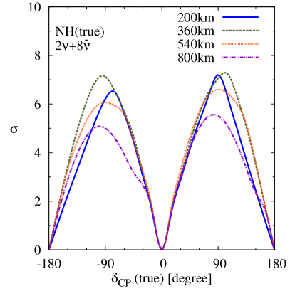
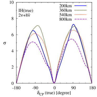
Figure 1: CP violation discovery potential (in $\sigma$) as a function of $\delta_{\mathrm{CP}}$(true). The left(right) panel assumes NH(IH) to be the true hierarchy. Baselines corresponding to 200 km, 360 km, 540 km and 800 km have been considered. The choice of run-plan is $2\nu+8{\bar{\nu}}$ years of running.

Fig. 1 shows that our results for CP violation are in agreement with those in Baussan et al. (2013). From the left panel of Fig. 1, it can be seen that for the 200 km baseline, which is the smallest amongst the four choices considered, a 3$\sigma~{}$C.L. evidence of CP violation is possible for 60% of $\delta_{\mathrm{CP}}$(true), while a 32% coverage is possible at 5$\sigma~{}$C.L. For the 540 km baseline, which shows the best sensitivities among the four choices considered, discovery of CP violation at the 3$\sigma~{}$C.L. is expected to be possible for 70% of $\delta_{\mathrm{CP}}$(true), while a 5$\sigma~{}$significance is expected for 45% of $\delta_{\mathrm{CP}}$(true). Thus, we are led to the conclusion that the 540 km choice is better-suited for the discovery of CP-violation with this set-up than any other choice of baseline. However, the CP violation discovery reach of the 360 km and 200 km baselines are only marginally lower. In particular, we note that if we have to change from the 540 km baseline to 200 km baseline, the CP coverage for CP violation discovery goes down only by $\sim$13% (10%) at the 5$\sigma~{}$(3$\sigma~{}$) C.L.

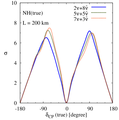
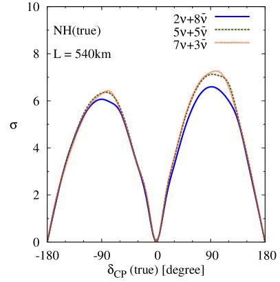
Figure 2: Statistical significance ($\sigma$) for CP violation discovery potential as a function of $\delta_{\mathrm{CP}}$(true). NH has been assumed to be the true hierarchy. The left(right) panel corresponds to the choice of 200 km (540 km) as the baseline. Results for different run-plans corresponding to $2\nu+8{\bar{\nu}}$, $5\nu+5{\bar{\nu}}$ and $7\nu+3{\bar{\nu}}$ years of running have been shown.

In Baussan et al. (2013), the nominal choice for the neutrino vs. anti-neutrino run-plan for the ESS$\nu$SB was taken as $2\nu+8{\bar{\nu}}$. The motivation behind this choice was to have similar number of events for both $\nu$ and ${\bar{\nu}}$ running. However, in order to explore this further, we calculate the sensitivity to CP violation for different run-plans. We have taken three cases: $2\nu+8{\bar{\nu}}$, $5\nu+5{\bar{\nu}}$, and $7\nu+3{\bar{\nu}}$. The left (right) panel in Fig. 2 shows the projected CP discovery potential for the 200 km (540 km) baseline option, for different run-plans. From these plots, it can be seen that at lower C.L., all the three run-plans have similar sensitivity. However, at 5$\sigma~{}$C.L., the larger coverage in $\delta_{\mathrm{CP}}$ comes with $7\nu+3{\bar{\nu}}$ running. While this holds true for both 200 km and 540 km, the effect is marginally more pronounced for the 200 km baseline option.

4.2 Precision on atmospheric parameters

We now focus on the achievable precision on atmospheric parameters with the proposed set-up. The precision is mainly governed by the $P(\nu_{\mu}\rightarrow\nu_{\mu})$ channel (see Eq. (1)). Because of huge statistics in this channel, we expect this set-up to pin down the atmospheric parameters to ultra-high precision. Indeed, this is the case as can be seen from Table 2. Table 2 shows the relative 1$\sigma~{}$precision on $\Delta m^{2}_{\mu\mu}$ and $\sin^{2}{\theta_{23}}$ considering three different values of true $\sin^{2}{\theta_{23}}$. Here, we have taken the baseline to be 200 km and the run-plan to be $7\nu+3{\bar{\nu}}$.

$\sin^{2}{\theta_{23}}$(true)	0.4	0.5	0.6
$\delta(\Delta m^{2}_{\mu\mu})$	0.24%	0.2%	0.22%
$\delta(\sin^{2}{\theta_{23}})$	1.12%	3.0%	0.8%

Table 2: Relative 1$\sigma~{}$precision (1 dof) on $\Delta m^{2}_{\mu\mu}$ and $\sin^{2}{\theta_{23}}$ considering three different values of true $\sin^{2}{\theta_{23}}$. Here, for all the cases, we consider the true value of $\Delta m^{2}_{\mu\mu}$ to be $2.4\times 10^{-3}\mathrm{eV^{2}}$. We consider NH as the true hierarchy. We have considered the 200 km as the baseline and $7\nu+3{\bar{\nu}}$ as the run-plan for generating these numbers.

It can be seen that around 0.2% precision on the atmospheric mass splitting is achievable which is a factor of $\sim 5$ better than what can be achieved with combined data from T2K and NO$\nu$A Agarwalla et al. (2013c). While the precision on $\Delta m^{2}_{\mu\mu}$ is weakly-dependent on the true value of $\sin^{2}{\theta_{23}}$, the precision in $\sin^{2}{\theta_{23}}$ shows a large dependence on its central value. We see that for $\sin^{2}{\theta_{23}}=0.5$, the precision is 3.0%, while for $\sin^{2}{\theta_{23}}=0.6$, its 0.8%. The precision in $\sin^{2}{\theta_{23}}$ is worst for the maximal mixing due to the fact that a large Jacobian is associated with transformation of the variable from $\sin^{2}2{\theta_{23}}$ to $\sin^{2}{\theta_{23}}$ around the maximal mixing Minakata et al. (2004).

4.3 Deviation from maximality

As discussed in the Introduction, currently different data sets have a conflict regarding the best-fit value of $\theta_{23}$ and its deviation from maximal mixing. While global analysis of all data hint at best-fit $\theta_{23}$ being non-maximal, these inferences depend on the assumed true mass hierarchy and are also not statistically very significant. Therefore, these results would need further corroboration in the next-generation experiments. If the deviation of $\theta_{23}$ from maximal mixing is indeed small, it may be difficult for the present generation experiment to establish a deviation from maximality. It has been checked that the combined results from T2K and NO$\nu$A will be able to distinguish a non-maximal value of $\theta_{23}$ from the maximal value $\pi/4$ at $3\sigma$ C.L. if $\sin^{2}\theta_{23}$(true)$\lesssim 0.45$ and $\gtrsim 0.57$. In such a situation, it will be interesting to know how well the ESS$\nu$SB set-up can establish a non-maximal $\sin^{2}{\theta_{23}}$. In Fig. 3, we show the sensitivity of various baselines towards establishing a non-maximal $\sin^{2}{\theta_{23}}$. These plots show the $\Delta\chi^{2}$ as a function of the true $\sin^{2}{\theta_{23}}$, where $\Delta\chi^{2}$ is as defined in section 3.

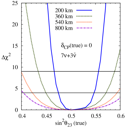
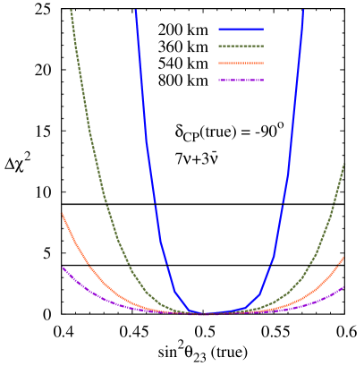
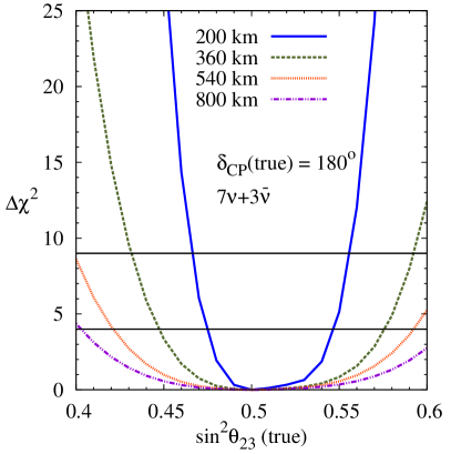
Figure 3: $\Delta\chi^{2}_{\textrm{min}}$ for a non-maximal ${\theta_{23}}$ discovery vs. $\sin^{2}{\theta_{23}}$(true) for the ESS$\nu$SB set-up. NH has been assumed to be the true hierarchy and the choice of run-plan has been taken to be $7\nu+3{\bar{\nu}}$ years of running. Results corresponding to various choices: 200 km, 360 km, 540 km and 800 km for the baseline have been shown. The top-left/top-right/bottom-left/bottom-right panel corresponds to $0$/$90^{\circ}$/$-90^{\circ}$/$180^{\circ}$ assumed as $\delta_{\mathrm{CP}}$(true). The horizontal black lines show 2$\sigma~{}$and 3$\sigma~{}$confidence level values.

The results are shown for the prospective baselines of 200 km, 360 km, 540 km and 800 km. The top left (right) panel corresponds to the choice of $\delta_{\mathrm{CP}}$ (true) of $0$ ($90^{\circ}$). The bottom left (right) panel corresponds to the choice of true $\delta_{\mathrm{CP}}$ of $-90^{\circ}$ ($180^{\circ}$). The true hierarchy for all these plots is assumed to be NH and the run-plan is taken to be $7\nu+3{\bar{\nu}}$. Here, we have marginalized the $\Delta\chi^{2}$ over the hierarchy. It can be seen from Fig. 3 that the best sensitivity occurs for the 200 km baseline. For true $\delta_{\mathrm{CP}}=0$, a 3$\sigma~{}$determination of non-maximal $\sin^{2}2{\theta_{23}}$ can be made if $\sin^{2}{\theta_{23}}\lesssim 0.47$ or if $\sin^{2}{\theta_{23}}\gtrsim 0.56$. A 5$\sigma~{}$determination is possible if $\sin^{2}{\theta_{23}}\lesssim 0.45$ or if $\sin^{2}{\theta_{23}}\gtrsim 0.57$. We checked that the contribution to the sensitivity from the appearance channels is small compared to that from the disappearance channels. This is reflected in the fact that there is a small dependence of $\Delta\chi^{2}$ on the assumed true value of $\delta_{\mathrm{CP}}$. An interesting observation is that the $\Delta\chi^{2}$ curve is not symmetric around the $\sin^{2}{\theta_{23}}=0.5$ line. It seems that, as far as observing a deviation from maximality is concerned, the lower octant is more favored than the higher octant. The reason behind this feature is the following. The sensitivity here, is mostly governed by the disappearance data in which the measured quantity is $\sin^{2}2\theta_{\mu\mu}$. Since $\sin^{2}{\theta_{23}}=\sin^{2}\theta_{\mu\mu}/\cos^{2}{\theta_{13}}$ Nunokawa et al. (2005); de Gouvea et al. (2005); Raut (2013), the ${\theta_{13}}$ correction shifts the $\theta_{23}$ values towards $45^{\circ}$ in the lower octant and away from $45^{\circ}$ in the higher octant. This results in the shifting of the curve towards the right in $\sin^{2}\theta_{23}$ and is reflected as the asymmetric nature of the curve. We have checked that for the (now) academic case of $\theta_{13}$(true)$=0$, the $\Delta\chi^{2}$ curve is symmetric around $45^{\circ}$.

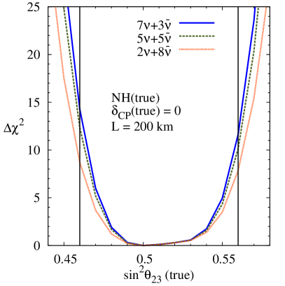
Figure 4: $\Delta\chi^{2}_{\textrm{min}}$ for a non-maximal ${\theta_{23}}$ discovery vs. $\sin^{2}{\theta_{23}}$ (true) for the ESS$\nu$SB set-up. NH has been assumed to be the true hierarchy and $\delta_{\mathrm{CP}}$(true) has been assumed to be 0. The choice of baseline has been taken to be 200 km. Results corresponding to various choices: $2\nu+8{\bar{\nu}}$, $5\nu+5{\bar{\nu}}$ and $7\nu+3{\bar{\nu}}$ years of running for the run-plan have been shown. The purpose of having vertical lines at $\sin^{2}{\theta_{23}}~{}\textrm{true}=0.46$ and 0.56 is to show the effect of run-plan on sensitivity (see Table 3 for discussion on this).

To find an optimal run-plan in the case of deviation from maximality, we generated the results for 200 km baseline for ESS$\nu$SB set-up, assuming NH and $\delta_{\mathrm{CP}}=0$. Three run-plans were assumed as before: $2\nu+8{\bar{\nu}}$, $5\nu+5{\bar{\nu}}$ and $7\nu+3{\bar{\nu}}$. It can be seen from Fig. 4 that the best results are observed for $7\nu+3{\bar{\nu}}$. Thus, this run-plan seems to be optimally suited for measurement of deviation from maximality as well. Note that apparently it seems from Fig. 4 that the sensitivity in the case of different run-plans are roughly the same despite there being huge change of statistics in terms of neutrino and anti-neutrino data. However, a closer look will reveal that the $\Delta\chi^{2}$ indeed changes as expected with the increase in the total statistics collected by the experiment and in fact it is the very sharp rise of the curves which hides the difference. To illustrate this further, we show in Table 3 the $\Delta\chi^{2}$ values corresponding to different run-plans at different true $\sin^{2}{\theta_{23}}$ values and for two choices of $\sin^{2}\theta_{23}$(true).

$\sin^{2}{\theta_{23}}$ (true)	$2\nu+8{\bar{\nu}}$	$5\nu+5{\bar{\nu}}$	$7\nu+3{\bar{\nu}}$
0.46	8.7	12.3	14.2
0.56	7.8	10.1	11.6

Table 3: $\Delta\chi^{2}_{\textrm{min}}$ for $\sin^{2}{\theta_{23}}$ (true) = 0.46 and 0.56. Here, the sensitivity of the ESS$\nu$SB set-up to the deviation from a maximal ${\theta_{23}}$ has been considered. NH has been assumed to be the true hierarchy and $\delta_{\mathrm{CP}}$(true) has been assumed to be 0. The choice of baseline has been taken to be 200 km. Results corresponding to various choices: $2\nu+8{\bar{\nu}}$, $5\nu+5{\bar{\nu}}$ and $7\nu+3{\bar{\nu}}$ years of running for the run-plan have been shown in different columns.

4.4 Octant resolution

In this section, we explore the octant resolving capability of the ESS$\nu$SB set-up. As discussed in the previous section, we generate true event rates at certain $\sin^{2}\theta_{23}$(true) and fit this by marginalizing over the entire $\sin^{2}\theta_{23}$ range in the wrong octant. The $\Delta\chi^{2}$ is also marginalized over $|\Delta m^{2}_{31}|$, $\sin^{2}\theta_{13}$, $\delta_{\mathrm{CP}}$ and the neutrino mass hierarchy. Fig. 5 shows the $\Delta\chi^{2}$ obtained as a function of $\sin^{2}{\theta_{23}}$(true) assuming NH to the true hierarchy. The corresponding results for the IH(true) case is shown in Fig. 6. We show the results for 200 km, 360 km, 540 km, and 800 km baselines in the first, second, third, and fourth rows respectively. The first column corresponds to the $2\nu+8{\bar{\nu}}$ run-plan. The second column corresponds to the $5\nu+5{\bar{\nu}}$ run-plan while the third column corresponds to the $7\nu+3{\bar{\nu}}$ run-plan. The band in each of these plots correspond to variation of $\delta_{\mathrm{CP}}$(true) in the range $[-180^{\circ},180^{\circ}]$. Thus, for any $\sin^{2}\theta_{23}$(true), the top-most and the bottom-most $\Delta\chi^{2}$ values lying in the band shows the maximum and minimum $\Delta\chi^{2}$ possible depending on the true value of $\delta_{\mathrm{CP}}$.

From the plots in Fig. 5 and Fig. 6, it can be seen that the best choice for $\theta_{23}$ octant resolution seems to be the 200 km baseline. Since amongst the various choices, the 200 km baseline is the closest to the source, it has the largest statistics for both $\nu$ and ${\bar{\nu}}$ samples. This is the main reason why the 200 km option returns the best octant resolution prospects. We have explicitly checked that if the statistics of the the other baseline options were scaled to match the one we get for the 200 km baseline option, they would give $\theta_{23}$ octant sensitivity close to that obtained for the 200 km option. We can also see from these figures that the best sensitivity is expected for the run-plan of $7\nu+3{\bar{\nu}}$. Note also that the $5\nu+5{\bar{\nu}}$ run-plan is just marginally worse than the $7\nu+3{\bar{\nu}}$ plan. However, these two run-plans are better than $2\nu+8{\bar{\nu}}$ run-plan. This again comes because of the fact that this option allows for larger statistics while maintaining a balance between the $\nu$ and ${\bar{\nu}}$ data, which is required to cancel degeneracies for maximum octant resolution capability as was shown in Agarwalla et al. (2013b). The impact of the run plans are again seen to be larger for the larger baselines. We can also see that the impact of $\delta_{\mathrm{CP}}$(true) is larger for larger baselines. The $\delta_{\mathrm{CP}}$ band is narrowest for the 200 km baseline option, implying that this baseline choice suffers least uncertainty from unknown $\delta_{\mathrm{CP}}$(true) for octant studies.

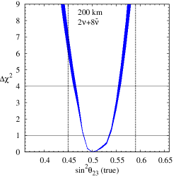
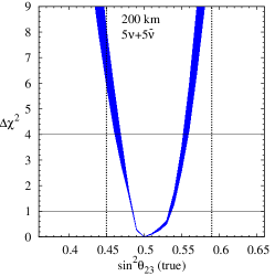
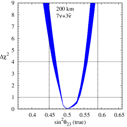
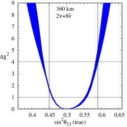
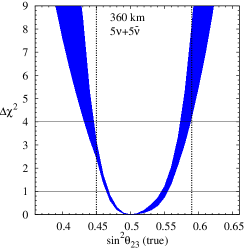
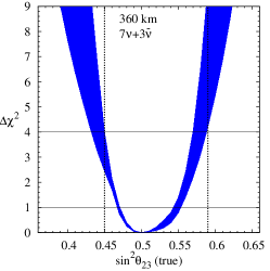
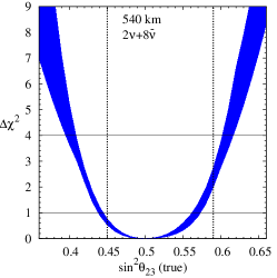
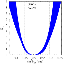
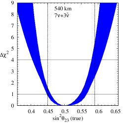
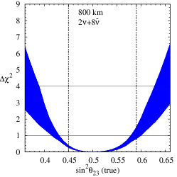
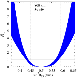
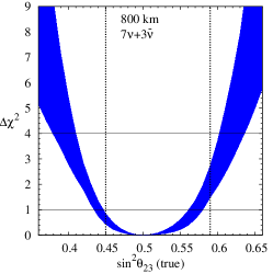
Figure 5: Octant resolution potential as a function of $\sin^{2}{\theta_{23}}$(true) for the ESS$\nu$SB set-up. NH has been assumed as the true hierarchy. The variation in the assumed value of $\delta_{\mathrm{CP}}$(true) leads to the formation of the band. Results corresponding to various run-plans and the assumed baseline for ESS$\nu$SB set-up have been shown. The rows correspond to 200 km, 360 km, 540 km, and 800 km from top to bottom and the columns correspond to $2\nu+8{\bar{\nu}}$, $5\nu+5{\bar{\nu}}$ and $7\nu+3{\bar{\nu}}$ years of running, from left to right. The horizontal black lines show 1$\sigma~{}$and 2$\sigma~{}$confidence level values.

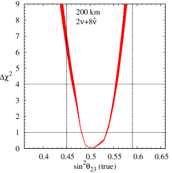
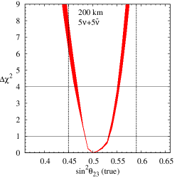
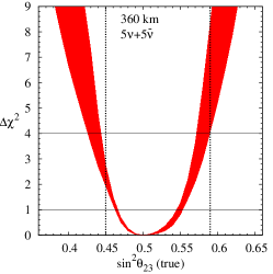
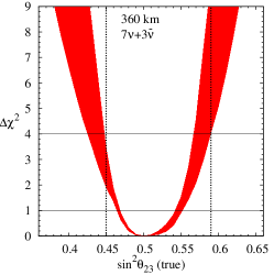
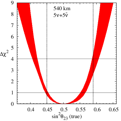
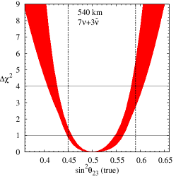
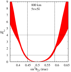
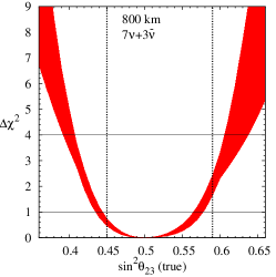
Figure 6: Octant resolution potential as a function of $\sin^{2}{\theta_{23}}$(true) for the ESS$\nu$SB set-up. IH has been assumed as the true hierarchy. The variation in the assumed value of $\delta_{\mathrm{CP}}$(true) leads to the formation of the band. Results corresponding to various run-plans and the assumed baseline for ESS$\nu$SB set-up have been shown. The rows correspond to 200 km, 360 km, 540 km, and 800 km from top to bottom and the columns correspond to $2\nu+8{\bar{\nu}}$, $5\nu+5{\bar{\nu}}$ and $7\nu+3{\bar{\nu}}$ years of running, from left to right. The horizontal black lines show 1$\sigma~{}$and 2$\sigma~{}$confidence level values.

Assuming NH(true) and with the 200 km baseline and $7\nu+3{\bar{\nu}}$ run-plan option, one can expect to resolve the correct octant of $\theta_{23}$ at the $3\sigma$ level for $\sin^{2}\theta_{23}$(true)$\lesssim 0.43$ and $\gtrsim 0.59$ irrespective of $\delta_{\mathrm{CP}}$(true). Correct octant can be identified with this option at 5$\sigma~{}$confidence level for $\sin^{2}\theta_{23}$(true)$\lesssim 0.37$ and $\gtrsim 0.63$ for all values of $\delta_{\mathrm{CP}}$(true). For IH(true) the corresponding values for $3\sigma$ ($5\sigma$) sensitivity are $\sin^{2}\theta_{23}$(true)$\lesssim 0.43(0.37)$ and $\gtrsim 0.59(0.62)$. These numbers and a comparison of Fig. 5 and 6 reveals that the octant sensitivity of the ESS$\nu$SB set-up does not depend much on the assumed true mass hierarchy. The octant sensitivity for both true hierarchies and all run-plan options is seen to deteriorate rapidly with the increase in the baseline. For the 540 km baseline option, we find that even for $\sin^{2}\theta_{23}$(true)$>0.35$ and $<0.63$, we do not get a $3\sigma$ resolution of the octant for 100% values of $\delta_{\mathrm{CP}}$(true).

To show the impact of $\delta_{\mathrm{CP}}$(true) on the determination of the octant of $\theta_{23}$ at ESS$\nu$SB, we show in Fig. 7 the $3\sigma$ contours in the $\sin^{2}\theta_{23}$(true)-$\delta_{\mathrm{CP}}$(true) plane for different baselines. We assume the $7\nu+3{\bar{\nu}}$ run-plan for this figure. The left hand panel shows the contours for NH(true) while the right hand panel is for IH(true). The different lines show the contours for the different baselines. Comparison of the different lines reveals that the 200 km baseline is better-suited for the resolution of octant. Not only does it gives the best octant determination potential, it also shows least $\delta_{\mathrm{CP}}-\sin^{2}{\theta_{23}}$ correlation. For other baselines, the contours fluctuate more depending on $\delta_{\mathrm{CP}}$(true) as for these baselines, the ESS fluxes peak close to the second oscillation maximum, where a larger sensitivity to $\delta_{\mathrm{CP}}$ exists. Hence, we see larger dependence of the sensitivity on the assumed true value of $\delta_{\mathrm{CP}}$. In particular, the performance is seen to be worst for $\delta_{\mathrm{CP}}$(true)$\simeq-90^{\circ}$ and best for $90^{\circ}$.

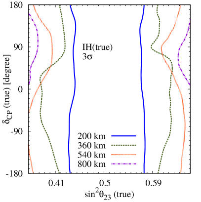
Figure 7: 3$\sigma~{}$C.L. contours in the $\sin^{2}{\theta_{23}}$(true)-$\delta_{\mathrm{CP}}$(true) plane for the octant-resolution sensitivity of the ESS$\nu$SB set-up. The left(right) panel corresponds to NH(IH) assumed as the true hierarchy. Results for various possible choices of baseline have been shown. The run-plan considered here is $7\nu+3{\bar{\nu}}$ years of running.

5 Summary and Conclusions

The ESS proposal is envisaged as a major European facility for neutron source, to be used for both research as well as the industry. A possible promising extension of this project could be to use it simultaneously to produce a high intensity neutrino superbeam to be used for oscillation physics. Since the energy of the beam is comparatively lower, it has been proposed to do this oscillation experiment at the second oscillation maximum, for best sensitivity to CP violation discovery. In this work we have made a comparative study of all oscillation physics searches with ESS$\nu$SB, allowing for all possible source-detector distances and with different run-plan options for running the experiment in the neutrino and anti-neutrino modes.

In particular, we have evaluated the sensitivities of the ESS$\nu$SB proposal towards the discovery of CP violation in the lepton sector, achievable precision on atmospheric parameters, deviation of $\sin^{2}{\theta_{23}}$ from 0.5, and finally the octant in which it lies. We have considered the prospective baselines - 200 km, 360 km, 540 km, and 800 km for the resolution of the above mentioned unknowns. We also tested different run-plans i.e. varying combination of $\nu$ and ${\bar{\nu}}$ data with a total of 10 years of running. We considered $2\nu+8{\bar{\nu}}$, $5\nu+5{\bar{\nu}}$ and $7\nu+3{\bar{\nu}}$. In the case of CP violation, we find that the best sensitivity comes for 540 km baseline where 70% coverage is possible in true $\delta_{\mathrm{CP}}$ at 3$\sigma~{}$while a 45% coverage is possible at 5$\sigma~{}$. For the 200 km baseline, we find that 60% coverage is possible at 3$\sigma~{}$and 32% coverage is possible at 5$\sigma~{}$. We further find that all the three run-plans give the same coverage at 2$\sigma~{}$C.L. but, at 5$\sigma~{}$C.L., a better coverage is possible with the $7\nu+3{\bar{\nu}}$ run-plan. For determination of deviation of $\theta_{23}$ from maximality, the best sensitivity is expected for the 200 km baseline with the $7\nu+3{\bar{\nu}}$ run-plan, as this combination provides the largest statistics. For true $\delta_{\mathrm{CP}}=0$, a 3$\sigma~{}$determination of non-maximal $\sin^{2}2{\theta_{23}}$ can be made if true value of $\sin^{2}{\theta_{23}}\lesssim 0.47$ or $\gtrsim 0.56$. A 5$\sigma~{}$determination is possible if the true value of $\sin^{2}{\theta_{23}}\lesssim 0.45$ or $\gtrsim 0.57$. In the case of octant also, we find that the 200 km baseline and $7\nu+3{\bar{\nu}}$ run-plan provides the best sensitivity. We find that, assuming NH to be the true hierarchy, a 3$\sigma~{}$resolution of octant is possible if $\sin^{2}\theta_{23}$(true) $\lesssim 0.43$ and $\gtrsim 0.59$ for all values of $\delta_{\mathrm{CP}}$(true). A $5\sigma$ determination could be possible if $\sin^{2}\theta_{23}$(true) $\lesssim 0.37$ and $\gtrsim 0.63$.

Finally, we end this paper with a comparison of the deviation from maximality and octant of $\theta_{23}$ discovery reach of the ESS$\nu$SB set-up with the other next-generation proposed long baseline superbeam experiments. We show in Fig. 8 this comparison for the ESS$\nu$SB set-up with the 200 km baseline option and $7\nu+3{\bar{\nu}}$ run-plan (green short dashed lines), LBNE with 10 kt liquid argon detector (orange dotted lines), and LBNO with 10 kt liquid argon detector (purple dot-dashed lines). For LBNE and LBNO, we have used the experimental specifications as given in Agarwalla et al. (2014). In generating the plots for these three future facilities, we have added the projected data from T2K ($2.5\nu+2.5{\bar{\nu}}$) and NO$\nu$A ($3\nu+3{\bar{\nu}}$). The details of these experiments are the same as considered in Agarwalla et al. (2012). The left hand panel of this figure shows the $\Delta\chi^{2}$ as a function of $\sin^{2}{\theta_{23}}$(true) for deviation of $\theta_{23}$ from its maximal value for $\delta_{\mathrm{CP}}$(true)$=0$. The ESS$\nu$SB set-up is seen to perform better than the other two superbeam options, mainly due to larger statistics. With larger detectors, both LBNE and LBNO will start to be competitive. The right hand panel shows $5\sigma$ contours for the octant of $\theta_{23}$ discovery reach in the $\delta_{\mathrm{CP}}$(true)-$\sin^{2}{\theta_{23}}$(true) plane. The three experiments are very comparable, with the best reach coming for the ESS$\nu$SB set-up with the 200 km baseline option and $7\nu+3{\bar{\nu}}$ run-plan.

To conclude, among all four choices of the baselines, the best results for sensitivity to deviation from maximality and resolution of octant is expected for the 200 km baseline option. On the other hand, chances for discovery of CP violation are best for the 540 km baseline, which sits on the second oscillation maximum and hence gives the maximum coverage in true $\delta_{\mathrm{CP}}$. However, the CP violation discovery prospects for the 200 km baseline is only slightly worse. We have also seen that for all oscillation physics results, the $7\nu+3{\bar{\nu}}$ run-plan provides the best sensitivity amongst the three run-plan choices considered. While we appreciate the merit of putting the detector at the second oscillation peak, this paper shows the advantage of another baseline option, in particular, 200 km.

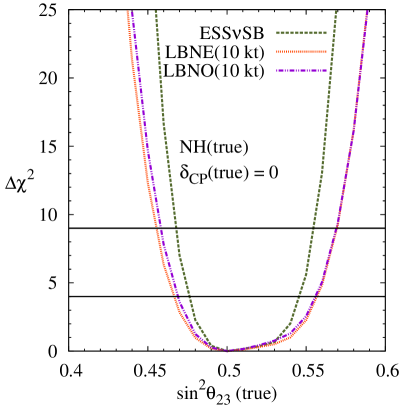
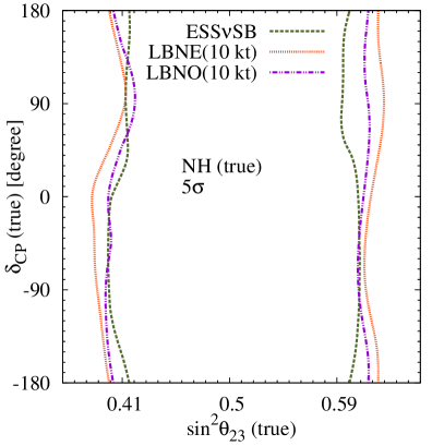
Figure 8: A comparison of the future facilities LBNE and LBNO with the ESS$\nu$SB set-up. Left panel: non-maximal ${\theta_{23}}$ discovery potential. Right panel: octant resolution potential. For ESS$\nu$SB, a 200 km long baseline and a $7\nu+3{\bar{\nu}}$ running is considered. For both LBNE and LBNO, a 10 kt LArTPC detector and a $5\nu+5{\bar{\nu}}$ running is considered. The horizontal black lines show 2$\sigma~{}$and 3$\sigma~{}$C.L.