Resolving $\theta_{23}$ Degeneracy by
Accelerator and Reactor Neutrino Oscillation Experiments

Abstract

If the lepton mixing angle $\theta_{23}$ is not maximal, there arises a problem of ambiguity in determining $\theta_{23}$ due to the existence of two degenerate solutions, one in the first and the other in the second octant. We discuss an experimental strategy for resolving the $\theta_{23}$ octant degeneracy by combining reactor measurement of $\theta_{13}$ with accelerator $\nu_{\mu}$ disappearance and $\nu_{e}$ appearance experiments. The robustness of the $\theta_{23}$ degeneracy and the difficulty in lifting it only by accelerator experiments with conventional $\nu_{\mu}$ (and $\bar{\nu}_{\mu}$) beam are demonstrated by analytical and numerical treatments. Our method offers a way to overcome the difficulty and can resolve the degeneracy between solutions $\sin^{2}\theta_{23}=0.4$ and $\sin^{2}\theta_{23}=0.6$ if $\sin^{2}2\theta_{13}\raise 1.29167pt\hbox{$\;>$\kern-7.5pt\raise-4.73611pt\hbox{$\sim\;$}}0.05$ at 95% CL by assuming the T2K phase II experiment and a reactor measurement with an exposure of 10 GW$\cdot$kt$\cdot$yr. The dependence of the resolving power of the octant degeneracy on the systematic errors of reactor experiments is also examined.

I introduction

The atmospheric neutrino observation by Super-Kamiokande (SK), which discovered neutrino oscillation, established that the mixing angle $\theta_{23}$ is large, which may be even close to the maximum SKatm . Then, it became clear that the solar mixing angle $\theta_{12}$ is also large, though not maximal, as indicated by accumulation of the solar and the reactor data solar ; KamLAND . Curiously enough, the third angle $\theta_{13}$ is known to be small CHOOZ ; K2K_app . Comprehending the structure of lepton mixing described by the Maki-Nakagawa-Sakata (MNS) matrix MNS which is composed of a nearly maximal, a large, and a small angle should reveal the key to understand the underlying physics of lepton flavor mixing.

Toward the explanation of the coexistence of nearly maximal and small mixing angles some symmetries symmetry which are motivated by more phenomenological $\mu\leftrightarrow\tau$ exchange symmetries mu-tau are discussed. Interestingly, most of them share an attractive feature that $\theta_{23}=\pi/4$ and $\theta_{13}=0$ in the symmetry limit, suggesting a possible common origin of the two small quantities in the lepton flavor mixing, $\theta_{13}$ and $D_{23}\equiv\frac{1}{2}-\sin^{2}\theta_{23}$, the parameter which measures deviation from the maximal mixing. The quark-lepton complementarity QLC , if extends to the 2-3 sector, might be relevant for maximal or nearly maximal $\theta_{23}$. If these small quantities take non-vanishing values it should give us a further hint for deciding if the symmetries are the right explanation for the two small quantities, and if so, for identifying the correct symmetry.

In this paper, we describe an experimental strategy for determining $\theta_{23}$ following MSYIS , where it was proposed that the $\theta_{23}$ octant degeneracy can be lifted by combining reactor measurement of $\theta_{13}$ with accelerator appearance and disappearance measurement of certain combinations of $\theta_{23}$ and $\theta_{13}$. See Ref. octant for an earlier suggestion of this possibility. We thoroughly examine this method by taking a concrete (and probably the best thinkable) setting for accelerator experiments, phase II of the T2K experiment JPARC , with Hyper-Kamiokande as a detector nakamura and a 4 MW neutrino beam from the J-PARC facility. For knowledges of reactor measurement, we are benefited by the outcome of the world-wide effort reactor_white . We carry out a detailed quantitative analysis to obtain the region of $\theta_{13}$ and $\theta_{23}$ in which the $\theta_{23}$ octant degeneracy can be resolved by our method. For a related analysis, see shaevitz .

The $\theta_{23}$ octant degeneracy is a part of a larger structure called the parameter degeneracy. It may be understood as the intrinsic degeneracy Burguet-C duplicated by the unknown sign of $\Delta m^{2}_{31}$ MNjhep01 and $\theta_{23}$ octant ambiguity octant , which lead to the total eight-fold degeneracy BMW1 . (See MNP2 for exposition of analytic structure of the degeneracies.) Then, one has to address a problem; Is it possible to resolve only the $\theta_{23}$ degeneracy, leaving the other two types of degeneracies untouched? We will answer in the positive this question in the context of conventional $\nu_{\mu}$ beam experiments. In short, in modest baseline distances for which perturbative treatment of the matter effect is valid, the $\theta_{23}$ degeneracy is decoupled from the other degeneracies and can be resolved independently in the presence of them.

The current bounds on these small quantities in the lepton flavor mixing are rather mild,

$$-0.14\leq D_{23}\equiv\frac{1}{2}-\sin^{2}\theta_{23}\leq 0.14,$$ (1)

at 90% CL SKatm , which is nothing but a translation of the bound $\sin^{2}2\theta_{23}\geq 0.92$. At present, there is neither indication of deviation from the maximal $\theta_{23}$, nor preference of the particular octant (apart from very slight preference of the 2nd octant) in the analysis by the SK group with their current data set kajita . On the other hand, the bound on $\theta_{13}$ is much stronger if one uses the same variable,

$$\sin^{2}\theta_{13}\leq 0.022~{}(0.047)$$ (2)

at 90% (3$\sigma$) CL for 1 degree of freedom, as obtained by the global analysis global with use of all the data including the Chooz, the atmospheric, and the K2K K2K one. As discussed in MSS04 (see also munich ), one of the major difficulties for accurate measurement of $\theta_{23}$ with accelerator neutrinos is the $\theta_{23}$ degeneracy. Hence, we expect that our method will help to improve the situation.

In Sec. II, we explain how the $\theta_{23}$ octant degeneracy can be resolved by our method. In Sec. III, we discuss how robust is the $\theta_{23}$ octant degeneracy by indicating the difficulties in resolving it only by accelerator measurement. In Sec. IV, we fully explain the statistical procedure of our analysis. In Sec. V, we present the results of our analysis. In Sec. VI, we give concluding remarks. In Appendix A, we describe some details of how the referred numbers of events are computed in our paper.

II The method and what is new?

For completeness of the presentation, we start by reviewing the method for solving $\theta_{23}$ octant degeneracy described in MSYIS . At the end of this section, we will try to elucidate the difference between this work and the reference MSYIS . We invite the readers to look at Fig. 1, and first focus on the upper four panels, the case where the input value of $\theta_{23}$ is in the first octant. (The upper four and the lower four panels of Fig. 1 are for input values of $s^{2}_{23}=0.458$ and 0.542, respectively.) Fig. 1a describes the constraints imposed by each accelerator experiment, $\nu_{\mu}$ (and $\bar{\nu}_{\mu}$) disappearance and $\nu_{e}$ (and $\bar{\nu}_{e}$) appearance measurement. Although these contours come from our full analysis whose details will be explained in Secs. IV and V, the main features of Fig. 1 can be understood by the vacuum oscillation approximation, and essentially it is all that we need.

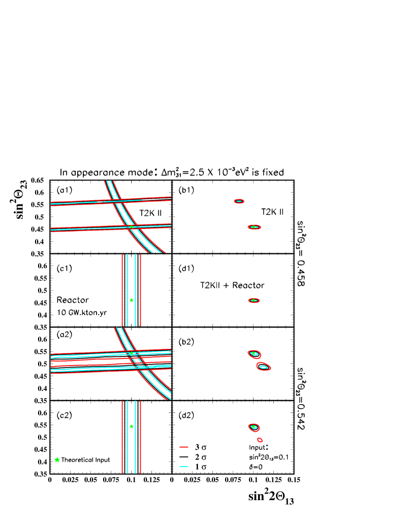
Figure 1: The upper (lower) four panels describe the process of how the $\theta_{23}$ octant degeneracy can be resolved for the case where the true value of $\sin^{2}\theta_{23}$ = 0.458 (0.542), corresponding to $\sin^{2}{2\theta_{23}}=0.993$. The other input mixing parameters are given as $\Delta m^{2}_{31}=2.5\times 10^{-3}$ eV², $\sin^{2}2\theta_{13}$ = 0.1 and $\delta=0$, $\Delta m^{2}_{21}=8.0\times 10^{-5}$ eV², $\sin^{2}\theta_{12}$ = 0.31 (the input values of $\sin^{2}2\theta_{13}$ and $\sin^{2}\theta_{23}$ are indicated by the symbol of star in the plot). (a) The regions enclosed by the solid and the dashed curves are allowed regions only by the results of appearance and disappearance accelerator measurement, respectively. (b) The regions that remain allowed when results of appearance and disappearance measurement are combined. (c) The regions allowed by reactor measurement. (d) The regions allowed after combining the results of appearance and disappearance accelerator experiments with the reactor measurement. The exposures for accelerator are assumed to be 2 (6) years of neutrino (anti-neutrino) running with 4 MW beam power with Hyper-Kamionande whose fiducial volume is 0.54 Mt, whereas for the reactor we assume an exposure of 10 GW$\cdot$kt$\cdot$yr. The case of optimistic systematic error is taken. (See Secs. IV and Appendix A for details.)

The $\nu_{\mu}$ disappearance and $\nu_{e}$ appearance probabilities in one $\Delta m^{2}$ dominance approximation one-mass , which may be justified by $\Delta m^{2}_{21}/\Delta m^{2}_{31}\simeq 1/30\ll 1$, are given by

$$P(\nu_{\mu}\rightarrow\nu_{\mu}) = 1-\sin^{2}2\theta_{23}\sin^{2}\Bigl{(}\frac{\Delta m^{2}_{31}L}{4E}\Bigr{)},$$ (3)

$$P(\nu_{\mu}\rightarrow\nu_{\rm e}) = s^{2}_{23}\sin^{2}{2\theta_{13}}\sin^{2}\left(\frac{\Delta m^{2}_{31}L}{4E}\right),$$ (4)

where $E$ denotes the neutrino energy and $L$ is the baseline distance. We use the standard notation of the MNS matrix including the symbol $s_{ij}$ for $\sin\theta_{ij}$ PDG . $\Delta m^{2}_{ji}$ is defined as $\Delta m^{2}_{ji}\equiv m^{2}_{j}-m^{2}_{i}$ by using the neutrino masses $m_{i}$ ($i=$ 1-3). In this approximation $P(\nu_{\alpha}\rightarrow\nu_{\beta})=P(\bar{\nu}_{\alpha}\rightarrow\bar{\nu}_{\beta})$. Accelerator disappearance measurement is expected to determine both $\Delta m^{2}_{31}$ and $\sin^{2}{2\theta_{23}}$ with high accuracies. It is obvious that, if $\theta_{23}\neq\pi/4$, one has two-fold solutions of $\theta_{23}$ for a given value of $\sin^{2}{2\theta_{23}}$; $s^{2}_{23}=\frac{1}{2}\left[1\pm\sqrt{1-\sin^{2}{2\theta_{23}}}\right]$. This is a simple illustration of how $\theta_{23}$ octant degeneracy arises. The almost horizontal two lines in Fig. 1a are nothing but these two solutions of $s^{2}_{23}$ for a given value of $\sin^{2}{2\theta_{23}}=0.993$.

On the other hand, accelerator appearance measurement determines a particular combination of two angles, $s^{2}_{23}\sin^{2}{2\theta_{13}}$, as seen in (4) for a given value of $\Delta m^{2}_{31}$. The latter quantity is expected to be well determined by disappearance measurement. The curved strip in Fig. 1a, which takes the approximate form $s^{2}_{23}\sin^{2}{2\theta_{13}}=\text{constant}$, is the outcome of the $\nu_{e}$ and $\bar{\nu}_{e}$ appearance measurement. In Fig. 1b we combine the disappearance and appearance measurement and we end up with a pair of degenerate solutions of $\theta_{13}$ and $\theta_{23}$.

Now, we combine the information from reactor experiments. In a very good approximation what they measure is equal to the vacuum oscillation probability $P(\bar{\nu}_{e}\rightarrow\bar{\nu}_{e})$ which is given again in the one $\Delta m^{2}$ dominance approximation as

$$P(\bar{\nu}_{e}\rightarrow\bar{\nu}_{e})=1-\sin^{2}{2\theta_{13}}\sin^{2}\left(\frac{\Delta m^{2}_{31}L}{4E}\right).$$ (5)

Given the value of $\Delta m^{2}_{31}$ by disappearance measurement, the reactor experiments determine $\theta_{13}$ independent of other mixing parameters. This is illustrated in Fig. 1c. When we combine the accelerator disappearance and appearance experiments as well as reactor measurement, one of the two allowed solutions in Fig. 1b disappears as shown in Fig. 1d. Thus, the $\theta_{23}$ octant degeneracy can be lifted.

Though using the same method as proposed in MSYIS , our analysis goes beyond that given in the reference in a number of ways. We have taken into account errors in accelerator disappearance and appearance as well as background so that the event number distributions roughly reproduce those obtained by the experimental group JPARC-detail ; Hiraide . Our treatment of the reactor measurement of $\theta_{13}$ is elaborated to include uncorrelated and correlated errors in order to treat the so called phase II type high statistics measurement. By using the highest sensitivity reactor and accelerator experiments, we aim at revealing the ultimate sensitivity for resolution of the $\theta_{23}$ octant degeneracy achievable by this method. Differences between this paper and MSYIS exist not only in the method for the analysis but also in some features of the results. For the particular set of parameters used in Fig. 1, the resolving power of the $\theta_{23}$ degeneracy is greater for the case with true values of $\theta_{23}$ in the first octant than for the case in the second octant. It is in disagreement with the naive expectation in MSYIS based on the difference between $\theta_{23}$ of a true and a fake solutions. See Sec. V for more details.

III The $\theta_{23}$ octant degeneracy is hard to resolve by accelerator experiments

We illustrate how difficult is to resolve the octant degeneracy by accelerator experiments with conventional neutrino beam. Apparently, this fact has been recognized by people in the community, but to our knowledge, a coherent discussion of why it is so has never been given. Therefore, we try to fill the gap. As a byproduct, the argument illuminates the nature of the $\theta_{23}$ degeneracy and may indicate a unique feature of our approach. We note that, strictly speaking, our following discussion in this section is valid under circumstances that the matter effect can be treated perturbatively, and hence for baseline shorter than $L\simeq 1000$ km. (See below.)

III.1 The octant degeneracy is robust

Robustness of the degeneracy is obvious from Fig. 1a and Fig. 1b, but we want to elaborate the discussion to bring our understanding to a little deeper level. The reasons for the robustness are mainly twofold:

• The difference in energy spectra predicted by degenerate solutions in either the appearance or disappearance channels is too small to distinguish between the first- and the second-octant solutions.

• The matter effects in the disappearance channels are not strong enough to lift the octant degeneracy, unless one goes to very long baseline.

To explain the first point, we introduce the quantity $\Delta P_{12}(\nu_{\alpha}\rightarrow\nu_{\beta})$,

$$\Delta P_{12}(\nu_{\alpha}\rightarrow\nu_{\beta})\equiv P(\nu_{\alpha}\rightarrow\nu_{\beta};\theta_{23}^{\text{1st}},\theta_{13}^{\text{1st}})-P(\nu_{\alpha}\rightarrow\nu_{\beta};\theta_{23}^{\text{2nd}},\theta_{13}^{\text{2nd}}),$$ (6)

the difference between probabilities with parameters of two degenerate solutions, $\theta_{23}^{i}$ and $\theta_{13}^{i}$ (i=1st, 2nd), determined at a particular value of energy in this exercise. In Fig. 2, plotted are $\Delta P_{12}(\nu_{\mu}\rightarrow\nu_{e})$ (left upper panel), $\Delta P_{12}(\nu_{\mu}\rightarrow\nu_{\mu})$ (right upper panel), and their antineutrino counterparts in the lower two panels. As one can see in Fig. 2, $\Delta P_{12}$’s are less than $\sim 0.2$% in most of the energy region. In this exercise, the CP phase $\delta^{\text{i}}$ (i=1st, 2nd) is kept equal and we did not try to adjust it to make $\Delta P_{12}$ smaller. We have also examined three other values of delta, $\delta=\pi/2,\pi,3\pi/2$, in addition to the $\delta=0$ case in Fig. 2, and reached the same conclusion.

The smallness of $\Delta P_{12}(\nu_{\mu}\rightarrow\nu_{e})$ and $\Delta P_{12}(\nu_{\mu}\rightarrow\nu_{\mu})$ discourages the possibility of resolution of the $\theta_{23}$ octant degeneracy by using spectrum informations. This is in sharp contrast to the case of intrinsic degeneracy of $\theta_{13}$-$\delta$, for which the spectrum analysis is proved to be powerful in the presently discussed original T2K setting provided that $\theta_{13}$ is not too small T2KK .

Figure 2: Two examples of the $\theta_{23}$ degenerate solutions are shown to have almost the same energy spectrum in Kamioka with baseline of 295 km from J-PARC. In the upper (lower) panels, we show the difference of the probabilities of two degenerate solutions for neutrino (anti-neutrino) channels. The solid and the dashed lines are for normal ($\Delta m^{2}_{31}>0$) and the inverted ($\Delta m^{2}_{31}<0$) mass hierarchies, respectively.

III.2 Approximate analytic treatment of the $\theta_{23}$ octant degeneracy

We present an analytic framework to understand better the reasons for the robustness of the $\theta_{23}$ octant degeneracy. We restrict ourselves to baselines where the earth matter effect can be treated as perturbation in the appearance channel. For a consistent treatment we start from the expression of the disappearance probability $P(\nu_{\mu}\rightarrow\nu_{\mu})$ in the one $\Delta m^{2}$ dominant vacuum oscillation approximation but with leading order $s^{2}_{13}$ correction

$$1-P(\nu_{\mu}\rightarrow\nu_{\mu})=\left[\sin^{2}2\theta_{23}+4s^{2}_{13}s^{2}_{23}\left(2s^{2}_{23}-1\right)\right]\sin^{2}\left(\frac{\Delta m^{2}_{31}L}{4E}\right).$$ (7)

Then, a disappearance measurement determines $s^{2}_{23}$ to first order in $s^{2}_{13}$ as $(s^{2}_{23})^{(1)}=(s^{2}_{23})^{(0)}(1+s^{2}_{13})$ where $(s^{2}_{23})^{(0)}$ is the solution obtained by ignoring $s^{2}_{13}$. By reading off the coefficient of sine squared term in (7), one can determine $\sin^{2}{2\theta_{23}}$ and $s^{2}_{23}$ is given by $(s^{2}_{23})^{(0)}=\frac{1}{2}\left[1\pm\sqrt{1-\sin^{2}{2\theta_{23}}}\right]$ as noted before. We note that the linear dependence of $(s^{2}_{23})^{(1)}$ on $s^{2}_{13}$ is clearly seen in Fig. 1a.

For the appearance channel, we use the $\nu_{e}$ ($\bar{\nu}_{e}$) appearance probability with first-order matter effect AKS

$$P[\nu_{\mu}(\bar{\nu}_{\mu}) \rightarrow \nu_{\rm e}(\bar{\nu}_{e})]$$ (8)

$$= \sin^{2}{2\theta_{13}}s^{2}_{23}\left[\sin^{2}\left(\frac{\Delta m^{2}_{31}L}{4E}\right)-\frac{1}{2}s^{2}_{12}\left(\frac{\Delta m^{2}_{21}L}{2E}\right)\sin\left(\frac{\Delta m^{2}_{31}L}{2E}\right)\right.$$

$$\hskip 62.59605pt{}\pm\left.\left(\frac{4Ea(x)}{\Delta m^{2}_{31}}\right)\sin^{2}{\left(\frac{\Delta m^{2}_{31}L}{4E}\right)}\mp\frac{a(x)L}{2}\sin\left(\frac{\Delta m^{2}_{31}L}{2E}\right)\right]$$

$$+2J_{r}\left(\frac{\Delta m^{2}_{21}L}{2E}\right)\left[\cos{\delta}\sin\left(\frac{\Delta m^{2}_{31}L}{2E}\right)\mp 2\sin{\delta}\sin^{2}\left(\frac{\Delta m^{2}_{31}L}{4E}\right)\right].$$

In (8), $a(x)=\sqrt{2}G_{F}N_{e}(x)$ MSW where $G_{F}$ is the Fermi constant, $N_{e}(x)$ denotes the electron number density at the point $x$ in the earth, $J_{r}$ $(=c_{12}s_{12}c_{13}^{2}s_{13}c_{23}s_{23})$ denotes the reduced Jarlskog factor, and the upper and the lower sign $\pm$ refer to the neutrino and anti-neutrino channels, respectively.

We make an approximation of ignoring terms of order $(\Delta m^{2}_{21}/\Delta m^{2}_{31})J_{r}\cos{2\theta_{23}}$. Note that keeping only the leading order in this quantity is reasonable because $J_{r}<0.04$, $\Delta m^{2}_{21}/\Delta m^{2}_{31}\simeq 1/30$, and $\cos{2\theta_{23}}=\pm 0.2$ for $\sin^{2}{2\theta_{23}}=0.96$. Then, the two degenerate solutions obey an approximate relationship

$$\left(\sin^{2}{2\theta_{13}}s^{2}_{23}\right)^{1st}=\left(\sin^{2}{2\theta_{13}}s^{2}_{23}\right)^{2nd},$$ (9)

or, $s_{13}^{1st}s_{23}^{1st}=s_{13}^{2nd}s_{23}^{2nd}$ ignoring higher order terms in $s_{13}$. We can neglect the leading order correction in $s^{2}_{13}$ to $s^{2}_{23}$ in these relations because it gives $O(s^{4}_{13})$ terms.

III.3 Appearance channel; $\nu_{\mu}\rightarrow\nu_{e}$

With our machinery well oiled we can understand better the behavior of $\Delta P_{12}(\nu_{\mu}\rightarrow\nu_{e})$ and $\Delta P_{12}(\nu_{\mu}\rightarrow\nu_{\mu})$ given in Fig. 2, in particular their small values, $\sim 10^{-3}$. We also note that even if we switch off the matter effect, there is no visible change in $\Delta P_{12}(\nu_{\mu}\rightarrow\nu_{e})$ and $\Delta P_{12}(\bar{\nu}_{\mu}\rightarrow\bar{\nu}_{e})$ in Fig. 2. Now, these features can be understood in our analytic framework.

Noting that $J_{r}^{1st}-J_{r}^{2nd}=\cos{2\theta_{23}^{1st}}J_{r}^{1st}$ in leading order in $\cos{2\theta_{23}}$, the difference between probabilities with the first and the second octant solutions can be given by

$$\Delta P_{12}(\nu_{\mu}\rightarrow\nu_{e})$$ (10)

$$= 2J_{r}^{1st}\cos{2\theta_{23}^{1st}}\left(\frac{\Delta m^{2}_{21}L}{2E}\right)\left[\cos{\delta}\sin\left(\frac{\Delta m^{2}_{31}L}{2E}\right)\mp 2\sin{\delta}\sin^{2}\left(\frac{\Delta m^{2}_{31}L}{4E}\right)\right].$$

The size of $\Delta P_{12}$ is about $\simeq 10^{-3}$ for $\cos{2\theta_{23}}=0.2$, which is roughly consistent with the results given in Fig. 2. The remarkable feature of (10) is that the leading-order matter effect terms drops out completely, because they depend upon $\theta_{23}$ and $\theta_{13}$ only though the invariant combination (9). Therefore, we suspect that our statement about robustness of the $\theta_{23}$ octant degeneracy may apply not only to the T2K experiment but also to experiments with longer baseline, including the NO$\nu$A project NOVA .

III.4 Disappearance channel; $\nu_{\mu}\rightarrow\nu_{\mu}$

Does the disappearance channel $\nu_{\mu}\rightarrow\nu_{\mu}$ help? Using the approximate relationship (9) and the first order (in $s^{2}_{13}$) corrected formula for $s^{2}_{23}$ mentioned after (7), we obtain the expression of $\Delta P_{12}(\nu_{\mu}\rightarrow\nu_{\mu})$ to first order in matter effect as a sum of the vacuum and the matter effect contributions, $\Delta P_{12}(\nu_{\mu}\rightarrow\nu_{\mu})=\Delta P_{12}(\nu_{\mu}\rightarrow\nu_{\mu})_{\text{vac}}+\Delta P_{12}(\nu_{\mu}\rightarrow\nu_{\mu})_{\text{matter}}$. The vacuum term

$$\Delta P_{12}(\nu_{\mu} \rightarrow \nu_{\mu})_{\text{vac}}=$$ (11)

$$2\cos 2\theta_{23}^{\text{1st}}\left[-\left(s^{2}_{13}s^{2}_{23}\right)^{\text{1st}}+\sqrt{2}s_{23}^{\text{1st}}J_{r}^{\text{1st}}\cos\delta\right]\left(\frac{\Delta m^{2}_{21}L}{2E}\right)\sin\left(\frac{\Delta m^{2}_{31}L}{2E}\right)$$

is small, $\sim 10^{-3}$, because of the suppression by either one of $s^{2}_{13}$ or $J_{r}$, and $\Delta m^{2}_{21}/\Delta m^{2}_{31}$.

The matter term is given by AKS

$$\Delta P_{12}(\nu_{\mu} \rightarrow \nu_{\mu})_{\text{matter}}=2P(\nu_{\mu}\rightarrow\nu_{\mu})_{\text{matter}}=2(aL)\sin^{2}2\theta_{13}s_{23}^{2}D_{23}F(x),$$ (12)

where $D_{23}\equiv\frac{1}{2}-s^{2}_{23}$, $x\equiv\frac{\Delta m^{2}_{31}L}{2E}$ and the function $F$ is defined as $F(x)\equiv\frac{4}{x}\sin^{2}\left(\frac{x}{2}\right)-\sin x$. Since the term flips sign under the transformation $\theta_{23}\rightarrow\pi/2-\theta_{23}$, it may be used to discriminate if $\theta_{23}<\pi/4$ or $\theta_{23}>\pi/4$ choubey . Unfortunately, the size of (12) and hence its contribution to $\Delta P_{12}(\nu_{\mu}\rightarrow\nu_{\mu})$ is small,

$$(\Delta P_{12})_{\text{matter}}\simeq 5.2\times 10^{-3}F(x)\left(\frac{\sin^{2}2\theta_{13}}{0.1}\right)\left(\frac{D_{23}}{0.1}\right)\left(\frac{\rho}{2.8\mbox{ gcm}^{-3}}\right)\left(\frac{L}{1000\mbox{ km}}\right).$$ (13)

Note that $F$ is a monotonically increasing function of $x$ in $0<x\raise 1.29167pt\hbox{$\;<$\kern-7.5pt\raise-4.73611pt\hbox{$\sim\;$}}4$, and $F(\pi)=4/\pi=1.273$. Thus, the difference $(\Delta P_{12})_{\text{matter}}$ is of order $10^{-3}$ at $L=300$ km (less than 1% even at $L=1000$ km) with $\theta_{13}$ at around the Chooz limit CHOOZ .

It should be noticed that $\Delta P_{12}$ flips sign not only under $D_{23}\rightarrow-D_{23}$ but also under $\Delta m^{2}_{31}\rightarrow-\Delta m^{2}_{31}$. Therefore, measurement of the sign of $\Delta P_{12}$ determines the combined sign, $\Delta m^{2}_{31}\times D_{23}$. Hence, the use of this effect to resolve the $\theta_{23}$ degeneracy requires prior knowledge of the neutrino mass hierarchy, i.e., the sign of $\Delta m^{2}_{31}$.

Thus, $\Delta P_{12}$ is small, typically 0.1% level in the T2K setting, both in the appearance and the disappearance channels. This feature explains well the behavior shown in Fig. 2.

III.5 Approximate decoupling of the $\theta_{23}$ octant degeneracy

Under the approximation of ignoring $\Delta P_{12}$ in the appearance and the disappearance channels, there is no way to resolve the $\theta_{23}$ degeneracy by spectrum analysis. But, on the other hand, it implies that the octant degeneracy decouples from the other types of degeneracies, $\Delta m^{2}_{31}$-sign and the intrinsic ones. The desirable feature prevails after the $\theta_{23}$ degeneracy is resolved because it is executed by combining the reactor measurement of $\theta_{13}$ in our method, which is free from any degeneracies. We cannot lift the $\Delta m^{2}_{31}$-sign degeneracy by the method we explore in this paper, but we can resolve the $\theta_{23}$ octant degeneracy independent of the sign of $\Delta m^{2}_{31}$. We will explicitly verify this point in Sec. V by performing the analysis under assumptions of the right and the wrong mass hierarchies.

A simple remark on the intrinsic degeneracy of $\theta_{13}$-$\delta$; The coupling between the $\theta_{23}$ and the intrinsic degeneracy can be avoided by doing measurement at the oscillation maximum, or more precisely the “thinnest ellipse” limit KMN02 . Or, if necessary, it can be resolved relatively easily (compared to the $\Delta m^{2}_{31}$-sign degeneracy) by doing the spectrum analysis, as demonstrated in the T2K setting in T2KK .

IV analysis method

In this section, we summarize the statistical method and the procedure of our analysis. We ask the readers to refer to Appenix A for any details of how the numbers of events are computed. We use the full three-flavor oscillation formulas in our analysis. They are obtained by numerically solving the neutrino evolution equation with the constant electron number density.

For concreteness, we consider for accelerator experiment the phase II of the T2K project JPARC where the beam power is upgraded to 4 MW and the far detector will be Hyper-Kamiokande with 0.54 Mt fiducial volume. We consider the 2.5 degree off axis $\nu_{\mu}$ beam which has a peak at around 0.65 GeV. We assume the exposures of 2 and 6 years of neutrino and anti-neutrino running, respectively JPARC . For the reactor experiment, we consider the exposure of 10 GW$\cdot$kt$\cdot$yr.

IV.1 $\nu_{\mu}\to\nu_{e}$ ($\bar{\nu}_{\mu}\to\bar{\nu}_{e}$) appearance mode

The $\nu_{\mu}\to\nu_{e}$ ($\bar{\nu}_{\mu}\to\bar{\nu}_{e}$) appearance mode is important to determine precisely the value of $\sin^{2}\theta_{23}\sin^{2}2\theta_{13}$, provided that $\Delta m_{23}^{2}$ is well determined, which is possible by the disappearance mode. As discussed in Ref. KMN02 , if the experiment is done at or close to the oscillation maximum, we can determine well the quantity $\sin^{2}\theta_{23}\sin^{2}2\theta_{13}$, even if we do not know the value of the CP phase $\delta$. Since information on the energy dependence of this channel cannot be important in resolving $\theta_{23}$ degeneracy (as we saw in the previous section), we consider only the total number of events and define $\chi^{2}$ for the appearance channel as follows,

$$\chi_{\text{app}}^{2}\equiv\frac{(N_{\rm sig}^{\text{obs}}+N_{\text{\tiny BG}}^{\text{obs}}-N_{\rm sig}^{\text{theo}}-N_{\text{\tiny BG}}^{\text{theo}})^{2}}{N_{\rm sig}^{\text{obs}}+N_{\text{\tiny BG}}^{\text{obs}}+(\sigma_{\text{sig}}N_{\rm sig}^{\text{obs}})^{2}+(\sigma_{\text{\tiny BG}}N_{\text{\tiny BG}}^{\text{obs}})^{2}},$$ (14)

where $N^{\text{obs}}$ and $N^{\text{theo}}$ are the number of events to be observed and the theoretically expected one, respectively, for given values of the oscillation parameters. We note that background events come mainly from neutral current interactions as well as the events induced by $\nu_{e}$ ($\bar{\nu}_{e}$) which is inevitably contained in the initial flux. We assume optimistic systematic errors, $\sigma_{\text{sig}}=\sigma_{\text{\tiny BG}}=2$ % for the T2K II experiment.

Table 1: Number of events in the appearance mode with and without oscillation. We assume 2 (6) years of neutrino (anti-neutrino) running with the T2K phase II set up. For the case with oscillation, we set $\Delta m^{2}_{31}=2.5\times 10^{-3}$ eV², $\Delta m^{2}_{21}=0$, $\sin^{2}2\theta_{23}=1$, and $\sin^{2}2\theta_{13}=0.1$, with the matter density $\rho=2.3$ g/cm³ and the electron fraction (number of electron per nucleon) being $Y_{e}$=0.5. Numbers in parentheses correspond to the case where the matter effect is switched off.

Case 1 ($\nu_{\mu}\rightarrow\nu_{e}$)	Signal events	BG NC events	BG beam events
No Oscillation	0	542	785
Oscillation	8683 (8016)	542	724 (728)
Case 2 ($\bar{\nu}_{\mu}\rightarrow\bar{\nu}_{e}$)
No Oscillation	0	624	817
Oscillation	7340 (7990)	624	761 (757)

In Table I, we show the expected number of events for the T2K phase II for the 2 (6) years of exposure for neutrino (anti-neutrino) running with and without oscillation effect. For the case with oscillation, we assumed the oscillation parameters $\Delta m^{2}_{31}=2.5\times 10^{-3}$ eV², $\Delta m^{2}_{21}=0$, $\sin^{2}2\theta_{23}=1$, and $\sin^{2}2\theta_{13}=0.1$. The choice is to compare the number of events to the one quoted in Ref. JPARC-detail for T2K I after properly scaling the fiducial volume, exposure time and the beam power. We have confirmed that our results agree reasonably well with the numbers quoted in JPARC-detail .

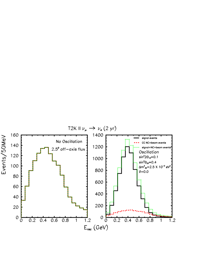
Figure 3: Examples of event number distributions are plotted as a function of the reconstructed neutrino energy for the appearance mode with and without oscillations. In the latter, the following values of the oscillation parameters are used: $\Delta m^{2}_{31}=2.5\times 10^{-3}$ eV², $\sin^{2}\theta_{23}=0.4$, $\sin^{2}2\theta_{13}=0.1$, $\Delta m^{2}_{21}=8.0\times 10^{-5}$ eV², $\sin^{2}\theta_{12}$ = 0.31, $\delta=0$.

Although we do not use the spectrum informations in our analysis, we present in Fig. 3 some examples of the energy distribution of the $\nu_{e}$ appearance events for completeness. For this plot, we set the oscillation parameter $\Delta m^{2}_{31}=2.5\times 10^{-3}$ eV², $\sin^{2}\theta_{23}=0.4$, $\sin^{2}2\theta_{13}=0.1$, $\Delta m^{2}_{21}=8.0\times 10^{-5}$ eV², $\sin^{2}\theta_{12}$ = 0.31, $\delta=0$. Throughout our analysis, we fix the solar neutrino mixing parameters $\Delta m^{2}_{21}$ and $\sin^{2}\theta_{12}$ to these values. One can observe in the figure that background is quite small in size and has similar shape as the signal events. Notice also that the modulation of energy spectrum by neutrino oscillation is rather modest.

IV.2 $\nu_{\mu}\to\nu_{\mu}$ ($\bar{\nu}_{\mu}\to\bar{\nu}_{\mu}$) disappearance mode

The $\nu_{\mu}\to\nu_{\mu}$ ($\bar{\nu}_{\mu}\to\bar{\nu}_{\mu}$) disappearance mode is important to determine $\sin^{2}2\theta_{23}$ as well as $\Delta m^{2}_{31}$ accurately. In Fig. 4, we show the expected event number distribution as a function of the reconstructed neutrino energy in the absence (left panel) and in the presence (right panel) of oscillation with the mixing parameters, $\sin^{2}\theta_{23}=0.4$, $\Delta m^{2}_{23}=2.5\times 10^{-3}$ eV², $\sin^{2}2\theta_{13}=0.1$, and $\delta=0$. Unlike the case of the appearance channel, the energy distribution is significantly modified by the oscillation effect.

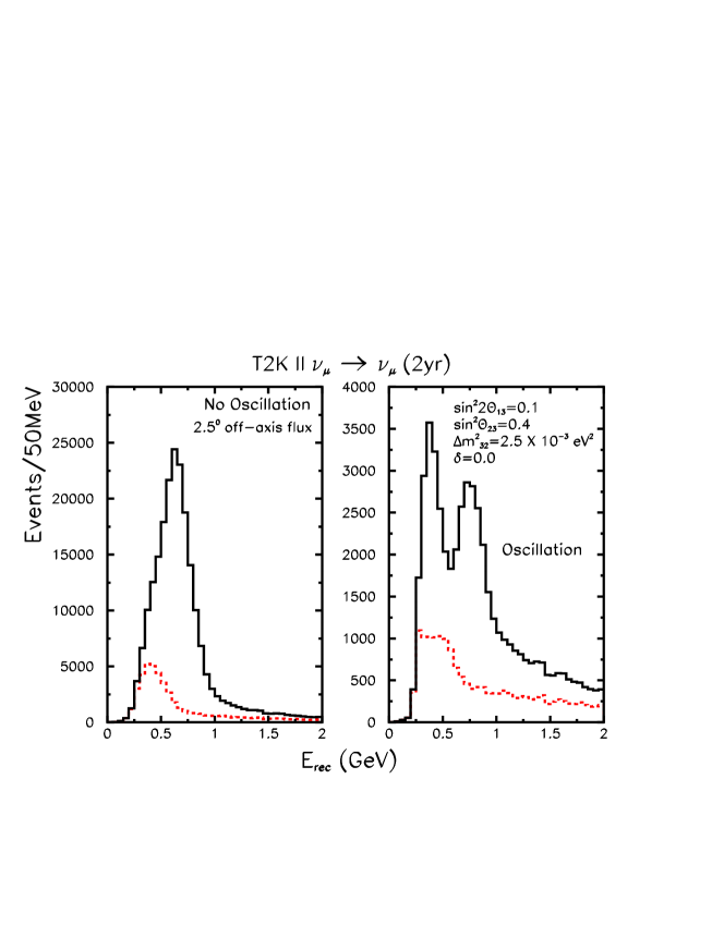
Figure 4: Examples of event number distributions are plotted as a function of the reconstructed neutrino energy for the disappearance mode without oscillation (left panel) and with oscillation (right panel) with the mixing parameters $\Delta m^{2}_{31}=2.5\times 10^{-3}$ eV², $\sin^{2}\theta_{23}=0.4$, $\sin^{2}2\theta_{13}=0.1$, $\Delta m^{2}_{21}=8.0\times 10^{-5}$ eV², $\sin^{2}\theta_{12}$ = 0.31 and $\delta=0$. The histogram by the solid lines indicate the sum of the signal and background events whereas the ones by the dashed line indicate only the background events.

For the disappearance mode, we consider 36 bins with 50 MeV width from 0.2 GeV to 2.0 GeV in terms of the reconstructed neutrino energy. The $\chi^{2}$ function is defined as follows,

$$\chi_{\text{dis}}^{2}\equiv\min_{\alpha_{\text{sig}},\alpha_{\text{BG}}}\sum_{i}\frac{[N_{i}^{\text{obs}}+N_{i,\text{BG}}^{\text{obs}}-(1+\alpha_{\text{sig}})N_{i}^{\text{theo}}-(1+\alpha_{\text{BG}})N_{i,\text{BG}}^{\text{theo}}]^{2}}{N_{i}^{\text{obs}}+N_{i,\text{BG}}^{\text{obs}}}+\left(\frac{\alpha_{\text{sig}}}{\sigma_{\text{sig}}}\right)^{2}+\left(\frac{\alpha_{\text{BG}}}{\sigma_{\text{BG}}}\right)^{2},$$ (15)

where $N_{\text{sig},i}^{\text{obs}}$ and $N_{\text{sig},i}^{\text{theo}}$ are, the number of signal events to be observed and the theoretically expected one, respectively for the $i$-th bin, and $N_{\text{\tiny BG},i}^{\text{obs}}$ and $N_{\text{\tiny BG},i}^{\text{theo}}$ are the corresponding background event numbers. We assume the optimistic values for the systematic errors, $\sigma_{\text{sig}}=\sigma_{\text{BG}}=2$% for the T2K phase II.

In Fig.5, we show the expected sensitivity for $\sin^{2}2\theta_{23}$ assuming the pure 2 flavor oscillation ($\theta_{13}=0$) as a function of the true value of $\Delta m_{23}^{2}$, which compares reasonably well with that of Hiraide . We have checked that this simple $\chi^{2}$ can reproduce the expected T2K sensitivity based on more realistic calculations obtained by Monte Carlo simulation given in Ref. Hiraide .

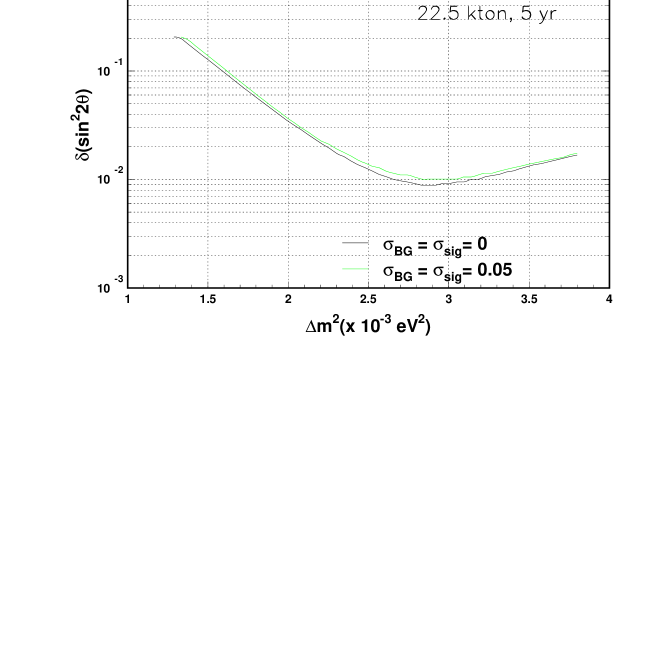
Figure 5: Expected sensitivity on $\sin^{2}2\theta_{23}$ as a function of the true value of $\Delta m^{2}_{23}$ obtained with the $\chi^{2}$ defined in (15) assuming the pure 2 flavor oscillation.

IV.3 $\bar{\nu}_{e}\to\bar{\nu}_{e}$ disappearance mode

For the reactor experiment, we use the same $\chi^{2}$ function used in our previous works reactorCP ; sado , which is defined as,

$$\chi^{2}_{\text{reac}} \equiv \min_{\text{$\alpha$'s}}\sum_{a=f,n}\left[\sum_{i=1}^{17}\left\{\frac{\left(N^{\rm theo}_{ai}-(1+\alpha_{i}+\alpha_{a}+\alpha)N^{\rm obs}_{ai}\right)^{2}}{N^{\rm obs}_{ai}+\sigma_{\rm db}^{2}(N^{\rm obs}_{ai})^{2}}+\frac{\alpha_{i}^{2}}{\sigma_{\rm Db}^{2}}\right\}+\frac{\alpha_{a}^{2}}{\sigma_{\rm dB}^{2}}\right]+\frac{\alpha^{2}}{\sigma_{\rm DB}^{2}},$$ (16)

where $N_{ai}^{\rm theo}$ represents the theoretical number of events at a near ($a=n$) or a far ($a=f$) detector within the $i$-th bin whose width is 0.425 MeV. We set the distance to the near and the far detectors to be 300 m and 1500 m, respectively. $N_{ai}^{\rm obs}$ are number of events to be observed. We consider four types of systematic error: $\sigma_{\rm DB}$, $\sigma_{\rm Db}$, $\sigma_{\rm dB}$ and $\sigma_{\rm db}$. The subscript D (d) represents the fact that the error is correlated (uncorrelated) between detectors. The subscript B (b) represents the fact that the error is correlated (uncorrelated) among bins. The $\alpha$’s are parameters to be varied freely in order to take into account these systematic errors. In this work, we consider the high precision reactor experiments whose sensitivity can go beyond the ones currently expected by experiments such as Double-Chooz DC and KASKA Kaska . Namely, we assume sensitivities below $\sin^{2}2\theta_{13}=0.01$, the one expected to be achievable by phase-II type experiments such as the Braidwood braidwood , the Daya Bay dayabay , and the Angra angra projects.

Computation of the event number is done in the same way as in Ref. sado . We ignore the possible contribution from geo-neutrinos. It is demonstrated recently by KamLAND that its flux is consistent with the one expected by geo-chemical earth models KamLAND_geo . In this case, the effect of geo-neutrinos is negligibly small at the baseline of $\sim$1 km, as one can easily guess by extrapolation of the situation in a reactor $\theta_{12}$ experiment with baseline of $\sim$60 km sado .

To characterize reactor measurement, we use GW$\cdot$kt$\cdot$yr, the “total exposure” unit, which is defined as the product of the net values of the reactor thermal power (in GW), detector fiducial volume (in kton) and running time (in year). We consider the reactor measurement for 10 GW$\cdot$kt$\cdot$yr. The total number of events at the far detector is $1.63\times 10^{6}$. We consider two different sets of systematic errors: a relatively conservative choice and an optimistic one. For the conservative choice, we adopt similar values of the systematic errors used in Ref. reactorCP ; sado , $\sigma_{\rm DB}=\sigma_{\rm Db}=2.0$ % and $\sigma_{\rm dB}=\sigma_{\rm db}=0.5$ %, and for the optimistic one, we set $\sigma_{\rm DB}=\sigma_{\rm Db}=1.0$ % and $\sigma_{\rm dB}=$ 0.2% and $\sigma_{\rm db}=0.2$ %. The latter extremely small errors may be difficult to reach, but they are used to estimate the upper limit of resolving power of the $\theta_{23}$ degeneracy by the present method. The sensitivity limit of $\theta_{13}$ (assuming no depletion) at $\Delta m^{2}_{31}=2.5\times 10^{-3}$ eV² is $\sin^{2}2\theta_{13}=1.14\times 10^{-2}$ ($2.63\times 10^{-2}$) at 1$\sigma$ (3$\sigma$) CL for the relatively conservative errors, and $\sin^{2}2\theta_{13}=5.39\times 10^{-3}$ ($1.25\times 10^{-2}$) at 1$\sigma$ (3$\sigma$) CL for the optimistic ones.

IV.4 Combined analysis

For the combined analysis, we simply sum all the $\chi^{2}$ functions defined in Eqs. (14), (15) and (16),

$$\chi^{2}=\chi_{\text{app}}^{2}+\chi_{\text{dis}}^{2}+\chi_{\text{reac}}^{2}.$$ (17)

The allowed region in the $\sin^{2}2\theta_{13}-\sin^{2}\theta_{23}$ plane is determined by the usual condition, $\Delta\chi^{2}\equiv\chi^{2}-\chi^{2}_{\text{min}}<$ 2.3, 6.18 and 11.83 for 1, 2 and 3 $\sigma$ CL for two degrees of freedom. We will establish the parameter regions where we can resolve the $\theta_{23}$ octant degeneracy for 1 degree of freedom by imposing the condition $|\chi^{2}_{\text{min}}(\theta^{\text{true}}_{23})-\chi^{2}_{\text{min}}(\theta^{\text{false}}_{23})|>$ 2.71, 4 and 6.63 for 90, 95 and 99% CL, respectively, where $\theta^{\text{true}}_{23}$ and $\theta^{\text{false}}_{23}$ are, respectively, the true and the false value of $\theta_{23}$.

V Analysis Results

In this section, we show our results based on our analysis with the combined $\chi^{2}$ of all channels. To remind the readers, our analysis is based on the T2K II experiment of 2 (6) years running of neutrino (anti-neutrino) modes with 4MW beam power with the Hyper-Kamiokande detector whose fiducial volume is 0.54 Mt JPARC . For the reactor experiment, the exposure of 10 GW$\cdot$kt$\cdot$yr is assumed.

We assume throughout this section that the mass hierarchy (determined by nature) is normal type ($\Delta m^{2}_{31}>0$) unless otherwise stated. Even if we repeat the same procedure with the true mass hierarchy of inverted type ($\Delta m^{2}_{31}<0$), the region in which the degeneracy is solved is remarkably similar. Therefore, we decided to concentrate on the normal hierarchy case. Of course, we examine the stability of our results by assuming the wrong hierarchy in the analysis.

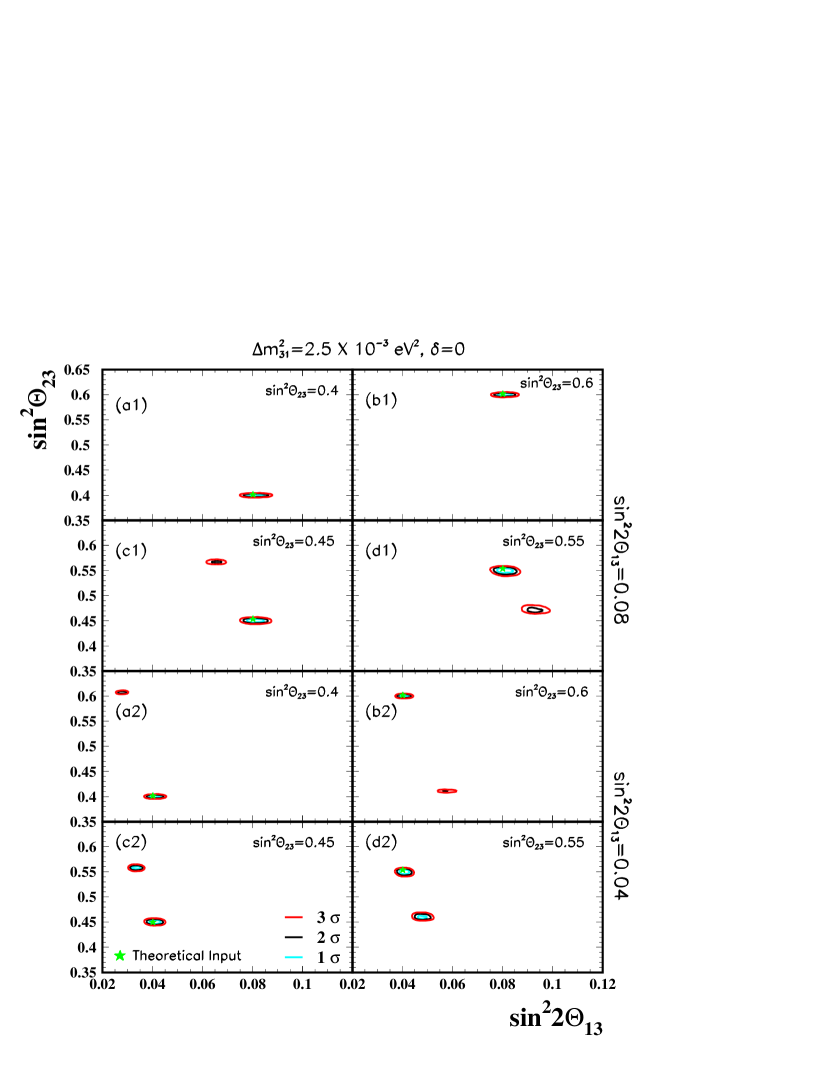
Figure 6: Some examples of the allowed regions in the $\sin^{2}\theta_{13}-\sin^{2}\theta_{23}$ plane determined by the combined analysis for various different input parameters. For all plots, the input values of $\Delta m^{2}_{31}=2.5\times 10^{-3}$eV² and the CP phase $\delta$ = 0. The input value of $\theta_{13}$ for the upper (lower) four panels is $\sin^{2}\theta_{23}=0.08$ (0.04). The input values of $\theta_{23}$ are (a) $\sin^{2}\theta_{23}=0.4$, (b) $\sin^{2}\theta_{23}=0.6$, (c) $\sin^{2}\theta_{23}=0.45$ and (d) $\sin^{2}\theta_{23}=0.55$. The conservative values of the systematic errors are taken for reactor measurement; $\sigma_{\rm DB}=\sigma_{\rm Db}=2.0$ % and $\sigma_{\rm dB}=\sigma_{\rm db}=0.5$ %.

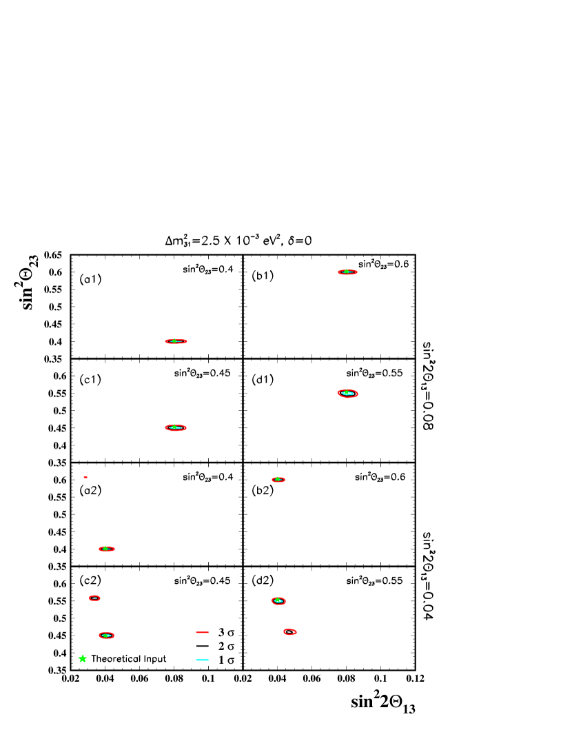
Figure 7: Same as Fig. 6 but for smaller systematic errors for the reactor experiment, $\sigma_{\text{DB}}=\sigma_{\text{Db}}=1$ %, $\sigma_{\text{db}}=0.2$ % and $\sigma_{\text{dB}}=0.2$ %.

In Fig. 6, we show the allowed regions in the $\sin^{2}2\theta_{13}-\sin^{2}\theta_{23}$ plane at 1 $\sigma$ (light blue curve), 2 $\sigma$ (black curve), and 3 $\sigma$ (red curve) CL for 2 degree of freedom, for 8 different sets of input parameters; $(\sin^{2}2\theta_{13},\sin^{2}\theta_{23})$ = (0.08, 0.4), (0.08, 0.6), (0.08, 0.45), (0.08, 0.55), (0.04, 0.4), (0.04, 0.6) and (0.04, 0.45), (0.04, 0.55), which are indicated by the symbol of a star. They are determined by the combined $\chi^{2}$ analysis using all the channels, $\nu_{\mu}\to\nu_{e}$ ($\bar{\nu}_{\mu}\to\bar{\nu}_{e}$) appearance mode, by $\nu_{\mu}\to\nu_{\mu}$ ($\bar{\nu}_{\mu}\to\bar{\nu}_{\mu}$) disappearance mode and by $\bar{\nu}_{e}\to\bar{\nu}_{e}$ disappearance mode. The relatively conservative values of the systematic errors are taken for the reactor measurement; $\sigma_{\rm DB}=\sigma_{\rm Db}=2.0$ % and $\sigma_{\rm dB}=\sigma_{\rm db}=0.5$ %. In our $\chi^{2}$ analysis, for given values of input parameters, we vary not only $\theta_{23}$ and $\theta_{13}$ but also $\delta$ and $\Delta m^{2}_{31}$, as these parameters should be determined by the fit. Note, however, that the range of $\Delta m^{2}_{31}$ and $\theta_{23}$ are restricted to the ones constrained by atmospheric neutrino experiments SKatm .

For a larger value of $\sin^{2}2\theta_{13}=0.08$, the octant degeneracy is resolved for $\sin^{2}2\theta_{23}=0.96$ (see Fig. 6a1 and b1), whereas for $\sin^{2}2\theta_{23}=0.99$, the degeneracy can be resolved only at 1 $\sigma$ CL but not at 2 $\sigma$ CL or higher (see Fig. 6c1 and d1). For a smaller value of $\sin^{2}2\theta_{13}=0.04$, for $\sin^{2}2\theta_{23}=0.96$, the octant degeneracy is resolved only at 1 $\sigma$ CL (see Fig. 6a2 and b2) and for $\sin^{2}2\theta_{23}=0.99$, the degeneracy can not be resolved even at 1 $\sigma$ CL (see Fig. 6c2 and d2).

In Fig. 7, we show the same quantities but for the small systematic errors for reactor experiments, $\sigma_{\text{DB}}=\sigma_{\text{Db}}=1$ %, $\sigma_{\text{db}}=\sigma_{\text{dB}}=0.2$ %, the very optimistic ones. In this case, the octant degeneracy is completely resolved for a large $\theta_{13}$, $\sin^{2}2\theta_{13}=0.08$ both for $\sin^{2}2\theta_{23}=0.96$ and 0.99 (see Fig. 7a1, b1, c1, and d1). For a small value of $\theta_{13}$, $\sin^{2}2\theta_{13}=0.04$, however, we have a mixed result; For $\sin^{2}2\theta_{23}=0.96$, the $\theta_{23}$ degeneracy is resolved both for $\sin^{2}2\theta_{23}=0.96$ and 0.99 apart from a tiny 3$\sigma$ CL region in Fig. 7a2. For $\sin^{2}2\theta_{23}=0.99$, the degeneracy is not lifted, except in Fig. 7d2 where the clone solution disappears at 1$\sigma$ CL.

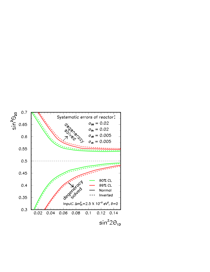
Figure 8: The region in $\sin^{2}2\theta_{13}-\sin^{2}\theta_{23}$ space where the $\theta_{23}$ octant degeneracy can be resolved at 90% (thin green) and 99% (thick red) CL. The solid (dashed) curve is for the case of taking the normal (inverted) hierarchy to perform the fit, assuming the normal hierarchy as input. Conservative systematic errors, as indicated in the figure, are considered here.

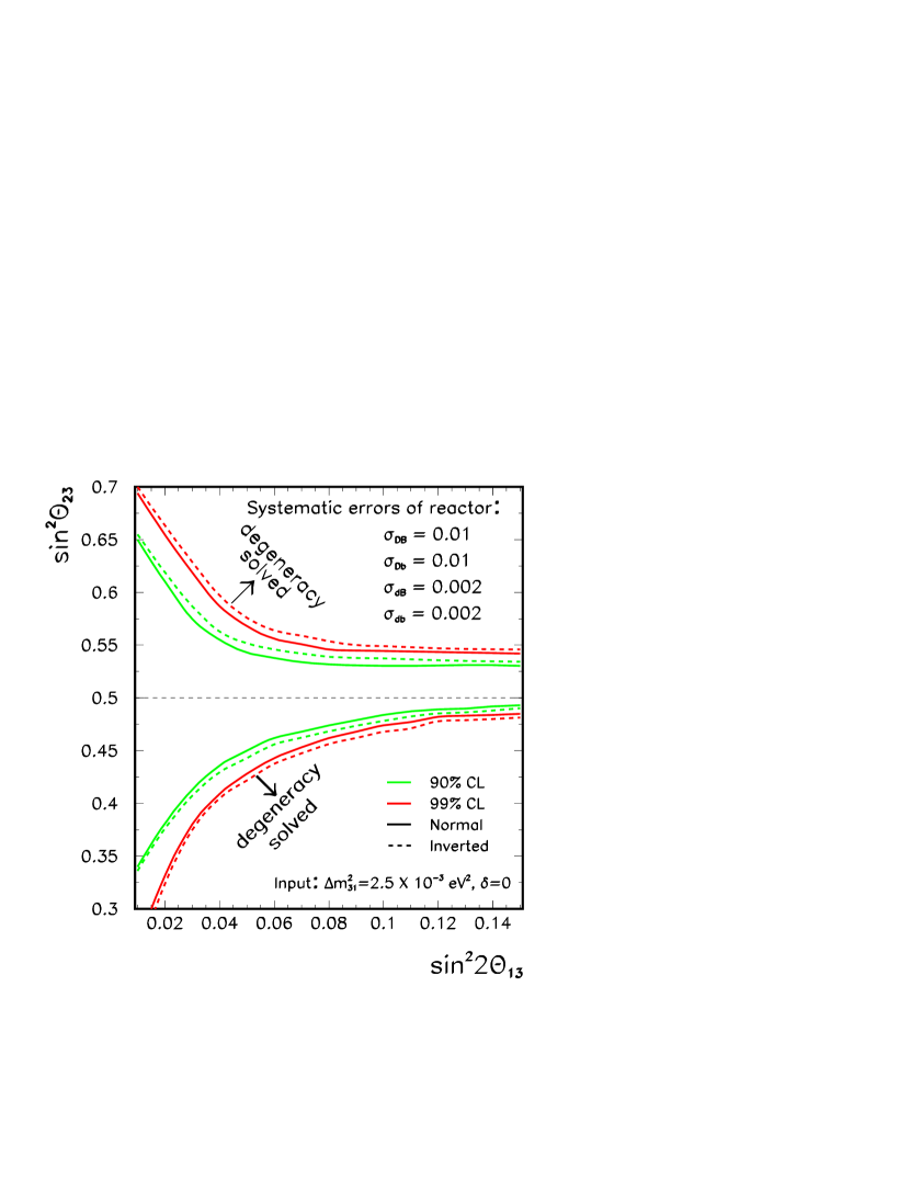
Figure 9: The same as in Fig. 8 but with optimistic systematic errors.

In Fig. 8 and Fig. 9, we show the region bounded by the solid and the dashed curves in which we can resolve the $\theta_{23}$ octant degeneracy in the $\sin^{2}\theta_{13}$-$\sin^{2}\theta_{23}$ plane at 90% (thin green curves) and 99% (thick red curves) CL for 1 degree of freedom for the conservative and the optimistic values of the reactor systematic errors, respectively. Namely, the region inside the bands correspond to the parameters which satisfies $|\chi^{2}_{\text{min}}(\theta^{\text{true}}_{23})-\chi^{2}_{\text{min}}(\theta^{\text{false}}_{23})|>$ 2.71 and 6.63 where $\theta^{\text{true}}_{23}$ and $\theta^{\text{false}}_{23}$ are the true and the false values of $\theta_{23}$, respectively. The solid (dashed) curves in Fig. 8 and Fig. 9 are for cases that we fit the data set generated with $\Delta m^{2}_{31}>0$ under the hypothesis of right hierarchy, $\Delta m^{2}_{31}>0$ (wrong hierarchy, $\Delta m^{2}_{31}<0$). If we are ignorant about the mass hierarchy the case of worse sensitivity (wrong hierarchy) must be considered as the sensitivity region. The fact that the solid and the dashed curves come close to each others proves that the resolution of the $\theta_{23}$ octant degeneracy can be carried out independent of the lack of knowledge on the neutrino mass hierarchy, the decoupling of the two degeneracies as argued in Sec. III.5.

The figures indicate that our method of combining reactor measurement of $\theta_{13}$ with the accelerator disappearance and appearance experiments allows to resolve the $\theta_{23}$ octant degeneracy to a reasonable level. This is highly nontrivial because it is quite a robust degeneracy which is hard to lift by using only relatively short-baseline ($\sim 1000$ km) accelerator measurement, as we saw in Sec. III. We can observe by comparison between Fig. 8 and Fig. 9 that improvement of the systematic errors in reactor measurement is the key to the better resolving power of the octant degeneracy. It should also be mentioned that the results in Fig. 9 are obtained with the extremely small systematic errors. Hence, the results may be interpreted as the limit achievable by the present method.

So far we have assumed that the input mass hierarchy is normal while examining the true and the false mass hierarchies in analyzing data. In order to verify that resolving power of $\theta_{23}$ degeneracy is not affected by the unknown sign of $\Delta m^{2}_{31}$, we tried the converse. Namely, we tried to fit the data set generated with the inverted hierarchy $\Delta m^{2}_{31}<0$ under the hypothesis of the right and the wrong hierarchies. We do not show the results because they are very similar to those for the input normal mass hierarchy. Of course, this is expected because the experimental setting we consider in this work is not sensitive to the sign of $\Delta m^{2}_{31}$, which in turn implies that our results must be insensitive to the mass hierarchy confusion. This point was discussed in depth in Sec. III.

We note that globally our results in Fig. 8 and Fig. 9 are similar to what we can find in Fig.7 of Ref. MSYIS , which was obtained by a much more simplified analysis. However, there are some notable differences. In Fig.7 of Ref. MSYIS , it is always true that the $\theta_{23}$ degeneracy is easier to lift in the second octant, $\theta_{23}>\pi/4$. But, we observe that it is true only for relatively small $\theta_{13}$, $\sin^{2}2\theta_{13}\raise 1.29167pt\hbox{$\;<$\kern-7.5pt\raise-4.73611pt\hbox{$\sim\;$}}0.06$. For relatively large $\theta_{13}$, $\sin^{2}2\theta_{13}\raise 1.29167pt\hbox{$\;>$\kern-7.5pt\raise-4.73611pt\hbox{$\sim\;$}}0.06$, the octant degeneracy is easier to be resolved for the first octant case $\theta_{23}<\pi/4$ than for the second octant.

It appears that at large $\theta_{13}$, the two effects which were not taken into account in the treatment in MSYIS come into play, as indicated in Fig. 1; The width of the appearance strip, which comes from $\delta$-dependent terms in the oscillation probability (see Eq. (8) in Sec. III.2), is narrower at smaller $\theta_{13}^{\rm fake}$, which is the case of true $\theta_{23}$ in the first octant, making rejection of the fake solution easier. Also, the two disappearance “lines” come closer in the case of true $\theta_{23}$ in the second octant, which produces the similar effect. As a result of the two effects which simultaneously act toward the same direction, the degeneracy turns out to be easier to resolve for the case of true $\theta_{23}$ in the first octant. We, however, want to note that the feature of first-second octants asymmetry, in particular in Fig. 8, depends upon the systematic errors and its full understanding may require much more subtle discussions.

VI Concluding remarks

In this paper, we have explored the possibility of resolving the $\theta_{23}$ octant degeneracy by combining reactor measurement of $\theta_{13}$ with the possible highest accuracy accelerator disappearance and appearance measurement, as proposed in MSYIS . It utilizes the nature of the reactor experiment as a pure measurement of $\theta_{13}$ to resolve the degeneracy. It is nice to see that the reactor measurement can contribute to explore the two small quantities in lepton flavor mixing, $\theta_{13}$ and a deviation of $\theta_{23}$ from the maximal value. The results of our quantitative analysis indicates reasonably high performance of the method. As shown in the summary figures of the resolving capabilities, Fig. 8 and Fig. 9, the degeneracy is resolved in region of relatively large $\theta_{13}$ and a sizable deviation of $\theta_{23}$ from the maximal.

Prior to the quantitative analysis based on our method, we have discussed the robustness of the $\theta_{23}$ octant degeneracy and illuminated the difficulty in resolving it only by accelerator experiments. In particular, we have demonstrated by showing a sample figure, Fig. 2, that neither the spectral information nor the matter effect enables us to resolve the degeneracy, This feature was also understood on the basis of analytic treatment using the approximate formulas for appearance and disappearance probabilities valid to first order in matter effect. Considering the robustness of the degeneracy, the opportunity of resolution offered by our reactor-accelerator method is highly nontrivial.

Finally, several remarks are in order:

(1) As indicated in Fig. 1, the sensitivity of our method for resolving the $\theta_{23}$ degeneracy is limited mainly by the accuracy of $\theta_{13}$ determination by reactor experiments. The region without resolving power which remains in Fig. 9 must be taken as the intrinsic limitation of our method for resolving the $\theta_{23}$ degeneracy in its current form, because we have already assumed a rather optimistic values of systematic errors in the reactor measurement, in addition to the extreme accuracies of accelerator experiments.

(2) In this paper, we have considered the setting of T2K experiment originally described in JPARC . It would be interesting to examine how the sensitivity of resolution of $\theta_{23}$ degeneracy changes if we adopt the Kamioka-Korea identical two-detector setting by which the degeneracy related to the neutrino mass hierarchy and the intrinsic one can be resolved T2KK .

(3) Our method for resolving $\theta_{23}$ degeneracy is by no means unique. The other possibilities include: accelerator measurement with silver channel ($\nu_{e}\rightarrow\nu_{\tau}$) silver which has a different $\theta_{23}$ dependence, and detection of the solar oscillation term by either atmospheric neutrino observation, atm23 ; concha-smi_23 ; choubey2 or very long baseline accelerator experiments BNL . Combination of the accelerator and the atmospheric neutrino experiments can also be pursuit atm-lbl . The ultimate possibility would, of course, be the “everything at once” approach donini which combines measurement by superbeam and neutrino factories with golden and silver channels.

Appendix A Calculation of Number of Events

In this appendix, we provide some detailed informations about how the number of events are computed. For clarity of notation we denote the neutrino energy ($E$ in the text) as $E_{\nu}$ in this appendix.

(i) Apparence channel $\nu_{\mu}\to\nu_{e}$ (or $\bar{\nu}_{\mu}\to\bar{\nu}_{e}$) As we mentioned in sec. IV, since the information on the energy spectrum of the appearance channel is not important in resolving $\theta_{23}$ degeneracy, for this channel, we do not try to make binning but use the expected total number of events, which is computed as,

$$N_{\rm sig}=n_{N}T\int_{E_{\nu}^{\rm min}}^{E_{\nu}^{\text{max}}}dE_{\nu}\phi_{\nu_{\mu}}(E_{\nu})P(\nu_{\mu}\to\nu_{e};E_{\nu})\sigma^{\nu_{e}}_{\rm tot}(E_{\nu})\epsilon_{\nu_{e}}(E_{\nu}),$$ (18)

where $E_{\nu}$ is the (true) neutrino energy, $n_{N}$ is the number of target nucleons in the detector, $T$ is the running (exposure) time, $\phi_{\nu_{\mu}}(E_{\nu})$ is the flux spectrum of the 2.5 degree off axis $\nu_{\mu}$ beam $\sigma^{\nu_{e}}_{\rm tot}(E_{\nu})$ is the total cross section and $\epsilon_{\nu_{e}}(E_{\nu})$ is the detection efficiency, which is given as a function of the neutrino energy. The detection efficiency we used takes into account all the cut imposed to reduce background, which enables us to obtain the signal distribution in the range between 0.35 and 0.85 GeV in terms of reconstructed neutrino energy JPARC-detail .

We consider two kinds of background events,

$$N_{\rm total}^{\rm BG}=N_{\rm total}^{\rm BG(NC)}+N_{\rm total}^{\rm BG(beam)},$$ (19)

where $N_{\rm total}^{\rm BG(NC)}$ comes from neutral current interactions and $N_{\rm total}^{\rm BG(beam)}$ implies the event induced by the $\nu_{e}$ neutrino existed in the original beam. As for the signal, we used the efficiency functions which correspond to the cuts found in Ref. JPARC-detail in order to compute the background.

(ii) Disapparence channel $\nu_{\mu}\to\nu_{\mu}$ (or $\bar{\nu}_{\mu}\to\bar{\nu}_{\mu}$) For the disappearance mode, it is essential to make binning in order to take into account the information on the energy spectrum. The expected number of signal events for the i-th bin is computed as follows

$$N_{\rm sig,i}=n_{N}T\int_{E_{\rm rec}^{\rm i;min}}^{E_{\rm rec}^{\text{i; max}}}dE_{\rm rec}\int_{E_{\nu}^{\text{min}}}^{E_{\nu}^{\text{max}}}dE_{\nu}\phi_{\nu_{\mu}}(E_{\nu})P(\nu_{\mu}\to\nu_{\mu};E_{\nu})\sigma^{\nu_{\mu}}_{\rm CCQE}(E_{\nu})\epsilon^{\rm rec}_{\nu_{\mu}}(E_{\rm rec})R(E_{\nu},E_{\rm rec}),$$ (20)

where $E_{\rm rec}$ implies reconstructed neutrino energy, $\sigma^{\nu_{\mu}}_{\rm CCQE}(E_{\rm rec})$ implies charged current quasi elastic (CCQE) reaction cross section, $\epsilon^{\rm rec}_{\nu_{\mu}}(E_{\rm rec})$ is the detection efficiency as a function of the reconstructed neutrino energy, which corresponds to the one used in Ref. Hiraide , $R(E_{\nu},E_{\rm rec})$ is the Gaussian-like resolution function,

$$R(E_{\nu},E_{\rm rec})=\frac{1}{\sqrt{2\pi}\sigma_{E}}\text{exp}\left[-\frac{1}{2}\left(\frac{E_{\nu}-E_{\rm rec}}{\sigma_{E}}\right)^{2}\right],$$ (21)

where we set $\sigma_{E}$ = 80 MeV.

For this mode, we consider two kinds of background,

$$N_{i}^{\rm BG}=N_{i}^{\rm BG(NC)}+N_{i}^{\rm BG(CC-NQE)},$$ (22)

where $N_{i}^{\rm BG(NC)}$ is the events coming from neutral current reaction and $N_{i}^{\rm BG(CC-NQE)}$ is the one coming from the charged current non-quasi elastic (CC-NQE) reactions. We note that $N_{i}^{\rm BG(NC)}$ do not depend on oscillation parameters, whereas $N_{i}^{\rm BG(CC-NQE)}$ depend on oscillation parameters in a non-trivial way. For the background coming from CC-NQE reactions, $E_{\rm rec}=E_{\rm true}$ is not a good approximation because events induced by higher energy neutrinos mimic the signal induced by lower energy ones. However, we observe that it is a good approximation to take that $E_{\rm rec}-E_{\rm true}=300$ MeV or $N_{i}^{\rm BG(CC-NQE)}(E_{\rm rec})\simeq N_{i}^{\rm BG(CC-NQE)}(300\ {\rm MeV}+E_{\rm true})$. This allows us to compute $N_{i}^{\rm BG(CC-NQE)}(E_{\rm rec})$ in the presence of oscillation provided that we know the distribution $N_{i}^{\rm BG(CC-NQE)}$ as a function of reconstructed neutrino energy in the absence of oscillation for the 2.5 degree beam.

(iii) Disappearance channel $\bar{\nu}_{e}\to\bar{\nu}_{e}$ We compute the expected number of $\bar{\nu}_{e}$ events in the $i$-th energy bin, $N_{i}^{\text{theo}}=N_{i}^{\text{reac}}$, where $N_{i}^{\text{reac}}$

$$N_{i}^{\text{reac}}(\sin^{2}\theta_{12},\Delta m^{2}_{21}) = N_{p}T$$

$$\times\int dE_{\nu} \,\epsilon\phi(E_{\nu})P(\bar{\nu}_{e}\to\bar{\nu}_{e};L,E_{\nu})\sigma(E_{\nu})\int_{i}dE\epsilon_{\text{det}}\,R(E,E^{\prime}),$$ (23)

where $N_{p}$ is the number of target protons in the detector fiducial volume, $T$ is the exposure time, and $\phi(E_{\nu})$ is the neutrino flux spectrum from the nuclear power plant (NPP) expected at its maximal thermal power operation. $\epsilon$ denotes the averaged operation efficiency of the NPP for a given exposure period and it is taken to be 100% here under the understanding that the unit we use GW${}_{\text{th}}\cdot$kt$\cdot$yr refers the actual thermal power generated, not the maximal value. $P(\bar{\nu}_{e}\ \to\bar{\nu}_{e},L,E_{\nu})$ is the familiar antineutrino survival probability in vacuum, which is given by Eq.(5) and it explicitly depends on $\Delta m^{2}_{21}$ and $\sin^{2}\theta_{12}$. $\sigma(E_{\nu})$ is the $\bar{\nu}_{e}$ absorption cross-section on proton, $\epsilon_{\text{det}}=0.898$ is the detector efficiency and $R(E,E^{\prime})$ is the energy resolution function, which is assumed to have a Gaussian form with $E$ ($=E_{\text{prompt}})$ the observed prompt energy (total $e^{+}$ energy) and $E^{\prime}=E_{\nu}$ - 0.8 MeV the true one.