Solar neutrino oscillation parameters
after first KamLAND results

Abstract

We analyze the energy spectrum of reactor neutrino events recently observed in the Kamioka Liquid scintillator Anti-Neutrino Detector (KamLAND) and combine them with solar and terrestrial neutrino data, in the context of two- and three-family active neutrino oscillations. In the $2\nu$ case, we find that the solution to the solar neutrino problem at large mixing angle (LMA) is basically split into two sub-regions, that we denote as LMA-I and LMA-II. The LMA-I solution, characterized by lower values of the squared neutrino mass gap, is favored by the global data fit. This picture is not significantly modified in the $3\nu$ mixing case. A brief discussion is given about the discrimination of the LMA-I and LMA-II solutions with future KamLAND data. In both the $2\nu$ and $3\nu$ cases, we present a detailed analysis of the post-KamLAND bounds on the oscillation parameters.

I Introduction

The year 2002 is likely to be remembered as the annus mirabilis of solar neutrino physics. On April 20, direct and highly significant evidence for $\nu_{e}$ flavor change into active states was announced by the Sudbury Neutrino Observatory (SNO) experiment AhNC , crowning a four-decade long Deca series of beautiful observations Cl98 ; Ksol ; Ab02 ; Ha99 ; Ki02 ; Fu01 ; Fu02 ; AhCC ; AhDN of the solar $\nu_{e}$ flux deficit Ba89 ; BP00 . On October 8, the role of solar neutrino physics in shaping modern science was recognized through the Nobel Prize jointly awarded to Raymond Davis, Jr., and Masatoshi Koshiba, for their pioneering contributions to the detection of cosmic neutrinos Nobe . Finally, on December 6, clear “terrestrial” evidence for the oscillation solution to the solar neutrino deficit was reported by the Kamioka Liquid scintillator AntiNeutrino Detector (KamLAND), through the observation of long-baseline reactor $\overline{\nu}_{e}$ disappearance Kam1 . The seminal idea of studying lepton physics by detecting solar Po46 ; Al49 and reactor Po46 ; Al49 ; Re53 neutrinos keeps thus bearing fruits after more than 50 years.

The KamLAND observation of $\overline{\nu}_{e}$ disappearance Kam1 confirms the current interpretation of solar neutrino data AhDN ; Fu02 ; AllS ; GetM ; Las3 in terms of $\nu_{e}\to\nu_{\mu,\tau}$ oscillations induced by neutrino mass and mixing Pont ; Maki , and restricts the corresponding parameter space $(\delta m^{2},\theta_{12})$ within the so-called large mixing angle (LMA) region. In this region, globally favored by solar neutrino data Smir , matter effects Matt ; Barg in adiabatic regime Adia ; Matt are expected to dominate the dynamics of flavor transitions in the Sun (see, e.g., LasA ). The KamLAND spectral data appear to exclude some significant portions of the LMA solution Kam1 , where the predicted spectrum distortions Mu02 ; Marf ; Barb ; Go01 ; Vi02 ; GoKL ; Al02 ; Ho02 ; Go02 ; Las3 would be in conflict with observations Kam1 .

In this paper we analyze the first KamLAND spectral data Kam1 and combine them with current solar neutrino data Cl98 ; Ab02 ; Ha99 ; Ki02 ; Fu02 ; AhNC ; AhCC ; AhDN , assuming two- and three-flavor oscillations of active neutrinos Las3 , in order to determine the surviving sub-regions of the LMA solution. In the analysis we include the CHOOZ reactor data CHOO and, in the $3\nu$ case, also the relevant constraints on the larger mass gap $\Delta m^{2}\gg\delta m^{2}$, coming from the Super-Kamiokande (SK) atmospheric Shio and KEK-to-Kamioka (K2K) accelerator K2Ke ; K2Ks neutrino experiments, according to the approach developed in Las3 .

In the $2\nu$ case, we find that the inclusion of the KamLAND spectrum basically splits the LMA solution into two sub-regions at “small” and “large” $\delta m^{2}$, which we call LMA-I and LMA-II, respectively (the LMA-I solution being preferred by the data). Such regions are only slightly modified in the presence of $3\nu$ mixing, namely, for nonzero values of the mixing angle $\theta_{13}$. We also present updated bounds in the $3\nu$ parameter space $(\delta m^{2},\theta_{12},\theta_{13})$.

The structure of this paper is as follows. In Sec. II we describe our analysis of the KamLAND data. In Sec. III we combine such measurements with solar and CHOOZ data, assuming $2\nu$ mixing. In Sec. IV we extend the analysis to $3\nu$ mixing, including the SK+K2K terrestrial neutrino constraints. We draw our conclusions in Sec. V.

II Kamland data input

In our KamLAND data analysis, we use the absolute spectrum of events reported in Kam1 , taken above a background-safe analysis threshold of 2.6 MeV in visible energy $E$. The events below such threshold might contain a significant component of geological $\overline{\nu}_{e}$’s GeoN , whose large normalization uncertainties are poorly constrained at present by the KamLAND data themselves Kam1 . Above 2.6 MeV, a total of 54 events is found (including at most one possible background candidate), against 86.8 events expected from reactors Kam1 .

The observed energy spectrum of events is analyzed as in Las3 , with the following improvements. According to Kam1 , we adopt: (1) Relative fuel components ²³⁵U : ²³⁸U : ²³⁹Pu : ²⁴¹Pu = 0.568 : 0.078 : 0.297 : 0.057; (2) Absolute normalization of 86.8 events for no oscillations; (3) Energy resolution width equal to $7.5\%/E^{1/2}$; (4) Thirteen bins in visible energy above 2.6 MeV, with 0.425 MeV width. The experimental and theoretical (oscillated) number of events in each bin are denoted as $N_{i}^{\mathrm{expt}}$ and $N_{i}^{\mathrm{osc}}$, respectively $(i=1,\dots,13)$.

Concerning the systematic errors, the information in Kam1 does not allow to trace the magnitude and the bin-to-bin correlations of each component. We have then approximately grouped such uncertainties into two main components, labelled by the index $k=1,\,2$: (1) energy scale error; and (2) overall normalization error. The first (second) uncertainty basically shifts the spectrum along the energy (event) coordinate. More precisely, the effect of the energy scale error $(k=1)$ is estimated by taking the (symmetrized) fractional differences $c^{1}_{i}$ between the values of $N_{i}^{\mathrm{osc}}$ calculated with and without shifts of $\pm 1.91\%$ Kam1 in the true visible energy, for each point in the oscillation parameter space. The normalization uncertainty $(k=2)$ is here assumed to collect all the other error components listed in Kam1 , up to a total of about 6%: $c^{2}_{i}=0.06$. The systematic shifts $c^{k}_{i}$ of the $N_{i}^{\mathrm{osc}}$’s are then implemented through the “pull approach” described in GetM , namely, through linear deviations $N_{i}^{\mathrm{osc}}\to N_{i}^{\mathrm{theo}}=N_{i}^{\mathrm{osc}}(1+\sum_{k}c^{k}_{i}\xi_{k})$, where the $\xi_{k}$’s are univariate Gaussian random variables. In this way, systematic correlations are also accounted for GetM .

Concerning the statistical errors, the presence of bins with few or zero events requires Poisson statistics, that we approximately implement through the $\chi^{2}$-like recipe suggested in the Review of Particle Properties PDGr . A quadratic penalty in the pulls $\xi_{k}$ is introduced to account for the systematics GetM ; Lind . The final $\chi^{2}$ function for KamLAND (KL) is thus

$$\chi^{2}_{\mathrm{KL}}=\min_{\{\xi_{k}\}}\left[\sum_{i=1}^{13}2\left(N_{i}^{\mathrm{theo}}-N_{i}^{\mathrm{exp}}+N_{i}^{\mathrm{exp}}\ln\frac{N_{i}^{\mathrm{exp}}}{N_{i}^{\mathrm{theo}}}\right)+\sum_{k=1,2}\xi^{2}_{k}\right]\ ,$$ (1)

where the $i$-th logarithmic term is dropped if $N_{i}^{\mathrm{exp}}=0$ PDGr . By expanding the first sum in the $\chi^{2}$ at first order in the shifts $c^{k}_{i}$, the minimization in Eq. (1) becomes elementary.

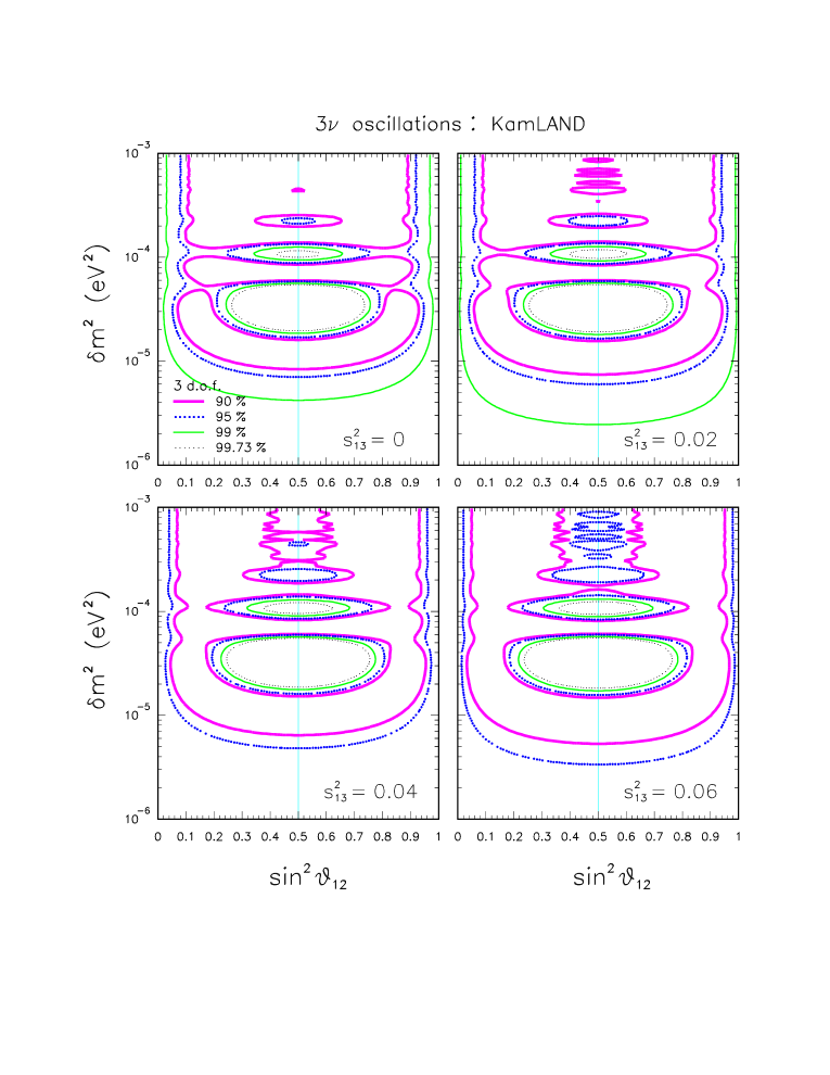
Figure 6: Three-flavor active neutrino oscillations: Global analysis of KamLAND data, shown in the same format as Fig. 5. Notice the enlargement of the allowed regions for increasing $s^{2}_{13}$.

Some final remarks are in order. A detailed comparison of the above function $\chi^{2}_{\mathrm{KL}}$ with the one adopted by the KamLAND collaboration is not currently possible, since the latter is given in a symbolic form in Kam1 . However, one can observe that: (1) The KamLAND collaboration splits the total rate and spectrum shape information, while we prefer to use the absolute spectrum; (2) The KamLAND collaboration can take into account a (very small) background component above 2.6 MeV and four sources of systematics while, for a lack of information, we neglect such small background, and group the systematics into two main sources. For such reasons, we do not expect perfect quantitative agreement between the KamLAND official oscillation analysis and ours. In fact, we find that the 95% C.L. contours of the rate+shape analysis in Fig. 6 of Kam1 are accurately reproduced by our Eq. (1) at a slightly lower C.L. ($90\%$). This loss of statistical power appears tolerable to us, in the light of the limited experimental information which is currently available.

III $2\nu$ analysis

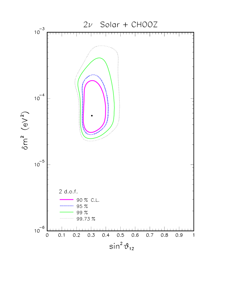
Figure 1: Two-flavor active neutrino oscillations: Global analysis of solar and CHOOZ neutrino data in the $(\delta m^{2},\sin^{2}\theta_{12})$ parameter space, restricted to the LMA region. The best fit is indicated by a black dot. The 90, 95, 99, and 99.73% C.L. contours correspond to $\Delta\chi^{2}=4.61$, 5.99, 9.21, and 11.83, respectively (two degrees of freedom). For solutions at lower $\delta m^{2}$—now ruled out by KamLAND—see Las3 .

The updated $2\nu$ analysis of current solar+CHOOZ neutrino data, as performed in Las3 , is presented here for the sake of completeness. The fit includes 81 solar neutrino observables GetM ; Las3 and 14 CHOOZ spectrum bins CHOO ; Las3 , for a total of 95 data points. The best-fit point and its $\chi^{2}_{\mathrm{\min}}$ value are given in the first row of Table I. The $\Delta\chi^{2}$ expansion around the minimum, relevant for the estimation of the oscillation parameters $(\delta m^{2},\sin^{2}\theta_{12})$, is shown in Fig. 1, where we have restricted the $\delta m^{2}$ range to the only three decades relevant for the LMA solution and for the following KamLAND analysis. Notice that the scale is linear in the $\sin^{2}\theta_{12}$ variable.

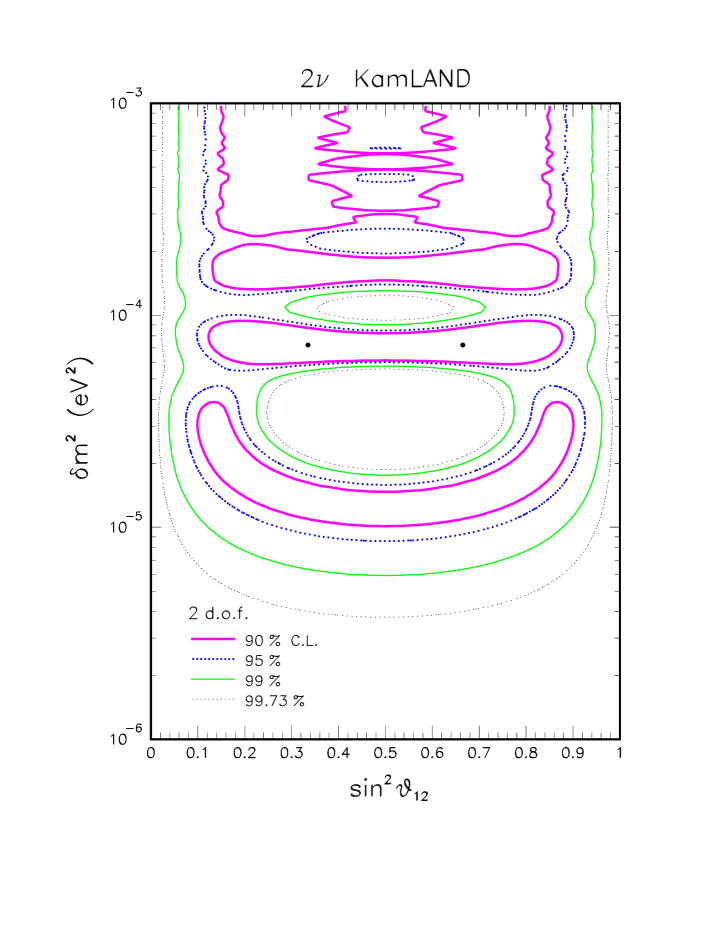
Figure 2: Two-flavor active neutrino oscillations: Analysis of the KamLAND energy spectrum data above 2.6 MeV in the $(\delta m^{2},\sin^{2}\theta_{12})$ parameter space. A “tower” of octant-symmetric regions is allowed at different values of $\delta m^{2}$. The three lower regions with $\delta m^{2}\lesssim 2\times 10^{-4}$ eV² are well separated at 90% C.L., while the upper ones tend to merge in a continuum. The symmetric best fits are indicated by black dots. The left dot is remarkably close to the solar best fit in Fig. 1.

The $2\nu$ analysis of KamLAND is performed by using Eq. (1), which gives the absolute $\chi^{2}_{\mathrm{min}}$ value reported in the second row of Table I. For later purposes, we also quote the second best fit parameters. Expansion around the absolute minimum gives the C.L. contours shown in Fig. 2. There appears to be a “tower” of solutions which tend to merge and become indistinguishable for increasing $\delta m^{2}$; the lower three ones are, however, rather well separated at 90% C.L. Notice that our allowed regions are slightly larger (i.e., less constraining) than those in the rate+shape analysis of Kam1 , as explained in Sec. II. One of the two octant-symmetric best fits points in Fig. 2 (black dots) is remarkably close to the best fit in Fig. 1 (see also Table I). The difference in location with respect to the KamLAND official best-fit point at $(\delta m^{2}/\mathrm{eV}^{2},\sin^{2}\theta_{12})=(6.9\times 10^{-5},\,0.5)$ Kam1 is not statistically significant, amounting to a variation $\Delta\chi^{2}\ll 1$.

Table 1: Results of the two-flavor oscillation analysis. The first two columns report the data set used and the corresponding number of data point $N_{\mathrm{data}}$, respectively. The third and fourth columns give the position and $\chi^{2}_{\min}$ value of the first and second best fit point (when applicable). For a goodness-of-fit check, the $\chi^{2}_{\min}$ value should be compared with its expected $\pm 1\sigma$ range, given by $[N_{\mathrm{DF}}-\sqrt{2N_{\mathrm{DF}}},N_{\mathrm{DF}}+\sqrt{2N_{\mathrm{DF}}}]$ PDGr , where $N_{\mathrm{DF}}=N_{\mathrm{data}}-2$ (see last column). All the $\chi^{2}_{\mathrm{min}}$ values appear to be close to—or slightly below—the lower end of such $\pm 1\sigma$ range, indicating that the fits are somewhat better than statistically expected (although not suspiciously so).

Experimental data set	No. of data	Best fit point(s)	$\chi^{2}_{\min}$	$N_{\mathrm{DF}}\pm\sqrt{2N_{\mathrm{DF}}}$
Solar+CHOOZ	81+14	(5.5, 0.305)	78.8	[79.4, 106.6]
KamLAND	13	(7.3, 0.335)	6.1	[6.3, 15.7]
	13	(18.0, 0.270)	7.9	[6.3, 15.7]
Solar+CHOOZ+KamLAND	81+14+13	(7.3, 0.315)	85.2	[91.4, 120.6]
	81+14+13	(15.4, 0.300)	90.6	[91.4, 120.6]

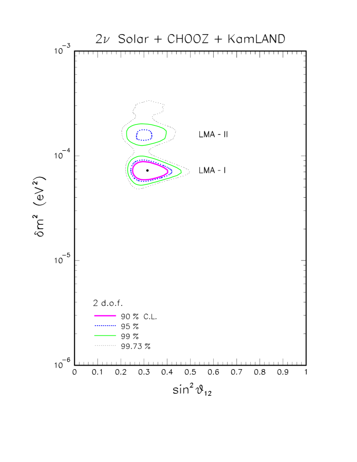
Figure 3: Two-flavor active neutrino oscillations: Global analysis of solar, CHOOZ, and KamLAND neutrino data in the $(\delta m^{2},\sin^{2}\theta_{12})$ parameter space. With respect to Fig. 1, the LMA region is significantly restricted, and appears to be split into two sub-regions (LMA-I and LMA-II), well-separated at 99% C.L. The best fit (black dot) is found in the LMA-I solution. At 99.73% C.L., the two solutions merge into a single one, which slightly extends towards $\delta m^{2}\sim 3\times 10^{-4}$ eV².

The combination of the solar+CHOOZ results in Fig. 1 with the KamLAND results in Fig. 2 gives the global $2\nu$ results shown in Fig. 3, which represent the main result of this work. Two rather distinct solutions, that we label LMA-I and LMA-II, are seen to emerge. They are basically located at the intersection of the LMA solution in Fig. 1 with two of the well-separated KamLAND solutions in Fig. 2, and are characterized by the mass-mixing parameters and $\chi^{2}$ values given in the last two rows of Table 1. The LMA-I solution is clearly preferred by the data, being close to the best fit points of both solar+CHOOZ and KamLAND data. The LMA-II solution is located at a $\delta m^{2}$ value about twice as large as for the LMA-I, but is separated from the latter by a modest $\Delta\chi^{2}=5.4$ difference (dominated by solar neutrino data). Indeed, if we conservatively demand a 99.73% C.L. for the allowed regions, the LMA-I and LMA-II solutions appear to merge (and extend towards $\delta m^{2}\sim 3\times 10^{-4}$ eV²) in a single broad solution. In any case, at any chosen C.L., the allowed regions of Fig. 3 are significantly smaller than those in Fig. 1. Therefore, with just 54 initial events, the KamLAND experiment is not only able to select the LMA region as the solution to the solar neutrino problem, but can also significantly restrict the corresponding oscillation parameter space. With several hundred events expected in the forthcoming years, there are thus very good prospects to refine the $(\delta m^{2},\sin^{2}\theta_{12})$ parameter estimate Las3

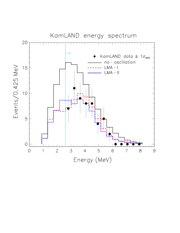
Figure 4: Energy spectra of events in KamLAND for the LMA-I and LMA-II global fit points in Table II, together with the no-oscillation spectrum. The current KamLAND data are superposed above the analysis threshold (2.6 MeV).

The most important task for the next future appears to be the confirmation of one of the two solutions in Fig. 3 through higher statistics and, possibly, lower analysis threshold. Figure 4 shows the absolute KamLAND energy spectra of reactor events predicted at the LMA-I and LMA-II global best-fit points (last two rows of Table I), together with the no-oscillation spectrum, with the current event normalization. The KamLAND data (with statistical errors only) are also superposed above the analysis threshold (2.6 MeV). It can be seen that the main difference between the two oscillated spectra is the position of the spectrum peak, which is roughly aligned with the no-oscillation position for the LMA-II case, while it is shifted at higher energies for the LMA-I case. This feature might be a useful discrimination tool in the next future. From Fig. 4, it appears also that the largest difference between the LMA-I and LMA-II spectra in KamLAND occurs just in the first bin below the current analysis threshold. Therefore, a better understanding of the background below 2.6 MeV will be highly beneficial. In any case, an increase in statistics by a factor of a few appears necessary to disentangle the two oscillated spectra in Fig. 4.

IV $3\nu$ analysis

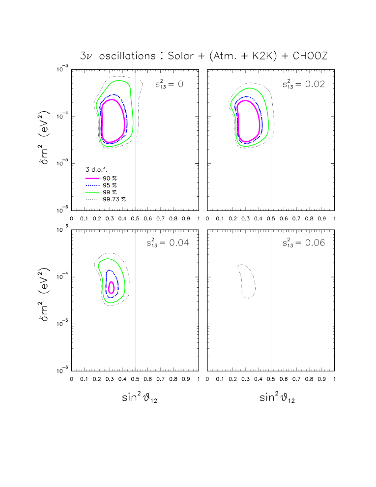
Figure 5: Three-flavor active neutrino oscillations: Global analysis of solar, CHOOZ, and atmospheric+K2K neutrino data, shown as sections of the allowed $(\delta m^{2},\sin^{2}\theta_{12},\sin^{2}\theta_{13})$ parameter space at four representative values of $s^{2}_{13}=\sin^{2}\theta_{13}$. The best fit is reached in the $2\nu$ limit ($s^{2}_{13}=0$), while for increasing $s^{2}_{13}$ the LMA solution shrinks and eventually disappears. The 90, 95, 99, and 99.73% C.L. contours correspond to $\Delta\chi^{2}=6.25$, 7.82, 11.34, and 14.15, respectively (three degrees of freedom). The “atmospheric” mass splitting $\Delta m^{2}$ is minimized away in the fit (see also Las3 ).

The updated $3\nu$ analysis of solar+CHOOZ neutrino data, including the constraints on the large (“atmospheric”) squared mass gap $\Delta m^{2}$ coming from SK atmospheric Shio and K2K accelerator neutrino data K2Ke ; K2Ks , as performed in Las3 , is reported here for the sake of completeness. Figure 5 shows the pre-KamLAND $3\nu$ results Las3 in the parameter space $(\delta m^{2},\sin^{2}\theta_{12},\sin^{2}\theta_{13})$ relevant for the LMA solution, shown through sections at four different values of $s^{2}_{13}=\sin^{2}\theta_{13}$. For later purposes, we only notice that the upper bound on $\delta m^{2}$ becomes stronger for higher $\sin^{2}\theta_{13}$, as a result of the CHOOZ constraints. For a discussion of such $(\delta m^{2},\sin^{2}\theta_{13})$ anti-correlation, and for the pre-KamLAND solutions below the LMA, see Las3 and references therein.

Figure 6 shows the results of our $3\nu$ fit to the KamLAND data, in the same format as in Fig. 5. The allowed $3\nu$ regions appear to get slightly enlarged (especially in the mixing parameter $\theta_{12}$) for increasing values of $\sin^{2}\theta_{13}$, as expected GoKL . In fact, for $\theta_{13}\neq 0$, part of the KamLAND event disappearance is explained by averaged oscillations driven by $\Delta m^{2}$ in the $(\nu_{e},\nu_{3})$ sector, so that the overall oscillation amplitude $\sin^{2}2\theta_{12}$ in the $(\nu_{1},\nu_{2})$ sector is allowed to reach smaller values, and the $\sin^{2}\theta_{12}$ range is correspondingly enlarged GoKL . The absolute $\chi^{2}$ minimum in Fig. 6 is reached for $\theta_{13}\neq 0$, but such preference is not statistically significant, as expected Marf ; indeed, we find a mere $\Delta\chi^{2}=0.4$ increase of the KamLAND $\chi^{2}_{\min}$ value for fixed $\sin^{2}\theta_{13}=0.06$. Concerning the variations of the $(\delta m^{2},\sin^{2}\theta_{12})$ best-fit coordinates for fixed values of $\sin^{2}\theta_{13}$, we find that the $\delta m^{2}$ value is stable (and equal to $7.3\times 10^{-5}$ eV², as in the $2\nu$ case), while $\sin^{2}\theta_{12}$ decreases from 0.335 to 0.225 when increasing $\sin^{2}\theta_{13}$ from 0 to 0.06, in good qualitative agreement with the expectations discussed in GoKL .

However, the additional spread in $\sin^{2}\theta_{12}$ induced by nonzero $\theta_{13}$ currently does not play any relevant role when KamLAND is combined with world neutrino data, for at least two reasons: (1) Pre-KamLAND bounds from solar+terrestrial data currently dominate the constraints on $\sin^{2}\theta_{12}$, as evident from a comparison of Fig. 5 and Fig. 6; (2) The likelihood of genuine $3\nu$-induced effects rapidly decreases with increasing $\theta_{13}$, because of the strong upper bounds on such mixing parameter Las3 . Therefore, we do not expect any significant enlargement of the $\sin^{2}\theta_{12}$ allowed range from the pre- to the post-KamLAND $3\nu$ analysis, despite the presence of such effects in KamLAND alone.

It should be noted that, strictly speaking, Fig. 6 is not exactly a “KamLAND only” analysis, since we have implicitly taken some pieces of information from terrestrial neutrino data. In particular, we have implicitly assumed in Fig. 6 that: (i) the “atmospheric” squared mass splitting $\Delta m^{2}$ is sufficiently high to be unresolved in KamLAND, and (2) the relevant values of $\sin^{2}\theta_{13}$ are limited in the few percent range. It is interesting to study the effect of an explicit combination of such (atmospheric + CHOOZ) information with KamLAND data. The results are given in Fig. 7. This figure show that purely terrestrial neutrino data from atmospheric (SK), accelerator (K2K) and reactor (KamLAND + CHOOZ) neutrino experiments, by themselves, are now able to put both upper and lower bounds on the solar parameters $(\delta m^{2},\sin^{2}\theta_{12})$. As previously noted in the comment to Fig. 5, the CHOOZ upper bound on $\delta m^{2}$ becomes stronger when $\sin^{2}\theta_{13}$ increases. The slight octant asymmetry for $\sin^{2}\theta_{13}>0$ is due to the fact the corresponding $3\nu$ CHOOZ probability is not invariant under the change $\theta_{12}\to\pi/2-\theta_{12}$ for fixed hierarchy QEIP (assumed to be normal in Fig. 6). The octant differences would be swapped by inverting the hierarchy QEIP . In practice, however, such octant asymmetries are numerically irrelevant in the global fit which we now discuss.

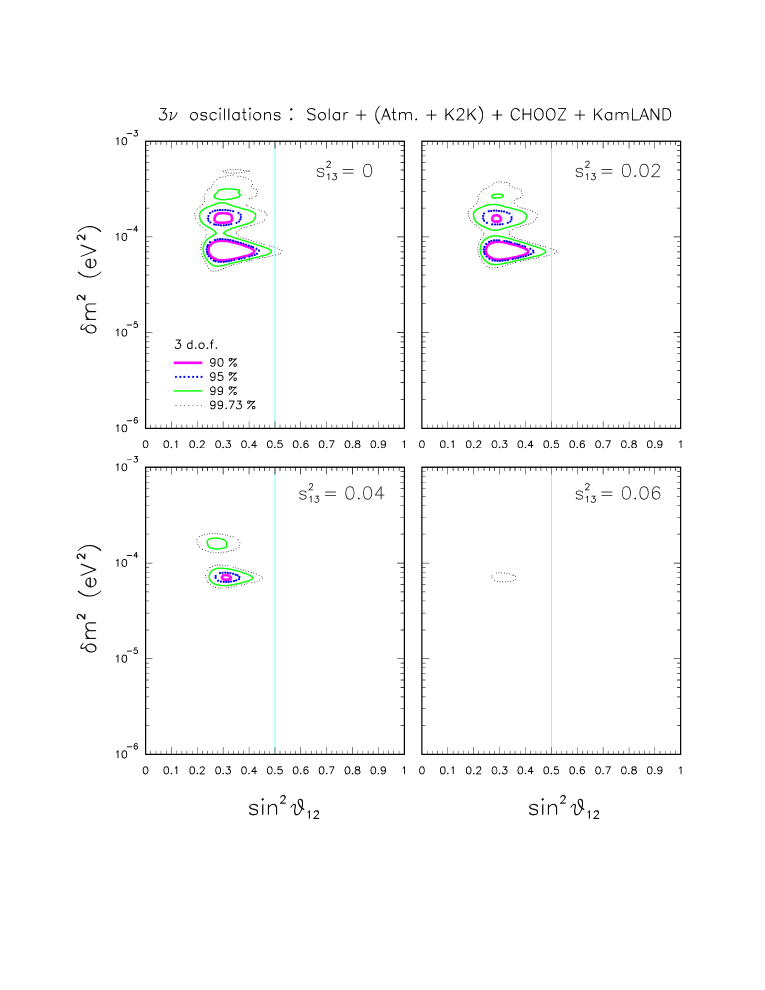
Figure 8: Three-flavor active neutrino oscillations: Global analysis of solar and terrestrial data (including KamLAND), shown in the same format as Fig. 5. With respect to the $2\nu$ case in Fig. 3, the higher $\Delta\chi^{2}$ tolerance induced by an extra degree of freedom (for any chosen C.L.) marginally allows a third “LMA-III” solution at 99% C.L., at about $\delta m^{2}\sim 2.5$–3.2 eV².

Figure 8 shows the final $3\nu$ combination of world (solar+terrestrial) neutrino constraints, including pre-KamLAND data (Fig. 5) and the first KamLAND data (Fig. 6). For $\sin^{2}\theta_{13}=0$ (absolute best fit), we get the same LMA-I and LMA-II solutions reported in Fig. 3 and in Table I, modulo the expected widening induced by one additional degree of freedom in the $\Delta\chi^{2}$’s associated to each C.L. contour. This widening gives, at 99% C.L., marginal allowance for a third solution with $\delta m^{2}\sim 2.5$–$3.2\times 10^{-4}$ eV², which we call LMA-III. All solutions rapidly shrink for increasing $\sin^{2}\theta_{13}$, the LMA-I being the most stable and the last to disappear. The hierarchy is assumed to be normal in Fig. 8; the differences with respect to the inverted hierarchy case (not shown) are completely negligible.

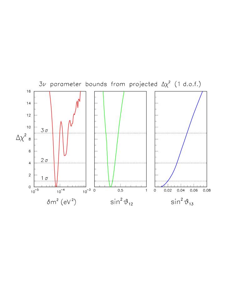
Figure 9: Three-flavor active neutrino oscillations: Projections of the global $(\Delta\chi^{2})$ function onto each of the $(\delta m^{2},\sin^{2}\theta_{12},\sin^{2}\theta_{13})$ parameters. The $n$-sigma bounds on each parameter (the others being unconstrained) correspond to $\Delta\chi^{2}=n^{2}$. In the left panel, the absolute minimum (LMA-I) and the second best fit (LMA-II) are clearly visible. A third shallow minimum (LMA-III) of the $\Delta\chi^{2}(\delta m^{2})$ function is marginally present at $\sim 3.2\sigma$.

Figure 9 represents a compendium of our post-KamLAND $3\nu$ analysis of all data (solar+terrestrial), in terms of the $\Delta\chi^{2}$ function for each of the three variables $(\delta m^{2},\sin^{2}\theta_{12},\sin^{2}\theta_{13})$, the others being projected (minimized) away. This figure should be compared with the pre-KamLAND one in Las3 . The comparison shows that the bounds on $\sin^{2}\theta_{13}$ remain basically unaltered in the post-KamLAND era, while the mixing parameter $\sin^{2}\theta_{12}$ is clearly nailed down around the value $0.3$. The absolute and second best minima (LMA-I and LMA-II) are also evident in the left panel. A third minimum (LMA-III) at higher $\delta m^{2}$ is only marginally allowed.

If we focus on the best-fit (LMA-I) solution, and adapt parabolic functions around the absolute $\chi^{2}$ minima in terms of $\delta m^{2}$ (in linear scale), $\sin^{2}\theta_{13}$, and $\sin^{2}\theta_{13}$, we obtain from the post-KamLAND global analysis the following approximate $\pm 1\sigma$ estimates ($\Delta\chi^{2}\simeq 1$) for the relevant solar $3\nu$ oscillation parameters,

$$\textrm{LMA-I\ }(\sim 1\sigma):\left\{\begin{array}[]{l}\delta m^{2}\simeq(7.3\pm 0.8)\times 10^{-5}\mathrm{\ eV}^{2}\ ,\\ \sin^{2}\theta_{12}\simeq 0.315\pm 0.035\ ,\\ \sin^{2}\theta_{13}\lesssim 0.017\ .\end{array}\right.$$ (2)

The above ranges are meant to show that we are not far from a 10% determination (at $1\sigma$) of both $\delta m^{2}$ and $\sin^{2}\theta_{12}$, but should not be quoted as a “summary” of the current $3\nu$ situation. The technically correct reference summary for our analysis is represented by the $\chi^{2}$ functions of Fig. 9, which include the possibility of a second global best fit (LMA-II), and maybe of a third best fit (LMA-III) in $\delta m^{2}$. In particular, we stress that the LMA-II solution is currently quite acceptable from a statistical point of view, and that the history of the solar neutrino problem teaches us that one should not exclude a priori what may appear as the second best-fit at a particular time.

Similar cautionary remarks also apply to the use of the initial KamLAND data to refine the emerging indications of adiabatic matter effects in the Sun Adia ; Matt through the approach developed in LasA . As stressed in LasA , such analysis will become sufficiently stable and constraining when a single solution (either the LMA-I or the LMA-II) will be (hopefully) clearly selected by KamLAND. In the meantime, further SNO data are also expected to increase our confidence in the occurrence of solar matter effects, see LasA .

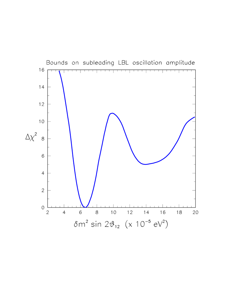
Figure 10: Global bounds on the parameter combination $\delta m^{2}\sin 2\theta_{12}$, governing the amplitude of subleading “solar” neutrino oscillations in long baseline (LBL) experiments. See the text for details.

We conclude our $3\nu$ analysis by observing that, from the point of view of future (very) long baseline (LBL) experiments, the “solar” neutrino parameters $\delta m^{2}$ and $\theta_{12}$ enter the subleading oscillation amplitudes of both the “golden” channel $\nu_{e}\to\nu_{\mu}$ Gold and the “silver” channel $\nu_{e}\to\nu_{\tau}$ Silv only through the combination $\kappa=\delta m^{2}\sin 2\theta_{12}$, up to $O(\kappa^{2})$ terms included Gold ; Silv . Therefore, we think it useful to show in Fig. 10 the global (solar+terrestrial) bounds on this specific combination of parameters (in units of $10^{-5}$ eV² and in linear scale), all other $3\nu$ variables being projected away. The lower and higher minima in Fig. 10 correspond to the LMA-I and LMA-II cases, respectively. By adapting a parabola in the $\pm 2\sigma$ region around each of the two minima, we get the following $1\sigma$ ($\Delta\chi^{2}=1$) estimates for $\kappa=\delta m^{2}\sin 2\theta_{12}$: $\kappa\simeq 6.7\pm 0.7$ (LMA-I) and $\kappa\simeq 14.7\pm 1.7$ (LMA-II), in units of $10^{-5}$ eV². In both cases, $\kappa$ appears to be already constrained with a $\sim 11\%$ accuracy. These approximate estimates—or, better, the accurate bounds in Fig. 10—may prove useful in prospective studies of $\kappa$-dependent subleading oscillation effects in LBL projects.

V Summary and prospects

The KamLAND experiment has clearly selected the LMA region as the solution to the solar neutrino problem, and has further reduced the $(\delta m^{2},\sin^{2}\theta_{12})$ parameter space for active neutrino oscillations. In this work, we have studied such parameter reduction in the the context of $2\nu$ and $3\nu$ oscillations, by using the limited KamLAND experimental information which is publicly available. In the $2\nu$ case, we find that the post-KamLAND LMA solution appears to be basically split into two sub-regions, LMA-I and LMA-II. The LMA-I solution, characterized by $\delta m^{2}\sim 7\times 10^{-5}$ eV² and $\sin^{2}\theta_{12}\sim 0.3$, is preferred by the global fit. The LMA-II solution represents the second best fit, at about twice the value of $\delta m^{2}$ (see Table I). This situation is not significantly changed in the $3\nu$ case, for which we present a global post-KamLAND analysis of solar and terrestrial data in the $(\delta m^{2},\sin^{2}\theta_{12},\sin^{2}\theta_{13})$ parameter space. There are good prospects to separate the LMA-I and LMA-II cases with future, higher-statistics KamLAND data, by looking at the peak of the energy spectrum, and by lowering the current analysis threshold (2.6 MeV) by at least $\sim 0.5$ MeV.

Figure 7: Three-flavor active neutrino oscillations: Global analysis of terrestrial data only (including KamLAND), shown in the same format as Fig. 5. Notice that terrestrial $\nu$ data alone can now put both upper and lower bounds on the solar $\nu$ parameters ($\delta m^{2},\sin^{2}\theta_{12}$). See the text for details.

- (1) SNO Collaboration, Q.R. Ahmad et al., Phys. Rev. Lett. 89, 011301 (2002).
- (2) J.N. Bahcall, Phys. Rev. Lett. 12, 300 (1964); R. Davis, Jr., ibidem, p. 303.
- (3) Homestake Collaboration, B.T. Cleveland, T. Daily, R. Davis Jr., J.R. Distel, K. Lande, C.K. Lee, P.S. Wildenhain, and J. Ullman, Astrophys. J. 496, 505 (1998).
- (4) Kamiokande Collaboration, Y. Fukuda et al., Phys. Rev. Lett. 77, 1683 (1996).
- (5) SAGE Collaboration, J.N. Abdurashitov et al., J. Exp. Theor. Phys. 95, 181 (2002) [Zh. Eksp. Teor. Fiz. 95, 211 (2002)].
- (6) GALLEX Collaboration, W. Hampel et al., Phys. Lett. B 447, 127 (1999).
- (7) T. Kirsten for the GNO Collaboration, in Neutrino 2002, 20th International Conference on Neutrino Physics and Astrophysics (Munich, Germany, 2002). Transparencies available at: neutrino2002.ph.tum.de .
- (8) SK Collaboration, S. Fukuda et al., Phys. Rev. Lett. 86, 5651 (2001); ibidem, 5656 (2001).
- (9) SK Collaboration, S. Fukuda et al., Phys. Lett. B 539, 179 (2002).
- (10) SNO Collaboration, Q.R. Ahmad et al., Phys. Rev. Lett. 87, 071301 (2001).
- (11) SNO Collaboration, Q.R. Ahmad et al., Phys. Rev. Lett. 89, 011302 (2002).
- (12) J.N. Bahcall, Neutrino Astrophysics (Cambridge U. Press, Cambridge, England, 1989).
- (13) J.N. Bahcall, M.H. Pinsonneault, and S. Basu, Astrophys. J. 555, 990 (2001).
- (14) See the website: www.nobel.se .
- (15) KamLAND Collaboration, K. Eguchi et al., Phys. Rev. Lett. 90, 021802 (2003). Additional information available at the sites: hep.stanford.edu/neutrino/KamLAND/KamLAND.html and kamland.lbl.gov .
- (16) B. Pontecorvo, National Research Council of Canada, Division of Atomic Energy, Chalk River Laboratory Report No. P.D. 205, 1946 (unpublished). Available at pontecorvo.jinr.ru .
- (17) L. Alvarez, University of California at Berkeley, Radiation Laboratory Report No. UCRL-328, 1949 (unpublished).
- (18) F. Reines and C.L. Cowan, Jr., Phys. Rev. 92, 830 (1953); ibidem 113, 273 (1959).
- (19) V. Barger, D. Marfatia, K. Whisnant, and B.P. Wood, Phys. Lett. B 537, 179 (2002); A. Bandyopadhyay, S. Choubey, S. Goswami, and D.P. Roy, Phys. Lett. B 540, 14 (2002); J.N. Bahcall, M.C. Gonzalez-Garcia, and C. Peña-Garay, J. High Energy Phys. 7, 54 (2002); A. Strumia, C. Cattadori, N. Ferrari and F. Vissani, Phys. Lett. B 541, 327 (2002); P.C. de Holanda and A.Yu. Smirnov, Phys. Rev. D 66, 113005 (2002); M. Maltoni, T. Schwetz, M.A. Tortola, and J.W.F. Valle, Phys. Rev. D 67, 013011 (2003).
- (20) G.L. Fogli, E. Lisi, A. Marrone, D. Montanino, and A. Palazzo, Phys. Rev. D 66, 053010 (2002).
- (21) G.L. Fogli, G. Lettera, E. Lisi, A. Marrone, A. Palazzo, and A.M. Rotunno, Phys. Rev. D 66, 093008 (2002).
- (22) B. Pontecorvo, Zh. Eksp. Teor. Fiz. 53, 1717 (1968) [Sov. Phys. JETP 26, 984 (1968)].
- (23) Z. Maki, M. Nakagawa, and S. Sakata, Prog. Theor. Phys. 28, 870 (1962).
- (24) See, e.g., the review by A.Yu. Smirnov, in Neutrino 2002 Ki02 , hep-ph/0209131.
- (25) L. Wolfenstein, Phys. Rev. D 17, 2369 (1978); S.P. Mikheev and A.Yu. Smirnov, Yad. Fiz. 42, 1441 (1985) [Sov. J. Nucl. Phys. 42, 913 (1985)].
- (26) V.D. Barger, K. Whisnant, S. Pakvasa, and R.J.N. Phillips, Phys. Rev. D 22, 2718 (1980).
- (27) L. Wolfenstein, in Neutrino ’78, 8th International Conference on Neutrino Physics and Astrophysics (Purdue U., West Lafayette, Indiana, 1978), ed. by E.C. Fowler (Purdue U. Press, 1978), p. C3.
- (28) G.L. Fogli, E. Lisi, A. Palazzo, and A.M. Rotunno, hep-ph/0211414.
- (29) H. Murayama and A. Pierce, Phys. Rev. D 65, 013012 (2002).
- (30) V.D. Barger, D. Marfatia, and B.P. Wood, Phys. Lett. B 498, 53 (2001).
- (31) R. Barbieri and A. Strumia, J. High Energy Phys. 12, 16 (2000).
- (32) A. de Gouvea and C. Peña-Garay, Phys. Rev. D 64, 113011 (2001).
- (33) A. Strumia and F. Vissani, J. High Energy Phys. 11, 48 (2001).
- (34) M.C. Gonzalez-Garcia and C. Peña-Garay, Phys. Lett. B 527, 199 (2002).
- (35) P. Aliani, V. Antonelli, M. Picariello and E. Torrente-Lujan, hep-ph/0207348.
- (36) P.C. de Holanda and A.Yu. Smirnov, in AllS ; see also hep-ph/0211264.
- (37) A. Bandyopadhyay, S. Choubey, R. Gandhi, S. Goswami, and D.P. Roy, hep-ph/0211266.
- (38) CHOOZ Collaboration, M. Apollonio et al., Phys. Lett. B 466, 415 (1999); M. Apollonio et al., hep-ex/0301017, to appear in Eur. Phys. J. C.
- (39) M. Shiozawa for the SK Collaboration, in Neutrino 2002 Ki02 .
- (40) K. Nishikawa for the K2K Collaboration, in Neutrino 2002 Ki02 .
- (41) K2K Collaboration, M.H. Ahn et al., Phys. Rev. Lett. 90, 041801 (2003).
- (42) Review of Particle Physics, K. Hagiwara et al., Phys. Rev. D 66, 010001 (2002).
- (43) L.M. Krauss, S.L. Glashow, and D.N. Schramm, Nature 310, 191 (1984); R.S. Raghavan, S. Schonert, S. Enomoto, J. Shirai, F. Suekane, and A. Suzuki, Phys. Rev. Lett. 80, 635 (1998); M. Kobayashi and Y. Fukao, Geophys. Res. Lett. 18, 633 (1991); C.G. Rothschild, M.C. Chen, and F.P. Calaprice, Ann. Geophys. 25 (1998), 1083.
- (44) P. Huber, M. Lindner, and W. Winter, Nucl. Phys. B 645, 3 (2002).
- (45) E. Lisi, A. Marrone, and D. Montanino, work in progress.
- (46) S.M. Bilenky, D. Nicolo, and S.T. Petcov, Phys. Lett. B 538, 77 (2002); M.C. Gonzalez-Garcia and M. Maltoni, hep-ph/0202218.
- (47) G.L. Fogli, E. Lisi, and A. Palazzo, Phys. Rev. D 65, 073019 (2002).
- (48) M. Freund, Phys. Rev. D 64, 053003 (2001); A. Cervera et al., Nucl. Phys. B 579, 731 (2001).
- (49) A. Donini, D. Meloni, and P. Migliozzi, Nucl. Phys. B 646, 321 (2002); V. Barger, D. Marfatia, and K. Whisnant, Phys. Rev. D 65, 073023 (2002).