TUM-HEP-542/04

Series expansions for three-flavor neutrino oscillation
probabilities in matter

Evgeny K. Akhmedov, Robert Johansson, Manfred Lindner,
Tommy Ohlsson, and Thomas Schwetz 

Instituto de Física Corpuscular – C.S.I.C./Universitat de València,

Edificio Institutos de Paterna, Apt 22085, 46071 Valencia, Spain

^,Division of Mathematical Physics, Department of Physics,

Royal Institute of Technology (KTH) – AlbaNova University Center,

Roslagstullsbacken 11, 106 91 Stockholm, Sweden

^,Theoretische Physik, Physik-Department,

Technische Universität München (TUM),

James-Franck-Straße, 85748 Garching bei München, Germany

Abstract

We present a number of complete sets of series expansion formulas for neutrino oscillation probabilities in matter of constant density for three flavors. In particular, we study expansions in the mass hierarchy parameter $\alpha\equiv\Delta m_{21}^{2}/\Delta m_{31}^{2}$ and mixing parameter $s_{13}\equiv\sin\theta_{13}$ up to second order and expansions only in $\alpha$ and only in $s_{13}$ up to first order. For each type of expansion we also present the corresponding formulas for neutrino oscillations in vacuum. We perform a detailed analysis of the accuracy of the different sets of series expansion formulas and investigate which type of expansion is most accurate in different regions of the parameter space spanned by the neutrino energy $E$, the baseline length $L$, and the expansion parameters $\alpha$ and $s_{13}$. We also present the formulas for series expansions in $\alpha$ and in $s_{13}$ up to first order for the case of arbitrary matter density profiles. Furthermore, it is shown that in general all the 18 neutrino and antineutrino oscillation probabilities can be expressed through just two independent probabilities.

1 Introduction

The discovery of neutrino oscillations in atmospheric, solar, and reactor neutrino experiments has turned neutrino physics into one of the most exciting and active fields of particle physics. By now, a significant amount of information on neutrino properties has been obtained. The results of the atmospheric neutrino experiments [1, 2, 3] and the K2K accelerator neutrino experiment [4] have allowed the determination of the fundamental neutrino parameters $\Delta m_{31}^{2}$ and $\theta_{23}$ to an accuracy of about 30% and 15%, respectively, while the solar neutrino experiments [5] and the KamLAND reactor neutrino experiment [6] have measured the parameters $\Delta m_{21}^{2}$ and $\theta_{12}$ to an accuracy of about 15%. In fact, this means that neutrino physics is now entering an era of precision measurements of the neutrino oscillation parameters. Future experiments with superbeams and neutrino factories will determine the “atmospheric” and “solar” neutrino oscillation parameters to an accuracy of the order of 1%. They are also expected to measure the elusive leptonic mixing angle $\theta_{13}$ for which at present only an upper limit exists [7], or to put a more stringent limit on this angle, as well as to clarify the issues of the neutrino mass hierarchy and possibly of leptonic CP violation. Important information on neutrino oscillation parameters can also be obtained from the future atmospheric, solar, reactor, and supernova neutrino experiments.

Increasing accuracy and reach of the present and especially of forthcoming experiments put forward new and more challenging demands to the theoretical description of neutrino oscillations. In order to be able to determine the fundamental neutrino parameters from the data with high precision, one needs, among other things, very accurate theoretical expressions for the probabilities of neutrino oscillations in matter and in vacuum. While these probabilities can, in principle, be calculated numerically with any requisite accuracy, it is highly desirable to have also analytic expressions for them. Such analytic expressions would reveal the basic dependence of the neutrino oscillation probabilities on the fundamental neutrino parameters and on the characteristics of the experiment and thus facilitate the choice of the experimental setup as well as the analysis of the data. They would also help to understand the physics underlying various flavor transitions and to resolve the parameter degeneracies and other ambiguities, such as fundamental versus matter-induced CP violation.

The purpose of this paper is to present a collection of approximate analytic formulas for the neutrino oscillation probabilities. We derive a number of complete sets of series expansion formulas for the three-flavor neutrino oscillation probabilities in matter and in vacuum. The probabilities are expanded in the mass hierarchy parameter $\alpha\equiv\Delta m_{21}^{2}/\Delta m_{31}^{2}$, the mixing parameter $s_{13}\equiv\sin\theta_{13}$, or in both of them. We also study in detail the accuracy of the obtained expressions in different regions of the parameter space and identify the “best choice” in each case of interest.

Before proceeding to present our results, we give here a brief overview of the previous work on the subject. Analytic formulas for three-flavor neutrino oscillation probabilities have been derived in a number of papers. Exact formulas for the neutrino oscillation probabilities in vacuum can be found, e.g., in Ref. [8]. Exact expressions can also be obtained in the case of three-flavor neutrino oscillations in matter of constant density [9, 10, 11, 12, 13, 14, 15, 16]. However, the corresponding formulas are rather complicated and not easily tractable. This also applies to the exact analytic three-flavor formulas obtained for some special cases of non-uniform matter density: linear matter density [17] and exponentially varying matter density [18].

Approximate analytic formulas for three-flavor neutrino oscillation probabilities in matter have been derived in a number of papers, see e.g., Refs. [19, 20, 21, 22, 23, 24]. In Refs. [19, 20], the Mikheyev–Smirnov–Wolfenstein (MSW) resonances [25] in matter of varying density were studied assuming large separation and independence of the high-density and low-density resonances. In Refs. [20, 21, 23], the adiabatic approximation was used to derive three-flavor neutrino oscillation probabilities in matter of varying density, whereas in Ref. [24], the Magnus expansion for the time evolution operator was used, which is equivalent to the anti-adiabatic approximation.

In a number of papers an approach similar to ours was adopted, i.e., the neutrino oscillation probabilities were expanded in the small parameters $\alpha$, $s_{13}$, or in both of them. In Ref. [26], exact analytic expressions for three-flavor neutrino oscillation probabilities in matter with an arbitrary density profile were obtained in the limit $\alpha\to 0$ by reducing the problem to an effective two-flavor one. In Ref. [27], a similar approach was employed to obtain the neutrino oscillation probabilities in matter of arbitrarily varying density in the limit $\theta_{13}\to 0$, whereas in Refs. [28, 29], expressions up to first order in $s_{13}$ were derived. For the case of matter of constant density, the limit $\alpha\to 0$ was considered in Ref. [30]. Expansions up to first order in $\alpha$ were carried out in Refs. [31, 32]. In Refs. [33, 34], both the solar mass squared difference $\Delta m_{21}^{2}$ and matter effects were treated as perturbations and the transition probabilities up to first order in them were derived. Expansions in both $\alpha$ and $s_{13}$ were used in Refs. [35, 36, 37, 38]. We note that the neutrino oscillation probabilities derived in most of the above-mentioned papers either did not constitute a complete set (i.e., a set of probabilities from which the probabilities in all channels can be obtained), or contained expressions from which some terms were missing, especially in the case of the probabilities $P(\nu_{\mu}\to\nu_{\mu})$ and $P(\nu_{\mu}\to\nu_{\tau})$. Thus, to the best of our knowledge, our study is the first one in which, for the case of matter of constant density, complete and consistent expansions in $\alpha$ and $s_{13}$ to second order and expansions only in $\alpha$ and only in $s_{13}$ up to first order are performed.

The paper is organized as follows. In Sec. 2 we set the general formalism and notation, discuss some general relations satisfied by the oscillation probabilities, and show that all the 18 neutrino and antineutrino oscillation probabilities can be expressed through just two independent probabilities. In Sec. 3 we present a series expansion of the neutrino oscillation probabilities up to second order in both $\alpha$ and $s_{13}$ (the so-called “double expansion”), whereas in Secs. 4 and 5 we consider the probabilities expanded up to first order in $\alpha$ and $s_{13}$, respectively (“single expansions”). In all three cases, we give the probabilities for matter of constant density (Secs. 3.1, 4.1, and 5.1) and in vacuum (Secs. 3.2, 4.2, and 5.2). We also compare our formulas with the corresponding expressions existing in the literature (when available), pointing out agreements and disagreements. In Sec. 6, we discuss the qualitative behavior of the neutrino oscillation probabilities, the relevance of matter effects, and give a detailed evaluation of the accuracy of the various formulas. Furthermore, we comment on the application of our probability formulas to neutrino oscillation experiments. We summarize our results in Sec. 7. Finally, several methods that have been used to derive the formulas are presented in the appendices. In Appendix A, we describe the perturbative diagonalization of the effective Hamiltonian of the neutrino system in the case of matter of constant density, while in Appendix B, the details of the perturbative expansion of the neutrino evolution equation in the case of arbitrary matter density profiles are given.

2 General formalism and notation

We consider three-flavor neutrino oscillations and adopt the standard parameterization of the leptonic mixing matrix $U$ [39]:

$$U =O_{23}U_{\delta}O_{13}U^{\dagger}_{\delta}O_{12}$$

$$=\left(\begin{matrix}c_{12}c_{13}&s_{12}c_{13}&s_{13}{\rm e}^{-{\rm i}\delta_{\rm CP}}\\ -s_{12}c_{23}-c_{12}s_{13}s_{23}{\rm e}^{{\rm i}\delta_{\rm CP}}&c_{12}c_{23}-s_{12}s_{13}s_{23}{\rm e}^{{\rm i}\delta_{\rm CP}}&c_{13}s_{23}\\ s_{12}s_{23}-c_{12}s_{13}c_{23}{\rm e}^{{\rm i}\delta_{\rm CP}}&-c_{12}s_{23}-s_{12}s_{13}c_{23}{\rm e}^{{\rm i}\delta_{\rm CP}}&c_{13}c_{23}\end{matrix}\right)\,.$$ (1)

Here $O_{ij}$ is the orthogonal rotation matrix in the $ij$-plane which depends on the mixing angle $\theta_{ij}$, $U_{\delta}=\mathrm{diag}(1,1,{\rm e}^{{\rm i}\delta_{\rm CP}})$, $\delta_{\rm CP}$ being the Dirac-type CP-violating phase, $s_{ij}\equiv\sin\theta_{ij}$ and $c_{ij}\equiv\cos\theta_{ij}$. In the three-flavor case there are also, in general, two Majorana-type CP-violating phases; however, these phases do not affect neutrino oscillations, and therefore will not be considered here. Without loss of generality, one can assume all the mixing angles to lie in the first quadrant (i.e., between 0 and $\pi/2$), while the CP-violating phase $\delta_{\rm CP}$ is allowed to lie in the interval $[0,\,2\pi]$.

Let us denote by $P_{\alpha\beta}\equiv P(\nu_{\alpha}\to\nu_{\beta})$ the probability of transition from a neutrino flavor $\alpha$ to a neutrino flavor $\beta$, and similarly for antineutrino flavors, i.e., $P_{\bar{\alpha}\bar{\beta}}\equiv P(\bar{\nu}_{\alpha}\to\bar{\nu}_{\beta})$. In general, the three-flavor neutrino oscillation probabilities in matter $P_{\alpha\beta}$ depend on eight parameters and one function:

$$P_{\alpha\beta}=P_{\alpha\beta}(\Delta m_{21}^{2},\Delta m_{31}^{2},\theta_{12},\theta_{13},\theta_{23},\delta_{\rm CP};E,L,V(x)),\quad\alpha,\beta=e,\mu,\tau\,.$$ (2)

Here $\Delta m_{ij}^{2}\equiv m^{2}_{i}-m^{2}_{j}$ are the neutrino mass squared differences, $E$ is the neutrino energy, $L$ is the baseline length, and $V(x)$ is the matter-induced effective potential, $x\in[0,L]$ being the coordinate along the neutrino path. The neutrino mass squared differences, the leptonic mixing angles, and the CP-violating phase are fundamental parameters and thus experiment-independent, whereas the neutrino energy, the baseline length, and the matter-induced effective potential vary from experiment to experiment. The present best-fit values and 3$\sigma$ allowed ranges of the fundamental neutrino parameters found in a recent global fit of the neutrino oscillation data [40] are summarized in Table 1. Unless otherwise stated, all calculations in the present paper are performed for the following values of the neutrino parameters: $\Delta m_{21}^{2}=7\cdot 10^{-5}\,{\rm eV}^{2}$, $\theta_{12}=33^{\circ}$, and $\theta_{23}=45^{\circ}$. For the atmospheric mass squared difference $\Delta m_{31}^{2}$ we adopt the current best-fit value given by the Super-Kamiokande Collaboration, $|\Delta m_{31}^{2}|=2\cdot 10^{-3}\,{\rm eV}^{2}$ [2], which is slightly smaller than the value given in Table 1. The sign of $\Delta m_{31}^{2}$ is related to the neutrino mass hierarchy: for the normal (inverted) hierarchy one has $\Delta m_{31}^{2}>0$ ($\Delta m_{31}^{2}<0$). For the leptonic mixing angle $\theta_{13}$ we allow values below the 90% C.L. upper bound found in the global fit of the neutrino oscillation data [40] for $|\Delta m_{31}^{2}|$ fixed at $2\cdot 10^{-3}\,{\rm eV}^{2}$:

$$\theta_{13}\lesssim 10.8^{\circ}\,,\quad\mbox{or}\quad s_{13}\equiv\sin\theta_{13}\lesssim 0.19\,,\quad\mbox{or}\quad\sin^{2}2\theta_{13}\lesssim 0.14\,.$$ (3)

For the CP violation phase $\delta_{\mathrm{CP}}$ we allow values between $0$ and $2\pi$.

Parameter	Best-fit value	Range ($3\sigma$)
$\Delta m_{21}^{2}$	$6.9\cdot 10^{-5}\,{\rm eV}^{2}$	$(5.4\div 9.5)\cdot 10^{-5}\,{\rm eV}^{2}$
$|\Delta m_{31}^{2}|$	$2.6\cdot 10^{-3}\,{\rm eV}^{2}$	$(1.5\div 3.7)\cdot 10^{-3}\,{\rm eV}^{2}$
$\theta_{12}$	$33.2^{\circ}$	$28.6^{\circ}\div 38.6^{\circ}$
$\theta_{13}$	$4.4^{\circ}$	$0\div 13.4^{\circ}$
$\theta_{23}$	$46.1^{\circ}$	$33.8^{\circ}\div 58.1^{\circ}$
$\delta_{\rm CP}$	-	$0\div 2\pi$

Table 1: Present best-fit values and $3\sigma$ allowed ranges of the fundamental neutrino parameters from a three-flavor fit to global neutrino oscillation data [40].

Inspecting the values of the fundamental neutrino parameters in Table 1, one can identify two natural candidates for small expansion parameters of the neutrino oscillation probabilities. These are the small leptonic mixing angle $\theta_{13}$ (or, equivalently, $s_{13}$) and the mass hierarchy parameter

$$\alpha\equiv\frac{\Delta m_{21}^{2}}{\Delta m_{31}^{2}}\simeq 0.026\,,\quad(0.018)~{}0.021\lesssim\alpha\lesssim 0.036~{}(0.053)\quad\mbox{at 90\% C.L. ($3\sigma$)\,,}$$ (4)

where we have taken the current best-fit value and allowed ranges from Ref. [40]. In the following, we will derive a number of formulas for series expansions of the neutrino oscillation probabilities in these small quantities. Comparing Eqs. (3) and (4), one realizes that current data constrain the parameter $\alpha$ to a relatively narrow range, while $s_{13}$ is only bounded from above and might be significantly larger or smaller than $\alpha$. The relative size of these two expansion parameters will be important for the validity of a given type of expansion.

In order to find the neutrino oscillation probabilities for a given experimental setup, one has, in general, to solve the Schrödinger equation for the neutrino vector of state in the flavor basis $|\nu(t)\rangle=(\begin{matrix}\nu_{e}(t)&\nu_{\mu}(t)&\nu_{\tau}(t)\end{matrix})^{T}$:

$${\rm i}\frac{{\rm d}}{{\rm d}t}|\nu(t)\rangle=H|\nu(t)\rangle$$ (5)

with the effective Hamiltonian

$$H\simeq\frac{1}{2E}U\,\mathrm{diag}(0,\Delta m_{21}^{2},\Delta m_{31}^{2})U^{\dagger}+\mathrm{diag}(V,0,0)\,.$$ (6)

Here $V$ is the charged-current contribution to the matter-induced effective potential of $\nu_{e}$ [25]. We have disregarded the neutral-current contributions to the neutrino potentials in matter, since they are the same for $\nu_{e}$, $\nu_{\mu}$, and $\nu_{\tau}$  and so do not affect neutrino oscillations. Note that Eq. (6) holds for neutrinos, whereas for antineutrinos one has to perform the replacements

$$U\to U^{*}\>,\quad V\to-V\,.$$ (7)

The potential $V(x)$ is given in convenient units by

$$V(x)\simeq 7.56\times 10^{-14}\left(\frac{\rho(x)}{\mathrm{g/cm^{3}}}\right)Y_{e}(x)\;\;\mathrm{eV}\,,$$ (8)

where $\rho(x)$ is the matter density along the neutrino path and $Y_{e}(x)$ is the number of electrons per nucleon. For the matter of the Earth one has, to a very good accuracy, $Y_{e}\simeq 0.5$.

For many practical applications (such as long-baseline accelerator experiments, as well as oscillations of atmospheric, solar, and supernova neutrinos inside the Earth when they do not cross the Earth’s core) it is a very good approximation to assume that the matter density along the neutrino trajectory is constant (see, e.g., Refs. [42, 43, 44]). Typical values for the matter density are $\rho_{\rm crust}\simeq 3\,{\rm g/cm^{3}}$ in the Earth’s crust and $\rho_{\rm mantle}\simeq 4.5\,{\rm g/cm^{3}}$ in its mantle. In situations where the neutrinos also cross the Earth’s core or for strongly varying matter density profiles like those inside the Sun or supernovae, the constant matter density approximation is not valid.

The neutrino oscillation probabilities can be found as $P_{\alpha\beta}=|S_{\beta\alpha}(t,t_{0})|^{2}$, where $S(t,t_{0})$ is the evolution matrix such that

$$|\nu(t)\rangle=S(t,t_{0})|\nu(t_{0})\rangle\,,\qquad\qquad S(t_{0},t_{0})=\mathbbm{1}\,.$$ (9)

Note that $S(t,t_{0})$ satisfies the same Schrödinger equation, Eq. (5), as $|\nu(t)\rangle$. In the case of matter of constant density, the evolution matrix can be obtained by diagonalizing the Hamiltonian in Eq. (6) according to $H=U^{\prime}\hat{H}U^{\prime\dagger}$, where $U^{\prime}$ is the leptonic mixing matrix in matter and $\hat{H}=\mathrm{diag}(E_{1},E_{2},E_{3})$. The evolution matrix is then given by

$$S_{\beta\alpha}(t,t_{0})=\sum_{i=1}^{3}(U^{\prime}_{\alpha i})^{*}U^{\prime}_{\beta i}{\rm e}^{-{\rm i}E_{i}L}\,,\qquad\alpha,\beta=e,\mu,\tau\,,$$ (10)

where we have identified $L\equiv t-t_{0}$.

Before presenting our results for the neutrino oscillation probabilities, we discuss some of their general properties as well as relations between them. First, we note that Eq. (7) implies that one can relate the oscillation probabilities for antineutrinos to those for neutrinos by

$$P_{\bar{\alpha}\bar{\beta}}=P_{\alpha\beta}(\delta_{\rm CP}\to-\delta_{\rm CP},\,V\to-V)\,,\qquad\alpha,\beta=e,\mu,\tau\,.$$ (11)

Second, in general, i.e., both in vacuum and in matter with an arbitrary density profile, it follows from the unitarity of $S(t,t_{0})$ (conservation of probability) that

$$\sum_{\alpha}P_{\alpha\beta}=\sum_{\beta}P_{\alpha\beta}=1\,,\qquad\alpha,\beta=e,\mu,\tau\,.$$ (12)

These relations imply that five out of the nine neutrino oscillation probabilities can be expressed in terms of the other four [45].

Besides these general properties, there exists an additional symmetry due to the specific parameterization of the mixing matrix given in Eq. (1) and the fact that the rotation matrix $O_{23}$ commutes with the matter potential term of the Hamiltonian in Eq. (6). It is easy to show that the evolution matrix can be written as

$$S(t,t_{0})=O_{23}S^{\prime}(t,t_{0})O_{23}^{T}$$ (13)

where $S^{\prime}(t,t_{0})$ does not depend on $\theta_{23}$. This can be used to prove some useful relations between the probabilities. Let us denote 

$$\tilde{P}_{\alpha\beta}\equiv P_{\alpha\beta}(s_{23}^{2}\leftrightarrow c_{23}^{2}\,,\;\sin 2\theta_{23}\to-\sin 2\theta_{23})\,,\qquad\alpha,\beta=e,\mu,\tau\,.$$ (14)

Using Eqs. (13) and (14), one can readily show that

$$P_{e\tau}=\tilde{P}_{e\mu}\,,\qquad\quad P_{\tau\mu}=\tilde{P}_{\mu\tau}\,,\qquad\quad P_{\tau\tau}=\tilde{P}_{\mu\mu}\,,$$ (15)

while $P_{ee}$ turns out to be independent of $\theta_{23}$.

Out of the three conditions in Eq. (15), only two are independent, as each of them can be derived from the other two and the unitarity conditions (12). Hence, the number of independent neutrino oscillation probabilities is reduced to two. Thus, we come to the important conclusion that all the nine neutrino oscillation probabilities can be expressed through just two independent probabilities provided that their dependence on the mixing angle $\theta_{23}$ is known. However, the choice of these independent probabilities is restricted: they should not include $P_{ee}$, which is independent of $\theta_{23}$; nor should they be a pair of the probabilities, which are T-reverse of each other, or go into each other (or T-reverse of each other) under the transformation $s_{23}^{2}\leftrightarrow c_{23}^{2}\,,\;\sin 2\theta_{23}\to-\sin 2\theta_{23}$.

One possible choice, and the one that we will use, is $P_{e\mu}$ and $P_{\mu\tau}$. For completeness, we give here the expressions for all the other neutrino oscillation probabilities in terms of these two. Using Eqs. (12) and (15), one easily finds

$$P_{ee} =1-(P_{e\mu}+\tilde{P}_{e\mu})\,,$$ (16)

$$P_{e\tau} =\tilde{P}_{e\mu}\,,$$ (17)

$$P_{\mu e} =P_{e\mu}-P_{\mu\tau}+\tilde{P}_{\mu\tau}\,,$$ (18)

$$P_{\mu\mu} =1-P_{e\mu}-\tilde{P}_{\mu\tau}\,,$$ (19)

$$P_{\tau e} =\tilde{P}_{e\mu}+P_{\mu\tau}-\tilde{P}_{\mu\tau}\,,$$ (20)

$$P_{\tau\mu} =\tilde{P}_{\mu\tau}\,,$$ (21)

$$P_{\tau\tau} =1-(\tilde{P}_{e\mu}+P_{\mu\tau})\,.$$ (22)

In addition to the above relations, one can study the transformations of the neutrino oscillation probabilities under the time reversal $P_{\alpha\beta}\to P_{\beta\alpha}$. It can be shown [28] that in matter with an arbitrary density profile

$$P_{\beta\alpha}=P_{\alpha\beta}(\delta_{\rm CP}\to-\delta_{\rm CP},\,V(x)\to V_{\rm rev}(x))\,,\qquad\alpha,\beta=e,\mu,\tau\,,$$ (23)

where $V_{\rm rev}(x)$ is the “reverse” potential, which corresponds to the interchanged positions of the neutrino source and the detector. In the case of symmetric matter density profiles (including matter of constant density), $V_{\rm rev}(x)=V(x)$, and Eq. (23) simplifies to

$$P_{\beta\alpha}=P_{\alpha\beta}(\delta_{\rm CP}\to-\delta_{\rm CP})\,,\qquad\alpha,\beta=e,\mu,\tau\,.$$ (24)

While Eq. (24) does not further reduce the number of independent probabilities, it yields relations which can be useful for cross-checking the formulas for $P_{\alpha\beta}$ in the case of matter with symmetric density profiles.

By applying the rule given in Eq. (11), one can obtain from Eqs. (16)–(22) the corresponding probabilities for the antineutrino oscillations. Thus, the expressions for all 18 probabilities of neutrino and antineutrino oscillations can be found from the formulas for just two independent neutrino oscillation probabilities, which, as was already mentioned, we choose to be $P_{e\mu}$ and $P_{\mu\tau}$. In order to be more explicit, we will in some cases also give formulas for additional neutrino oscillation channels.

In the following Secs. 3, 4, and 5, we give our results for the various series expansions of the neutrino oscillation probabilities. We will adopt the following abbreviations:

$$\Delta \equiv\frac{\Delta m^{2}_{31}L}{4E}\,,$$ (25)

$$A \equiv\frac{2EV}{\Delta m^{2}_{31}}=\frac{VL}{2\Delta}\,.$$ (26)

3 Series expansion up to second order in $\alpha$ and $s_{13}$

3.1 Matter of constant density

In this section, we present the series expansion formulas for three-flavor neutrino oscillation probabilities in matter of constant density up to second order in both $\alpha$ and $s_{13}$. The probabilities are calculated by diagonalizing the Hamiltonian (6) up to second order in these parameters, as described in Appendix A.1. We find for the eigenvalues of the Hamiltonian

$$E_{1} \simeq\frac{\Delta m_{31}^{2}}{2E}\,\left(A+\alpha\,s_{12}^{2}+s_{13}^{2}\,\frac{A}{A-1}+\alpha^{2}\,\frac{\sin^{2}2\theta_{12}}{4A}\right)\,,$$ (27)

$$E_{2} \simeq\frac{\Delta m_{31}^{2}}{2E}\,\left(\alpha\,c_{12}^{2}-\alpha^{2}\,\frac{\sin^{2}2\theta_{12}}{4A}\right)\,,$$ (28)

$$E_{3} \simeq\frac{\Delta m_{31}^{2}}{2E}\,\left(1-s_{13}^{2}\,\frac{A}{A-1}\right)\,.$$ (29)

Calculating the mixing matrix in matter $U^{\prime}$ as described in Appendix A.1 and using Eq. (10) for the evolution matrix $S$, it is straightforward (although somewhat tedious) to derive the following expressions for the neutrino oscillation probabilities:

$$P_{ee} =1-\alpha^{2}\,\sin^{2}2\theta_{12}\,\frac{\sin^{2}A\Delta}{A^{2}}-4\,s_{13}^{2}\,\frac{\sin^{2}(A-1)\Delta}{(A-1)^{2}}\,,$$ (30)

$$P_{e\mu} =\alpha^{2}\,\sin^{2}2\theta_{12}\,c_{23}^{2}\frac{\sin^{2}A\Delta}{A^{2}}+4\,s_{13}^{2}\,s_{23}^{2}\frac{\sin^{2}(A-1)\Delta}{(A-1)^{2}}$$

$$+2\,\alpha\,s_{13}\,\sin 2\theta_{12}\,\sin 2\theta_{23}\cos(\Delta-\delta_{\rm CP})\,\frac{\sin A\Delta}{A}\,\frac{\sin(A-1)\Delta}{A-1}\,,$$ (31)

$$P_{e\tau} =\alpha^{2}\,\sin^{2}2\theta_{12}\,s_{23}^{2}\frac{\sin^{2}A\Delta}{A^{2}}+4\,s_{13}^{2}\,c_{23}^{2}\frac{\sin^{2}(A-1)\Delta}{(A-1)^{2}}$$

$$-2\,\alpha\,s_{13}\,\sin 2\theta_{12}\,\sin 2\theta_{23}\cos(\Delta-\delta_{\rm CP})\,\frac{\sin A\Delta}{A}\,\frac{\sin(A-1)\Delta}{A-1}\,,$$ (32)

$$P_{\mu\mu} =1-\sin^{2}2\theta_{23}\,\sin^{2}\Delta+\alpha\,c_{12}^{2}\,\sin^{2}2\theta_{23}\,\Delta\,\sin 2\Delta$$

$$-\alpha^{2}\,\sin^{2}2\theta_{12}\,c_{23}^{2}\,\frac{\sin^{2}A\Delta}{A^{2}}-\alpha^{2}\,c_{12}^{4}\,\sin^{2}2\theta_{23}\,\Delta^{2}\,\cos 2\Delta$$

$$+\frac{1}{2A}\,\alpha^{2}\,\sin^{2}2\theta_{12}\,\sin^{2}2\theta_{23}\left(\sin\Delta\,\frac{\sin A\Delta}{A}\,\cos(A-1)\Delta-\frac{\Delta}{2}\,\sin 2\Delta\right)$$

$$-4\,s_{13}^{2}\,s_{23}^{2}\frac{\sin^{2}(A-1)\Delta}{(A-1)^{2}}$$

$$-\frac{2}{A-1}\,s_{13}^{2}\,\sin^{2}2\theta_{23}\left(\sin\Delta\,\cos A\Delta\,\frac{\sin(A-1)\Delta}{A-1}-\frac{A}{2}\Delta\,\sin 2\Delta\right)$$

$$-2\,\alpha\,s_{13}\,\sin 2\theta_{12}\,\sin 2\theta_{23}\,\cos\delta_{\rm CP}\,\cos\Delta\,\frac{\sin A\Delta}{A}\,\frac{\sin(A-1)\Delta}{A-1}$$

$$+\frac{2}{A-1}\,\alpha\,s_{13}\,\sin 2\theta_{12}\,\sin 2\theta_{23}\,\cos 2\theta_{23}\,\cos\delta_{\rm CP}\,\sin\Delta\left(A\sin\Delta-\frac{\sin A\Delta}{A}\,\cos(A-1)\Delta\right)\,,$$ (33)

$$P_{\mu\tau} =\sin^{2}2\theta_{23}\,\sin^{2}\Delta-\alpha\,c_{12}^{2}\,\sin^{2}2\theta_{23}\,\Delta\,\sin 2\Delta+\alpha^{2}\,c_{12}^{4}\,\sin^{2}2\theta_{23}\,\Delta^{2}\,\cos 2\Delta$$

$$-\frac{1}{2A}\,\alpha^{2}\,\sin^{2}2\theta_{12}\,\sin^{2}2\theta_{23}\left(\sin\Delta\,\frac{\sin A\Delta}{A}\,\cos(A-1)\Delta-\frac{\Delta}{2}\,\sin 2\Delta\right)$$

$$+\frac{2}{A-1}\,s_{13}^{2}\,\sin^{2}2\theta_{23}\left(\sin\Delta\,\cos A\Delta\,\frac{\sin(A-1)\Delta}{A-1}-\frac{A}{2}\Delta\,\sin 2\Delta\right)$$

$$+2\,\alpha\,s_{13}\,\sin 2\theta_{12}\,\sin 2\theta_{23}\,\sin\delta_{\rm CP}\,\sin\Delta\,\frac{\sin A\Delta}{A}\,\frac{\sin(A-1)\Delta}{A-1}$$

$$-\frac{2}{A-1}\,\alpha\,s_{13}\,\sin 2\theta_{12}\,\sin 2\theta_{23}\,\cos 2\theta_{23}\,\cos\delta_{\rm CP}\,\sin\Delta\left(A\sin\Delta-\frac{\sin A\Delta}{A}\,\cos(A-1)\Delta\right)\,.$$ (34)

Formally, our calculations are based upon the approximations $\alpha,s_{13}\ll 1$ and no explicit assumptions about the values of $L/E$ are made. However, we remark that the series expansion formulas (30)–(34) are no longer valid as soon as $\alpha\Delta=\Delta m^{2}_{21}L/(4E)$ becomes of order unity, i.e., when the oscillatory behavior due to the “solar” mass squared difference $\Delta m_{21}^{2}$ becomes relevant. This can happen for very long baselines and/or very low energies. See also Sec. 6 for a detailed discussion of the accuracy of these formulas.

From Eqs. (27)–(29) one can see that in vacuum ($A=0$) and at the atmospheric resonance ($A=1$) the expressions for the eigenvalues are divergent, and one would expect the expansion to break down. In these cases, two out of the three eigenvalues of the unperturbed Hamiltonian are degenerate and, strictly speaking, the degenerate perturbation theory rather than the ordinary one should be employed. However, it turns out that, though the eigenvalues (27)–(29) are divergent, the neutrino oscillation probabilities are finite in the limits $A\to 0$ and $A\to 1$. The reason for this interesting behavior is a cancellation of divergences between the eigenvalues and the matrix elements of the leptonic mixing matrix in the calculation of the evolution matrix according to Eq. (10). In particular, in the limit $A\to 0$, the correct vacuum neutrino oscillation probabilities are obtained.

We shall now compare the above results with those existing in the literature. Equations (27)–(32) have previously been derived in Ref. [35] and confirmed in Ref. [36]. Expressions (33) and (34) are new. In Ref. [38], an expression for $P_{\mu\tau}$ was found to first order in $\alpha$, including the ${\cal O}(\alpha\,s_{13})$ term, which can be compared with the corresponding terms in our Eq. (34). We find that, while our ${\cal O}(1)$ and ${\cal O}(\alpha)$ terms coincide with those in Eq. (A3) of Ref. [38], our ${\cal O}(\alpha\,s_{13})$ term is quite different. In particular, we disagree with the statement in Ref. [38] that to order $\alpha$ the probability $P_{\mu\tau}$ does not depend on the CP-violating phase $\delta_{\rm CP}$. The existence of a term proportional to $\alpha\sin\delta_{\rm CP}$ in $P_{\mu\tau}$ is actually expected, since in matter of constant density the phase $\delta_{\rm CP}$ is the sole source of T-violation, and up to the sign, the T-odd terms in all three transition probabilities must be the same [26]. This is indeed seen in Eqs. (31), (32), and (34). We also note that the term of order $\alpha\,s_{13}$ in Eq. (A3) of Ref. [38] diverges at the atmospheric resonance ($A=1$), while our expression (34) is regular at all physical values of parameters.

3.2 Vacuum neutrino oscillation probabilities up to second order in $\alpha$ and $s_{13}$

The vacuum neutrino oscillation probabilities up to second order in $\alpha$ and $s_{13}$ are given by

$$P_{ee}^{\mathrm{vac}} =1-\alpha^{2}\,\sin^{2}2\theta_{12}\,\Delta^{2}-4\,s_{13}^{2}\,\sin^{2}\Delta\,,$$ (35)

$$P_{e\mu}^{\mathrm{vac}} =\alpha^{2}\,\sin^{2}2\theta_{12}\,c_{23}^{2}\,\Delta^{2}+4\,s_{13}^{2}\,s_{23}^{2}\,\sin^{2}\Delta+2\,\alpha\,s_{13}\,\sin 2\theta_{12}\sin 2\theta_{23}\,\cos(\Delta-\delta_{\rm CP})\,\Delta\,\sin\Delta\,,$$ (36)

$$P_{e\tau}^{\mathrm{vac}} =\alpha^{2}\,\sin^{2}2\theta_{12}\,s_{23}^{2}\,\Delta^{2}+4\,s_{13}^{2}\,c_{23}^{2}\,\sin^{2}\Delta-2\,\alpha\,s_{13}\,\sin 2\theta_{12}\sin 2\theta_{23}\,\cos(\Delta-\delta_{\rm CP})\,\Delta\,\sin\Delta\,,$$ (37)

$$P_{\mu\mu}^{\mathrm{vac}} =1-\sin^{2}2\theta_{23}\,\sin^{2}\Delta+\alpha\,c_{12}^{2}\,\sin^{2}2\theta_{23}\,\Delta\,\sin 2\Delta$$

$$-\alpha^{2}\,\Delta^{2}\left[\sin^{2}2\theta_{12}\,c_{23}^{2}+c_{12}^{2}\,\sin^{2}2\theta_{23}\left(\cos 2\Delta-s^{2}_{12}\right)\right]+4\,s_{13}^{2}\,s_{23}^{2}\,\cos 2\theta_{23}\,\sin^{2}\Delta$$

$$-2\,\alpha\,s_{13}\,\sin 2\theta_{12}\,s_{23}^{2}\,\sin 2\theta_{23}\,\cos\delta_{\rm CP}\,\Delta\,\sin 2\Delta\,,$$ (38)

$$P_{\mu\tau}^{\mathrm{vac}} =\sin^{2}2\theta_{23}\,\sin^{2}\Delta-\alpha\,c_{12}^{2}\,\sin^{2}2\theta_{23}\,\Delta\,\sin 2\Delta$$

$$+\alpha^{2}\,\sin^{2}2\theta_{23}\,\Delta^{2}\left(c_{12}^{4}\,\cos 2\Delta-\frac{1}{2}\,\sin^{2}2\theta_{12}\,\sin^{2}\Delta\right)$$

$$-2\,s_{13}^{2}\,\sin^{2}2\theta_{23}\,\sin^{2}\Delta$$

$$+2\,\alpha\,s_{13}\,\sin 2\theta_{12}\sin 2\theta_{23}\,(\sin\delta_{\rm CP}\,\sin\Delta-\cos 2\theta_{23}\,\cos\delta_{\rm CP}\,\cos\Delta)\,\Delta\,\sin\Delta\,.$$ (39)

4 Series expansion up to first order in $\alpha$

In this section, we expand the probabilities up to first order in the small parameter $\alpha$ while keeping their exact dependence on $\theta_{13}$. One expects these formulas to be useful for relatively large values of $s_{13}$. In addition, they will correctly account for the “atmospheric” resonance driven by the parameters $\Delta m_{31}^{2}$ and $\theta_{13}$.

4.1 Matter of constant density

The eigenvalues of the Hamiltonian (6) up to first order in $\alpha$ are

$$E_{1} \simeq\frac{\Delta m_{31}^{2}}{2E}\,\alpha\,c_{12}^{2}\,,$$ (40)

$$E_{2} \simeq\frac{\Delta m_{31}^{2}}{2E}\left[\frac{1}{2}\left(1+A-C_{13}\right)+\frac{1}{2C_{13}}\alpha\,s_{12}^{2}\left(C_{13}+1-A\cos 2\theta_{13}\right)\right]\,,$$ (41)

$$E_{3} \simeq\frac{\Delta m_{31}^{2}}{2E}\left[\frac{1}{2}\left(1+A+C_{13}\right)+\frac{1}{2C_{13}}\alpha\,s_{12}^{2}\left(C_{13}-1+A\cos 2\theta_{13}\right)\right]\,,$$ (42)

where

$$C_{13}\equiv\sqrt{\sin^{2}2\theta_{13}+(A-\cos 2\theta_{13})^{2}}\,.$$ (43)

To calculate the probabilities to first order in $\alpha$ we followed two different approaches: First, we used the Cayley–Hamilton formalism as described in Appendix A.2, to series expand the evolution matrix, and second, we considered the constant-density limit of the expansion of the evolution equation described in Appendix B.1. Both methods gave the same results, which is a useful cross-check of our calculations. Writing

$$P_{\alpha\beta}=P_{\alpha\beta}^{(0)}+\alpha\,P_{\alpha\beta}^{(1)}+{\mathcal{O}}(\alpha^{2})\,,$$ (44)

we obtain the following expressions for the $\nu_{e}\to\nu_{e}$ channel:

$$P_{ee}^{(0)} =1-\frac{\sin^{2}2\theta_{13}}{C_{13}^{2}}\sin^{2}C_{13}\Delta\,,$$ (45)

$$P_{ee}^{(1)} =2s^{2}_{12}\,\frac{\sin^{2}2\theta_{13}}{C_{13}^{2}}\sin C_{13}\Delta$$

$$\times\left[\Delta\,\frac{\cos C_{13}\Delta}{C_{13}}(1-A\cos 2\theta_{13})-A\,\frac{\sin C_{13}\Delta}{C_{13}}\,\frac{\cos 2\theta_{13}-A}{C_{13}}\right]\,.$$ (46)

Similarly, for the $\nu_{e}\to\nu_{\mu}$ channel we find

$$P_{e\mu}^{(0)} =s^{2}_{23}\,\frac{\sin^{2}2\theta_{13}}{C_{13}^{2}}\,\sin^{2}C_{13}\Delta\,,$$ (47)

$$P_{e\mu}^{(1)} =-2s^{2}_{12}\,s^{2}_{23}\,\frac{\sin^{2}2\theta_{13}}{C_{13}^{2}}\,\sin C_{13}\Delta$$

$$\times\left[\Delta\,\frac{\cos C_{13}\Delta}{C_{13}}(1-A\cos 2\theta_{13})-A\,\frac{\sin C_{13}\Delta}{C_{13}}\,\frac{\cos 2\theta_{13}-A}{C_{13}}\right]$$

$$+s_{13}\,\sin 2\theta_{12}\sin 2\theta_{23}\frac{\sin C_{13}\Delta}{AC_{13}^{2}}\Big{\{}\sin\delta_{\rm CP}\left[\cos C_{13}\Delta-\cos(1+A)\Delta\right]C_{13}$$

$$+\cos\delta_{\rm CP}\left[C_{13}\sin(1+A)\Delta-(1-A\cos 2\theta_{13})\sin C_{13}\Delta\right]\Big{\}}\,,$$ (48)

and finally, for the $\nu_{\mu}\to\nu_{\tau}$ channel we have

$$P_{\mu\tau}^{(0)} =\frac{1}{2}\sin^{2}2\theta_{23}\bigg{[}\left(1-\frac{\cos 2\theta_{13}-A}{C_{13}}\right)\sin^{2}\frac{1}{2}(1+A-C_{13})\Delta$$

$$+\left(1+\frac{\cos 2\theta_{13}-A}{C_{13}}\right)\sin^{2}\frac{1}{2}(1+A+C_{13})\Delta-\frac{1}{2}\frac{\sin^{2}2\theta_{13}}{C_{13}^{2}}\sin^{2}C_{13}\Delta\bigg{]}\,,$$ (49)

$$P_{\mu\tau}^{(1)} =-\frac{1}{2}\sin^{2}2\theta_{23}\,\Delta\bigg{\{}2\left[c_{12}^{2}-s_{12}^{2}s_{13}^{2}\frac{1}{C_{13}^{2}}(1+2s_{13}^{2}A+A^{2})\right]\cos C_{13}\Delta\sin(1+A)\Delta$$

$$+2\left[c_{12}^{2}c_{13}^{2}-c_{12}^{2}s_{13}^{2}+s_{12}^{2}s_{13}^{2}+\left(s_{12}^{2}s_{13}^{2}-c_{12}^{2}\right)A\right]\frac{\sin C_{13}\Delta}{C_{13}}\cos(1+A)\Delta$$

$$+s_{12}^{2}\,\frac{\sin^{2}2\theta_{13}}{C_{13}^{2}}\,\frac{\sin C_{13}\Delta}{C_{13}}$$

$$\times\left[\frac{A}{\Delta}\,\sin(1+A)\Delta+\frac{A}{\Delta}\,\frac{\cos 2\theta_{13}-A}{C_{13}}\,\sin C_{13}\Delta-(1-A\cos 2\theta_{13})\cos C_{13}\Delta\right]\bigg{\}}$$

$$+\frac{s_{13}\,\sin 2\theta_{12}\,\sin 2\theta_{23}}{2Ac_{13}^{2}}\bigg{\{}2c_{13}^{2}\sin\delta_{\rm CP}\frac{\sin C_{13}\Delta}{C_{13}}\left[\cos C_{13}\Delta-\cos(1+A)\Delta\right]$$

$$-\cos 2\theta_{23}\cos\delta_{\rm CP}(1+A)\left[\cos C_{13}\Delta-\cos(1+A)\Delta\right]^{2}$$

$$+\cos 2\theta_{23}\cos\delta_{\rm CP}\left[\sin(1+A)\Delta+\frac{\cos 2\theta_{13}-A}{C_{13}}\,\sin C_{13}\Delta\right]$$

$$\times\left[(1+2s_{13}^{2}A+A^{2})\frac{\sin C_{13}\Delta}{C_{13}}-(1+A)\sin(1+A)\Delta\right]\bigg{\}}\,.$$ (50)

In the above formulas, one may identify the effective mixing angle in matter in the 1-3 sector $\theta^{\prime}_{13}$, which is determined through the expressions

$$\sin 2\theta^{\prime}_{13}=\frac{\sin 2\theta_{13}}{C_{13}}\,,\qquad\cos 2\theta^{\prime}_{13}=\frac{\cos 2\theta_{13}-A}{C_{13}}\,,$$ (51)

appearing frequently in Eqs. (45)–(50). Furthermore, the combination $C_{13}\Delta$ appearing as the argument of sine or cosine corresponds to the effective $\Delta$ in matter. In the limit when $\theta_{13}$ is small, one has $C_{13}\simeq A-1$, and expanding Eqs. (45)–(50) up to second order in $s_{13}$ yields the double expansions given in Sec. 3, except for the terms of order $\alpha^{2}$.

Equations (40)–(42) and (45)–(48) have previously been derived in Ref. [35] and confirmed in Ref. [36]. Expressions (49) and (50) are new.

4.2 Vacuum oscillation probabilities up to first order in $\alpha$

Taking the limit $A\to 0$ in Eqs. (45)–(50), it is straightforward to obtain the neutrino oscillation probabilities in vacuum to first order in $\alpha$:

$$P_{ee}^{(0)\mathrm{vac}} =1-\sin^{2}2\theta_{13}\sin^{2}\Delta\,,$$ (52)

$$P_{ee}^{(1)\mathrm{vac}} =\Delta s^{2}_{12}\sin^{2}2\theta_{13}\sin 2\Delta\,,$$ (53)

$$P_{e\mu}^{(0)\mathrm{vac}} =\sin^{2}2\theta_{13}s^{2}_{23}\sin^{2}\Delta\,,$$ (54)

$$P_{e\mu}^{(1)\mathrm{vac}} =-\Delta s^{2}_{12}\sin^{2}2\theta_{13}s^{2}_{23}\sin 2\Delta$$

$$+\Delta\sin 2\theta_{12}s_{13}c^{2}_{13}\sin 2\theta_{23}(2\sin\delta_{\mathrm{CP}}\sin^{2}\Delta+\cos\delta_{\mathrm{CP}}\sin 2\Delta)\,,$$ (55)

$$P_{\mu\tau}^{(0)\mathrm{vac}} =c^{4}_{13}\sin^{2}2\theta_{23}\sin^{2}\Delta\,,$$ (56)

$$P_{\mu\tau}^{(1)\mathrm{vac}} =-\Delta c^{2}_{13}\sin^{2}2\theta_{23}(c^{2}_{12}-s^{2}_{13}s^{2}_{12})\sin 2\Delta$$

$$+\Delta\sin 2\theta_{12}\,s_{13}c^{2}_{13}\,\sin 2\theta_{23}(2\sin\delta_{\mathrm{CP}}\sin^{2}\Delta-\cos\delta_{\mathrm{CP}}\cos 2\theta_{23}\sin 2\Delta)\,.$$ (57)

5 Series expansion up to first order in $s_{13}$

In this section, we expand the probabilities up to first order in the small parameter $s_{13}$ while keeping their exact dependence on $\alpha$. These formulas are expected to be useful whenever neutrino oscillations driven by the solar mass squared difference $\Delta m^{2}_{21}$ are important. In practice, this means low neutrino energies and long baselines.

5.1 Matter of constant density

The eigenvalues of the Hamiltonian (6) up to first order in $s_{13}$ are given by

$$E_{1} \simeq\frac{\Delta m_{31}^{2}}{2E}\left[\frac{A}{2}+\frac{\alpha}{2}(1-C_{12})\right]\,,$$ (58)

$$E_{2} \simeq\frac{\Delta m_{31}^{2}}{2E}\left[\frac{A}{2}+\frac{\alpha}{2}(1+C_{12})\right]\,,$$ (59)

$$E_{3} \simeq\frac{\Delta m_{31}^{2}}{2E}\,,$$ (60)

where

$$C_{12}\equiv\sqrt{\sin^{2}2\theta_{12}+\left(\cos 2\theta_{12}-\frac{A}{\alpha}\right)^{2}}\,.$$ (61)

Note that these eigenvalues are independent of the expansion parameter $s_{13}$, which is consistent with Eqs. (27)–(29), where the lowest-order in $s_{13}$ corrections to the eigenvalues appear only at order $s_{13}^{2}$.

As in the case of the single expansion in $\alpha$, we have calculated the probabilities using two different methods: by series expanding the evolution matrix using the Cayley–Hamilton formalism as described in Appendix A.2, and using the constant-density limit of the single expansion in $s_{13}$ of the evolution equation described in Appendix B.2. We have found identical results. Writing the probabilities as

$$P_{\alpha\beta}=P_{\alpha\beta}^{(0)}+s_{13}\,P_{\alpha\beta}^{(1)}+{\mathcal{O}}(s_{13}^{2})\,,$$ (62)

we obtain the following expressions for the $\nu_{e}\to\nu_{e}$ channel:

$$P_{ee}^{(0)} =1-\frac{\sin^{2}2\theta_{12}}{C_{12}^{2}}\,\sin^{2}\alpha C_{12}\Delta\,,$$ (63)

$$P_{ee}^{(1)} =0\,.$$ (64)

The absence of any first order corrections to $P_{ee}$ is consistent with Eq. (30). Similarly, for the $\nu_{e}\to\nu_{\mu}$ channel we find

$$P_{e\mu}^{(0)} =c_{23}^{2}\,\frac{\sin^{2}2\theta_{12}}{C_{12}^{2}}\,\sin^{2}\alpha C_{12}\Delta\,,$$ (65)

$$P_{e\mu}^{(1)} =\frac{\sin 2\theta_{12}}{C_{12}}\,\sin 2\theta_{23}\,\frac{(1-\alpha)\sin\alpha C_{12}\Delta}{1-A-\alpha+A\alpha c_{12}^{2}}\bigg{\{}\sin\delta_{\rm CP}\left[\cos\alpha C_{12}\Delta-\cos(A+\alpha-2)\Delta\right]$$

$$-\cos\delta_{\rm CP}\left[\sin(A+\alpha-2)\Delta-\sin\alpha C_{12}\Delta\left(\frac{\cos 2\theta_{12}-\frac{A}{\alpha}}{C_{12}}-\frac{\alpha AC_{12}}{2(1-\alpha)}\frac{\sin^{2}2\theta_{12}}{C_{12}^{2}}\right)\right]\bigg{\}}\,,$$ (66)

and for the $\nu_{\mu}\to\nu_{\tau}$ channel we have

$$P_{\mu\tau}^{(0)} =\frac{1}{2}\sin^{2}2\theta_{23}\bigg{[}1-\frac{1}{2}\frac{\sin^{2}2\theta_{12}}{C_{12}^{2}}\sin^{2}\alpha C_{12}\Delta-\cos(\alpha C_{12}+A+\alpha-2)\Delta$$

$$-\left(1-\frac{\cos 2\theta_{12}-\frac{A}{\alpha}}{C_{12}}\right)\sin\alpha C_{12}\Delta\sin(A+\alpha-2)\Delta\bigg{]}\,,$$ (67)

$$P_{\mu\tau}^{(1)} =\frac{\sin 2\theta_{12}}{C_{12}}\,\sin 2\theta_{23}\,\frac{1}{1-A-\alpha+A\alpha c_{12}^{2}}$$

$$\times\bigg{\{}\frac{\alpha AC_{12}}{2}\cos 2\theta_{23}\cos\delta_{\rm CP}\bigg{[}\left(\cos\alpha C_{12}\Delta-\cos(A+\alpha-2)\Delta\right)^{2}$$

$$+\left(\frac{\cos 2\theta_{12}-\frac{A}{\alpha}}{C_{12}}\sin\alpha C_{12}\Delta+\sin(A+\alpha-2)\Delta\right)$$

$$\times\left(\left(\frac{\cos 2\theta_{12}-\frac{A}{\alpha}}{C_{12}}+\frac{2(1-\alpha)}{\alpha AC_{12}}\right)\sin\alpha C_{12}\Delta+\sin(A+\alpha-2)\Delta\right)\bigg{]}$$

$$+\sin\delta_{\rm CP}\,(1-\alpha)\left(\cos\alpha C_{12}\Delta-\cos(A+\alpha-2)\Delta\right)\sin\alpha C_{12}\Delta\bigg{\}}\,.$$ (68)

In this case, one may identify in Eqs. (63)–(68) the effective “solar” mixing angle in matter $\theta^{\prime}_{12}$, which is determined by

$$\sin 2\theta^{\prime}_{12}=\frac{\sin 2\theta_{12}}{C_{12}}\,,\qquad\cos 2\theta^{\prime}_{12}=\frac{\cos 2\theta_{12}-\frac{A}{\alpha}}{C_{12}}\,.$$ (69)

The combination $\alpha C_{12}\Delta$ appearing as argument of sine or cosine corresponds to oscillations with the “solar” frequency in matter. Furthermore, we note that in the limit when $\alpha$ is small, one has $C_{12}\simeq A/\alpha-\cos 2\theta_{12}$, and expanding Eqs. (63)–(68) up to second order in $\alpha$ yields the double expansions given in Sec. 3, except for the terms of order $s_{13}^{2}$.

Neutrino oscillations probabilities in matter of constant density expanded to first order in $s_{13}$, but exact in $\alpha$, presented in this subsection, have not been previously published and are entirely new.

5.2 Vacuum oscillation probabilities up to first order in $s_{13}$

Taking the limit $A\to 0$ in Eqs. (63)–(68), one recovers the vacuum probabilities expanded to first order in $s_{13}$:

$$P_{ee}^{(0)\mathrm{vac}} =1-\sin^{2}2\theta_{12}\sin^{2}\alpha\Delta\,,$$ (70)

$$P_{ee}^{(1)\mathrm{vac}} =0\,,$$ (71)

$$P_{e\mu}^{(0)\mathrm{vac}} =\sin^{2}2\theta_{12}c_{23}^{2}\sin^{2}\alpha\Delta\,,$$ (72)

$$P_{e\mu}^{(1)\mathrm{vac}} =\cos\delta_{\mathrm{CP}}\sin 2\theta_{12}\sin 2\theta_{23}[\sin^{2}\Delta-\sin^{2}(1-\alpha)\Delta+\cos 2\theta_{12}\sin^{2}\alpha\Delta]$$

$$+\frac{1}{2}\sin\delta_{\mathrm{CP}}\sin 2\theta_{12}\sin 2\theta_{23}[-\sin 2\Delta+\sin 2(1-\alpha)\Delta+\sin 2\alpha\Delta]\,,$$ (73)

$$P_{\mu\tau}^{(0)\mathrm{vac}} =s_{12}^{2}\sin^{2}2\theta_{23}\sin^{2}\Delta+c_{12}^{2}\sin^{2}2\theta_{23}[\sin^{2}(1-\alpha)\Delta-s_{12}^{2}\sin^{2}\alpha\Delta]\,,$$ (74)

$$P_{\mu\tau}^{(1)\mathrm{vac}} =\cos\delta_{\mathrm{CP}}\sin 2\theta_{12}\sin 2\theta_{23}\cos 2\theta_{23}[-\sin^{2}\Delta+\sin^{2}(1-\alpha)\Delta+\cos 2\theta_{12}\sin^{2}\alpha\Delta]$$

$$+\frac{1}{2}\sin\delta_{\mathrm{CP}}\sin 2\theta_{12}\sin 2\theta_{23}[-\sin 2\Delta+\sin 2(1-\alpha)\Delta+\sin 2\alpha\Delta]\,.$$ (75)

6 Qualitative discussion and tests of accuracy

In this section, we discuss the qualitative behavior of the neutrino oscillation probabilities and the relevance of matter effects (Sec. 6.1). We also assess quantitatively the accuracy of the various expansions and compare each type of expansion with an exact numerical calculation of the corresponding probability (Secs. 6.2 and 6.3). We examine in detail which type of expansion is most accurate, depending on the values of the fundamental parameters (especially $\alpha$ and $s_{13}$), and on the experimental configuration characterized by the neutrino energy $E$ and the baseline length $L$. In Sec. 6.4, we discuss issues related to the application of our formulas to neutrino oscillation experiments. As we have shown in Sec. 2, the probabilities for all oscillation channels can be obtained from the expressions for $P_{e\mu}$ and $P_{\mu\tau}$ [see Eqs. (16)–(22)]. Therefore, we focus in the following on the $\nu_{e}\to\nu_{\mu}$ channel; we briefly comment also on the other neutrino oscillation channels.

6.1 The relevance of matter effects and the probability $P_{e\mu}$

Before considering the accuracy of the expansion formulas, we discuss in this subsection the features and the relevance of matter effects for the $\nu_{e}\to\nu_{\mu}$ oscillation probability $P_{e\mu}$. The discussion applies also to $P_{e\tau}$; matter effects on the probabilities $P_{\mu\mu}$, $P_{\tau\tau}$, and $P_{\mu\tau}$ are significantly weaker than those on $P_{e\mu}$ and $P_{e\tau}$. Figure 1 shows contours of $P_{e\mu}$ for matter of constant density calculated numerically from Eq. (6) without any approximations, for a wide range of baseline lengths and neutrino energies.

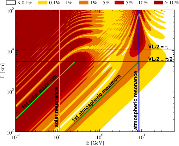
Figure 1: Contours of $P_{e\mu}$ calculated numerically without approximations for $\sin^{2}2\theta_{13}=0.02$, $\Delta m_{31}^{2}=2\cdot 10^{-3}\,{\rm eV}^{2}$, $\alpha=0.03$, $\theta_{12}=33^{\circ}$, $\theta_{23}=45^{\circ}$, and $\delta_{\rm CP}=0$. Matter of constant density $\rho=3\,{\rm g/cm^{3}}$ is assumed, and the probability is averaged over a Gaussian energy resolution of 1%.

Many features of this figure can be understood by considering the expression for the two-flavor neutrino oscillation probability in matter of constant density:

$$P=\frac{\sin^{2}2\theta}{C^{2}}\sin^{2}C\Delta_{2\nu}\,,\qquad C\equiv\sqrt{\sin^{2}2\theta+(\cos 2\theta-A_{2\nu})^{2}}\,,$$ (76)

where, in analogy to Eqs. (25) and (26), we define $\Delta_{2\nu}\equiv\Delta m^{2}L/(4E)$, $A_{2\nu}\equiv 2EV/\Delta m^{2}$, and $\theta$ and $\Delta m^{2}$ are the generic two-flavor neutrino oscillation parameters. From Eq. (76) it is clear that for $A_{2\nu}\ll 1$ one has $C\simeq 1$, and vacuum neutrino oscillations with $P\simeq\sin^{2}2\theta\sin^{2}\Delta_{2\nu}$ are recovered. For $A_{2\nu}=\cos 2\theta$ one can see in Eq. (76) also the MSW resonance [25], which leads to $C=\sin 2\theta$ in Eq. (76) and to the effective mixing angle in matter $\sin^{2}2\theta^{\prime}=\sin^{2}2\theta/C^{2}=1$. The general resonance conditions for three flavors are much more complicated than those in the two-flavor case. However, due to the hierarchy of the mass squared differences and smallness of $\theta_{13}$, one can use, to a very good approximation, the respective effective two-flavor picture. This leads to the “solar” and “atmospheric” resonance energies shown as vertical lines in Fig. 1

$$\frac{A}{\alpha}=\frac{2EV}{\Delta m^{2}_{21}}=\cos 2\theta_{12}\,,\qquad A=\frac{2EV}{\Delta m^{2}_{31}}=\cos 2\theta_{13}\,.$$ (77)

The “atmospheric” resonance is clearly visible in Fig. 1 at $E_{\mathrm{res}}\simeq 8.6$ GeV and $L\gtrsim 5500$ km. The “solar” resonance occurs at the energy $E_{\mathrm{res}}\simeq 0.11$ GeV. Note that the solar resonance is not as pronounced in Fig. 1 as the atmospheric one, since the neutrino oscillation amplitude in vacuum $\sin^{2}2\theta_{12}$ is already quite large.

Far enough to the left of the vertical lines in Fig. 1 marking the solar and atmospheric resonance energies one has vacuum neutrino oscillations with the “solar” parameters $\theta_{12}$, $\Delta m^{2}_{21}$ and with the “atmospheric” parameters $\theta_{13}$, $\Delta m^{2}_{31}$, respectively. Indeed, the typical $L/E$ pattern is clearly visible in Fig. 1 to the left of the vertical lines. The diagonal lines indicate the constant values of $L/E$ corresponding to the first solar and atmospheric oscillation maxima in vacuum, given by the conditions

$$\alpha\Delta=\frac{\Delta m_{21}^{2}L}{4E}=\frac{\pi}{2}\,,\qquad\Delta=\frac{\Delta m_{31}^{2}L}{4E}=\frac{\pi}{2}\,,$$ (78)

respectively. To the right of the vertical lines the probability is dominated by matter effects. For $A_{2\nu}\gg 1$ we have $C\simeq A_{2\nu}$ in Eq. (76), which has two consequences: First, since $A_{2\nu}\Delta_{2\nu}=VL/2$, the oscillation frequency becomes independent of energy, and second, the oscillation amplitude becomes suppressed at high energies because $\sin^{2}2\theta/A_{2\nu}^{2}\propto 1/E^{2}$. Both these effects are apparent in Fig. 1 for neutrino oscillations with the solar as well as the atmospheric frequency.

In addition to the dependence on the neutrino energy, matter effects depend crucially on the baseline. From Eq. (76) one can see that the two-flavor oscillation probabilities approach the vacuum ones for $C\Delta_{2\nu}\ll\pi/2$. Far above the MSW resonance energy, i.e.  for $A_{2\nu}\gg 1$, one finds $C\simeq A_{2\nu}$. Hence, the short-baseline limit is $C\Delta_{2\nu}\simeq A_{2\nu}\Delta_{2\nu}=VL/2\ll\pi/2$, leading to vanishing matter effects for $L\ll L_{\mathrm{mat}}\equiv\pi/V\simeq 5453$ km. The horizontal lines in Fig. 1 indicate this baselines of the first “matter effect maximum” for large energies at $L=L_{\mathrm{mat}}$, and the first “matter effect minimum”, $L=2L_{\mathrm{mat}}\simeq 10907$ km. At the baseline $2L_{\mathrm{mat}}$, where $A\Delta=VL/2=\pi$, the terms proportional to $\alpha^{2}$ and $\alpha s_{13}$ in the double expansion Eq. (31) disappear, and only the term proportional to $s_{13}^{2}$ survives. Therefore, this baseline is especially useful to measure $s_{13}$, since ambiguities due to parameter degeneracies are avoided [38]. A dedicated analysis of this “magic baseline” can be found in Ref.[46]. Note that the distance $L_{\mathrm{mat}}$ depends only on the matter potential $V$, i.e. the energy $E$ as well as neutrino masses and mixings do not enter.

Let us now consider the energy region well below the MSW resonance energy, where $A_{2\nu}\ll 1$. The short-baseline behavior of the oscillation probability in this region can be understood in the two-flavor picture by expanding Eq. (76) for fixed $\Delta_{2\nu}$ (i.e., fixed $L/E$) assuming $A_{2\nu}\ll 1$ and $\Delta_{2\nu}A_{2\nu}\ll 1$. One finds

$$P^{\mathrm{matter}}-P^{\mathrm{vacuum}}\simeq 2\sin^{2}2\theta\cos 2\theta\>\sin\Delta_{2\nu}\left(\sin\Delta_{2\nu}-\Delta_{2\nu}\cos\Delta_{2\nu}\right)A_{2\nu}\,.$$ (79)

This relation shows that $P^{\mathrm{matter}}-P^{\mathrm{vacuum}}$ decreases linearly with $A_{2\nu}\propto E$, which means that the matter effects vanish for very small energies, as mentioned above. In addition, for a fixed energy the right-hand side of Eq. (79) becomes zero for $\Delta_{2\nu}\ll 1$ or, equivalently, $L\ll L_{\mathrm{vac}}\equiv 4\pi E/\Delta m^{2}$. Therefore, the two conditions for the smallness of matter effects due to the short baseline can be written for all energies as $L\ll L_{\mathrm{min}}\equiv\mathrm{min}(L_{\mathrm{vac}},L_{\mathrm{mat}})$.

The relevance of matter effects is illustrated in Fig. 2. In the upper left panel we show the probability difference $|P_{e\mu}^{\mathrm{matter}}-P_{e\mu}^{\mathrm{vacuum}}|$ for the case $\alpha=0$, such that the oscillations due to the “solar” frequency are switched off and only matter effects are present which are related to the “atmospheric” resonance energy at 8.6 GeV. It can be seen that the difference, as well as the relative difference (lower left panel), vanish for $L\ll L_{\mathrm{min}}$.

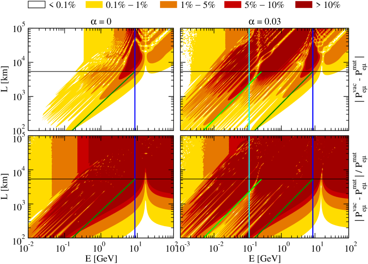
Figure 2: Contours of $|P_{e\mu}^{\mathrm{matter}}-P_{e\mu}^{\mathrm{vacuum}}|$ (upper panels), and $|P_{e\mu}^{\mathrm{matter}}-P_{e\mu}^{\mathrm{vacuum}}|/P_{e\mu}^{\mathrm{matter}}$ (lower panels), where $P_{e\mu}^{\mathrm{matter}}$ ($P_{e\mu}^{\mathrm{vacuum}}$) is the exact oscillation probability in matter (vacuum) for $\sin^{2}2\theta_{13}=0.05$, $\Delta m_{31}^{2}=2\cdot 10^{-3}\,{\rm eV}^{2}$, and $\theta_{23}=45^{\circ}$. In the left panels $\alpha=0$, whereas in the right panels $\alpha=0.03$, $\theta_{12}=33^{\circ}$, and $\delta_{\rm CP}=0$. Matter of constant density $\rho=3\,{\rm g/cm^{3}}$ is assumed, and the probabilities are averaged over a Gaussian energy resolution of 2%. The straight lines indicate the relevant resonance energies, first oscillation maxima, and the first matter effect maximum (see also Fig. 1).

The left plots of Fig. 2 show that the differences vanish also for small energies and long baselines. This can be understood as follows. For $E\ll E_{\rm res}$ the oscillation amplitude in matter is always close to that in vacuum. For very short baselines, this is also true for the oscillation phases. At intermediate baselines, the matter-induced correction to the oscillation phase, though much smaller than the main “vacuum” term, can become comparable to unity and so cannot be ignored. However, at long baselines $L\gg L_{\mathrm{vac}}$ the averaging regime sets in, which implies that any shifts in the oscillation phase become unimportant and the vacuum oscillations limit is regained.

The above discussion describes the regions where $|P_{e\mu}^{\mathrm{matter}}-P_{e\mu}^{\mathrm{vacuum}}|$ vanishes or becomes small for $\alpha=0$ in the left plots of Fig. 2. One can also understand in this way why the difference $|P_{e\mu}^{\mathrm{matter}}-P_{e\mu}^{\mathrm{vacuum}}|$ disappears more slowly towards low $E$ and $L$ along the lines of constant $L/E$ in the upper left plot of Fig. 2. The structures seen in the plot emerge from the matter dependent phase shifts of oscillation probabilities with more or less equal amplitudes. This behavior can be understood in the two-flavor picture from Eq. (79), which implies that $P^{\mathrm{matter}}-P^{\mathrm{vacuum}}$ grows linearly with $E$ along the lines of constant $\Delta_{2\nu}$ or, equivalently, constant $L/E$. This growth is modulated in the $\Delta_{2\nu}$-direction by the factor $\sin\Delta_{2\nu}\left(\sin\Delta_{2\nu}-\Delta_{2\nu}\cos\Delta_{2\nu}\right)$, which describes nicely the details of the structures extending along lines of constant $\Delta_{2\nu}$ towards lower energies.

The right plots of Fig. 2 show the probability difference $|P_{e\mu}^{\mathrm{matter}}-P_{e\mu}^{\mathrm{vacuum}}|$ and the relative difference for the case $\alpha=0.03$. This figure contains the structures stemming from the atmospheric resonance energy, which were already present in the $\alpha=0$ case (left plots). In addition, similar structures show up around the solar resonance energy, reaching to lower energies and, due to the larger effective mixing angle, also to shorter baselines. The right plots of Fig. 2 show that in the realistic case of two mass squared differences matter effects are rather important and have to be taken into account in a large domain of the physically interesting parameter space.

6.2 Comparing the accuracy of the three types of expansions

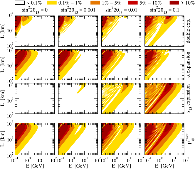
Figure 3: Rows 1, 2, and 3: absolute errors of the three types of expansions for $P_{e\mu}$ as functions of neutrino energy $E$ and baseline length $L$, for $\Delta m_{31}^{2}=2\cdot 10^{-3}\,{\rm eV}^{2}$, $\alpha=0.03$, $\theta_{12}=33^{\circ}$, $\theta_{23}=45^{\circ}$, $\delta_{\rm CP}=0$, and several values of $\sin^{2}2\theta_{13}$. Matter of constant density $\rho=3\,{\rm g/cm^{3}}$ is assumed. Row 4 shows contours of $P_{e\mu}$ calculated numerically.

In order to test the accuracy of our analytic expressions, we shall now compare the values of $P_{e\mu}$ obtained from the expansion formulas Eq. (31) for the double expansion, Eqs. (47) and (48) for the single expansion in $\alpha$, and Eqs. (65) and (66) for the single expansion in $s_{13}$ with the exact values of $P_{e\mu}$ calculated numerically. Figure 3 shows the absolute errors $|P_{e\mu}^{\mathrm{expansion}}-P_{e\mu}^{\mathrm{exact}}|$, and Fig. 4, the relative errors $|P_{e\mu}^{\mathrm{expansion}}-P_{e\mu}^{\mathrm{exact}}|/P_{e\mu}^{\mathrm{exact}}$ for the three types of expansions as functions of the neutrino energy $E$ and baseline length $L$ for various values of $\sin^{2}2\theta_{13}$. For reference, we display in the lowest row of graphs in each of these figures also the probability $P_{e\mu}$ itself, calculated numerically without any approximations.

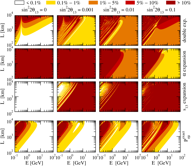
Figure 4: Rows 1, 2, and 3: relative errors of the three types of expansions for $P_{e\mu}$ as functions of neutrino energy $E$ and baseline length $L$, for $\Delta m_{31}^{2}=2\cdot 10^{-3}\,{\rm eV}^{2}$, $\alpha=0.03$, $\theta_{12}=33^{\circ}$, $\theta_{23}=45^{\circ}$, $\delta_{\rm CP}=0$, and several values of $\sin^{2}2\theta_{13}$. Matter of constant density $\rho=3\,{\rm g/cm^{3}}$ is assumed. Row 4 shows contours of $P_{e\mu}$ calculated numerically.

First, we observe that in general the absolute errors shown in Fig. 3 are rather small—at the 0.1% level in a large part of the parameter space, whereas the relative errors shown in Fig. 4 are considerably larger, due to the smallness of the probability itself. Next, we note that the series expansions in $\alpha$, i.e., the double expansion in $\alpha$ and $s_{13}$ and the single expansion in $\alpha$, are only valid for

$$\alpha\Delta=\frac{\Delta m_{21}^{2}L}{4E}\ll 1\,,\qquad\mbox{or}\qquad\frac{L}{E}\ll{10^{4}\;\mathrm{km}/\mathrm{GeV}}\,,$$ (80)

i.e., far below the first solar maximum. The obvious reason is that expanding terms of the type $\sin\alpha\Delta$ is only valid if $\alpha\Delta$ is small, and hence, these two types of expansion cannot account for neutrino oscillations with the “solar” frequency. Note that for $s_{13}=0$ the single expansion in $\alpha$ gives $P_{e\mu}=0$, since in that case the lowest-order term of $P_{e\mu}$ is proportional to $\alpha^{2}$, and our single expansion in $\alpha$ only contains terms up to first order in $\alpha$. This explains why at very small values of $s_{13}$ the double expansion (which includes terms of second order in $\alpha$) is more accurate than the single expansion in $\alpha$. In contrast, the neutrino oscillations with the “solar” frequency (for which the condition in Eq. (80) is violated) are in general very well accounted for by the single expansion in $s_{13}$, since it retains the exact dependence of the probability on $\alpha$. This expansion is the best one for relatively small values of $s_{13}$ and large values of $L/E$.

Figures 3 and 4 allow us to put the above observations on a more quantitative basis. In the region of $L/E$ given in Eq. (80) (lower-right parts of the graphs), where the oscillations are mainly driven by the “atmospheric” mass squared difference $\Delta m^{2}_{31}$, the double expansion and the single expansion in $\alpha$ work rather well. For not too large values of $\sin^{2}2\theta_{13}$ the double expansion is most accurate, with absolute errors at the 0.1% level and relative errors not exceeding 1% (5%) for $\sin^{2}2\theta_{13}=0.001\,(0.01)$. However, for values of $\sin^{2}2\theta_{13}$ close to the current upper bound the single expansion in $\alpha$ becomes better, with relative errors smaller than 1%. The reason for this is that for large values of $\sin^{2}2\theta_{13}$ the neutrino oscillations driven by the “atmospheric” frequency and mixing angle $\theta_{13}$ completely dominate the probability, and, in addition, for relatively large values of $L$ and energies close to 10 GeV, the atmospheric resonance becomes important. Since the single expansion in $\alpha$ is exact in $s_{13}$, it describes the case of relatively large $s_{13}$ well, and the atmospheric resonance is also correctly accounted for. At the same time, the accuracy of the double expansion becomes slightly worse near the first atmospheric maximum and the resonance. As was pointed out in Ref.[36], for large values of $s_{13}$ the accuracy of the double expansion can be improved by replacing the term proportional to $s_{13}^{2}$ in Eq. (31) by the term given in Eq. (47) as the zeroth order term in the single expansion in $\alpha$. For $\alpha=0$ this term describes the probability $P_{e\mu}$ exactly to all orders in $s_{13}$.

As can be seen from Figs. 3 and 4, the single expansion in $s_{13}$ gives a rather poor description of the region of $L/E$ defined in Eq. (80). The reason is that with only terms of first order in $s_{13}$ it is not possible to obtain a correct description of neutrino oscillations driven by $\Delta m^{2}_{31}$ and $\theta_{13}$. This is also reflected by the fact that the lowest-order in $s_{13}$ terms in the eigenvalues of the Hamiltonian are ${\cal O}(s_{13}^{2})$ [see Eqs. (27)–(29)]. On the other hand, the single expansion in $s_{13}$ is rather accurate for large values of $L/E$ violating the condition (80) (upper-left parts of the graphs) and relatively small values of $\theta_{13}$: for $\sin^{2}2\theta_{13}<0.001$ the accuracy is typically better than 1%.

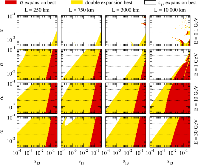
Figure 5: The plot shows which type of expansion for $P_{e\mu}$ is most accurate, depending on $\alpha$ and $s_{13}$ and for different values of neutrino energy $E$ and baseline length $L$. The values of the fundamental neutrino parameters used are $\Delta m_{31}^{2}=2\cdot 10^{-3}\,{\rm eV}^{2}$, $\theta_{12}=33^{\circ}$, $\theta_{23}=45^{\circ}$, and $\delta_{\rm CP}=0$. Matter of constant density $\rho=3\,{\rm g/cm^{3}}$ is assumed. The dotted lines indicate the $3\sigma$ allowed range of the parameter $\alpha$.

To conclude this subsection, we show in Fig. 5 which type of expansion provides the most accurate expression for $P_{e\mu}$, depending on the values of the expansion parameters $\alpha$ and $s_{13}$ and for a number of fixed values of neutrino energy $E$ and baseline length $L$. These plots change very little when the fundamental neutrino parameters $\Delta m_{31}^{2}$, $\theta_{12}$, $\theta_{23}$, and $\delta_{\rm CP}$ are varied within their allowed ranges, and also when one switches over to the other neutrino oscillation channels. As expected, one observes as a general trend that the single expansion in $\alpha$ is best for small $\alpha$ and large $s_{13}$, whereas the single expansion in $s_{13}$ is best for small $s_{13}$ and large $\alpha$. The double expansion is most accurate in a region where $\alpha$ and $s_{13}$ are of comparable order of magnitude.

In agreement with the discussion related to Figs. 3 and 4, we find from Fig. 5 that in the low-energy regime $E\sim 0.1$ GeV the single expansion in $s_{13}$ is most accurate in almost the entire $\alpha$-$\theta_{13}$ plane. For values of $L/E$ satisfying the condition (80) and energies larger than a few GeV the double expansion is most accurate in a large fraction of the $\alpha$-$\theta_{13}$ plane; only for values of $s_{13}$ close to the current upper bound does the single expansion in $\alpha$ become better. Furthermore, we note that for $E\sim 10$ GeV and $L\gtrsim 5500$ km the atmospheric resonance is important, which leads to a better accuracy of the single expansion in $\alpha$ (see the rightmost panel in the third row of Fig. 5).

We conclude that the double expansion in both $\alpha$ and $s_{13}$ is most accurate in a wide region of the parameter space, where $\alpha$ and $s_{13}$ are roughly of the same order of magnitude. The single expansion in $s_{13}$ has to be used whenever neutrino oscillations with the solar frequency are important (e.g., in the low-energy regime), whereas the single expansion in $\alpha$ is most accurate for values of $s_{13}$ close to the upper bound, or in cases where the atmospheric resonance is important.

6.3 Accuracy of the double expansion

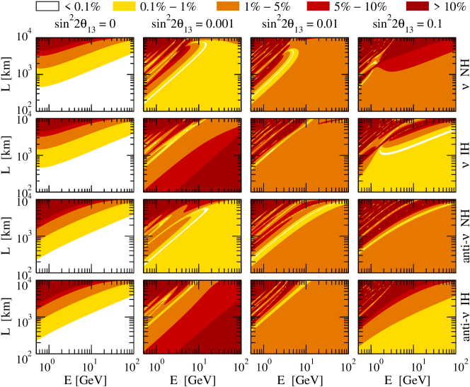
Figure 6: Relative errors of the double expansion for $P_{e\mu}$ for neutrinos (rows 1 and 2), and $P_{\overline{e}\overline{\mu}}$ for antineutrinos (rows 3 and 4), for normal hierarchy (NH) and inverted hierarchy (IH). The values of the fundamental neutrino parameters used are $|\Delta m_{31}^{2}|=2\cdot 10^{-3}\,{\rm eV}^{2}$, $\alpha=0.03$, $\theta_{12}=33^{\circ}$, $\theta_{23}=45^{\circ}$, $\delta_{\rm CP}=0$, and several values of $\sin^{2}2\theta_{13}$. Matter of constant density $\rho=3\,{\rm g/cm^{3}}$ is assumed.

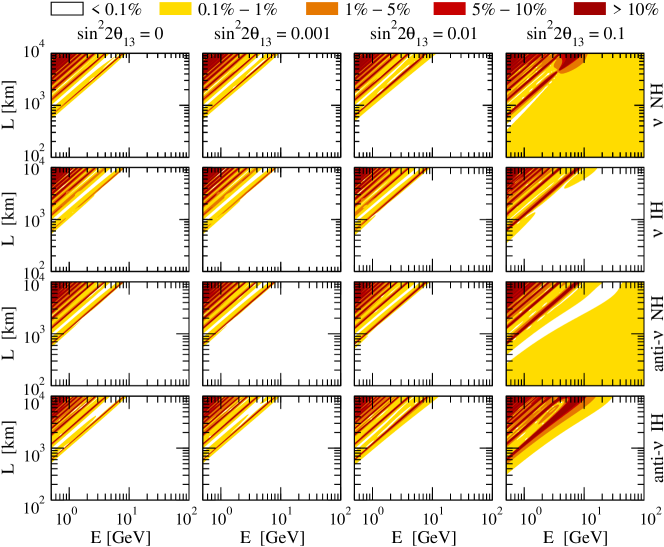
Figure 7: Relative errors of the double expansion for $P_{\mu\tau}$ for neutrinos (rows 1 and 2), and $P_{\overline{\mu}\overline{\tau}}$ for antineutrinos (rows 3 and 4), for normal hierarchy (NH) and inverted hierarchy (IH). The values of the fundamental neutrino parameters used are $|\Delta m_{31}^{2}|=2\cdot 10^{-3}\,{\rm eV}^{2}$, $\alpha=0.03$, $\theta_{12}=33^{\circ}$, $\theta_{23}=45^{\circ}$, $\delta_{\rm CP}=0$, and several values of $\sin^{2}2\theta_{13}$. Matter of constant density $\rho=3\,{\rm g/cm^{3}}$ is assumed.

Motivated by the fact that the double expansion is most accurate in a wider region of the parameter space than the single expansions, we present in this subsection some more accuracy tests for it. Figures 6 and 7 show the relative errors for $P_{e\mu}$ given in Eq. (31) and $P_{\mu\tau}$ given in Eq. (34), respectively, for neutrinos, antineutrinos, and normal and inverted hierarchies. We note that the relative accuracy of $P_{e\tau}$ and $1-P_{ee}$ is very similar to the one of $P_{e\mu}$ (Fig. 6), and the accuracy of $P_{\mu\mu}$ and $P_{\tau\tau}$ is similar to that of $P_{\mu\tau}$ (Fig. 7).

In the region of $L/E$ defined in Eq. (80), the accuracy of $P_{e\mu}$ is roughly between 1% and 5%. It should be noted that the absolute errors of the double expansion of $P_{e\mu}$ depend very weakly on the choice of the fundamental neutrino parameters within their allowed ranges, and they are always very small, similar to the first row of plots in Fig. 3. However, the relative errors shown in Fig. 6 are rather sensitive to the fundamental parameters values in the region of low $L/E$. The reason is that the probability $P_{e\mu}$ itself is typically very small in this region, being as tiny as $10^{-7}$, or even smaller. Hence, the relative error, being a ratio of two small numbers, is quite sensitive to variations of the parameters (see, e.g., the second column in Fig. 6). In contrast, $P_{\mu\tau}$ is rather large, because of the oscillations in “atmospheric” channel driven by the large $\Delta m_{31}^{2}$ and maximal or nearly maximal mixing $\sin^{2}2\theta_{23}\simeq 1$. This is also clear from Eq. (34), since $P_{\mu\tau}$ has a term of zeroth order in both $\alpha$ and $s_{13}$, while $P_{e\mu}$ from Eq. (31) is of second order in these parameters. Hence, in the case of $P_{\mu\tau}$, the relative errors are of the same order as the absolute errors, which are always very small. The errors shown in Fig. 7 are smaller than 0.1% for $\sin^{2}2\theta_{13}\leq 0.01$ and smaller than 1% for $\sin^{2}2\theta_{13}\leq 0.1$.

6.4 Probability expansions and relation to experiments

The discussion of the accuracy of the different expansions can be used to identify the best set of equations for a given neutrino oscillation experiment. The first question is, however, whether matter effects are relevant or if the much simpler vacuum probabilities can be used. The absolute and relative differences between matter and vacuum probabilities vanish, as discussed in Sec. 6.1, for sufficiently low energies or for short enough baselines. The discussion showed that in experimentally interesting cases matter effects are almost always relevant for the ranges of $L$ and $E$ that we considered. If $L/E$ is such that oscillations can be observed, then for fixed $L/E$ the matter effects are negligible only at very small $E$ (and consequently small $L$). An example where matter effects can be ignored at the percent level is given by the reactor $\bar{\nu}_{e}$ disappearance experiments with energies of a few MeV and baselines up to a few kilometers.

In order to identify the best expansion for a given experiment, one must take into account that the analyses of real experiments are based on event rates and not on probabilities. It is useful to distinguish here between “point sources” (accelerator beams, reactors, the Sun, supernovae, etc.) where the observed neutrinos come from one point-like region in space, and “extended sources” (e.g., the atmosphere) where the observed neutrinos come from many different positions in space. An event rate based analysis of point sources implies essentially, for a given energy, an additional factor $1/L^{2}$ in order to account for the reduction of the flux as a function of the baseline $L$. In addition, the detection cross section is typically proportional to $E^{r}$, where $1\lesssim r\lesssim 2$, depending on the energy range and on the detection process. In the two-flavor approximation, when going from the first oscillation maximum at $\Delta_{2\nu}=\pi/2$ to the $n$th oscillation maximum at $\Delta_{2\nu}=(n-1/2)\pi$ this implies that the event rates drop by a factor $1/(2n-1)^{2}$ if the baseline is increased, or by a factor $1/(2n-1)^{r}$ if the energy is decreased. Hence, e.g., for a fixed energy the rate in the second (third) maximum is already reduced by a factor 1/9 (1/25). This explains why most current proposals for long baseline oscillation experiments aim at the first oscillation maximum of the “atmospheric” oscillations. The oscillations driven by the “solar” frequency are then a sub-leading effect, and in most cases the double expansion works very well. The overall relative precision of the double expansion is then typically in the range of a percent, or at worst, up to a few percent in this case. However, if $\theta_{13}$ is close to its current upper limit, the single expansion in $\alpha$ is even more precise than the double expansion. On the other hand, if $\theta_{13}$ is tiny, well below the sensitivity limits of any planned accelerator experiment, the single expansion in $s_{13}$ is more precise than the double expansion, especially for low energies. Note, however, that the double expansion has often a sufficient precision even when it is not the best expansion.

The discussion of point sources does not change much for experiments which aim at higher oscillation maxima. The $1/(2n-1)^{2}$ flux factor due to the beam divergence and/or the $1/(2n-1)^{r}$ factor due to the energy dependence of the detection cross sections reduce the observed event rates and limit all proposals to the first few oscillation maxima at best. The double expansion still works quite well for such proposals, as long as the sub-leading oscillations governed by the “solar” frequency stay in the linear regime, where an expansion in $\alpha$ makes sense. This leads to the condition $2n-1\ll\alpha^{-1}\simeq 40$, which is fulfilled for the first few maxima. Higher values of $n$ are currently not proposed, since the flux and/or cross section would drop by a large factor, which would make the detectors and sources unaffordable. For largest (smallest) $\theta_{13}$ the single expansion in $\alpha$ ($s_{13}$) works again numerically even better then the double expansion, just like in the case of the first oscillation maximum.

The discussion is somewhat different for sources which are not point-like. In that case, there is in general no $1/L^{2}$ suppression of the flux, and the observed event rates are not dominated by the first oscillation maximum. An important example are atmospheric neutrinos, for which a wide range of baselines and energies contributes: the energy window of practical interest ranges from a 100 MeV to a few tens of GeV, while the baseline lies between $10$ km and $10^{4}$ km. This wide range of energies and baselines makes clear that none of the discussed expansions covers the full parameter range at the percent level. In general the double expansion works quite well for small or moderate $L/E$, while the $s_{13}$ expansion tends to work best for larger $L/E$ values. At the same time, close to the atmospheric resonance or if the mixing angle $\theta_{13}$ is near its current upper bound and for not too large $L/E$, the $\alpha$ expansion is expected to be the most relevant one.

In general, for all types of experiments and for any given values of $L$, $E$, and $\theta_{13}$ the most accurate expansion can readily be found with the help of Fig. 5.

7 Summary and conclusions

In this paper we have presented three different sets of approximate formulas for the probabilities of neutrino oscillations in matter and in vacuum. We have shown that in general the probabilities for all possible oscillation channels for neutrinos as well as for antineutrinos can be obtained from just two independent probabilities by using unitarity and a symmetry related to the “atmospheric” mixing angle $\theta_{23}$ [see Eq. (14)]. One possible choice for these two probabilities is $P_{e\mu}$ and $P_{\mu\tau}$. We have derived the expressions for the neutrino oscillation probabilities in matter of constant density, expanded in terms of the small parameters $\alpha\equiv\Delta m^{2}_{21}/\Delta m^{2}_{31}$, $s_{13}$ or in both of them. Below we summarize the main features of these expansions:

• Double expansion up to second order in $\alpha$ and $s_{13}$ [Sec. 3.1, Eqs. (30)–(34)]

  The neutrino oscillation probabilities are expanded in both small parameters up to second order. In general, these expressions are valid for $\alpha\Delta=\Delta m_{21}^{2}L/(4E)\ll 1$ or $L/E\ll 10^{4}\,\mathrm{km}/\mathrm{GeV}$, i.e., if neutrino oscillations due to the solar mass squared difference $\Delta m^{2}_{21}$ are not important. The accuracy of the approximation is good for a wide range of the parameters. Typically, the relative errors of $P_{e\mu}$, $P_{e\tau}$, and $1-P_{ee}$ are between 1% and 5%, the relative errors of $P_{\mu\mu}$, $P_{\mu\tau}$, and $P_{\tau\tau}$ and the absolute errors for all probabilities are of the order 0.1%.

• Single expansion up to first order in $\alpha$ [Sec. 4.1, Eqs. (45)–(50)]

  The neutrino oscillation probabilities are expanded in $\alpha$, but the exact dependence on $s_{13}$ is retained. Like in the case of the double expansion, these formulas are valid in the region where the oscillations driven by the solar mass squared difference are not important: $\alpha\Delta=\Delta m_{21}^{2}L/(4E)\ll 1$, or $L/E\ll 10^{4}\,\mathrm{km}/\mathrm{GeV}$. The accuracy is better than the one of the double expansion for values of $s_{13}\gtrsim 0.1$ close the current upper bound, or if the atmospheric resonance is important. For instance, for a matter density $\rho=3\,{\rm g/cm^{3}}$ and $\Delta m^{2}_{31}=2\cdot 10^{-3}\,{\rm eV}^{2}$ this is the case for $E\sim 10$ GeV and $L\gtrsim 5500$ km.

• Single expansion up to first order in $s_{13}$ [Sec. 5.1, Eqs. (63)–(68)]

  The neutrino oscillation probabilities are expanded in $s_{13}$, but the exact dependence on $\alpha$—and therefore on $\Delta m^{2}_{21}$—is retained. Hence, these expressions are useful in the region where the oscillations due to the solar mass squared difference are relevant: $\alpha\Delta=\Delta m_{21}^{2}L/(4E)\gtrsim 1$, or $L/E\gtrsim 10^{4}\,\mathrm{km}/\mathrm{GeV}$. In particular, this is the case for low energies $E\sim 0.1$ GeV and $L\gtrsim 10^{3}$ km. For values of $L/E$ outside the “solar” regime this type of expansion is only useful for very small values of $s_{13}\lesssim 10^{-4}\div 10^{-3}$.

• Vacuum limit of the expansions [Secs. 3.2, 4.2, 5.2]

  The vacuum limit for each type of expansion is valid if, in addition to the requirements ensuring the validity of a given type of expansion, matter effects can be neglected (see discussion in Sec. 6.1). This usually implies low energies or short baselines. We find that in many realistic cases matter effects are of the order of a few percent. Hence, if an accuracy at that level is required, one should employ the formulas for neutrino oscillations in matter.

In conclusion, we have presented a collection of formulas for three-flavor neutrino oscillation probabilities by deriving expansions in small parameters. We have performed a detailed analysis of the accuracy of these expansions and determined the parameter regions where they are most accurate. The expansions of the neutrino oscillation probabilities in matter of constant density are useful for the analytical understanding of the physics of future neutrino oscillation experiments. Furthermore, we have also presented expansion formulas for the neutrino oscillation probabilities in arbitrary matter density profiles (see Appendix B), which can be applied to a large class of problems.

Acknowledgments

We would like to thank Martin Freund, Håkan Snellman, and Walter Winter for useful discussions and comments. T.S. thanks the KTH for hospitality and financial support for a research visit. R.J. and T.O. would like to thank the TUM for the warm hospitality during their research visits as well as for the financial support. E.A. was supported by the sabbatical grant SAB2002-0069 of the Spanish Ministry of Education, Culture, and Sports, the RTN grant HPRN-CT-2000-00148 of the European Commission, the ESF Neutrino Astrophysics Network and MCyT grant BFM2002-00345. M.L. and T.S. were supported by the “Sonderforschungsbereich 375 für Astro-Teilchenphysik der Deutschen Forschungsgemeinschaft”, and T.O. was supported by the Swedish Research Council (Vetenskapsrådet), Contract Nos. 621-2001-1611, 621-2002-3577, the Göran Gustafsson Foundation, and the Magnus Bergvall Foundation.

Appendix A Hamiltonian diagonalization approach

In this appendix, we present the details of the approximate diagonalization of the effective Hamiltonian of the neutrino system in the case of matter of constant density.

A.1 Diagonalizing the Hamiltonian perturbatively

In order to derive the double expansions given in Sec. 3, we write the Hamiltonian of Eq. (6) as

$$H\simeq\frac{\Delta m_{31}^{2}}{2E}O_{23}U_{\delta}\,M\,U_{\delta}^{\dagger}O_{23}^{T}\,,$$ (A1)

where $M\equiv O_{13}O_{12}\,\mathrm{diag}\left(0,\alpha,1\right)O_{12}^{T}O_{13}^{T}+\mathrm{diag}\left(A,0,0\right)$, and the matrices $O_{ij}$ and $U_{\delta}$ have been defined after Eq. (1). The matrix $M$ can be explicitly written as $M=(\Delta m_{31}^{2}/2E)^{-1}H^{\prime}$ by setting $\delta_{\mathrm{CP}}=0$ in $H^{\prime}$, which is given in Eq. (B1) below. First, we diagonalize the matrix $M$ by $M=W\hat{M}W^{\dagger}$ with $\hat{M}=\mathrm{diag}(\lambda_{1},\lambda_{2},\lambda_{3})$ and $W$ being a unitary diagonalizing matrix. This diagonalization is performed by using perturbation theory up to second order in the small parameters $\alpha$ and $s_{13}$, i.e., we write $M=M^{(0)}+M^{(1)}+M^{(2)}$, where $M^{(1)}$ ($M^{(2)}$) contains all terms of first (second) order in $\alpha$ and $s_{13}$. One finds

$$M^{(0)} =\mathrm{diag}(A,0,1)=\mathrm{diag}(\lambda_{1}^{(0)},\lambda_{2}^{(0)},\lambda_{3}^{(0)})\,,$$ (A2)

$$M^{(1)} =\left(\begin{array}[]{ccc}\alpha s_{12}^{2}&\alpha s_{12}c_{12}&s_{13}\\ \alpha s_{12}c_{12}&\alpha c_{12}^{2}&0\\ s_{13}&0&0\end{array}\right)\,,$$ (A6)

$$M^{(2)} =\left(\begin{array}[]{ccc}s_{13}^{2}&0&-\alpha s_{13}s_{12}^{2}\\ 0&0&-\alpha s_{13}s_{12}c_{12}\\ -\alpha s_{13}s_{12}^{2}&-\alpha s_{13}s_{12}c_{12}&-s_{13}^{2}\end{array}\right)\,.$$ (A10)

For the eigenvectors we write $v_{i}=v_{i}^{(0)}+v_{i}^{(1)}+v_{i}^{(2)}$, and since $M^{(0)}$ is diagonal at zeroth order, we have $v_{i}^{(0)}=e_{i}$. Then, the first and second order corrections to the eigenvalues are given by

$$\lambda_{i}^{(1)} =M^{(1)}_{ii}\,,$$ (A11)

$$\lambda_{i}^{(2)} =M^{(2)}_{ii}+\sum_{j\neq i}\frac{\left(M^{(1)}_{ii}\right)^{2}}{\lambda_{i}^{(0)}-\lambda_{j}^{(0)}}\,,$$ (A12)

and the corrections to the eigenvectors are calculated by

$$v_{i}^{(1)} =\sum_{j\neq i}\frac{M^{(1)}_{ij}}{\lambda_{i}^{(0)}-\lambda_{j}^{(0)}}\>e_{j}\,,$$ (A13)

$$v_{i}^{(2)} =\sum_{j\neq i}\frac{1}{\lambda_{i}^{(0)}-\lambda_{j}^{(0)}}\left[M^{(2)}_{ij}+\left(M^{(1)}v_{i}^{(1)}\right)_{j}-\lambda^{(1)}_{i}\left(v_{i}^{(1)}\right)_{j}\right]e_{j}\,.$$ (A14)

The mixing matrix in matter is given by $U^{\prime}=O_{23}U_{\delta}W$ with $W=(v_{1},v_{2},v_{3})$, and the eigenvalues of the Hamiltonian [see Eqs. (27)–(29)] are obtained as $E_{i}=[\Delta m_{31}^{2}/(2E)]\lambda_{i}$ ($i=1,2,3$).

In our paper, we do not in general order the eigenvalues according to their magnitude. Such an ordering would create problems as one would have to re-label the eigenvalues upon passing through each of the two MSW resonances. The ordering is actually unimportant if one is careful to assign the correct eigenvector to each eigenvalue.

We also reiterate the point discussed at the end of Sec. 3.1: despite the fact that in the case of the double expansion the eigenvalues as well as certain entries of the leptonic mixing matrix in matter are divergent at $A\to 0$ and $A\to 1$, the neutrino oscillation probabilities are finite in these limits. In particular, the correct vacuum probabilities are recovered in the limit $A\to 0$. The mentioned divergences are of no concern to us, since we are interested in oscillation probabilities rather than in eigenvalues or the mapping between the mixing in matter and in vacuum, as was the case, e.g., in Ref. [36].

A.2 The Cayley-Hamilton formalism

In order to derive a series expansion for the evolution matrix $S$ in small parameters, we can use the following formula from Refs. [12, 14]:

$$S(t,t_{0}) ={\rm e}^{-\mathrm{i}HL}$$

$$=\frac{{\rm e}^{-\mathrm{i}E_{1}L}}{(E_{1}-E_{2})(E_{1}-E_{3})}\,\big{[}E_{2}E_{3}\mathbbm{1}_{3}-(E_{2}+E_{3})H+H^{2}\big{]}$$

$$+\frac{{\rm e}^{-\mathrm{i}E_{2}L}}{(E_{2}-E_{1})(E_{2}-E_{3})}\,\big{[}E_{1}E_{3}\mathbbm{1}_{3}-(E_{1}+E_{3})H+H^{2}\big{]}$$

$$+\frac{{\rm e}^{-\mathrm{i}E_{3}L}}{(E_{3}-E_{1})(E_{3}-E_{2})}\,\big{[}E_{1}E_{2}\mathbbm{1}_{3}-(E_{1}+E_{2})H+H^{2}\big{]}\,,$$ (A15)

where $H$ is the Hamiltonian in the flavor basis as given in Eq. (6) and $E_{i}$ ($i=1,2,3$) are the eigenvalues of this Hamiltonian. Inserting series expansions of the eigenvalues [see, e.g., Eqs. (40)–(42) and (58)–(60)] and the Hamiltonian $H$ into Eq. (A.2), it is straightforward to obtain an expression for $S_{\alpha\beta}$, and subsequently, for the neutrino oscillation probabilities $P_{\alpha\beta}=|S_{\beta\alpha}|^{2}$.

Appendix B Perturbative expansion of the evolution equation for arbitrary matter density profiles

In this appendix, we present the details of the perturbative expansion of the neutrino evolution equation in the case of matter with an arbitrary density profile. We also give the formulas relevant for the particular case of matter of constant density.

Consider the neutrino evolution matrix $S(t,t_{0})$ defined in Eq. (9). It is convenient to rotate it by the angle $\theta_{23}$ according to Eq. (13). The evolution matrix in the rotated basis $S^{\prime}(t,\,t_{0})$ satisfies the evolution equation ${\rm i}({\rm d}/{\rm d}t)S^{\prime}(t,t_{0})=H^{\prime}(t)S^{\prime}(t,t_{0})$ with the initial condition $S^{\prime}(t_{0},t_{0})=\mathbbm{1}$ and the Hamiltonian $H^{\prime}(t)$ given by [28]

$$H^{\prime}(t)=\left(\begin{array}[]{ccc}s_{12}^{2}c_{13}^{2}\Delta_{21}+s_{13}^{2}\Delta_{31}+V(t)&s_{12}c_{12}c_{13}\Delta_{21}&s_{13}c_{13}\left(\Delta_{31}-s_{12}^{2}\Delta_{21}\right){\rm e}^{-{\rm i}\delta_{CP}}\\ s_{12}c_{12}c_{13}\Delta_{21}&c_{12}^{2}\Delta_{21}&-s_{12}c_{12}s_{13}{\rm e}^{-{\rm i}\delta_{CP}}\Delta_{21}\\ s_{13}c_{13}\left(\Delta_{31}-s_{12}^{2}\Delta_{21}\right){\rm e}^{{\rm i}\delta_{CP}}&-s_{12}c_{12}s_{13}{\rm e}^{{\rm i}\delta_{CP}}\Delta_{21}&c_{13}^{2}\Delta_{31}+s_{12}^{2}s_{13}^{2}\Delta_{21}\end{array}\right).$$ (B1)

Here

$$\Delta_{21}\equiv\frac{\Delta m_{21}^{2}}{2E}\,,\qquad\Delta_{31}\equiv\frac{\Delta m_{31}^{2}}{2E}\,.$$ (B2)

It is important to notice that $H^{\prime}(t)$ [and hence, $S^{\prime}(t,t_{0})$] does not depend on the mixing angle $\theta_{23}$. This is a consequence of the specific parameterization of the leptonic mixing matrix $U$ in Eq. (1), in which the matrix $O_{23}$ is the leftmost one, and the fact that the matrix of the matter-induced potentials in the effective Hamiltonian $H(t)$ commutes with $O_{23}$. Once the matrix $S^{\prime}(t,t_{0})$ is found, one can use Eq. (13) to rotate back to the original flavor basis.

It is convenient to decompose the Hamiltonian $H^{\prime}(t)$ as $H^{\prime}(t)=H_{0}^{\prime}(t)+H_{I}^{\prime}$, where $H^{\prime}_{0}(t)$ is of zeroth order in some expansion parameter and $H_{I}^{\prime}$ is the remainder. Accordingly, the evolution matrix can be written as $S^{\prime}(t,t_{0})=S_{0}^{\prime}(t,t_{0})S_{1}^{\prime}(t,t_{0})$, where $S_{0}(t,t_{0})$ satisfies

$${\rm i}\frac{{\rm d}}{{\rm d}t}S_{0}^{\prime}(t,t_{0})=H_{0}^{\prime}(t)S_{0}^{\prime}(t,t_{0})\,,\qquad S_{0}^{\prime}(t_{0},t_{0})=\mathbbm{1}\,.$$ (B3)

Then the matrix $S_{1}^{\prime}(t,t_{0})$ satisfies

$${\rm i}\frac{{\rm d}}{{\rm d}t}S_{1}^{\prime}(t,t_{0})=[S_{0}^{\prime}(t,t_{0})^{-1}H_{I}^{\prime}S_{0}^{\prime}(t,t_{0})]S_{1}^{\prime}(t,t_{0})\,,\qquad S_{1}^{\prime}(t_{0},t_{0})=\mathbbm{1}\,.$$ (B4)

Up to now, no approximations have been made. Next, we shall find the evolution matrix perturbatively. Let $H_{1}^{\prime}$ be the part of $H_{I}^{\prime}$ that is of the first order in the chosen expansion parameter. Then, to first order in this parameter, one finds

$$S^{\prime}(t,t_{0})\simeq S_{0}^{\prime}(t,t_{0})-{\rm i}S_{0}^{\prime}(t,t_{0})\int_{t_{0}}^{t}[S_{0}^{\prime}(t^{\prime},t_{0})^{-1}H_{1}^{\prime}S_{0}^{\prime}(t^{\prime},t_{0})]\,{\rm d}t^{\prime}\,,$$ (B5)

from which, upon rotation back to the original flavor basis, the evolution matrix $S(t,t_{0})$ is obtained. We shall now consider the application of the above formalism to the cases when the expansion parameter is either $\alpha$ or $s_{13}$.

B.1 Expansion up to first order in $\alpha$

In this case, the zeroth-order Hamiltonian $H_{0}^{\prime}(t)$ is obtained from Eq. (B1) by taking the limit $\alpha\to 0$ (i.e., $\Delta_{21}\to 0$). The zeroth-order evolution matrix $S_{0}^{\prime}(t,t_{0})$ can then be written as [26]

$$S_{0}^{\prime}(t,t_{0})=\left(\begin{array}[]{ccc}u(t,t_{0})&0&v(t,t_{0})\,{\rm e}^{-{\rm i}\delta_{\rm CP}}\\ 0&f(t,t_{0})&0\\ -v^{*}(t,t_{0})\,{\rm e}^{{\rm i}\delta_{\rm CP}}&0&u^{*}(t,t_{0})\end{array}\right)\,,$$ (B6)

where $u(t,t_{0})$ and $v(t,t_{0})$ are to be found from the solution to the two-flavor problem governed by the mass squared difference $\Delta m_{31}^{2}$, mixing angle $\theta_{13}$, and matter potential $V(t)$, and

$$f(t,t_{0})=\exp\left[{{\rm i}\!\int_{t_{0}}^{t}\tilde{\Delta}(t^{\prime})\,{\rm d}t^{\prime}}\right]\,,\qquad\tilde{\Delta}(t)\equiv\frac{1}{2}\left[\frac{\Delta m_{31}^{2}}{2E}+V(t)\right]\,.$$ (B7)

The parameters $u$ and $v$ satisfy $|u|^{2}+|v|^{2}=1$. The factor ${\rm e}^{-{\rm i}\delta_{\rm CP}}$ was pulled out from $v$ for convenience (this will simplify some of the formulas given below).

The neutrino oscillation probabilities to first order in $\alpha$ in the case of matter with an arbitrary density profile can be written as

$$P_{ee} =|u|^{2}-2\,\frac{\alpha\Delta}{L}\,s_{12}^{2}\,{\rm Im}[uv^{*}\,(2\cos 2\theta_{13}\,I_{1}+\sin 2\theta_{13}\,I_{2})]\,,$$ (B8)

$$P_{e\mu} =s_{23}^{2}|v|^{2}+2\,\frac{\alpha\Delta}{L}\,s_{12}^{2}\,s_{23}^{2}\,{\rm Im}[uv^{*}\,(2\cos 2\theta_{13}\,I_{1}+\sin 2\theta_{13}\,I_{2})]+\frac{\alpha\Delta}{L}\,\sin 2\theta_{12}\sin 2\theta_{23}$$

$$\times\left\{\cos\delta_{\rm CP}\,{\rm Im}[v^{*}f^{*}(c_{13}I_{3}+s_{13}I_{4})]+\sin\delta_{\rm CP}\,{\rm Re}[v^{*}f^{*}(c_{13}I_{3}+s_{13}I_{4})]\right\}\,,$$ (B9)

$$P_{\mu\tau} =\frac{1}{4}\sin^{2}2\theta_{23}\,[1+|u|^{2}-2{\rm Re}(uf)]$$

$$-\frac{\alpha\Delta}{L}\,\sin^{2}2\theta_{23}\left\{s_{12}^{2}\,{\rm Im}\left[(u-f^{*})v^{*}\left(\cos 2\theta_{13}\,I_{1}+\frac{1}{2}\sin 2\theta_{13}\,I_{2}\right)\right]\right.$$

$$+\left.\left[c_{12}^{2}L-s_{12}^{2}\left(s_{13}^{2}\,I_{5}+c_{13}^{2}\,I_{6}-\frac{1}{2}\sin 2\theta_{13}\,I_{7}\right)\right]\,{\rm Im}(uf)\right\}$$

$$-\frac{\alpha\Delta}{L}\,\sin 2\theta_{12}\,\sin 2\theta_{23}\Big{\{}\cos\delta_{\rm CP}\big{[}c_{23}^{2}\,{\rm Im}[(u-f^{*})v^{*}(c_{13}\,I_{3}+s_{13}\,I_{4})]$$

$$+{\rm Im}[(c_{23}^{2}|u|^{2}-s_{23}^{2}-\cos 2\theta_{23}\,uf)\,(c_{13}\,I_{9}-s_{13}\,I_{8})]\big{]}$$

$$+\sin\delta_{\rm CP}\big{[}c_{23}^{2}\,{\rm Re}[(u-f^{*})v^{*}(c_{13}\,I_{3}+s_{13}\,I_{4})]$$

$$-{\rm Re}[(c_{23}^{2}|u|^{2}-s_{23}^{2}-\cos 2\theta_{23}\,uf)\,(c_{13}\,I_{9}-s_{13}\,I_{8})]\big{]}\Big{\}}\,,$$ (B10)

where the quantities $I_{1},I_{2},\ldots,I_{9}$ are given by

$$I_{1}\equiv\int_{t_{0}}^{t}u^{*}(t^{\prime},t_{0})v(t^{\prime},t_{0})\,\mathrm{d}t^{\prime}\,,\qquad I_{2}\equiv\int_{t_{0}}^{t}[v(t^{\prime},t_{0})^{2}-u^{*}(t^{\prime},t_{0})^{2}]\,\mathrm{d}t^{\prime}\,,$$

$$I_{3}\equiv\int_{t_{0}}^{t}u^{*}(t^{\prime},t_{0})f(t^{\prime},t_{0})\,\mathrm{d}t^{\prime}\,,\qquad I_{4}\equiv\int_{t_{0}}^{t}v(t^{\prime},t_{0})f(t^{\prime},t_{0})\,\mathrm{d}t^{\prime}\,,$$

$$I_{5}\equiv\int_{t_{0}}^{t}|u(t^{\prime},t_{0})|^{2}\,\mathrm{d}t^{\prime}\,,\qquad\qquad~{}~{}I_{6}\equiv\int_{t_{0}}^{t}|v(t^{\prime},t_{0})|^{2}\,\mathrm{d}t^{\prime}\,,$$

$$I_{7}\equiv\int_{t_{0}}^{t}[u(t^{\prime},t_{0})v(t^{\prime},t_{0})+u^{*}(t^{\prime},t_{0})v^{*}(t^{\prime},t_{0})]\,\mathrm{d}t^{\prime}\,,$$

$$I_{8}\equiv\int_{t_{0}}^{t}u^{*}(t^{\prime},t_{0})f^{*}(t^{\prime},t_{0})\,\mathrm{d}t^{\prime}\,,\qquad I_{9}\equiv\int_{t_{0}}^{t}v(t^{\prime},t_{0})f^{*}(t^{\prime},t_{0})\,\mathrm{d}t^{\prime}\,.$$

Note that the integrals $I_{5}$, $I_{6}$, and $I_{7}$ are real, $I_{5}+I_{6}=t-t_{0}$, and the integrals $I_{8}$ and $I_{9}$ can be obtained from $I_{3}$ and $I_{4}$, respectively, by substituting $f\to f^{*}$.

In the case of matter of constant density, the parameters $u$, $v$, and $f$ are given by

$$u(t,0) =\cos\frac{C_{13}\Delta\,t}{L}+{\rm i}\frac{\cos 2\theta_{13}-A}{C_{13}}\sin\frac{C_{13}\Delta\,t}{L}\,,$$ (B11)

$$v(t,0) =-{\rm i}\frac{\sin 2\theta_{13}}{C_{13}}\sin\frac{C_{13}\Delta\,t}{L}\,,$$ (B12)

$$f(t,0) =\exp\left[{{\rm i}\frac{(1+A)\Delta\,}{L}t}\right]\,.$$ (B13)

Inserting these expressions into the integrals $I_{1},I_{2},\ldots,I_{9}$ and the obtained results into Eqs. (B8)–(B10) leads to Eqs. (45)–(50).

B.2 Expansion up to first order in $s_{13}$

This case was studied in detail in Ref. [28] (Appendix A), which we closely follow here. The zeroth-order Hamiltonian $H_{0}^{\prime}(t)$ is obtained from Eq. (B1) by taking the limit $\theta_{13}\to 0$. The zeroth-order evolution matrix $S_{0}^{\prime}(t,t_{0})$ can be written as

$$S_{0}^{\prime}(t,t_{0})=\left(\begin{array}[]{ccc}x(t,t_{0})&y(t,t_{0})&0\\ -y^{*}(t,t_{0})&x^{*}(t,t_{0})&0\\ 0&0&g(t,t_{0})\end{array}\right)\,,$$ (B14)

where $x(t,t_{0})$ and $y(t,t_{0})$ are to be found from the solution to the two-flavor problem governed by the mass squared difference $\Delta m_{21}^{2}$, mixing angle $\theta_{12}$, and matter potential $V(t)$, and

$$g(t,t_{0})=\exp\left[{-{\rm i}\!\int_{t_{0}}^{t}\hat{\Delta}(t^{\prime})\,{\rm d}t^{\prime}}\right]\,,\qquad\hat{\Delta}(t)\equiv\frac{\Delta m_{31}^{2}}{2E}-\frac{1}{2}\left[\frac{\Delta m_{21}^{2}}{2E}+V(t)\right]\,.$$ (B15)

The parameters $x$ and $y$ satisfy $|x|^{2}+|y|^{2}=1$.

The neutrino oscillation probabilities to first order in $s_{13}$ in the case of matter with an arbitrary density profile can be written as

$$P_{ee} =|x|^{2}\,,$$ (B16)

$$P_{e\mu} =c_{23}^{2}\,|y|^{2}-\sin 2\theta_{23}\,{\rm Im}(ygC)\,,$$ (B17)

$$P_{\mu\tau} =s_{23}^{2}c_{23}^{2}\,|x-g^{*}|^{2}+\sin 2\theta_{23}\,{\rm Im}[(x-g^{*})g(s_{23}^{2}B-c_{23}^{2}D)]\,,$$ (B18)

where the quantities $B$,$C$, and $D$ are defined as [47]

$$B\equiv B(t,t_{0}) =aI_{y^{*},t}(t,t_{0})+bI_{x,t}(t,t_{0})\,,$$ (B19)

$$C\equiv C(t,t_{0}) =a^{*}I^{*}_{x^{*},t_{0}}(t,t_{0})-b^{*}I^{*}_{y,t_{0}}(t,t_{0})\,,$$ (B20)

$$D\equiv D(t,t_{0}) =a^{*}I^{*}_{y^{*},t_{0}}(t,t_{0})+b^{*}I^{*}_{x,t_{0}}(t,t_{0})\,.$$ (B21)

Here the integral $I_{\varphi,s}$ is defined as

$$I_{\varphi,s}(t,t_{0})=\int_{t_{0}}^{t}\varphi(t^{\prime},s)g(t^{\prime},s)\,\mathrm{d}t^{\prime}\,,$$ (B22)

and the quantities $a$ and $b$ are given by

$$a =\frac{\Delta m_{31}^{2}}{2E}s_{13}(1-s_{12}^{2}\alpha){\rm e}^{-{\rm i}\delta_{\rm CP}}\,,$$ (B23)

$$b =-\frac{\Delta m_{21}^{2}}{2E}s_{13}s_{12}c_{12}{\rm e}^{-{\rm i}\delta_{\rm CP}}\,.$$ (B24)

In the case of matter of constant density, the parameters $x$, $y$, and $g$ are given by

$$x(t,0) =\cos\frac{\alpha C_{12}\Delta\,t}{L}+{\rm i}\frac{\cos 2\theta_{12}-A/\alpha}{C_{12}}\sin\frac{\alpha C_{12}\Delta\,t}{L}\,,$$ (B25)

$$y(t,0) =-{\rm i}\frac{\sin 2\theta_{12}}{C_{12}}\sin\frac{\alpha C_{12}\Delta\,t}{L}\,,$$ (B26)

$$g(t,0) =\exp\left[{{\rm i}\frac{(A+\alpha-2)\Delta\,}{L}t}\right]\,.$$ (B27)

Inserting these expressions into Eqs. (B19) – (B22) and the obtained results into Eqs. (B16)–(B18) leads to Eqs. (63)–(68).

References

• [1] Super-Kamiokande Collaboration, Y. Fukuda et al., Phys. Rev. Lett. 81 (1998) 1562, hep-ex/9807003; Phys. Rev. Lett. 82 (1999) 2644, hep-ex/9812014.
• [2] Super-Kamiokande Collaboration, Y. Hayato, talk at the HEP2003 conference (Aachen, Germany, 2003), http://eps2003.physik.rwth-aachen.de.
• [3] MACRO Collaboration, M. Ambrosio et al., Phys. Lett. B566 (2003) 35, hep-ex/0304037.
• [4] K2K Collaboration, M.H. Ahn et al., Phys. Rev. Lett. 90 (2003) 041801, hep-ex/0212007.
• [5] B.T. Cleveland et al., Astrophys. J. 496 (1998) 505; SAGE, J.N. Abdurashitov et al., J. Exp. Theor. Phys. 95 (2002) 181; GALLEX Collaboration, W. Hampel et al., Phys. Lett. B447 (1999) 127; GNO Collaboration, M. Altmann et al., Phys. Lett. B490 (2000) 16, hep-ex/0006034; Super-Kamiokande Collaboration, S. Fukuda et al., Phys. Lett. B539 (2002) 179, hep-ex/0205075; SNO Collaboration, Q.R. Ahmad et al., Phys. Rev. Lett. 89 (2002) 011301, nucl-ex/0204008; S.N. Ahmed et al., nucl-ex/0309004.
• [6] KamLAND Collaboration, K. Eguchi et al., Phys. Rev. Lett. 90 (2003) 021802, hep-ex/0212021.
• [7] CHOOZ Collaboration, M. Apollonio et al., Phys. Lett. B466 (1999) 415, hep-ex/9907037; Eur. Phys. J. C27 (2003) 331, hep-ex/0301017.
• [8] S.M. Bilenky, Fiz. Elem. Chast. Atom. Yadra 18 (1987) 449; S.M. Bilenky and S.T. Petcov, Rev. Mod. Phys. 59 (1987) 671.
• [9] V.D. Barger et al., Phys. Rev. D22 (1980) 2718.
• [10] C.W. Kim and W.K. Sze, Phys. Rev. D35 (1987) 1404.
• [11] H.W. Zaglauer and K.H. Schwarzer, Z. Phys. C40 (1988) 273.
• [12] T. Ohlsson and H. Snellman, J. Math. Phys. 41 (2000) 2768, hep-ph/9910546, 42 (2001) 2345(E); Phys. Lett. B474 (2000) 153, hep-ph/9912295, 480 (2000) 419(E).
• [13] Z.z. Xing, Phys. Lett. B487 (2000) 327, hep-ph/0002246.
• [14] T. Ohlsson, Phys. Scripta T93 (2001) 18.
• [15] K. Kimura, A. Takamura and H. Yokomakura, Phys. Lett. B537 (2002) 86, hep-ph/0203099; Phys. Rev. D66 (2002) 073005, hep-ph/0205295.
• [16] P.F. Harrison, W.G. Scott and T.J. Weiler, Phys. Lett. B565 (2003) 159, hep-ph/0305175.
• [17] H. Lehmann, P. Osland and T.T. Wu, Commun. Math. Phys. 219 (2001) 77, hep-ph/0006213.
• [18] P. Osland and T.T. Wu, Phys. Rev. D62 (2000) 013008, hep-ph/9912540.
• [19] T.K. Kuo and J. Pantaleone, Phys. Rev. Lett. 57 (1986) 1805.
• [20] A.Y. Smirnov, Yad. Fiz. 46 (1987) 1152.
• [21] T.K. Kuo and J. Pantaleone, Phys. Rev. D35 (1987) 3432.
• [22] S.T. Petcov and S. Toshev, Phys. Lett. B187 (1987) 120.
• [23] T. Ohlsson and H. Snellman, Eur. Phys. J. C20 (2001) 507, hep-ph/0103252.
• [24] J.C. D’Olivo and J.A. Oteo, Phys. Rev. D54 (1996) 1187.
• [25] L. Wolfenstein, Phys. Rev. D17 (1978) 2369; S.P. Mikheev and A.Y. Smirnov, Sov. J. Nucl. Phys. 42 (1985) 913.
• [26] E.K. Akhmedov et al., Nucl. Phys. B542 (1999) 3, hep-ph/9808270.
• [27] O.L.G. Peres and A.Y. Smirnov, Phys. Lett. B456 (1999) 204, hep-ph/9902312.
• [28] E.K. Akhmedov et al., Nucl. Phys. B608 (2001) 394, hep-ph/0105029.
• [29] O.L.G. Peres and A.Y. Smirnov, Nucl. Phys. Proc. Suppl. 110 (2002) 355, hep-ph/0201069; hep-ph/0309312.
• [30] O. Yasuda, Acta Phys. Polon. B30 (1999) 3089, hep-ph/9910428.
• [31] M. Freund et al., Nucl. Phys. B578 (2000) 27, hep-ph/9912457.
• [32] I. Mocioiu and R. Shrock, JHEP 11 (2001) 050, hep-ph/0106139.
• [33] J. Arafune, M. Koike and J. Sato, Phys. Rev. D56 (1997) 3093, hep-ph/9703351.
• [34] B. Brahmachari, S. Choubey and P. Roy, Nucl. Phys. B671 (2003) 483, hep-ph/0303078.
• [35] A. Cervera et al., Nucl. Phys. B579 (2000) 17, hep-ph/0002108, 593 (2001) 731(E).
• [36] M. Freund, Phys. Rev. D64 (2001) 053003, hep-ph/0103300.
• [37] M. Freund, P. Huber and M. Lindner, Nucl. Phys. B615 (2001) 331, hep-ph/0105071.
• [38] V. Barger, D. Marfatia and K. Whisnant, Phys. Rev. D65 (2002) 073023, hep-ph/0112119.
• [39] Particle Data Group, K. Hagiwara et al., Phys. Rev. D66 (2002) 010001+.
• [40] M. Maltoni et al., Phys. Rev. D68 (2003) 113010, hep-ph/0309130.
• [41] F.J. Botella, C.S. Lim and W.J. Marciano, Phys. Rev. D35 (1987) 896.
• [42] A. Nicolaidis, Phys. Lett. B200 (1988) 553.
• [43] Q.Y. Liu, S.P. Mikheyev and A.Y. Smirnov, Phys. Lett. B440 (1998) 319, hep-ph/9803415.
• [44] M. Freund and T. Ohlsson, Mod. Phys. Lett. A15 (2000) 867, hep-ph/9909501.
• [45] A. de Gouvêa, Phys. Rev. D 63 (2001) 093003, hep-ph/0006157.
• [46] P. Huber and W. Winter, Phys. Rev. D68 (2003) 037301, hep-ph/0301257.
• [47] M. Jacobson and T. Ohlsson, Phys. Rev. D69 (2004) 013003, hep-ph/0305064.