PP-04-024
SU 4252-790
Leptonic CP violation phases using an ansatz for the neutrino mass matrix and application to leptogenesis

Abstract

We further study the previously proposed Ansatz, Tr$(M_{\nu})$=0, for a prediagonal light Majorana type neutrino mass matrix. If CP violation is neglected this enables one to use the existing data on squared mass differences to estimate (up to a discrete ambiguity) the neutrino masses themselves. If it is assumed that only the conventional CP phase is present, the Ansatz enables us to estimate this phase in addition to all three masses. If it is assumed that only the two Majorana CP phases are present, the Ansatz enables us to present a one parameter family of solutions for the masses and phases. This enables us to obtain a simple “global” view of lepton number violation effects. Furthermore using an SO(10) motivation for the Ansatz suggests an amusing toy (clone) model in which the heavy neutrinos have the same mixing pattern and mass ratios as the light ones. In this case only their overall mass scale is not known (although it is constrained by the initial motivation). Using this toy model we make a rough estimate of the magnitude of the baryon to photon ratio induced by the leptogenesis mechanism. Solutions close to the CP conserving cases seem to be favored.

I Introduction

Remarkably, the recent KamLAND kamland , SNO sno and K2K k2k experiments have added so much to the results obtained from earlier solar neutrino, atmospheric neutrino and accelerator experiments earlierexpts that our knowledge about the neutrino masses and presumed lepton mixing matrix is almost as great as our knowledge of the corresponding quantities in the quark sector. Still there is an uncertainty about the interpretation due to the results of the LSND experiment lsnd . However, this experiment will be checked soon by the miniBoone collaboration so one can wait for confirmation before considering whether there is really a problem with the usual picture of three massive neutrinos. In any event, there is a strong presumption that this knowledge will play an important role in going beyond the standard model of electroweak interactions.

One detail is, of course, lacking compared to the quark case. Since the neutrino oscillation experiments measure only the differences of the neutrino squared masses, the neutrino masses themselves are not known. According to the latest analysis mstv the best fit to these differences is:

$$m_{2}^{2}-m_{1}^{2} = 6.9\times 10^{-5}eV^{2},$$

$$|m_{3}^{2}-m_{2}^{2}| = 2.6\times 10^{-3}eV^{2}.$$ (1)

Now, there is a simple complementary Ansatz for the 3 x 3 neutrino mass matrix, $M_{\nu}$ which, with some assumptions, enables one to obtain the neutrino masses themselves from Eq. (1); it requires:

$$Tr(M_{\nu})=0.$$ (2)

It should be remarked that $M_{\nu}$ is to be regarded as the prediagonal neutrino mass matrix. Furthermore, in the relation $m_{1}+m_{2}+m_{3}=0$ which evidently results if the neutrino mass matrix is taken to be real symmetric, the individual masses may be either positive or negative. The negative masses can be converted to positive ones by adding appropriate factors of $i$ in the diagonalizing matrix.

Eq. (2) was motivated in bfns from the grand unified model, SO(10) so10 and in hz by noting that it would hold if $M_{\nu}$ is the commutator of two other matrices, as may occur in certain models. If CP violation is neglected there are essentially two possible solutions of the Ansatz: either $m_{1}$ and $m_{2}$ have the same sign and are approximately equal to each other and to $-m_{3}/2$ or else $m_{1}$ and $m_{2}$ have the opposite sign and are approximately equal to each other in magnitude but much larger than the magnitude of $m_{3}$.

In the present paper we will take the point of view that the Ansatz, Eq. (2), is motivated from SO(10). However, the analysis is of course not dependent on the motivation. The SO(10) motivation arises from the observation that Eq. (2) is, although it seems at first different, essentially the same as the characteristic prediction of grand unification:

$$m_{b}=rm_{\tau},$$ (3)

relating the mass of the b quark with the mass of the the tau lepton ($r\approx 3$ takes account of the running of masses from the grand unification scale to the low energy hadronic scale of about $1\;GeV$ RGE ). Note that in SO$(10)$ the neutrino mass matrix takes the form:

$$M_{\nu}=M_{L}-M_{D}^{T}M_{H}^{-1}M_{D},$$ (4)

where $M_{L}$, $M_{H}$ and $M_{D}$ are respectively the mass matrices of the light neutrinos, heavy neutrinos and heavy-light mixing (or “Dirac matrix”). To start with, $M_{\nu}$ is an arbitrary symmetric matrix. If it is real we have CP invariance. Generally the second, seesaw secondterm term is considered to dominate. However, as explained in bfns , the present model is based on the assumption that the first term dominates. That might not be unreasonable since a rough order of magnitude estimate for the second term would be $m_{t}^{2}/10^{17}$ or about $3\times 10^{-4}$ eV. (The quantity $10^{17}$ includes a factor $r^{2}\approx 10$). Thus the second term could be negligible if neutrino masses are appreciably greater than this value.

In bfns the complementary Ansatz was mainly studied for the case of real $M_{\nu}$. Here we will be primarily interested in the more general complex case which allows for non zero CP violation. Furthermore, the input squared mass differences were not taken to be very similar to those in Eq.(1) but were based on a least squares fit os of many different experiments including LSND. Here we shall adopt the more conventional values given in Eq.(1). A related analysis of Eq. (2) was recently made in j .

For an understanding of the interesting leptogenesis mechanism leptogen of baryogenesis it is important to also study the properties of the heavy neutrinos which appear there. In the present SO(10) motivated framework this task turns out to be remarkably simple; the heavy neutrino mass matrix is given by

$$M_{H}=cM_{\nu},$$ (5)

where c is a numerical constant. This means that the eigenvalues of $M_{H}$, to be denoted as $M_{1},M_{2},M_{3}$ are simple multiples of the light neutrino masses $m_{1},m_{2},m_{3}$. In addition the unitary matrix, $U$ which brings $M_{\nu}$ to diagonal form via

$$U^{T}M_{\nu}U=diag(m_{1},m_{2},m_{3})={\hat{M}_{\nu}},$$ (6)

also diagonalizes $M_{H}$. In other words the heavy neutrinos are clones of the light neutrinos in this picture. The result follows from the choice of Higgs fields in SO(10). Trilinear Yukawa terms which supply fermion masses can contain Higgs fields in the 10, 120 and 126 dimensional representations. To get the result just mentioned we need to require that there is only one “126” representation present, although any number of “10”’s and “120”’s are allowed. Of course we are also assuming the second term in Eq. (4) to be negligible for the purpose of generating the light neutrino masses.

In section II, we give our conventions for the lepton mixing matrix, including one conventional and two Majorana type CP violation phases. An approximate equation relating the complementary Ansatz to the parameters of the mixing matrix and the physical light neutrino masses is written down. The solutions for the neutrino masses in the CP conserving case, based on the results of neutrino oscillation experiments, are reviewed. In section III, the Ansatz equation is solved on the assumption that only the conventional CP phase, $\delta$ is non zero. It is found that the only solutions correspond to maximal phase, $sin^{2}\delta=1$ and neutrino masses close to the ones obtained in the CP conserving case. In section IV we investigate the more complicated but very interesting case when only the two Majorana CP violation phases are non zero. In this case there is a family (modulo a discrete ambiguity) of solutions. We choose the mass of the third light neutrino, $m_{3}$ as our free parameter and calculate the remaining neutrino masses and the Majorana phases as functions of $m_{3}$. The model gives a lower bound for $m_{3}$ and the cosmology criterion on the sum of neutrino masses effectively yields an upper bound. The results for the full range are scanned numerically and a simple analytic interpretation of the pattern is presented. The neutrinoless double beta decay parameter, $|m_{ee}|$ is also calculated for each value of $m_{3}$. In section V we make a rough estimate of the baryon to photon ratio based on the leptogenesis mechanism. In order to do this it is necessary to make some statements on the masses and mixings of the heavy neutrinos. Our motivation for the original Ansatz suggests a “clone” model in which the heavy neutrinos have the same mass ratios and mixing matrix as the light ones. The only new parameter besides $m_{3}$ is the overall mass scale, which however is constrained by the original motivation to be somewhat on the large side. Then it is relatively easy to calculate the lepton asymmetry parameters, $\epsilon_{i}$ for the heavy neutrino decays as functions of mainly $m_{3}$. We combine these quantities in a semi-quantitative way with criteria from previous treatments of the Boltzmann evolution equations for the decaying neutrinos. It is found that that the most plausible scenarios for leptogenesis involve small CP violating Majorana phases and light neutrino masses close to the ones predicted for the CP conserving cases.. Finally section VI contains a brief discussion and a brief summary.

II Relating the ansatz to experiment

Here we will obtain an approximate equation which will be useful for relating the complementary ansatz to experimental information on neutrino squared mass differences and mixing angles in the general case where CP violation is allowed. The notation is the same as in section III of bfns which contains more details. For convenience, we will use what seems to be the most common convention for the part of the leptonic mixing matrix, $K_{exp}$, which is measured in the usual neutrino oscillation experiments. This part can be constructed as a product of elementary transformations in the (12), (23) and (13) subspaces. For example in the (12) subspace one has:

$$\omega_{12}(\theta_{12},\phi_{12})=\left[\begin{array}[]{c c c}cos\theta_{12}&e^{i\phi_{12}}sin\theta_{12}&0\\ -e^{-i\phi_{12}}sin\theta_{12}&cos\theta_{12}&0\\ 0&0&1\end{array}\right]$$ (7)

with clear generalization to the (23) and (13) transformations.

Then the usual convention corresponds to the choice:

$$K_{exp}=\omega_{23}(\theta_{23},0)\omega_{13}(\theta_{13},-\delta)\omega_{12}(\theta_{12},0),$$ (8)

with three mixing angles and the CP violation phase $\delta$. Multiplying out yields:

$$K_{exp}=\left[\begin{array}[]{c c c}c_{12}c_{13}&s_{12}c_{13}&s_{13}e^{-i\delta}\\ -s_{12}c_{23}-c_{12}s_{13}s_{23}e^{i\delta}&c_{12}c_{23}-s_{12}s_{13}s_{23}e^{i\delta}&c_{13}s_{23}\\ s_{12}s_{23}-c_{12}s_{13}c_{23}e^{i\delta}&-c_{12}s_{23}-s_{12}s_{13}c_{23}e^{i\delta}&c_{13}c_{23}\\ \end{array}\right]$$ (9)

where $s_{ij}=sin\theta_{ij}\;and\;c_{ij}=cos\theta_{ij}$. Since the neutrinos are of Majorana type in this model, there are expected also to be physical CP violating effects due to the Majorana phases sv ; bhp ; dknot ; svandgkm . These may be introduced via a unimodular diagonal matrix of phases,

$$\omega_{0}(\tau) = diag(e^{i\tau_{1}},e^{i\tau_{2}},e^{i\tau_{3}}),$$

$$\tau_{1}+\tau_{2}+\tau_{3} = 0.$$ (10)

The full lepton mixing matrix is then expressed as,

$$K=K_{exp}\omega_{0}^{-1}(\tau),$$ (11)

which has three mixing angles and three independent CP violating phases. We shall use this form in what follows. As an aside, though, we remark that the full matrix could also be written bfns in an unconventional, but more symmetrical, way as:

$$K=\omega_{23}(\theta_{23},\phi_{23})\omega_{13}(\theta_{13},\phi_{13})\omega_{12}(\theta_{12},\phi_{12}).$$ (12)

As a final preliminary we need the leptonic W interaction term :

$${\cal L} = \frac{ig}{\sqrt{2}}W_{\mu}^{-}{\bar{e}_{L}}\gamma_{\mu}K\nu+H.c.,$$

$$K = \Omega^{\dagger}U,$$ (13)

where U is defined in Eq.(6) and $\Omega^{\dagger}$ is a unitary matrix which is needed to diagonalize the charged lepton mass matrix. At this point we shall make the common approximation that $\Omega$ can be replaced by essentially the unit matrix. This is certainly not perfect but it seems reasonable for a start. Then $U$ may be replaced by $K$, for which some elements are already well known. This enables us to present the ansatz in the form:

$$Tr({\hat{M}_{\nu}}K_{exp}^{-1}K_{exp}^{*}\omega_{0}(2\tau))=0,$$ (14)

where Eqs. (6) and (11) were used. With the parameterized mixing matrix of Eq. (9) the ansatz reads:

$$m_{1}e^{2i\tau_{1}}\left[1-2i(c_{12}s_{13})^{2}sin{\delta}e^{-i\delta}\right]+$$

$$m_{2}e^{2i\tau_{2}}\left[1-2i(s_{12}s_{13})^{2}sin{\delta}e^{-i\delta}\right]+$$

$$m_{3}e^{2i\tau_{3}}\left[1+2i(s_{13})^{2}sin{\delta}e^{i\delta}\right]=0.$$ (15)

In this equation we can choose the diagonal masses $m_{1},m_{2},m_{3}$ to be real positive. However it will be a little more convenient in the CP conserving case to allow some of them to be negative as well as positive. We shall, for definiteness, mainly use the following best fit values mstv for the mixing angles:

$$s_{12}^{2}=0.30,\quad s_{23}^{2}=0.50,\quad s_{13}^{2}=0.003.$$ (16)

It should be remarked that the precise value of $s_{13}$ is not well known, in contrast to the other two.

Equation (15) contains three unknown masses and three unknown CP phases. It can be written as two real equations and augmented by two equations for two neutrino mass squared differences. Thus there are four equations for six unknowns. By assuming some special simplifications we can make the analysis tractable.

For orientation let us first review the case when the theory is CP conserving so that all the three independent CP phases vanish. Then we will have 3 equations for 3 unknowns. The ansatz now reads $m_{1}+m_{2}+m_{3}=0$. Define:

$$A = (m_{2})^{2}-(m_{1})^{2}$$

$$B = (m_{3})^{2}-(m_{2})^{2}$$ (17)

It can be deduced dfm from the experimental data that A is positive while the sign of B is not yet known. Their magnitudes are given in Eq. (1). Thus there are two separate cases to be considered. First consider both A and B positive. Then solving as in bfns gives the type I solution:

$$m_{1}=0.0291\textrm{ eV},\quad m_{2}=0.0302\textrm{ eV},\quad m_{3}=-0.0593\textrm{ eV}.$$ (18)

Next consider the type II solution where B is negative; it gives:

$$m_{1}=0.0503\textrm{ eV},\quad m_{2}=-0.0510\textrm{ eV},\quad m_{3}=0.00068\textrm{ eV}.$$ (19)

Here $m_{1}$ and $m_{2}$ are still almost degenerate but differ in sign. However $m_{3}$ is now relatively small compared to the others.

III Conventional CP violation

A fully predictive simple case would correspond to keeping $\delta$ as the only CP violation phase. Then the real part of the ansatz equation, (15) reads

$$m_{1}+m_{2}+m_{3}-2s_{13}^{2}sin^{2}\delta(c_{12}^{2}m_{1}+s_{12}^{2}m_{2}+m_{3})=0,$$ (20)

while the imaginary part yields

$$s_{13}^{2}sin2\delta(c_{12}^{2}m_{1}+s_{12}^{2}m_{2}-m_{3})=0.$$ (21)

Note that the $m_{i}$’s are being taken real here, although they will be allowed to be either positive or negative. A negative $m_{i}$ is not a source of CP violation even though it corresponds to a Majorana phase $\tau_{i}$ of $\pi/2$ when the masses are taken positive negmass . Now Eqs.(17), (20) and (21) constitute 4 equations for the three $m_{i}$’s and $\delta$.

However it turns out that, except for the special case when $s_{13}^{2}sin2\delta=0$, there is no consistent solution of this set of four equations for four unknowns. To see this, first consider solving simultaneously the three equations (17) and (21) when the special case does not hold. The numerical solution is seen to require $B<0$ and is found to be (with $A>0$):

$$m_{1}=-0.0548\textrm{ eV},\quad m_{2}=0.0554\textrm{ eV},\quad m_{3}=-0.0217\textrm{ eV}.$$ (22)

We must now check to see if this is consistent with the remaining Eq. (20). That leads to the requirement:

$$s_{13}^{2}sin^{2}{\delta}=\frac{1}{4}(1+\frac{m_{1}+m_{2}}{m_{3}})\approx 0.25,$$ (23)

which, given the numerical value of $s_{13}^{2}$ in Eq. (16) clearly leads to the contradiction $sin^{2}{\delta}\approx 80$. This contradiction will persist even if the upper bound (about 0.044) rather than the best fit for $s_{13}^{2}$ is used. The result is also not changed if the signs of all the $m_{i}$’s are reversed.

Thus the only possibility for pure $\delta$ type CP violation in the present scheme is the special case where $sin^{2}{\delta}=1$. Then we must solve simultaneously the three equations consisting of Eq. (20) in which this substitution has been made for $sin^{2}{\delta}$ as well as Eqs. (17). This results in the equation for, say $m_{2}$,

$$sign(m_{1})(m_{2}^{2}-A)^{1/2}(1-2s_{13}^{2}c_{12}^{2})+m_{2}(1-2s_{13}^{2}s_{12}^{2})+(B+m_{2}^{2})^{1/2}(1-2s_{13}^{2})=0,$$ (24)

where $sign(m_{3})$ has been arbitrarily taken positive. Knowing $m_{2}$, the other two masses may of course be obtained from Eqs. (17).

Taking, for definiteness, the mixing angle from Eq. (16), one finds essentially two different solutions. These are quite similar to the Type I and type II solutions given above in the CP conserving case. The type I solution, with $B>0$ is

$$m_{1}=-0.0289\textrm{ eV},\quad m_{2}=-0.0301\textrm{ eV},\quad m_{3}=0.0592\textrm{ eV}.$$ (25)

The type II solution, with $B<0$, reads

$$m_{1}=0.0503\textrm{ eV},\quad m_{2}=-0.0510\textrm{ eV},\quad m_{3}=0.00081\textrm{ eV}.$$ (26)

The very close similarity between the CP conserving solutions and the solutions with $sin^{2}{\delta}=1$ is understandable due to the small value of $s_{13}^{2}$.

IV CP violation due to Majorana type phases

Since, as we have just seen, there is only one particular allowed value for the conventional CP phase, $\delta$ if it is considered as the only source of CP violation in the present scheme, it is of great interest to investigate the Majorana phases. Clearly, it seems sensible to study these phases with the simplification of putting $\delta$ to zero. From Eqs. (7) and (8) it is seen that the same effect is accomplished by setting $s_{13}=0$. Then the ansatz equation (15) takes the form

$$m_{1}e^{2i\tau_{1}}+m_{2}e^{2i\tau_{2}}+m_{3}e^{2i\tau_{3}}=0.$$ (27)

For our present case it is convenient to take all three $m_{i}$’s to be real and positive ( note that a phase angle $\tau_{i}=\pi/2$ corresponds to what was taken as a shorthand to be a negative value of $m_{i}$). Together, Eq. (27) and Eq. (17) comprise four real equations for five unknowns (three masses and two independent $\tau_{i}$’s). To proceed we shall thus assume a value for $m_{3}$ so that we have four equations for four unknowns. In addition there is the two fold ambiguity due to the unknown sign of B. Finally we shall allow $m_{3}$ to vary to obtain a global picture of the situation.

Now, once we have assumed a value for $m_{3}$, we can immediately find $m_{1}$ and $m_{2}$ from Eqs. (17). Furthermore, Eq. (27) can be pictured in the complex plane as a triangle formed from vectors with lengths $m_{i}$, having angles $2\tau_{i}$ as measured from the positive horizontal axis. Then let $\mu_{i}$ be the interior angle opposite side $m_{i}$ as illustrated by the choice of triangle in Fig. 1.

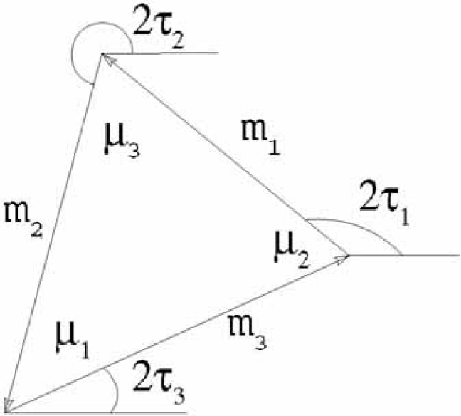
Figure 1: Vector triangle representing Eq. (27).

The problem reduces to one from elementary plane geometry. Given the three sides ($m_{i}$), of a triangle, find the three interior angles ($\mu_{i}$). We may start for example, by using the law of cosines to get

$$cos\mu_{1}=\frac{-m_{1}^{2}+m_{2}^{2}+m_{3}^{2}}{2m_{2}m_{3}},$$ (28)

and continue similarly to get the others. Finally the parameters $\tau_{i}$ which appear in the actual parameterization of Eq. (10) are found from Fig. 1 as

$$\tau_{1} = \frac{1}{6}(\pi-\mu_{1}-2\mu_{2}),$$

$$\tau_{2} = \frac{1}{6}(\pi+2\mu_{1}+\mu_{2}),$$

$$\tau_{3} = \frac{1}{6}(-2\pi-\mu_{1}+\mu_{2}).$$ (29)

In particular, the quantities

$$sin[2(\tau_{1}-\tau_{2})] = -sin(\mu_{1}+\mu_{2}),$$

$$sin[2(\tau_{1}-\tau_{3})] = sin\mu_{2},$$

$$sin[2(\tau_{2}-\tau_{3})] = -sin\mu_{1},$$ (30)

will turn out to be of interest. Actually, given the three interior angles $\mu_{i}$ of a triangle we do not get a unique choice of phase differences $(\tau_{i}-\tau_{j})$. While a rotation in the plane of the triangle will not change these phase differences, it is straightforward to see that the reflection of the triangle about any line in the plane will reverse the signs of all the phase differences. Thus there is another solution in which an extra minus sign appears on each right hand side of (30).

Now let us discuss the solutions of the complementary ansatz equation for various assumed values of $m_{3}$. In Table 1 the three real positive masses as well as the corresponding values of the two independent internal angles $\mu_{1},\mu_{2}$ of the triangle are listed. Of course, $\mu_{1}+\mu_{2}+\mu_{3}=\pi$. The solution with $B>0$ (type I with $m_{3}>m_{2}$) will be listed when it exists as well as the type II solution ($B<0$ or $m_{2}>m_{3}$).

Let us start with large values of $m_{3}$ and go down. Just from the ansatz there is no upper bound on the value of $m_{3}$. However there is a recent cosmology bound cosmobound which requires,

$$|m_{1}|+|m_{2}|+|m_{3}|<0.7\textrm{ eV}.$$ (31)

Thus values of $m_{3}$ greater than about 0.3 eV are physically disfavored. Table 1 shows that at this value both type I and type II solutions exist and correspond to almost equilateral triangles. This is true also for higher values of $m_{3}$. Notice that since the triangles are close to being equilateral, they have large interior angles and hence ( see for example Eq. (30)) large CP phases. The picture remains very similar down to around $m_{3}=0.1$ eV but as one gets closer to the value, roughly $0.0593$ eV, where the real type I solution of Eq. (18) exists, there is a marked change. It is seen that the interior angles of the type I solution become small as it prepares to go to the degenerate triangle corresponding to the real solution. We may get as small CP phases as we like by tuning close to the real solution; this is illustrated in Table 1 for a particular value of $m_{3}$. If one further lowers $m_{3}$, it is found that the type I solution no longer exists. On the other hand the type II solution persists and does not change much until $m_{3}$ approaches the small value of roughly 0.00068 eV. There are no solutions for $m_{3}$ smaller than this value. We can also tune $m_{3}$ as illustrated in the table to get as small CP phases as we like for the type II case. It should be remarked that the precise numbers in Table 1 are based on the assumption that the best fit numbers given in Eq. (1) are exact and hence are meaningful to the accuracy given only in the sense of comparing the various solutions with each other, not with experiment.

type	$m_{1},m_{2},m_{3}$ in eV	$\mu_{1},\mu_{2}$ in radians	$|m_{ee}|$ in eV	$\epsilon_{1}$, $\epsilon_{2}$, $\epsilon_{3}$
I	0.2955, 0.2956, 0.3000	1.038, 1.039	0.185	0.342, 0.433, 0.017
II	0.3042, 0.3043, 0.3000	1.055,1.056	0.187	0.330, 0.426, -0.0172
I	0.0856, 0.0860, 0.1000	0.946, 0.952	0.058	0.138, 0.060, 0.00137
II	0.1119, 0.1122, 0.1000	1.106, 1.111	0.065	0.194, 0.088-0.0024
I	0.0305, 0.0316, 0.0600	0.258, 0.268	0.030	0.00982, 0.00422, 0.00004
II	0.0783, 0.0787, 0.0600	1.172, 1.186	0.043	0.094, 0.041,-0.0011
I	0.0291, 0.0302, 0.0592715649	0.000552, 0.000574	0.030	1.96 $\times 10^{-6}$, 0.84 $\times 10^{-6}$, 0.71 $\times 10^{-7}$
II	0.0774, 0.0782, 0.0592715649	1.174, 1.188	0.042	0.047, 0.020, -0.0011
II	0.0643, 0.0648, 0.0400	1.243, 1.268	0.033	0.052, 0.023,-0.000681
II	0.0541, 0.0548, 0.0200	1.355. 1.417	0.024	0.018, 0.0078,-0.000335
II	0.0506, 0.0512, 0.0050	1.386, 1.658	0.021	0.0057, 0.0025,-0.0000824
II	0.0503, 0.0510, 0.0010	0.814, 2.313	0.021	0.00073, 0.00031,-0.0000122
II	0.0503, 0.0510, 0.0006811	0.051361, 3.089536	0.021	0.0000348, 0.0000150, -0.601 $\times 10^{-6}$

Table 1: Panorama of solutions as $m_{3}$ is lowered from about the highest value which is experimentally reasonable to the lowest value imposed by the model. In the type I solutions $m_{3}$ is the largest mass while in the type II solutions $m_{3}$ is the smallest mass. For each value of $m_{3}$, the values of the model predictions for $m_{1}$ and $m_{2}$ as well as the internal angles $\mu_{1}$ and $\mu_{2}$ are given. The model prediction for the neutrinoless double beta decay quantity $|m_{ee}|$ is next shown. Finally, the last column shows the estimated lepton asymmetries due to the decays of the heavy neutrinos. Note that the reversed sign of lepton asymmetry is also possible, as discussed in the text.

It is straightforward to give an analytic interpretation of the pattern of solutions just observed. First note that CP violation corresponds to a non degenerate triangle. Note also that the orientation of the triangle in the complex plane is just obtained by imposing the unimodularity condition for $\omega(\tau)$ in Eq. (10). Hence the internal angles, $\mu_{i}$ are really the intrinsic carriers of CP violation. The determinant of whether one has CP violation is the non vanishing of the quantity:

$${\cal A} = [m(m-m_{1})(m-m_{2})(m-m_{3})]^{1/2},$$

$$m = \frac{1}{2}(m_{1}+m_{2}+m_{3}),$$ (32)

which just expresses the area, ${\cal A}$ of a triangle in terms of the lengths of its sides. This area may be rewritten in the convenient form:

$${\cal A}=\frac{1}{4}\left([(m_{1}+m_{2})^{2}-m_{3}^{2}][m_{3}^{2}-(m_{1}-m_{2})^{2}]\right)^{1/2}.$$ (33)

Now we may see that the vanishing of the first factor corresponds to the type I real solution while the vanishing of the second factor corresponds to the type II real solution. Furthermore, for a solution to exist, the argument of the square root should be positive. With the second factor, that establishes the minimum allowed value of $m_{3}$ while with the first factor, that establishes the minimum value of $m_{3}$ which allows a type I solution.

An important test of the model is the experimental bound on neutrinoless double beta decay. This implies ndbdexpt

$$|m_{ee}|<(0.35\rightarrow 1.30)\textrm{ eV},$$ (34)

where

$$|m_{ee}|=|m_{1}(K_{exp11})^{2}e^{-2i\tau_{1}}+m_{2}(K_{exp12})^{2}e^{-2i\tau_{2}}+m_{3}(K_{exp13})^{2}e^{-2i\tau_{3}}|.$$ (35)

Using the parameterization of Eq. (9) and approximating $s_{13}=0$ (which is reasonable in the present model since $m_{3}$ is never much larger than $m_{1}$ or $m_{2}$), this can be written simply as:

$$|m_{ee}|=[(c_{12}^{2}m_{1})^{2}+(s_{12}^{2}m_{2})^{2}+2m_{1}m_{2}c_{12}^{2}s_{12}^{2}cos(\mu_{1}+\mu_{2})]^{1/2}.$$ (36)

Here Eqs. (29) were also used. Reading $s_{12}^{2}$ from (16) then enables us to calculate $|m_{ee}|$ for each line of Table I. It is seen that $|m_{ee}|$ decreases smoothly with decreasing $m_{3}$ for each of the type I and type II solutions. All the values of $m_{3}$ listed are consistent with the present bound. It is interesting that an improvement of the experimental bound by an order of magnitude Future would provide a good test of the model.

V Estimate for leptogenesis

When one adopts the SO(10) motivation for the present Ansatz, it turns out that the resulting model predicts in a simple way the properties of the heavy neutrinos which are intrinsically contained in the SO(10) theory. This feature may be used in connection with the leptogenesis mechanism leptogen of baryogenesis. According to this mechanism, the CP violating and lepton number violating decays of the heavy neutrinos at a high temperature (corresponding to the grand unification scale) in the very early universe establish a lepton asymmetry. As the universe cools further, the (B+L) violating but (B-L) conserving ”sphaleron” interaction sphaleron converts this into a baryon asymmetry which may be compared with the observed ratio of baryons to photons in the universe. There are many interesting discussions of this mechanism in the literature sakharov ; reviews ; lv ; lpyetal ; recent . Here, we will estimate the dependence on neutrino masses and CP phases of the predicted baryon asymmetry in the present model.

The starting point of this discussion is the Yukawa term of the Lagrangian density which describes the tree level decay of a heavy Majorana neutrino, $N_{j}$ (where the subscript denotes a 3-valued generation index) to a Higgs doublet member,

$$\Phi^{c}=\left(\begin{array}[]{c}{\bar{\phi}}^{0}\\ -\phi^{-}\end{array}\right)$$ (37)

plus the appropriate member of the left-handed lepton doublet,

$$L_{i}=\left(\begin{array}[]{c}\nu_{iL}\\ e_{iL}\end{array}\right).$$ (38)

Then the Yukawa term reads:

$${\cal L}_{Yukawa}=-\sum{\bar{L}}_{i}\lambda_{ij}\Phi^{c}N_{j}+H.c.,$$ (39)

where $\lambda_{ij}$ is the matrix of Yukawa coupling constants. We can simplify this expression, which is supposed to contain the fermion fields in prediagonal bases, in several ways. First, at the high temperature for which the N decays are relevant, the phase transition to spontaneously broken SU(2) x U(1) has not yet taken place. Thus we can consider the light fermions in $L_{i}$ to be massless and there is no need to insert suitable unitary matrices to bring the light field mass matrices to diagonal form. However the heavy neutrino, $N$ should be related to the physical field ${\hat{N}}$ with a unitary matrix $U$ as $N=U{\hat{N}}$. As mentioned in section I, if the SO(10) model contains only a single ”126” Higgs type field (although any number of “10”’s and “120”’s are allowed) and also if the first (non see-saw) term in Eq. (4) is dominant, the prediagonal mass matrices for the light and heavy neutrinos must be proportional to each other and the diagonalizing matrix $U$ must be the same one which appears in Eq. (13). Approximating, as we did earlier, $\Omega$ to be essentially the unit matrix we can set $U\approx K$. If the model of section IV is adopted, for example, we can specify $K$, including CP phases, to a fair approximation for each assumed value of $m_{3}$. Finally we approximate the matrix of Yukawa couplings by:

$$\lambda_{ij}\approx\frac{\delta_{ij}m_{i}^{U}}{r^{\prime}<\phi^{0}>},$$ (40)

where $m_{i}^{U}$ are the three charge 2/3 quark masses at a low energy scale, $r^{\prime}\approx 3$ is a suitable factor for running these masses from the grand unified scale to the low energy scale and $<\phi^{0}>\approx 246/{\sqrt{2}}$ GeV. Note that ${\cal L}_{Yukawa}$ is the term responsible for generating the neutrino Dirac matrix, $M_{D}$ in Eq. (4). In the simplest approximation to the SO(10) theory the charge 2/3 quark mass matrix and neutrino Dirac mass matrix are proportional to each other and diagonal (since the quark mixings are after all small).

Putting these things together we arrive at the “effective” term for calculating the heavy neutrino decays (at grand unified scale temperature):

$${\cal L}_{Yukawa}=-\sum{\bar{L}}_{i}h_{ij}\Phi^{c}{\hat{N}}_{j}+H.c.,$$ (41)

where

$$h_{ij}\approx\frac{m_{i}^{U}K_{expij}e^{-i\tau_{j}}}{<\phi^{0}>r^{\prime}}.$$ (42)

The quantities needed for the calculation are the matrix products $(h^{\dagger}h)_{ij}$. We may further simplify these products by noting that the top quark mass is much heavier than the others so the products approximately become $h_{i3}^{\dagger}h_{3j}$. Specifically, the diagonal products are:

$$(h^{\dagger}h)_{11} \approx (s_{12}s_{23}/r^{\prime})^{2},$$

$$(h^{\dagger}h)_{22} \approx (c_{12}s_{23}/r^{\prime})^{2},$$

$$(h^{\dagger}h)_{33} \approx (c_{12}/r^{\prime})^{2},$$ (43)

where we used the numerical coincidence that $m_{t}=<\phi>$. Furthermore, we set $s_{13}=0$ in agreement with the model of section IV ( See the parameterization of Eq. (9)). Numerically, with Eq. (16) and $(r^{\prime})^{2}\approx 10$ one obtains $(h^{\dagger}h)_{11}\approx 1.50\times 10^{-2}$, $(h^{\dagger}h)_{22}\approx 3.50\times 10^{-2}$ and $(h^{\dagger}h)_{33}\approx 7.00\times 10^{-2}$. In terms of these diagonal products, the tree level widths of the heavy neutrinos are given by,

$$\Gamma_{i}=\frac{(h^{\dagger}h)_{ii}M_{i}}{8\pi},$$ (44)

where $M_{i}$ is the mass of the ith heavy neutrino. The off diagonal products play an important role in determining the lepton asymmetry. They are explicitly given in the model of section IV as:

$$(h^{\dagger}h)_{12} \approx -s_{12}c_{12}s_{23}^{2}e^{i(\tau_{1}-\tau_{2})}/(r^{\prime})^{2},$$

$$(h^{\dagger}h)_{13} \approx s_{12}s_{23}c_{23}c_{13}e^{i(\tau_{1}-\tau_{3})}/(r^{\prime})^{2},$$

$$(h^{\dagger}h)_{23} \approx -s_{23}c_{12}c_{23}c_{13}e^{i(\tau_{2}-\tau_{3})}/(r^{\prime})^{2},$$

$$(h^{\dagger}h)_{ij} = (h^{\dagger}h)_{ji}^{\ast},$$ (45)

where the CP phases $\tau_{i}$ depend on the choice of $m_{3}$ as explained in section IV. Numerically, one has $(h^{\dagger}h)_{12}\approx-2.29\times 10^{-2}exp[i(\tau_{1}-\tau_{2})]$, $(h^{\dagger}h)_{13}\approx 2.74\times 10^{-2}exp[i(\tau_{1}-\tau_{3})]$ and $(h^{\dagger}h)_{23}\approx-4.18\times 10^{-2}exp[i(\tau_{2}-\tau_{3})]$. In arriving at these estimates from Eq. (16) we arbitrarily took all the signs of the trigonometric functions to be positive. This will not lead to any ambiguity since, for the application of interest, the off-diagonal products must be squared.

The lepton asymmetry $\epsilon_{i}$, due to the decay of the ith heavy neutrino is defined as the ratio of decay widths:

$$\epsilon_{i}=\frac{\Gamma(N_{i}\rightarrow L+\Phi)-\Gamma(N_{i}\rightarrow{\bar{L}}+{\bar{\Phi}})}{\Gamma(N_{i}\rightarrow L+\Phi)+\Gamma(N_{i}\rightarrow{\bar{L}}+{\bar{\Phi}})}.$$ (46)

In this formula $L+\Phi$ stands for all pairs of the types $e^{-}_{j}+\phi^{+}$ and $\nu_{j}+{\bar{\phi}}^{0}$. This is an effect which violates C and CP conservation, in agreement with the requirement of Sakharov sakharov . To get a non-zero value one must include the interference between the tree diagram from Eq.(41) and the one loop diagrams (of both “self-energy” and “triangle” types). If the masses of the heavy neutrinos are well separated the result leptogen ; pil is:

$$\epsilon_{i} = \frac{1}{8\pi}\sum_{j\neq i}\frac{Im[(h^{\dagger}h)_{ij}(h^{\dagger}h)_{ij}]}{(h^{\dagger}h)_{ii}}f(M_{j}^{2}/M_{i}^{2}),$$

$$f(x) = \sqrt{x}\left[\frac{1}{1-x}+1-(1+x)ln(1+1/x)\right].$$ (47)

Note that the contribution to the lepton asymmetry of the lightest heavy neutrino is expected to be the most important one for the final calculation of baryon asymmetry reviews .

Now let us make numerical estimates for the lepton asymmetries when all CP violation is due to Majorana phases (section IV). From Eq. (5) we relate the heavy neutrino masses to the light neutrino masses simply as:

$$M_{i}=cm_{i},$$ (48)

where $c$ is a real, positive constant. This equation has earlier been used jpr for the study of leptogenesis in the framework of a left-right symmetric model. It should be noted that renormalization group effects rge will modify the exact proportionality of the light and heavy neutrino masses as well as the equality of the corresponding diagonalizing matrices. This should be taken into account for a more accurate treatment. In the model of section IV the third neutrino is typically somewhat further away in mass from the other two, which are always relatively close. For example, in the type II situation, $m_{3}$ is the lightest of the light neutrino masses so $M_{3}$ will be the lightest of the heavy neutrino masses and the contribution to the lepton asymmetry is $\epsilon_{3}$. Using Eqs. (47), (48), (45) and (30) we obtain:

$$\epsilon_{3}\approx\left[-4.27f([m_{1}/m_{3}]^{2})sin\mu_{2}+9.94f([m_{2}/m_{3}]^{2})sin\mu_{1}\right]\times 10^{-4}.$$ (49)

Notice that $c$ has canceled out in this formula and also cancels out in the determination of the angles $\mu_{i}$. Thus the lepton asymmetry given by this formula does not depend on the overall scale of the heavy neutrino masses.

In the type I case, the heavy neutrino spectrum consists of two nearly degenerate lighter states, ($N_{1}$, $N_{2}$) and a heavier state, $N_{3}$. For the corresponding asymmetries $\epsilon_{1}$ and $\epsilon_{2}$, the diagrams involving self energy type corrections are enhanced since an internal heavy neutrino line will be close to its mass shell. The formulas pil thus, for greater accuracy, involve the decay widths and we will approximate:

$$\epsilon_{1} = \frac{Im[(h^{\dagger}h)_{12}(h^{\dagger}h)_{12}]}{(h^{\dagger}h)_{11}(h^{\dagger}h)_{22}}\frac{(M_{1}^{2}-M_{2}^{2})M_{1}\Gamma_{2}}{(M_{1}^{2}-M_{2}^{2})^{2}+M_{1}^{2}\Gamma_{2}^{2}},$$

$$\epsilon_{2} = \frac{Im[(h^{\dagger}h)_{12}(h^{\dagger}h)_{12}]}{(h^{\dagger}h)_{11}(h^{\dagger}h)_{22}}\frac{(M_{1}^{2}-M_{2}^{2})M_{2}\Gamma_{1}}{(M_{1}^{2}-M_{2}^{2})^{2}+M_{2}^{2}\Gamma_{1}^{2}}.$$ (50)

Again, we may replace the heavy neutrino masses using Eq. (48) and note that the factor $c$ cancels out. Inserting numbers, we obtain:

$$\epsilon_{1} \approx -\frac{1.39\times 10^{-3}sin(\mu_{1}+\mu_{2})m_{1}m_{2}(m_{1}^{2}-m_{2}^{2})}{(m_{1}^{2}-m_{2}^{2})^{2}+1.94\times 10^{-6}m_{1}^{2}m_{2}^{2}}$$

$$\epsilon_{2} \approx -\frac{5.96\times 10^{-4}sin(\mu_{1}+\mu_{2})m_{1}m_{2}(m_{1}^{2}-m_{2}^{2})}{(m_{1}^{2}-m_{2}^{2})^{2}+3.56\times 10^{-7}m_{1}^{2}m_{2}^{2}}.$$ (51)

The values of all these asymmetries for the range of possibilities are listed in the last column of table I.

Furthermore it must be noted that, owing to the non-uniqueness of sign for all of Eqs. (30), reversing the signs of all the lepton asymmetries also yields a solution corresponding to our initial Ansatz.

Although the scale of the heavy neutrinos has been seen to cancel out of the formulas (49) and (51) for the lepton asymmetries in favor of their ratios (which are the same as those of the light neutrinos in this model), there is nevertheless a consistency condition implied by the SO(10) motivation for the starting Ansatz. This arises since Eq. (39) is not only the source of the lepton asymmetry but also provides the seesaw contribution to the light neutrino masses. For our motivation we assumed that this contribution was dominated by the first term of Eq. (4). To make a rough estimate of what this means we assume all matrices of the seesaw term to be diagonal. Then the value of $c^{1/2}$ defined in Eq. (48) should be greater than $m_{i}^{U}/(m_{i}r^{\prime})$ in order that the first term of Eq. (4) be greater than the second term. In the case of the type I solution with $m_{3}\approx 0.06$ eV shown in Table I, this implies that the lightest heavy neutrino should be heavier than about 2.6 $\times 10^{13}$ GeV. For the case of the type II solution with $m_{3}\approx 7\times 10^{-4}$ eV, the lightest heavy neutrino should be heavier than about 4.4 $\times 10^{15}$ GeV.

The goal of the baryogenesis problem is to understand the ratio $\eta_{B}=n_{B}/n_{\gamma}$, the net baryon number density divided by the photon density. Experimentally, this quantity is foundcosmobound , from the study of big-bang nucleosynthesis, to be

$$\eta_{B}=(6.5\pm 0.4)\times 10^{-10}.$$ (52)

To obtain non-zero $\eta_{B}$, it is not sufficient, as pointed out by Sakharovsakharov , just to have non-zero values of the lepton asymmetry $\epsilon_{i}$, defined in Eq. (46). In addition, the CP violating decays of the heavy neutrinos must occur out of thermal equilibrium. A detailed treatment requires solution of the Boltzmann evolution equations for the system bdp . Here we shall make a rough estimate which we use to draw what might be a fairly robust conclusion.

First, we should remark that the baryon asymmetry generated by the sphaleron mechanism would be about -1/3 BL , (for a review see reviews ) of an initial lepton asymmetry. The lepton number violating decays of the ith heavy neutrino are usually roughly taken to be out of equilibrium if the decay rate $\Gamma_{i}$ in Eq. (44) is less than the Hubble rate,

$$H\approx 1.7g_{*}^{1/2}T^{2}/M_{P},$$ (53)

where $g_{*}\approx 100$ is the number of effective light degrees of freedom at the leptogenesis scale, $T$ is the temperature ( corresponding to the mass of the decaying heavy neutrino) and $M_{P}\approx 1.22\times 10^{19}$ GeV. In the present model this ratio takes the explicit form:

$$K_{i}=\frac{\Gamma_{i}}{H}\approx\frac{(h^{\dagger}h)_{ii}M_{P}}{427M_{i}},$$ (54)

which is seen to be inversely proportional to $M_{i}$. The net baryon asymmetry is estimated as reviews ,

$$\eta_{B}\approx-\frac{7}{3g_{*}}\sum\epsilon_{i}D_{i},$$ (55)

where the $D_{i}$ are suppression factors to be obtained by numerical solution bdp of the Boltzmann equations. It is generally accepted that only the contributions of the lightest heavy neutrinos should not get washed out; thus we will set $D_{i}$ =0 for the heavier neutrinos. If $10<K_{i}\lesssim 10^{6}$, the suppression factor is often approximated by the analytic form kt

$$D_{i}\approx\frac{0.3}{K_{i}[ln(K_{i})]^{0.6}}.$$ (56)

When $K_{i}<1$, the suppression factor is expected to be of order unity if $M_{i}$ is not too large. However, as $M_{i}$ gets larger there is a sizeable washout effect washout .

Glancing at the last column in table I and comparing with the experimental value of $\eta_{B}$ in Eq. (52) as well as Eqs. (55) and (56) suggests that the values of $\eta_{B}$ obtained for typical values of the assumed light neutrino mass parameter $m_{3}$ would be considerably larger than the experimental baryon asymmetry. However, we can expect to be able to obtain agreement with the experimental value since, as discussed in section IV, we may make the Majorana CP phases as small as we like by continuously tuning the independently chosen variable, $m_{3}$ so that the triangle of mass vectors gets arbitrarily close to one of the two degenerate straight line cases which causes ${\cal A}$ in Eq.(33) to vanish. Thus the solutions of the model which would be consistent with the observed baryon asymmetry correspond to neutrino masses more or less close the real cases of either Eq. (18) or Eq. (19).

The qualitative points: i. that in the present model the value of the free parameter, $m_{3}$ can always be tuned to be arbitrarily close to its values for the two real solutions (so that the CP violation and hence leptogenesis strength becomes as small as desired) and ii. that the characteristic lepton asymmetries, $\epsilon_{i}$ for values of $m_{3}$ away from these two real solutions are rather large, comprise the main result of our discussion of the application of the $Tr(M_{\nu})=0$ Ansatz to the baryogenesis problem. These points lead to the expectation that the physical value of $m_{3}$ is likely to be close to one of the two values in Eq. (18) or Eq. (19) and that this conclusion might persist even when our simplifications are not made. A more accurate treatment would include the features: a) effect of non-trivial charged lepton mixing matrix, b) renormalization group induced deviations from the “clone” treatment of the heavy Majorana neutrinos and c) full integration of the Boltzmann evolution equations. Even though our main conclusion is a qualitative one, it seems nevertheless an interesting exercise to find what values of light and heavy neutrino masses corrrespond to the correct order of magnitude of the observed baryon asymmetry. Note that the seeming great accuracy of the entries in Table I is not meant for precise comparison with experiment, but for comparison of the results of different $m_{3}$ choices with each other.

Specifically, consider the tuned type I solution in table I with $m_{3}\approx$ 0.05927 eV. We noted in the discussion after Eq. (51) that this would correspond to heavy neutrino “clone” masses $(M_{1},M_{2},M_{3})$ greater than about $(2.60,2.70,5.27)\times 10^{13}$ GeV, respectively. We assume that the two lighter neutrinos are the important ones and set $D_{3}$ = 0. The ratios $(K_{1},K_{2})$ defined in Eq. (54) would then be less than about (16.5, 37.1) and would result in suppression factors $(D_{1},D_{2})$ greater than (0.010, 0.0037). Using Eq. (55) and table I for $\epsilon_{1}$ and $\epsilon_{2}$ then gives $|\eta_{B}|$ = 5.4 $\times 10^{-10}$, close to the experimental value in Eq.(52). This can be adjusted by further tuning $m_{3}$ or to some extent by varying the overall mass scale of $(M_{1},M_{2},M_{3})$.

For the type II case, first consider the solution in table I with $m_{3}\approx$ 0.0007 eV. As discussed before, this would correspond to heavy neutrino “clone” masses $(M_{1},M_{2},M_{3})$ greater than about (320, 320, 4.4) $\times 10^{15}$ GeV. In this case, $M_{3}$ is the lightest of the three heavy neutrinos and is assumed to be the relevant one. We thus set $D_{1}=D_{2}=0$. The ratio $K_{3}$ given in Eq. (54) is then about 0.45 and indicates that the lightest heavy neutrino is, as desired, decaying out of equilibium. However, because its mass is considerably higher than that of the type I case just discussed, there is more wash out washout , $D_{3}\approx 3.5\times 10^{-5}$. Reading $\epsilon_{3}$ from table I then gives $\eta_{B}\approx 5\times 10^{-13}$, about three orders of magnitude too small. Thus we must raise the value of $m_{3}$ a bit. Backing off a little to the case $m_{3}\approx$ 0.005 eV in table I increases the value of $\epsilon_{3}$ and also allows us (in line with the dominance of the first term in Eq.(4)) to choose the lower bound of $M_{3}$ to be smaller, around 6 $\times 10^{14}$ GeV. This results in an estimate $|\eta_{B}|\approx 16\times 10^{-10}$, which is the correct order of magnitude. One might wonder whether the contributions to $\eta_{B}$ from $\epsilon_{1}$ and $\epsilon_{2}$ are completely washed out in a case like the present. However, even if they were dominant, it would just require us to tune more closely toward small $m_{3}$.

Thus, if the model of CP violation with just the Majorana phases is correct, the magnitude of the baryon to photon ratio can be understood when either the sum of the three light neutrino masses is about 0.118 eV and $|m_{ee}|$ =0.030 eV (type I) or the sum of the three light neutrino masses is about 0.107 eV and $|m_{ee}|$= 0.021 eV (type II). In both cases the CP violating Majorana phases are extremely small. That might suggest a possible model in which a small CP violating perturbation due to some separate effect modifies an otherwise CP conserving lepton sector.

We can also calculate the baryon to photon ratio in the model of section III, where $\delta$ is the only CP violating phase. There we noted that the only possible choices of $\delta$ consistent with our Ansatz satisfy $sin^{2}\delta=1$. Then we have the type I solution for light neutrino masses given in Eq. (25) and the type II solution given in Eq. (26). The corresponding CP violation factors are now (to first order in the small parameter $s_{13}$) for the type I case:

$$Im[(h^{\dagger}h)_{12}(h^{\dagger}h)_{12}] \approx \frac{s_{13}sin\delta sin(2\theta_{12})}{(r^{\prime})^{4}}c_{23}s_{23}^{3},$$

$$Im[(h^{\dagger}h)_{13}(h^{\dagger}h)_{13}] \approx -\frac{s_{13}sin\delta sin(2\theta_{12})}{(r^{\prime})^{4}}s_{23}c_{23}^{3},$$

$$Im[(h^{\dagger}h)_{23}(h^{\dagger}h)_{23}] \approx -Im[(h^{\dagger}h)_{13}(h^{\dagger}h)_{13}],$$ (57)

and for the type II case:

$$Im[(h^{\dagger}h)_{12}(h^{\dagger}h)_{12}] \approx -\frac{s_{13}sin\delta sin(2\theta_{12})}{(r^{\prime})^{4}}c_{23}s_{23}^{3},$$

$$Im[(h^{\dagger}h)_{13}(h^{\dagger}h)_{13}] \approx \frac{s_{13}sin\delta sin(2\theta_{12})}{(r^{\prime})^{4}}s_{23}c_{23}^{3},$$

$$Im[(h^{\dagger}h)_{23}(h^{\dagger}h)_{23}] \approx Im[(h^{\dagger}h)_{13}(h^{\dagger}h)_{13}],$$ (58)

As in the cases where only the Majorana phases contribute to the CP violation, the predicted lepton asymmetries, $\epsilon_{i}$ will typically lead to a value of the baryon to photon ratio much larger than the experimental one. In the present case it is not possible to fine tune $\delta$. The only possibility would be to fine tune $s_{13}$ to an extremely small value. This seems more artificial since $s_{13}$ is not required to vanish in the CP conserving situation. In any event, an experimental measurement of non-zero $s_{13}$ would, practically speaking, rule out this case as a candidate for leptogenesis.

VI Discussion and summary

In this paper, we investigated an Ansatz which correlates information about the four quantities in the light neutrino sector which are not yet known from experiment; namely, the absolute mass of any particular neutrino, the “conventional” CP violation phase and the two Majorana phases. Of course, with input from analyses of neutrino oscillation experiments, the masses of the other two neutrinos can be found, up to a discrete ambiguity, if the mass of one is specified. The results of the present paper can be used for calculating many quantities of experimental interest like the neutrinoless double beta decay amplitude factor $m_{ee}$ (presented in section IV) and various lepton number violating decays.

The Ansatz is not completely predictive, unless some assumptions are made. We first reviewed the case of assumed CP conservation (where just the three neutrino masses are obtained).Then we showed that if only the “conventional” CP violation phase is assumed to be non-zero, its value is fixed by the Ansatz to be maximal. A possibly more interesting case appears if we assume that only the two Majorana phases are non-zero. This enables us to scan the limited allowed range of assumed neutrino mass, $m_{3}$ (say) and find the other two neutrino masses as well as the two Majorana phases for each value of $m_{3}$. The result seems to cut through a “cross section” of interesting possibilities which are described in a simple way. The still more complicated case without setting any of the three CP phases to zero gives a two parameter family of solutions and will be treated elsewhere. Another (common) assumption we made for a first analysis is that the measured lepton mixing matrix is dominated by the neutrino factor. This is consistent with the finding in recent years that the mixing in the neutrino sector is apparently much larger than the mixing in the quark sector (which in models is usually relatively small and similar to that of the charged lepton factor).

It seems relevant to discuss briefly the status of the motivations for the complementary Ansatz we are using. One motivation, based on a loop mechanism for generating neutrino masses was discussed recently by He and Zee hz . Our motivation bfns was based on the grand unification group SO(10). This group is well known to have the elegant feature that it accomodates one generation of elementary fermions as well as an extra (now desired) neutrino field in its fundamental spinor irreducible representation. Naturally, there are many possibilities for doing a detailed calculation using this group. One may ask whether it should be regarded as being derived from a superstring theory, whether it should be supersymmetric, whether the symmetry breakdown should be dynamical, whether the symmetry breakdown should be induced by Higgs fields and if so what kind and how many, etc? We focus, in our motivation, on the conventional possibility of using Higgs fields since it seems almost kinematical now (although since no Higgs field has yet been seen one should keep an open mind). Of course, there have been many interesting treatments along these lines so10studies . Our Ansatz is suggested by a relation involving only the neutrino mass matrix which might be true (or at least approximately correct) in a large number of models. In SO(10), tree level masses from a renormalizable Lagrangian can be obtained by using any number of Higgs mesons belonging to the 10, 120 and 126 dimensional representations. However, examining the form of the predicted mass matrices shows that the following fairly general relation jrs holds:

$$Tr(M^{D}-rM^{E})\propto Tr(M_{L}),$$ (59)

for any number of 10’s and 120’s but only a single 126 present. Here $M^{D}$ and $M^{E}$ are respectively the prediagonal mass matrices of the charge -1/3 quarks and charge -1 leptons while $r\approx 3$, as previously mentioned. $M_{L}$, which arises from the 126 Higgs field Yukawa couplings, is the non seesaw part of the light neutrino mass matrix which appears in Eq. (4). Taking traces cancels the contributions (antisymmetric matrices) of any 120 Higgs multiplets to the left hand side. Then, assuming the transformations which bring $M^{D}$ and $M^{E}$ to diagonal form to be roughly close to the identity we observe that the left hand side is approximately equal to $m_{b}-rm_{\tau}$, which is about zero. In fact this is a characteristic prediction of grand unification. In turn the right hand side gives us the starting Ansatz when it is assumed that the non seesaw term dominates in Eq. (4). Of course, if this domination is to hold the masses of the heavy neutrinos should not be too low. The present paper is in effect exploring the range of possibilities which exist when these assumptions are made in SO(10) models. An interesting question is whether this kind of limit or the pure seesaw limit gives a better description of nature, even if both terms are actually required.

We remark that SO(10) also gives another similar relation,

$$Tr(M^{U}-r^{\prime}M_{D})\propto Tr(M_{L}),$$ (60)

when only one 126 Higgs field exists. Here $M^{U}$ and $M_{D}$ respectively denote the prediagonal charge 2/3 quark mass matrix and the prediagonal neutrino “Dirac” matrix connecting the heavy and light neutrino fields.

An intriguing way to learn more about CP violation in the lepton sector is the study of the leptogenesis mechanism of baryogenesis. We saw that the treatment of this process simplifies when one adopts the present SO(10) motivation. Then the light neutrino mass matrix $M_{\nu}$ and $M_{L}$ are approximately equal and proportional (due to the assumption of only one 126 field in the theory) to the heavy neutrino mass matrix $M_{H}$. The only free parameter for the heavy neutrinos is their overall mass scale and this should not be too small to preserve non seesaw dominance. We showed in section V that it is easy to estimate the lepton asymmetry parameters $\epsilon_{i}$ for a “panorama” of values of the independent variable $m_{3}$ since they are actually independent of the overall heavy neutrino mass scale. As far as the resulting baryon to photon ratio, $\eta_{B}$ (parameterized in Eq. (55)) is concerned, the typical values of the $\epsilon_{i}$ give $\eta_{B}$ much greater than the experimental one for suppression factors $D_{i}$ of order unity. We observed that if the suppression factors are not too small one can therefore always choose a value of $m_{3}$ close enough to one of the two essentially different CP conserving solutions so that the Majorana phases are small enough to get experimental agreement for $\eta_{B}$. Using estimates of the suppression factors taken from other earlier studies, we noted that this conclusion seems reasonable. Of course the study of the suppression factors by solving the Boltzmann evolution equations is an important topic which involves many subtleties and would repay further work in the present model. Finally, the posible indication of very small CP phases might suggest a model in which the CP violation in the lepton sector has a separate identifiable source.

References

- (1) KamLAND collaboration, K. Eguchi et al, Phys. Rev. Lett. 90, 021802 (2003).
- (2) SNO collaboration, Q. R. Ahmad et al, arXiv:nucl-ex/ 0309004.
- (3) K2K collaboration, M. H. Ahn et al, Phys. Rev. Lett. 90, 041801 (2003).
- (4) For recent reviews see, for examples, S. Pakvasa and J. W. F. Valle, arXiv:hep-ph/0301061 and V. Barger, D. Marfatia and K. Whisnant, arXiv:hep-ph/0308123.
- (5) LSND collaboration, C. Athanassopoulos et al, Phys. Rev. Lett. 81, 1774 (1998).
- (6) M. Maltoni, T. Schwetz, M. A. Tortola and J. W. F. Valle, arXiv:hep-ph/0309130.
- (7) D. Black, A. H. Fariborz, S. Nasri and J. Schechter, Phys. Rev. D62, 073015 (2000).
- (8) H. Georgi, Particles and Fields (1974), edited by C. E. Carlson (AIP, New York, 1975), p. 575; H. Fritzsch and P. Minkowski, Ann. Phys. (NY) 93, 193 (1975); Nucl. Phys. B103, 61 (1976).
- (9) X.-G. He and A. Zee, Phys. Rev. D68, 037302, (2003).
- (10) M. Chanowitz, J. Ellis and M. K. Gaillard, Nucl. Phys. B128, 506 1977; A. J. Buras, J. Ellis, M. K. Gaillard and D. V. Nanopoulos, ibid B135, 66 1978.
- (11) T. Yanagida. in Proceedings of the workshop on unified theory and baryon number in the universe, edited by O. Sawada and A. Sugamoto, KEK report 79-18, Tsukuba, 1979, p. 95; M. Gell-Mann, P. Ramond and R. Slansky, in Supergravity, edited by P. van Niewenhuizen and D. Z. Freedmann (North-Holland, Amsterdam,1979); R. N. Mohapatra and G. Senjanovic, Phys. Rev. Lett. 44, 912 (1980).
- (12) T. Ohlsson and H. Snellman, Phys. Rev. D60, 093007 (1999). See also R. P. Thun and S. Mckee, Phys. Lett. B439, 123 (1998); G. Barenboim and F. Scheck, ibid B440, 332 (1998); G. Conforto, M. Barrone and G. Grimani, ibid, B447, 122 (1999); I. Stancu, Mod. Phys. Lett. A14, 689 (1999); A. Acker and S. Pakvasa, Phys. Lett. B397, 209 (1997). Criticism of this approach has been expressed by G. L. Fogli, E. Lisi, A. Marrone and G. Scioscia, hep-ph/9906450.
- (13) W. Rodejohann, Phys. Lett. B579, 127 (2004).
- (14) M. Fukugita and T. Yanagida, Phys. Lett. B174, 45 (1986).
- (15) J. Schechter and J. W. F. Valle, Phys. Rev. D 22, 2227 (1980).
- (16) S. M. Bilenky, J. Hosek and S. T. Petcov, Phys. Lett. 94B, 495 (1980).
- (17) M. Doi, T. Kotani, H. Nishiura, K. Okuda and E. Takasugi, Phys. Lett. 102B, 323 (1981).
- (18) J. Schechter and J. W. F. Valle, Phys. Rev. D23, 1666 (1981); A. de Gouvea, B. Kayser and R. N. Mohapatra, Phys. Rev. D67, 053004 (2002).
- (19) A. de Gouvea, A. Friedland and H. Murayama, Phys. Lett. B490, 125 (2000).
- (20) See the discussion in section IV of bfns above and L. Wolfenstein, Phys. Lett. 107B, 77 (1981).
- (21) D. N. Spergel et al, arXiv:astro-ph/0302209; S. Hannestad, arXiv:astro-ph/0303076.
- (22) H. V. Klapdor-Kleingrothaus et al, Eur. Phys. J. A12 147 (2001).
- (23) G. Gratta, Talk given at XXI International Syposium on Lepton and Photon Interactions at High Energies, 11-16 August 2003, Fermi National Accelerator Laboratory, Batavia, Illinois USA, IJMPA 19 A8,1115 (2004).
- (24) V. A. Kuzmin, V. A. Rubakov and M. E. Shaposhnikov, Phys. Lett. B155, 36(1985).
- (25) The original mechanism is given in A. D. Sakharov, Pis’ma Zh. Eksp. Teor. Fiz. 5, 24 (1967) (JETP Lett. 5, 24 (1967)).
- (26) J. A. Harvey and M. Turner, Phys. Rev. D42, 3344 (1990).
- (27) Reviews are given in E. W. Kolb and M. S. Turner, The Early Universe, (Addison-Wesley, Reading, MA, 1989); A. Pilaftsis, Int. J. Mod. Phys. A14, 1811 (1999) ; A. Riotto and M. Trodden, Annu. Rev. Nucl. Part. Sci. 45, 35 (1999).
- (28) M. A. Luty, Phys. Rev. D45, 455 (1992); C. E. Vayonakis, Phys. Lett. B286, 92 (1992).
- (29) P. Langacker, R. D. Peccei and T. Yanagida, Mod. Phys. Lett. A1, 541 (1986); R. N. Mohapatra and X. Zhang, Phys. Rev. D45, 5331 (1992); K. Enqvist and I. Vilja, Phys. Lett. B299, 281 (1993); H. Murayama, H. Suzuki, T. Yanagida and J. Yokoyama Phys. Rev. Lett. 70, 1912 (1993); T. Gherghetta and G. Jungman, Phys. Rev. D48, 1546 (1993), A. Acker, H. Kikuchi, E. Ma and U. Sarkar, Phys. Rev. D48, 5006 (1993); P. J. O’ Donnell and U. Sarkar, Phys. Rev. D49, 2118 (1994); M. P. Worah, Phys. Rev. D53, 3902 (1996); R. Jeannerot, Phys. Rev. Lett. 77, 3292 (1996); L. Covi, E. Roulet and F. Vissani, Phys. Lett. B384, 169 (1996); W. Buchmuller and M. Plumacher, Phys. Lett. B389, 73 (1996); G. Lazarides, Q. Shafi and N. D. Vlachos, Phys. Lett. B427, 53 (1998); J. Liu and G. Segre, Phys. Rev. D48, 4609 (1993); M. Flanz, E. A. Paschos, U. Sarkar and J. Weiss, Phys. Lett. B389, 693 (1996).
- (30) Recent discussions include:M. S. Berger and B. Brahmachari, Phys. Rev. D60, 073009 (2000); D. Falcone and F. Tramantano, Phys. Rev. D63, 073007 (2001); F. Bucella, Phys. Lett. B524, 241 (2002); H. B. Nielsen and Y. Takanishi, Phys. Lett. B507, 241 (2001); M. Hirsch and S. F. King, Phys. Rev. D64, 113005 (2001); Z. Z. Xing, Phys. Lett. B545, 352 (2002); P. H. Frampton, S. L. Glashow and T. Yanagida, Phys. Lett. B548, 119 (2002); T. Endoh et al, Phys. Rev. Lett. 89, 231601 (2002); S. Davidson and A. Ibarra, Nucl. Phys. B648, 345 (2003); G. C. Branco et al arXiv:hep-ph/0211001; J. Pati, Phys. Rev. D68, 072002 (2003); J. Ellis and M. Raidal, arXiv:hep-ph0206174; W. Buchmuller, P. Di Bari and M. Plumacher, arXiv:/0205349; S. Pascoli, S. T. Petcov and W. Rodejohann; arXiv:hep-ph/0302054; E. Kh. Akhmedov, M. Frigerio and A. Yu. Smirnov, arXiv:/hep-ph0305322; V. Barger, D. A. Dicus, H-J. He and T. Li, Phys. Lett. B583, 173 (2004).
- (31) See A. Pilaftsis in reviews above.
- (32) A. S. Joshipura, E. A. Paschos and W. Rodejohann, J. H. E. P. 0108, 029 (2001); W. Rodejohann, Phys. Lett. B452, 100 (2002).
- (33) See for examples, J. A. Casas et al, Nucl. Phys. B573, 652 (2000) and S. Autusch et al, Nucl. Phys. B674, 401 (2003).
- (34) A recent discussion is given by W. Buchmuller, P. Di Bari and M. Plumacher in recent above.
- (35) See Kolb and Turner in reviews above.
- (36) We use Fig 5a in bdp to roughly estimate the when necessary. Note that the horizontal axis is interpreted as roughly and the vertical axis as roughly .
- (37) K. Matsuda, Y. Koide, T. Fukuyama and H. Nishiura, Phys. Rev. D65, 033008 (2002), E 079904; B. Bajc, G. Senjanovic and F. Vissani, Phys. Rev. Lett. 90, 051802 (2003); K. Babu and C. Macesanu, private communication.
- (38) R. Johnson, S. Ranfone and J. Schechter, Phys. Rev. 35, 282 (1987). Here, =0 was studied in an SO(10) model together with the assumption of a special form for all the mass matrices. The more recent discovery of a top quark mass greater than about 90 GeV has ruled out that special form which, combined with =0, would make a singular matrix; H. S. Goh, R. N. Mohapatra and S. P. Ng; Phys. Lett B570, 215 (2003).